GOLDRUSH. IV. Luminosity Functions and Clustering Revealed with $\sim$4,000,000 Galaxies at $z\sim 2-7$: Galaxy-AGN Transition, Star Formation Efficiency, and Implication for Evolution at $z>10$

Abstract

We present new measurements of rest-UV luminosity functions and angular correlation functions from 4,100,221 galaxies at $z\sim 2-7$ identified in the Subaru/Hyper Suprime-Cam survey and CFHT Large-Area $U$-band Survey. The obtained luminosity functions at $z\sim 4-7$ cover a very wide UV luminosity range of $\sim 0.002-2000L_{\mathrm{UV}}^{*}$ combined with previous studies, confirming that the dropout luminosity function is a superposition of the AGN luminosity function dominant at $M_{\mathrm{UV}}\lesssim-24\,\mathrm{mag}$ and the galaxy luminosity function dominant at $M_{\mathrm{UV}}\gtrsim-22\,\mathrm{mag}$, consistent with galaxy fractions based on 1037 spectroscopically-identified sources. Galaxy luminosity functions estimated from the spectroscopic galaxy fractions show the bright end excess beyond the Schechter function at $\gtrsim 2\sigma$ levels, possibly made by inefficient mass quenching, low dust obscuration, and/or hidden AGN activity. By analyzing the correlation functions at $z\sim 2-6$ with halo occupation distribution models, we find a weak redshift evolution (within $0.3\,\mathrm{dex}$) of the ratio of the star formation rate (SFR) to the dark matter accretion rate, $SFR/\dot{M}_{\mathrm{h}}$, indicating the almost constant star formation efficiency at $z\sim 2-6$, as suggested by our earlier work at $z\sim 4-7$. Meanwhile, the ratio gradually increases with decreasing redshift at $z<5$ within $0.3\,\mathrm{dex}$, which quantitatively reproduces the cosmic SFR density evolution, suggesting that the redshift evolution is primarily driven by the increase of the halo number density due to the structure formation, and the decrease of the accretion rate due to the cosmic expansion. Extrapolating this calculation to higher redshifts assuming the constant efficiency suggests a rapid decrease of the SFR density at $z>10$ with $\propto 10^{-0.5(1+z)}$, which will be directly tested with JWST.

1. Introduction

Studying statistical properties of galaxies is important to understand the overall picture of galaxy formation and evolution. To quantify galaxy build-up in the early universe, many studies have investigated luminosity functions (i.e., one-point statistics) and angular correlation functions (i.e., two-point statistics) of high redshift galaxies. The luminosity function represents the volume density of galaxies as a function of the luminosity. Since galaxies form in dark matter halos, the luminosity function is related to the dark matter mass function and baryonic physics of galaxy formation. Studying the shape and evolution of the luminosity function in the high redshift universe allows us to obtain key insights into the star formation and feedback processes.

Great progress has been made in determining luminosity functions of high redshift galaxies, especially in the rest-frame ultraviolet (UV), which is redshifted to the optical wavelength at $z\sim 4-7$ easily accessible from ground-based telescopes. Since the time-averaged unobscured star formation rate (SFR) of galaxies is proportional to the luminosity of galaxies in the rest-frame UV, the UV luminosity function provides us with a measure of how quickly galaxies grow with cosmic time. Analyses of galaxies in deep blank fields including the Hubble Ultra Deep field (HUDF) have resulted in identifying $\sim 20,000$ galaxy candidates at $z\sim 2-10$ down to the absolute UV magnitude of $M_{\mathrm{UV}}\sim-17$ mag (e.g., Oesch et al. 2010, Ellis et al. 2013; Schenker et al. 2013; McLure et al. 2013; Bouwens et al. 2015, 2019, 2021; Finkelstein et al. 2015b; Parsa et al. 2016; Mehta et al. 2017). In addition, the gravitational lensing by galaxy clusters has allowed us to probe even fainter galaxies and constrain the faint-end slope of the UV luminosity function (e.g., Ishigaki et al. 2015, 2018; Oesch et al. 2015, 2018, Atek et al. 2015, 2018; Castellano et al. 2016; Alavi et al. 2016; McLeod et al. 2016, Bouwens et al. 2017), although the impact of magnification uncertainties should be correctly considered (see Bouwens et al. 2017, Atek et al. 2018).

Investigating the bright-end of the luminosity function is also important. Previously the luminosity function is thought to follow the Schechter function (Schechter 1976), which is derived from the shape of the halo mass function (Press & Schechter 1974) with several modifications. The Schechter function has an exponential cutoff at the bright end, which is possibly attributed to several different mechanisms such as heating from an active galactic nucleus (AGN; e.g., Binney 2004; Scannapieco & Oh 2004; Granato et al. 2004; Croton et al. 2006; Bower et al. 2006), inefficiency of gas cooling in massive dark matter haloes due to virial shock heating (e.g., Binney 1977; Rees & Ostriker 1977; Silk 1977; Benson et al. 2003), and dust obscuration which becomes substantial for the most luminous galaxies (e.g., Wang & Heckman 1996; Adelberger & Steidel 2000; Martin et al. 2005, Bowler et al. 2020). However, recent studies based on wide area surveys have reported an overabundance of objects at the bright end of UV luminosity functions beyond the Schechter function (bright end excess, e.g., Bowler et al. 2014, 2015, 2017, 2020; Stefanon et al. 2017, 2019; Ono et al. 2018; Stevans et al. 2018; Morishita et al. 2018; Adams et al. 2020; Moutard et al. 2020; Finkelstein et al. 2021). These studies suggest that the bright-end ($\leq-23$ mag) of the luminosity function is contributed by faint quasars or AGNs, at least at $z\sim 4-7$ (Ono et al. 2018; Stevans et al. 2018; Adams et al. 2020). In addition, Ono et al. (2018) calculate the galaxy UV luminosity function that is estimated by the subtraction of the AGN contribution, and report that the galaxy luminosity function still shows a bright end excess beyond the Schechter function at $z\sim 4-7$. They claim that this bright end excess implies inefficient mass quenching (e.g., the AGN feedback, virial shock heating) in these high redshift galaxies, or significant number of merging or gravitationally-lensed galaxies at the bright end (see also; e.g., Bowler et al. 2014; Bouwens et al. 2015).

Together with studying luminosity functions, the clustering analysis with the angular correlation function is important to understand the connection between galaxies and their dark matter halos. The galaxy-dark matter halo connection is investigated with the weak lensing analysis (e.g., Leauthaud et al. 2012; More et al. 2015; Coupon et al. 2015), the abundance matching/empirical model (e.g., Behroozi et al. 2013, 2019; Moster et al. 2013, 2018; Finkelstein et al. 2015a), and the clustering analysis (e.g., Harikane et al. 2016, 2018a; Ishikawa et al. 2017, 2020; Cowley et al. 2018; Qiu et al. 2018; Cheema et al. 2020). Since the weak lensing analysis cannot be applied at $z\gtrsim 2$ due to the limited number of the background galaxies and their lower image quality with current observational datasets (but see also Miyatake et al. 2021), the clustering analysis is a crucial tool for estimating the dark matter halo mass of high redshift galaxies. Many studies have investigated the dark matter halos of high redshift galaxies as a function of their redshifts and UV luminosities (e.g., Ouchi et al. 2004, 2005; Hildebrandt et al. 2009; Savoy et al. 2011; Bian et al. 2013; Barone-Nugent et al. 2014; Harikane et al. 2016, 2018b; Hatfield et al. 2018). These studies reveal that the more UV luminous galaxies reside in more massive halos.

Recently, Harikane et al. (2018b) have identified a tight relation between the ratio of the SFR to the dark matter accretion rate, $SFR/\dot{M}_{\mathrm{h}}$, and the halo mass, $M_{\mathrm{h}}$, over $z\sim 4-7$, suggesting the existence of a fundamental relation between the galaxy growth and its dark matter halo assembly. This redshift-independent relation indicates that the star formation efficiency does not significantly change at $z\sim 4-7$, and star formation activities are regulated by the dark matter mass assembly. Several studies show that this redshift-independent $SFR/\dot{M}_{\mathrm{h}}-M_{\mathrm{h}}$ relation can reproduce the UV luminosity functions at $z\gtrsim 4$ (e.g., Mason et al. 2015a; Harikane et al. 2018a; Tacchella et al. 2018; Bouwens et al. 2021) and the trend of the redshift evolution of the cosmic SFR density (e.g., Mason et al. 2015a; Harikane et al. 2018a; Tacchella et al. 2018; Oesch et al. 2018), a.k.a the cosmic star formation history or the Lilly-Madau plot (e.g., Lilly et al. 1996; Madau et al. 1996; Sawicki et al. 1997; Steidel et al. 1999; Bouwens et al. 2015; see review by Madau & Dickinson 2014). As discussed in Harikane et al. (2018a), this suggests a simple picture that the evolution of the cosmic SFR density is primarily driven by the steep increase of the number density of halos (and galaxies) due to the structure formation to $z\sim 4-2$, and the decrease of the accretion rate from $z\sim 2$ to $z\sim 0$ due to the cosmic expansion. However, the $SFR/\dot{M}_{\mathrm{h}}-M_{\mathrm{h}}$ relation is only constrained at $z\sim 4-7$, and it is not known whether the relation evolves from $z\sim 4$ to $z\sim 1-3$ or not, where the cosmic SFR density reaches its peak.

Table 1HSC-SSP Data Used for the $z\sim 4-7$ Selection

Field	R.A.	Decl.	Area	$g$	$r$	$i$	$z$	$y$
(1)	(2)	(3)	(4)	(5)	(6)	(7)	(8)	(9)
UltraDeep (UD)
UD-SXDS	02:18:23.26	$-$04:52:51.40	1.3	27.15	26.68	26.57	26.09	25.27
UD-COSMOS	10:00:23.43	$+$02:12:39.11	1.3	26.85	26.58	26.75	26.56	25.90
Deep (D)
D-XMM-LSS	02:25:26.62	$-$04:20:10.79	2.2	26.83	26.18	25.87	25.73	24.47
D-COSMOS	10:00:33.67	$+$02:10:07.02	4.9	26.61	26.37	26.32	26.02	25.15
D-ELAIS-N1	16:10:56.49	$+$54:58:13.69	5.4	26.71	26.34	26.13	25.73	24.81
D-DEEP2-3	23:28:17.72	$-$00:15:57.55	5.1	26.78	26.38	25.98	25.73	24.98
Wide (W)
W-W02	02:15:36.65	$-$04:03:28.04	33.3	26.43	25.94	25.69	25.03	24.22
W-W03	09:23:02.23	$+$00:36:45.81	66.2	26.20	25.84	25.76	25.17	24.36
W-W04	13:21:04.83	$-$00:12:07.68	72.2	26.41	25.99	25.86	25.17	24.33
W-W05	21:26:59.14	$+$01:41:02.30	86.6	26.18	25.81	25.61	25.01	24.25
W-W06	15:38:28.05	$+$43:18:51.64	28.4	26.44	26.05	25.78	25.09	24.15
W-W07	14:17:03.01	$+$52:30:29.70	0.9	26.60	25.88	25.79	24.98	24.00
Total Area			307.9

Note. — (1) Field name. (2) Right ascension. (3) Declination. (4) Effective area in $\mathrm{deg^{2}}$. (5)-(9) $5\sigma$ limiting magnitude measured in $1.$​​″$5$ diameter circular apertures in the $g$-, $r$-, $i$-, $z$-, and $y$-bands. These limiting magnitudes are not corrected to total.

In this work, we present new measurements of the rest-frame UV luminosity functions at $z\sim 4-7$ and clustering at $z\sim 2-6$ based on wide and deep optical images obtained in the Hyper-Suprime Cam Subaru Strategic Program (HSC-SSP) survey (Aihara et al. 2018, see also Miyazaki et al. 2012, 2018; Komiyama et al. 2018; Furusawa et al. 2018) and the CFHT large area U-band deep survey (CLAUDS; Sawicki et al. 2019). This paper is one in a series of papers from twin programs dedicated to scientific results on high redshift galaxies based on the HSC-SSP survey data. One program is our luminous Lyman break galaxy (LBG) or dropout galaxy studies, named Great Optically Luminous Dropout Research Using Subaru HSC (GOLDRUSH; Ono et al. 2018, Harikane et al. 2018a, Toshikawa et al. 2018). The other program is high redshift Ly$\alpha$ emitter (LAE) studies using HSC narrowband filters, Systematic Identification of LAEs for Visible Exploration and Reionization Research Using Subaru HSC (SILVERRUSH; Ouchi et al. 2018; Shibuya et al. 2018a, b; Konno et al. 2018; Harikane et al. 2018b, 2019; Inoue et al. 2018; Higuchi et al. 2019; Kakuma et al. 2019; Ono et al. 2021). Our new LBG catalogs are made public on our project webpage or zenodo.

This paper is organized as follows. We show the observational datasets in Section 2 and describe sample selections in Section 3. The results of the UV luminosity functions and clustering analysis are presented in Sections 4 and 5, respectively. We discuss our results in Section 6, and summarize our findings in Section 7. Throughout this paper we use the Planck cosmological parameter sets of the TT, TE, EE+lowP+lensing+ext result (Planck Collaboration et al. 2016): $\Omega_{\mathrm{m}}=0.3089$, $\Omega_{\Lambda}=0.6911$, $\Omega_{\mathrm{b}}=0.049$, $h=0.6774$, and $\sigma_{8}=0.8159$. We define $r_{\mathrm{200}}$ that is the radius in which the mean enclosed density is 200 times higher than the mean cosmic density. To define the halo mass, we use $M_{\mathrm{200}}$ that is the dark matter and baryon mass enclosed in $r_{\mathrm{200}}$. Note that this definition is the same as Harikane et al. (2016) but different from the one in Harikane et al. (2018a) who use the total dark matter mass without baryons. We assume the Salpeter (1955) initial mass function (IMF). All magnitudes are in the AB system (Oke & Gunn 1983).

2. Observational Datasets

2.1. Subaru/HSC Data

Table 2Selection Criteria for Our Catalog Construction

Parameter	Value	Band	Comment
isprimary	True	—	Object is a primary one with no deblended children
pixelflags_edge	False	$grizy$	Locate within images
pixelflags_saturatedcenter	False	$grizy$	None of the central $3\times 3$ pixels of an object is saturated
pixelflags_bad	False	$grizy$	None of the pixels in the footprint of an object is labelled as bad
mask_brightstar_any	False	$grizy$	None of the pixels in the footprint of an object is close to bright sources
mask_brightstar_ghost15	-99	$grizy$	None of the pixels in the footprint of an object is close to the ghost masks
sdsscentroid_flag	False	$ri$ for $g$-drop	Object centroid measurement has no problem
	False	$iz$ for $r$-drop	—
	False	$zy$ for $i$-drop	—
	False	$y$ for $z$-drop	—
cmodel_flag	False	$gri$ for $g$-drop	Cmodel flux measurement has no problem
	False	$riz$ for $r$-drop	—
	False	$izy$ for $i$-drop	—
	False	$zy$ for $z$-drop	—
merge_peak	True	$ri$ for $g$-drop	Detected in $r$ and $i$.
	False/True	$g$/$iz$ for $r$-drop	Undetected in $g$ and detected in $r$ and $i$.
	False/True	$gr$/$zy$ for $i$-drop	Undetected in $g$ and $r$, and detected in $z$ and $y$.
	False/True	$gri$/$y$ for $z$-drop	Undetected in $g$, $r$ and $i$, and detected in $y$.
blendedness_abs_flux	$<0.2$	$ri$ for $g$-drop	The target photometry is not significantly affected by neighbors.
	$<0.2$	$iz$ for $r$-drop	—
	$<0.2$	$zy$ for $i$-drop	—
	$<0.2$	$y$ for $z$-drop	—
inputcount_value	$\geq 3$/$\geq 5$	$gr$/$izy$	The number of exposures is equal to or larger than 3/5 in $gr$/$izy$.

We use the internal S18A data release product taken in the HSC-SSP survey (Aihara et al. 2018) from 2014 March to 2018 January, which is basically identical to the version of the Public Data Release 2 (Aihara et al. 2019). The HSC-SSP survey obtains deep optical imaging data with the five broadband filters, $g$, $r$, $i$, $z$, and $y$ (Kawanomoto et al. 2018), which are useful to select $z\sim 4-7$ galaxies with the dropout selection technique. The HSC-SSP survey has three layers, the UltraDeep, Deep, and Wide, with different combinations of area and depth. Total effective survey areas of the data we use are $\sim 3$, $\sim 18$, and $\sim 288$ $\mathrm{deg^{2}}$ for the UltraDeep, Deep, and Wide layers, respectively (Table 1). Here we define the effective survey area as area where the number of visits in $g$, $r$, $i$, $z$, and $y$-bands are equal to or larger than threshold values after masking interpolated, saturated, or bad pixels, cosmic rays, and bright source halos (Coupon et al. 2018). The applied flags and threshold values are summarized in Table 2. In addition to these flags, we mask some regions that are affected by bright source halos or ghosts of bright sources but not flagged.

The HSC data are reduced by the HSC-SSP collaboration with hscPipe (Bosch et al. 2018) that is the HSC data reduction pipeline based on the Large Synoptic Survey Telescope (LSST) pipeline (Ivezic et al. 2008; Axelrod et al. 2010). hscPipe performs all the standard procedures including bias subtraction, flat fielding with dome flats, stacking, astrometric and photometric calibrations, flagging, source detections and measurements, and construction of a multiband photometric catalog. The astrometric and photometric calibration are based on the data of Panoramic Survey Telescope and Rapid Response System (Pan-STARRS) 1 imaging survey (Magnier et al. 2013; Schlafly et al. 2012; Tonry et al. 2012). PSFs are calculated in hscPipe, and typical full width at half maximum (FWHM) of the PSFs are $0.$​​″$6-0.$​​″$9$.

We use forced photometry, which allows us to measure fluxes in multiple bands with a consistent aperture defined in a reference band. The reference band is $i$ by default and is switched to $z$ ($y$) for sources with no detection in the $i$ ($z$) and bluer bands. In previous studies based on the S16A data release (e.g., Ono et al. 2018; Harikane et al. 2018a; Toshikawa et al. 2018), the CModel magnitude (Abazajian et al. 2004) was used to measure total fluxes and colors of sources. However, we have found that some objects in the S18A data release have unnaturally bright CModel magnitudes compared to their aperture magnitudes, as also reported in Hayashi et al. (2020). Thus in this paper, we instead use magnitudes measured with a fixed $2\arcsec$-diameter aperture after aperture correction, convolvedflux_0_20, for measuring total fluxes and colors of sources. The aperture correction factor is calculated in each band assuming the point spread function. Among several magnitudes with different aperture sizes and corrections calculated with hscPipe, we have found that this magnitude provides the best match to the CModel magnitude in the S16A data release with the typical difference less than 5%. Limiting magnitudes and source detections are evaluated with magnitudes measured in a $1.$​​″$5$-diameter aperture, $m_{\mathrm{aper}}$. All the magnitudes are corrected for Galactic extinction (Schlegel et al. 1998). We measure the $5\sigma$ limiting magnitudes which are defined as the $5\sigma$ levels of sky noise in a $1.$​​″$5$-diameter aperture. The sky noise is calculated from fluxes in sky apertures which are randomly placed on the images in the reduction process. The limiting magnitudes measured in $g$, $r$, $i$, $z$, and $y$-bands are presented in Table 1.

We select isolated or cleanly deblended sources from detected source catalogs available on the database that are provided by the HSC-SSP survey team. We require that none of the central $3\times 3$ pixels are saturated, and there are no bad pixels in their footprint, like the definition of the effective area described above. We also require that there are no problems in measuring the CModel fluxes in the $gri$ images for $g$-dropouts, in the $riz$ images for $r$-dropouts, in the $izy$ images for $i$-dropouts, and in the $zy$ images for $z$-dropouts, except for the problem of unnaturally bright magnitudes described above. In addition, we remove sources if there are any problems in measuring their centroid positions in the $ri$ images for $g$-dropouts, in the $iz$ images for $r$-dropouts, in the $zy$ images for $i$-dropouts, and in the $y$ image for $z$-dropouts. To remove severely blended sources, we apply a blendedness parameter threshold of $b<0.2$ in the $ri$, $iz$, and $zy$-bands at $z\sim 4$, $5$, and $6$, respectively These selection criteria are summarized in Table 2.

2.2. CLAUDS Data

In the UltraDeep and Deep layers of the HSC-SSP survey, deep $U$-band images are taken in CLAUDS (Sawicki et al. 2019). These $U$-band images are useful to select $z\sim 2-3$ galaxies by using the $U$-dropout or BX/BM selection techniques (e.g., Steidel et al. 2003, 2004; Adelberger et al. 2004). The $U$-band images are obtained with two filters, $u$ and $u^{*}$, because CFHT updated the MegaCam filter set by replacing the old $u^{*}$-filter by the new $u$-filter during the CLAUDS observing campaign (2014B to 2016B). Specifically, we have deep $u^{*}$-band images in the UD-SXDS, UD-COSMOS, and D-XMM-LSS fields, and deep $u$-band images in D-COSMOS, D-DEEP2-3 and D-ELAIS-N1 fields. Sawicki et al. (2019) describe the data reduction and procedures for making combined CLAUDS+HSC-SSP catalogs in detail. The $5\sigma$ depths of the $u^{*}$ and $u$-band images are typically 27.9 and 27.5 mag, respectively, sufficiently deep to select $z\sim 2-3$ galaxies.

2.3. Spectroscopic Data

We carried out spectroscopic follow-up observations for sources in our dropout catalogs at $z\sim 4-7$ with DEep Imaging Multi-Object Spectrograph (DEIMOS; Faber et al. 2003) on the Keck Telescope on 2018 August 11 (S18B-014, PI: Y. Ono), AAOmega+2dF (Sharp et al. 2006; Lewis et al. 2002) on the Anglo-Australian Telescope (AAT) from December 31 2018 to January 3 2019 (A/2018B/03, PI: Y. Ono), and the Faint Object Camera and Spectrograph (FOCAS: Kashikawa et al. 2002) on the Subaru Telescope on 2019 May 13 (S19A-006, PI: Y. Ono).

In the DEIMOS observations, we used the 600ZD grating with the GG455 filter. The spectroscopic observations were made in multi-object slit mode. We used a total of two masks. Slit widths were 0.$\!\!\arcsec$8, and the integration time was 3600-6000 seconds per each mask. The DEIMOS spectra were reduced with the spec2d IDL pipeline developed by the DEEP2 Redshift Survey Team (Cooper et al. 2012; Newman et al. 2013). Wavelength calibrations was conducted by using the arc lamp emission lines. The spectral resolutions in an FWHM based on the widths of night-sky emission lines were $\sim 3.7\ \mathrm{\AA}$. Flux calibration was achieved with data of a standard star G191B2B. The details of the DEIMOS observations will be presented in Ono et al. in prep.

In the AAOmega+2dF observations, we used the X5700 dichroic beam splitter, the 580V grating with the central wavelength at 4821 Å in the blue channel, and the 385R grating with the central wavelength at 7251 Å in the red channel. This configuration covered a wavelength range of $3800-8800\mathrm{\AA}$ with a resolution of $R\sim 1400$. We used a total of four masks, two covering the UD-COSMOS field and two covering the UD-SXDS field. The integration time is 1800-7800 seconds per each mask, although weather conditions were not excellent. The spectra are reduced in the standard manner by using the OzDES pipeline (Yuan et al. 2015; Childress et al. 2017; Lidman et al. 2020).

In the FOCAS observations, we used the VPH900 grism with the SO58 order-cut filter. The spectroscopic observations were made in the multi-object slit mode. We used a total of two masks. Slit widths were 0.$\!\!\arcsec$8, and the integration time was 7200 seconds per each mask. The FOCAS data were reduced with the focasred pipeline. Wavelength calibrations was conducted by using night-sky emission lines. The spectral resolution in an FWHM of FOCAS VPH900 based on the night-sky lines was $\sim 5.7\ \mathrm{\AA}$. Flux calibration was performed with data of a standard star BD+28d4211. The details of the FOCAS observations will be presented in Ono et al. in prep.

A total of 55 dropout candidates were targeted in these observations. Target priorities were determined by apparent magnitudes, and brighter sources were assigned higher priorities. The apparent magnitude range of the targets was $19-25$ mag and most of them were $21-24$ mag.

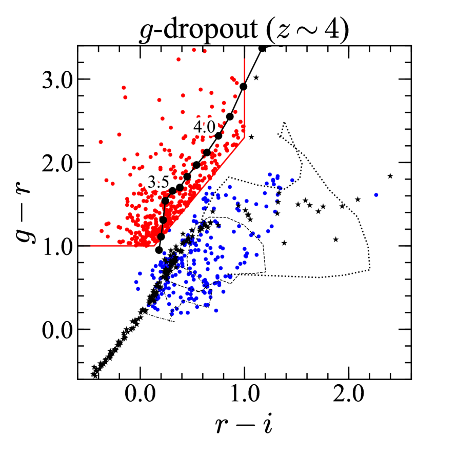
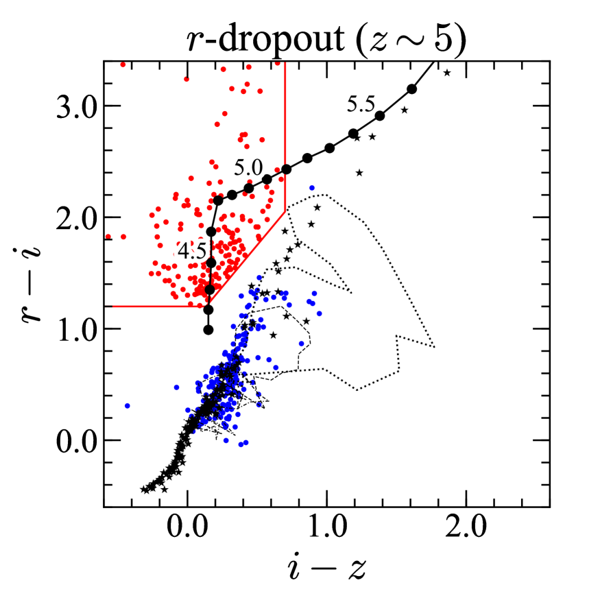
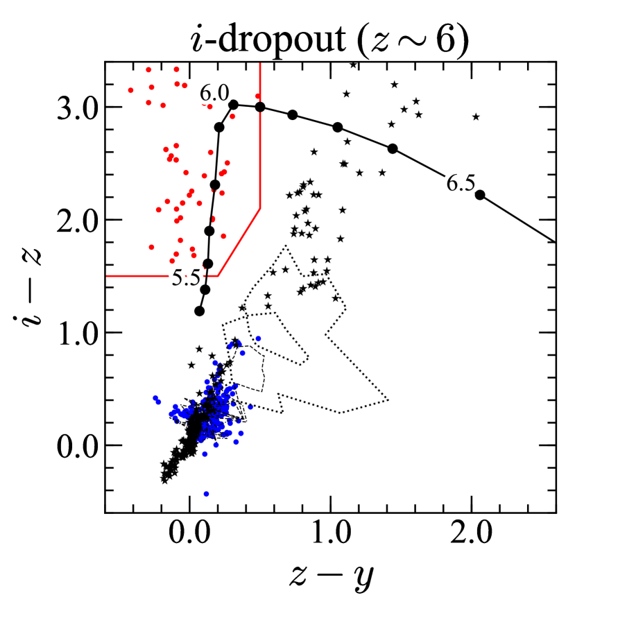
Figure 1.— Two-color diagrams to select dropout sources. The left, middle, and right panels show two-color diagrams to select $g$-dropout ($z\sim 4$), $r$-dropout ($z\sim 5$), and $i$-dropout ($z\sim 6$) sources, respectively. The red lines indicate color criteria we use to select dropout sources (Equations (1)-(9)), and the red circles are spectroscopically-identified sources in the UltraDeep layers (for the left panel) and in all layers (for the middle and right panels). The solid black lines are colors of star forming galaxies expected from the Bruzual & Charlot (2003) model as a function of redshift. As model parameters, we adopt the Salpeter (1955) IMF, an age of $70$ Myr after the initial star formation, metallicity of $Z/Z_{\odot}=0.2$, and the Calzetti et al. (2000) dust extinction law with reddening of $E(B-V)=0.16$ (see Section 3.2). The circles on the line show their redshifts with an interval of $\Delta z=0.1$. The blue circles are $z=0-3$ sources spectroscopically identified in the UD-COSMOS region. The dotted, dashed, and dot-dashed lines are, respectively, typical spectra of elliptical, Sbc, and irregular galaxies (Coleman et al. 1980) redshifted from $z=0$ to $z=2$ (for the left panel) and to $z=3$ (for the middle and right panels). The black stars indicate Galactic stars taken from Gunn & Stryker (1983) and L /T dwarfs from Knapp et al. (2004).

In addition to the observations described above, we include results of our observations with the Inamori Magellan Areal Camera and Spectrograph (IMACS; Dressler et al. 2011) on the Magellan I Baade telescope in 2007 – 2011 (PI: M. Ouchi). The IMACS observations were carried out on 2007 November 11–14, 2008 November 29–30, December 1–2, December 18–20, 2009 October 11–13, 2010 February 8–9, July 9–10, and 2011 January 3–4. In these observations, main targets were high redshift LAE candidates found in the deep Subaru Suprime-Cam narrowband images obtained in the SXDS (Ouchi et al. 2008, 2010) and COSMOS fields (Murayama et al. 2007; Shioya et al. 2009). High redshift dropout galaxy candidates selected from deep broadband images in these two fields (Furusawa et al. 2008; Capak et al. 2007) were also observed as mask fillers. The data were reduced with the Carnegie Observatories System for MultiObject Spectroscopy (cosmos) pipeline.

3. Sample Selection

3.1. Source Selection at $z\sim 4-7$

From the source catalogs made in Section 2.1, we construct $z\sim 4-7$ dropout candidate catalogs based on the Lyman break color selection technique (e.g., Steidel et al. 1996; Giavalisco 2002). As shown in Figure 1, galaxy candidates can be selected based on their $gri$, $riz$, $izy$, and $zy$ colors at $z\sim 4$, $5$, $6$, and $7$, respectively.

First, to identify secure sources, we select sources whose signal-to-noise (SN) ratios are higher than $5$ within $1.$​​″$5$-diameter apertures in the $i$-band for $g$-dropouts and in the $z$-band for $r$-dropouts. For $i$-dropouts, we select sources with signal-to-noise ratios higher than $5$ and $4$ in the $z$ and $y$-bands, respectively, because the $y$-band images are relatively shallow. For the $z$-dropouts, we select sources with signal-to-noise ratios higher than $5$ in the $y$-band. We then select dropout galaxy candidates by using their broadband spectral energy distribution (SED) colors. Like our previous studies (Ono et al. 2018; Harikane et al. 2018a; Toshikawa et al. 2018), we adopt the following color criteria:
$g$-dropouts ($z\sim 4$)

$$(g-r > 1.0)\land$$ (1)

$$(r-i < 1.0)\land$$ (2)

$$(g-r > 1.5(r-i)+0.8),$$ (3)

$r$-dropouts ($z\sim 5$)

$$(r-i > 1.2)\land$$ (4)

$$(i-z < 0.7)\land$$ (5)

$$(r-i > 1.5(i-z)+1.0),$$ (6)

$i$-dropouts ($z\sim 6$)

$$(i-z > 1.5)\land$$ (7)

$$(z-y < 0.5)\land$$ (8)

$$(i-z > 2.0(z-y)+1.1),$$ (9)

$z$-dropouts ($z\sim 7$)

$$z-y > 1.6.$$ (10)

As shown in Figure 1, these color criteria are set to avoid low redshift galaxies and stellar contaminants. Although only the $z-y$ color is used in the $z$-dropout selection, we can efficiently select $z\sim 7$ sources with this strict color criterion, as shown in previous studies similarly using the $z-y$ color (e.g., Ouchi et al. 2009).

To remove foreground interlopers, we exclude sources with continuum detections at $>2\sigma$ levels in the $g$-band for $r$-dropouts, in the $g$- or $r$-bands for $i$-dropouts, and in the $g$, $r$, or $i$-bands for $z$-dropouts, using the $1.$​​″$5$ diameter aperture magnitudes. Since our $z$-dropout candidates are detected only in $y$-band images, we carefully check coadd and single epoch observation images of the selected candidates to remove spurious sources and moving objects.

Table 3Number of Sources in Galaxy Samples Used in This Work.

Field	BM†	BX†	$U$-drop†	$g$-drop∗	$r$-drop∗	$i$-drop∗	$z$-drop∗
	$z\sim 1.7$	$z\sim 2.2$	$z\sim 3$	$z\sim 4$	$z\sim 5$	$z\sim 6$	$z\sim 7$
UltraDeep (UD)
UD-SXDS	$49184$	$20292$	$36769$	$15282$	$1517$	$59$	$8$
UD-COSMOS	$60726$	$26139$	$59838$	$10067$	$2760$	$212$	$27$
Deep (D)
D-XMM-LSS	$286685$	$110755$	$185555$	$6919$	$1237$	$5$	$1$
D-COSMOS	$192809$	$81284$	$160028$	$32602$	$6439$	$114$	$15$
D-ELAIS-N1	$172950$	$85458$	$172735$	$40815$	$3947$	$61$	$9$
D-DEEP2-3	$173450$	$81541$	$165561$	$28725$	$3808$	$131$	$13$
Wide (W)
W-W02	$\cdots$	$\cdots$	$\cdots$	$150775$	$8034$	$158$	$26$
W-W03	$\cdots$	$\cdots$	$\cdots$	$357845$	$29758$	$549$	$52$
W-W04	$\cdots$	$\cdots$	$\cdots$	$550136$	$35440$	$410$	$53$
W-W05	$\cdots$	$\cdots$	$\cdots$	$473160$	$35105$	$757$	$60$
W-W06	$\cdots$	$\cdots$	$\cdots$	$164936$	$11166$	$110$	$27$
W-W07	$\cdots$	$\cdots$	$\cdots$	$4982$	$148$	$1$	$1$
Total($z$)	$935804$	$405469$	$780486$	$1836244$	$139359$	$2567$	$292$
Total	4100221

Using the selection criteria described above, we select a total of 1,978,462 dropout candidates at $z\sim 4-7$, consisting of 1,836,244 $g$-dropouts, 139,359 $r$-dropouts, 2,567 $i$-dropouts, and $292$ $z$-dropouts. Our sample is selected from the $307.9\ \mathrm{deg^{2}}$ wide area data corresponding to a $5.92\ \mathrm{Gpc^{3}}$ survey volume, and is the largest sample of the high-redshift ($z\gtrsim$4) galaxy population to date. Especially, combined with $z\sim 2-3$ galaxies selected later in Section 3.5, we have a total of $4,100,221$ galaxies at $z\sim 2-7$, which is the largest among high redshift galaxy studies. Table 3 summarizes the number of dropout candidates in each field, and Figure 2 shows examples of sky distributions of the dropouts. The differences in the numbers of the selected candidates mainly come from the differences in the survey areas and depths.

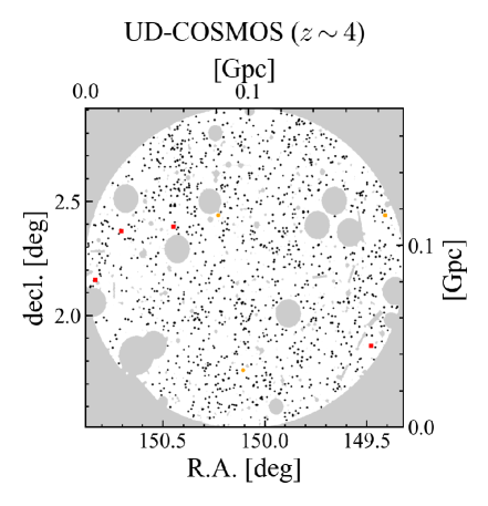
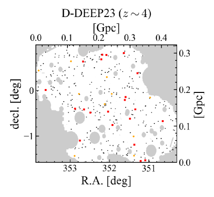
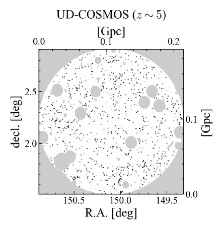
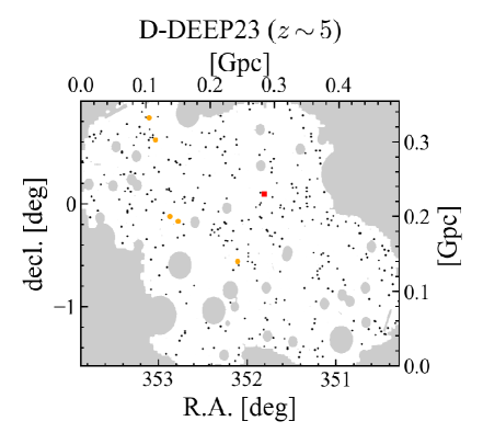
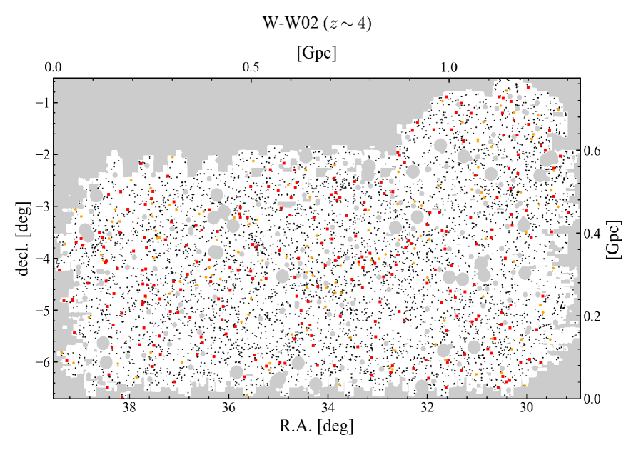
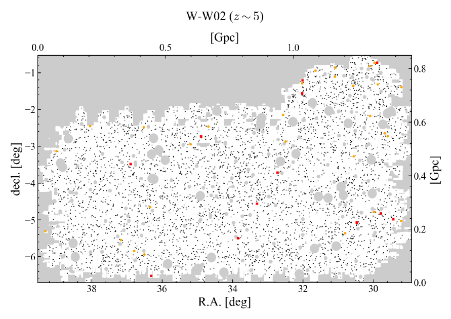
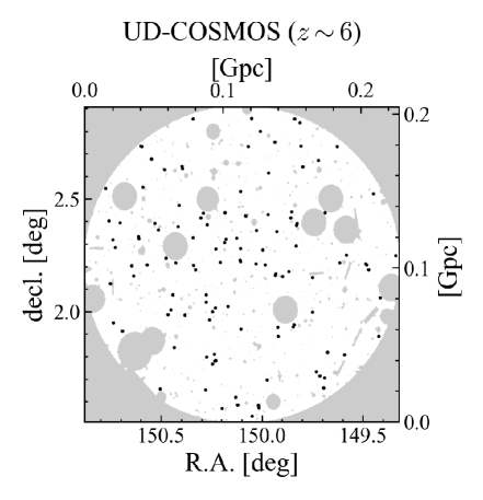
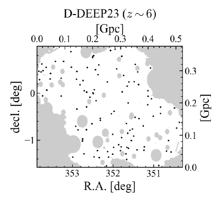
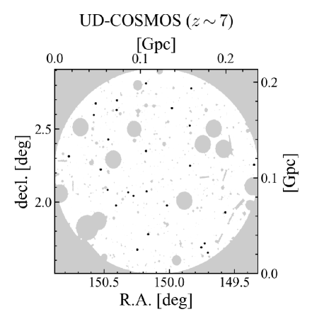
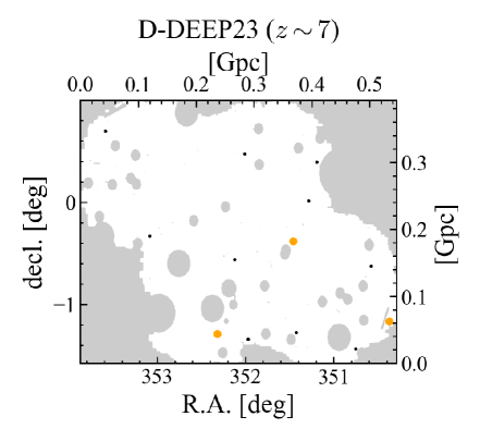
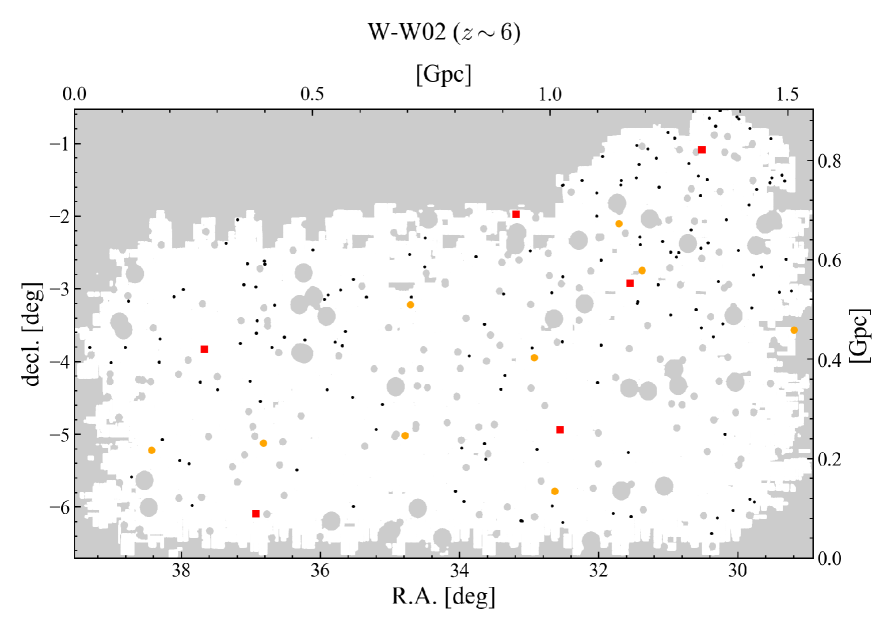
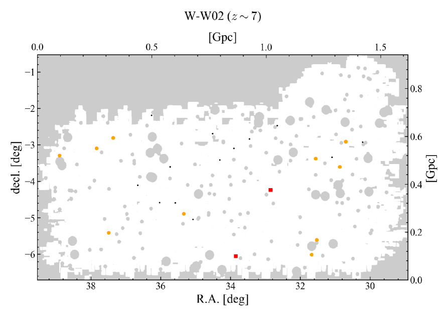
Figure 2.— Examples of sky distributions of dropout sources. The red squares, orange circles, and black dots are, respectively, the positions of sources whose magnitudes are $i<22.0$, $22.0-22.5$, and $22.5-25.0\ (24.0)$ mag for $z\sim 4$ sources, $z<22.5$, $22.5-23.0$, and $23.0-25.5\ (24.5)$ mag for $z\sim 5$ sources, and $y<23.0$, $23.0-23.5$, and $23.5-25.5\ (25.0)$ mag for $z\sim 6$ and $7$ sources, in the UltraDeep (Deep and Wide) layers. The scale on the map is marked in degrees and in the projected distance (comoving Gpc).

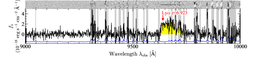
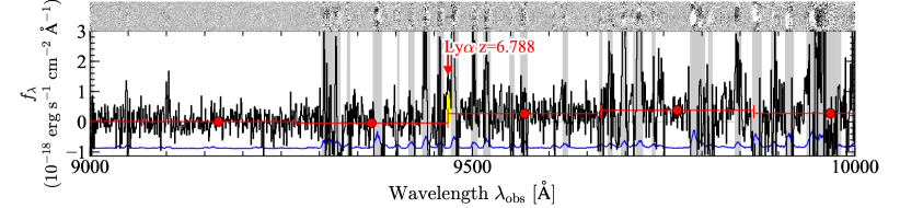
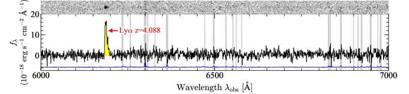
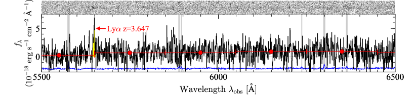
Figure 3.— Spectra of HSC J160953$+$532821 at $z=6.923$, HSC J161207$+$555919 at $z=6.788$, HSC J020834$-$021239 at $z=4.088$, and HSC J022552$-$054439 at $z=3.647$ from top to bottom, obtained in our spectroscopic follow-up observations. In each figure, the top panel shows the two-dimensional spectrum (black is positive) and the bottom panel shows the one-dimensional spectrum. In the top panel, our dropout galaxy is located at the center in the spatial direction, and the spatial range is $\pm 3\arcsec$. In the bottom panel, the black line indicates the spectrum of the object, and the blue line shows the sky spectrum with an arbitrary normalization. For the sources with weak Ly$\alpha$ emission, we also plot the averaged spectra over 200 $\mathrm{\AA}$ bins with red filled circles to show the Lyman break features.

3.2. Spectroscopically-Identified Sources

In our samples, a total of 46 sources are identified as $z>3$ objects through our spectroscopic follow-up observations with DEIMOS, AAOmega+2dF, and FOCAS (Section 2.3). Redshifts are determined based on the Ly$\alpha$ line and/or Lyman break. Figure 3 shows examples of spectroscopically identified sources, HSC J160953$+$532821, HSC J161207$+$555919, HSC J020834$-$021239, and HSC J022552$-$054439. HSC J160953$+$532821 is a faint quasar at $z=6.923$ with a UV magnitude of $M_{\mathrm{UV}}=-22.7$ mag, confirmed in our FOCAS observations. This source is also identified in Matsuoka et al. (2019). An FWHM of its Ly$\alpha$ line is $\sim 2500\ \mathrm{km\ s^{-1}}$, and a rest-frame Ly$\alpha$ equivalent width (EW) is $EW_{\mathrm{Ly\alpha}}^{0}\sim 600\ \mathrm{\AA}$. HSC J161207$+$555919 is a bright ($M_{\mathrm{UV}}=-23.0$ mag) galaxy at $z=6.788$ with a narrow Ly$\alpha$ emission line of $<300\ \mathrm{km\ s^{-1}}$ and $EW_{\mathrm{Ly\alpha}}^{0}\sim 3\ \mathrm{\AA}$, confirmed in our FOCAS observations. This source is identified as a narrow-line quasar in Matsuoka et al. (2019). The Lyman break feature can be seen in the spectrum, whose redshift is consistent with that derived from the Ly$\alpha$ emission line. HSC J020834$-$021239 and HSC J022552$-$054439 are bright galaxies at $z=4.088$ and $3.647$ identified in our DEIMOS observations, with $M_{\mathrm{UV}}=-22.7$ and $-21.8$ mag, FWHMs of 250 and 180 $\mathrm{km\ s^{-1}}$, and $EW_{\mathrm{Ly\alpha}}^{0}\sim 40$ and $9\ \mathrm{\AA}$, respectively.

In addition, we incorporate results of our spectroscopic observations for high redshift galaxies with Magellan/IMACS. We also check spectroscopic catalogs in other studies (Cuby et al. 2003, Ouchi et al. 2008, Saito et al. 2008, Willott et al. 2009, Willott et al. 2010, Curtis-Lake et al. 2012, Mallery et al. 2012, Masters et al. 2012, Le Fèvre et al. 2013, Willott et al. 2013, Kriek et al. 2015, Bañados et al. 2016, Hu et al. 2016, Matsuoka et al. 2016, Momcheva et al. 2016, Toshikawa et al. 2016, Wang et al. 2016, Hu et al. 2017, Jiang et al. 2017, Masters et al. 2017, Tasca et al. 2017, Yang et al. 2017, Hasinger et al. 2018, Matsuoka et al. 2018a, Matsuoka et al. 2018b, Ono et al. 2018, Pâris et al. 2018, Pentericci et al. 2018, Shibuya et al. 2018b, Matsuoka et al. 2019, Harikane et al. 2020b, Harikane et al. 2020a, Zhang et al. 2020, Endsley et al. 2021, and Garilli et al. 2021). We adopt their classifications between galaxies and AGNs in their catalogs, which are mostly based on apparent AGN features such as broad emission lines. For the catalogs of the VIMOS VLT Deep Survey (VVDS; Le Fèvre et al. 2013) and the VIMOS Ultra Deep Survey (VUDS; Tasca et al. 2017), we take into account sources whose reliabilities of the redshift determinations are $>70-75$%, i.e., sources with redshift reliability flags of 2, 3, 4, 9, 12, 13, 14, and 19. Here we focus on sources with spectroscopic redshifts of $z_{\rm spec}>3$ in these catalogs.

In total, 1037 dropouts in our sample have been spectroscopically identified at $z_{\rm spec}\geq 3$ in our observations and previous studies, including 770 galaxies and 267 AGNs. These sources are listed in Table 10, and the redshift distributions of the sources are shown in Figure 4. Figure 1 shows the distributions of the spectroscopically identified sources at $z_{\rm spec}>3$ in the two-color diagrams. We also plot sources in the UD-COSMOS field with spectroscopic redshifts of $z_{\rm spec}<3$ as foreground interlopers. In addition, the tracks of model spectra of young star-forming galaxies that are produced with the stellar population synthesis code galaxev (Bruzual & Charlot 2003) are shown. As model parameters, the Salpeter (1955) IMF, an age of $70$ Myr after the initial star formation, and metallicity of $Z/Z_{\odot}=0.2$ are adopted. We use the Calzetti et al. (2000) dust extinction law with reddening of $E(B-V)=0.16$. The IGM absorption is considered following the prescription of Madau (1995). The colors of the spectroscopically identified galaxies are broadly consistent with those expected from the model spectra.

3.3. Selection Completeness and Redshift Distribution

The selection completeness and redshift distributions of dropout candidates at $z\sim 4-7$ are estimated based on results of Monte Carlo simulations in Ono et al. (2018). Ono et al. (2018) run a suite of Monte Carlo simulations with an input mock catalog of high redshift galaxies with the size distribution of Shibuya et al. (2015), the Sersic index of $n=1.5$, the intrinsic ellipticities of $0.0$–$0.8$. To produce galaxy SEDs, the stellar population synthesis model of galaxev (Bruzual & Charlot 2003) is used with the Salpeter (1955) IMF, a constant rate of star formation, age of $25$ Myr, metallicity of $Z/Z_{\odot}=0.2$, and the Calzetti et al. (2000) dust extinction ranging from $E(B-V)=0.0$–$0.4$, corresponding to the UV spectral slope of $-3\lesssim\beta_{\mathrm{UV}}\lesssim-1$. We do not include Ly$\alpha$ emission in the galaxy SEDs because the line fluxes are typically not significant compared to the continuum in the broadband fluxes. The IGM attenuation is taken into account by using the prescription of Madau (1995). Different simulations are carried out for the Wide, Deep, and UltraDeep layers by using the SynPipe software (Huang et al. 2018), which utilizes GalSim v1.4 (Rowe et al. 2015) and the HSC pipeline hscpipe (Bosch et al. 2018). We insert large numbers of artificial sources into HSC images. Then we select high redshift galaxy candidates with the same selection criteria, and calculate the selection completeness as a function of magnitude and redshift, $C(m,z)$, averaged over UV spectral slope $\beta_{\mathrm{UV}}$ weighted with the $\beta_{\mathrm{UV}}$ distribution of Bouwens et al. (2014). Then the obtained completeness is scaled based on the limiting magnitudes to correct for differences in depths of the S18A data in this study and S16A data used in Ono et al. (2018).

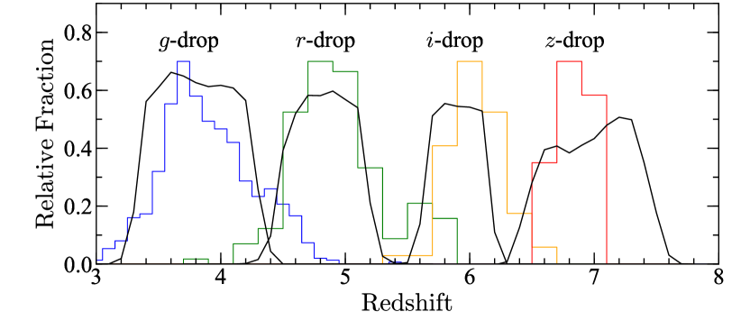
Figure 4.— Selection completeness estimates for our $z\sim 4$, $5$, $6$, and $7$ samples. The black curves correspond to the results of the Monte Carlo calculations in Section 3.3 averaged over the Wide, Deep, and UltraDeep layers. Average redshifts of these samples are 3.8, 4.9, 5.9, and 6.9. The histograms show redshift distributions of spectroscopically identified sources in the $z\sim 4$ (blue), $z\sim 5$ (green), $z\sim 6$ (orange), and $z\sim 7$ (red) samples.

Figure 4 shows results of the selection completeness estimates as a function of redshift. The average redshift values are roughly ${\bar{z}}=3.8$ for $g$-dropouts, ${\bar{z}}=4.9$ for $r$-dropouts, ${\bar{z}}=5.9$ for $i$-dropouts, and ${\bar{z}}=6.9$ for $z$-dropouts. In Figure 4, we also show the redshift distributions of the spectroscopically identified galaxies in our samples (Section 3.2). The redshift distributions of the spectroscopically identified sources are broadly consistent with the results of our selection completeness simulations. However, the distributions of the spectroscopically identified sources in the $g$-, $r$-, and $i$-dropout samples appear to be shifted toward slightly higher redshifts compared to the simulation results. This is probably because the spectroscopically identified sources are biased to ones with strong Ly$\alpha$ emission in the $g$- and $r$-dropout samples, and ones identified in the SHELLQs project searching for $z\sim 6-7$ quasars (e.g., Matsuoka et al. 2016) in the $i$-dropout sample. In particular, the redshift distribution of the spectroscopically identified $r$-dropouts has a secondary peak at $z\sim 5.7$, which is caused by $z=5.7$ Ly$\alpha$ emitters found in the Subaru Suprime-Cam and HSC narrowband surveys in the literature (e.g., Ouchi et al. 2008; Shibuya et al. 2018b). Another possible reason is the systematic uncertainty of the IGM attenuation model in the simulations. The model of Madau (1995) predicts lower redshift dropouts than Inoue et al. (2014), which may explain the discrepancy. For the $z$-dropout sample, the redshift distribution of the spectroscopically identified sources is shifted to the lower redshift, because of the increasing fraction of the neutral hydrogen at $z>7$, which resonantly scatters Ly$\alpha$ photons.

3.4. Contamination

Some foreground objects such as red galaxies at low redshifts can satisfy our color selection criteria due to photometric scatters, although intrinsically they do not enter the color selection window. This happens especially in the Wide and Deep layers, whose limiting magnitudes are relatively shallow. We evaluate contamination fractions in our dropout samples with the following three methods.

The first method is the one using estimates of photometric redshifts. We use photometric redshifts estimated with the MIZUKI code (Tanaka 2015; Tanaka et al. 2018). Here a foreground interloper is defined as a source whose 95% upper bound of the photometric redshift is less than $z=2$. We derive the fraction of the foreground interlopers as a function of the $i$- ($z$-) band magnitude in our $z\sim 4$ ($z\sim 5$) dropout samples in the Wide and Deep layers. The derived contamination fractions are presented in Table 4. In the UltraDeep layer, the fractions of the interlopers in our $z\sim 4-5$ samples are negligibly small ($<10\%$) at $m_{\mathrm{UV}}\geq 25$ mag. The contamination fraction becomes higher for brighter sources at $\lesssim 24$ mag, because the number density of high redshift galaxies decreases to brighter magnitudes, while that of foreground interlopers (e.g., low redshift passive galaxies) does not significantly change (e.g., Muzzin et al. 2013). We do not derive the contamination fraction of the $z\sim 6-7$ sources with the MIZUKI code, because accuracies of the photometric redshifts are not high due to the limited number of available bands redder than the Lyman break. In the UD-COSMOS field, we also check photometric redshifts in the COSMOS 2015 catalog (Laigle et al. 2016) that are determined with multi-band photometric data including near-infrared images such as Spizter/IRAC, useful to eliminate stellar contaminants (Stevans et al. 2018). We match our dropout sources with the COSMOS 2015 catalog within a $1\arcsec$ search radius of the object coordinate. For bright $z\sim 4-5$ sources detected with $>10\sigma$ significance levels in the HSC $i$-band, whose flux measurements are reliable, typically less than $20\%$ of them are classified as foreground interlopers, consistent with the estimates of the MIZUKI code. For fainter sources at $z\sim 4-5$, about $\sim 70\%$ of them are classified as $z>3$ galaxies. The contamination rate for $z\sim 6-7$ sources is less than $40\%$, although the number of sources is small and their flux measurements have relatively large uncertainties due to their faintness compared to the bright $z\sim 4-5$ sources. Stellar templates are also fitted for the sources in the COSMOS 2015 catalog, and only 3.5% of them are classified as stars with $\chi^{2}_{\mathrm{star}}<\chi^{2}_{\mathrm{galaxy}}$ (see Laigle et al. 2016). We also check the COSMOS Hubble ACS catalog (Leauthaud et al. 2007), and only 3.7% of them are point sources with the SExtractor (Bertin & Arnouts 1996) stellarity parameters of $>0.9$ (1=star; 0=galaxy). These analyses indicate that the fraction of the stellar contamination is negligibly small.

Table 4Estimated Contamination Fraction for the $z\sim 4$ and $z\sim 5$ Samples in UltraDeep (UD), Deep (D), and Wide (W) Layers

Redshift	$m_{\mathrm{UV}}$	Fraction (UD)	Fraction (D)	Fraction (W)
$z\sim 4$	22.0	$\cdots$	$0.69^{+0.06}_{-0.06}$	$0.60^{+0.07}_{-0.07}$
	23.0	$0.33^{+0.15}_{-0.15}$	$0.64^{+0.03}_{-0.03}$	$0.61^{+0.03}_{-0.03}$
	24.0	$0.12^{+0.06}_{-0.06}$	$0.18^{+0.02}_{-0.02}$	$0.20^{+0.02}_{-0.02}$
	24.5	$0.05^{+0.04}_{-0.04}$	$0.07^{+0.01}_{-0.01}$	$0.11^{+0.01}_{-0.01}$
	25.0	$0.02^{+0.02}_{-0.02}$	$0.04^{+0.01}_{-0.01}$	$0.08^{+0.01}_{-0.01}$
	25.5	$0.02^{+0.02}_{-0.02}$	$0.03^{+0.01}_{-0.01}$	$0.05^{+0.01}_{-0.01}$
	26.0	$0.03^{+0.01}_{-0.01}$	$0.03^{+0.01}_{-0.01}$	$0.04^{+0.01}_{-0.01}$
	26.5	$0.02^{+0.03}_{-0.03}$	$0.02^{+0.03}_{-0.03}$	$0.04^{+0.19}_{-0.19}$
$z\sim 5$	23.0	$\cdots$	$0.55^{+0.11}_{-0.11}$	$0.45^{+0.10}_{-0.10}$
	24.0	$0.02^{+0.21}_{-0.21}$	$0.35^{+0.04}_{-0.04}$	$0.35^{+0.04}_{-0.04}$
	24.5	$0.03^{+0.09}_{-0.09}$	$0.13^{+0.03}_{-0.03}$	$0.15^{+0.03}_{-0.03}$
	25.0	$0.03^{+0.05}_{-0.05}$	$0.08^{+0.02}_{-0.02}$	$0.09^{+0.02}_{-0.02}$
	25.5	$0.04^{+0.03}_{-0.03}$	$0.07^{+0.02}_{-0.02}$	$0.08^{+0.02}_{-0.02}$
	26.0	$0.06^{+0.04}_{-0.04}$	$0.06^{+0.03}_{-0.03}$	$0.06^{+0.06}_{-0.06}$
	26.5	$0.06^{+0.11}_{-0.11}$	$0.06^{+0.11}_{-0.11}$	$\cdots$

Note. — These contamination fractions are estimated based on the photometric redshift analysis (the first method in Section 3.4).

The second method is the one using the spectroscopic redshift catalog created in Section 2.3. We estimate the contamination fraction in the $z\sim 4$ sample using the results in our AAOmega+2dF spectroscopy and the VVDS spectroscopy, which target a sufficient number of bright $z\sim 4$ sources, and whose target selections are not significantly biased to low or high redshift sources. Foreground interlopers are identified based on continuum emission bluewards of the expected wavelength of the Lyman break, and/or rest-frame optical emission lines. At $z\gtrsim 5$, we cannot derive robust contamination fractions because of the small number of spectroscopically confirmed sources in the AAOmega+2dF and VVDS data. Nonetheless, we find that a total of 80 sources from our $z\sim 6-7$ dropout samples ($y=21.0-25.6$ mag) are spectroscopically identified in the entire spectroscopic catalog, and all of them are at $z_{\mathrm{spec}}>5$, although it is possible that the actual contamination rate is higher than inferred from these numbers due to various biases including the publication bias and the fact that spectroscopic observations usually prioritize the most promising candidates.

The third method is a simulation with shallower data, in the same manner as Ono et al. (2018). We use a shallower dataset whose depth is comparable with that of the Wide layer in the UD-COSMOS field, the Wide-layer-depth COSMOS data. We assume that the UD-COSMOS data are sufficiently deep and the contamination fraction in our dropout selections is small. First, we select objects that do not satisfy our selection criteria at each redshift from the UD-COSMOS catalog. Then, we find the closest source in the Wide-layer-depth COSMOS catalog that matches within a $1\arcsec$ search radius of the object coordinate. If the objects satisfy our selection criteria for the Wide-layer dropout, we regard them as foreground interlopers, and calculate their number densities. Based on comparisons between the surface number densities of interlopers and those of the selected dropouts, we estimate the fractions of foreground interlopers that satisfy our color selection criteria due to the photometric scatters. The estimated contamination fractions are $\sim 0-40\%$ for sources with $24-25$ mag at $z\sim 4-5$, comparable to those in Ono et al. (2018). For the $z\sim 6-7$ dropout samples, we cannot estimate the surface number densities of interlopers by adopting this method, because the number densities of such sources in the shallower depth COSMOS field data are too small due to the limited survey area of the UD-COSMOS field.

We find that the three methods above give the contamination fractions consistent with each other within their uncertainties at $z\sim 4-5$. As the contamination fractions used in derivations of luminosity functions later, we adopt the fractions determined based on the photometric redshifts, given their high accuracies compared to those of the other methods. For the $z\sim 4-5$ samples in the UltraDeep layer and the $z\sim 6-7$ samples, we assume that contamination fractions are negligibly small based on the results of the photometric and spectroscopic redshifts.

3.5. Source Selection at $z\sim 2-3$

In addition to the $z\sim 4-7$ catalogs, we also use catalogs of galaxy candidates at $z\sim 2-3$ to study clustering properties. We use BM, BX, and $U$-dropout galaxy catalogs at $z\sim 1.7$, $2.2$, and $3$ constructed in C. Liu et al. in prep. Here we briefly describe our source selection at $z\sim 2-3$. The $z\sim 2-3$ galaxy candidates are selected from a combined CLAUDS+HSC-SSP catalog made by Sawicki et al. (2019) based on hscpipe. Note that the HSC-SSP data in the combined CLAUDS+HSC-SSP catalog is based on the S16A internal data release, which is different from the S18A data release product we use for the $z\sim 4-7$ selection. As described in Section 2.2, the U-band images are obtained with two filters, the $u$ and $u^{*}$-bands. For the $u^{*}$-band filter, we adopt color criteria same as Hildebrandt et al. (2009), who select $z\sim 3$ dropout galaxies with the similar filter set to this study:
$U$-dropouts ($z\sim 3$)

$$(g-r < 1.2)\land$$ (11)

$$(u^{*}-g > 0.9)\land$$ (12)

$$(u^{*}-g > 1.5(g-r)+0.75).$$ (13)

For the BX and BM galaxies, we adopt the following color criteria, respectively:
BX ($z\sim 2.2$)

$$(g-r > -0.5)\land$$ (14)

$$(u^{*}-g > 2.57(g-r)+0.21)\land$$ (15)

$$(u^{*}-g > 0.42(g-r)+0.54)\land$$ (16)

$$((u^{*}-g < 0.9)\lor(u^{*}-g<1.5(g-r)+0.75)),$$ (17)

BM ($z\sim 1.7$)

$$(g-r > -0.5)\land$$ (18)

$$(u^{*}-g > -2.5(g-r)+0.98)\land$$ (19)

$$(u^{*}-g > 0.93(g-r)+0.12)\land$$ (20)

$$(u^{*}-g < 0.42(g-r)+0.54).$$ (21)

For the $ugr$ filter set, we define selection criteria by comparing the positions of stars in the $ugr$ and $u^{*}gr$ diagrams:
$U$-dropouts ($z\sim 3$)

$$(g-r < 1.2)\land$$ (22)

$$(u-g > 0.98)\land$$ (23)

$$(u-g > 1.99\times g-r+0.68),$$ (24)

BX ($z\sim 2.2$)

$$(g-r > -0.5)\land$$ (25)

$$(u-g > 3.07(g-r)+0.14)\land$$ (26)

$$(u-g > 0.42(g-r)+0.54)\land$$ (27)

$$((u-g < 0.9)\lor(u-g<1.5(g-r)+0.75)).$$ (28)

Selection criteria of BM galaxies for the $ugr$ filter set are the same as those for the $u^{*}gr$ filter set. Details of the selection are presented in C. Liu et al. in prep. A total of 935,804, 405,469, and 780,486 galaxy candidates are selected at $z\sim 1.7$, $2.2$, and $3$, respectively. The number densities of the selected galaxies are comparable to previous studies. The selection completeness and contamination fraction of these samples are described in C. Liu et al. in prep.

4. UV Luminosity Function

4.1. Dropout UV Luminosity Function

4.1.1 Derivation

We derive the rest-frame UV luminosity functions of $z\sim 4-7$ dropout sources by applying the effective volume method (Steidel et al. 1999). Based on the results of the selection completeness simulations in Section 3.3, we estimate the effective survey volume per unit area as a function of the apparent magnitude,

$$V_{\rm eff}(m)=\int C(m,z)\frac{dV(z)}{dz}dz,$$ (29)

where $C(m,z)$ is the selection completeness, i.e., the probability that a galaxy with an apparent magnitude $m$ at redshift $z$ is detected and satisfies the selection criteria, and $dV(z)/dz$ is the differential comoving volume as a function of redshift.

The space number densities of the dropouts that are corrected for incompleteness and contamination effects are obtained by calculating

$$\psi(m)=\left[1-f_{\mathrm{cont}}(m)\right]\frac{n_{\rm raw}(m)}{V_{\rm eff}(m)},$$ (30)

where $n_{\rm raw}(m)$ is the surface number density of selected dropouts in an apparent magnitude bin of $m$, and $f_{\rm cont}(m)$ is the contamination fraction in the magnitude bin estimated in Section 3.4. The $1\sigma$ uncertainties are calculated by taking account of the Poisson confidence limits (Gehrels 1986) on the numbers of the sources. To calculate $1\sigma$ uncertainties of the space number densities of dropouts, we consider uncertainties of the surface number densities and the contamination fractions.

We convert the number densities of dropouts as a function of apparent magnitude, $\psi(m)$, into the UV luminosity functions, $\Phi[M_{\rm UV}(m)]$, which is the number densities of dropouts as a function of rest-frame UV absolute magnitude. We calculate the absolute UV magnitudes of dropout samples from their apparent magnitudes using their averaged redshifts $\bar{z}$:

$$M_{\rm UV}=m+2.5\log(1+\bar{z})-5\log\left(\frac{d_{\rm L}(\bar{z})}{10\,{\rm pc}}\right)+(m_{\rm UV}-m),$$ (31)

where $d_{\rm L}$ is the luminosity distance in units of parsecs and $(m_{\rm UV}-m)$ is the $K$-correction term between the magnitude at rest-frame UV and the magnitude in the bandpass that we use. We define the UV magnitude, $m_{\mathrm{UV}}$, as the magnitude at the rest-frame $1500\ \mathrm{\AA}$. For the apparent magnitude $m$, we use a magnitude in a band whose central wavelength is the nearest to the rest-frame wavelength of $1500\ \mathrm{\AA}$, namely $i$-, $z$-, $y$-, and $y$-bands for $g$-, $r$-, $i$-, and $z$-dropouts, respectively. We set the $K$-correction term to be $0$ by assuming that dropout galaxies have flat UV continua, i.e., constant $f_{\nu}$ in the rest-frame UV ($m_{\mathrm{UV}}=m$). Note that this assumption does not have a significant impact on the calculated UV magnitudes. If we vary the UV slope ($\beta_{\mathrm{UV}}$) with $-2.5<\beta_{\mathrm{UV}}<-1.5$ (Bouwens et al. 2014), the calculated UV magnitude differs only within 0.1 mag.

4.1.2 Results

The top panel of Figure 5 shows our derived luminosity function for $g$-dropouts at $z\sim 4$ with previous studies. Our measurements have smaller error bars compared to Ono et al. (2018) because of the improved constraint on the contamination fraction (Section 3.4). Our measurements agree well with previous studies of quasars at $M_{\mathrm{UV}}\lesssim-24$ (e.g., Akiyama et al. 2018), studies of galaxies at $M_{\mathrm{UV}}\gtrsim-22$ (e.g., Bouwens et al. 2021; Finkelstein et al. 2015b), and studies of galaxies and AGNs (Ono et al. 2018; Stevans et al. 2018; Adams et al. 2020).

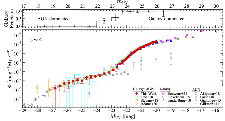
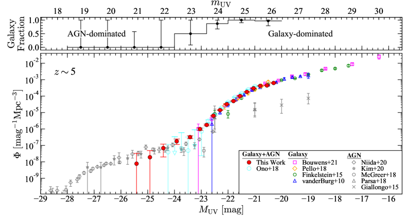
Figure 5.— Each bottom panel shows rest-frame UV luminosity functions of dropout sources (including galaxies and AGNs) at $z\sim 4$ and $5$. The red circles show our results based on the HSC-SSP survey data. For comparison, we also show previous results for galaxies+AGNs in Ono et al. (2018, cyan circles), Stevans et al. (2018, orange squares), and Adams et al. (2020, orange diamonds), galaxies in Bouwens et al. (2021, magenta squares), Finkelstein et al. (2015b, green circles), van der Burg et al. (2010, blue triangles), and Pelló et al. (2018, orange diamonds), and AGNs in Akiyama et al. (2018, black squares), Parsa et al. (2018, black triangles), Giallongo et al. (2015, black crosses), Glikman et al. (2011, black pluses), Niida et al. (2020, black diamonds), and Kim et al. (2020, black stars). Each top panel shows a fraction of galaxies in our dropout sample based on spectroscopic results. For the denominator of the fraction, the sum of the numbers of galaxies and AGNs is used. Note that this fraction is estimated based on various spectroscopic catalogs, and its uncertainty is discussed in Section 4.2.1.

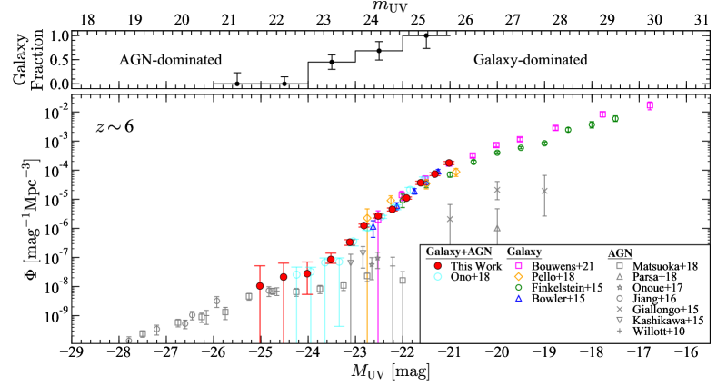
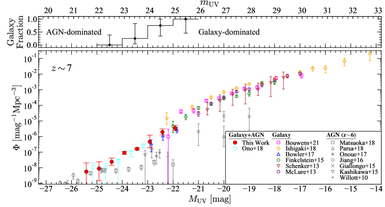
Figure 6.— Same as Figure 5 but at $z\sim 6$ and $7$. For comparison, we also show previous results for galaxies+AGNs in Ono et al. (2018, cyan circles), galaxies in Bouwens et al. (2021, magenta squares), Pelló et al. (2018, orange diamonds), Ishigaki et al. (2018, orange diamonds), Bowler et al. (2017, 2015, blue triangles), Finkelstein et al. (2015b, green circles), Schenker et al. (2013, brown triangles), and McLure et al. (2013, purple circles), and AGNs in Matsuoka et al. (2018c, black squares), Parsa et al. (2018, black triangles), Onoue et al. (2017, black stars), Jiang et al. (2016, black circles), Giallongo et al. (2015, black crosses), Kashikawa et al. (2015, black triangles), and Willott et al. (2010, black pluses). In the $z\sim 7$ panel, the $z\sim 6$ AGN luminosity functions are plotted because there are no results of the AGN luminosity function at $z\sim 7$.

Table 5Obtained Dropout (Galaxy+AGN) and Galaxy UV luminosity functions at $z\sim 4$, $5$, $6$, and $7$.

$M_{\mathrm{UV}}$	$\Phi$	$\Phi_{\mathrm{galaxy}}$†	$M_{\mathrm{UV}}$	$\Phi$	$\Phi_{\mathrm{galaxy}}$†
(mag)	($\mathrm{Mpc^{-3}}\ \mathrm{mag^{-1}}$)	($\mathrm{Mpc^{-3}}\ \mathrm{mag^{-1}}$)	(mag)	($\mathrm{Mpc^{-3}}\ \mathrm{mag^{-1}}$)	($\mathrm{Mpc^{-3}}\ \mathrm{mag^{-1}}$)
$z\sim 4$			$z\sim 5$
$-26.79$	$(1.47^{+1.67}_{-1.47})\times 10^{-8}$	$\cdots$	$-25.42$	$(7.70^{+25.20}_{-7.70})\times 10^{-9}$	$\cdots$
$-26.49$	$(2.82^{+2.95}_{-2.82})\times 10^{-8}$	$\cdots$	$-24.92$	$(1.90^{+2.92}_{-1.90})\times 10^{-8}$	$\cdots$
$-26.19$	$(5.03^{+4.45}_{-4.42})\times 10^{-8}$	$\cdots$	$-24.42$	$(6.84^{+5.14}_{-4.85})\times 10^{-8}$	$(2.58^{+14.68}_{-2.58})\times 10^{-9}$
$-25.89$	$(5.72^{+4.32}_{-4.25})\times 10^{-8}$	$\cdots$	$-23.92$	$(1.78^{+0.68}_{-0.64})\times 10^{-7}$	$(4.73^{+10.22}_{-4.73})\times 10^{-8}$
$-25.59$	$(9.48^{+6.03}_{-5.96})\times 10^{-8}$	$\cdots$	$-23.42$	$(3.19^{+0.65}_{-0.61})\times 10^{-7}$	$(1.57^{+2.48}_{-1.57})\times 10^{-7}$
$-25.29$	$(1.13^{+0.63}_{-0.62})\times 10^{-7}$	$\cdots$	$-23.05$	$(9.87^{+1.60}_{-1.60})\times 10^{-7}$	$(6.22^{+4.19}_{-4.19})\times 10^{-7}$
$-24.99$	$(9.75^{+4.92}_{-4.80})\times 10^{-8}$	$\cdots$	$-22.80$	$(1.76^{+0.23}_{-0.19})\times 10^{-6}$	$(1.27^{+0.67}_{-0.66})\times 10^{-6}$
$-24.69$	$(2.26^{+0.96}_{-0.96})\times 10^{-7}$	$\cdots$	$-22.55$	$(6.39^{+0.43}_{-0.43})\times 10^{-6}$	$(5.21^{+2.28}_{-2.28})\times 10^{-6}$
$-24.39$	$(2.77^{+1.04}_{-1.04})\times 10^{-7}$	$(1.11^{+2.74}_{-1.11})\times 10^{-8}$	$-22.30$	$(1.40^{+0.07}_{-0.07})\times 10^{-5}$	$(1.24^{+0.43}_{-0.43})\times 10^{-5}$
$-24.09$	$(2.92^{+0.97}_{-0.97})\times 10^{-7}$	$(4.30^{+5.65}_{-4.30})\times 10^{-8}$	$-22.05$	$(3.22^{+0.13}_{-0.13})\times 10^{-5}$	$(2.97^{+0.80}_{-0.80})\times 10^{-5}$
$-23.79$	$(3.63^{+1.06}_{-1.06})\times 10^{-7}$	$(9.22^{+9.32}_{-9.22})\times 10^{-8}$	$-21.80$	$(5.00^{+0.22}_{-0.22})\times 10^{-5}$	$(4.78^{+1.10}_{-1.10})\times 10^{-5}$
$-23.49$	$(6.01^{+1.54}_{-1.54})\times 10^{-7}$	$(2.17^{+1.83}_{-1.83})\times 10^{-7}$	$-21.55$	$(1.01^{+0.04}_{-0.04})\times 10^{-4}$	$(1.00^{+0.20}_{-0.20})\times 10^{-4}$
$-23.19$	$(8.05^{+1.17}_{-1.17})\times 10^{-7}$	$(3.63^{+2.30}_{-2.30})\times 10^{-7}$	$-21.30$	$(1.79^{+0.06}_{-0.06})\times 10^{-4}$	$(1.77^{+0.38}_{-0.38})\times 10^{-4}$
$-22.89$	$(1.49^{+0.16}_{-0.16})\times 10^{-6}$	$(8.07^{+4.28}_{-4.28})\times 10^{-7}$	$-21.05$	$(2.97^{+0.11}_{-0.11})\times 10^{-4}$	$(2.93^{+0.71}_{-0.71})\times 10^{-4}$
$-22.64$	$(2.91^{+0.30}_{-0.30})\times 10^{-6}$	$(1.97^{+0.92}_{-0.92})\times 10^{-6}$	$-20.80$	$(4.18^{+0.14}_{-0.14})\times 10^{-4}$	$(4.09^{+1.14}_{-1.14})\times 10^{-4}$
$-22.44$	$(6.72^{+0.51}_{-0.51})\times 10^{-6}$	$(5.67^{+2.01}_{-2.01})\times 10^{-6}$	$-20.55$	$(4.45^{+0.17}_{-0.17})\times 10^{-4}$	$(4.31^{+1.50}_{-1.50})\times 10^{-4}$
$-22.29$	$(9.54^{+1.11}_{-1.11})\times 10^{-6}$	$(9.24^{+4.10}_{-4.10})\times 10^{-6}$	$-20.30$	$(6.29^{+0.24}_{-0.24})\times 10^{-4}$	$(6.13^{+2.52}_{-2.52})\times 10^{-4}$
$-22.19$	$(1.53^{+0.15}_{-0.15})\times 10^{-5}$	$(1.53^{+0.61}_{-0.61})\times 10^{-5}$	$z\sim 6$
$-22.09$	$(1.90^{+0.16}_{-0.16})\times 10^{-5}$	$(1.89^{+0.68}_{-0.68})\times 10^{-5}$	$-25.02$	$(1.05^{+4.11}_{-1.05})\times 10^{-8}$	$\cdots$
$-21.99$	$(2.77^{+0.20}_{-0.20})\times 10^{-5}$	$(2.75^{+0.92}_{-0.92})\times 10^{-5}$	$-24.52$	$(2.13^{+4.21}_{-2.13})\times 10^{-8}$	$\cdots$
$-21.89$	$(3.70^{+0.24}_{-0.24})\times 10^{-5}$	$(3.66^{+1.13}_{-1.13})\times 10^{-5}$	$-24.02$	$(2.77^{+4.19}_{-2.23})\times 10^{-8}$	$(6.00^{+9.95}_{-6.00})\times 10^{-9}$
$-21.79$	$(5.52^{+0.30}_{-0.30})\times 10^{-5}$	$(5.44^{+1.58}_{-1.58})\times 10^{-5}$	$-23.52$	$(8.51^{+5.38}_{-2.25})\times 10^{-8}$	$(3.76^{+2.97}_{-2.05})\times 10^{-8}$
$-21.69$	$(7.49^{+0.36}_{-0.36})\times 10^{-5}$	$(7.38^{+1.89}_{-1.89})\times 10^{-5}$	$-23.12$	$(3.34^{+0.72}_{-0.72})\times 10^{-7}$	$(1.80^{+1.09}_{-1.09})\times 10^{-7}$
$-21.59$	$(1.04^{+0.04}_{-0.04})\times 10^{-4}$	$(1.03^{+0.23}_{-0.23})\times 10^{-4}$	$-22.82$	$(1.24^{+0.15}_{-0.14})\times 10^{-6}$	$(7.59^{+4.14}_{-4.14})\times 10^{-7}$
$-21.49$	$(1.29^{+0.05}_{-0.05})\times 10^{-4}$	$(1.28^{+0.26}_{-0.26})\times 10^{-4}$	$-22.52$	$(2.67^{+0.39}_{-0.39})\times 10^{-6}$	$(1.81^{+0.96}_{-0.96})\times 10^{-6}$
$-21.39$	$(1.84^{+0.06}_{-0.06})\times 10^{-4}$	$(1.82^{+0.34}_{-0.34})\times 10^{-4}$	$-22.22$	$(4.48^{+0.53}_{-0.53})\times 10^{-6}$	$(3.46^{+1.78}_{-1.78})\times 10^{-6}$
$-21.29$	$(2.24^{+0.07}_{-0.07})\times 10^{-4}$	$(2.23^{+0.38}_{-0.38})\times 10^{-4}$	$-21.92$	$(1.10^{+0.09}_{-0.09})\times 10^{-5}$	$(9.58^{+4.82}_{-4.82})\times 10^{-6}$
$-21.19$	$(2.93^{+0.08}_{-0.08})\times 10^{-4}$	$(2.92^{+0.49}_{-0.49})\times 10^{-4}$	$-21.62$	$(3.69^{+0.48}_{-0.48})\times 10^{-5}$	$(3.55^{+1.80}_{-1.80})\times 10^{-5}$
$-21.09$	$(3.88^{+0.17}_{-0.17})\times 10^{-4}$	$(3.86^{+0.67}_{-0.67})\times 10^{-4}$	$-21.32$	$(7.35^{+0.85}_{-0.85})\times 10^{-5}$	$(7.35^{+4.05}_{-4.05})\times 10^{-5}$
$-20.99$	$(4.61^{+0.19}_{-0.19})\times 10^{-4}$	$(4.58^{+0.81}_{-0.81})\times 10^{-4}$	$-21.02$	$(1.77^{+0.21}_{-0.21})\times 10^{-4}$	$(1.77^{+1.22}_{-1.22})\times 10^{-4}$
$-20.89$	$(5.19^{+0.20}_{-0.20})\times 10^{-4}$	$(5.16^{+0.93}_{-0.93})\times 10^{-4}$	$z\sim 7$
$-20.79$	$(6.39^{+0.22}_{-0.22})\times 10^{-4}$	$(6.35^{+1.16}_{-1.16})\times 10^{-4}$	$-25.42$	$(5.64^{+14.65}_{-5.64})\times 10^{-9}$	$\cdots$
$-20.69$	$(8.20^{+0.26}_{-0.26})\times 10^{-4}$	$(8.15^{+1.51}_{-1.51})\times 10^{-4}$	$-24.92$	$(8.89^{+15.29}_{-7.41})\times 10^{-9}$	$\cdots$
$-20.59$	$(9.14^{+0.27}_{-0.27})\times 10^{-4}$	$(9.08^{+1.72}_{-1.72})\times 10^{-4}$	$-24.42$	$(2.41^{+1.75}_{-0.98})\times 10^{-8}$	$(5.00^{+24.81}_{-5.00})\times 10^{-10}$
$-20.49$	$(1.04^{+0.03}_{-0.03})\times 10^{-3}$	$(1.03^{+0.20}_{-0.20})\times 10^{-3}$	$-23.92$	$(9.02^{+2.13}_{-1.66})\times 10^{-8}$	$(1.31^{+2.46}_{-1.31})\times 10^{-8}$
$-20.39$	$(1.20^{+0.03}_{-0.03})\times 10^{-3}$	$(1.19^{+0.24}_{-0.24})\times 10^{-3}$	$-23.42$	$(1.62^{+0.30}_{-0.23})\times 10^{-7}$	$(4.39^{+6.02}_{-4.39})\times 10^{-8}$
$-20.29$	$(1.47^{+0.04}_{-0.04})\times 10^{-3}$	$(1.46^{+0.31}_{-0.31})\times 10^{-3}$	$-22.92$	$(4.63^{+7.53}_{-2.71})\times 10^{-7}$	$(1.83^{+3.62}_{-1.83})\times 10^{-7}$
$-20.19$	$(1.60^{+0.04}_{-0.04})\times 10^{-3}$	$(1.59^{+0.36}_{-0.36})\times 10^{-3}$	$-22.42$	$(1.95^{+1.13}_{-0.67})\times 10^{-6}$	$(1.06^{+1.20}_{-1.06})\times 10^{-6}$
$-20.09$	$(1.79^{+0.04}_{-0.04})\times 10^{-3}$	$(1.78^{+0.44}_{-0.44})\times 10^{-3}$	$-21.92$	$(3.47^{+1.70}_{-1.03})\times 10^{-6}$	$(2.75^{+2.77}_{-2.55})\times 10^{-6}$
$-19.99$	$(2.03^{+0.05}_{-0.05})\times 10^{-3}$	$(2.02^{+0.54}_{-0.54})\times 10^{-3}$	$\cdots$	$\cdots$	$\cdots$

Our derived luminosity functions at $z\sim 5$ and $6$ are shown in the bottom panel of Figure 5 and the top panel of Figure 6, respectively. Similar to the $z\sim 4$ result, our measurements agree well with previous studies of quasars at $M_{\mathrm{UV}}\lesssim-24$ mag (e.g., Niida et al. 2020; Matsuoka et al. 2018c), studies of galaxies at $M_{\mathrm{UV}}\gtrsim-22$ mag (e.g., Bouwens et al. 2021; Finkelstein et al. 2015b), and studies of galaxies and AGNs (Ono et al. 2018). At $z\sim 7$, our derived luminosity function agrees with previous studies (e.g., Ono et al. 2018; Bowler et al. 2017), as shown in the bottom panel of Figure 6. Table 5 summarizes our measurements of the luminosity functions at $z\sim 4-7$.

These agreements clearly indicate that the dropout luminosity function is a superposition of the AGN luminosity function (dominant at $M_{\mathrm{UV}}<-24$ mag) and the galaxy luminosity function (dominant at $M_{\mathrm{UV}}>-22$ mag). In our dropout selection, we probe redshifted Lyman break features of high redshift galaxies. However, high redshift AGNs also have similar Lyman break features. Thus it is expected that our dropout sample is composed of both galaxies and AGNs. Indeed, as described in Section 3.2, our dropout samples include both spectroscopically identified galaxies and AGNs. Based on our spectroscopic results and the literature, we derive the galaxy fraction which is the number of spectroscopically confirmed high redshift galaxies divided by the sum of the numbers of spectroscopically confirmed galaxies and AGNs. The derived galaxy fractions for our $z\sim 4-7$ samples in each magnitude bin are presented in Figures 5 and 6. As shown in Figures 5 and 6, the galaxy fractions at $z\sim 4-7$ are about $0$% at $M_{\rm UV}<-24$ mag, but then increase with increasing magnitude and reach about $100$% at $M_{\rm UV}>-22$ mag. These results further suggest that our luminosity functions are dominated by AGNs at the bright end, and by galaxies at the faint end. The very wide area and deep depth of the HSC-SSP survey allow us to bridge the UV luminosity functions of high redshift galaxies and AGNs, both of which can be selected with redshifted Lyman break features (Ono et al. 2018).

4.1.3 Fitting the Dropout Luminosity Functions

We investigate the shape of the UV luminosity functions of dropout sources (galaxies+AGNs) by fitting them with several functional forms. Figure 7 shows our UV luminosity functions at $z\sim 4-7$ with previous results of galaxies based on the Hubble data (Bouwens et al. 2021; Ishigaki et al. 2018) and of quasars based on the HSC-SSP and Sloan Digital Sky Survey (SDSS) data (Akiyama et al. 2018; Niida et al. 2020; Matsuoka et al. 2018c). The combination of our results with the previous work reveals the UV luminosity functions in a very wide magnitude range of $-29\lesssim M_{\rm UV}\lesssim-14$ mag, corresponding to the luminosity range of $0.002L^{*}_{\mathrm{UV}}\lesssim L_{\mathrm{UV}}\lesssim 2000L^{*}_{\mathrm{UV}}$. We also show luminosity functions at $z\sim 3$ taken from Moutard et al. (2020), Bouwens et al. (2021), and Zhang et al. (2021). As discussed in Section 4.1.2, the dropout luminosity function is a superposition of the AGN luminosity function and the galaxy luminosity function. Thus we simultaneously fit the AGN and galaxy luminosity functions. For the AGN luminosity function, we fit with a double-power law (DPL) function that is widely used in studies of AGNs:

$$\phi(L)dL=\phi^{*}\left[\left(\frac{L}{L^{*}}\right)^{-\alpha}+\left(\frac{L}{L^{*}}\right)^{-\beta}\right]^{-1}\frac{dL}{L^{*}},$$ (32)

where $\phi^{*}$ is the overall normalization, $L^{*}$ is the characteristic luminosity, and $\alpha$ and $\beta$ are the faint and bright-end power-law slopes, respectively. We define a DPL function as a function of absolute magnitude, $\Phi(M_{\rm UV})$, as $\phi(L)dL=\Phi(M_{\rm UV})dM_{\rm UV}$,

$$\Phi(M_{\rm UV})=\frac{\ln 10}{2.5}\phi^{*}$$

$$\times\left[10^{0.4(\alpha+1)(M_{\rm UV}-M_{\rm UV}^{*})}+10^{0.4(\beta+1)(M_{\rm UV}-M_{\rm UV}^{*})}\right]^{-1},$$ (33)

where $M^{*}_{\rm UV}$ is the characteristic magnitude. For the galaxy luminosity function, we fit with a DPL function or the Schechter function (Schechter 1976):

$$\phi(L)dL=\phi^{*}\left(\frac{L}{L^{*}}\right)^{\alpha}\exp\left(-\frac{L}{L^{*}}\right)d\left(\frac{L}{L^{*}}\right),$$ (34)

where $\phi^{*}$, $L^{*}_{\rm UV}$, and $\alpha$ are the overall normalization, the characteristic luminosity, and the faint power-law slope, respectively. We define the Schechter function as a function of absolute magnitude, $\Phi(M_{\rm UV})$, as $\phi(L)dL=\Phi(M_{\rm UV})dM_{\rm UV}$,

$$\Phi(M_{\rm UV}) = \frac{\ln 10}{2.5}\phi^{*}10^{-0.4(M_{\rm UV}-M_{\rm UV}^{*})(\alpha+1)}$$ (35)

$$\times\exp\left(-10^{-0.4(M_{\rm UV}-M_{\rm UV}^{*})}\right).$$

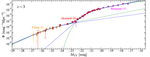
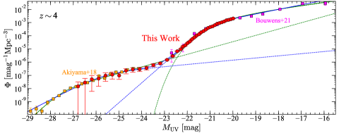
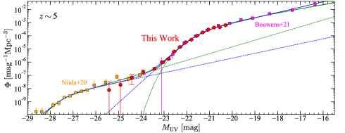
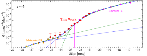
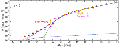
Figure 7.— Rest-frame UV luminosity functions of all rest-UV selected sources (galaxies+AGNs) at $z\sim 3$, $4$, $5$, $6$, and $7$ from top to bottom. The red circles show our results based on the HSC-SSP survey data at $z\sim 4-7$ and results in Moutard et al. (2020) at $z\sim 3$. The magenta squares and orange diamonds are results for galaxies taken from Bouwens et al. (2021) and Ishigaki et al. (2018), respectively. The orange squares are results for AGNs in Zhang et al. (2021), Akiyama et al. (2018), Niida et al. (2020), and Matsuoka et al. (2018c) at $M_{\mathrm{UV}}<-24$ mag. The blue (green) lines show the best-fit DPL+DPL (DPL+Schechter) functions. Note that at $z\sim 7$, we fix the parameters of the AGN luminosity function to values in Matsuoka et al. (2018c) with decreasing the $\phi^{*}$ parameter by 0.7 dex following $\phi^{*}\propto 10^{-0.7(z-6)}$ as assumed in Matsuoka et al. (2018c).

Figure 7 shows the best-fit results in cases of the DPL+DPL and DPL+Schechter functions at $z\sim 3-7$. Note that in the fitting at $z\sim 7$, we fix the parameters of the AGN luminosity function to values in Matsuoka et al. (2018c) with decreasing the $\phi^{*}$ parameter by 0.7 dex following $\phi^{*}\propto 10^{-0.7(z-6)}$ as assumed in Matsuoka et al. (2018c), because there are no measurements of the AGN luminosity function at $z\sim 7$. The luminosity functions in the very wide luminosity range of $-29\lesssim M_{\rm UV}\lesssim-14$ mag are well fitted with either the DPL+DPL or DPL+Schechter functions, as partly shown at $z\sim 4$ in previous studies (Stevans et al. 2018; Adams et al. 2020), except for $z\sim 7$ where the DPL+DPL functions provide a better fit. Table 6 summarizes the best-fit parameters and reduced $\chi^{2}$ values of the two cases. We find that the best-fit parameters are roughly comparable to those of galaxy and AGN luminosity functions in previous studies (e.g., Ono et al. 2018; Akiyama et al. 2018; Niida et al. 2020; Matsuoka et al. 2018c).

Table 6Fit Parameters for Luminosity Functions of All Rest-UV Selected Sources (Galaxy+AGN)

		AGN Component					Galaxy Component
Redshift	Fitted Function	$M_{\mathrm{UV}}^{*}$	$\mathrm{log}\phi^{*}$	$\alpha$	$\beta$		$M_{\mathrm{UV}}^{*}$	$\mathrm{log}\phi^{*}$	$\alpha$	$\beta$	$\chi^{2}/\mathrm{dof}$
		($\mathrm{Mpc^{-3}}$)	(mag)				($\mathrm{Mpc^{-3}}$)	(mag)
$z\sim 3^{*}$	DPL+DPL	$-24.59^{+0.25}_{-0.50}$	$-5.74^{+0.13}_{-0.26}$	$-1.59^{+0.41}_{-0.29}$	$-2.84^{+0.41}_{-0.17}$		$-21.30^{+0.05}_{-0.05}$	$-3.23^{+0.04}_{-0.04}$	$-1.89^{+0.02}_{-0.02}$	$-4.78^{+0.19}_{-0.23}$	$52.6/29$
	DPL+Schechter	$-25.31^{+1.01}_{-0.44}$	$-6.11^{+0.50}_{-0.24}$	$-1.86^{+0.43}_{-0.37}$	$-3.04^{+0.19}_{-0.19}$		$-20.91^{+0.12}_{-0.08}$	$-2.84^{+0.06}_{-0.05}$	$-1.68^{+0.08}_{-0.04}$	$\cdots$	$55.3/30$
$z\sim 4$	DPL+DPL	$-25.69^{+0.19}_{-0.10}$	$-6.74^{+0.10}_{-0.06}$	$-1.41^{+0.17}_{-0.09}$	$-3.24^{+0.06}_{-0.07}$		$-20.99^{+0.03}_{-0.03}$	$-3.00^{+0.02}_{-0.02}$	$-1.86^{+0.03}_{-0.02}$	$-4.77^{+0.05}_{-0.05}$	$127.6/64$
	DPL+Schechter	$-27.49^{+0.26}_{-0.08}$	$-8.00^{+0.20}_{-0.06}$	$-2.20^{+0.06}_{-0.03}$	$-5.05^{+0.57}_{-0.24}$		$-20.49^{+0.03}_{-0.02}$	$-2.52^{+0.02}_{-0.02}$	$-1.59^{+0.03}_{-0.03}$	$\cdots$	$115.0/65$
$z\sim 5$	DPL+DPL	$-27.32^{+0.76}_{-0.26}$	$-8.35^{+0.47}_{-0.18}$	$-1.92^{+0.31}_{-0.17}$	$-4.77^{+0.61}_{-0.62}$		$-21.54^{+0.04}_{-0.04}$	$-3.63^{+0.04}_{-0.03}$	$-2.01^{+0.04}_{-0.03}$	$-4.91^{+0.08}_{-0.08}$	$100.9/36$
	DPL+Schechter	$-27.67^{+1.47}_{-0.88}$	$-8.71^{+0.89}_{-0.67}$	$-2.27^{+0.48}_{-0.22}$	$-5.92^{+0.66}_{-1.14}$		$-21.09^{+0.04}_{-0.03}$	$-3.16^{+0.03}_{-0.03}$	$-1.76^{+0.04}_{-0.03}$	$\cdots$	$104.1/37$
$z\sim 6$	DPL+DPL	$-27.05^{+0.62}_{-0.44}$	$-9.03^{+0.28}_{-0.19}$	$-1.61^{+0.27}_{-0.23}$	$-3.41^{+0.30}_{-0.40}$		$-21.03^{+0.09}_{-0.08}$	$-3.52^{+0.09}_{-0.07}$	$-2.08^{+0.07}_{-0.06}$	$-4.57^{+0.09}_{-0.10}$	$41.5/22$
	DPL+Schechter	$-26.53^{+0.51}_{-0.74}$	$-8.83^{+0.20}_{-0.41}$	$-1.99^{+0.88}_{-0.36}$	$-2.90^{+0.14}_{-0.21}$		$-21.22^{+0.15}_{-0.12}$	$-3.65^{+0.16}_{-0.13}$	$-2.19^{+0.08}_{-0.06}$	$\cdots$	$97.4/23$
$z\sim 7$	DPL+DPL	$(-24.90)^{\dagger}$	$(-8.49)\dagger$	$(-1.23)\dagger$	$(-2.73)\dagger$		$-20.12^{+0.21}_{-0.24}$	$-3.05^{+0.15}_{-0.16}$	$-1.89^{+0.10}_{-0.09}$	$-3.81^{+0.10}_{-0.13}$	$58.6/24$
	DPL+Schechter	$(-24.90)\dagger$	$(-8.49)\dagger$	$(-1.23)\dagger$	$(-2.73)\dagger$		$-20.49^{+0.12}_{-0.10}$	$-3.14^{+0.10}_{-0.09}$	$-1.88^{+0.07}_{-0.06}$	$\cdots$	$105.2/25$

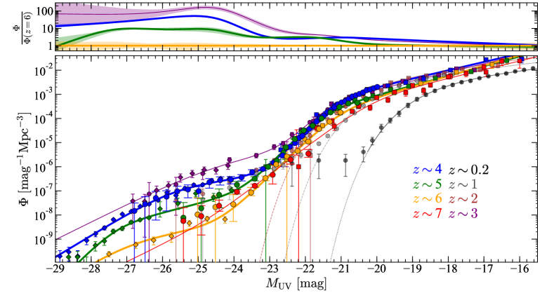
Figure 8.— Evolution of the rest-frame UV luminosity functions of all rest-UV selected sources (galaxies+AGNs) from $z\sim 7$ to $z\sim 0$. The bottom panel shows the luminosity functions at $z\sim 0-7$, and the black, grey, brown, purple, blue, green, orange, and red symbols show results at $z\sim 0.2$, $1$, $2$, $3$, $4$, $5$, $6$, and $7$, respectively. The circles at $z\sim 4-7$ show our results based on the HSC-SSP survey data, and those at $z\sim 0-3$ are taken from Moutard et al. (2020) at $0.05<z<0.3$, $0.9<z<1.3$, $1.8<z<2.5$, and $2.5<z<3.5$. The diamonds are results for AGNs in Zhang et al. (2021), Akiyama et al. (2018), Niida et al. (2020), and Matsuoka et al. (2018c) at $z\sim 3$, $4$, $5$, and $6$, respectively, and the squares show results for galaxies in Bouwens et al. (2021) and Ishigaki et al. (2018). The lines show the best-fit DPL+DPL functions at $z\sim 3-7$ (this study), and Schechter functions at $z\sim 0-2$ (Moutard et al. 2020). The top panel shows ratios of the number densities at $z\sim 3-5$ relative to those at $z\sim 6$. The shaded regions correspond to the $2\sigma$ uncertainties of the luminosity function parameters. The number density of typical galaxies ($M_{\mathrm{UV}}=M^{*}_{\mathrm{UV}}\sim-21$ mag) increases only by a factor of $\sim 3$ from $z\sim 6$ to $3$, while the number density of typical quasars ($M_{\mathrm{UV}}=M^{*}_{\mathrm{UV}}\sim-27$ mag) significantly increases by a factor of $\sim 100$.

4.1.4 Redshift Evolution

Figure 8 summarizes UV luminosity function estimates at $z\sim 4-7$ in this work and the literature, and the best-fit DPL+DPL functions. We also plot the rest-frame UV luminosity functions at $z\sim 0-3$ from Moutard et al. (2020). Like our $z\sim 4-7$ results, the luminosity functions at $z\sim 0-3$ also show number density excesses at the bright end compared to the Schechter functions, which are dominated by AGNs (see discussions in Moutard et al. 2020). Indeed, the number densities of bright sources ($M_{\mathrm{UV}}\lesssim-23$ mag) at $z\sim 3$ are comparable to the rest-frame UV luminosity function of spectroscopically identified AGNs in Zhang et al. (2021). Interestingly, the number density of typical galaxies ($M_{\mathrm{UV}}=M^{*}_{\mathrm{UV}}\sim-21$ mag) increases only by a factor of $\sim 3$ from $z\sim 6$ to $3$, while the number density of typical quasars ($M_{\mathrm{UV}}=M^{*}_{\mathrm{UV}}\sim-27$ mag) significantly increases by a factor of $\sim 100$, consistent with previous studies of the quasar luminosity functions (e.g., Matsuoka et al. 2018c; Niida et al. 2020). This indicates a very rapid growth of AGNs in the first 1.5 Gyr. If we extrapolate this evolution to higher redshift by assuming $\Phi\propto 10^{-0.7(1+z)}$ (Matsuoka et al. 2018c), the number density of bright quasars ($M_{\mathrm{UV}}\lesssim-26$ mag) will be very small ($\lesssim 2\times 10^{-10}\ \mathrm{mag^{-1}\ \mathrm{Mpc^{-3}}}$) at $z\geq 7$. More specifically, the number density of typical quasars increases by a factor of 10 from $z\sim 6$ to $5$, but increases only by a factor of 3 from $z\sim 4$ to $3$, indicating the accelerated evolution of the quasar luminosity function at $z\sim 3-6$ (Niida et al. 2020).

4.2. Galaxy UV Luminosity Function

4.2.1 Derivation and Results

We estimate the galaxy UV luminosity functions in a wide magnitude range by considering the contributions from AGNs in our dropout luminosity function measurements. To subtract the AGN contributions, we use the galaxy fraction estimates based on the spectroscopy shown in Figures 5 and 6. We multiply the dropout (galaxy+AGN) UV luminosity functions by the spectroscopic galaxy fractions, $f_{\mathrm{galaxy}}$, and obtain the galaxy luminosity functions, $\Phi_{\mathrm{galaxy}}$:

$$\Phi_{\mathrm{galaxy}}(M_{\mathrm{UV}})=f_{\mathrm{galaxy}}(M_{\mathrm{UV}})\Phi(M_{\mathrm{UV}}).$$ (36)

Note that our galaxy fraction estimates are based on various spectroscopic catalogs, and it is possible that the estimates are biased due to a variety of different spectroscopic selection functions. In order to check this possibility, we compares the estimated galaxy fractions at $z\sim 4$ with those derived from the VVDS data (Le Fèvre et al. 2013), whose targets are purely selected based on their $i$-band magnitude. As shown in Figure 9, the estimated galaxy fractions are consistent with each other within the errors, indicating that our estimates are not significantly biased. Future large spectroscopic surveys such as Subaru/Prime Focus Spectrograph (PFS) will allow us to acculately determine the spectroscopic galaxy fractions.

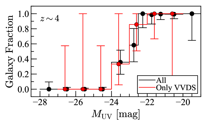
Figure 9.— Spectroscopic galaxy fraction at $z\sim 4$. The black circles are those estimated by using the all available spectroscopic catalogs (same as the top panel of Figure 5), and the red circles are those estimated with the VVDS data (Le Fèvre et al. 2013).

Figure 10 and Table 5 show our estimates of the galaxy UV luminosity functions at $z\sim 4-7$. We confirm that our results are consistent with the previous results in the UV magnitude range fainter than $-22$ mag. This is because the number density of AGNs are negligibly small compared to that of galaxies in this magnitude range. In the brighter magnitude range of $M_{\rm UV}<-23$ mag, our estimates at $z\sim 4-7$ appear to have bright end excesses of number densities compared to the exponential decline, although the uncertainties are large. The number densities of bright galaxies at $z\sim 6$ are determined more precisely than those at $z\sim 5$ thanks to the rich spectroscopic data at $z\sim 6$ mainly taken in the SHELLQs project. Note that the effect of the Eddington bias (Eddington 1913) should be small on these bright end excesses, because their magnitude ranges are much brighter than the limiting magnitudes, as discussed in Ono et al. (2018).

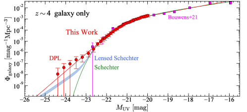
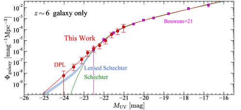
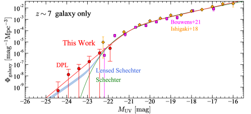
Figure 10.— Rest-frame UV luminosity functions of galaxies that take into account AGN fraction correction at $z\sim 4$, $5$, $6$, and $7$ from top to bottom. The red line is the best-fit DPL function, and the green line is the best-fit Schechter function without considering the lensing effect. The blue shaded region corresponds to the lensed Schechter functions with the two cases of optical depth estimates (Takahashi et al. 2011 and Barone-Nugent et al. 2015). The red circles show our results based on the HSC-SSP survey data. The magenta squares and orange diamonds are results for galaxies taken from Bouwens et al. (2021) and Ishigaki et al. (2018), respectively.

4.2.2 Fitting the Galaxy Luminosity Function

To characterize the derived galaxy UV luminosity functions, we compare our estimates with the following three functions, a DPL function, the Schechter function, and a lensed Schechter function. The forms of the DPL and Schechter functions are already presented in Equations (33) and (35). The lensed Schechter function is a modified Schechter function that considers the effect of gravitational lens magnification by foreground sources (e.g., Wyithe et al. 2011; Takahashi et al. 2011; Mason et al. 2015b; Barone-Nugent et al. 2015). To take into account the magnification effect on the observed shape of the galaxy UV luminosity functions, we basically follow the method presented by Wyithe et al. (2011) and Ono et al. (2018). A gravitationally lensed Schechter function can be estimated from the convolution between the intrinsic Schechter function and the magnification distribution of a Singular Isothermal Sphere (SIS), $dP/d\mu$, weighted by the strong lensing optical depth $\tau_{\rm m}$, which is the fraction of strongly lensed random lines of sight. The overall magnification distribution can be modeled by using the probability distribution function for magnification of multiply lensed sources over a fraction $\tau_{\rm m}$ of the sky. To conserve total flux on the cosmic sphere centered on an observer, we need to consider the de-magnification of unlensed sources:

$$\mu_{\rm demag}=\frac{1-\left\langle\mu_{\rm mult}\right\rangle\tau_{\rm m}}{1-\tau_{\rm m}},$$ (37)

where $\left\langle\mu_{\rm mult}\right\rangle=4$ is the mean magnification of multiply lensed sources. For a given luminosity function $\phi(L)$, a gravitationally lensed luminosity function $\phi_{\rm lensed}(L)$ can be obtained by

$$\phi_{\rm lensed}(L) = (1-\tau_{\rm m})\frac{1}{\mu_{\rm demag}}\phi\left(\frac{L}{\mu_{\rm demag}}\right)$$ (38)

$$+\tau_{\rm m}\int^{\infty}_{0}d\mu\frac{1}{\mu}\left(\frac{dP_{\rm m,1}}{d\mu}+\frac{dP_{\rm m,2}}{d\mu}\right)\phi\left(\frac{L}{\mu}\right),$$

where

$$\frac{dP_{\rm m,1}}{d\mu}=\left\{\begin{array}[]{ll}\frac{2}{(\mu-1)^{3}}&({\rm for}\,\,\,\mu>2)\\ 0&({\rm for}\,\,\,0<\mu<2)\end{array}\right.$$ (39)

is the magnification distribution as a function of magnification factor $\mu$ for the brighter image in a strongly lensed system given for an SIS and

$$\frac{dP_{\rm m,2}}{d\mu}=\frac{2}{(\mu+1)^{3}}\,\,\,({\rm for}\,\,\,\mu>0)$$ (40)

is the magnification probability distribution of the second image. Here we consider two cases of results of optical depth estimates to cover a possible range of systematic uncertainties. One is based on the high-resolution ray-tracing simulations of Takahashi et al. (2011). From their results of the probability distribution function of lensing magnification, the optical depth by foreground sources are estimated to be $\tau_{\rm m}=0.00231$, $0.00315$, $0.00380$, and $0.00446$ at $z=4$, $5$, $6$, and $7$, respectively. The other is based on a calibrated Faber-Jackson relation (Faber & Jackson 1976) obtained by Barone-Nugent et al. (2015): $\tau_{\rm m}=0.0041$, $0.0054$, $0.0065$, and $0.0072$ at $z=4$, $5$, $6$, and $7$, respectively. Note that these optical depth estimates would be upper limits, because some fraction of lensed dropout sources might be too close to foreground lensing galaxies to be selected as dropouts in our samples. For the Schechter function parameters, we adopt the best-fit values obtained in the Schechter function fitting.

Table 7Fit Parameters for Galaxy Luminosity Functions

Redshift	Fitted Function	$M_{\mathrm{UV}}^{*}$	$\mathrm{log}\phi^{*}$	$\alpha$	$\beta$	$\chi^{2}/\mathrm{dof}$
		($\mathrm{Mpc^{-3}}$)	(mag)
$z\sim 4$	DPL	$-21.10^{+0.07}_{-0.06}$	$-3.09^{+0.06}_{-0.05}$	$-1.87^{+0.04}_{-0.03}$	$-4.95^{+0.13}_{-0.17}$	$29.3/40$
	Schechter	$-20.72^{+0.06}_{-0.05}$	$-2.69^{+0.05}_{-0.05}$	$-1.68^{+0.04}_{-0.04}$	$\cdots$	$38.8/41$
	Lensed Schechter ($\tau_{\mathrm{m}}$: Takahashi et al. 2011)	$-20.72$	$-2.69$	$-1.68$	$\cdots$	$37.7/41$
	Lensed Schechter ($\tau_{\mathrm{m}}$: Barone-Nugent et al. 2015)	$-20.72$	$-2.69$	$-1.68$	$\cdots$	$36.9/41$
$z\sim 5$	DPL	$-21.39^{+0.09}_{-0.07}$	$-3.48^{+0.07}_{-0.06}$	$-1.94^{+0.04}_{-0.04}$	$-4.96^{+0.21}_{-0.18}$	$7.4/23$
	Schechter	$-21.04^{+0.08}_{-0.07}$	$-3.10^{+0.06}_{-0.06}$	$-1.76^{+0.05}_{-0.05}$	$\cdots$	$8.6/24$
	Lensed Schechter ($\tau_{\mathrm{m}}$: Takahashi et al. 2011)	$-21.04$	$-3.10$	$-1.76$	$\cdots$	$8.2/24$
	Lensed Schechter ($\tau_{\mathrm{m}}$: Barone-Nugent et al. 2015)	$-21.04$	$-3.10$	$-1.76$	$\cdots$	$8.0/24$
$z\sim 6$	DPL	$-21.23^{+0.18}_{-0.12}$	$-3.67^{+0.14}_{-0.11}$	$-2.14^{+0.08}_{-0.06}$	$-5.03^{+0.26}_{-0.28}$	$4.8/16$
	Schechter	$-20.90^{+0.13}_{-0.14}$	$-3.28^{+0.11}_{-0.13}$	$-1.97^{+0.09}_{-0.08}$	$\cdots$	$11.4/17$
	Lensed Schechter ($\tau_{\mathrm{m}}$: Takahashi et al. 2011)	$-20.90$	$-3.28$	$-1.97$	$\cdots$	$9.7/17$
	Lensed Schechter ($\tau_{\mathrm{m}}$: Barone-Nugent et al. 2015)	$-20.90$	$-3.28$	$-1.97$	$\cdots$	$8.7/17$
$z\sim 7$	DPL	$-20.82^{+0.17}_{-0.14}$	$-3.51^{+0.12}_{-0.11}$	$-2.05^{+0.06}_{-0.05}$	$-4.83^{+0.32}_{-0.29}$	$38.8/26$
	Schechter	$-20.54^{+0.16}_{-0.14}$	$-3.17^{+0.13}_{-0.11}$	$-1.89^{+0.08}_{-0.07}$	$\cdots$	$39.1/27$
	Lensed Schechter ($\tau_{\mathrm{m}}$: Takahashi et al. 2011)	$-20.54$	$-3.17$	$-1.89$	$\cdots$	$38.8/27$
	Lensed Schechter ($\tau_{\mathrm{m}}$: Barone-Nugent et al. 2015)	$-20.54$	$-3.17$	$-1.89$	$\cdots$	$38.6/27$

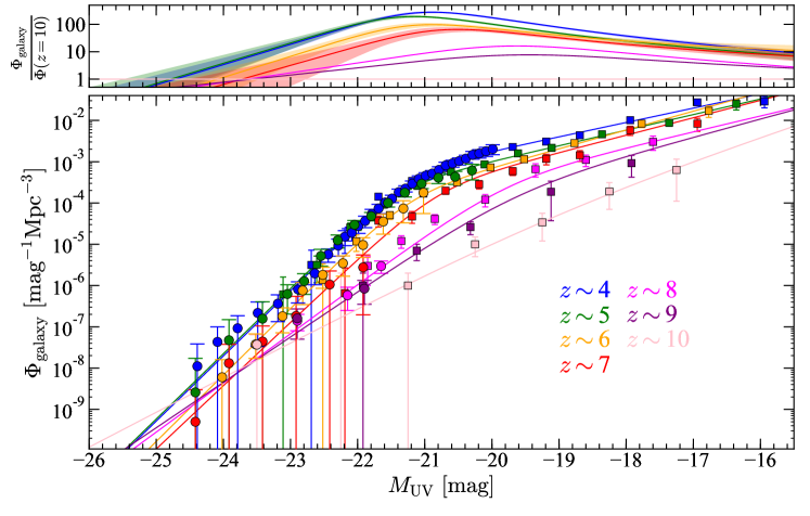
Figure 11.— Evolution of the rest-frame UV luminosity functions of galaxies from $z\sim 10$ to $z\sim 4$. The bottom panel shows the luminosity functions at $z\sim 4-10$, and the blue, green, orange, red, magenta, purple, and pink symbols show results at $z\sim 4$, $5$, $6$, $7$, $8$, $9$, and $10$, respectively. The circles at $z\sim 4-7$ show our results based on the HSC-SSP survey data, and those at $z\sim 8-10$ are taken from Bowler et al. (2020). The squares show results for galaxies in Bouwens et al. (2021). The lines show the best-fit DPL functions in this study at $z\sim 4-7$ and Bowler et al. (2020) at $z\sim 8-10$. The top panel shows ratios of the number densities relative to those at $z\sim 10$. The shaded regions at $z\sim 4-7$ correspond to the $2\sigma$ uncertainties of the luminosity function parameters. The number density of typical galaxies ($M_{\mathrm{UV}}=M^{*}_{\mathrm{UV}}\sim-21$ mag) significantly increases by a factor of $\sim 100$ from $\sim 10$ to $4$, while that of faint galaxies ($M_{\mathrm{UV}}\sim-16$ mag) mildly increases by a factor of $\sim 10$. The number density of the bright galaxies at $-25\lesssim M_{\mathrm{UV}}\lesssim-23$ mag does not significantly change at $z\sim 4-10$.

In Figure 10, we show the best-fit functions of these three functional forms with the obtained galaxy UV luminosity function results. Table 7 summarizes the best-fit parameters and the reduced $\chi^{2}$ values. We find that the DPL and the lensed Schechter functions provide better fits to the observed galaxy UV luminosity functions than the original Schechter functions. The bright-end shapes of the observed galaxy UV luminosity functions cannot be explained by the Schechter functions. The significances of the bright end excess of the number density beyond the Schechter functions are $2.9\sigma$, $1.9\sigma$, $2.8\sigma$, and $2.0\sigma$ at $z\sim 4$, $5$, $6$, and $7$, respectively. Note that the significances are lower than those in Ono et al. (2018) at $z\sim 4$ and $7$ because this time we consider the uncertainties of the spectroscopic galaxy fractions, which are not taken into account in Ono et al. (2018). The physical origin of this bright end excess of the number density beyond the Schechter function will be discussed in Section 6.3. The DPL function provides a better fit to the data points than the lensed Schechter function at $z\sim 4-6$, although the significance of this difference is low. The significances of the excess beyond the lensed Schechter functions are $2.5(2.7)\sigma$, $1.4(1.6)\sigma$, $2.1(2.4)\sigma$, and $1.4(1.6)\sigma$ at $z\sim 4$, $5$, $6$, and $7$, respectively, for the optical depth of Barone-Nugent et al. (2015) (Takahashi et al. 2011), slightly smaller than those beyond the Schechter functions.

4.2.3 Redshift Evolution

Figure 11 shows our galaxy luminosity functions at $z\sim 4-7$ with those of Bouwens et al. (2021) at $z\sim 4-10$ and of Bowler et al. (2020) at $z\sim 8-10$. Although Bowler et al. (2020) do not subtract AGN contributions from their estimated luminosity functions, the number densities of their bright sources at $z\sim 8-10$ are likely dominated by galaxies, not by quasars, given the rapid decrease of the quasar luminosity function from $z\sim 3$ to $6$ as discussed in Section 4.1.4. Figure 11 suggests that the number density of typical galaxies ($M_{\mathrm{UV}}=M^{*}_{\mathrm{UV}}\sim-21$ mag) significantly increases by a factor of $\sim 100$ from $\sim 10$ to $4$, while that of faint galaxies ($M_{\mathrm{UV}}\sim-16$ mag) mildly increases by a factor of $\sim 10$. Our comparison also shows that the number density of the bright galaxies at $-25\lesssim M_{\mathrm{UV}}\lesssim-23$ mag does not significantly change at $z\sim 4-10$, and is consistent with no evolution within the $2\sigma$ errors. This is consistent with Bowler et al. (2021), who report little evolution of the number density of bright galaxies at $z\gtrsim 5$, although in their comparison they do not subtract AGN contributions from luminosity functions at $z\sim 5-7$. This agreement is expected because Bowler et al. (2021) compare the number densities of $M_{\mathrm{UV}}>-24$ mag sources that are not dominated by AGNs. As shown in Section 4.1.4, the number density of $M_{\mathrm{UV}}\lesssim-24$ mag sources is dominated by AGNs and evolves rapidly, and we need to subtract AGN contributions to fairly compare the galaxy luminosity functions at the bright end.

5. Clustering Analysis

5.1. Angular Correlation Function

We calculate angular correlation functions to evaluate the clustering strength of galaxies at $z\sim 2-6$. We use the galaxy samples at $z\sim 1.7$, $2.2$, $3$, $4$, $5$, and $6$ constructed in Sections 3.1 and 3.5. Note that we do not remove AGNs from our source catalogs. To test the dependence of the clustering strength on the luminosity, we divide our galaxy samples into subsamples by UV magnitude thresholds ($m_{\mathrm{UV}}^{\mathrm{th}}$). The number of dropouts in the subsamples and their magnitude thresholds are summarized in Table 8. We do not use sources brighter than $m_{\mathrm{UV}}^{\mathrm{cut}}=20.0$ mag at each redshift in our analysis. Changing this cut to a fainter magnitude (e.g., 23.0 mag) to remove AGNs does not change results of the angular correlation functions within the errors, because the number of such bright sources is small (see Harikane et al. 2018a). Note that in the calculations we do not use sources in some part of the fields in the Wide layer whose depths are shallow.

We calculate observed angular correlation functions of the subsamples, $\omega_{\mathrm{obs}}(\theta)$, using an estimator proposed by Landy & Szalay (1993),

$$\omega_{\mathrm{obs}}(\theta)=\frac{DD(\theta)-2DR(\theta)+RR(\theta)}{RR(\theta)},$$ (41)

where $DD(\theta)$, $DR(\theta)$, and $RR(\theta)$ are the numbers of galaxy-galaxy, galaxy-random, and random-random pairs normalized by the total numbers of pairs. We use the random catalog whose surface number density is $100\ \mathrm{arcmin^{-2}}$ with the same geometrical shape as the observational data including the mask positions (Coupon et al. 2018). Corrections for contaminations (e.g., Equation (29) in Harikane et al. (2016)) are not applied because the clustering strength of the interlopers is not well-measured. We calculate angular correlation functions in individual fields, and obtain the best-estimate that is the mean weighted by the effective area in each field. Figures 12 and 13 show our calculated angular correlation functions of the subsamples at $z\sim 2-3$ and $4-6$, respectively. We compare our obtained correlation functions with the literature in Figure 14. Our correlations functions are in good agreement with those of Adelberger et al. (2005), Savoy et al. (2011), and Hildebrandt et al. (2009).

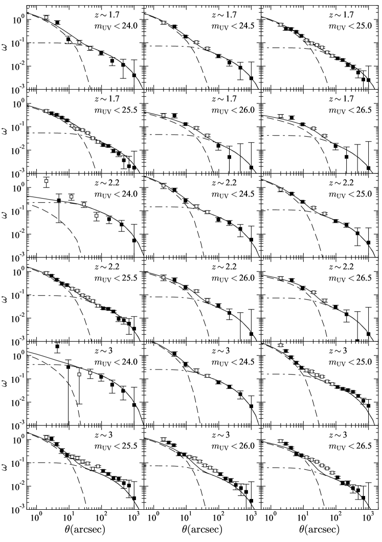
Figure 12.— Obtained angular correlation functions of the subsamples and their best-fit by the HOD models at $z\sim 1.7$, $2.2$, and $3$. The black squares denote the angular correlation function of the subsample at each redshift. The data denoted by the open squares are not used in our HOD model fitting because they are at too-small scales or possibly affected by the non-linear halo bias effect. The dashed and dot-dashed lines represent the one-halo and two-halo terms, respectively, and the solid line is the summations of the one-halo and two-halo terms.

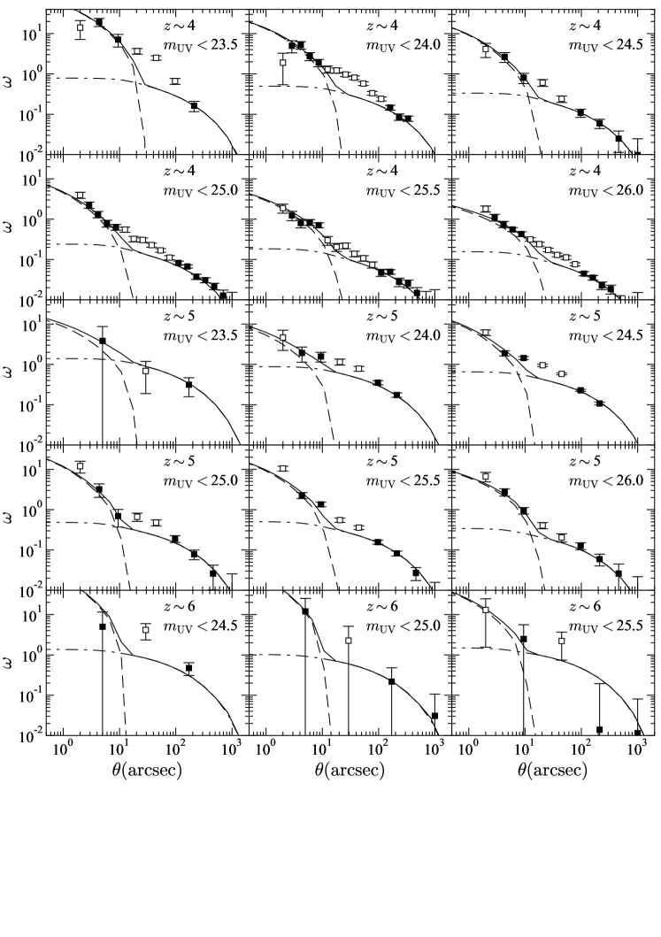
Figure 13.— Same as Figure 12 but at $z\sim 4$, $5$, and $6$.

Table 8Summary of the Clustering Measurements with the HOD Model.

$\bar{z}$	$m_{\mathrm{UV}}^{\mathrm{th}}$	$N$	$n_{\mathrm{obs}}$	$M_{\mathrm{UV}}^{\mathrm{th}}$	$SFR$	$\mathrm{log}M_{\mathrm{min}}$	$\mathrm{log}M_{\mathrm{sat}}$	$\mathrm{log}\left<M_{\mathrm{h}}\right>$	$b_{\mathrm{g}}^{\mathrm{eff}}$	$\mathrm{log}f_{\mathrm{sat}}$	$\chi^{2}/\mathrm{dof}$
(1)	(2)	(3)	(4)	(5)	(6)	(7)	(8)	(9)	(10)	(11)	(12)
$z\sim 1.7$
$1.7$	$24.0$	$16219$	$3.6\times 10^{-4}$	$-20.5$	$31.0$	$12.46^{+0.03}_{-0.03}$	$14.18^{+0.19}_{-0.09}$	$12.82^{+0.02}_{-0.02}$	$2.42^{+0.03}_{-0.05}$	$-1.45^{+0.08}_{-0.17}$	$9.1/5$
$1.7$	$24.5$	$42719$	$1.1\times 10^{-3}$	$-20.0$	$16.3$	$12.09^{+0.03}_{-0.04}$	$13.47^{+0.09}_{-0.09}$	$12.61^{+0.01}_{-0.02}$	$2.04^{+0.03}_{-0.02}$	$-1.14^{+0.05}_{-0.08}$	$2.4/5$
$1.7$	$25.0$	$87813$	$2.4\times 10^{-3}$	$-19.5$	$8.6$	$11.79^{+0.03}_{-0.04}$	$12.86^{+0.10}_{-0.06}$	$12.56^{+0.01}_{-0.02}$	$1.86^{+0.01}_{-0.02}$	$-0.93^{+0.03}_{-0.05}$	$4.1/10$
$1.7$	$25.5$	$150962$	$4.5\times 10^{-3}$	$-19.0$	$4.5$	$11.55^{+0.04}_{-0.03}$	$12.48^{+0.06}_{-0.06}$	$12.55^{+0.02}_{-0.01}$	$1.76^{+0.01}_{-0.02}$	$-0.88^{+0.02}_{-0.03}$	$4.9/10$
$1.7$	$26.0$	$24950$	$7.3\times 10^{-3}$	$-18.5$	$2.4$	$11.33^{+0.04}_{-0.04}$	$12.28^{+0.06}_{-0.07}$	$12.49^{+0.02}_{-0.02}$	$1.62^{+0.03}_{-0.02}$	$-0.95^{+0.03}_{-0.03}$	$2.5/3$
$1.7$	$26.5$	$36015$	$1.1\times 10^{-2}$	$-18.0$	$1.2$	$11.16^{+0.05}_{-0.04}$	$12.08^{+0.08}_{-0.07}$	$12.46^{+0.02}_{-0.03}$	$1.54^{+0.02}_{-0.03}$	$-0.99^{+0.02}_{-0.06}$	$2.9/3$
$z\sim 2.2$
$2.2$	$24.0$	$4927$	$8.4\times 10^{-5}$	$-21.0$	$59.1$	$12.72^{+0.03}_{-0.02}$	$(15.91)$	$12.91^{+0.02}_{-0.01}$	$3.62^{+0.07}_{-0.05}$	$-3.03^{+0.06}_{-0.06}$	$1.1/4$
$2.2$	$24.5$	$14185$	$3.6\times 10^{-4}$	$-20.5$	$31.0$	$12.30^{+0.03}_{-0.03}$	$13.92^{+0.11}_{-0.11}$	$12.61^{+0.02}_{-0.02}$	$2.86^{+0.04}_{-0.05}$	$-1.43^{+0.08}_{-0.10}$	$3.3/5$
$2.2$	$25.0$	$32241$	$1.1\times 10^{-3}$	$-20.0$	$16.3$	$11.95^{+0.04}_{-0.02}$	$13.23^{+0.12}_{-0.08}$	$12.41^{+0.01}_{-0.02}$	$2.42^{+0.03}_{-0.03}$	$-1.20^{+0.06}_{-0.07}$	$0.8/5$
$2.2$	$25.5$	$59623$	$2.4\times 10^{-3}$	$-19.5$	$8.6$	$11.68^{+0.04}_{-0.03}$	$12.62^{+0.11}_{-0.05}$	$12.34^{+0.01}_{-0.02}$	$2.21^{+0.03}_{-0.02}$	$-1.02^{+0.02}_{-0.05}$	$9.8/10$
$2.2$	$26.0$	$9196$	$4.5\times 10^{-3}$	$-19.0$	$4.5$	$11.45^{+0.02}_{-0.05}$	$12.23^{+0.15}_{-0.11}$	$12.32^{+0.04}_{-0.09}$	$2.06^{+0.04}_{-0.08}$	$-0.98^{+0.08}_{-0.14}$	$1.4/3$
$2.2$	$26.5$	$13949$	$7.3\times 10^{-3}$	$-18.5$	$2.4$	$11.26^{+0.06}_{-0.02}$	$11.94^{+0.09}_{-0.05}$	$12.32^{+0.02}_{-0.04}$	$1.97^{+0.04}_{-0.04}$	$-0.96^{+0.03}_{-0.05}$	$3.4/3$
$z\sim 3$
$2.9$	$24.0$	$4607$	$5.7\times 10^{-5}$	$-21.5$	$114.1$	$12.55^{+0.02}_{-0.02}$	$(15.39)$	$12.68^{+0.02}_{-0.01}$	$4.66^{+0.09}_{-0.04}$	$-2.75^{+0.02}_{-0.08}$	$3.0/6$
$2.9$	$24.5$	$18013$	$2.5\times 10^{-4}$	$-21.0$	$59.9$	$12.19^{+0.02}_{-0.03}$	$13.80^{+0.19}_{-0.11}$	$12.42^{+0.01}_{-0.02}$	$3.71^{+0.05}_{-0.05}$	$-1.57^{+0.10}_{-0.15}$	$1.1/5$
$2.9$	$25.0$	$57199$	$6.7\times 10^{-4}$	$-20.5$	$31.5$	$11.92^{+0.03}_{-0.02}$	$13.12^{+0.12}_{-0.07}$	$12.26^{+0.01}_{-0.02}$	$3.23^{+0.04}_{-0.03}$	$-1.30^{+0.04}_{-0.06}$	$9.7/10$
$2.9$	$25.5$	$11257$	$1.5\times 10^{-3}$	$-20.0$	$16.5$	$11.71^{+0.04}_{-0.02}$	$12.55^{+0.14}_{-0.04}$	$12.21^{+0.01}_{-0.02}$	$2.90^{+0.04}_{-0.03}$	$-1.11^{+0.05}_{-0.06}$	$10.5/10$
$2.9$	$26.0$	$23231$	$2.6\times 10^{-3}$	$-19.5$	$8.7$	$11.55^{+0.03}_{-0.04}$	$12.20^{+0.06}_{-0.07}$	$12.20^{+0.01}_{-0.02}$	$2.72^{+0.02}_{-0.05}$	$-1.03^{+0.03}_{-0.03}$	$15.4/10$
$2.9$	$26.5$	$43111$	$4.4\times 10^{-3}$	$-19.0$	$4.6$	$11.36^{+0.05}_{-0.03}$	$11.84^{+0.10}_{-0.04}$	$12.21^{+0.02}_{-0.01}$	$2.55^{+0.04}_{-0.04}$	$-0.97^{+0.02}_{-0.03}$	$15.7/10$
$z\sim 4$
$3.8$	$23.5$	$4971$	$1.1\times 10^{-6}$	$-22.5$	$186.0$	$13.08^{+0.03}_{-0.01}$	$15.25^{+0.12}_{-0.09}$	$13.01^{+0.01}_{-0.01}$	$8.55^{+0.08}_{-0.09}$	$-2.25^{+0.09}_{-0.11}$	$0.4/2$
$3.8$	$24.0$	$19125$	$1.0\times 10^{-5}$	$-22.0$	$106.1$	$12.71^{+0.02}_{-0.02}$	$14.80^{+0.09}_{-0.08}$	$12.73^{+0.01}_{-0.02}$	$6.70^{+0.05}_{-0.09}$	$-2.12^{+0.07}_{-0.07}$	$4.9/6$
$3.8$	$24.5$	$8059$	$6.1\times 10^{-5}$	$-21.5$	$60.5$	$12.32^{+0.03}_{-0.02}$	$13.96^{+0.34}_{-0.09}$	$12.43^{+0.01}_{-0.02}$	$5.35^{+0.07}_{-0.07}$	$-1.68^{+0.08}_{-0.31}$	$0.2/5$
$3.8$	$25.0$	$27735$	$2.6\times 10^{-4}$	$-21.0$	$34.5$	$11.98^{+0.03}_{-0.02}$	$13.23^{+0.13}_{-0.08}$	$12.18^{+0.02}_{-0.01}$	$4.41^{+0.06}_{-0.06}$	$-1.50^{+0.05}_{-0.10}$	$8.2/10$
$3.8$	$25.5$	$8059$	$8.1\times 10^{-4}$	$-20.5$	$19.7$	$11.66^{+0.02}_{-0.03}$	$12.24^{+0.07}_{-0.10}$	$12.02^{+0.01}_{-0.02}$	$3.85^{+0.04}_{-0.05}$	$-1.23^{+0.05}_{-0.04}$	$14.1/10$
$3.8$	$26.0$	$16494$	$1.6\times 10^{-3}$	$-20.0$	$11.2$	$11.48^{+0.04}_{-0.02}$	$11.94^{+0.10}_{-0.04}$	$11.94^{+0.02}_{-0.01}$	$3.44^{+0.05}_{-0.04}$	$-1.27^{+0.03}_{-0.05}$	$1.4/10$
$z\sim 5$
$4.9$	$23.5$	$1650$	$2.2\times 10^{-7}$	$-22.9$	$325.1$	$12.95^{+0.02}_{-0.01}$	$16.65^{+1.57}_{-0.12}$	$12.81^{+0.01}_{-0.01}$	$11.02^{+0.08}_{-0.12}$	$-3.86^{+0.12}_{-1.57}$	$0.1/1$
$4.9$	$24.0$	$21453$	$2.9\times 10^{-6}$	$-22.4$	$180.4$	$12.60^{+0.01}_{-0.02}$	$15.70^{+0.82}_{-0.07}$	$12.55^{+0.01}_{-0.01}$	$8.64^{+0.08}_{-0.10}$	$-3.21^{+0.14}_{-0.69}$	$2.6/3$
$4.9$	$24.5$	$63308$	$1.7\times 10^{-5}$	$-21.9$	$100.1$	$12.29^{+0.03}_{-0.00}$	$14.63^{+0.11}_{-0.06}$	$12.32^{+0.02}_{-0.01}$	$7.11^{+0.10}_{-0.06}$	$-2.49^{+0.06}_{-0.08}$	$27.2/3$
$4.9$	$25.0$	$5305$	$6.4\times 10^{-5}$	$-21.4$	$55.6$	$12.00^{+0.02}_{-0.01}$	$13.45^{+0.46}_{-0.08}$	$12.09^{+0.01}_{-0.02}$	$6.17^{+0.06}_{-0.08}$	$-1.89^{+0.09}_{-0.40}$	$1.7/5$
$4.9$	$25.5$	$13688$	$1.9\times 10^{-4}$	$-20.9$	$30.8$	$11.76^{+0.02}_{-0.02}$	$12.57^{+0.13}_{-0.09}$	$11.93^{+0.02}_{-0.01}$	$5.37^{+0.06}_{-0.06}$	$-1.62^{+0.06}_{-0.07}$	$9.7/5$
$4.9$	$26.0$	$3349$	$4.2\times 10^{-4}$	$-20.4$	$17.1$	$11.57^{+0.03}_{-0.02}$	$11.86^{+0.11}_{-0.06}$	$11.83^{+0.01}_{-0.02}$	$4.99^{+0.07}_{-0.06}$	$-1.44^{+0.04}_{-0.07}$	$1.4/5$
$z\sim 6$
$5.9$	$24.5$	$2026$	$1.6\times 10^{-6}$	$-22.2$	$163.3$	$12.33^{+0.02}_{-0.02}$	$(14.67)$	$12.24^{+0.01}_{-0.01}$	$10.09^{+0.09}_{-0.09}$	$-2.63^{+0.03}_{-0.02}$	$2.9/2$
$5.9$	$25.0$	$328$	$7.7\times 10^{-6}$	$-21.7$	$85.8$	$12.09^{+0.01}_{-0.02}$	$13.73^{+5.67}_{-0.28}$	$12.07^{+0.01}_{-0.02}$	$8.77^{+0.04}_{-0.14}$	$-2.19^{+0.40}_{-4.01}$	$1.0/2$
$5.9$	$25.5$	$480$	$3.2\times 10^{-5}$	$-21.2$	$45.1$	$11.78^{+0.02}_{-0.02}$	$(12.93)$	$11.81^{+0.02}_{-0.01}$	$7.68^{+0.05}_{-0.11}$	$-2.41^{+0.01}_{-0.00}$	$1.9/3$

Note. — (1) Mean redshift. (2) Threshold apparent magnitude in the rest-frame UV band. (3) Number of galaxies in the subsample. (4) Number density of galaxies in the subsample in units of $\mathrm{Mpc^{-3}}$. (5) Threshold absolute magnitude in the rest-frame UV band. (6) SFR corresponding to $M_{\mathrm{UV}}^{\mathrm{th}}$ after the extinction correction in units of $M_{\odot}\ \mathrm{yr^{-1}}$. (7) Best-fit value of $M_{\mathrm{min}}$ in units of $M_{\odot}$. (8) Best-fit value of $M_{\mathrm{sat}}$ in units of $M_{\odot}$. The value in parenthesis is derived from $M_{\mathrm{min}}$ via Equation (53). (9) Mean halo mass in units of $M_{\odot}$. (10) Effective bias. (11) Satellite fraction. (12) Reduced $\chi^{2}$ value.

Due to the finite size of our survey fields, the observed correlation functions is underestimated by a constant value known as the integral constraint, $IC$ (Groth & Peebles 1977). Including a correction for the number of objects in the sample, $N$ (Peebles 1980), the true angular correlation function is given by

$$\omega(\theta)=\omega_{\mathrm{obs}}(\theta)+IC+\frac{1}{N}.$$ (42)

We estimate the integral constraint with

$$IC=\frac{\Sigma_{i}RR(\theta_{i})\omega_{\mathrm{model}}(\theta_{i})}{\Sigma_{i}RR(\theta_{i})},$$ (43)

where $\omega_{\mathrm{model}}(\theta)$ is the best-fit model of the correlation function, and $i$ refers the angular bin. $IC$ and $\omega_{\mathrm{model}}(\theta)$ are simultaneously determined in the model fitting in Section 5.2.

We estimate statistical errors of the angular correlation functions using the Jackknife estimator. We divide each subsample into Jackknife samples of about $1000^{2}\ \mathrm{arcsec}^{2}$, whose size is larger than the largest angular scale in the correlation function. Removing one Jackknife sample at a time for each realization, we compute the covariance matrix as

$$C_{ij}=\frac{N_{\mathrm{Jack}}-1}{N_{\mathrm{Jack}}}\sum^{N_{\mathrm{Jack}}}_{l=1}\left[\omega^{l}(\theta_{i})-\bar{\omega}(\theta_{i})\right]\left[\omega^{l}(\theta_{j})-\bar{\omega}(\theta_{j})\right].$$ (44)

where $N_{\mathrm{Jack}}$ is the total number of the Jackknife samples, $\omega^{l}$ is the estimated correlation function from the $l$th realization, and $\bar{\omega}$ is the mean correlation function. We apply a correction factor given by Hartlap et al. (2007) to an inverse covariance matrix in order to compensate for the bias introduced by the noise. The inverse of the square root of the inverse covariance matrix is plotted in Figures 12, 13, 14 as uncertainties.

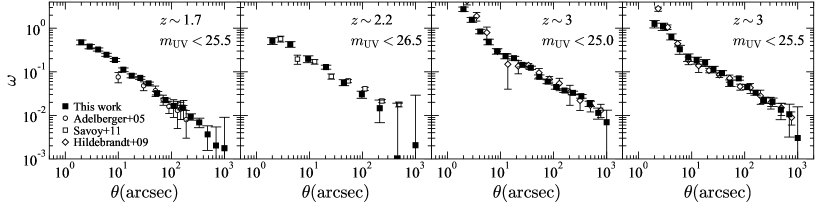
Figure 14.— Comparisons of the angular correlation functions with the literature. The black squares represent the correlation functions in this study. The open circles, squares, and diamonds denote results in Adelberger et al. (2005), Savoy et al. (2011), and Hildebrandt et al. (2009), respectively. Our obtained measurements agree well with these previous studies.

5.2. Halo Occupation Distribution (HOD) Model Fitting

We use an HOD model to investigate the relationship between galaxies and their dark matter halos. The HOD model is an analytic framework quantifying a probability distribution of the number of galaxies in dark matter halos (e.g., Seljak 2000; Peacock & Smith 2000; Ma & Fry 2000). The key assumption in the HOD model is that the probability depends only on the halo mass, $M_{\mathrm{h}}$. We can analytically calculate correlation functions and number densities from the HOD model. Details of the calculations are presented in Harikane et al. (2016).

We fit our HOD model to the observed angular correlation functions and number densities. In the fitting procedures, the best-fit parameters are determined by minimizing the $\chi^{2}$ value,

$$\chi^{2}= \sum_{i,j} \left[\omega(\theta_{i})-\omega_{\mathrm{model}}(\theta_{i})\right]C^{-1}_{i,j}\left[\omega(\theta_{j})-\omega_{\mathrm{model}}(\theta_{j})\right]$$ (45)

$$+ \frac{\left[\mathrm{log}\,n_{\mathrm{g}}^{\mathrm{obs}}-\mathrm{log}\,n_{\mathrm{g}}^{\mathrm{model}}\right]^{2}}{\sigma^{2}_{\mathrm{log}n_{\mathrm{g}}}},$$

where $C^{-1}_{i,j}$ is the inverse covariance matrix, $n_{\mathrm{g}}$ is a space number density of galaxies in the subsample, and $\sigma_{\mathrm{log}n_{\mathrm{g}}}$ is its error. We calculate the number density of galaxies corrected for incompleteness using the galaxy UV luminosity functions derived in this work (Section 4.2) and Bouwens et al. (2021). The galaxy number density of each subsample is presented in Table 8. We assume $10\%$ fractional uncertainties in the number densities as Zheng et al. (2007). This $10\%$ uncertainty is a conservative assumption, because the actual statistical uncertainty is typically less than $5\%$. We constrain the parameters of our HOD model using the Markov Chain Monte Carlo (MCMC) parameter estimation technique.

In our HOD model, an occupation function for central galaxies follows a step function with a smooth transition,

$$\left<N_{\mathrm{cen}}(M_{\mathrm{h}})\right>=\frac{1}{2}\left[1+\mathrm{erf}\left(\frac{\mathrm{log}M_{\mathrm{h}}-\mathrm{log}M_{\mathrm{min}}}{\sqrt{2}\sigma_{\mathrm{log}M_{\mathrm{h}}}}\right)\right].$$ (46)

An occupation function for satellite galaxies is expressed by a power law with a mass cut,

$$\left<N_{\mathrm{sat}}(M_{\mathrm{h}})\right>=\left<N_{\mathrm{cen}}(M_{\mathrm{h}})\right>\left(\frac{M_{\mathrm{h}}-M_{\mathrm{cut}}}{M_{\mathrm{sat}}}\right)^{\alpha}.$$ (47)

The total occupation function is

$$\left<N_{\mathrm{tot}}(M_{\mathrm{h}})\right>=\left<N_{\mathrm{cen}}(M_{\mathrm{h}})\right>+\left<N_{\mathrm{sat}}(M_{\mathrm{h}})\right>.$$ (48)

These functional forms are motivated by N-body simulations, smoothed particle hydrodynamic simulations, and semi-analytic models for both low and high redshift galaxies (e.g., Kravtsov et al. 2004; Zheng et al. 2005; Garel et al. 2015). Indeed, previous studies demonstrate that this HOD model can explain observed angular correlation functions of high redshift galaxies (Harikane et al. 2016, 2018a; Ishikawa et al. 2017).

We calculate the mean dark matter halo mass of galaxies including both the central and satellite galaxies, $\left<M_{\mathrm{h}}\right>$, effective galaxy bias, $b_{\mathrm{g}}^{\mathrm{eff}}$, and the satellite fraction, $f_{\mathrm{sat}}$, as follows:

$$\left<M_{\mathrm{h}}\right> = \frac{1}{n_{\mathrm{g}}}\int dM_{\mathrm{h}}\frac{dn}{dM_{\mathrm{h}}}(M_{\mathrm{h}},z)N_{\mathrm{tot}}(M_{\mathrm{h}})M_{\mathrm{h}},$$ (49)

$$b_{\mathrm{g}}^{\mathrm{eff}} = \frac{1}{n_{\mathrm{g}}}\int dM_{\mathrm{h}}\frac{dn}{dM_{\mathrm{h}}}(M_{\mathrm{h}},z)N_{\mathrm{tot}}(M_{\mathrm{h}})b_{\mathrm{h}}(M_{\mathrm{h}},z),$$ (50)

$$f_{\mathrm{sat}} = \frac{1}{n_{\mathrm{g}}}\int dM_{\mathrm{h}}\frac{dn}{dM_{\mathrm{h}}}(M_{\mathrm{h}},z)N_{\mathrm{sat}}(M_{\mathrm{h}}),$$ (51)

where $\frac{dn}{dM_{\mathrm{h}}}(M_{\mathrm{h}},z)$, $b_{\mathrm{h}}(M_{\mathrm{h}},z)$, and $n_{\mathrm{g}}$ are the halo mass function, halo bias, and the galaxy number density in the model (Equation (51) in Harikane et al. 2016), respectively. We use the Behroozi et al. (2013) halo mass function, which is a modification of the Tinker et al. (2008) mass function, and is calibrated at $z>3$, the NFW dark matter halo profile (Navarro et al. 1996, 1997), the Duffy et al. (2008) concentration parameter, and the Smith et al. (2003) non-linear matter power spectrum.

Some theoretical studies claim that the halo bias is scale-dependent in the quasi-linear scale of $r\sim 50\ \mathrm{Mpc}$ (the non-linear halo bias effect; Reed et al. 2009; Jose et al. 2013, 2016, 2017). However, in this study, we assume the scale-independent linear halo bias of Tinker et al. (2010), $b(M_{\mathrm{h}},z)$. Instead, we do not use the angular correlation functions at $10\arcsec<\theta<90\arcsec$ ($10\arcsec<\theta<120\arcsec$) in the UltraDeep and Deep (Wide) layers, because they could be affected by the non-linear halo bias effect. We also do not use the measurements at $\theta\leq 2\arcsec$ that are possibly affected by the source confusion.

The HOD model has five parameters, $M_{\mathrm{min}}$, $\sigma_{\mathrm{log}M_{\mathrm{h}}}$, $M_{\mathrm{cut}}$, $M_{\mathrm{sat}}$, and $\alpha$. We take $M_{\mathrm{min}}$ and $M_{\mathrm{sat}}$ as free parameters, which control typical masses of halos having one central and satellite galaxies, respectively, as previous studies (Harikane et al. 2016, 2018a). We fix $\sigma_{\mathrm{log}M_{\mathrm{h}}}=0.2$ and $\alpha=1.0$, following results of previous studies (e.g., Kravtsov et al. 2004; Zheng et al. 2005; Conroy et al. 2006; Ishikawa et al. 2017). To derive $M_{\mathrm{cut}}$ from $M_{\mathrm{min}}$, we use the relation

$$M_{\mathrm{cut}}=M_{\mathrm{min}}^{-0.5},$$ (52)

which is given by Coupon et al. (2015). Because the exact value of $M_{\mathrm{cut}}$ has very little importance compared to the other parameters, this assumption does not change any of our conclusions. For subsamples whose correlation functions are not accurately determined due to the small number of galaxies (subsamples of $z\sim 2.2$ $m_{\mathrm{UV}}^{\mathrm{th}}=24.0$ mag, $z\sim 3$ $m_{\mathrm{UV}}^{\mathrm{th}}=24.0$ mag, and $z\sim 6$ $m_{\mathrm{UV}}^{\mathrm{th}}=24.5,\ 25.5$), we also use the following relation calibrated with results in Harikane et al. (2018a).

$$\mathrm{log}M_{\mathrm{sat}}=3.16\ \mathrm{log}M_{\mathrm{min}}-24.33.$$ (53)

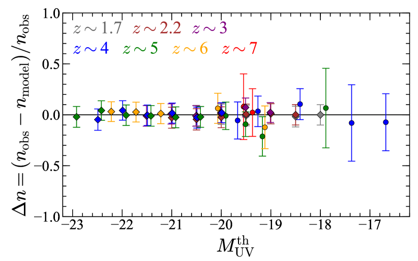
Figure 15.— Comparison of the number densities between the HOD models and observations. The gray, brown, purple, blue, green, orange, and red squares (circles) represent the relative differences of the number densities between the HOD models and observations for the subsamples in this work (in Harikane et al. 2016), at $z\sim 1.7$, $2.2$, $3$, $4$, $5$, $6$, and $7$, respectively, as a function of the threshold absolute UV magnitudes, $M_{\mathrm{UV}}^{\mathrm{th}}$.

We plot the observed angular correlation functions and predictions from their best-fit HOD models in Figures 12 and 13. The best-fit parameters and their $1\sigma$ errors are presented in Table 8. The HOD models can reproduce the observed correlation functions at small ($2\lesssim\theta\lesssim 10\arcsec$) and large ($\theta\gtrsim 100\arcsec$) scales. However, the models underpredict the correlation functions by a factor of $1.5-6$ in $10\arcsec\lesssim\theta\lesssim 100\arcsec$, the transition scale between 1- and 2-halo terms (the quasi-linear scale), especially in the subsamples at $z\gtrsim 3$. These results indicate that the correlation functions at $10\arcsec\lesssim\theta\lesssim 100\arcsec$ can not be explained by the scale-independent halo bias due to the non-linear halo bias effect in this quasi-linear scale (Jose et al. 2013, 2016, 2017). We also find that the best-fit HOD models slightly underpredict the correlation functions of the subsamples of $z\sim 3$ and $m_{\mathrm{UV}}<25.5$ and $26.0$ at $\theta\geq 100\arcsec$, although the reduced $\chi^{2}$ values are not bad ($\chi^{2}/\mathrm{dof}=1.05,1.54$). We have tried to fit the correlation functions of these subsamples with taking $M_{\mathrm{min}}$, $\sigma_{\mathrm{log}M_{\mathrm{h}}}$, $M_{\mathrm{sat}}$, and $\alpha$ as free parameters, but the results does not significantly change. In Figure 15, we compare the observed number densities and predictions from the best-fit HOD models, showing good agreement.

5.3. $M_{\mathrm{UV}}-M_{\mathrm{h}}$ Relation

Figure 16 shows our results of the halo mass, $M_{\mathrm{h}}$, at $z\sim 2-6$ as a function of the UV magnitude, $M_{\mathrm{UV}}$, with previous studies (Harikane et al. 2016, 2018a) at $z\sim 4-7$. We plot $M_{\mathrm{min}}$ and $M_{\mathrm{UV}}^{\mathrm{th}}$ as $M_{\mathrm{h}}$ and $M_{\mathrm{UV}}$, respectively. Table 9 summarizes the results of this work at $z\sim 2-6$ and of Harikane et al. (2016). We find that the new results obtained in this work are consistent with our previous measurements in Harikane et al. (2018a), which are indicated by the crosses in Figure 16. The halo mass of $z\sim 4-6$ galaxies identified in the HSC data ranges from $3\times 10^{11}\ M_{\odot}$ to $1\times 10^{13}\ M_{\odot}$, which is more massive than those of galaxies identified in the Hubble data (Harikane et al. 2016). The combination of the Hubble and HSC data allows us to investigate the $M_{\mathrm{UV}}-M_{\mathrm{h}}$ relation over two orders of magnitude in the halo mass at $z\sim 4$ and $5$. Thus in the following discussion, we will mainly use the results of this work and of Harikane et al. (2016). There is a positive correlation between the UV luminosities and the halo masses at all redshifts, indicating that more UV-luminous galaxies reside in more massive halos, as suggested by previous studies. The slope of the $M_{\mathrm{UV}}-M_{\mathrm{h}}$ relation becomes steeper at the brighter magnitude, which is similar to the local $M_{\mathrm{*}}-M_{\mathrm{h}}$ relation (e.g., Leauthaud et al. 2012; Behroozi et al. 2013, 2019; Moster et al. 2013, 2018; Coupon et al. 2015). Note that the uncertainty of the halo mass at $z\sim 6$ is as small as those at $z\sim 4-5$ albeit with the large errors in the correlation function measurement at $z\sim 6$, because the halo mass is mainly determined by the number density whose uncertainty is $10\%$, and the slope of the halo mass function is very steep at high redshift.

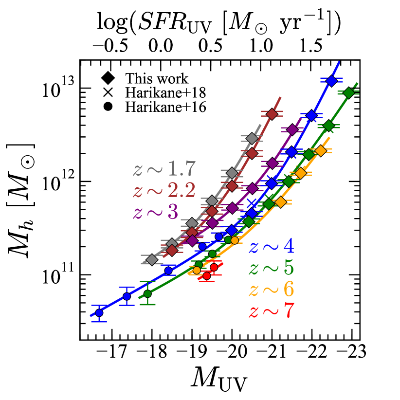
Figure 16.— $M_{\mathrm{UV}}-M_{\mathrm{h}}$ relation. The gray, brown, purple, blue, green, orange, and red filled diamonds (circles) denote the halo masses as a function of the UV magnitude at $z\sim 1.7$, $2.2$, $3$, $4$, $5$, $6$, and $7$, respectively, for the subsamples in this work (in Harikane et al. 2016). We plot $M_{\mathrm{min}}$ and $M_{\mathrm{UV}}^{\mathrm{th}}$ as $M_{\mathrm{h}}$ and $M_{\mathrm{UV}}$, respectively. The crosses are results of the previous work based on the early HSC-SSP data (Harikane et al. 2018b). The solid curves show the best-fit relations of Equation (54).

Table 9Halo mass and $SFR/\dot{M}_{\mathrm{h}}$ in This Study.

$\bar{z}$	$M_{\mathrm{UV}}^{\mathrm{th}}$	$SFR$	$\mathrm{log}M_{\mathrm{h}}$	$SFR/\dot{M}_{\mathrm{h}}\ (10^{-2})$
(1)	(2)	(3)	(4)	(5)
1.7	-20.5	$31.0$	$12.46_{-0.03}^{+0.03}$	$3.12_{-0.26}^{+0.23}$
1.7	-20.0	$16.3$	$12.09_{-0.04}^{+0.03}$	$4.43_{-0.36}^{+0.44}$
1.7	-19.5	$8.6$	$11.79_{-0.04}^{+0.03}$	$5.20_{-0.44}^{+0.51}$
1.7	-19.0	$4.5$	$11.55_{-0.03}^{+0.04}$	$5.19_{-0.57}^{+0.40}$
1.7	-18.5	$2.4$	$11.33_{-0.04}^{+0.04}$	$4.91_{-0.53}^{+0.52}$
1.7	-18.0	$1.2$	$11.16_{-0.04}^{+0.05}$	$4.06_{-0.56}^{+0.42}$
2.2	-21.0	$59.1$	$12.72_{-0.02}^{+0.03}$	$1.91_{-0.16}^{+0.10}$
2.2	-20.5	$31.0$	$12.30_{-0.03}^{+0.03}$	$3.04_{-0.24}^{+0.23}$
2.2	-20.0	$16.3$	$11.95_{-0.02}^{+0.04}$	$4.02_{-0.45}^{+0.21}$
2.2	-19.5	$8.6$	$11.68_{-0.03}^{+0.04}$	$4.31_{-0.49}^{+0.32}$
2.2	-19.0	$4.5$	$11.45_{-0.05}^{+0.02}$	$4.15_{-0.25}^{+0.52}$
2.2	-18.5	$2.4$	$11.26_{-0.02}^{+0.06}$	$3.59_{-0.60}^{+0.19}$
2.9	-21.5	$114.1$	$12.55_{-0.02}^{+0.02}$	$3.45_{-0.18}^{+0.18}$
2.9	-21.0	$59.9$	$12.19_{-0.03}^{+0.02}$	$4.59_{-0.24}^{+0.35}$
2.9	-20.5	$31.5$	$11.92_{-0.02}^{+0.03}$	$4.85_{-0.40}^{+0.25}$
2.9	-20.0	$16.5$	$11.71_{-0.02}^{+0.04}$	$4.39_{-0.47}^{+0.23}$
2.9	-19.5	$8.7$	$11.55_{-0.04}^{+0.03}$	$3.49_{-0.27}^{+0.34}$
2.9	-19.0	$4.6$	$11.36_{-0.03}^{+0.05}$	$3.00_{-0.42}^{+0.22}$
3.8	-22.5	$186.0$	$13.08_{-0.01}^{+0.03}$	$0.90_{-0.07}^{+0.02}$
3.8	-22.0	$106.1$	$12.71_{-0.02}^{+0.02}$	$1.31_{-0.07}^{+0.06}$
3.8	-21.5	$60.5$	$12.32_{-0.02}^{+0.03}$	$2.00_{-0.16}^{+0.10}$
3.8	-21.0	$34.5$	$11.98_{-0.02}^{+0.03}$	$2.71_{-0.22}^{+0.14}$
3.8	-20.5	$19.7$	$11.66_{-0.03}^{+0.02}$	$3.49_{-0.19}^{+0.26}$
3.8	-20.0	$11.2$	$11.48_{-0.02}^{+0.04}$	$3.14_{-0.34}^{+0.16}$
3.8	-19.7	$7.8$	$11.41_{-0.05}^{+0.04}$	$2.34_{-0.25}^{+0.28}$
3.8	-19.3	$5.0$	$11.30_{-0.05}^{+0.04}$	$1.93_{-0.21}^{+0.23}$
3.8	-18.4	$1.9$	$11.04_{-0.05}^{+0.06}$	$1.44_{-0.24}^{+0.17}$
3.8	-17.4	$0.6$	$10.77_{-0.10}^{+0.10}$	$0.91_{-0.26}^{+0.20}$
3.8	-16.7	$0.3$	$10.59_{-0.10}^{+0.08}$	$0.66_{-0.15}^{+0.14}$
4.9	-22.9	$325.1$	$12.95_{-0.01}^{+0.02}$	$1.36_{-0.07}^{+0.03}$
4.9	-22.4	$180.4$	$12.60_{-0.02}^{+0.01}$	$1.80_{-0.05}^{+0.09}$
4.9	-21.9	$100.1$	$12.29_{-0.00}^{+0.03}$	$2.16_{-0.17}^{+0.00}$
4.9	-21.4	$55.6$	$12.00_{-0.01}^{+0.02}$	$2.46_{-0.13}^{+0.07}$
4.9	-20.9	$30.8$	$11.76_{-0.02}^{+0.02}$	$2.49_{-0.13}^{+0.12}$
4.9	-20.4	$17.1$	$11.57_{-0.02}^{+0.03}$	$2.22_{-0.18}^{+0.11}$
4.9	-19.9	$9.4$	$11.37_{-0.04}^{+0.02}$	$1.90_{-0.10}^{+0.18}$
4.9	-19.5	$5.9$	$11.22_{-0.03}^{+0.03}$	$1.73_{-0.14}^{+0.13}$
4.9	-19.2	$3.9$	$11.11_{-0.04}^{+0.04}$	$1.55_{-0.16}^{+0.15}$
4.9	-17.9	$0.9$	$10.80_{-0.12}^{+0.13}$	$0.76_{-0.30}^{+0.19}$
5.9	-22.2	$163.3$	$12.33_{-0.02}^{+0.02}$	$2.21_{-0.11}^{+0.10}$
5.9	-21.7	$85.8$	$12.09_{-0.02}^{+0.01}$	$2.09_{-0.06}^{+0.11}$
5.9	-21.2	$45.1$	$11.78_{-0.02}^{+0.02}$	$2.36_{-0.12}^{+0.11}$
5.9	-20.1	$10.2$	$11.37_{-0.03}^{+0.04}$	$1.43_{-0.15}^{+0.10}$
5.9	-19.1	$3.0$	$11.05_{-0.05}^{+0.04}$	$0.93_{-0.10}^{+0.11}$
6.8	-19.5	$4.8$	$11.08_{-0.08}^{+0.07}$	$0.98_{-0.18}^{+0.18}$
6.8	-19.3	$3.8$	$10.99_{-0.06}^{+0.05}$	$0.98_{-0.13}^{+0.13}$

Note. — (1) Mean redshift. (2) Threshold absolute magnitude in the rest-frame UV band. (3) SFR corresponding to $M_{\mathrm{UV}}^{\mathrm{th}}$ after the extinction correction in units of $M_{\odot}\ \mathrm{yr^{-1}}$. (4) Dark matter halo mass ($M_{\mathrm{min}}$) in units of $M_{\odot}$. (5) Ratio of the SFR to the dark matter accretion rate in units of $10^{-2}$.

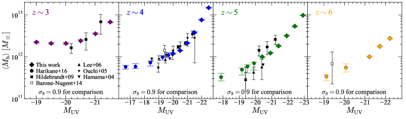
Figure 17.— Comparison of the mean dark matter halo masses, $\left<M_{\mathrm{h}}\right>$, with the literature under the same cosmology. We plot $M_{\mathrm{UV}}^{\mathrm{th}}$ as $M_{\mathrm{UV}}$. The diamonds represent the mean dark matter halo masses in this work with the cosmological parameters of $(h,\Omega_{\mathrm{m}},\Omega_{\mathrm{\Lambda}},\sigma_{8})=(0.7,0.3,0.7,0.9)$. The circles are the results of Harikane et al. (2016) with the same cosmology. The black symbols denote results of the previous studies. We plot the results of Hildebrandt et al. (2009, squares), Lee et al. (2006, upward triangles), Ouchi et al. (2005, stars), and Hamana et al. (2004, downward triangle). The downward triangles have no error bars, because Hamana et al. (2004) do not provide errors of the mean dark matter halo mass. We also show the results of Barone-Nugent et al. (2014) as black open squares, which are re-calcutaed with the cosmological parameters of $(h,\Omega_{\mathrm{m}},\Omega_{\mathrm{L}},\sigma_{8})=(0.7,0.3,0.7,0.9)$. The mean dark matter halo mass of the faintest subsample at $z\sim 3$ is slightly more massive than that of the next faintest subsample, because of the higher fraction of satellite galaxies that are typically reside in massive halos (see Table 8).

We find a redshift evolution of the $M_{\mathrm{UV}}-M_{\mathrm{h}}$ relation from $z\sim 1.7$ to $7$. For example, $M_{\mathrm{h}}$ monotonically decreases from $z\sim 7$ to $1.7$ (from $z\sim 6$ to $2.2$) by a factor of 5 (9) at $M_{\mathrm{UV}}=-19.5\ (-20.5)$. This redshift evolution indicates that the dust-uncorrected SFR increases with increasing redshift at fixed dark matter halo mass. We also plot the best-fit $M_{\mathrm{UV}}-M_{\mathrm{h}}$ relations at $z\sim 1.7$, $2.2$, $3$, $4$, $5$, $6$, and $7$ in Figure 16. These relations are expressed with the following double power law function:

$$M_{\mathrm{h}}=\frac{M_{\mathrm{h,0}}}{2}\left[10^{-0.4(M_{\mathrm{UV}}-M_{\mathrm{UV,0}})\alpha}+10^{-0.4(M_{\mathrm{UV}}-M_{\mathrm{UV,0}})\beta}\right]$$ (54)

where $M_{\mathrm{h,0}}$ and $M_{\mathrm{UV,0}}$ are characteristic halo mass and UV magnitude, respectively, and $\alpha$ and $\beta$ are faint and bright end power-law slopes, respectively. In Figure 16, we use parameter sets of $(\mathrm{log}M_{\mathrm{h,0}},M_{\mathrm{UV,0}},\alpha,\beta)=(11.67,-19.30,0.47,2.11)$, $(11.82,-19.77,0.61,2.34)$, $(12.05,-20.75,0.56,2.15)$, $(11.92,-20.90,0.60,2.29)$, $(11.62,-20.58,0.51,1.67)$, $(11.44,-20.35,0.36,1.54)$, and $(11.32,-20.35,0.36,1.54)$ for $z\sim 1.7$, $2.2$, $3$, $4$, $5$, $6$, and $7$, respectively. At $z\sim 7$, $M_{\mathrm{UV,0}}$, $\alpha$, and $\beta$ are fixed to the values at $z\sim 6$.

In Figure 17, we compare the mean halo masses, $\left<M_{\mathrm{h}}\right>$, of our subsamples with the literature. Because most of the previous studies assume the cosmological parameter set of $(\Omega_{\mathrm{m}},\Omega_{\mathrm{\Lambda}},h,\sigma_{8})=(0.3,0.7,0.7,0.9)$ that is different from our assumption, we obtain HOD model fitting results for our data with $(\Omega_{\mathrm{m}},\Omega_{\mathrm{\Lambda}},h,\sigma_{8})=(0.3,0.7,0.7,0.9)$ for comparison. Similarly, the results of the previous studies are re-calculated with the same cosmological parameter sets if different cosmological parameter set is assumed. In this way, we conduct our comparisons using an equivalent set of cosmological parameters across all datasets. In Figure 17, we find that our results at $z\sim 3$ and $4$ are consistent with those of the previous studies within the uncertainties. While the previous results at $z\sim 5$ are largely scattered, our $z\sim 5$ results are placed near the center of the distribution of the previous studies. At $z\sim 6$, our results agree with that of Barone-Nugent et al. (2014). In summary, our results are consistent with most of the previous studies. Furthermore, our results improve on both the statistics and the dynamic range covered in $M_{\mathrm{UV}}$.

5.4. $SFR/\dot{M}_{\mathrm{h}}-M_{\mathrm{h}}$ Relation

We estimate a ratio of the SFR to the dark matter accretion rate, $SFR/\dot{M}_{\mathrm{h}}$, or the baryon conversion efficiency, $SFR/(f_{\mathrm{b}}\dot{M}_{\mathrm{h}})$, where $f_{\mathrm{b}}=\Omega_{\mathrm{b}}/\Omega_{\mathrm{m}}$ is the cosmic baryon fraction. Since the baryon gas accretes into the halo together with dark matter, this ratio indicates the star formation efficiency. In this paper, the star formation efficiency indicates $SFR/\dot{M}_{\mathrm{h}}$ or $SFR/(f_{\mathrm{b}}\dot{M}_{\mathrm{h}})$, not the ratio of the SFR to the gas mass ($SFR/M_{\mathrm{gas}}$), which is usually used in radio astronomy. We derive the dust-uncorrected SFRs ($SFR_{\mathrm{UV}}$) from UV luminosities using the calibration used in Madau & Dickinson (2014) with the Salpeter (1955) IMF:

$$SFR_{\mathrm{UV}}\ (M_{\odot}\ \mathrm{yr}^{-1})=1.15\times 10^{-28}L_{\mathrm{UV}}\ (\mathrm{erg\ s^{-1}\ Hz^{-1}}).$$ (55)

We correct the SFR for the dust extinction using an attenuation-UV slope ($\beta_{\mathrm{UV}}$) relation (Meurer et al. 1999) and $\beta_{\mathrm{UV}}-M_{\mathrm{UV}}$ relation at each redshift. We use the $\beta_{\mathrm{UV}}-M_{\mathrm{UV}}$ relation in Bouwens et al. (2014) at $z\gtrsim 4$ and linearly extrapolate the relation with fixing the slope at $z\lesssim 4$. The estimated SFRs are presented in Table 8. We calculate $\dot{M}_{\mathrm{h}}$ as a function of halo mass and redshift using an analytic formula obtained from N-body simulation results in Behroozi & Silk (2015, Equation (B8)). Note that the accretion rates in Behroozi & Silk (2015) are typically $\sim 2$ times lower than those calculated based on Equations (E2)-(E6) in Behroozi et al. (2013), which are used in our previous work (Harikane et al. 2018a), because the Behroozi et al. (2013) accretion rates only trace the progenitors of $z=0$ halos.

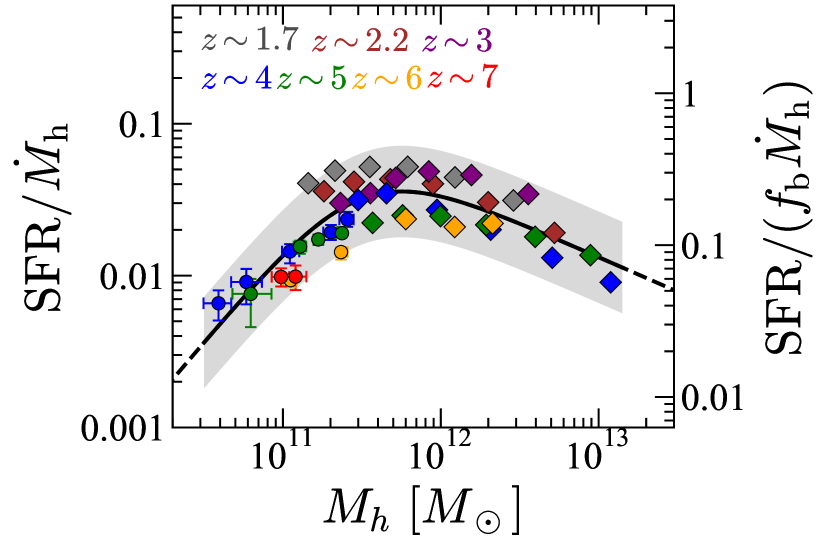
Figure 18.— $\mathrm{SFR}/\dot{M}_{\mathrm{h}}$ and baryon conversion efficiency ($\mathrm{SFR}/(f_{\mathrm{b}}\dot{M}_{\mathrm{h}})$) as a function of the halo mass. The gray, brown, purple, blue, green, orange, and red filled diamonds (circles) denote the ratios as a function of the halo mass, at $z\sim 1.7$, $2.2$, $3$, $4$, $5$, $6$, and $7$, respectively, for the subsamples in this work (in Harikane et al. 2016). The statistical errors for our data are smaller than the symbols (diamonds). The black solid curve is the fitting formulae of Equation (56) for the $SFR/\dot{M}_{\mathrm{h}}-M_{\mathrm{h}}$ relation at $z\sim 2-7$, and the gray shaded region represents the $2\sigma$ typical scatter ($0.3\ \mathrm{dex}$) of the data points compared to the relation.

We plot the dust-corrected $SFR/\dot{M}_{\mathrm{h}}$ ratios at $z\sim 2-7$ as a function of the halo mass in Figure 18. The results are also summarized in Table 9. The black solid curve in Figure 18 represents the following $SFR/\dot{M}_{\mathrm{h}}-M_{\mathrm{h}}$ relation:

$$\frac{SFR}{\dot{M}_{\mathrm{h}}}=\frac{2\times 3.2\times 10^{-2}}{(M_{\mathrm{h}}/10^{11.5})^{-1.2}+(M_{\mathrm{h}}/10^{11.5})^{0.5}}$$ (56)

This relation agrees with the measured $SFR/\dot{M}_{\mathrm{h}}$ ratios at $z\sim 2-7$ within 0.3 dex that is a typical $2\sigma$ scatter. This good agreement indicates that the star formation efficiency does not significantly change beyond 0.3 dex in the wide redshift range of $z\sim 2-7$, suggesting the existence of the fundamental relation between the star formation and the mass accretion (the growth of the galaxy and its dark matter halo assembly), as discussed in Harikane et al. (2018a) at $z\sim 4-7$ (see also Bian et al. 2013).

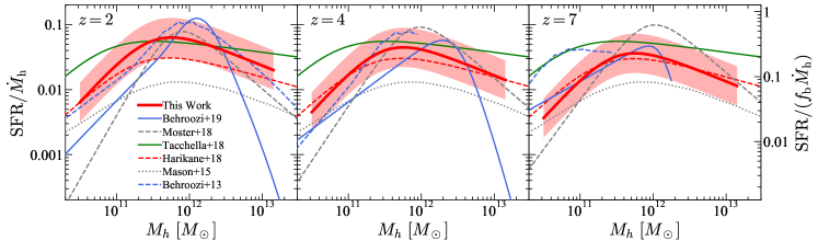
Figure 19.— Comparison of the $\mathrm{SFR}/\dot{M}_{\mathrm{h}}$ ratio with the literature. The red solid curve shows the redshift-dependent relation constrained in this work (Equation (57)), and the shaded region represents the $2\sigma$ typical uncertainties. Results compared include those from our previous work (Equation (25) in Harikane et al. 2018a, red dashed curve), Behroozi et al. (2019, blue solid curve), Moster et al. (2018, gray dashed curve), Tacchella et al. (2018, green solid curve), Mason et al. (2015a, gray dotted curve), and Behroozi et al. (2013, blue dashed curve). All results are converted to use the Salpeter (1955) IMF (equation (55)). The result of Harikane et al. (2018a) is re-calculated based on the accretion rate of Behroozi & Silk (2015), and thus is $\sim 2$ times higher than the original relation in Harikane et al. (2018a).

On the other hand, the $SFR/\dot{M}_{\mathrm{h}}$ ratio gradually increases with increasing redshift within 0.3 dex from $z\sim 5$ to $1.7$. If we take this possible evolution into account, the ratio can be expressed as,

$$\frac{SFR}{\dot{M}_{\mathrm{h}}} = \frac{2\times 3.2\times 10^{-2}}{(M_{\mathrm{h}}/10^{11.5})^{-1.2}+(M_{\mathrm{h}}/10^{11.5})^{0.5}}$$ (57)

$$\times(0.53\,\mathrm{tanh}[0.54(2.9-z)]+1.53)\ \ \ \ \$$

This relation indicates that the star formation efficiency does not significantly change from $z\sim 7$ to $5$, and then gradually increases within a factor of $\sim 2$ from $z\sim 5$ to $1.7$, still consistent with the results of Harikane et al. (2018a), who have identified redshift-independent relation at $z\sim 4-7$ within 0.15 dex. The reason for this elevated efficiency at $z<5$ is not clear. One possibility is an increase of the metallicity in galaxies toward lower redshift, resulting in more efficient gas cooling.

In Figure 19, we compare our $\mathrm{SFR}/\dot{M}_{\mathrm{h}}-M_{\mathrm{h}}$ relation with results in the literature (Behroozi et al. 2013; Mason et al. 2015a; Harikane et al. 2018a; Tacchella et al. 2018; Moster et al. 2018; Behroozi et al. 2019). The relations in the literature show similar trends to our result; the $\mathrm{SFR}/\dot{M}_{\mathrm{h}}$ ratio has a peak of $\mathrm{SFR}/\dot{M}_{\mathrm{h}}\sim 0.1-0.01$ around the halo mass of $10^{11}-10^{12}\ M_{\odot}$. However, the slopes of the relation at the high-mass and low-mass ends are different between these studies. These differences are possibly due to differences in used observational datasets, the halo mass functions, and details of modeling. We also note that there are several systematic uncertainties on the $\mathrm{SFR}/\dot{M}_{\mathrm{h}}$ measurements. Assumptions on the IMF and dust attenuation have impacts on the SFR. The conversion factor between the SFR and UV luminosity (Equation (55)) depends on the stellar age and metallicity (e.g., Madau & Dickinson 2014).

6. Discussion

6.1. Physical Origin of the Cosmic SFR Density Evolution

In Section 5.4, we find the fundamental $SFR/\dot{M}_{\mathrm{h}}-M_{\mathrm{h}}$ relation; the value of $SFR/\dot{M}_{\mathrm{h}}$ at fixed $M_{\mathrm{h}}$ does not significantly change beyond $0.3\ \mathrm{dex}$ at $z\sim 2-7$. We examine whether this fundamental $SFR/\dot{M}_{\mathrm{h}}-M_{\mathrm{h}}$ relation is consistent with the observational results, i.e., cosmic SFR densities and the UV luminosity functions. We calculate the cosmic SFR density as follows:

$$\rho_{\mathrm{SFR}}=\int dM_{\mathrm{h}}\frac{dn}{dM_{\mathrm{h}}}SFR=\int dM_{\mathrm{h}}\frac{dn}{dM_{\mathrm{h}}}\dot{M}_{\mathrm{h}}\frac{SFR}{\dot{M}_{\mathrm{h}}},$$ (58)

where $SFR/\dot{M}_{\mathrm{h}}$ at $z\sim 2-7$ is obtained as a function of $M_{\mathrm{h}}$ in Section 5.4 (Equations (56) or (57)). We integrate down to the halo mass corresponding to the SFR of $0.3\ M_{\odot}\ \mathrm{yr^{-1}}$ ($M_{\mathrm{UV}}=-17$ mag with the Madau & Dickinson 2014 calibration), as previous studies (Bouwens et al. 2015, 2020; Finkelstein et al. 2015b; Oesch et al. 2018).

Figure 20.— Cosmic SFR density. The bottom panel shows the comparison of the cosmic SFR densities. The red curves with the shade represent cosmic SFR densities derived from Equation (58). For the solid and dashed lines, we assume the redshift-dependent and independent $SFR/\dot{M}_{\mathrm{h}}-M_{\mathrm{h}}$ relations (Equations (57) and (56)), respectively, which are constrained in this paper at $2\lesssim z\lesssim 7$. The shaded regions correspond to the $1\sigma$ (0.15 dex) scatter in the $SFR/\dot{M}_{\mathrm{h}}-M_{\mathrm{h}}$ relation. We integrate down to the halo mass corresponding to the SFR of $0.3\ M_{\odot}\ \mathrm{yr^{-1}}$ ($M_{\mathrm{UV}}=-17$ mag with the Madau & Dickinson 2014 calibration), as previous studies (Bouwens et al. 2015, 2020; Finkelstein et al. 2015b; Oesch et al. 2018). The black circles show observed cosmic SFR densities taken from Madau & Dickinson (2014), Finkelstein et al. (2015b), McLeod et al. (2016), and Bouwens et al. (2020). All results are converted to use the calibration of Madau & Dickinson (2014) with the Salpeter (1955) IMF (Equation (55)). The top panel shows $\Delta\frac{SFR}{\dot{M}_{\mathrm{h}}}=\frac{SFR}{\dot{M}_{\mathrm{h}}}(z)/\frac{SFR}{\dot{M}_{\mathrm{h}}}(z=5)$ at a given halo mass. The sold and dashed curves are calculated with Equations (57) and (56), respectively.

Firstly we assume the redshift-independent $SFR/\dot{M}_{\mathrm{h}}-M_{\mathrm{h}}$ relation (Equation (56)). Figure 20 compares our calculated SFR densities (the dashed curve) with observational results in the literature (Madau & Dickinson 2014; Finkelstein et al. 2015b; McLeod et al. 2016; Oesch et al. 2018; Bouwens et al. 2020). The results in the literature are all converted to use the calibration of Madau & Dickinson (2014) with the Salpeter (1955) IMF (Equation (55)). We find that our calculation well reproduces the overall trend of the cosmic SFR density evolution; the calculated density increases from $z\sim 10$ to $4-2$, and decreases from $z\sim 4-2$ to $0$. However, the SFR densities are underpredicted compared to the observations at $z\sim 1-2$ by $\sim 0.3$ dex.

Then we use the gradually evolving $SFR/\dot{M}_{\mathrm{h}}-M_{\mathrm{h}}$ relation (Equation (57)), instead of Equation (56). As shown in Figure 20, our calculated cosmic SFR densities (the solid curve) based on Equation (57) agree well with the observations especially at $z\sim 1-2$, compared to the calculation based on the redshift-independent relation (the dashed curve). Quantitatively, the reduced $\chi^{2}$ value improves significantly from $\chi^{2}/\mathrm{dof}=25.4$ to $3.0$. These analyses indicate that the overall trend of the redshift evolution can be reproduced by the redshift-independent $SFR/\dot{M}_{\mathrm{h}}-M_{\mathrm{h}}$ relation (Equation (56)), but the gradual increase of the star formation efficiency at $z<5$ (Equation (57)) is needed to quantitatively reproduce the observed SFR densities. Note that we have constrained the $SFR/\dot{M}_{\mathrm{h}}-M_{\mathrm{h}}$ relations by using normal star forming galaxies (dropout, BX, and BM galaxies), and not considered quiescent or dusty starburst galaxies. Quiescent and dusty starburst galaxies are expected to have lower and higher $SFR/\dot{M}_{\mathrm{h}}$ ratios than the normal star forming galaxies, and effects of these galaxies are thought to be less dominant at $z\gtrsim 4$ (e.g., Muzzin et al. 2013; Bouwens et al. 2020; Fudamoto et al. 2021). Although quiescent and dusty starburst galaxies would be non-negligible at $z\lesssim 3$, the good agreement at $z\sim 1-2$ still indicates that the star formation efficiency averaged over all galaxy populations gradually increases at $z<5$, as long as the observed SFR densities (including the treatment of the dust extinction correction) are correct.

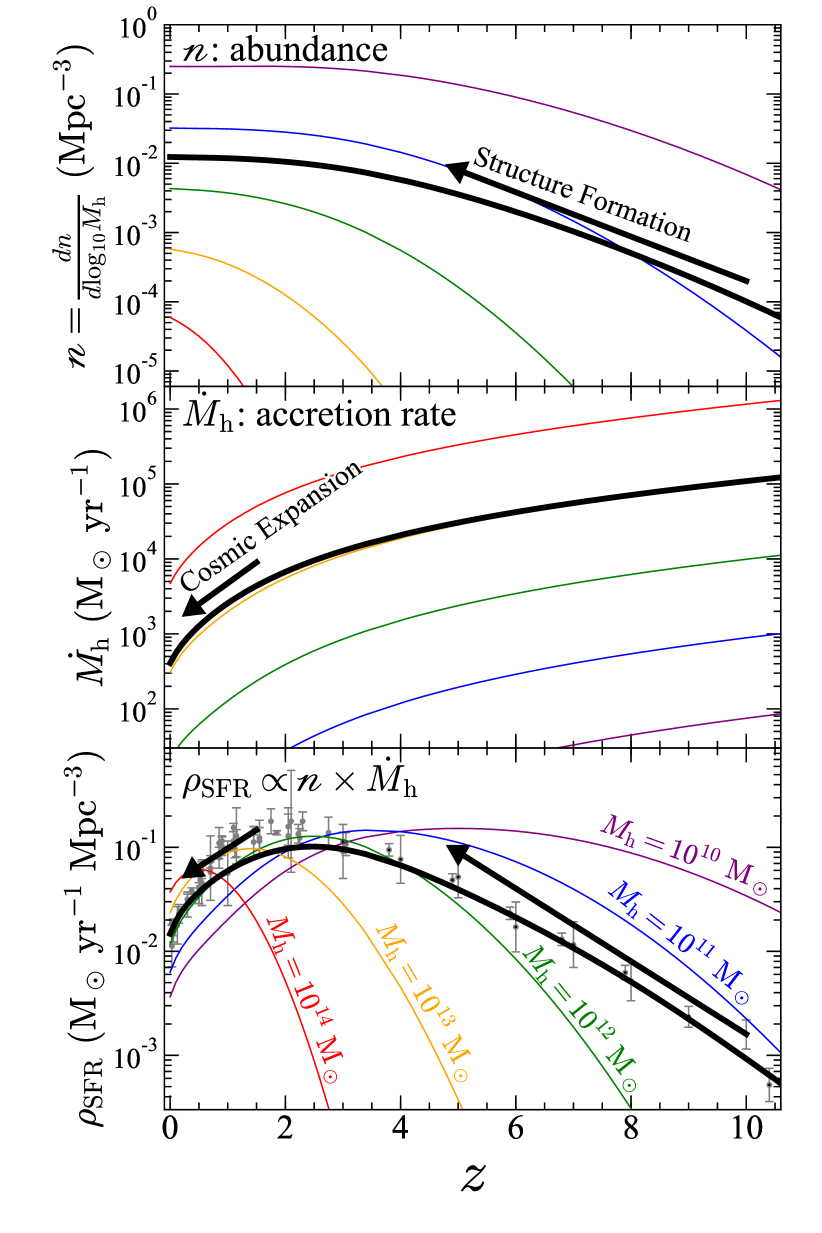
Figure 21.— Mechanism of the cosmic SFR density evolution. Top panel: the purple, blue, green, orange, and red curves indicate the number density of halos whose masses are $M_{\mathrm{h}}=10^{10}$, $10^{11}$, $10^{12}$, $10^{13}$, and $10^{14}\ M_{\odot}$, respectively. The number density is calculated by using the Behroozi et al. (2013) halo mass function. The black curve represents a weighted number density based on Equation (57). Middle panel: same as the top panel but for the dark matter accretion rate calculated by using the formula in Behroozi & Silk (2015). Bottom panel: same as the top panel but for the cosmic SFR density. The gray circles are observed cosmic SFR densities taken from Madau & Dickinson (2014), Finkelstein et al. (2015b), McLeod et al. (2016), and Bouwens et al. (2020). Since the cosmic SFR density at a given halo mass is proportional to the galaxy (halo) number densities and SFRs (accretion rates) as shown in Equation (58), the redshift evolution of the cosmic SFR density is made by the monotonic steep increase of the halo number density from $z\sim 10$ to $z\sim 4$ and the monotonic decrease of the accretion rate from $z\sim 2$ to $z\sim 0$, resulting a peak of the SFR density around $z\sim 2-3$.

The good agreement with the overall trend indicates that the evolution of the cosmic SFR densities is primarily driven by the monotonic increase of the halo number density and the monotonic decrease of the accretion rate, given the weak redshift evolution of the $SFR/\dot{M}_{\mathrm{h}}-M_{\mathrm{h}}$ relation, as discussed in Harikane et al. (2018a). The number density of halos at a given halo mass increases due to structure formation from $z\sim 10$ to a certain redshift at $z\lesssim 4$ depending on the mass and then becomes almost constant after that (the top panel in Figure 21), resulting in the increase of the galaxy number density from $z\sim 10$ to $z\lesssim 4$. The dark matter (and gas) accretion rate monotonically decreases over the whole redshift range due to the cosmic expansion, with a steep drop from $z\sim 2$ to $0$ (the middle panel in Figure 21), resulting in the monotonic decrease SFR of each galaxy at a given halo mass. Because the cosmic SFR density at a given halo mass is proportional to the number density and mass accretion rate (or SFR) as shown in Equation (58), the calculated cosmic SFR density has a peak at $z\sim 2-3$ (the bottom panel in Figure 21). More specifically, the product of the number density and mass accretion rate for each halo mass has a peak at a certain redshift due to the increase of the number density and decrease of the accretion rate, with the peak redshift depending on the halo mass, and the $SFR/\dot{M}_{\odot}-M_{\mathrm{h}}$ relation determines the peak redshift of the cosmic SFR density integrated over the halo mass, as shown in the bottom panel in Figure 21).

In our calculation we integrate Equation (58) down to the SFR of $0.3\ M_{\odot}\ \mathrm{yr^{-1}}$, corresponding to the halo mass of $\sim 3\times 10^{10}\ M_{\odot}$ at $z\sim 7$. This integration limit is chosen to match the calculations at $z\gtrsim 2$ in previous studies (Bouwens et al. 2015, 2020; Finkelstein et al. 2015b; Oesch et al. 2018), and slightly different from the calculations in Madau & Dickinson (2014), who integrate down to $0.03L^{*}$. This difference does not affect our discussions above. Bouwens et al. (2021) show that the $M_{\mathrm{UV}}^{*}$ parameter of the luminosity function is almost constant ($M_{\mathrm{UV}}^{*}\sim-21$ mag) from $z\sim 8$ to $2$, and then decreases to $M_{\mathrm{UV}}^{*}\sim-18$ mag toward $z\sim 0$. At $z\sim 2-8$, the SFR corresponding to $0.03L^{*}$ with $M_{\mathrm{UV}}^{*}=-21$ mag is roughly $0.5\ M_{\odot}\ \mathrm{yr^{-1}}$, comparable to our integration limit. Below $z\sim 2$, the corresponding SFR is smaller than our limit, e.g., $0.03\ M_{\odot}\ \mathrm{yr^{-1}}$ with $M_{\mathrm{UV}}^{*}\sim-18$ mag at $z\sim 0$. However, even if we integrate Equation (58) down to this SFR limit, the calculated cosmic SFR density increases only by 0.1 dex at $z<3$, and cannot explain the 0.3 dex difference between the observed SFR densities and the dashed curve in Figure 20.

We also calculate the UV luminosity function at each redshift as follows:

$$\Phi(M_{\mathrm{UV}})=\frac{dn}{dM_{\mathrm{h}}}\frac{dM_{\mathrm{h}}}{dM_{\mathrm{UV}}}.$$ (59)

From Equation (57), we can obtain the $M_{\mathrm{UV}}-M_{\mathrm{h}}$ relation and $\frac{dM_{\mathrm{h}}}{dM_{\mathrm{UV}}}$ at each redshift, since $\dot{M}_{\mathrm{h}}$ can be expressed as a function of $M_{\mathrm{h}}$ and $z$ (Behroozi & Silk 2015). Note that $M_{\mathrm{UV}}$ is the observed absolute magnitude after dust extinction assuming the attenuation-UV slope ($\beta_{\mathrm{UV}}$) relation (Meurer et al. 1999) and $\beta_{\mathrm{UV}}-M_{\mathrm{UV}}$ relations (Bouwens et al. 2014). We correct for satellite galaxies using satellite fractions measured in previous studies (Wake et al. 2011; Martinez-Manso et al. 2015; McCracken et al. 2015; Harikane et al. 2016, 2018a), although the correction is not large at high redshift. The calculated UV luminosity functions at $z\sim 0-10$ are plotted in Figure 22. We find that the calculated luminosity functions are in rough agreement with observed results given the $0.15\ \mathrm{dex}$ ($1\sigma$) uncertainty in $SFR/\dot{M}_{\mathrm{h}}$, indicating that our $SFR/\dot{M}_{\mathrm{h}}-M_{\mathrm{h}}$ relation is consistent with the observed redshift evolution of the UV luminosity function.

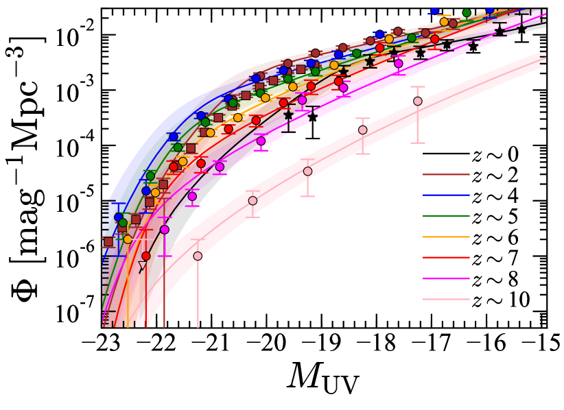
Figure 22.— Comparison of the rest-frame UV luminosity functions. Solid curves are the calculated luminosity functions from Equation (59) with the $\mathrm{SFR}/\dot{M}_{\mathrm{h}}-M_{\mathrm{h}}$ relation of Equation (57). The points show the observed galaxy luminosity functions of Bouwens et al. (2021, circles), Moutard et al. (2020, squares), and Arnouts et al. (2005, stars). The shaded regions correspond to the $1\sigma$ (0.15 dex) scatter in the $SFR/\dot{M}_{\mathrm{h}}-M_{\mathrm{h}}$ relation.

Mason et al. (2015a) and Tacchella et al. (2018) also report that the constant star formation efficiency model can reproduce the UV luminosity functions at $z\gtrsim 4$. This is consistent with our results of the $SFR/\dot{M}_{\mathrm{h}}-M_{\mathrm{h}}$ relation in this study and our previous work (Harikane et al. 2018a). Bouwens et al. (2021) claim that the evolution of the luminosity function at $z\sim 2.5-10$ can be explained by the halo mass function and the constant star formation efficiency model. This is qualitatively consistent with our results, but the gradual increase of the star formation efficiency at $z<5$ is needed to quantitatively reproduce the redshift evolution of the cosmic SFR density, as discussed above.

6.2. Future Prospects for Star Formation at $z>10$

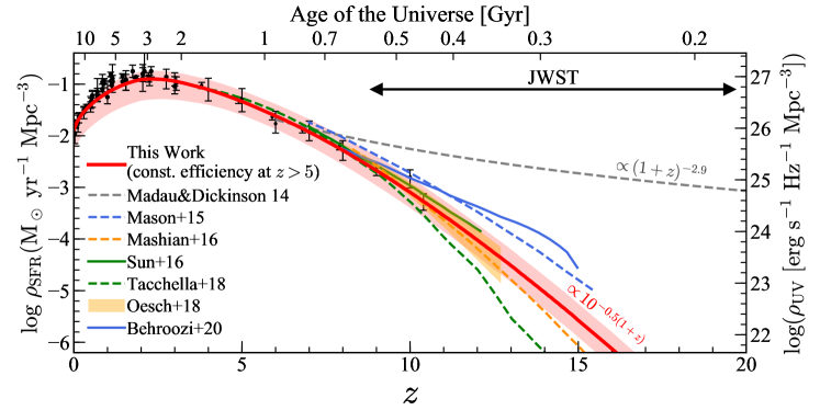
Figure 23.— Comparison of the cosmic SFR density at $z>7$. The red curve with the shade represents the cosmic SFR density calculated in this work based on the constant star formation efficiency at $z>5$ (Equation (57)), integrated down to the SFR of $0.3\ M_{\odot}\ \mathrm{yr^{-1}}$ ($M_{\mathrm{UV}}=-17$ mag), as previous studies (Bouwens et al. 2015, 2020; Finkelstein et al. 2015b; Oesch et al. 2018). The gray dashed curve shows the extrapolation of the relation of Madau & Dickinson (2014) at $z>6$. The other curves show predictions from models of Mason et al. (2015a, blue dashed curve), Mashian et al. (2016, orange dashed curve), Sun & Furlanetto (2016, green solid curve), Tacchella et al. (2018, green dashed curve), and Behroozi et al. (2020, blue solid curve). The orange shaded region indicates a prediction of the halo evolution model in Oesch et al. (2018). All results are converted to use the Salpeter (1955) IMF (equation (55)).

In the previous section, we show that the constant star formation efficiency (Equation (56)) can reproduce the evolution of the cosmic SFR density at $5\lesssim z\lesssim 10$. By assuming that this $SFR/\dot{M}_{\mathrm{h}}-M_{\mathrm{h}}$ relation does not evolve to higher redshifts, we can predict the cosmic SFR density at $z>10$ based on the evolution of the halo mass function and dark matter accretion rate.

Figure 23 compares our calculated SFR densities (the red curve) with predictions from models in the literature (Mason et al. 2015a, Mashian et al. 2016, Sun & Furlanetto 2016, Tacchella et al. 2018, Oesch et al. 2018, and Behroozi et al. 2020). We find that the cosmic SFR density based on the constant star formation efficiency rapidly decreases with increasing redshift as $\propto 10^{-0.5(1+z)}$, similar to the predictions of other models. More quantitatively, the SFR densities from observations at $z\lesssim 10$ and our predictions at $z\gtrsim 10$ are well-fitted with the following function:

$$\rho_{\mathrm{SFR}}/[\mathrm{M_{\odot}\ \mathrm{yr^{-1}}\ \mathrm{Mpc^{-3}}}]$$

$$=\frac{1}{61.7\times(1+z)^{-3.13}+1.0\times 10^{0.22(1+z)}+2.4\times 10^{0.50(1+z)-3.0}},$$ (60)

as shown in Figure 24. This is contrast to the extrapolation of the fitting function in Madau & Dickinson (2014) that shows a smooth decline as $\propto(1+z)^{-2.9}$ at $z>10$ (the gray dashed curve in Figures 23 and 24), and possible estimates of the SFR densities at $z>12$ based on $z\sim 6$ passive galaxies in Mawatari et al. (2020). James Webb Space Telescope (JWST) will allow us to directly observe galaxies at $z\sim 10-20$, and investigate whether the SFR density rapidly decreases as predicted in many models or not, providing insights into star formation efficiencies in $z\sim 10-20$ galaxies.

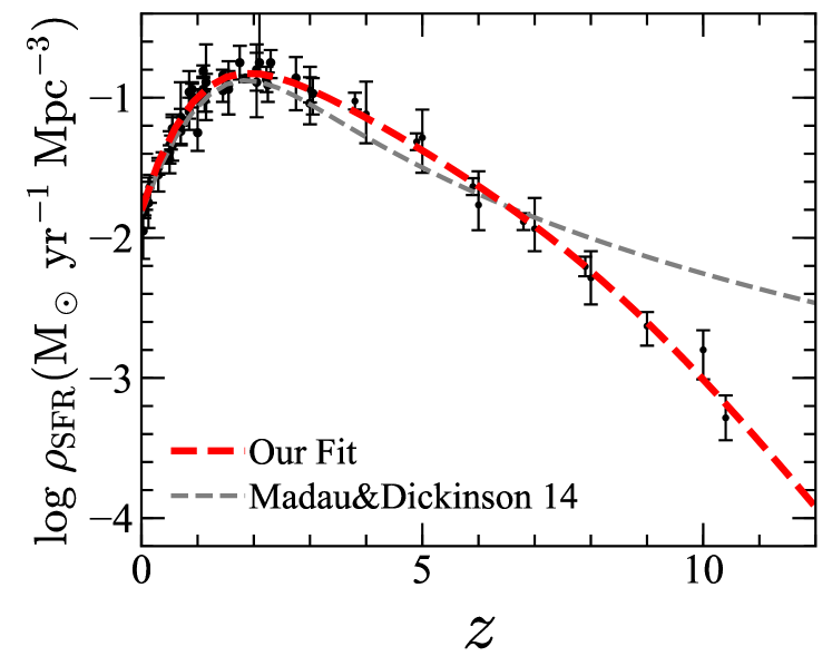
Figure 24.— Fit to the observed cosmic SFR densities. The red dashed curve represents our fit (Equation (60)) to the observed cosmic SFR densities at $z\lesssim 10$ and the calculated SFR densities at $z>10$ in this work. The gray dashed curve shows the fit in Madau & Dickinson (2014). All results are converted to use the Salpeter (1955) IMF (equation (55)).

Using this method to predict the SFR density at $z>10$, we can obtain a rough estimate of the epoch of the first star formation. We calculate the cumulative number of formed stars as a function of redshift:

$$N_{\mathrm{star}}(z)=V_{\mathrm{survey}}\int^{t(z)}_{{t(z)}-t_{\mathrm{LF}}}\!\!\!dt\rho_{\mathrm{SFR}}/M_{\mathrm{FS}},$$ (61)

where $V_{\mathrm{survey}}$ is the survey volume, $t_{\mathrm{LF}}$ is the typical lifetime of the star, and $M_{\mathrm{FS}}$ is a typical mass of the first star. Here we assume $t_{\mathrm{LF}}=3\ \mathrm{Myr}$ (Schaerer 2002) and $M_{\mathrm{FS}}=100\ M_{\odot}$ (e.g., Hirano et al. 2015). We adopt $V_{\mathrm{survey}}=(3\ h^{-1}\mathrm{Mpc})^{3}$ that is the volume of the simulation box in Hirano et al. (2015). We calculate $\rho_{\mathrm{SFR}}$ using Equation (58) by extrapolating the $SFR/\dot{M}_{\mathrm{h}}-M_{\mathrm{h}}$ relation both to the higher redshift and lower mass range. We integrate down to the halo mass of $10^{5}\ M_{\odot}$, comparable to halo masses of first stars in simulations (e.g., Hirano et al. 2015). Figure 25 shows the calculated cumulative number of formed stars. The shaded region indicates possible uncertainties of the low-mass slope of the $SFR/\dot{M}_{\mathrm{h}}-M_{\mathrm{h}}$ relation and the mass limit of the integration that we adopt $10^{4}-10^{6}\ M_{\odot}$. The number reaches 1 around $z\sim 16-27$, implying the first star formation in this epoch. This formation epoch agrees with theoretical simulations (Hirano et al. 2014, 2015), although this is a very rough estimate. Especially, it is not clear whether the assumed $SFR/\dot{M}_{\mathrm{h}}-M_{\mathrm{h}}$ relation holds at $z>10$ or not, because physics in the first star formation are expected to be different from star/galaxy formation at the epoch we currently observe due to the evolution of physical parameters such as metallicity.

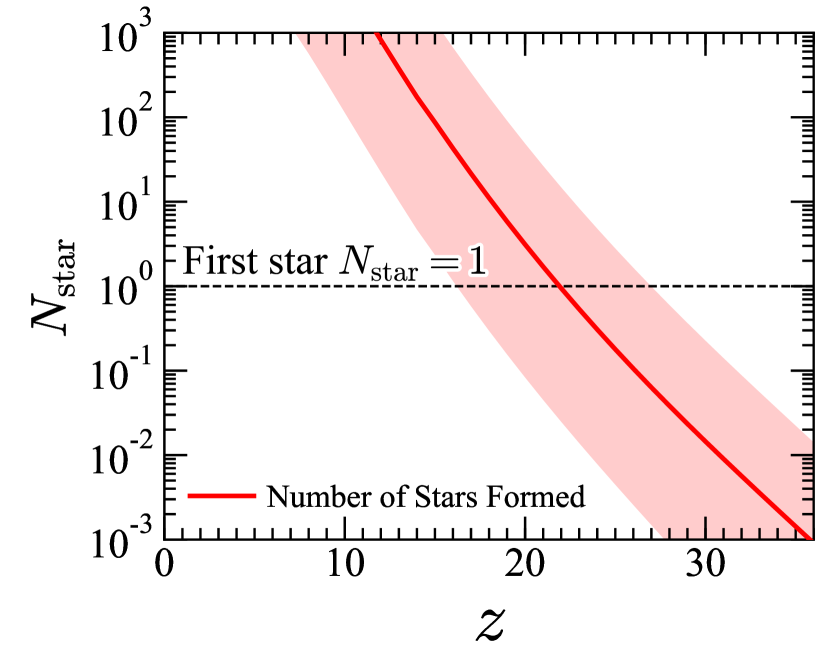
Figure 25.— Cumulative number of formed stars as a function of the redshift. The red line shows the cumulative number of formed stars calculated based on the SFR density (Equation (61)). We extrapolate the $SFR/\dot{M}_{\mathrm{h}}-M_{\mathrm{h}}$ relation both to the higher redshift and lower mass range, and the shaded region indicates possible uncertainties of the $SFR/\dot{M}_{\mathrm{h}}$ ratio and the mass limit of the integration. The cumulative number reaches 1 around $z\sim 16-27$, implying the first star formation at this epoch.

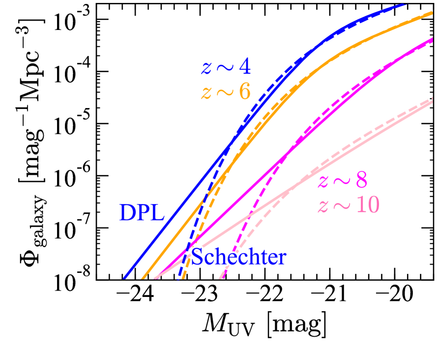
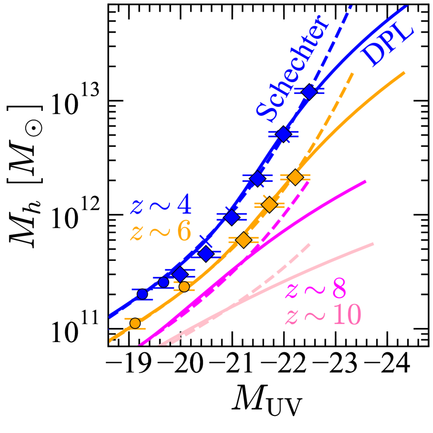
Figure 26.— Galaxy luminosity function (left), $M_{\mathrm{UV}}-M_{\mathrm{h}}$ relation (middle), and star formation efficiency ($SFR/\dot{M}_{\mathrm{h}}-M_{\mathrm{h}}$ relation, right) in cases of the DPL and Schechter luminosity functions. The blue, orange, magenta, and pink solid (dashed) lines represent relations in the case of the DPL (Schechter) luminosity functions at $z\sim 4$, $6$, $8$, and $10$, respectively. To reproduce the observed bright end excess of the number density like the DPL function (the solid line in the left panel), the higher star formation efficiency (the solid line in the right panel) is needed at the massive end, compared to the case of the Schechter function (the dashed line). The blue and orange symbols in the middle panel show the results of this study (diamonds), Harikane et al. (2018a, crosses), and Harikane et al. (2016, circles). In the right panel, the black solid curve is the fitting formulae of Equation (56), and the gray shaded region represents the $2\sigma$ typical scatter ($0.3\ \mathrm{dex}$).

6.3. Origin of the Bright End Excess of the Galaxy Luminosity Function

As presented in Section 4.2.2, the obtained galaxy UV luminosity functions cannot be explained by the Schechter functions at the bright end ($M_{\mathrm{UV}}\lesssim-23$ mag), indicating the existence of the bright end excess of the number density beyond the Schechter function. Since these luminosity functions are estimated based on the spectroscopic galaxy fractions, the bright end excess cannot be explained by apparent AGNs (e.g., quasars). Here we discuss the following five possibilities for the origin of the bright end excess, (A) lensed galaxies, (B) mergers, (C) inefficient mass quenching, (D) low dust obscuration and (E) hidden AGN activity.

• Lensed galaxies. In Section 4.2.2, the lensed Schechter function can provide better fits than the Schechter functions. This indicates that the bright end excess can be explained by gravitationally lensed galaxies that are apparently bright. However, in our visual inspection of galaxies located at the bright end, we do not find a significant number of lensed galaxies that show elongated morphologies. In addition, the $z\sim 4$ luminosity function still shows the bright end excess at the $2.5-2.7\sigma$ levels beyond the lensed Schechter function, similar to the results of Ono et al. (2018). As discussed in Section 4.2.2, the calculated lensed Schechter function is an upper limit, because some fraction of lensed galaxies might be too close to foreground lensing galaxies to be selected as dropouts in our samples. Thus the bright end excess does not seem to be easily explained by lensed galaxies, although high spatial resolution images are required to draw definitive conclusions.

• Mergers. Some studies suggest that the major merger at high redshift is an important phase for formation of massive galaxies (e.g., Sawicki et al. 2020). Due to the limited spatial resolutions of the HSC images, some merging galaxies are not resolved and look like one bright galaxy. If most of galaxies at the bright end turn out to be merging galaxies, the bright end excess can be explained by merging galaxies. High spatial resolution images such as those obtained by Hubble are indeed useful to investigate this possibility (Bowler et al. 2017), but only a small fraction of our sources are observed with Hubble. Instead, Shibuya et al. (2021) have made high spatial resolution images by using the super-resolution technique, and estimate a major merger fraction of bright galaxies in galaxy samples of Ono et al. (2018). They find that the major merger fraction is $10-70\%$ for bright galaxies ($-24\lesssim M_{\mathrm{UV}}\lesssim-22$ mag) at $z\sim 4-7$. This can partly explain the number density excess of relatively bright galaxies ($M_{\mathrm{UV}}\gtrsim-23.6$ mag), but is not sufficient to explain the excess of very bright galaxies ($M_{\mathrm{UV}}\lesssim-23.6$ mag). Thus, it seems that the bright end excess cannot be explained by mergers.

• Inefficient mass quenching. It is thought that the exponential cutoff at the bright end of the Schechter function is caused by the mass quenching that suppresses star formation activity in massive halos (e.g., AGN feedback, virial shock heating). Thus the bright end excess beyond the Schechter function implies inefficient mass quenching in these high redshift bright galaxies as discussed in Ono et al. (2018) and Bowler et al. (2020). To investigate this possibility, we obtain the star formation efficiency, $SFR/\dot{M}_{\mathrm{h}}$, as a function of the halo mass in cases of the Schechter and DPL luminosity functions. Using the halo mass function and galaxy luminosity function, we obtain the $M_{\mathrm{UV}}-M_{\mathrm{h}}$ relation by the abundance matching technique:

  $$\int^{\infty}_{M_{\mathrm{h}}}dM^{\prime}_{\mathrm{h}}\frac{dn}{dM_{\mathrm{h}}}(M^{\prime}_{\mathrm{h}},z)(1+f_{\mathrm{sat}})$$

  $$=\int^{M_{\mathrm{UV}}}_{-\infty}dM^{\prime}_{\mathrm{UV}}\Phi_{\mathrm{galaxy}}(M^{\prime}_{\mathrm{UV}},z).$$ (62)

  Then we calculate the SFR and mass accretion rate in the same manner as Section 5.4, and obtain the $SFR/\dot{M}_{\mathrm{h}}$ ratio.

  Figure 26 presents the luminosity function, the $M_{\mathrm{UV}}-M_{\mathrm{h}}$ relation, and the star formation efficiency (the $SFR/\dot{M}_{\mathrm{h}}-M_{\mathrm{h}}$ relation) in cases of the DPL and Schechter functions at $z\sim 4$, $6$, $8$, and $10$. We find that estimated halo masses from our abundance matching agree well with those from the clustering analysis (the middle panel in Figure 26), as discussed in Harikane et al. (2016). If we assume the steep decline of the star formation efficiency ($SFR/\dot{M}_{\mathrm{h}}$) toward the massive end (the dashed line in the right panel), the calculated number density shows the exponential decline at the bright end similar to the Schechter function (the dashed line in the left panel), and cannot reproduce the excess of the observed number densities. To reproduce the bright end excess of the number density like the DPL function (the solid line in the left panel), higher star formation efficiencies are needed at the massive end (the solid line in the right panel), compared to the case of the Schechter function. For example, $\sim 2$ times higher star formation efficiency is needed in halos of $M_{\mathrm{h}}\simeq 10^{13}\ (10^{12})\ M_{\odot}$ at $z\sim 6$ (8). The high star formation efficiency at the bright end can be made by the inefficient mass quenching. Indeed the mass quenching is expected to be less efficient at higher redshift because of the shorter time scale of gas cooling and/or weaker AGN feedback due to the decreasing number of AGNs (i.e., quasar luminosity function) as discussed in Section 4.1.4.

• Low dust obscuration. Bowler et al. (2020) discuss the possibility that the intrinsic (without dust attenuation) UV luminosity function has a shallower decline at the bright end, and the dust obscuration controls the shape of the luminosity function. In the calculations above (C), we assume the attenuation-$\beta_{\mathrm{UV}}$ relation in Meurer et al. (1999) and the $\beta_{\mathrm{UV}}-M_{\mathrm{UV}}$ relations in Bouwens et al. (2014). However, the attenuation curve of high redshift galaxies is not well-understood (e.g., Hashimoto et al. 2019; Fudamoto et al. 2020; Harikane et al. 2020b; Bakx et al. 2020), and the $\beta_{\mathrm{UV}}-M_{\mathrm{UV}}$ relation is not well-constrained at this very bright magnitude range (i.e., $\sim-23$ mag). In addition, some recent studies report dust-poor UV luminous star forming galaxies at $z>2$ (Marques-Chaves et al. 2020, 2021). Thus it is possible that the dust obscuration in these bright galaxies is lower than what we assumed, resulting the bright end excess beyond the Schechter function.

• Hidden AGN activity. Although we subtract the number density of AGNs by the spectroscopic galaxy fractions, it is possible that there are still hidden AGNs in the galaxy luminosity function. UV luminosities of such hidden AGNs could be boosted due to AGN activity (e.g., Kim & Im 2021), resulting in the bright end excess. AGN activity of such sources can be probed only by deep spectroscopy covering several high ionization lines. Indeed, some studies report possible AGN activity in bright ($M_{\mathrm{UV}}\lesssim-22$ mag) galaxies at $z\gtrsim 7$ (e.g., Laporte et al. 2017; Mainali et al. 2018; Jiang et al. 2021; Endsley et al. 2021; Onoue et al. 2021). Since we do not know the fraction of such hidden AGNs in our sample due to the lack of deep spectroscopic data at the bright end, we cannot rule out the possibility that hidden AGNs make the bright end excess.

Based on these discussions above, we conclude that the bright end excess is possibly made by (C) inefficient mass quenching, (D) low dust obscuration and/or (E) hidden AGN activity, although it is possible that the dominant effect in making the bright end excess changes with redshift. We cannot distinguish these possibilities with the current datasets, and future large and deep observations are needed. For example, Euclid and Nancy Grace Roman Space Telescope can identify a large number of high redshift galaxies located at the bright end, allowing us to investigate the clustering and the star formation efficiency of such bright galaxies. ALMA follow-up observations for a statistical sample of bright galaxies will reveal the typical dust properties of these galaxies. Deep spectroscopy for a large number of bright galaxies with Subaru/PFS will allow us to investigate hidden AGN activity in such bright galaxies.

7. Summary

In this paper, we have identified 1,978,462 dropout candidates at $z\sim 4-7$ from $\sim 300$ deg² deep optical imaging data obtained in the HSC-SSP survey. Among these dropout candidates, 1037 dropouts are spectroscopically identified in our follow-up observations and the literature. Typical contamination rates are $<20\%$ and $<40\%$ at $z\sim 4-5$ and $z\sim 6-7$, respectively. Combined with $z\sim 2-3$ galaxy samples, we have a total of 4,100,221 sources at $z\sim 2-7$, which is the largest sample of high redshift galaxies to date. Using this sample, we have calculated the luminosity functions and angular correlation functions, and investigated statistical properties of these sources.

Our major findings are summarized below:

1. We have obtained rest-frame UV luminosity functions at $z\sim 4-7$ (Figures 5 and 6). Combined with results based on the complementary ultra-deep Hubble data and wide-area SDSS data, we have probed the luminosity function in a very wide UV magnitude range of $-29\lesssim M_{\mathrm{UV}}\lesssim-14$ mag, corresponding to the luminosity range of $0.002L^{*}_{\mathrm{UV}}\lesssim L_{\mathrm{UV}}\lesssim 2000L^{*}_{\mathrm{UV}}$.

2. Spectroscopic galaxy fractions indicate that most of the sources are AGNs (galaxies) at $M_{\mathrm{UV}}<-24$ ($M_{\mathrm{UV}}>-22$) mag (Figures 5 and 6). We have found that the luminosity function in this very wide magnitude range can be well-fitted by the DPL+DPL or DPL+Schechter functions (Figure 7), indicating that the dropout luminosity function is a superposition of the AGN luminosity function (dominant at the bright end) and the galaxy luminosity function (dominant at the faint end).

3. We have estimated the galaxy luminosity functions by subtracting the AGN contributions using the spectroscopic galaxy fractions. The obtained galaxy luminosity functions show the bright end excess of the number density beyond the Schechter function at $\gtrsim 2\sigma$ levels (Figure 10), which is possibly made by the inefficient mass quenching, low dust obscuration, and/or hidden AGN activity (Section 6.3).

4. We have derived angular correlation functions of galaxies at $z\sim 2-6$ (Figures 12 and 13). Combined with the HOD model analyses and previous clustering measurements for faint galaxies at $z\sim 4-7$, we have obtained the relation between the dark matter halo mass and the UV magnitude over two orders of magnitude in the halo mass (Figure 16).

5. We have calculated the ratio of the SFR to the dark matter accretion rate, $SFR/\dot{M}_{\mathrm{h}}$, and identified an $SFR/\dot{M}_{\mathrm{h}}-M_{\mathrm{h}}$ relation which does not show strong redshift evolution beyond 0.3 dex at $z\sim 2-7$ (Figure 18). This weak evolution indicates that the star formation efficiency does not significantly change at high redshift, and star formation activities are regulated by the dark matter mass assembly, as suggested by our earlier work at $z\sim 4-7$ (Harikane et al. 2018a). Meanwhile, the $SFR/\dot{M}_{\mathrm{h}}$ ratio gradually increases with decreasing redshift from $z\sim 5$ to $2$ within 0.3 dex.

6. We have found that the $SFR/\dot{M}_{\mathrm{h}}-M_{\mathrm{h}}$ relation can reproduce the redshift evolution of the cosmic SFR density and the UV luminosity function (Figures 20 and 22). These good agreements indicate that the evolution of the cosmic SFR densities is primarily driven by the steep increase of the halo number density from $z\sim 10$ to $z\lesssim 4$ due to the structure formation, and the decrease of the accretion rate due to the cosmic expansion with a steep drop from $z\sim 2$ to $0$ (Figure 21).

We have further showed that the cosmic SFR density at $z>10$ decreases towards higher redshift more rapidly than the extrapolation of the fitting function in Madau & Dickinson (2014) if we assume the constant star formation efficiency (Figures 23 and 24). JWST observations allow us to directly investigate this rapid evolution by measuring the cosmic SFR densities at $z>10$, providing insights into star formation efficiency in the early universe.

Appendix A Catalog of Spectroscopic Sources

Table 10 summarizes 1037 spectroscopically confirmed galaxies and AGNs in our dropout samples at $z\sim 4-7$.

Table 10Spectroscopically Identified Galaxies and AGNs in Our Dropout Samples.

ID	R.A. (J2000)	Decl. (J2000)	$z_{\mathrm{spec}}$	$m$	$M_{\mathrm{UV}}$	Sample	Flag	Reference
	(h  m  s)	($\arcdeg$  $\arcmin$  $\arcsec$)		(mag)	(mag)
(1)	(2)	(3)	(4)	(5)	(6)	(7)	(8)	(9)
Galaxies
HSC J020649$-$020618	02:06:49.98	$-$02:06:18.20	5.72	23.1	$-23.6$	3	1	Matsuoka et al. (2019b)
HSC J020834$-$021239	02:08:34.37	$-$02:12:39.83	4.088	24.7	$-21.4$	1	1	This work
HSC J021041$-$055917	02:10:41.28	$-$05:59:17.93	5.82	24.0	$-22.6$	3	1	Matsuoka et al. (2016)
HSC J021244$-$015824	02:12:44.76	$-$01:58:24.62	6.0	22.9	$-23.9$	3	1	Matsuoka et al. (2018a)
HSC J021542$-$051008	02:15:42.43	$-$05:10:08.71	4.851	25.5	$-20.9$	2	1	This work
HSC J021545$-$055529	02:15:45.22	$-$05:55:29.14	5.744	23.6	$-23.0$	3	1	Harikane et al. (2020a)
HSC J021549$-$045741	02:15:49.28	$-$04:57:41.81	3.449	24.8	$-21.0$	1	1	This work
HSC J021551$-$050938	02:15:51.22	$-$05:09:38.60	4.848	24.5	$-21.9$	2	1	Ono et al. (2018)
HSC J021624$-$045516	02:16:24.70	$-$04:55:16.57	5.707	25.6	$-21.1$	2	1	Jiang et al. (2017)
HSC J021640$-$050129	02:16:40.68	$-$05:01:29.54	3.699	24.4	$-21.5$	1	1	Ouchi et al. (2008)
HSC J021652$-$051917	02:16:52.05	$-$05:19:17.47	4.096	25.6	$-20.5$	1	1	Garilli et al. (2021)
HSC J021652$-$050822	02:16:52.51	$-$05:08:22.38	3.472	25.6	$-20.3$	1	1	Garilli et al. (2021)
HSC J021653$-$050539	02:16:53.14	$-$05:05:39.67	4.162	25.2	$-20.9$	1	1	Garilli et al. (2021)
HSC J021653$-$050955	02:16:53.89	$-$05:09:55.52	4.348	25.1	$-21.1$	1	1	Garilli et al. (2021)
HSC J021654$-$050216	02:16:54.15	$-$05:02:16.58	4.284	25.6	$-20.6$	1	1	Ono et al. (2018)
HSC J021654$-$052233	02:16:54.25	$-$05:22:33.59	3.809	24.9	$-21.1$	1	1	Garilli et al. (2021)
HSC J021655$-$051522	02:16:55.33	$-$05:15:22.38	4.826	25.1	$-21.3$	2	1	Garilli et al. (2021)
HSC J021655$-$052211	02:16:55.43	$-$05:22:11.80	4.641	26.1	$-20.2$	1	1	Garilli et al. (2021)
HSC J021655$-$052212	02:16:55.50	$-$05:22:12.09	4.641	25.6	$-20.7$	2	1	Garilli et al. (2021)
HSC J021655$-$052637	02:16:55.87	$-$05:26:37.27	4.04	26.3	$-19.8$	1	1	Saito et al. (2008)
HSC J021656$-$052029	02:16:56.76	$-$05:20:29.87	5.022	24.8	$-21.7$	2	1	Garilli et al. (2021)
HSC J021657$-$050916	02:16:57.10	$-$05:09:16.06	3.696	24.6	$-21.3$	1	1	Garilli et al. (2021)
HSC J021657$-$051012	02:16:57.56	$-$05:10:12.44	4.345	25.4	$-20.8$	1	1	Garilli et al. (2021)
HSC J021657$-$052237	02:16:57.77	$-$05:22:37.57	4.090	25.4	$-20.8$	1	1	Garilli et al. (2021)
HSC J021658$-$052202	02:16:58.95	$-$05:22:02.79	3.303	25.3	$-20.4$	1	1	Garilli et al. (2021)
HSC J021700$-$050740	02:17:00.04	$-$05:07:40.56	4.165	25.3	$-20.8$	1	1	Garilli et al. (2021)
HSC J021700$-$052031	02:17:00.06	$-$05:20:31.58	3.682	25.6	$-20.3$	1	1	Garilli et al. (2021)
HSC J021700$-$050631	02:17:00.31	$-$05:06:31.46	3.511	24.8	$-21.0$	1	1	Garilli et al. (2021)
HSC J021700$-$051909	02:17:00.37	$-$05:19:09.23	3.808	24.5	$-21.5$	1	1	Garilli et al. (2021)
HSC J021701$-$051701	02:17:01.06	$-$05:17:01.16	3.804	25.6	$-20.4$	1	1	Garilli et al. (2021)
HSC J021701$-$050626	02:17:01.26	$-$05:06:26.50	3.043	25.3	$-20.3$	1	1	Garilli et al. (2021)
HSC J021702$-$050300	02:17:02.13	$-$05:03:00.92	3.450	24.5	$-21.3$	1	1	Garilli et al. (2021)
HSC J021702$-$051824	02:17:02.19	$-$05:18:24.75	3.617	25.2	$-20.7$	1	1	Garilli et al. (2021)
HSC J021702$-$052131	02:17:02.26	$-$05:21:31.06	3.299	25.6	$-20.1$	1	1	Garilli et al. (2021)
HSC J021702$-$051812	02:17:02.72	$-$05:18:12.39	3.316	25.4	$-20.4$	1	1	Garilli et al. (2021)
HSC J021703$-$050804	02:17:03.39	$-$05:08:04.80	3.526	24.8	$-21.1$	1	1	Garilli et al. (2021)
HSC J021703$-$052026	02:17:03.86	$-$05:20:26.62	4.531	24.3	$-22.0$	1	1	Garilli et al. (2021)
HSC J021704$-$045215	02:17:04.17	$-$04:52:15.68	4.826	25.3	$-21.1$	2	1	Ono et al. (2018)
HSC J021705$-$050942	02:17:05.13	$-$05:09:42.44	3.862	25.2	$-20.8$	1	1	Garilli et al. (2021)
HSC J021706$-$050855	02:17:06.37	$-$05:08:55.14	3.891	25.4	$-20.7$	1	1	Garilli et al. (2021)
HSC J021706$-$050802	02:17:06.98	$-$05:08:02.55	3.673	25.3	$-20.6$	1	1	Garilli et al. (2021)
HSC J021708$-$051349	02:17:08.54	$-$05:13:49.60	3.690	25.6	$-20.4$	1	1	Garilli et al. (2021)
HSC J021708$-$051809	02:17:08.92	$-$05:18:09.54	3.737	24.5	$-21.4$	1	1	Garilli et al. (2021)
HSC J021708$-$050937	02:17:08.97	$-$05:09:37.10	3.459	25.8	$-20.0$	1	1	Garilli et al. (2021)
HSC J021709$-$053336	02:17:09.37	$-$05:33:36.85	4.114	23.9	$-22.2$	1	1	This work
HSC J021709$-$051618	02:17:09.61	$-$05:16:18.30	3.797	25.9	$-20.1$	1	1	Garilli et al. (2021)
HSC J021710$-$050453	02:17:10.18	$-$05:04:53.55	3.720	25.5	$-20.5$	1	1	Garilli et al. (2021)
HSC J021711$-$050806	02:17:11.20	$-$05:08:06.55	4.084	22.8	$-23.3$	1	1	Momcheva et al. (2016)
HSC J021711$-$050831	02:17:11.35	$-$05:08:31.41	5.010	25.7	$-20.8$	2	1	Garilli et al. (2021)
HSC J021711$-$050633	02:17:11.65	$-$05:06:33.98	4.326	24.8	$-21.4$	1	1	Garilli et al. (2021)
HSC J021712$-$050609	02:17:12.38	$-$05:06:09.53	3.772	25.4	$-20.6$	1	1	Garilli et al. (2021)
HSC J021712$-$051041	02:17:12.46	$-$05:10:41.57	4.371	24.8	$-21.5$	1	1	Momcheva et al. (2016)
HSC J021712$-$052028	02:17:12.56	$-$05:20:28.13	4.087	25.4	$-20.7$	1	1	Garilli et al. (2021)
HSC J021712$-$050757	02:17:12.73	$-$05:07:57.25	4.098	25.7	$-20.5$	1	1	Garilli et al. (2021)
HSC J021713$-$045853	02:17:13.22	$-$04:58:53.35	3.684	24.7	$-21.3$	1	1	Ouchi et al. (2008)
HSC J021713$-$051857	02:17:13.78	$-$05:18:57.59	3.974	25.4	$-20.6$	1	1	Garilli et al. (2021)
HSC J021714$-$050736	02:17:14.69	$-$05:07:36.55	4.091	25.2	$-20.9$	1	1	Garilli et al. (2021)
HSC J021714$-$052516	02:17:14.71	$-$05:25:16.21	3.729	25.5	$-20.5$	1	1	Ouchi et al. (2008)
HSC J021714$-$051518	02:17:14.89	$-$05:15:18.60	3.806	24.8	$-21.2$	1	1	Garilli et al. (2021)
HSC J021715$-$050910	02:17:15.10	$-$05:09:10.71	4.810	25.3	$-21.1$	2	1	Garilli et al. (2021)
HSC J021715$-$051933	02:17:15.25	$-$05:19:33.31	4.082	25.8	$-20.4$	1	1	Garilli et al. (2021)
HSC J021715$-$044418	02:17:15.29	$-$04:44:18.25	3.980	25.2	$-20.9$	1	1	Ono et al. (2018)
HSC J021715$-$050531	02:17:15.40	$-$05:05:31.00	4.355	24.9	$-21.3$	1	1	Garilli et al. (2021)
HSC J021715$-$051211	02:17:15.92	$-$05:12:11.80	4.049	24.8	$-21.3$	1	1	Garilli et al. (2021)
HSC J021715$-$044751	02:17:15.98	$-$04:47:51.58	3.700	24.6	$-21.3$	1	1	Ono et al. (2018)
HSC J021716$-$050800	02:17:16.16	$-$05:08:00.03	4.091	25.4	$-20.7$	1	1	Garilli et al. (2021)
HSC J021716$-$050753	02:17:16.27	$-$05:07:53.60	4.322	25.4	$-20.8$	1	1	Garilli et al. (2021)
HSC J021716$-$044336	02:17:16.54	$-$04:43:36.93	4.808	25.0	$-21.4$	2	1	Ono et al. (2018)
HSC J021716$-$051008	02:17:16.67	$-$05:10:08.32	4.566	25.4	$-20.9$	2	1	Garilli et al. (2021)
HSC J021717$-$051846	02:17:17.59	$-$05:18:46.28	3.330	25.2	$-20.6$	1	1	Garilli et al. (2021)
HSC J021718$-$051045	02:17:18.13	$-$05:10:45.45	3.940	25.4	$-20.7$	1	1	Garilli et al. (2021)
HSC J021718$-$051445	02:17:18.16	$-$05:14:45.71	3.722	25.5	$-20.5$	1	1	Garilli et al. (2021)
HSC J021718$-$051321	02:17:18.33	$-$05:13:21.95	3.420	25.3	$-20.5$	1	1	Garilli et al. (2021)
HSC J021718$-$044945	02:17:18.34	$-$04:49:45.36	4.356	25.6	$-20.7$	1	1	Ono et al. (2018)
HSC J021719$-$044853	02:17:19.14	$-$04:48:53.51	4.239	25.8	$-20.3$	1	1	Ono et al. (2018)
HSC J021720$-$051745	02:17:20.08	$-$05:17:45.06	4.920	25.9	$-20.5$	1	1	Garilli et al. (2021)
HSC J021720$-$050636	02:17:20.30	$-$05:06:36.81	4.116	25.8	$-20.3$	1	1	Garilli et al. (2021)
HSC J021720$-$052210	02:17:20.37	$-$05:22:10.52	4.656	24.9	$-21.5$	2	1	Garilli et al. (2021)
HSC J021721$-$051807	02:17:21.14	$-$05:18:07.04	3.078	25.2	$-20.4$	1	1	Garilli et al. (2021)
HSC J021721$-$050757	02:17:21.38	$-$05:07:57.34	4.166	25.5	$-20.7$	1	1	Garilli et al. (2021)
HSC J021721$-$052050	02:17:21.66	$-$05:20:50.60	3.456	25.2	$-20.6$	1	1	Garilli et al. (2021)
HSC J021721$-$050046	02:17:21.97	$-$05:00:46.91	3.666	24.7	$-21.2$	1	1	Ono et al. (2018)
HSC J021722$-$053059	02:17:22.02	$-$05:30:59.75	3.798	24.7	$-21.3$	1	1	Ono et al. (2018)
HSC J021722$-$050329	02:17:22.32	$-$05:03:29.30	3.333	25.0	$-20.8$	1	1	Garilli et al. (2021)
HSC J021722$-$051340	02:17:22.40	$-$05:13:40.01	3.970	26.1	$-20.0$	1	1	Garilli et al. (2021)
HSC J021722$-$052044	02:17:22.50	$-$05:20:44.05	3.757	25.0	$-20.9$	1	1	Garilli et al. (2021)
HSC J021722$-$050315	02:17:22.87	$-$05:03:15.43	3.611	25.2	$-20.7$	1	1	Garilli et al. (2021)
HSC J021723$-$052008	02:17:23.50	$-$05:20:08.24	3.761	24.2	$-21.8$	1	1	Garilli et al. (2021)
HSC J021723$-$044315	02:17:23.74	$-$04:43:15.82	4.034	24.5	$-21.6$	1	1	Ono et al. (2018)
HSC J021723$-$042723	02:17:23.96	$-$04:27:23.36	5.410	25.4	$-21.2$	2	1	This work
HSC J021724$-$051423	02:17:24.08	$-$05:14:23.31	3.322	25.0	$-20.7$	1	1	Garilli et al. (2021)
HSC J021724$-$051531	02:17:24.59	$-$05:15:31.87	4.363	25.8	$-20.5$	1	1	Garilli et al. (2021)
HSC J021724$-$051144	02:17:24.77	$-$05:11:44.61	3.989	25.3	$-20.8$	1	1	Garilli et al. (2021)
HSC J021725$-$044433	02:17:25.62	$-$04:44:33.53	3.682	26.0	$-20.0$	1	1	This work
HSC J021726$-$050805	02:17:26.56	$-$05:08:05.40	3.801	24.8	$-21.2$	1	1	Garilli et al. (2021)
HSC J021726$-$050646	02:17:26.60	$-$05:06:46.16	4.049	24.8	$-21.3$	1	1	Garilli et al. (2021)
HSC J021727$-$050343	02:17:27.14	$-$05:03:43.82	3.591	25.3	$-20.6$	1	1	Garilli et al. (2021)
HSC J021727$-$044202	02:17:27.50	$-$04:42:02.38	3.971	23.9	$-22.2$	1	1	Ono et al. (2018)
HSC J021727$-$044413	02:17:27.71	$-$04:44:13.88	3.683	25.7	$-20.3$	1	1	Ouchi et al. (2008)
HSC J021727$-$051538	02:17:27.83	$-$05:15:38.88	3.957	25.0	$-21.0$	1	1	Garilli et al. (2021)
HSC J021727$-$052231	02:17:27.92	$-$05:22:31.23	4.015	24.9	$-21.1$	1	1	Garilli et al. (2021)
HSC J021728$-$050707	02:17:28.03	$-$05:07:07.79	3.491	25.5	$-20.3$	1	1	Garilli et al. (2021)
HSC J021728$-$051825	02:17:28.21	$-$05:18:25.25	3.524	24.7	$-21.2$	1	1	Garilli et al. (2021)
HSC J021728$-$050602	02:17:28.47	$-$05:06:02.32	4.619	25.3	$-21.0$	2	1	Garilli et al. (2021)
HSC J021728$-$051935	02:17:28.77	$-$05:19:35.91	4.034	24.9	$-21.2$	1	1	Garilli et al. (2021)
HSC J021729$-$051051	02:17:29.07	$-$05:10:51.50	4.056	25.3	$-20.8$	1	1	Garilli et al. (2021)
HSC J021729$-$053006	02:17:29.35	$-$05:30:06.40	3.992	24.4	$-21.6$	1	1	This work
HSC J021729$-$044559	02:17:29.41	$-$04:45:59.02	4.231	25.9	$-20.3$	1	1	This work
HSC J021729$-$051617	02:17:29.63	$-$05:16:17.08	4.801	25.7	$-20.7$	1	1	Garilli et al. (2021)
HSC J021729$-$050602	02:17:29.80	$-$05:06:02.11	3.460	24.9	$-20.9$	1	1	Garilli et al. (2021)
HSC J021729$-$051606	02:17:29.90	$-$05:16:06.11	3.520	25.5	$-20.4$	1	1	Garilli et al. (2021)
HSC J021730$-$051651	02:17:30.05	$-$05:16:51.15	3.518	24.9	$-21.0$	1	1	Garilli et al. (2021)
HSC J021730$-$052237	02:17:30.72	$-$05:22:37.82	4.406	25.9	$-20.4$	1	1	Garilli et al. (2021)
HSC J021730$-$052154	02:17:30.89	$-$05:21:54.02	3.997	25.4	$-20.7$	1	1	Garilli et al. (2021)
HSC J021731$-$051554	02:17:31.07	$-$05:15:54.13	4.240	24.6	$-21.6$	1	1	Garilli et al. (2021)
HSC J021731$-$051341	02:17:31.12	$-$05:13:41.70	4.358	25.6	$-20.6$	1	1	Garilli et al. (2021)
HSC J021731$-$043715	02:17:31.47	$-$04:37:15.42	5.482	25.1	$-21.5$	2	1	This work
HSC J021732$-$051506	02:17:32.06	$-$05:15:06.85	4.866	24.7	$-21.7$	2	1	Garilli et al. (2021)
HSC J021732$-$050649	02:17:32.07	$-$05:06:49.57	3.440	25.3	$-20.5$	1	1	Garilli et al. (2021)
HSC J021732$-$050823	02:17:32.20	$-$05:08:23.22	3.816	25.2	$-20.8$	1	1	Garilli et al. (2021)
HSC J021732$-$050529	02:17:32.43	$-$05:05:29.23	5.240	24.9	$-21.6$	2	1	Garilli et al. (2021)
HSC J021732$-$050602	02:17:32.57	$-$05:06:02.36	3.969	24.8	$-21.3$	1	1	Garilli et al. (2021)
HSC J021732$-$052044	02:17:32.59	$-$05:20:44.96	4.234	23.9	$-22.3$	1	1	Garilli et al. (2021)
HSC J021732$-$051345	02:17:32.60	$-$05:13:45.80	3.203	25.2	$-20.5$	1	1	Garilli et al. (2021)
HSC J021732$-$050809	02:17:32.65	$-$05:08:09.41	3.333	24.9	$-20.9$	1	1	Garilli et al. (2021)
HSC J021732$-$051819	02:17:32.88	$-$05:18:19.78	3.621	25.5	$-20.4$	1	1	Garilli et al. (2021)
HSC J021732$-$051829	02:17:32.89	$-$05:18:29.12	4.194	25.4	$-20.7$	1	1	Garilli et al. (2021)
HSC J021732$-$050811	02:17:32.94	$-$05:08:11.49	4.121	25.1	$-21.0$	1	1	Garilli et al. (2021)
HSC J021733$-$050433	02:17:33.49	$-$05:04:33.62	4.822	25.3	$-21.1$	2	1	Garilli et al. (2021)
HSC J021733$-$051437	02:17:33.75	$-$05:14:37.96	3.506	25.9	$-20.0$	1	1	Garilli et al. (2021)
HSC J021733$-$051838	02:17:33.87	$-$05:18:38.45	3.720	25.5	$-20.4$	1	1	Garilli et al. (2021)
HSC J021734$-$050942	02:17:34.04	$-$05:09:42.57	3.657	25.3	$-20.7$	1	1	Garilli et al. (2021)
HSC J021734$-$050514	02:17:34.39	$-$05:05:14.61	3.986	23.3	$-22.8$	1	1	Ono et al. (2018)
HSC J021734$-$050645	02:17:34.48	$-$05:06:45.74	3.540	24.9	$-21.0$	1	1	Garilli et al. (2021)
HSC J021734$-$050415	02:17:34.54	$-$05:04:15.27	3.257	25.4	$-20.4$	1	1	Garilli et al. (2021)
HSC J021734$-$051743	02:17:34.58	$-$05:17:43.19	3.987	24.9	$-21.2$	1	1	Garilli et al. (2021)
HSC J021734$-$052147	02:17:34.80	$-$05:21:47.24	4.087	24.2	$-21.9$	1	1	Garilli et al. (2021)
HSC J021735$-$051440	02:17:35.15	$-$05:14:40.10	4.937	25.6	$-20.8$	2	1	Garilli et al. (2021)
HSC J021735$-$051032	02:17:35.33	$-$05:10:32.50	6.120	25.1	$-21.7$	3	1	CurtisLake et al. (2012)
HSC J021735$-$051321	02:17:35.68	$-$05:13:21.52	3.805	24.7	$-21.3$	1	1	Garilli et al. (2021)
HSC J021735$-$051618	02:17:35.78	$-$05:16:18.87	4.625	25.6	$-20.8$	2	1	Garilli et al. (2021)
HSC J021735$-$050540	02:17:35.84	$-$05:05:40.11	3.969	25.7	$-20.3$	1	1	Garilli et al. (2021)
HSC J021736$-$043334	02:17:36.07	$-$04:33:34.92	4.293	26.1	$-20.1$	1	1	Ono et al. (2018)
HSC J021736$-$051545	02:17:36.10	$-$05:15:45.68	3.723	25.2	$-20.8$	1	1	Garilli et al. (2021)
HSC J021736$-$050708	02:17:36.25	$-$05:07:08.51	3.584	25.2	$-20.7$	1	1	Garilli et al. (2021)
HSC J021736$-$044549	02:17:36.40	$-$04:45:49.24	4.019	24.8	$-21.3$	1	1	Ono et al. (2018)
HSC J021736$-$050701	02:17:36.43	$-$05:07:01.70	3.578	25.6	$-20.2$	1	1	Garilli et al. (2021)
HSC J021736$-$050636	02:17:36.76	$-$05:06:36.84	3.578	25.0	$-20.9$	1	1	Garilli et al. (2021)
HSC J021736$-$050617	02:17:36.86	$-$05:06:17.11	3.972	25.6	$-20.5$	1	1	Garilli et al. (2021)
HSC J021737$-$052216	02:17:37.12	$-$05:22:16.71	3.927	25.7	$-20.4$	1	1	Garilli et al. (2021)
HSC J021737$-$051820	02:17:37.53	$-$05:18:20.91	4.007	25.2	$-20.9$	1	1	Garilli et al. (2021)
HSC J021737$-$051718	02:17:37.59	$-$05:17:18.05	3.980	25.4	$-20.6$	1	1	Garilli et al. (2021)
HSC J021737$-$044650	02:17:37.85	$-$04:46:50.43	3.899	25.0	$-21.0$	1	1	Ono et al. (2018)
HSC J021737$-$050736	02:17:37.95	$-$05:07:36.51	3.546	25.3	$-20.6$	1	1	Garilli et al. (2021)
HSC J021738$-$051820	02:17:38.25	$-$05:18:20.73	3.208	24.6	$-21.1$	1	1	Garilli et al. (2021)
HSC J021738$-$050455	02:17:38.60	$-$05:04:55.35	4.680	25.3	$-21.1$	2	1	Garilli et al. (2021)
HSC J021738$-$050747	02:17:38.61	$-$05:07:47.02	3.161	25.3	$-20.4$	1	1	Garilli et al. (2021)
HSC J021738$-$050925	02:17:38.64	$-$05:09:25.56	3.217	24.4	$-21.3$	1	1	Garilli et al. (2021)
HSC J021738$-$052043	02:17:38.74	$-$05:20:43.53	3.910	25.3	$-20.7$	1	1	Garilli et al. (2021)
HSC J021739$-$051010	02:17:39.38	$-$05:10:10.17	3.613	25.1	$-20.9$	1	1	Garilli et al. (2021)
HSC J021739$-$050512	02:17:39.58	$-$05:05:12.36	3.731	24.6	$-21.3$	1	1	Garilli et al. (2021)
HSC J021739$-$044832	02:17:39.78	$-$04:48:32.92	3.889	25.3	$-20.8$	1	1	Ono et al. (2018)
HSC J021739$-$053253	02:17:39.89	$-$05:32:53.83	4.487	24.7	$-21.6$	2	1	Ono et al. (2018)
HSC J021740$-$045103	02:17:40.35	$-$04:51:03.60	4.545	25.4	$-20.9$	1	1	Ono et al. (2018)
HSC J021740$-$050453	02:17:40.58	$-$05:04:53.61	4.992	25.5	$-20.9$	2	1	Garilli et al. (2021)
HSC J021740$-$051124	02:17:40.59	$-$05:11:24.99	3.610	24.8	$-21.1$	1	1	Garilli et al. (2021)
HSC J021740$-$052013	02:17:40.76	$-$05:20:13.45	3.199	25.4	$-20.2$	1	1	Garilli et al. (2021)
HSC J021740$-$051823	02:17:40.77	$-$05:18:23.67	3.719	25.2	$-20.8$	1	1	Garilli et al. (2021)
HSC J021740$-$043236	02:17:40.87	$-$04:32:36.38	5.652	25.7	$-20.9$	2	1	This work
HSC J021741$-$050755	02:17:41.04	$-$05:07:55.29	3.611	25.2	$-20.7$	1	1	Garilli et al. (2021)
HSC J021741$-$050931	02:17:41.04	$-$05:09:31.27	4.601	25.4	$-20.9$	1	1	Garilli et al. (2021)
HSC J021741$-$051920	02:17:41.27	$-$05:19:20.28	4.022	24.4	$-21.7$	1	1	Garilli et al. (2021)
HSC J021741$-$052032	02:17:41.77	$-$05:20:32.35	4.090	25.8	$-20.3$	1	1	Garilli et al. (2021)
HSC J021741$-$050821	02:17:41.89	$-$05:08:21.20	3.498	24.5	$-21.4$	1	1	Garilli et al. (2021)
HSC J021742$-$051823	02:17:42.18	$-$05:18:23.42	4.089	25.4	$-20.7$	1	1	Garilli et al. (2021)
HSC J021742$-$052041	02:17:42.19	$-$05:20:41.16	3.608	25.1	$-20.8$	1	1	Garilli et al. (2021)
HSC J021742$-$051036	02:17:42.41	$-$05:10:36.11	3.868	24.7	$-21.3$	2	1	Garilli et al. (2021)
HSC J021742$-$050852	02:17:42.53	$-$05:08:52.15	3.760	25.7	$-20.3$	1	1	Garilli et al. (2021)
HSC J021742$-$043608	02:17:42.74	$-$04:36:08.87	4.397	25.4	$-20.8$	1	1	Ono et al. (2018)
HSC J021742$-$051203	02:17:42.99	$-$05:12:03.87	3.705	24.6	$-21.3$	1	1	Garilli et al. (2021)
HSC J021743$-$050508	02:17:43.45	$-$05:05:08.48	3.595	24.5	$-21.4$	1	1	Garilli et al. (2021)
HSC J021743$-$051215	02:17:43.74	$-$05:12:15.89	4.945	25.4	$-21.1$	2	1	Garilli et al. (2021)
HSC J021743$-$051535	02:17:43.95	$-$05:15:35.85	4.802	25.2	$-21.2$	2	1	Garilli et al. (2021)
HSC J021744$-$050414	02:17:44.20	$-$05:04:14.32	3.589	24.6	$-21.2$	1	1	Garilli et al. (2021)
HSC J021744$-$052008	02:17:44.25	$-$05:20:08.40	3.807	25.6	$-20.3$	1	1	Garilli et al. (2021)
HSC J021744$-$051109	02:17:44.32	$-$05:11:09.59	4.040	25.8	$-20.3$	1	1	Garilli et al. (2021)
HSC J021744$-$051423	02:17:44.56	$-$05:14:23.88	3.465	25.7	$-20.2$	1	1	Garilli et al. (2021)
HSC J021744$-$050642	02:17:44.57	$-$05:06:42.43	4.549	24.4	$-21.9$	1	1	Ono et al. (2018)
HSC J021744$-$050815	02:17:44.58	$-$05:08:15.70	3.497	25.8	$-20.0$	1	1	Garilli et al. (2021)
HSC J021744$-$051815	02:17:44.70	$-$05:18:15.21	3.89	26.4	$-19.7$	1	1	Saito et al. (2008)
HSC J021744$-$052045	02:17:44.77	$-$05:20:45.76	3.907	25.4	$-20.6$	1	1	Garilli et al. (2021)
HSC J021745$-$050454	02:17:45.02	$-$05:04:54.29	3.590	24.9	$-21.0$	1	1	Garilli et al. (2021)
HSC J021745$-$052735	02:17:45.37	$-$05:27:35.69	3.648	24.8	$-21.2$	1	1	Ouchi et al. (2008)
HSC J021745$-$050848	02:17:45.68	$-$05:08:48.26	3.696	25.7	$-20.2$	1	1	Garilli et al. (2021)
HSC J021745$-$050439	02:17:45.87	$-$05:04:39.57	4.286	25.0	$-21.2$	1	1	Garilli et al. (2021)
HSC J021746$-$051553	02:17:46.02	$-$05:15:53.60	4.037	24.9	$-21.2$	1	1	Ono et al. (2018)
HSC J021746$-$045045	02:17:46.14	$-$04:50:45.77	4.039	25.2	$-20.9$	1	1	Ono et al. (2018)
HSC J021746$-$051955	02:17:46.17	$-$05:19:55.00	3.728	24.9	$-21.0$	1	1	Garilli et al. (2021)
HSC J021746$-$050332	02:17:46.54	$-$05:03:32.10	4.812	25.1	$-21.2$	2	1	Garilli et al. (2021)
HSC J021747$-$051442	02:17:47.29	$-$05:14:42.06	4.653	24.9	$-21.4$	2	1	Garilli et al. (2021)
HSC J021747$-$050511	02:17:47.40	$-$05:05:11.85	3.271	25.1	$-20.6$	1	1	Garilli et al. (2021)
HSC J021747$-$051108	02:17:47.42	$-$05:11:08.24	3.706	25.7	$-20.2$	1	1	Garilli et al. (2021)
HSC J021747$-$050622	02:17:47.94	$-$05:06:22.83	3.594	25.4	$-20.5$	1	1	Garilli et al. (2021)
HSC J021747$-$051844	02:17:47.98	$-$05:18:44.13	4.381	25.5	$-20.7$	1	1	Garilli et al. (2021)
HSC J021748$-$051031	02:17:48.31	$-$05:10:31.65	5.81	25.2	$-21.5$	3	1	Pentericci et al. (2018)
HSC J021748$-$051955	02:17:48.42	$-$05:19:55.09	3.905	25.5	$-20.6$	1	1	Garilli et al. (2021)
HSC J021748$-$051649	02:17:48.61	$-$05:16:49.99	4.015	25.6	$-20.5$	1	1	Garilli et al. (2021)
HSC J021748$-$050814	02:17:48.99	$-$05:08:14.52	3.968	25.6	$-20.5$	1	1	Garilli et al. (2021)
HSC J021749$-$051720	02:17:49.07	$-$05:17:20.94	3.590	25.3	$-20.6$	1	1	Garilli et al. (2021)
HSC J021749$-$043753	02:17:49.55	$-$04:37:53.13	4.212	25.3	$-20.9$	1	1	Ono et al. (2018)
HSC J021749$-$051124	02:17:49.78	$-$05:11:24.95	3.207	25.0	$-20.7$	1	1	Garilli et al. (2021)
HSC J021750$-$051159	02:17:50.49	$-$05:11:59.81	4.537	24.9	$-21.4$	1	1	Garilli et al. (2021)
HSC J021750$-$043230	02:17:50.87	$-$04:32:30.60	4.095	25.9	$-20.2$	1	1	Ono et al. (2018)
HSC J021751$-$052637	02:17:51.01	$-$05:26:37.63	4.920	24.6	$-21.9$	2	1	Ono et al. (2018)
HSC J021751$-$045627	02:17:51.02	$-$04:56:27.53	3.701	25.7	$-20.3$	1	1	Ono et al. (2018)
HSC J021752$-$053121	02:17:52.07	$-$05:31:21.05	4.109	25.0	$-21.1$	1	1	Ono et al. (2018)
HSC J021752$-$050700	02:17:52.79	$-$05:07:00.23	3.700	25.8	$-20.1$	1	1	Ono et al. (2018)
HSC J021753$-$052124	02:17:53.13	$-$05:21:24.56	3.802	23.7	$-22.3$	1	1	Garilli et al. (2021)
HSC J021753$-$050635	02:17:53.30	$-$05:06:35.15	3.596	24.8	$-21.1$	1	1	Garilli et al. (2021)
HSC J021753$-$051657	02:17:53.70	$-$05:16:57.17	3.598	25.4	$-20.6$	1	1	Garilli et al. (2021)
HSC J021754$-$051909	02:17:54.19	$-$05:19:09.05	3.298	25.6	$-20.2$	1	1	Garilli et al. (2021)
HSC J021754$-$051906	02:17:54.35	$-$05:19:06.71	3.459	24.7	$-21.1$	1	1	Garilli et al. (2021)
HSC J021754$-$050913	02:17:54.88	$-$05:09:13.91	3.704	25.8	$-20.1$	1	1	Ono et al. (2018)
HSC J021755$-$043203	02:17:55.31	$-$04:32:03.77	4.626	24.6	$-21.8$	1	1	Ono et al. (2018)
HSC J021755$-$050404	02:17:55.78	$-$05:04:04.42	5.010	25.4	$-21.1$	2	1	Garilli et al. (2021)
HSC J021756$-$051839	02:17:56.39	$-$05:18:39.18	3.596	24.9	$-21.0$	1	1	Garilli et al. (2021)
HSC J021756$-$051853	02:17:56.56	$-$05:18:53.76	3.709	25.4	$-20.5$	1	1	Garilli et al. (2021)
HSC J021756$-$053353	02:17:56.83	$-$05:33:53.12	3.986	25.0	$-21.1$	1	1	Ono et al. (2018)
HSC J021758$-$052135	02:17:58.24	$-$05:21:35.63	4.646	25.6	$-20.8$	1	1	Ono et al. (2018)
HSC J021759$-$050530	02:17:59.18	$-$05:05:30.33	3.242	25.0	$-20.7$	1	1	Garilli et al. (2021)
HSC J021759$-$052507	02:17:59.48	$-$05:25:07.67	3.82	26.2	$-19.8$	1	1	Saito et al. (2008)
HSC J021800$-$052410	02:18:00.13	$-$05:24:10.55	4.47	25.7	$-20.5$	1	1	Saito et al. (2008)
HSC J021800$-$052238	02:18:00.15	$-$05:22:38.41	4.273	25.5	$-20.6$	1	1	Garilli et al. (2021)
HSC J021800$-$051137	02:18:00.91	$-$05:11:37.78	6.027	24.9	$-21.9$	3	1	CurtisLake et al. (2012)
HSC J021801$-$051425	02:18:01.50	$-$05:14:25.25	3.703	25.1	$-20.9$	1	1	Garilli et al. (2021)
HSC J021802$-$050535	02:18:02.12	$-$05:05:35.54	3.501	25.1	$-20.7$	1	1	Garilli et al. (2021)
HSC J021802$-$050513	02:18:02.27	$-$05:05:13.85	3.796	25.6	$-20.4$	1	1	Garilli et al. (2021)
HSC J021803$-$043330	02:18:03.43	$-$04:33:30.48	4.438	24.8	$-21.4$	1	1	This work
HSC J021803$-$050331	02:18:03.70	$-$05:03:31.59	5.026	25.3	$-21.1$	2	1	Garilli et al. (2021)
HSC J021804$-$050937	02:18:04.54	$-$05:09:37.90	3.600	24.8	$-21.1$	1	1	Garilli et al. (2021)
HSC J021805$-$051028	02:18:05.36	$-$05:10:28.82	3.606	25.7	$-20.2$	1	1	Garilli et al. (2021)
HSC J021805$-$051411	02:18:05.62	$-$05:14:11.74	3.697	24.7	$-21.2$	1	1	Garilli et al. (2021)
HSC J021805$-$050709	02:18:05.91	$-$05:07:09.59	3.123	24.9	$-20.8$	1	1	Garilli et al. (2021)
HSC J021806$-$053226	02:18:06.23	$-$05:32:26.64	4.569	23.6	$-22.7$	1	1	This work
HSC J021806$-$052047	02:18:06.70	$-$05:20:47.40	4.030	25.8	$-20.3$	1	1	Garilli et al. (2021)
HSC J021806$-$050305	02:18:06.90	$-$05:03:05.60	3.722	25.6	$-20.3$	1	1	Garilli et al. (2021)
HSC J021807$-$050903	02:18:07.07	$-$05:09:03.45	4.570	25.0	$-21.3$	2	1	Garilli et al. (2021)
HSC J021807$-$045841	02:18:07.14	$-$04:58:41.48	6.050	24.9	$-21.9$	3	1	CurtisLake et al. (2012)
HSC J021807$-$052048	02:18:07.24	$-$05:20:48.77	3.802	25.6	$-20.4$	1	1	Garilli et al. (2021)
HSC J021807$-$051445	02:18:07.25	$-$05:14:45.14	3.604	24.7	$-21.2$	1	1	Garilli et al. (2021)
HSC J021807$-$050858	02:18:07.35	$-$05:08:58.22	3.584	25.3	$-20.6$	1	1	Garilli et al. (2021)
HSC J021807$-$052048	02:18:07.75	$-$05:20:48.13	3.638	25.0	$-20.9$	1	1	Ouchi et al. (2008)
HSC J021807$-$051913	02:18:07.98	$-$05:19:13.22	3.923	25.2	$-20.8$	1	1	Garilli et al. (2021)
HSC J021807$-$050631	02:18:07.99	$-$05:06:31.68	3.576	25.7	$-20.2$	1	1	Garilli et al. (2021)
HSC J021808$-$044845	02:18:08.14	$-$04:48:45.67	4.852	25.4	$-21.1$	2	1	Ono et al. (2018)
HSC J021808$-$050621	02:18:08.48	$-$05:06:21.02	3.547	25.1	$-20.8$	1	1	Garilli et al. (2021)
HSC J021808$-$051416	02:18:08.56	$-$05:14:16.73	3.766	24.8	$-21.2$	1	1	Garilli et al. (2021)
HSC J021808$-$051647	02:18:08.60	$-$05:16:47.06	3.211	24.3	$-21.4$	1	1	Garilli et al. (2021)
HSC J021808$-$051008	02:18:08.80	$-$05:10:08.33	3.599	25.5	$-20.4$	1	1	Garilli et al. (2021)
HSC J021808$-$051847	02:18:08.90	$-$05:18:47.97	4.580	25.7	$-20.6$	1	1	This work
HSC J021809$-$051457	02:18:09.22	$-$05:14:57.15	4.772	24.6	$-21.8$	2	1	Garilli et al. (2021)
HSC J021809$-$051008	02:18:09.25	$-$05:10:08.46	4.370	24.5	$-21.8$	1	1	Garilli et al. (2021)
HSC J021810$-$050523	02:18:10.40	$-$05:05:23.39	3.886	24.8	$-21.2$	1	1	Garilli et al. (2021)
HSC J021810$-$050824	02:18:10.51	$-$05:08:24.00	3.600	25.4	$-20.5$	1	1	Garilli et al. (2021)
HSC J021811$-$050619	02:18:11.66	$-$05:06:19.93	3.296	25.2	$-20.5$	1	1	Garilli et al. (2021)
HSC J021812$-$053009	02:18:12.04	$-$05:30:09.44	4.232	26.1	$-20.0$	1	1	This work
HSC J021812$-$052536	02:18:12.18	$-$05:25:36.33	4.594	25.2	$-21.1$	1	1	This work
HSC J021812$-$050602	02:18:12.30	$-$05:06:02.61	6.170	25.1	$-21.7$	3	1	Garilli et al. (2021)
HSC J021812$-$050706	02:18:12.77	$-$05:07:06.51	3.690	25.3	$-20.6$	1	1	Garilli et al. (2021)
HSC J021813$-$052024	02:18:13.07	$-$05:20:24.25	4.685	25.4	$-21.0$	2	1	Garilli et al. (2021)
HSC J021813$-$051505	02:18:13.32	$-$05:15:05.32	4.27	25.5	$-20.7$	1	1	Saito et al. (2008)
HSC J021813$-$051841	02:18:13.54	$-$05:18:41.10	3.572	23.9	$-21.9$	1	1	Ono et al. (2018)
HSC J021813$-$051841	02:18:13.80	$-$05:18:41.06	5.013	24.5	$-21.9$	2	1	Ono et al. (2018)
HSC J021814$-$050449	02:18:14.11	$-$05:04:49.41	3.590	24.6	$-21.3$	1	1	Garilli et al. (2021)
HSC J021814$-$051920	02:18:14.12	$-$05:19:20.47	3.986	25.6	$-20.5$	1	1	Garilli et al. (2021)
HSC J021814$-$043904	02:18:14.16	$-$04:39:04.53	4.469	24.9	$-21.3$	1	1	Ono et al. (2018)
HSC J021814$-$051607	02:18:14.18	$-$05:16:07.07	3.643	25.5	$-20.4$	1	1	Garilli et al. (2021)
HSC J021814$-$051806	02:18:14.39	$-$05:18:06.34	4.060	25.6	$-20.5$	1	1	Garilli et al. (2021)
HSC J021814$-$051154	02:18:14.54	$-$05:11:54.12	4.212	24.8	$-21.4$	1	1	Garilli et al. (2021)
HSC J021815$-$050731	02:18:15.02	$-$05:07:31.69	5.855	25.1	$-21.6$	3	1	Garilli et al. (2021)
HSC J021815$-$050918	02:18:15.07	$-$05:09:18.06	4.987	26.0	$-20.5$	2	1	Garilli et al. (2021)
HSC J021815$-$051002	02:18:15.67	$-$05:10:02.70	3.526	25.5	$-20.4$	1	1	Garilli et al. (2021)
HSC J021815$-$052221	02:18:15.74	$-$05:22:21.64	4.563	25.6	$-20.7$	2	1	Garilli et al. (2021)
HSC J021815$-$050616	02:18:15.94	$-$05:06:16.35	3.503	25.3	$-20.5$	1	1	Garilli et al. (2021)
HSC J021816$-$051538	02:18:16.59	$-$05:15:38.14	4.585	25.6	$-20.7$	1	1	Garilli et al. (2021)
HSC J021816$-$051004	02:18:16.62	$-$05:10:04.81	3.600	25.6	$-20.3$	1	1	Garilli et al. (2021)
HSC J021816$-$050327	02:18:16.85	$-$05:03:27.03	3.252	25.3	$-20.4$	1	1	Garilli et al. (2021)
HSC J021817$-$051027	02:18:17.09	$-$05:10:27.40	3.702	25.6	$-20.3$	1	1	Ono et al. (2018)
HSC J021817$-$053222	02:18:17.34	$-$05:32:22.99	5.644	25.4	$-21.2$	2	1	Ouchi et al. (2008)
HSC J021817$-$051553	02:18:17.98	$-$05:15:53.58	4.359	25.6	$-20.6$	2	1	Garilli et al. (2021)
HSC J021818$-$052041	02:18:18.41	$-$05:20:41.54	4.560	25.1	$-21.1$	1	1	Garilli et al. (2021)
HSC J021818$-$050748	02:18:18.58	$-$05:07:48.21	3.263	25.1	$-20.6$	1	1	Garilli et al. (2021)
HSC J021818$-$051338	02:18:18.71	$-$05:13:38.95	4.082	25.4	$-20.7$	1	1	Garilli et al. (2021)
HSC J021819$-$051817	02:18:19.05	$-$05:18:17.29	3.918	25.5	$-20.5$	1	1	Garilli et al. (2021)
HSC J021819$-$050914	02:18:19.47	$-$05:09:14.08	3.610	25.6	$-20.3$	1	1	Garilli et al. (2021)
HSC J021819$-$051323	02:18:19.97	$-$05:13:23.46	3.347	25.3	$-20.5$	1	1	Garilli et al. (2021)
HSC J021820$-$051957	02:18:20.34	$-$05:19:57.46	4.158	25.2	$-20.9$	1	1	Garilli et al. (2021)
HSC J021820$-$050948	02:18:20.49	$-$05:09:48.64	4.595	24.8	$-21.5$	1	1	Garilli et al. (2021)
HSC J021821$-$050831	02:18:21.02	$-$05:08:31.18	3.614	25.2	$-20.8$	1	1	Garilli et al. (2021)
HSC J021821$-$052242	02:18:21.22	$-$05:22:42.93	3.996	25.3	$-20.8$	1	1	Garilli et al. (2021)
HSC J021821$-$051541	02:18:21.59	$-$05:15:41.64	3.772	25.0	$-21.0$	1	1	Garilli et al. (2021)
HSC J021822$-$053506	02:18:22.08	$-$05:35:06.85	4.479	25.0	$-21.2$	1	1	This work
HSC J021822$-$052135	02:18:22.16	$-$05:21:35.34	3.810	25.5	$-20.4$	1	1	Garilli et al. (2021)
HSC J021822$-$051022	02:18:22.32	$-$05:10:22.40	3.316	25.1	$-20.7$	1	1	Garilli et al. (2021)
HSC J021823$-$051121	02:18:23.77	$-$05:11:21.39	3.681	25.9	$-20.1$	1	1	Ono et al. (2018)
HSC J021825$-$044429	02:18:25.06	$-$04:44:29.31	4.023	25.1	$-20.9$	1	1	Ono et al. (2018)
HSC J021826$-$051645	02:18:26.41	$-$05:16:45.94	4.583	25.5	$-20.8$	1	1	This work
HSC J021827$-$051947	02:18:27.72	$-$05:19:47.27	3.677	25.6	$-20.3$	1	1	Ouchi et al. (2008)
HSC J021828$-$052528	02:18:28.74	$-$05:25:28.58	4.604	25.8	$-20.5$	1	1	This work
HSC J021828$-$042956	02:18:28.96	$-$04:29:56.14	4.344	26.2	$-20.1$	1	1	Ono et al. (2018)
HSC J021830$-$052808	02:18:30.80	$-$05:28:08.65	3.579	23.8	$-22.0$	1	1	Ono et al. (2018)
HSC J021832$-$043827	02:18:32.64	$-$04:38:27.81	4.212	25.8	$-20.4$	1	1	Ono et al. (2018)
HSC J021835$-$053550	02:18:35.19	$-$05:35:50.56	3.671	25.0	$-20.9$	1	1	Ouchi et al. (2008)
HSC J021835$-$042321	02:18:35.95	$-$04:23:21.74	5.757	24.9	$-21.8$	2	1	Shibuya et al. (2018)
HSC J021837$-$044603	02:18:37.72	$-$04:46:03.61	4.635	25.0	$-21.4$	1	1	Ono et al. (2018)
HSC J021838$-$052023	02:18:38.52	$-$05:20:23.15	3.678	25.1	$-20.8$	1	1	Ono et al. (2018)
HSC J021838$-$050944	02:18:38.91	$-$05:09:44.05	6.190	24.7	$-22.1$	3	1	CurtisLake et al. (2012)
HSC J021842$-$052340	02:18:42.07	$-$05:23:40.35	4.722	23.8	$-22.5$	2	1	Ono et al. (2018)
HSC J021842$-$043330	02:18:42.96	$-$04:33:30.04	4.357	25.5	$-20.8$	1	1	This work
HSC J021844$-$050214	02:18:44.16	$-$05:02:14.20	4.411	26.2	$-20.1$	1	1	This work
HSC J021845$-$053236	02:18:45.30	$-$05:32:36.86	4.413	24.9	$-21.3$	1	1	This work
HSC J021845$-$052718	02:18:45.55	$-$05:27:18.83	3.676	25.2	$-20.7$	1	1	Ono et al. (2018)
HSC J021845$-$044139	02:18:45.57	$-$04:41:39.31	4.016	25.3	$-20.7$	1	1	Ono et al. (2018)
HSC J021850$-$052824	02:18:50.38	$-$05:28:24.47	3.675	25.1	$-20.8$	1	1	This work
HSC J021851$-$052228	02:18:51.24	$-$05:22:28.49	3.671	24.7	$-21.2$	1	1	Ono et al. (2018)
HSC J021851$-$043022	02:18:51.33	$-$04:30:22.98	4.353	25.6	$-20.6$	1	1	Ono et al. (2018)
HSC J021853$-$044628	02:18:53.63	$-$04:46:28.29	3.894	25.7	$-20.3$	1	1	Ono et al. (2018)
HSC J021853$-$051555	02:18:53.78	$-$05:15:55.56	3.909	25.9	$-20.1$	1	1	This work
HSC J021855$-$053118	02:18:55.93	$-$05:31:18.69	4.773	24.8	$-21.5$	2	1	This work
HSC J021856$-$044556	02:18:56.67	$-$04:45:56.46	4.125	24.8	$-21.3$	1	1	Ono et al. (2018)
HSC J021858$-$050658	02:18:58.67	$-$05:06:58.50	5.161	25.6	$-20.9$	2	1	This work
HSC J021911$-$045646	02:19:11.66	$-$04:56:46.84	5.009	24.8	$-21.6$	2	1	Ono et al. (2018)
HSC J021915$-$045511	02:19:15.38	$-$04:55:11.88	3.672	25.2	$-20.7$	1	1	Ouchi et al. (2008)
HSC J021917$-$050739	02:19:17.32	$-$05:07:39.27	3.693	25.4	$-20.5$	1	1	Ouchi et al. (2008)
HSC J021938$-$045405	02:19:38.21	$-$04:54:05.29	4.914	25.3	$-21.1$	2	1	Ono et al. (2018)
HSC J021942$-$045525	02:19:42.18	$-$04:55:25.61	4.226	25.4	$-20.7$	1	1	Ono et al. (2018)
HSC J021948$-$045606	02:19:48.60	$-$04:56:06.90	5.074	25.3	$-21.2$	2	1	Ono et al. (2018)
HSC J022001$-$051637	02:20:01.11	$-$05:16:37.58	5.708	25.5	$-21.2$	2	1	Shibuya et al. (2018)
HSC J022001$-$050446	02:20:01.53	$-$05:04:46.47	5.237	25.1	$-21.4$	2	1	Ono et al. (2018)
HSC J022006$-$050413	02:20:06.68	$-$05:04:13.69	4.242	25.7	$-20.4$	1	1	Ono et al. (2018)
HSC J022011$-$045008	02:20:11.51	$-$04:50:08.06	3.644	25.0	$-21.0$	1	1	Ouchi et al. (2008)
HSC J022021$-$045314	02:20:21.57	$-$04:53:14.48	5.671	25.5	$-21.2$	2	1	Ouchi et al. (2008)
HSC J022424$-$041931	02:24:24.65	$-$04:19:31.77	3.555	25.4	$-20.5$	1	1	Toshikawa et al. (2016)
HSC J022429$-$042143	02:24:29.53	$-$04:21:43.13	3.550	25.4	$-20.5$	1	1	Toshikawa et al. (2016)
HSC J022435$-$042110	02:24:35.61	$-$04:21:10.87	3.551	25.3	$-20.6$	1	1	Toshikawa et al. (2016)
HSC J022444$-$041935	02:24:44.63	$-$04:19:35.59	3.463	24.6	$-21.2$	1	1	Toshikawa et al. (2016)
HSC J022511$-$041620	02:25:11.53	$-$04:16:20.41	4.276	25.3	$-20.9$	1	1	Toshikawa et al. (2016)
HSC J022517$-$041402	02:25:17.30	$-$04:14:02.34	3.738	24.7	$-21.2$	1	1	Toshikawa et al. (2016)
HSC J022520$-$042219	02:25:20.57	$-$04:22:19.22	3.886	24.1	$-21.9$	1	1	LeFevre et al. (2013)
HSC J022530$-$041515	02:25:30.09	$-$04:15:15.95	3.827	24.8	$-21.2$	1	1	Toshikawa et al. (2016)
HSC J022533$-$041445	02:25:33.02	$-$04:14:45.32	3.766	24.6	$-21.4$	1	1	Toshikawa et al. (2016)
HSC J022533$-$041058	02:25:33.61	$-$04:10:58.11	4.116	23.9	$-22.2$	1	1	LeFevre et al. (2013)
HSC J022539$-$041420	02:25:39.72	$-$04:14:20.83	3.754	24.6	$-21.3$	1	1	Toshikawa et al. (2016)
HSC J022541$-$041606	02:25:41.77	$-$04:16:06.71	3.843	24.9	$-21.1$	1	1	Toshikawa et al. (2016)
HSC J022544$-$041411	02:25:44.41	$-$04:14:11.86	3.803	24.7	$-21.3$	1	1	Toshikawa et al. (2016)
HSC J022545$-$043737	02:25:45.61	$-$04:37:37.87	3.417	23.9	$-21.9$	1	1	LeFevre et al. (2013)
HSC J022552$-$054439	02:25:52.08	$-$05:44:39.35	3.647	24.1	$-21.8$	1	1	This work
HSC J022557$-$041810	02:25:57.47	$-$04:18:10.35	3.799	25.3	$-20.7$	1	1	Toshikawa et al. (2016)
HSC J022618$-$042032	02:26:18.33	$-$04:20:32.85	3.280	23.9	$-21.8$	1	1	LeFevre et al. (2013)
HSC J022619$-$042225	02:26:19.94	$-$04:22:25.70	3.309	24.2	$-21.6$	1	1	LeFevre et al. (2013)
HSC J022637$-$042514	02:26:37.05	$-$04:25:14.46	3.051	24.7	$-20.9$	1	1	LeFevre et al. (2013)
HSC J022643$-$043142	02:26:43.02	$-$04:31:42.07	3.273	23.9	$-21.8$	1	1	LeFevre et al. (2013)
HSC J022644$-$042147	02:26:44.47	$-$04:21:47.49	3.395	24.4	$-21.4$	1	1	LeFevre et al. (2013)
HSC J022646$-$041822	02:26:46.53	$-$04:18:22.52	3.438	24.4	$-21.4$	1	1	LeFevre et al. (2013)
HSC J022658$-$041019	02:26:58.55	$-$04:10:19.75	3.406	23.8	$-22.0$	1	1	LeFevre et al. (2013)
HSC J022659$-$041833	02:26:59.62	$-$04:18:33.01	3.873	23.7	$-22.3$	1	1	LeFevre et al. (2013)
HSC J022715$-$042032	02:27:15.11	$-$04:20:32.05	3.428	24.4	$-21.4$	1	1	LeFevre et al. (2013)
HSC J022717$-$042824	02:27:17.06	$-$04:28:24.74	3.703	23.7	$-22.3$	1	1	LeFevre et al. (2013)
HSC J022727$-$042226	02:27:27.98	$-$04:22:26.19	3.521	23.5	$-22.3$	1	1	LeFevre et al. (2013)
HSC J022728$-$042302	02:27:28.81	$-$04:23:02.92	3.512	24.6	$-21.2$	1	1	LeFevre et al. (2013)
HSC J022746$-$041527	02:27:46.85	$-$04:15:27.90	3.672	23.7	$-22.2$	1	1	LeFevre et al. (2013)
HSC J022754$-$042637	02:27:54.46	$-$04:26:37.97	3.835	22.4	$-23.6$	1	1	LeFevre et al. (2013)
HSC J022802$-$041618	02:28:02.96	$-$04:16:18.05	6.17	23.9	$-22.8$	3	1	Cuby et al. (2003)
HSC J023536$-$031737	02:35:36.58	$-$03:17:37.67	6.913	23.3	$-23.6$	4	1	Sawicki et al. in prep.
HSC J084818$+$004509	08:48:18.33	$+$00:45:09.36	5.78	23.8	$-22.9$	3	1	Matsuoka et al. (2016)
HSC J085723$+$014254	08:57:23.94	$+$01:42:54.50	5.82	23.8	$-22.9$	3	1	Matsuoka et al. (2016)
HSC J090704$+$002624	09:07:04.04	$+$00:26:24.70	5.96	24.0	$-22.7$	3	1	Ono et al. (2018)
HSC J091700$-$005658	09:17:00.28	$-$00:56:58.06	5.97	23.7	$-23.0$	3	1	Matsuoka et al. (2018b)
HSC J092117$+$030521	09:21:17.65	$+$03:05:21.55	6.0	23.7	$-23.1$	3	1	Matsuoka et al. (2019b)
HSC J095754$+$014718	09:57:54.35	$+$01:47:18.83	4.360	24.6	$-21.6$	2	1	Hasinger et al. (2018)
HSC J095805$+$014939	09:58:05.40	$+$01:49:39.21	4.466	24.3	$-22.0$	1	1	Hasinger et al. (2018)
HSC J095808$+$014833	09:58:08.09	$+$01:48:33.13	3.970	22.5	$-23.6$	1	1	This work
HSC J095815$+$014823	09:58:15.76	$+$01:48:23.51	4.181	24.4	$-21.7$	2	1	Hasinger et al. (2018)
HSC J095817$+$021646	09:58:17.82	$+$02:16:46.42	3.966	25.2	$-20.9$	1	1	Hasinger et al. (2018)
HSC J095824$+$020852	09:58:24.45	$+$02:08:52.89	4.884	25.3	$-21.1$	1	1	Hasinger et al. (2018)
HSC J095828$+$020306	09:58:28.51	$+$02:03:06.83	5.546	24.1	$-22.6$	2	1	Mallery et al. (2012)
HSC J095835$+$020454	09:58:35.24	$+$02:04:54.91	4.092	25.1	$-21.0$	1	1	Mallery et al. (2012)
HSC J095835$+$021034	09:58:35.80	$+$02:10:34.54	3.776	24.7	$-21.3$	1	1	Hasinger et al. (2018)
HSC J095836$+$020502	09:58:36.92	$+$02:05:02.91	4.080	24.0	$-22.1$	1	1	Hasinger et al. (2018)
HSC J095839$+$014825	09:58:39.51	$+$01:48:25.31	4.380	25.7	$-20.5$	1	1	Hasinger et al. (2018)
HSC J095840$+$014846	09:58:40.85	$+$01:48:46.91	5.152	24.1	$-22.4$	2	1	Hasinger et al. (2018)
HSC J095842$+$021523	09:58:42.78	$+$02:15:23.90	3.933	24.7	$-21.4$	1	1	Mallery et al. (2012)
HSC J095847$+$020700	09:58:47.48	$+$02:07:00.77	4.155	25.7	$-20.4$	1	1	Mallery et al. (2012)
HSC J095849$+$014947	09:58:49.93	$+$01:49:47.33	3.850	24.7	$-21.3$	1	1	Hasinger et al. (2018)
HSC J095852$+$021733	09:58:52.67	$+$02:17:33.75	4.484	25.1	$-21.1$	1	1	Hasinger et al. (2018)
HSC J095855$+$014214	09:58:55.13	$+$01:42:14.48	4.3	23.7	$-22.5$	1	1	This work
HSC J095856$+$021839	09:58:56.46	$+$02:18:39.22	4.530	24.3	$-21.9$	1	1	Mallery et al. (2012)
HSC J095900$+$021416	09:59:00.89	$+$02:14:16.79	5.650	25.3	$-21.4$	2	1	This work
HSC J095901$+$020303	09:59:01.50	$+$02:03:03.16	3.855	24.7	$-21.4$	1	1	Mallery et al. (2012)
HSC J095902$+$020902	09:59:02.11	$+$02:09:02.50	5.305	24.2	$-22.3$	2	1	Mallery et al. (2012)
HSC J095902$+$021742	09:59:02.18	$+$02:17:42.58	4.158	26.0	$-20.1$	1	1	Mallery et al. (2012)
HSC J095902$+$020938	09:59:02.99	$+$02:09:38.93	3.635	24.9	$-21.0$	1	1	Hasinger et al. (2018)
HSC J095907$+$020721	09:59:07.26	$+$02:07:21.31	5.181	24.1	$-22.4$	2	1	Mallery et al. (2012)
HSC J095909$+$020845	09:59:09.95	$+$02:08:45.47	4.717	24.9	$-21.4$	2	1	Hasinger et al. (2018)
HSC J095910$+$020343	09:59:10.48	$+$02:03:43.71	3.480	24.5	$-21.3$	1	1	Hasinger et al. (2018)
HSC J095910$+$024623	09:59:10.83	$+$02:46:23.55	3.515	23.6	$-22.2$	1	1	Masters et al. (2017)
HSC J095910$+$021700	09:59:10.96	$+$02:17:00.97	4.248	24.6	$-21.6$	1	1	Ono et al. (2018)
HSC J095916$+$020714	09:59:16.24	$+$02:07:14.86	3.867	24.4	$-21.6$	1	1	Mallery et al. (2012)
HSC J095920$+$022635	09:59:20.12	$+$02:26:35.78	4.591	25.2	$-21.1$	2	1	Hasinger et al. (2018)
HSC J095921$+$021453	09:59:21.68	$+$02:14:53.03	6.885	25.3	$-21.7$	4	1	Hu et al. (2017)
HSC J095922$+$023007	09:59:22.26	$+$02:30:07.31	3.857	25.0	$-21.0$	1	1	Hasinger et al. (2018)
HSC J095923$+$025154	09:59:23.88	$+$02:51:54.77	3.686	23.6	$-22.4$	1	1	Hasinger et al. (2018)
HSC J095925$+$023323	09:59:25.74	$+$02:33:23.17	4.072	25.7	$-20.4$	1	1	Hasinger et al. (2018)
HSC J095926$+$024023	09:59:26.33	$+$02:40:23.29	4.204	24.6	$-21.5$	1	1	Hasinger et al. (2018)
HSC J095926$+$020759	09:59:26.61	$+$02:07:59.89	3.810	25.1	$-20.9$	1	1	Hasinger et al. (2018)
HSC J095926$+$022941	09:59:26.82	$+$02:29:41.55	4.413	24.2	$-22.1$	2	1	Hasinger et al. (2018)
HSC J095927$+$022544	09:59:27.07	$+$02:25:44.24	4.252	24.8	$-21.4$	1	1	Hasinger et al. (2018)
HSC J095927$+$015154	09:59:27.14	$+$01:51:54.51	4.370	24.9	$-21.3$	1	1	Hasinger et al. (2018)
HSC J095927$+$020958	09:59:27.16	$+$02:09:58.64	3.172	24.9	$-20.7$	1	1	Hasinger et al. (2018)
HSC J095927$+$022146	09:59:27.57	$+$02:21:46.44	3.744	24.8	$-21.2$	1	1	Hasinger et al. (2018)
HSC J095927$+$024044	09:59:27.57	$+$02:40:44.82	3.392	24.1	$-21.7$	1	1	Hasinger et al. (2018)
HSC J095928$+$015341	09:59:28.33	$+$01:53:41.99	4.719	24.6	$-21.8$	2	1	Mallery et al. (2012)
HSC J095928$+$024052	09:59:28.70	$+$02:40:52.64	4.222	25.1	$-21.1$	1	1	Hasinger et al. (2018)
HSC J095928$+$023213	09:59:28.90	$+$02:32:13.78	3.926	25.1	$-20.9$	1	1	Hasinger et al. (2018)
HSC J095929$+$022950	09:59:29.35	$+$02:29:50.17	4.840	25.7	$-20.7$	2	1	Mallery et al. (2012)
HSC J095929$+$020936	09:59:29.62	$+$02:09:36.14	3.760	25.2	$-20.8$	1	1	Hasinger et al. (2018)
HSC J095930$+$020802	09:59:30.47	$+$02:08:02.72	5.250	24.4	$-22.1$	2	1	Hasinger et al. (2018)
HSC J095931$+$015210	09:59:31.21	$+$01:52:10.71	4.720	24.1	$-22.3$	2	1	Hasinger et al. (2018)
HSC J095931$+$024809	09:59:31.39	$+$02:48:09.74	4.170	25.1	$-21.1$	1	1	Hasinger et al. (2018)
HSC J095932$+$014205	09:59:32.47	$+$01:42:05.88	4.483	24.5	$-21.8$	1	1	Mallery et al. (2012)
HSC J095932$+$015357	09:59:32.98	$+$01:53:57.37	3.776	25.6	$-20.4$	1	1	Hasinger et al. (2018)
HSC J095933$+$021436	09:59:33.16	$+$02:14:36.07	4.850	25.5	$-20.9$	2	1	Hasinger et al. (2018)
HSC J095933$+$024155	09:59:33.82	$+$02:41:55.88	4.554	25.3	$-21.0$	1	1	Mallery et al. (2012)
HSC J095933$+$020916	09:59:33.86	$+$02:09:16.80	4.186	25.2	$-21.0$	1	1	Hasinger et al. (2018)
HSC J095934$+$024015	09:59:34.77	$+$02:40:15.36	4.097	25.9	$-20.3$	1	1	Mallery et al. (2012)
HSC J095935$+$023139	09:59:35.18	$+$02:31:39.94	4.774	25.3	$-21.1$	1	1	Hasinger et al. (2018)
HSC J095935$+$022611	09:59:35.29	$+$02:26:11.72	3.837	24.9	$-21.1$	1	1	Hasinger et al. (2018)
HSC J095935$+$023400	09:59:35.73	$+$02:34:00.59	4.504	24.0	$-22.2$	1	1	Hasinger et al. (2018)
HSC J095936$+$023449	09:59:36.21	$+$02:34:49.03	4.721	24.6	$-21.7$	2	1	Hasinger et al. (2018)
HSC J095936$+$024309	09:59:36.29	$+$02:43:09.73	4.420	24.7	$-21.6$	1	1	Mallery et al. (2012)
HSC J095936$+$023147	09:59:36.56	$+$02:31:47.00	3.994	25.0	$-21.1$	1	1	Hasinger et al. (2018)
HSC J095937$+$022128	09:59:37.08	$+$02:21:28.01	3.957	24.9	$-21.2$	1	1	Hasinger et al. (2018)
HSC J095937$+$025022	09:59:37.21	$+$02:50:22.18	3.258	23.6	$-22.1$	1	1	Hasinger et al. (2018)
HSC J095937$+$022217	09:59:37.88	$+$02:22:17.59	4.370	24.9	$-21.3$	1	1	Hasinger et al. (2018)
HSC J095938$+$022045	09:59:38.51	$+$02:20:45.05	3.526	24.3	$-21.5$	1	1	Hasinger et al. (2018)
HSC J095938$+$022114	09:59:38.73	$+$02:21:14.19	3.554	25.4	$-20.5$	1	1	Hasinger et al. (2018)
HSC J095938$+$021330	09:59:38.83	$+$02:13:30.02	4.658	24.4	$-21.9$	2	1	Hasinger et al. (2018)
HSC J095939$+$013434	09:59:39.08	$+$01:34:34.57	4.132	24.7	$-21.5$	1	1	Hasinger et al. (2018)
HSC J095940$+$022252	09:59:40.38	$+$02:22:52.58	3.690	24.3	$-21.6$	1	1	Hasinger et al. (2018)
HSC J095940$+$022959	09:59:40.79	$+$02:29:59.57	4.408	24.4	$-21.8$	1	1	Hasinger et al. (2018)
HSC J095940$+$020429	09:59:40.84	$+$02:04:29.78	3.470	24.9	$-21.0$	1	1	Hasinger et al. (2018)
HSC J095941$+$023933	09:59:41.57	$+$02:39:33.85	4.294	23.7	$-22.5$	1	1	Hasinger et al. (2018)
HSC J095942$+$014100	09:59:42.08	$+$01:41:00.41	4.707	25.3	$-21.0$	1	1	Mallery et al. (2012)
HSC J095942$+$013506	09:59:42.11	$+$01:35:06.39	3.613	25.2	$-20.7$	1	1	Hasinger et al. (2018)
HSC J095942$+$022938	09:59:42.86	$+$02:29:38.24	4.478	24.9	$-21.4$	2	1	Hasinger et al. (2018)
HSC J095942$+$020402	09:59:42.86	$+$02:04:02.12	3.080	25.2	$-20.4$	1	1	Hasinger et al. (2018)
HSC J095943$+$023331	09:59:43.48	$+$02:33:31.16	4.194	24.7	$-21.4$	1	1	Hasinger et al. (2018)
HSC J095943$+$020549	09:59:43.79	$+$02:05:49.26	3.740	24.8	$-21.2$	1	1	Hasinger et al. (2018)
HSC J095943$+$021000	09:59:43.98	$+$02:10:00.72	6.031	25.0	$-21.8$	3	1	Mallery et al. (2012)
HSC J095944$+$013817	09:59:44.35	$+$01:38:17.01	4.285	24.8	$-21.4$	1	1	Mallery et al. (2012)
HSC J095944$+$020936	09:59:44.49	$+$02:09:36.67	5.390	24.9	$-21.7$	3	1	Hasinger et al. (2018)
HSC J095945$+$020325	09:59:45.91	$+$02:03:25.74	4.150	24.7	$-21.5$	1	1	Mallery et al. (2012)
HSC J095946$+$020642	09:59:46.02	$+$02:06:42.45	4.894	24.8	$-21.6$	2	1	Mallery et al. (2012)
HSC J095946$+$014840	09:59:46.36	$+$01:48:40.36	4.653	25.1	$-21.2$	1	1	Mallery et al. (2012)
HSC J095946$+$022059	09:59:46.52	$+$02:20:59.59	4.695	24.9	$-21.4$	2	1	Hasinger et al. (2018)
HSC J095946$+$021841	09:59:46.55	$+$02:18:41.68	3.521	26.1	$-19.8$	1	1	Hasinger et al. (2018)
HSC J095946$+$024215	09:59:46.69	$+$02:42:15.93	4.849	25.6	$-20.8$	2	1	Mallery et al. (2012)
HSC J095947$+$022232	09:59:47.06	$+$02:22:32.86	4.414	25.1	$-21.1$	1	1	Mallery et al. (2012)
HSC J095948$+$022309	09:59:48.12	$+$02:23:09.68	5.432	25.4	$-21.1$	2	1	Mallery et al. (2012)
HSC J095949$+$021435	09:59:49.07	$+$02:14:35.57	3.750	24.8	$-21.2$	1	1	Hasinger et al. (2018)
HSC J095949$+$023359	09:59:49.65	$+$02:33:59.21	3.616	24.3	$-21.6$	1	1	Hasinger et al. (2018)
HSC J095951$+$023521	09:59:51.31	$+$02:35:21.79	4.674	24.9	$-21.4$	2	1	Hasinger et al. (2018)
HSC J095951$+$023015	09:59:51.31	$+$02:30:15.87	4.247	24.5	$-21.7$	2	1	Hasinger et al. (2018)
HSC J095952$+$023140	09:59:52.00	$+$02:31:40.99	4.081	26.4	$-19.7$	1	1	Mallery et al. (2012)
HSC J095952$+$013723	09:59:52.12	$+$01:37:23.17	5.724	25.6	$-21.1$	2	1	Mallery et al. (2012)
HSC J095952$+$021449	09:59:52.13	$+$02:14:49.03	3.846	25.3	$-20.7$	1	1	Hasinger et al. (2018)
HSC J095952$+$023801	09:59:52.13	$+$02:38:01.13	3.520	25.3	$-20.6$	1	1	Hasinger et al. (2018)
HSC J095952$+$020412	09:59:52.15	$+$02:04:12.81	4.374	24.5	$-21.8$	1	1	Hasinger et al. (2018)
HSC J095952$+$022720	09:59:52.54	$+$02:27:20.54	3.414	24.9	$-20.9$	1	1	Hasinger et al. (2018)
HSC J095952$+$022424	09:59:52.83	$+$02:24:24.35	4.185	25.9	$-20.2$	1	1	Mallery et al. (2012)
HSC J095953$+$023717	09:59:53.76	$+$02:37:17.68	4.354	24.6	$-21.6$	1	1	Hasinger et al. (2018)
HSC J095953$+$021431	09:59:53.97	$+$02:14:31.29	3.635	25.0	$-20.9$	1	1	Hasinger et al. (2018)
HSC J095953$+$023411	09:59:53.99	$+$02:34:11.76	4.953	24.6	$-21.8$	2	1	Mallery et al. (2012)
HSC J095954$+$021034	09:59:54.22	$+$02:10:34.69	3.700	25.5	$-20.5$	1	1	Hasinger et al. (2018)
HSC J095954$+$021516	09:59:54.52	$+$02:15:16.50	5.688	26.2	$-20.4$	2	1	Mallery et al. (2012)
HSC J095954$+$015902	09:59:54.52	$+$01:59:02.53	3.820	24.9	$-21.1$	1	1	Hasinger et al. (2018)
HSC J095954$+$024011	09:59:54.68	$+$02:40:11.21	4.644	24.5	$-21.8$	2	1	Hasinger et al. (2018)
HSC J095954$+$021906	09:59:54.83	$+$02:19:06.56	3.966	24.7	$-21.4$	1	1	Hasinger et al. (2018)
HSC J095955$+$023808	09:59:55.17	$+$02:38:08.25	4.541	24.9	$-21.4$	2	1	Mallery et al. (2012)
HSC J095955$+$022847	09:59:55.48	$+$02:28:47.88	4.750	26.3	$-20.1$	2	1	Mallery et al. (2012)
HSC J095956$+$023557	09:59:56.02	$+$02:35:57.84	3.919	24.8	$-21.3$	1	1	Mallery et al. (2012)
HSC J095956$+$021227	09:59:56.54	$+$02:12:27.08	5.983	24.6	$-22.1$	3	1	Willott et al. (2013)
HSC J095956$+$015540	09:59:56.84	$+$01:55:40.99	4.990	25.0	$-21.4$	2	1	Hasinger et al. (2018)
HSC J095957$+$023113	09:59:57.25	$+$02:31:13.04	4.542	24.9	$-21.4$	1	1	Mallery et al. (2012)
HSC J095958$+$022015	09:59:58.12	$+$02:20:15.36	3.300	25.2	$-20.6$	1	1	Hasinger et al. (2018)
HSC J100000$+$023619	10:00:00.50	$+$02:36:19.27	4.531	25.3	$-21.0$	1	1	Mallery et al. (2012)
HSC J100001$+$015857	10:00:01.04	$+$01:58:57.52	3.910	24.9	$-21.1$	1	1	Hasinger et al. (2018)
HSC J100001$+$022750	10:00:01.49	$+$02:27:50.09	4.085	25.1	$-21.0$	1	1	Mallery et al. (2012)
HSC J100002$+$022103	10:00:02.08	$+$02:21:03.21	4.270	25.2	$-21.0$	1	1	Mallery et al. (2012)
HSC J100002$+$020002	10:00:02.09	$+$02:00:02.54	5.426	26.0	$-20.6$	1	1	Hasinger et al. (2018)
HSC J100002$+$015518	10:00:02.30	$+$01:55:18.86	3.525	24.6	$-21.3$	1	1	Hasinger et al. (2018)
HSC J100002$+$024012	10:00:02.51	$+$02:40:12.93	5.006	24.9	$-21.6$	2	1	Hasinger et al. (2018)
HSC J100002$+$021002	10:00:02.85	$+$02:10:02.26	4.054	24.6	$-21.5$	1	1	Hasinger et al. (2018)
HSC J100003$+$020107	10:00:03.10	$+$02:01:07.61	3.900	24.9	$-21.1$	1	1	Hasinger et al. (2018)
HSC J100003$+$023737	10:00:03.22	$+$02:37:37.74	5.152	25.1	$-21.4$	2	1	Hasinger et al. (2018)
HSC J100004$+$023735	10:00:04.06	$+$02:37:35.76	5.158	24.4	$-22.1$	2	1	Mallery et al. (2012)
HSC J100004$+$022127	10:00:04.09	$+$02:21:27.07	3.958	25.0	$-21.1$	1	1	Hasinger et al. (2018)
HSC J100004$+$020845	10:00:04.17	$+$02:08:45.66	4.840	25.0	$-21.4$	2	1	Mallery et al. (2012)
HSC J100004$+$015835	10:00:04.36	$+$01:58:35.53	6.650	25.5	$-21.4$	4	1	Endsley et al. (2020)
HSC J100004$+$023949	10:00:04.66	$+$02:39:49.30	4.191	25.0	$-21.1$	1	1	Hasinger et al. (2018)
HSC J100004$+$021833	10:00:04.89	$+$02:18:33.63	3.412	24.5	$-21.3$	1	1	Hasinger et al. (2018)
HSC J100005$+$015431	10:00:05.24	$+$01:54:31.21	3.745	24.7	$-21.2$	1	1	Hasinger et al. (2018)
HSC J100005$+$023556	10:00:05.38	$+$02:35:56.95	5.018	24.6	$-21.8$	2	1	Hasinger et al. (2018)
HSC J100005$+$020645	10:00:05.86	$+$02:06:45.94	4.030	24.6	$-21.4$	1	1	Hasinger et al. (2018)
HSC J100006$+$015421	10:00:06.56	$+$01:54:21.06	4.566	24.7	$-21.6$	1	1	Mallery et al. (2012)
HSC J100006$+$020559	10:00:06.69	$+$02:05:59.65	3.870	24.9	$-21.1$	1	1	Hasinger et al. (2018)
HSC J100008$+$020804	10:00:08.22	$+$02:08:04.66	3.850	24.6	$-21.5$	1	1	Hasinger et al. (2018)
HSC J100008$+$021934	10:00:08.93	$+$02:19:34.90	3.149	25.6	$-20.1$	1	1	Hasinger et al. (2018)
HSC J100010$+$020812	10:00:10.09	$+$02:08:12.50	3.823	25.5	$-20.5$	1	1	Hasinger et al. (2018)
HSC J100011$+$020210	10:00:11.28	$+$02:02:10.95	3.542	24.7	$-21.1$	1	1	Hasinger et al. (2018)
HSC J100011$+$023003	10:00:11.80	$+$02:30:03.16	3.150	25.0	$-20.7$	1	1	Hasinger et al. (2018)
HSC J100012$+$021957	10:00:12.45	$+$02:19:57.30	3.370	24.4	$-21.4$	1	1	Tasca et al. (2017)
HSC J100012$+$021211	10:00:12.93	$+$02:12:11.55	3.970	24.9	$-21.2$	1	1	Hasinger et al. (2018)
HSC J100012$+$020404	10:00:12.96	$+$02:04:04.65	4.165	24.8	$-21.4$	1	1	Hasinger et al. (2018)
HSC J100013$+$025345	10:00:13.25	$+$02:53:45.30	5.537	23.1	$-23.5$	3	1	Hasinger et al. (2018)
HSC J100013$+$023816	10:00:13.55	$+$02:38:16.80	4.585	24.5	$-21.8$	2	1	Hasinger et al. (2018)
HSC J100014$+$021308	10:00:14.17	$+$02:13:08.35	3.115	25.4	$-20.2$	1	1	Kriek et al. (2015)
HSC J100014$+$022401	10:00:14.38	$+$02:24:01.36	4.663	23.1	$-23.2$	2	1	Mallery et al. (2012)
HSC J100015$+$020055	10:00:15.66	$+$02:00:55.99	5.718	25.9	$-20.8$	2	1	Mallery et al. (2012)
HSC J100016$+$022005	10:00:16.24	$+$02:20:05.09	4.301	24.2	$-22.0$	1	1	Tasca et al. (2017)
HSC J100016$+$015823	10:00:16.53	$+$01:58:23.78	3.800	25.0	$-21.0$	1	1	Hasinger et al. (2018)
HSC J100016$+$022117	10:00:16.94	$+$02:21:17.18	3.616	24.6	$-21.4$	1	1	Kriek et al. (2015)
HSC J100017$+$022212	10:00:17.39	$+$02:22:12.40	3.948	24.7	$-21.3$	1	1	Tasca et al. (2017)
HSC J100017$+$015807	10:00:17.67	$+$01:58:07.07	4.994	24.9	$-21.5$	2	1	Mallery et al. (2012)
HSC J100017$+$022246	10:00:17.79	$+$02:22:46.80	4.788	24.2	$-22.2$	2	1	Hasinger et al. (2018)
HSC J100017$+$023608	10:00:17.93	$+$02:36:08.76	3.981	24.8	$-21.3$	1	1	Hasinger et al. (2018)
HSC J100018$+$022701	10:00:18.14	$+$02:27:01.71	4.993	24.5	$-21.9$	2	1	Hasinger et al. (2018)
HSC J100018$+$020510	10:00:18.58	$+$02:05:10.06	3.770	25.1	$-20.9$	1	1	Hasinger et al. (2018)
HSC J100018$+$022814	10:00:18.82	$+$02:28:14.19	4.756	24.6	$-21.7$	2	1	Mallery et al. (2012)
HSC J100019$+$021420	10:00:19.04	$+$02:14:20.37	3.268	25.3	$-20.5$	1	1	Kriek et al. (2015)
HSC J100019$+$015819	10:00:19.33	$+$01:58:19.33	4.987	25.5	$-21.0$	2	1	Hasinger et al. (2018)
HSC J100019$+$021539	10:00:19.73	$+$02:15:39.74	4.065	25.2	$-20.9$	1	1	Tasca et al. (2017)
HSC J100019$+$015259	10:00:19.75	$+$01:52:59.14	3.446	24.1	$-21.8$	1	1	Hasinger et al. (2018)
HSC J100019$+$022536	10:00:19.93	$+$02:25:36.80	6.009	24.5	$-22.2$	3	1	Hasinger et al. (2018)
HSC J100020$+$023009	10:00:20.09	$+$02:30:09.41	4.061	24.4	$-21.7$	1	1	Hasinger et al. (2018)
HSC J100020$+$020958	10:00:20.81	$+$02:09:58.85	3.760	25.0	$-21.0$	1	1	Hasinger et al. (2018)
HSC J100021$+$013446	10:00:21.10	$+$01:34:46.63	5.032	24.6	$-21.8$	2	1	Hasinger et al. (2018)
HSC J100021$+$022214	10:00:21.65	$+$02:22:14.14	3.422	24.2	$-21.6$	1	1	Kriek et al. (2015)
HSC J100021$+$022444	10:00:21.68	$+$02:24:44.47	3.043	25.4	$-20.2$	1	1	Kriek et al. (2015)
HSC J100022$+$021656	10:00:22.08	$+$02:16:56.00	3.591	24.8	$-21.1$	1	1	Kriek et al. (2015)
HSC J100022$+$021924	10:00:22.16	$+$02:19:24.51	4.739	25.1	$-21.3$	2	1	Hasinger et al. (2018)
HSC J100022$+$024103	10:00:22.50	$+$02:41:03.30	5.661	25.4	$-21.2$	2	1	Mallery et al. (2012)
HSC J100023$+$022402	10:00:23.12	$+$02:24:02.38	4.514	25.2	$-21.1$	1	1	Hasinger et al. (2018)
HSC J100023$+$020252	10:00:23.22	$+$02:02:52.49	4.314	25.1	$-21.1$	1	1	Hasinger et al. (2018)
HSC J100023$+$025256	10:00:23.33	$+$02:52:56.35	4.183	26.0	$-20.1$	1	1	Hasinger et al. (2018)
HSC J100023$+$020304	10:00:23.36	$+$02:03:04.29	4.518	24.5	$-21.8$	1	1	Mallery et al. (2012)
HSC J100024$+$023136	10:00:24.10	$+$02:31:36.62	4.016	24.8	$-21.3$	1	1	Mallery et al. (2012)
HSC J100024$+$025459	10:00:24.28	$+$02:54:59.75	4.981	24.4	$-22.0$	2	1	Hasinger et al. (2018)
HSC J100024$+$021653	10:00:24.59	$+$02:16:53.56	3.984	23.8	$-22.2$	1	1	Hasinger et al. (2018)
HSC J100024$+$023718	10:00:24.98	$+$02:37:18.21	5.200	25.1	$-21.4$	2	1	Mallery et al. (2012)
HSC J100024$+$021828	10:00:24.99	$+$02:18:28.85	3.261	25.3	$-20.4$	1	1	Kriek et al. (2015)
HSC J100024$+$015656	10:00:24.99	$+$01:56:56.03	4.200	25.0	$-21.2$	1	1	Hasinger et al. (2018)
HSC J100025$+$022224	10:00:25.72	$+$02:22:24.22	3.422	24.7	$-21.1$	1	1	Kriek et al. (2015)
HSC J100026$+$015927	10:00:26.26	$+$01:59:27.11	3.670	24.5	$-21.4$	1	1	Hasinger et al. (2018)
HSC J100026$+$021858	10:00:26.31	$+$02:18:58.41	3.809	24.1	$-21.9$	1	1	Hasinger et al. (2018)
HSC J100026$+$021346	10:00:26.36	$+$02:13:46.70	5.847	24.7	$-22.0$	3	1	Willott et al. (2013)
HSC J100026$+$022048	10:00:26.51	$+$02:20:48.03	3.520	23.8	$-22.0$	1	1	Kriek et al. (2015)
HSC J100026$+$021205	10:00:26.62	$+$02:12:05.92	4.528	24.6	$-21.7$	1	1	Mallery et al. (2012)
HSC J100026$+$021754	10:00:26.69	$+$02:17:54.32	3.487	25.1	$-20.7$	1	1	Kriek et al. (2015)
HSC J100026$+$021619	10:00:26.99	$+$02:16:19.39	4.988	25.6	$-20.9$	2	1	Hasinger et al. (2018)
HSC J100027$+$015339	10:00:27.03	$+$01:53:39.31	3.590	25.0	$-20.9$	1	1	Hasinger et al. (2018)
HSC J100027$+$022451	10:00:27.10	$+$02:24:51.26	4.098	24.8	$-21.3$	1	1	Hasinger et al. (2018)
HSC J100027$+$022314	10:00:27.54	$+$02:23:14.49	3.834	25.4	$-20.7$	1	1	Hasinger et al. (2018)
HSC J100027$+$022950	10:00:27.93	$+$02:29:50.68	4.190	25.5	$-20.7$	1	1	Hasinger et al. (2018)
HSC J100027$+$015750	10:00:27.95	$+$01:57:50.04	3.796	23.8	$-22.2$	1	1	Hasinger et al. (2018)
HSC J100028$+$022327	10:00:28.25	$+$02:23:27.93	3.685	25.2	$-20.7$	1	1	Tasca et al. (2017)
HSC J100028$+$020031	10:00:28.26	$+$02:00:31.63	4.080	24.8	$-21.3$	1	1	Hasinger et al. (2018)
HSC J100028$+$022310	10:00:28.58	$+$02:23:10.71	4.121	25.1	$-21.0$	1	1	Hasinger et al. (2018)
HSC J100028$+$023203	10:00:28.76	$+$02:32:03.88	4.760	25.9	$-20.4$	1	1	Hasinger et al. (2018)
HSC J100030$+$015704	10:00:30.15	$+$01:57:04.14	4.100	25.4	$-20.8$	1	1	Hasinger et al. (2018)
HSC J100030$+$022405	10:00:30.38	$+$02:24:05.22	5.86	25.6	$-21.1$	3	1	Pentericci et al. (2018)
HSC J100030$+$013621	10:00:30.44	$+$01:36:21.74	4.844	25.8	$-20.6$	2	1	Mallery et al. (2012)
HSC J100030$+$021929	10:00:30.50	$+$02:19:29.40	3.852	24.8	$-21.2$	1	1	Hasinger et al. (2018)
HSC J100030$+$021935	10:00:30.58	$+$02:19:35.12	5.908	24.6	$-22.1$	3	1	Pentericci et al. (2018)
HSC J100030$+$022540	10:00:30.60	$+$02:25:40.47	4.720	26.1	$-20.2$	1	1	Hasinger et al. (2018)
HSC J100030$+$020304	10:00:30.64	$+$02:03:04.26	5.040	25.0	$-21.5$	2	1	Hasinger et al. (2018)
HSC J100030$+$015143	10:00:30.68	$+$01:51:43.41	4.278	24.4	$-21.8$	1	1	Mallery et al. (2012)
HSC J100031$+$021941	10:00:31.04	$+$02:19:41.01	5.126	24.2	$-22.2$	2	1	Hasinger et al. (2018)
HSC J100031$+$015951	10:00:31.53	$+$01:59:51.50	4.130	25.1	$-21.1$	1	1	Hasinger et al. (2018)
HSC J100031$+$022254	10:00:31.81	$+$02:22:54.64	3.192	24.2	$-21.5$	1	1	Tasca et al. (2017)
HSC J100032$+$022642	10:00:32.01	$+$02:26:42.43	4.360	25.2	$-21.1$	1	1	Hasinger et al. (2018)
HSC J100032$+$022547	10:00:32.30	$+$02:25:47.85	3.443	24.5	$-21.3$	1	1	Kriek et al. (2015)
HSC J100032$+$022909	10:00:32.41	$+$02:29:09.65	4.815	25.1	$-21.3$	2	1	Tasca et al. (2017)
HSC J100032$+$014948	10:00:32.55	$+$01:49:48.47	3.887	23.3	$-22.7$	1	1	Hasinger et al. (2018)
HSC J100032$+$022856	10:00:32.84	$+$02:28:56.98	4.007	24.9	$-21.1$	1	1	Tasca et al. (2017)
HSC J100032$+$021712	10:00:32.84	$+$02:17:12.52	3.590	24.8	$-21.1$	1	1	Kriek et al. (2015)
HSC J100033$+$015023	10:00:33.54	$+$01:50:23.71	4.375	23.8	$-22.4$	1	1	Ono et al. (2018)
HSC J100033$+$015249	10:00:33.90	$+$01:52:49.92	4.750	24.7	$-21.7$	2	1	Hasinger et al. (2018)
HSC J100034$+$015921	10:00:34.30	$+$01:59:21.11	4.466	23.7	$-22.6$	1	1	Mallery et al. (2012)
HSC J100034$+$021524	10:00:34.32	$+$02:15:24.52	5.121	25.0	$-21.5$	2	1	Mallery et al. (2012)
HSC J100034$+$022217	10:00:34.46	$+$02:22:17.88	3.715	24.5	$-21.4$	1	1	Kriek et al. (2015)
HSC J100034$+$013616	10:00:34.62	$+$01:36:16.32	4.902	25.2	$-21.2$	2	1	Mallery et al. (2012)
HSC J100035$+$023310	10:00:35.07	$+$02:33:10.52	3.414	24.7	$-21.1$	1	1	Tasca et al. (2017)
HSC J100035$+$015219	10:00:35.48	$+$01:52:19.89	4.300	25.3	$-20.9$	1	1	Hasinger et al. (2018)
HSC J100035$+$020918	10:00:35.76	$+$02:09:18.92	4.103	25.9	$-20.2$	1	1	Mallery et al. (2012)
HSC J100036$+$013626	10:00:36.28	$+$01:36:26.50	3.725	24.6	$-21.4$	1	1	Hasinger et al. (2018)
HSC J100036$+$021537	10:00:36.74	$+$02:15:37.72	3.101	25.4	$-20.2$	1	1	Kriek et al. (2015)
HSC J100036$+$020606	10:00:36.85	$+$02:06:06.55	4.371	26.3	$-19.9$	1	1	Mallery et al. (2012)
HSC J100037$+$020232	10:00:37.54	$+$02:02:32.27	5.710	25.4	$-21.2$	2	1	Hasinger et al. (2018)
HSC J100037$+$022008	10:00:37.95	$+$02:20:08.12	4.175	25.0	$-21.1$	2	1	Hasinger et al. (2018)
HSC J100038$+$020650	10:00:38.06	$+$02:06:50.03	3.670	25.2	$-20.8$	1	1	Hasinger et al. (2018)
HSC J100038$+$013635	10:00:38.63	$+$01:36:35.39	4.395	24.0	$-22.2$	1	1	Mallery et al. (2012)
HSC J100038$+$015534	10:00:38.90	$+$01:55:34.17	4.325	25.4	$-20.8$	1	1	Mallery et al. (2012)
HSC J100039$+$021151	10:00:39.25	$+$02:11:51.82	3.917	24.0	$-22.0$	1	1	Hasinger et al. (2018)
HSC J100039$+$013449	10:00:39.34	$+$01:34:49.32	4.137	25.0	$-21.2$	1	1	Hasinger et al. (2018)
HSC J100039$+$020414	10:00:39.36	$+$02:04:14.09	4.107	25.0	$-21.1$	1	1	Mallery et al. (2012)
HSC J100040$+$021642	10:00:40.12	$+$02:16:42.60	3.177	25.2	$-20.4$	1	1	Kriek et al. (2015)
HSC J100040$+$020752	10:00:40.64	$+$02:07:52.41	4.712	25.3	$-21.1$	1	1	Hasinger et al. (2018)
HSC J100041$+$022637	10:00:41.07	$+$02:26:37.30	4.867	25.6	$-20.8$	2	1	Mallery et al. (2012)
HSC J100041$+$022817	10:00:41.42	$+$02:28:17.25	3.709	24.9	$-21.0$	1	1	Tasca et al. (2017)
HSC J100041$+$023707	10:00:41.80	$+$02:37:07.97	5.037	25.2	$-21.2$	2	1	Hasinger et al. (2018)
HSC J100042$+$022230	10:00:42.58	$+$02:22:30.79	4.386	24.8	$-21.4$	1	1	Tasca et al. (2017)
HSC J100042$+$021811	10:00:42.63	$+$02:18:11.37	4.588	24.5	$-21.8$	2	1	Tasca et al. (2017)
HSC J100042$+$020812	10:00:42.94	$+$02:08:12.23	5.554	24.5	$-22.1$	2	1	Mallery et al. (2012)
HSC J100043$+$022241	10:00:43.22	$+$02:22:41.94	4.930	24.6	$-21.8$	2	1	Mallery et al. (2012)
HSC J100043$+$022621	10:00:43.92	$+$02:26:21.01	6.221	25.4	$-21.5$	3	1	Pentericci et al. (2018)
HSC J100044$+$022529	10:00:44.03	$+$02:25:29.83	4.030	25.0	$-21.1$	1	1	Tasca et al. (2017)
HSC J100044$+$022244	10:00:44.84	$+$02:22:44.77	3.740	24.4	$-21.6$	1	1	Tasca et al. (2017)
HSC J100045$+$022540	10:00:45.42	$+$02:25:40.11	3.733	24.9	$-21.0$	1	1	Tasca et al. (2017)
HSC J100045$+$021904	10:00:45.86	$+$02:19:04.63	4.701	24.1	$-22.3$	2	1	Hasinger et al. (2018)
HSC J100047$+$022857	10:00:47.01	$+$02:28:57.03	4.032	25.0	$-21.1$	1	1	Tasca et al. (2017)
HSC J100047$+$022444	10:00:47.05	$+$02:24:44.33	3.162	24.5	$-21.2$	1	1	Tasca et al. (2017)
HSC J100047$+$020128	10:00:47.65	$+$02:01:28.00	4.170	25.2	$-20.9$	1	1	Hasinger et al. (2018)
HSC J100047$+$021802	10:00:47.66	$+$02:18:02.04	4.586	24.4	$-21.9$	1	1	Mallery et al. (2012)
HSC J100047$+$013520	10:00:47.81	$+$01:35:20.76	3.283	25.2	$-20.5$	1	1	Hasinger et al. (2018)
HSC J100047$+$023243	10:00:47.93	$+$02:32:43.25	3.990	24.4	$-21.7$	1	1	Tasca et al. (2017)
HSC J100048$+$021420	10:00:48.05	$+$02:14:20.56	4.075	24.7	$-21.4$	1	1	Hasinger et al. (2018)
HSC J100048$+$022224	10:00:48.44	$+$02:22:24.73	3.475	24.2	$-21.6$	1	1	Tasca et al. (2017)
HSC J100049$+$021235	10:00:49.65	$+$02:12:35.66	3.729	24.0	$-21.9$	1	1	Hasinger et al. (2018)
HSC J100049$+$021942	10:00:49.97	$+$02:19:42.55	3.779	24.6	$-21.4$	1	1	Hasinger et al. (2018)
HSC J100050$+$021424	10:00:50.44	$+$02:14:24.28	4.074	24.2	$-21.9$	1	1	Hasinger et al. (2018)
HSC J100051$+$020003	10:00:51.16	$+$02:00:03.23	3.930	24.7	$-21.3$	1	1	Hasinger et al. (2018)
HSC J100051$+$020950	10:00:51.33	$+$02:09:50.09	3.380	24.6	$-21.2$	1	1	Hasinger et al. (2018)
HSC J100051$+$021623	10:00:51.41	$+$02:16:23.13	4.137	24.8	$-21.3$	2	1	Mallery et al. (2012)
HSC J100052$+$020059	10:00:52.13	$+$02:00:59.39	4.340	24.6	$-21.6$	1	1	Hasinger et al. (2018)
HSC J100052$+$020954	10:00:52.17	$+$02:09:54.65	3.378	24.7	$-21.1$	1	1	Hasinger et al. (2018)
HSC J100052$+$021515	10:00:52.25	$+$02:15:15.47	4.541	25.2	$-21.1$	1	1	Mallery et al. (2012)
HSC J100053$+$020934	10:00:53.11	$+$02:09:34.40	3.840	23.5	$-22.5$	1	1	Hasinger et al. (2018)
HSC J100054$+$022314	10:00:54.18	$+$02:23:14.80	4.276	24.6	$-21.6$	1	1	Hasinger et al. (2018)
HSC J100054$+$020433	10:00:54.79	$+$02:04:33.41	4.040	24.8	$-21.3$	1	1	Hasinger et al. (2018)
HSC J100054$+$021552	10:00:54.90	$+$02:15:52.68	3.600	25.4	$-20.5$	1	1	Hasinger et al. (2018)
HSC J100055$+$014656	10:00:55.03	$+$01:46:56.04	6.041	25.3	$-21.4$	3	1	Endsley et al. (2020)
HSC J100055$+$021954	10:00:55.04	$+$02:19:54.20	4.516	24.5	$-21.8$	1	1	Hasinger et al. (2018)
HSC J100055$+$021309	10:00:55.43	$+$02:13:09.15	4.872	25.8	$-20.6$	2	1	Mallery et al. (2012)
HSC J100055$+$013630	10:00:55.53	$+$01:36:30.79	5.670	26.2	$-20.4$	2	1	Mallery et al. (2012)
HSC J100056$+$015746	10:00:56.03	$+$01:57:46.21	4.740	25.4	$-21.0$	2	1	Mallery et al. (2012)
HSC J100056$+$020626	10:00:56.57	$+$02:06:26.65	3.940	24.6	$-21.4$	1	1	Hasinger et al. (2018)
HSC J100057$+$021259	10:00:57.84	$+$02:12:59.01	3.338	25.5	$-20.2$	1	1	Hasinger et al. (2018)
HSC J100059$+$021314	10:00:59.00	$+$02:13:14.69	4.210	23.9	$-22.2$	1	1	Hasinger et al. (2018)
HSC J100059$+$020207	10:00:59.14	$+$02:02:07.88	4.626	24.3	$-22.0$	2	1	Hasinger et al. (2018)
HSC J100059$+$015347	10:00:59.63	$+$01:53:47.54	4.540	24.5	$-21.8$	2	1	Hasinger et al. (2018)
HSC J100059$+$020718	10:00:59.78	$+$02:07:18.76	5.642	24.7	$-21.9$	2	1	Mallery et al. (2012)
HSC J100100$+$020817	10:01:00.47	$+$02:08:17.69	4.419	24.5	$-21.7$	2	1	Hasinger et al. (2018)
HSC J100101$+$020531	10:01:01.05	$+$02:05:31.47	4.938	25.0	$-21.5$	2	1	Mallery et al. (2012)
HSC J100101$+$020156	10:01:01.61	$+$02:01:56.35	4.742	24.6	$-21.8$	2	1	Hasinger et al. (2018)
HSC J100102$+$021143	10:01:02.35	$+$02:11:43.33	4.203	24.6	$-21.6$	1	1	Hasinger et al. (2018)
HSC J100102$+$015750	10:01:02.38	$+$01:57:50.43	6.122	24.9	$-21.9$	3	1	Hasinger et al. (2018)
HSC J100102$+$013526	10:01:02.70	$+$01:35:26.52	4.324	25.3	$-20.9$	1	1	Mallery et al. (2012)
HSC J100103$+$020050	10:01:03.24	$+$02:00:50.57	4.735	25.4	$-21.0$	2	1	Hasinger et al. (2018)
HSC J100103$+$020219	10:01:03.60	$+$02:02:19.85	3.982	26.0	$-20.1$	1	1	Hasinger et al. (2018)
HSC J100104$+$014202	10:01:04.17	$+$01:42:02.95	3.352	24.6	$-21.2$	1	1	Hasinger et al. (2018)
HSC J100104$+$020243	10:01:04.81	$+$02:02:43.76	4.850	24.6	$-21.8$	2	1	Hasinger et al. (2018)
HSC J100104$+$015424	10:01:04.92	$+$01:54:24.70	3.420	24.8	$-21.0$	1	1	Hasinger et al. (2018)
HSC J100105$+$013649	10:01:05.18	$+$01:36:49.83	3.512	25.1	$-20.8$	1	1	Hasinger et al. (2018)
HSC J100105$+$020920	10:01:05.27	$+$02:09:20.53	4.110	25.6	$-20.6$	1	1	Mallery et al. (2012)
HSC J100105$+$015502	10:01:05.35	$+$01:55:02.34	3.772	24.1	$-21.9$	1	1	Mallery et al. (2012)
HSC J100105$+$021957	10:01:05.60	$+$02:19:57.29	3.729	25.2	$-20.8$	1	1	Hasinger et al. (2018)
HSC J100105$+$020948	10:01:05.95	$+$02:09:48.65	4.562	24.6	$-21.7$	1	1	Mallery et al. (2012)
HSC J100106$+$021759	10:01:06.24	$+$02:17:59.56	3.519	24.7	$-21.1$	1	1	Hasinger et al. (2018)
HSC J100107$+$021815	10:01:07.32	$+$02:18:15.75	4.586	24.4	$-21.9$	2	1	Hasinger et al. (2018)
HSC J100107$+$020727	10:01:07.68	$+$02:07:27.88	4.680	24.7	$-21.7$	2	1	Hasinger et al. (2018)
HSC J100109$+$014601	10:01:09.47	$+$01:46:01.46	3.536	23.9	$-22.0$	1	1	Hasinger et al. (2018)
HSC J100109$+$021513	10:01:09.72	$+$02:15:13.45	5.712	25.8	$-20.9$	2	1	Mallery et al. (2012)
HSC J100109$+$020430	10:01:09.86	$+$02:04:30.07	4.217	25.4	$-20.8$	1	1	Mallery et al. (2012)
HSC J100110$+$021956	10:01:10.14	$+$02:19:56.30	4.534	24.6	$-21.7$	1	1	Mallery et al. (2012)
HSC J100110$+$020729	10:01:10.99	$+$02:07:29.46	4.057	25.9	$-20.2$	1	1	Mallery et al. (2012)
HSC J100111$+$023805	10:01:11.34	$+$02:38:05.24	4.802	24.9	$-21.5$	2	1	Mallery et al. (2012)
HSC J100111$+$020517	10:01:11.72	$+$02:05:17.13	3.808	25.8	$-20.2$	1	1	Hasinger et al. (2018)
HSC J100112$+$022542	10:01:12.49	$+$02:25:42.75	4.521	25.6	$-20.7$	2	1	Mallery et al. (2012)
HSC J100112$+$021852	10:01:12.51	$+$02:18:52.60	4.577	23.9	$-22.4$	2	1	Hasinger et al. (2018)
HSC J100113$+$021645	10:01:13.03	$+$02:16:45.58	4.283	24.8	$-21.4$	1	1	Hasinger et al. (2018)
HSC J100114$+$021842	10:01:14.24	$+$02:18:42.39	4.584	25.6	$-20.7$	1	1	Mallery et al. (2012)
HSC J100114$+$023121	10:01:14.63	$+$02:31:21.08	4.135	24.5	$-21.6$	1	1	Hasinger et al. (2018)
HSC J100114$+$015805	10:01:14.66	$+$01:58:05.31	4.701	24.9	$-21.4$	1	1	Mallery et al. (2012)
HSC J100117$+$015719	10:01:17.10	$+$01:57:19.05	4.488	24.3	$-22.0$	2	1	Mallery et al. (2012)
HSC J100118$+$015914	10:01:18.22	$+$01:59:14.46	3.620	25.1	$-20.8$	1	1	Hasinger et al. (2018)
HSC J100118$+$022606	10:01:18.35	$+$02:26:06.36	4.086	25.1	$-21.0$	1	1	Hasinger et al. (2018)
HSC J100118$+$015928	10:01:18.95	$+$01:59:28.40	3.620	24.8	$-21.1$	1	1	Hasinger et al. (2018)
HSC J100119$+$021150	10:01:19.69	$+$02:11:50.40	3.788	24.6	$-21.4$	1	1	Mallery et al. (2012)
HSC J100119$+$022447	10:01:19.92	$+$02:24:47.50	4.549	24.2	$-22.0$	1	1	Mallery et al. (2012)
HSC J100120$+$022408	10:01:20.61	$+$02:24:08.59	5.249	25.0	$-21.5$	2	1	Mallery et al. (2012)
HSC J100121$+$020719	10:01:21.45	$+$02:07:19.66	3.710	24.6	$-21.3$	1	1	Hasinger et al. (2018)
HSC J100121$+$020034	10:01:21.48	$+$02:00:34.98	3.810	24.7	$-21.3$	1	1	Hasinger et al. (2018)
HSC J100121$+$021621	10:01:21.90	$+$02:16:21.83	4.301	24.3	$-21.9$	1	1	Mallery et al. (2012)
HSC J100122$+$015907	10:01:22.24	$+$01:59:07.14	3.813	24.5	$-21.5$	1	1	Mallery et al. (2012)
HSC J100122$+$022239	10:01:22.50	$+$02:22:39.93	4.681	25.5	$-20.8$	1	1	This work
HSC J100123$+$020328	10:01:23.25	$+$02:03:28.16	3.690	24.9	$-21.0$	1	1	Hasinger et al. (2018)
HSC J100123$+$015600	10:01:23.83	$+$01:56:00.34	5.726	25.6	$-21.0$	2	1	Mallery et al. (2012)
HSC J100124$+$022855	10:01:24.89	$+$02:28:55.69	4.328	25.1	$-21.2$	1	1	Hasinger et al. (2018)
HSC J100125$+$020508	10:01:25.05	$+$02:05:08.25	5.032	24.6	$-21.8$	2	1	Mallery et al. (2012)
HSC J100125$+$014009	10:01:25.16	$+$01:40:09.10	4.665	24.6	$-21.8$	2	1	Hasinger et al. (2018)
HSC J100126$+$014526	10:01:26.67	$+$01:45:26.18	4.527	23.9	$-22.4$	1	1	Mallery et al. (2012)
HSC J100126$+$015756	10:01:26.76	$+$01:57:56.34	3.440	24.9	$-20.9$	1	1	Hasinger et al. (2018)
HSC J100126$+$014430	10:01:26.89	$+$01:44:30.15	5.686	26.2	$-20.5$	2	1	Mallery et al. (2012)
HSC J100127$+$020855	10:01:27.08	$+$02:08:55.80	4.629	25.8	$-20.5$	1	1	Mallery et al. (2012)
HSC J100128$+$022805	10:01:28.24	$+$02:28:05.88	4.573	24.9	$-21.4$	2	1	Hasinger et al. (2018)
HSC J100128$+$022134	10:01:28.37	$+$02:21:34.54	5.153	25.4	$-21.1$	2	1	Hasinger et al. (2018)
HSC J100129$+$015153	10:01:29.56	$+$01:51:53.83	3.413	24.7	$-21.1$	1	1	Hasinger et al. (2018)
HSC J100129$+$014754	10:01:29.57	$+$01:47:54.24	3.790	24.4	$-21.6$	1	1	Hasinger et al. (2018)
HSC J100130$+$014457	10:01:30.57	$+$01:44:57.41	4.223	24.8	$-21.3$	1	1	Hasinger et al. (2018)
HSC J100130$+$015618	10:01:30.91	$+$01:56:18.23	4.360	25.4	$-20.9$	1	1	Hasinger et al. (2018)
HSC J100133$+$023036	10:01:33.69	$+$02:30:36.35	4.203	23.9	$-22.2$	1	1	Hasinger et al. (2018)
HSC J100134$+$015937	10:01:34.08	$+$01:59:37.26	4.020	24.2	$-21.9$	1	1	Hasinger et al. (2018)
HSC J100137$+$014506	10:01:37.20	$+$01:45:06.68	4.969	23.9	$-22.5$	2	1	Hasinger et al. (2018)
HSC J100138$+$015600	10:01:38.33	$+$01:56:00.71	3.900	25.3	$-20.7$	1	1	Hasinger et al. (2018)
HSC J100145$+$015712	10:01:45.12	$+$01:57:12.25	4.909	25.1	$-21.4$	2	1	Mallery et al. (2012)
HSC J100151$+$014729	10:01:51.47	$+$01:47:29.45	4.357	25.1	$-21.1$	1	1	Ono et al. (2018)
HSC J100153$+$020459	10:01:53.45	$+$02:04:59.69	6.931	25.3	$-21.6$	4	1	Hu et al. (2017)
HSC J100154$+$023226	10:01:54.14	$+$02:32:26.81	4.268	25.2	$-21.0$	1	1	Mallery et al. (2012)
HSC J100154$+$023231	10:01:54.86	$+$02:32:31.53	4.554	24.1	$-22.2$	2	1	Hasinger et al. (2018)
HSC J100155$+$015803	10:01:55.03	$+$01:58:03.31	4.173	24.3	$-21.8$	1	1	Mallery et al. (2012)
HSC J100158$+$014010	10:01:58.94	$+$01:40:10.73	5.002	24.6	$-21.9$	2	1	Hasinger et al. (2018)
HSC J100159$+$013915	10:01:59.13	$+$01:39:15.77	3.949	24.6	$-21.5$	1	1	Hasinger et al. (2018)
HSC J100159$+$015612	10:01:59.47	$+$01:56:12.87	4.441	24.7	$-21.6$	1	1	Mallery et al. (2012)
HSC J100159$+$013916	10:01:59.64	$+$01:39:16.80	5.005	24.7	$-21.8$	2	1	Hasinger et al. (2018)
HSC J100204$+$013814	10:02:04.66	$+$01:38:14.19	5.014	24.3	$-22.2$	2	1	Hasinger et al. (2018)
HSC J100212$+$015619	10:02:12.34	$+$01:56:19.61	4.360	25.1	$-21.2$	1	1	Hasinger et al. (2018)
HSC J100215$+$024033	10:02:15.51	$+$02:40:33.40	6.965	24.9	$-22.1$	4	1	Zhang et al. (2020)
HSC J100216$+$023438	10:02:16.25	$+$02:34:38.56	5.657	25.4	$-21.3$	2	1	Ono et al. (2018)
HSC J100218$+$021940	10:02:18.85	$+$02:19:40.01	4.663	24.5	$-21.9$	1	1	Ono et al. (2018)
HSC J100219$+$015736	10:02:19.12	$+$01:57:36.59	4.098	24.1	$-22.1$	1	1	Mallery et al. (2012)
HSC J100222$+$015452	10:02:22.99	$+$01:54:52.80	4.197	24.8	$-21.3$	1	1	Hasinger et al. (2018)
HSC J100226$+$021750	10:02:26.84	$+$02:17:50.18	5.045	23.9	$-22.6$	2	1	Ono et al. (2018)
HSC J100230$+$013542	10:02:30.58	$+$01:35:42.47	4.137	24.2	$-22.0$	1	1	Hasinger et al. (2018)
HSC J100232$+$015817	10:02:32.30	$+$01:58:17.72	4.293	25.2	$-21.0$	1	1	Hasinger et al. (2018)
HSC J100233$+$022328	10:02:33.23	$+$02:23:28.75	3.637	22.5	$-23.4$	1	1	This work
HSC J100233$+$023539	10:02:33.85	$+$02:35:39.49	4.487	25.4	$-20.9$	1	1	Ono et al. (2018)
HSC J100235$+$021213	10:02:35.38	$+$02:12:13.92	6.593	25.1	$-21.8$	3	1	Hu et al. (2016)
HSC J100240$+$013755	10:02:40.82	$+$01:37:55.79	4.322	25.1	$-21.1$	1	1	Hasinger et al. (2018)
HSC J100242$+$015649	10:02:42.92	$+$01:56:49.68	4.004	25.1	$-21.0$	1	1	Mallery et al. (2012)
HSC J100243$+$015920	10:02:43.36	$+$01:59:20.61	4.578	24.4	$-21.9$	2	1	Hasinger et al. (2018)
HSC J100244$+$015907	10:02:44.34	$+$01:59:07.69	3.782	24.0	$-22.0$	1	1	Hasinger et al. (2018)
HSC J100250$+$013653	10:02:50.59	$+$01:36:53.90	4.994	24.7	$-21.8$	2	1	Hasinger et al. (2018)
HSC J100252$+$015954	10:02:52.35	$+$01:59:54.57	3.696	24.8	$-21.1$	1	1	Hasinger et al. (2018)
HSC J100302$+$015845	10:03:02.09	$+$01:58:45.62	3.856	25.4	$-20.6$	1	1	Hasinger et al. (2018)
HSC J100305$+$021842	10:03:05.25	$+$02:18:42.72	6.850	24.5	$-22.5$	4	1	Endsley et al. (2020)
HSC J100307$+$015421	10:03:07.49	$+$01:54:21.97	4.782	25.5	$-20.9$	2	1	Mallery et al. (2012)
HSC J100438$+$015718	10:04:38.82	$+$01:57:18.57	3.931	22.1	$-23.9$	1	1	This work
HSC J100633$+$030005	10:06:33.53	$+$03:00:05.21	5.85	23.6	$-23.1$	3	1	Matsuoka et al. (2018b)
HSC J115755$-$001356	11:57:55.50	$-$00:13:56.22	5.9	23.8	$-22.9$	3	1	Matsuoka et al. (2019b)
HSC J121137$-$011816	12:11:37.09	$-$01:18:16.46	6.029	23.7	$-23.0$	3	1	Harikane et al. (2020b)
HSC J141934$+$525105	14:19:34.59	$+$52:51:05.78	3.483	25.2	$-20.7$	1	1	Kriek et al. (2015)
HSC J141943$+$525233	14:19:43.87	$+$52:52:33.96	3.639	25.2	$-20.7$	1	1	Kriek et al. (2015)
HSC J141947$+$524904	14:19:47.46	$+$52:49:04.32	3.436	24.5	$-21.3$	1	1	Kriek et al. (2015)
HSC J160952$+$551548	16:09:52.79	$+$55:15:48.47	5.87	24.1	$-22.6$	3	1	Matsuoka et al. (2018b)
HSC J161207$+$555919	16:12:07.12	$+$55:59:19.20	6.788	24.0	$-23.0$	4	1	This work
HSC J162126$+$545719	16:21:26.51	$+$54:57:19.01	6.545	24.0	$-22.9$	3	1	Shibuya et al. (2018)
HSC J162833$+$431210	16:28:33.01	$+$43:12:10.51	6.03	23.6	$-23.2$	3	1	Matsuoka et al. (2018a)
HSC J163026$+$431558	16:30:26.36	$+$43:15:58.49	6.02	24.1	$-22.6$	3	1	Matsuoka et al. (2018a)
HSC J232558$+$002557	23:25:58.43	$+$00:25:57.51	5.703	25.0	$-21.6$	2	1	Shibuya et al. (2018)
AGNs
HSC J000123$-$001332	00:01:23.84	$-$00:13:32.28	3.930	21.9	$-24.2$	1	2	Paris et al. (2018)
HSC J000142$+$000057	00:01:42.54	$+$00:00:57.48	6.69	22.6	$-24.4$	4	2	Matsuoka et al. (2019b)
HSC J000242$+$005333	00:02:42.31	$+$00:53:33.11	3.941	21.1	$-25.0$	1	2	Paris et al. (2018)
HSC J000252$-$000330	00:02:52.73	$-$00:03:30.97	3.679	20.9	$-25.0$	1	2	Paris et al. (2018)
HSC J000407$+$012506	00:04:07.88	$+$01:25:06.16	3.87	20.4	$-25.7$	1	2	Paris et al. (2018)
HSC J000445$-$004944	00:04:45.81	$-$00:49:44.33	6.10	22.8	$-24.0$	3	2	Matsuoka et al. (2019b)
HSC J000457$-$000538	00:04:57.12	$-$00:05:38.77	4.05	21.0	$-25.1$	1	2	Paris et al. (2018)
HSC J015858$-$045801	01:58:58.70	$-$04:58:01.15	4.277	24.0	$-22.2$	1	2	Ono et al. in prep.
HSC J020151$-$013737	02:01:51.06	$-$01:37:37.76	3.964	19.9	$-26.2$	1	2	Paris et al. (2018)
HSC J020353$-$050634	02:03:53.04	$-$05:06:34.83	3.715	21.1	$-24.9$	1	2	Paris et al. (2018)
HSC J020402$-$034319	02:04:02.56	$-$03:43:19.74	3.821	20.7	$-25.3$	1	2	Paris et al. (2018)
HSC J020423$-$051323	02:04:23.84	$-$05:13:23.47	3.768	20.8	$-25.2$	1	2	Paris et al. (2018)
HSC J020427$-$011239	02:04:27.80	$-$01:12:39.58	3.94	19.5	$-26.5$	1	2	Paris et al. (2018)
HSC J020429$-$031257	02:04:29.27	$-$03:12:57.45	3.615	20.4	$-25.5$	1	2	Paris et al. (2018)
HSC J020611$-$025537	02:06:11.21	$-$02:55:37.88	6.03	21.9	$-24.8$	3	2	Matsuoka et al. (2018a)
HSC J020630$-$032847	02:06:30.48	$-$03:28:47.17	3.527	20.6	$-25.2$	1	2	Paris et al. (2018)
HSC J020804$-$011234	02:08:04.31	$-$01:12:34.42	5.230	21.1	$-25.4$	2	2	Wang et al. (2016)
HSC J020949$-$020926	02:09:49.11	$-$02:09:26.85	3.764	19.9	$-26.1$	1	2	Paris et al. (2018)
HSC J021013$-$045620	02:10:13.20	$-$04:56:20.98	6.438	22.4	$-24.5$	3	2	Willott et al. (2010b)
HSC J021131$-$042126	02:11:31.07	$-$04:21:26.85	3.876	20.9	$-25.1$	1	2	Paris et al. (2018)
HSC J021404$-$042418	02:14:04.15	$-$04:24:18.11	3.663	20.6	$-25.4$	1	2	Paris et al. (2018)
HSC J021527$-$060359	02:15:27.29	$-$06:03:59.97	4.065	21.2	$-24.9$	1	2	Paris et al. (2018)
HSC J021613$-$040827	02:16:13.88	$-$04:08:27.22	3.519	21.5	$-24.3$	1	2	Paris et al. (2018)
HSC J021712$-$054109	02:17:12.99	$-$05:41:09.83	4.563	21.5	$-24.8$	1	2	Wang et al. (2016)
HSC J021727$-$051720	02:17:27.74	$-$05:17:20.10	3.987	21.8	$-24.3$	1	2	This work
HSC J021831$-$044354	02:18:31.38	$-$04:43:54.53	3.723	22.0	$-24.0$	1	2	This work
HSC J021844$-$044824	02:18:44.47	$-$04:48:24.73	4.564	19.8	$-26.5$	1	2	Wang et al. (2016)
HSC J021934$-$021012	02:19:34.39	$-$02:10:12.60	3.886	19.0	$-27.1$	1	2	Paris et al. (2018)
HSC J021952$-$055957	02:19:52.68	$-$05:59:57.33	3.863	19.1	$-27.0$	1	2	Paris et al. (2018)
HSC J022100$-$042326	02:21:00.53	$-$04:23:26.86	3.715	19.7	$-26.3$	1	2	Paris et al. (2018)
HSC J022156$-$055148	02:21:56.58	$-$05:51:48.81	3.847	21.1	$-24.9$	1	2	Paris et al. (2018)
HSC J022214$-$041456	02:22:14.26	$-$04:14:56.32	3.820	21.7	$-24.3$	1	2	This work
HSC J022307$-$030840	02:23:07.96	$-$03:08:40.18	3.675	19.6	$-26.3$	1	2	Paris et al. (2018)
HSC J022413$-$052724	02:24:13.41	$-$05:27:24.93	3.779	20.4	$-25.6$	1	2	Paris et al. (2018)
HSC J022527$-$042631	02:25:27.24	$-$04:26:31.28	3.853	21.4	$-24.6$	1	2	LeFevre et al. (2013)
HSC J022550$-$042142	02:25:50.68	$-$04:21:42.24	3.860	22.0	$-24.0$	1	2	LeFevre et al. (2013)
HSC J022739$-$041216	02:27:39.96	$-$04:12:16.61	4.520	22.8	$-23.5$	1	2	LeFevre et al. (2013)
HSC J022743$-$060530	02:27:43.31	$-$06:05:30.30	6.20	22.0	$-24.8$	3	2	Willott et al. (2009)
HSC J022753$-$042320	02:27:53.88	$-$04:23:20.37	3.626	23.2	$-22.7$	1	2	LeFevre et al. (2013)
HSC J022936$-$034838	02:29:36.04	$-$03:48:38.46	5.200	24.4	$-22.1$	2	2	Ono et al. in prep.
HSC J023002$-$043119	02:30:02.47	$-$04:31:19.79	3.658	20.8	$-25.1$	1	2	Paris et al. (2018)
HSC J023058$-$041357	02:30:58.67	$-$04:13:57.99	4.014	21.6	$-24.4$	1	2	Paris et al. (2018)
HSC J023103$-$021033	02:31:03.86	$-$02:10:33.41	3.662	21.2	$-24.8$	1	2	Paris et al. (2018)
HSC J023519$-$042855	02:35:19.66	$-$04:28:55.72	4.154	21.4	$-24.8$	1	2	Paris et al. (2018)
HSC J084031$-$000731	08:40:31.73	$-$00:07:31.29	3.75	21.1	$-24.9$	1	2	Paris et al. (2018)
HSC J084326$+$000320	08:43:26.50	$+$00:03:20.39	3.926	20.5	$-25.5$	1	2	Paris et al. (2018)
HSC J084431$-$005254	08:44:31.60	$-$00:52:54.66	6.25	23.2	$-23.6$	3	2	Matsuoka et al. (2018a)
HSC J084808$+$012026	08:48:08.93	$+$01:20:26.85	3.809	24.1	$-21.9$	1	2	Ono et al. in prep.
HSC J084811$-$001417	08:48:11.52	$-$00:14:17.97	4.124	19.1	$-27.0$	1	2	Paris et al. (2018)
HSC J085051$-$002437	08:50:51.89	$-$00:24:37.95	3.718	20.3	$-25.7$	1	2	Paris et al. (2018)
HSC J085135$+$011300	08:51:35.61	$+$01:13:00.59	3.607	19.5	$-26.4$	1	2	Paris et al. (2018)
HSC J085738$+$005612	08:57:38.53	$+$00:56:12.69	6.35	24.3	$-22.6$	3	2	Matsuoka et al. (2018a)
HSC J085813$+$000057	08:58:13.51	$+$00:00:57.07	5.99	21.5	$-25.3$	3	2	Matsuoka et al. (2018b)
HSC J085828$+$021214	08:58:28.61	$+$02:12:14.70	3.527	20.7	$-25.2$	1	2	Paris et al. (2018)
HSC J085907$+$002255	08:59:07.18	$+$00:22:55.88	6.39	23.8	$-23.1$	3	2	Matsuoka et al. (2016)
HSC J090039$+$030232	09:00:39.80	$+$03:02:32.65	3.771	21.5	$-24.4$	1	2	Paris et al. (2018)
HSC J090042$+$002415	09:00:42.11	$+$00:24:15.86	3.637	21.3	$-24.6$	1	2	Paris et al. (2018)
HSC J090110$+$030953	09:01:10.82	$+$03:09:53.07	3.562	20.5	$-25.4$	1	2	Paris et al. (2018)
HSC J090206$+$025537	09:02:06.14	$+$02:55:37.62	3.779	21.1	$-24.9$	1	2	Paris et al. (2018)
HSC J090242$+$014525	09:02:42.95	$+$01:45:25.10	3.685	19.8	$-26.1$	1	2	Paris et al. (2018)
HSC J090254$+$015510	09:02:54.87	$+$01:55:10.84	6.01	24.6	$-22.2$	3	2	Matsuoka et al. (2018a)
HSC J090314$+$021128	09:03:14.68	$+$02:11:28.14	5.92	23.7	$-23.0$	3	2	Matsuoka et al. (2018a)
HSC J090532$-$001430	09:05:32.15	$-$00:14:30.36	4.259	19.7	$-26.5$	1	2	Paris et al. (2018)
HSC J090544$+$030058	09:05:44.65	$+$03:00:58.82	6.27	24.2	$-22.6$	3	2	Matsuoka et al. (2018a)
HSC J090810$+$023818	09:08:10.36	$+$02:38:18.73	3.69	19.6	$-26.4$	1	2	Paris et al. (2018)
HSC J090833$+$014805	09:08:33.49	$+$01:48:05.12	3.738	21.2	$-24.8$	1	2	Paris et al. (2018)
HSC J091324$-$010615	09:13:24.15	$-$01:06:15.95	3.979	21.4	$-24.7$	1	2	Paris et al. (2018)
HSC J091406$+$020605	09:14:06.92	$+$02:06:05.91	4.264	21.1	$-25.1$	1	2	Paris et al. (2018)
HSC J091833$+$013923	09:18:33.17	$+$01:39:23.31	6.19	23.2	$-23.5$	3	2	Matsuoka et al. (2018b)
HSC J091859$-$005236	09:18:59.97	$-$00:52:36.57	4.550	20.9	$-25.4$	1	2	Wang et al. (2016)
HSC J092004$+$012115	09:20:04.53	$+$01:21:15.33	3.902	20.6	$-25.4$	1	2	Paris et al. (2018)
HSC J092150$-$012723	09:21:50.37	$-$01:27:23.45	3.699	21.2	$-24.7$	1	2	Paris et al. (2018)
HSC J092253$+$034928	09:22:53.64	$+$03:49:28.90	3.835	19.9	$-26.1$	1	2	Paris et al. (2018)
HSC J092303$+$024739	09:23:03.54	$+$02:47:39.62	4.650	20.1	$-26.2$	1	2	Wang et al. (2016)
HSC J092459$+$010703	09:24:59.69	$+$01:07:03.35	3.874	20.5	$-25.5$	1	2	Paris et al. (2018)
HSC J092600$-$000920	09:26:00.62	$-$00:09:20.93	3.728	20.4	$-25.5$	1	2	Paris et al. (2018)
HSC J093120$+$003617	09:31:20.03	$+$00:36:17.68	3.962	19.8	$-26.3$	1	2	Paris et al. (2018)
HSC J093223$-$000830	09:32:23.66	$-$00:08:30.62	4.125	20.4	$-25.8$	1	2	Paris et al. (2018)
HSC J093314$-$004937	09:33:14.03	$-$00:49:37.70	3.626	20.6	$-25.3$	1	2	Paris et al. (2018)
HSC J093336$-$011849	09:33:36.99	$-$01:18:49.29	3.711	19.6	$-26.4$	1	2	Paris et al. (2018)
HSC J093556$+$002255	09:35:56.92	$+$00:22:55.69	3.739	18.5	$-27.5$	1	2	Paris et al. (2018)
HSC J094053$+$010514	09:40:53.77	$+$01:05:14.37	3.884	20.6	$-25.4$	1	2	Paris et al. (2018)
HSC J094549$+$005638	09:45:49.25	$+$00:56:38.25	3.859	20.4	$-25.6$	1	2	Paris et al. (2018)
HSC J094704$-$001821	09:47:04.49	$-$00:18:21.06	4.038	20.9	$-25.2$	1	2	Paris et al. (2018)
HSC J095430$+$030347	09:54:30.70	$+$03:03:47.14	3.832	19.7	$-26.3$	1	2	Paris et al. (2018)
HSC J095753$+$024736	09:57:53.50	$+$02:47:36.15	3.628	21.8	$-24.1$	1	2	This work
HSC J095755$-$002027	09:57:55.64	$-$00:20:27.55	3.774	19.2	$-26.8$	1	2	Paris et al. (2018)
HSC J095820$+$021658	09:58:20.93	$+$02:16:58.48	4.909	25.5	$-20.9$	2	2	Hasinger et al. (2018)
HSC J095856$+$021047	09:58:56.69	$+$02:10:47.77	4.20	23.6	$-22.6$	1	2	Masters et al. (2012)
HSC J095901$+$024418	09:59:01.30	$+$02:44:18.78	3.52	23.3	$-22.5$	1	2	Masters et al. (2012)
HSC J095908$+$022707	09:59:08.11	$+$02:27:07.54	5.07	23.9	$-22.6$	2	2	Masters et al. (2012)
HSC J095928$+$015257	09:59:28.99	$+$01:52:57.92	4.606	23.9	$-22.4$	2	2	Mallery et al. (2012)
HSC J095931$+$021332	09:59:31.01	$+$02:13:32.91	3.638	22.8	$-23.1$	1	2	This work
HSC J095941$+$025308	09:59:41.00	$+$02:53:08.20	3.979	23.6	$-22.5$	1	2	Hasinger et al. (2018)
HSC J100024$+$022509	10:00:24.24	$+$02:25:09.91	4.660	22.6	$-23.8$	1	2	Wang et al. (2016)
HSC J100025$+$014533	10:00:25.77	$+$01:45:33.17	4.154	22.4	$-23.7$	1	2	This work
HSC J100051$+$023457	10:00:51.60	$+$02:34:57.56	5.30	23.7	$-22.9$	2	2	Masters et al. (2012)
HSC J100100$+$013312	10:01:00.44	$+$01:33:12.76	3.747	24.2	$-21.8$	1	2	Hasinger et al. (2018)
HSC J100104$+$015434	10:01:04.13	$+$01:54:34.72	3.846	25.3	$-20.7$	1	2	Hasinger et al. (2018)
HSC J100106$+$015306	10:01:06.46	$+$01:53:06.29	4.72	24.0	$-22.4$	2	2	Masters et al. (2012)
HSC J100112$+$015107	10:01:12.62	$+$01:51:07.43	3.84	24.6	$-21.4$	1	2	Masters et al. (2012)
HSC J100118$+$012338	10:01:18.62	$+$01:23:38.18	3.749	22.2	$-23.7$	1	2	This work
HSC J100120$+$020737	10:01:20.77	$+$02:07:37.83	4.207	25.5	$-20.7$	1	2	Hasinger et al. (2018)
HSC J100129$+$012635	10:01:29.25	$+$01:26:35.17	4.124	20.6	$-25.5$	1	2	This work
HSC J100144$+$013857	10:01:44.90	$+$01:38:57.33	3.89	23.3	$-22.8$	1	2	Masters et al. (2012)
HSC J100149$+$030657	10:01:49.65	$+$03:06:57.09	3.506	21.1	$-24.8$	1	2	This work
HSC J100151$-$001627	10:01:51.59	$-$00:16:27.05	3.67	19.1	$-26.8$	1	2	Paris et al. (2018)
HSC J100248$+$022211	10:02:48.91	$+$02:22:11.90	3.741	21.7	$-24.3$	1	2	This work
HSC J100312$+$004133	10:03:12.24	$+$00:41:33.50	3.853	20.3	$-25.7$	1	2	Paris et al. (2018)
HSC J100320$+$022930	10:03:20.90	$+$02:29:30.00	4.441	20.6	$-25.6$	1	2	This work
HSC J100334$+$015649	10:03:34.34	$+$01:56:49.99	3.899	22.6	$-23.4$	1	2	This work
HSC J100338$+$015641	10:03:38.70	$+$01:56:41.44	3.680	20.8	$-25.2$	1	2	LeFevre et al. (2013)
HSC J100401$+$023930	10:04:01.36	$+$02:39:30.73	6.41	22.6	$-24.3$	3	2	Matsuoka et al. (2018b)
HSC J100426$+$022444	10:04:26.83	$+$02:24:44.81	4.461	22.1	$-24.2$	1	2	LeFevre et al. (2013)
HSC J100624$+$002256	10:06:24.22	$+$00:22:56.43	4.379	20.4	$-25.8$	1	2	Paris et al. (2018)
HSC J100743$+$014534	10:07:43.06	$+$01:45:34.64	3.603	20.9	$-25.0$	1	2	Paris et al. (2018)
HSC J113736$-$001944	11:37:36.72	$-$00:19:44.86	4.542	21.1	$-25.2$	1	2	Wang et al. (2016)
HSC J114056$-$002329	11:40:56.81	$-$00:23:29.95	3.603	19.5	$-26.4$	1	2	Paris et al. (2018)
HSC J114608$-$001745	11:46:08.94	$-$00:17:45.70	3.921	21.0	$-25.0$	1	2	Paris et al. (2018)
HSC J114706$-$010958	11:47:06.41	$-$01:09:58.33	5.31	19.4	$-27.2$	2	2	Yang et al. (2017)
HSC J115122$-$000153	11:51:22.86	$-$00:01:53.02	3.877	20.7	$-25.3$	1	2	Paris et al. (2018)
HSC J115221$+$005536	11:52:21.27	$+$00:55:36.40	6.37	21.6	$-25.2$	3	2	Matsuoka et al. (2016)
HSC J120121$-$013748	12:01:21.06	$-$01:37:48.03	3.591	20.2	$-25.7$	1	2	Paris et al. (2018)
HSC J120138$+$010336	12:01:38.56	$+$01:03:36.26	3.859	19.9	$-26.1$	1	2	Paris et al. (2018)
HSC J120210$-$005425	12:02:10.09	$-$00:54:25.56	3.596	19.1	$-26.8$	1	2	Paris et al. (2018)
HSC J120312$-$001118	12:03:12.64	$-$00:11:18.81	4.592	19.3	$-27.0$	1	2	Wang et al. (2016)
HSC J120505$-$000028	12:05:05.08	$-$00:00:28.03	6.75	22.7	$-24.3$	4	2	Matsuoka et al. (2016)
HSC J120621$+$002141	12:06:21.74	$+$00:21:41.15	3.665	19.8	$-26.1$	1	2	Paris et al. (2018)
HSC J120754$-$000553	12:07:54.13	$-$00:05:53.34	6.01	23.6	$-23.2$	3	2	Matsuoka et al. (2016)
HSC J120823$+$001027	12:08:23.83	$+$00:10:27.67	5.273	20.5	$-26.0$	2	2	Wang et al. (2016)
HSC J120923$-$000646	12:09:23.99	$-$00:06:46.54	5.86	24.1	$-22.6$	3	2	Matsuoka et al. (2018b)
HSC J121248$-$010156	12:12:48.29	$-$01:01:56.27	3.899	21.2	$-24.8$	1	2	Paris et al. (2018)
HSC J121410$+$010014	12:14:10.59	$+$01:00:14.36	4.357	20.6	$-25.7$	1	2	Paris et al. (2018)
HSC J121516$+$002324	12:15:16.89	$+$00:23:24.64	5.930	21.7	$-25.0$	3	2	Wang et al. (2016)
HSC J121531$-$004900	12:15:31.56	$-$00:49:00.45	3.881	20.0	$-26.0$	1	2	Paris et al. (2018)
HSC J121644$-$010654	12:16:44.56	$-$01:06:54.50	3.723	21.2	$-24.7$	1	2	Paris et al. (2018)
HSC J121721$+$013142	12:17:21.34	$+$01:31:42.57	6.200	20.9	$-25.9$	3	2	Banados et al. (2016)
HSC J122311$-$003759	12:23:11.56	$-$00:37:59.85	3.825	20.1	$-25.9$	1	2	Paris et al. (2018)
HSC J122416$-$004519	12:24:16.19	$-$00:45:19.11	3.625	20.1	$-25.8$	1	2	Paris et al. (2018)
HSC J122600$+$005923	12:26:00.68	$+$00:59:23.66	4.27	18.8	$-27.4$	1	2	Paris et al. (2018)
HSC J122621$+$001835	12:26:21.40	$+$00:18:35.05	3.943	20.8	$-25.2$	1	2	Paris et al. (2018)
HSC J122741$-$001249	12:27:41.91	$-$00:12:49.42	3.646	21.5	$-24.4$	1	2	Paris et al. (2018)
HSC J122834$+$011108	12:28:34.12	$+$01:11:08.61	3.901	20.8	$-25.2$	1	2	Paris et al. (2018)
HSC J123059$-$010405	12:30:59.54	$-$01:04:05.94	3.749	21.3	$-24.7$	1	2	Paris et al. (2018)
HSC J123137$+$005230	12:31:37.77	$+$00:52:30.23	6.69	22.5	$-24.4$	4	2	Matsuoka et al. (2019b)
HSC J123242$+$005340	12:32:42.99	$+$00:53:40.49	3.808	20.9	$-25.1$	1	2	Paris et al. (2018)
HSC J123536$-$005214	12:35:36.96	$-$00:52:14.76	3.794	20.9	$-25.0$	1	2	Paris et al. (2018)
HSC J123700$-$004551	12:37:00.69	$-$00:45:51.59	3.8	20.5	$-25.5$	1	2	Paris et al. (2018)
HSC J134702$-$004207	13:47:02.28	$-$00:42:07.03	4.517	20.6	$-25.7$	1	2	Wang et al. (2016)
HSC J134755$+$003935	13:47:55.68	$+$00:39:35.13	3.808	19.6	$-26.4$	1	2	Paris et al. (2018)
HSC J134808$+$003723	13:48:08.80	$+$00:37:23.31	3.603	19.4	$-26.5$	1	2	Paris et al. (2018)
HSC J135021$-$011137	13:50:21.23	$-$01:11:37.31	3.645	21.3	$-24.6$	1	2	Paris et al. (2018)
HSC J135029$-$000623	13:50:29.65	$-$00:06:23.87	4.058	20.7	$-25.4$	1	2	Paris et al. (2018)
HSC J135057$-$004355	13:50:57.87	$-$00:43:55.23	4.437	19.8	$-26.5$	1	2	Paris et al. (2018)
HSC J135057$+$002612	13:50:57.98	$+$00:26:12.03	3.708	19.6	$-26.4$	1	2	Paris et al. (2018)
HSC J135134$-$003652	13:51:34.47	$-$00:36:52.37	4.010	20.0	$-26.1$	1	2	Paris et al. (2018)
HSC J135327$+$001115	13:53:27.37	$+$00:11:15.94	3.758	20.7	$-25.2$	1	2	Paris et al. (2018)
HSC J135422$-$003906	13:54:22.99	$-$00:39:06.00	4.424	20.5	$-25.8$	1	2	Paris et al. (2018)
HSC J135828$+$005811	13:58:28.74	$+$00:58:11.37	3.92	19.6	$-26.5$	1	2	Paris et al. (2018)
HSC J140139$+$005025	14:01:39.43	$+$00:50:25.36	3.955	21.3	$-24.7$	1	2	Paris et al. (2018)
HSC J140458$+$002102	14:04:58.48	$+$00:21:02.05	3.869	20.8	$-25.2$	1	2	Paris et al. (2018)
HSC J140554$-$000036	14:05:54.07	$-$00:00:36.98	3.555	18.6	$-27.3$	1	2	Paris et al. (2018)
HSC J141214$-$004732	14:12:14.50	$-$00:47:32.77	3.773	19.8	$-26.2$	1	2	Paris et al. (2018)
HSC J141315$+$000032	14:13:15.37	$+$00:00:32.35	4.081	19.5	$-26.6$	1	2	Paris et al. (2018)
HSC J142046$-$011054	14:20:46.83	$-$01:10:54.80	3.992	20.1	$-26.0$	1	2	Paris et al. (2018)
HSC J142517$-$001540	14:25:17.71	$-$00:15:40.94	6.18	23.4	$-23.4$	3	2	Matsuoka et al. (2018a)
HSC J142647$+$002739	14:26:47.81	$+$00:27:39.99	3.692	19.3	$-26.6$	1	2	Paris et al. (2018)
HSC J142903$-$010443	14:29:03.08	$-$01:04:43.43	6.8	23.6	$-23.4$	4	2	Matsuoka et al. (2018a)
HSC J142920$-$000207	14:29:20.22	$-$00:02:07.53	6.04	23.4	$-23.4$	3	2	Matsuoka et al. (2018a)
HSC J143619$-$004855	14:36:19.27	$-$00:48:55.39	4.001	20.8	$-25.2$	1	2	Paris et al. (2018)
HSC J143634$+$005111	14:36:34.50	$+$00:51:11.88	3.686	21.2	$-24.8$	1	2	Paris et al. (2018)
HSC J144137$-$001324	14:41:37.19	$-$00:13:24.94	3.622	21.3	$-24.6$	1	2	Paris et al. (2018)
HSC J144258$+$423206	14:42:58.88	$+$42:32:06.39	3.629	19.1	$-26.8$	1	2	Paris et al. (2018)
HSC J144407$-$010152	14:44:07.63	$-$01:01:52.76	4.540	19.2	$-27.0$	1	2	Wang et al. (2016)
HSC J144411$+$432458	14:44:11.83	$+$43:24:58.15	3.673	20.7	$-25.3$	1	2	Paris et al. (2018)
HSC J144615$+$004732	14:46:15.85	$+$00:47:32.33	3.727	21.1	$-24.9$	1	2	Paris et al. (2018)
HSC J144758$-$005055	14:47:58.44	$-$00:50:55.32	3.8	18.9	$-27.0$	1	2	Paris et al. (2018)
HSC J144905$+$431039	14:49:05.90	$+$43:10:39.05	4.252	19.8	$-26.3$	1	2	Paris et al. (2018)
HSC J145132$+$012638	14:51:32.88	$+$01:26:38.55	3.556	20.8	$-25.1$	1	2	Paris et al. (2018)
HSC J145427$+$425708	14:54:27.34	$+$42:57:08.77	3.779	20.6	$-25.4$	1	2	Paris et al. (2018)
HSC J145811$+$004414	14:58:11.74	$+$00:44:14.53	3.79	20.3	$-25.6$	1	2	Paris et al. (2018)
HSC J145815$+$433712	14:58:15.85	$+$43:37:12.71	3.644	20.2	$-25.8$	1	2	Paris et al. (2018)
HSC J150027$+$434200	15:00:27.90	$+$43:42:00.92	4.630	19.0	$-27.4$	1	2	Wang et al. (2016)
HSC J150324$+$435114	15:03:24.42	$+$43:51:14.32	3.719	20.7	$-25.2$	1	2	Paris et al. (2018)
HSC J150358$+$425642	15:03:58.27	$+$42:56:42.37	4.024	21.1	$-25.0$	1	2	Paris et al. (2018)
HSC J150400$+$435621	15:04:00.77	$+$43:56:21.86	3.903	20.7	$-25.3$	1	2	Paris et al. (2018)
HSC J150447$+$432956	15:04:47.18	$+$43:29:56.02	3.577	18.7	$-27.2$	1	2	Paris et al. (2018)
HSC J150544$+$433824	15:05:44.60	$+$43:38:24.69	4.680	19.1	$-27.2$	1	2	Paris et al. (2018)
HSC J150731$+$435429	15:07:31.89	$+$43:54:29.62	4.126	19.6	$-26.6$	1	2	Paris et al. (2018)
HSC J150817$+$432635	15:08:17.58	$+$43:26:35.85	4.043	19.8	$-26.3$	1	2	Paris et al. (2018)
HSC J151125$+$431845	15:11:25.43	$+$43:18:45.41	3.598	20.6	$-25.3$	1	2	Paris et al. (2018)
HSC J151317$+$424557	15:13:17.56	$+$42:45:57.27	4.093	20.0	$-26.1$	1	2	Paris et al. (2018)
HSC J151657$+$422852	15:16:57.87	$+$42:28:52.89	6.13	22.6	$-24.2$	3	2	Matsuoka et al. (2019b)
HSC J152413$+$430537	15:24:13.35	$+$43:05:37.48	3.941	18.7	$-27.4$	1	2	Paris et al. (2018)
HSC J152512$+$432847	15:25:12.46	$+$43:28:47.97	4.135	21.1	$-25.0$	1	2	Paris et al. (2018)
HSC J152555$+$430324	15:25:55.79	$+$43:03:24.05	6.27	23.6	$-23.2$	3	2	Matsuoka et al. (2019b)
HSC J153830$+$424405	15:38:30.72	$+$42:44:05.68	4.099	20.7	$-25.4$	1	2	Paris et al. (2018)
HSC J160236$+$423306	16:02:36.57	$+$42:33:06.53	3.889	21.5	$-24.6$	1	2	Paris et al. (2018)
HSC J160255$+$441347	16:02:55.36	$+$44:13:47.30	3.544	20.1	$-25.7$	1	2	Paris et al. (2018)
HSC J160953$+$532821	16:09:53.03	$+$53:28:21.05	6.923	24.2	$-22.7$	4	2	This work
HSC J161107$+$534208	16:11:07.46	$+$53:42:08.18	3.929	20.8	$-25.2$	1	2	Paris et al. (2018)
HSC J161143$+$553157	16:11:43.23	$+$55:31:57.24	3.583	20.1	$-25.8$	1	2	Paris et al. (2018)
HSC J161648$+$433402	16:16:48.17	$+$43:34:02.67	3.842	25.1	$-20.9$	1	2	Ono et al. in prep.
HSC J162445$+$440409	16:24:45.38	$+$44:04:09.95	3.639	20.0	$-25.9$	1	2	Paris et al. (2018)
HSC J163027$+$424841	16:30:27.13	$+$42:48:41.21	3.653	20.1	$-25.9$	1	2	Paris et al. (2018)
HSC J220557$+$001209	22:05:57.26	$+$00:12:09.81	3.655	20.1	$-25.8$	1	2	Paris et al. (2018)
HSC J220845$+$034044	22:08:45.88	$+$03:40:44.20	3.904	20.8	$-25.3$	1	2	Paris et al. (2018)
HSC J220908$+$011218	22:09:08.77	$+$01:12:18.84	3.749	20.9	$-25.0$	1	2	Paris et al. (2018)
HSC J220925$+$013206	22:09:25.12	$+$01:32:06.15	3.814	20.0	$-26.0$	1	2	Paris et al. (2018)
HSC J220953$+$015149	22:09:53.81	$+$01:51:49.82	3.708	21.1	$-24.8$	1	2	Paris et al. (2018)
HSC J221027$+$030428	22:10:27.24	$+$03:04:28.57	6.9	23.0	$-23.9$	4	2	Matsuoka et al. (2018b)
HSC J221141$+$001118	22:11:41.01	$+$00:11:18.88	5.230	22.0	$-24.5$	2	2	Wang et al. (2016)
HSC J221232$+$021200	22:12:32.06	$+$02:12:00.14	4.61	20.0	$-26.3$	1	2	Wang et al. (2016)
HSC J221342$+$010913	22:13:42.20	$+$01:09:13.48	4.059	21.1	$-25.0$	1	2	Paris et al. (2018)
HSC J221544$+$013054	22:15:44.28	$+$01:30:54.99	3.858	20.6	$-25.4$	1	2	Paris et al. (2018)
HSC J221644$-$001650	22:16:44.48	$-$00:16:50.11	6.10	22.9	$-23.9$	3	2	Matsuoka et al. (2016)
HSC J221705$-$001307	22:17:05.71	$-$00:13:07.76	4.668	20.1	$-26.2$	1	2	LeFevre et al. (2013)
HSC J222032$+$002537	22:20:32.50	$+$00:25:37.52	4.193	19.9	$-26.3$	1	2	LeFevre et al. (2013)
HSC J222141$+$053741	22:21:41.31	$+$05:37:41.95	3.537	18.8	$-27.0$	1	2	Paris et al. (2018)
HSC J222847$+$015240	22:28:47.71	$+$01:52:40.38	6.08	22.9	$-23.9$	3	2	Matsuoka et al. (2018a)
HSC J222919$-$001857	22:29:19.33	$-$00:18:57.88	3.813	20.4	$-25.6$	1	2	Paris et al. (2018)
HSC J222940$+$030353	22:29:40.89	$+$03:03:53.59	3.766	21.4	$-24.6$	1	2	Paris et al. (2018)
HSC J223056$+$032753	22:30:56.00	$+$03:27:53.77	3.644	19.7	$-26.2$	1	2	Paris et al. (2018)
HSC J223157$+$041438	22:31:57.21	$+$04:14:38.11	3.849	20.4	$-25.6$	1	2	Paris et al. (2018)
HSC J223212$+$001238	22:32:12.04	$+$00:12:38.34	6.18	23.9	$-22.9$	3	2	Matsuoka et al. (2016)
HSC J223535$+$003602	22:35:35.59	$+$00:36:02.07	3.878	20.2	$-25.9$	1	2	Paris et al. (2018)
HSC J223719$+$044032	22:37:19.96	$+$04:40:32.32	3.998	20.1	$-25.9$	1	2	Paris et al. (2018)
HSC J223847$+$040235	22:38:47.57	$+$04:02:35.11	3.635	20.0	$-25.9$	1	2	Paris et al. (2018)
HSC J223947$+$020747	22:39:47.48	$+$02:07:47.36	6.26	22.3	$-24.5$	3	2	Matsuoka et al. (2018a)
HSC J224342$+$023124	22:43:42.41	$+$02:31:24.80	3.81	19.8	$-26.2$	1	2	Paris et al. (2018)
HSC J224429$-$003724	22:44:29.84	$-$00:37:24.52	3.67	21.0	$-24.9$	1	2	Paris et al. (2018)
HSC J225205$+$022531	22:52:05.44	$+$02:25:31.87	6.12	23.7	$-23.1$	3	2	Matsuoka et al. (2018b)
HSC J225357$-$004128	22:53:57.80	$-$00:41:28.04	3.853	20.5	$-25.5$	1	2	Paris et al. (2018)
HSC J225419$-$000155	22:54:19.23	$-$00:01:55.05	3.71	19.1	$-26.9$	1	2	Paris et al. (2018)
HSC J225426$+$000750	22:54:26.66	$+$00:07:50.41	4.44	20.8	$-25.4$	1	2	Paris et al. (2018)
HSC J225610$+$011413	22:56:10.01	$+$01:14:13.66	3.689	21.2	$-24.8$	1	2	Paris et al. (2018)
HSC J225651$+$000600	22:56:51.61	$+$00:06:00.03	3.861	21.7	$-24.4$	1	2	Paris et al. (2018)
HSC J225812$+$001950	22:58:12.63	$+$00:19:50.81	4.145	21.3	$-24.8$	1	2	Paris et al. (2018)
HSC J225903$+$020103	22:59:03.23	$+$02:01:03.95	3.83	21.2	$-24.8$	1	2	Paris et al. (2018)
HSC J230129$+$013438	23:01:29.59	$+$01:34:38.81	3.747	20.7	$-25.3$	1	2	Paris et al. (2018)
HSC J230241$+$000834	23:02:41.17	$+$00:08:34.25	3.37	21.2	$-24.6$	1	2	Paris et al. (2018)
HSC J230323$+$001615	23:03:23.77	$+$00:16:15.15	3.699	20.1	$-25.8$	1	2	Paris et al. (2018)
HSC J230329$-$000449	23:03:29.50	$-$00:04:49.28	3.874	21.0	$-25.0$	1	2	Paris et al. (2018)
HSC J230333$+$010405	23:03:33.41	$+$01:04:05.08	4.117	20.9	$-25.2$	1	2	Paris et al. (2018)
HSC J230422$+$004505	23:04:22.97	$+$00:45:05.37	6.36	22.8	$-24.0$	3	2	Matsuoka et al. (2018b)
HSC J230451$+$005135	23:04:51.68	$+$00:51:35.16	4.166	20.7	$-25.4$	1	2	Paris et al. (2018)
HSC J230639$+$010855	23:06:39.65	$+$01:08:55.18	3.648	19.4	$-26.6$	1	2	Paris et al. (2018)
HSC J230735$+$003149	23:07:35.36	$+$00:31:49.34	5.870	21.8	$-24.9$	3	2	Wang et al. (2016)
HSC J230913$+$015756	23:09:13.77	$+$01:57:56.89	3.897	20.8	$-25.2$	1	2	Paris et al. (2018)
HSC J230952$-$003138	23:09:52.29	$-$00:31:38.98	3.96	19.4	$-26.7$	1	2	Paris et al. (2018)
HSC J231452$+$004237	23:14:52.34	$+$00:42:37.08	4.465	20.6	$-25.7$	1	2	Paris et al. (2018)
HSC J231546$-$002357	23:15:46.59	$-$00:23:57.87	6.117	21.1	$-25.7$	3	2	Wang et al. (2016)
HSC J231557$+$010652	23:15:57.64	$+$01:06:52.69	3.812	22.5	$-23.5$	1	2	Paris et al. (2018)
HSC J231701$+$003205	23:17:01.01	$+$00:32:05.81	4.680	21.3	$-25.0$	1	2	Wang et al. (2016)
HSC J232129$-$002445	23:21:29.80	$-$00:24:45.78	3.598	19.9	$-26.0$	1	2	Paris et al. (2018)
HSC J232522$-$002439	23:25:22.84	$-$00:24:39.01	3.659	20.5	$-25.4$	1	2	Paris et al. (2018)
HSC J232809$-$002757	23:28:09.00	$-$00:27:57.39	4.131	21.5	$-24.6$	1	2	Paris et al. (2018)
HSC J232850$+$004059	23:28:50.04	$+$00:40:59.13	3.637	21.4	$-24.5$	1	2	Paris et al. (2018)
HSC J233101$-$010604	23:31:01.65	$-$01:06:04.19	3.498	20.6	$-25.3$	1	2	Paris et al. (2018)
HSC J233455$-$001022	23:34:55.06	$-$00:10:22.19	5.110	21.0	$-25.5$	2	2	Wang et al. (2016)
HSC J233946$+$013519	23:39:46.21	$+$01:35:19.05	3.82	21.0	$-25.0$	1	2	Paris et al. (2018)
HSC J234147$+$001551	23:41:47.27	$+$00:15:51.99	3.958	20.3	$-25.8$	1	2	Paris et al. (2018)
HSC J234600$-$000238	23:46:00.20	$-$00:02:38.77	4.407	21.0	$-25.2$	1	2	Paris et al. (2018)
HSC J234830$+$011042	23:48:30.30	$+$01:10:42.70	3.771	20.8	$-25.2$	1	2	Paris et al. (2018)
HSC J235053$-$004810	23:50:53.55	$-$00:48:10.23	3.874	19.5	$-26.5$	1	2	Paris et al. (2018)
HSC J235646$+$001747	23:56:46.33	$+$00:17:47.27	7.01	23.1	$-23.9$	4	2	Matsuoka et al. (2019b)
HSC J235718$+$004350	23:57:18.36	$+$00:43:50.46	4.366	19.6	$-26.6$	1	2	Paris et al. (2018)

Note. — (1) Object ID. (2) Right ascension. (3) Declination. (4) Spectroscopic redshift. (5) Apparent magnitude. (6) Absolute UV magnitude. (7) The dropout sample in which the source is selected: 1 = $g$-dropout, 2 = $r$-dropout, 3 = $i$-dropout, and 4 = $z$-dropout. (8) Galaxy/AGN flag (1 = galaxy; 2 = AGN). (9) Reference for the spectroscopic redshift.

References

- Abazajian et al. (2004) Abazajian, K., Adelman-McCarthy, J. K., Agüeros, M. A., et al. 2004, AJ, 128, 502
- Adams et al. (2020) Adams, N. J., Bowler, R. A. A., Jarvis, M. J., et al. 2020, MNRAS, 494, 1771
- Adelberger & Steidel (2000) Adelberger, K. L., & Steidel, C. C. 2000, ApJ, 544, 218
- Adelberger et al. (2005) Adelberger, K. L., Steidel, C. C., Pettini, M., et al. 2005, ApJ, 619, 697
- Adelberger et al. (2004) Adelberger, K. L., Steidel, C. C., Shapley, A. E., et al. 2004, ApJ, 607, 226
- Aihara et al. (2018) Aihara, H., Arimoto, N., Armstrong, R., et al. 2018, PASJ, 70, S4
- Aihara et al. (2019) Aihara, H., AlSayyad, Y., Ando, M., et al. 2019, PASJ, 71, 114
- Akiyama et al. (2018) Akiyama, M., He, W., Ikeda, H., et al. 2018, PASJ, 70, S34
- Alavi et al. (2016) Alavi, A., Siana, B., Richard, J., et al. 2016, ApJ, 832, 56
- Arnouts et al. (2005) Arnouts, S., Schiminovich, D., Ilbert, O., et al. 2005, ApJ, 619, L43
- Atek et al. (2018) Atek, H., Richard, J., Kneib, J.-P., & Schaerer, D. 2018, MNRAS, 479, 5184
- Atek et al. (2015) Atek, H., Richard, J., Jauzac, M., et al. 2015, ApJ, 814, 69
- Axelrod et al. (2010) Axelrod, T., Kantor, J., Lupton, R. H., & Pierfederici, F. 2010, in Society of Photo-Optical Instrumentation Engineers (SPIE) Conference Series, Vol. 7740, Society of Photo-Optical Instrumentation Engineers (SPIE) Conference Series, 15
- Bañados et al. (2016) Bañados, E., Venemans, B. P., Decarli, R., et al. 2016, ApJS, 227, 11
- Bakx et al. (2020) Bakx, T. J. L. C., Tamura, Y., Hashimoto, T., et al. 2020, MNRAS, 493, 4294
- Barone-Nugent et al. (2015) Barone-Nugent, R. L., Wyithe, J. S. B., Trenti, M., et al. 2015, MNRAS, 450, 1224
- Barone-Nugent et al. (2014) Barone-Nugent, R. L., Trenti, M., Wyithe, J. S. B., et al. 2014, ApJ, 793, 17
- Behroozi et al. (2019) Behroozi, P., Wechsler, R. H., Hearin, A. P., & Conroy, C. 2019, MNRAS, 488, 3143
- Behroozi et al. (2020) Behroozi, P., Conroy, C., Wechsler, R. H., et al. 2020, MNRAS, 499, 5702
- Behroozi & Silk (2015) Behroozi, P. S., & Silk, J. 2015, ApJ, 799, 32
- Behroozi et al. (2013) Behroozi, P. S., Wechsler, R. H., & Conroy, C. 2013, ApJ, 770, 57
- Benson et al. (2003) Benson, A. J., Bower, R. G., Frenk, C. S., et al. 2003, ApJ, 599, 38
- Bertin & Arnouts (1996) Bertin, E., & Arnouts, S. 1996, A&AS, 117, 393
- Bian et al. (2013) Bian, F., Fan, X., Jiang, L., et al. 2013, ApJ, 774, 28
- Binney (1977) Binney, J. 1977, ApJ, 215, 483
- Binney (2004) —. 2004, MNRAS, 347, 1093
- Bosch et al. (2018) Bosch, J., Armstrong, R., Bickerton, S., et al. 2018, PASJ, 70, S5
- Bouwens et al. (2020) Bouwens, R., González-López, J., Aravena, M., et al. 2020, ApJ, 902, 112
- Bouwens et al. (2017) Bouwens, R. J., Oesch, P. A., Illingworth, G. D., Ellis, R. S., & Stefanon, M. 2017, ApJ, 843, 129
- Bouwens et al. (2019) Bouwens, R. J., Stefanon, M., Oesch, P. A., et al. 2019, ApJ, 880, 25
- Bouwens et al. (2014) Bouwens, R. J., Illingworth, G. D., Oesch, P. A., et al. 2014, ApJ, 793, 115
- Bouwens et al. (2015) —. 2015, ApJ, 803, 34
- Bouwens et al. (2021) Bouwens, R. J., Oesch, P. A., Stefanon, M., et al. 2021, arXiv e-prints, arXiv:2102.07775
- Bower et al. (2006) Bower, R. G., Benson, A. J., Malbon, R., et al. 2006, MNRAS, 370, 645
- Bowler et al. (2021) Bowler, R. A. A., Adams, N. J., Jarvis, M. J., & Häußler, B. 2021, MNRAS, 502, 662
- Bowler et al. (2017) Bowler, R. A. A., Dunlop, J. S., McLure, R. J., & McLeod, D. J. 2017, MNRAS, 466, 3612
- Bowler et al. (2020) Bowler, R. A. A., Jarvis, M. J., Dunlop, J. S., et al. 2020, MNRAS, 493, 2059
- Bowler et al. (2014) Bowler, R. A. A., Dunlop, J. S., McLure, R. J., et al. 2014, MNRAS, 440, 2810
- Bowler et al. (2015) —. 2015, MNRAS, 452, 1817
- Bruzual & Charlot (2003) Bruzual, G., & Charlot, S. 2003, MNRAS, 344, 1000
- Calzetti et al. (2000) Calzetti, D., Armus, L., Bohlin, R. C., et al. 2000, ApJ, 533, 682
- Capak et al. (2007) Capak, P., Aussel, H., Ajiki, M., et al. 2007, ApJS, 172, 99
- Castellano et al. (2016) Castellano, M., Yue, B., Ferrara, A., et al. 2016, ApJ, 823, L40
- Cheema et al. (2020) Cheema, G. K., Sawicki, M., Arcila-Osejo, L., et al. 2020, MNRAS, 494, 804
- Childress et al. (2017) Childress, M. J., Lidman, C., Davis, T. M., et al. 2017, MNRAS, 472, 273
- Coleman et al. (1980) Coleman, G. D., Wu, C. C., & Weedman, D. W. 1980, ApJS, 43, 393
- Conroy et al. (2006) Conroy, C., Wechsler, R. H., & Kravtsov, A. V. 2006, ApJ, 647, 201
- Cooper et al. (2012) Cooper, M. C., Griffith, R. L., Newman, J. A., et al. 2012, MNRAS, 419, 3018
- Coupon et al. (2018) Coupon, J., Czakon, N., Bosch, J., et al. 2018, PASJ, 70, S7
- Coupon et al. (2015) Coupon, J., Arnouts, S., van Waerbeke, L., et al. 2015, MNRAS, 449, 1352
- Cowley et al. (2018) Cowley, W. I., Caputi, K. I., Deshmukh, S., et al. 2018, ApJ, 853, 69
- Croton et al. (2006) Croton, D. J., Springel, V., White, S. D. M., et al. 2006, MNRAS, 365, 11
- Cuby et al. (2003) Cuby, J.-G., Le Fèvre, O., McCracken, H., et al. 2003, A&A, 405, L19
- Curtis-Lake et al. (2012) Curtis-Lake, E., McLure, R. J., Pearce, H. J., et al. 2012, MNRAS, 422, 1425
- Dressler et al. (2011) Dressler, A., Bigelow, B., Hare, T., et al. 2011, PASP, 123, 288
- Duffy et al. (2008) Duffy, A. R., Schaye, J., Kay, S. T., & Dalla Vecchia, C. 2008, MNRAS, 390, L64
- Eddington (1913) Eddington, A. S. 1913, MNRAS, 73, 359
- Ellis et al. (2013) Ellis, R. S., McLure, R. J., Dunlop, J. S., et al. 2013, ApJ, 763, L7
- Endsley et al. (2021) Endsley, R., Stark, D. P., Charlot, S., et al. 2021, MNRAS, 502, 6044
- Faber & Jackson (1976) Faber, S. M., & Jackson, R. E. 1976, ApJ, 204, 668
- Faber et al. (2003) Faber, S. M., Phillips, A. C., Kibrick, R. I., et al. 2003, in Society of Photo-Optical Instrumentation Engineers (SPIE) Conference Series, Vol. 4841, Instrument Design and Performance for Optical/Infrared Ground-based Telescopes, ed. M. Iye & A. F. M. Moorwood, 1657–1669
- Finkelstein et al. (2015a) Finkelstein, S. L., Song, M., Behroozi, P., et al. 2015a, ApJ, 814, 95
- Finkelstein et al. (2015b) Finkelstein, S. L., Ryan, Jr., R. E., Papovich, C., et al. 2015b, ApJ, 810, 71
- Finkelstein et al. (2021) Finkelstein, S. L., Bagley, M., Song, M., et al. 2021, arXiv e-prints, arXiv:2106.13813
- Fudamoto et al. (2020) Fudamoto, Y., Oesch, P. A., Faisst, A., et al. 2020, A&A, 643, A4
- Fudamoto et al. (2021) Fudamoto, Y., Oesch, P. A., Schouws, S., et al. 2021, arXiv e-prints, arXiv:2109.10378
- Furusawa et al. (2008) Furusawa, H., Kosugi, G., Akiyama, M., et al. 2008, ApJS, 176, 1
- Furusawa et al. (2018) Furusawa, H., Koike, M., Takata, T., et al. 2018, PASJ, 70, S3
- Garel et al. (2015) Garel, T., Blaizot, J., Guiderdoni, B., et al. 2015, MNRAS, 450, 1279
- Garilli et al. (2021) Garilli, B., McLure, R., Pentericci, L., et al. 2021, A&A, 647, A150
- Gehrels (1986) Gehrels, N. 1986, ApJ, 303, 336
- Giallongo et al. (2015) Giallongo, E., Grazian, A., Fiore, F., et al. 2015, A&A, 578, A83
- Giavalisco (2002) Giavalisco, M. 2002, ARA&A, 40, 579
- Glikman et al. (2011) Glikman, E., Djorgovski, S. G., Stern, D., et al. 2011, ApJ, 728, L26
- Granato et al. (2004) Granato, G. L., De Zotti, G., Silva, L., Bressan, A., & Danese, L. 2004, ApJ, 600, 580
- Groth & Peebles (1977) Groth, E. J., & Peebles, P. J. E. 1977, ApJ, 217, 385
- Gunn & Stryker (1983) Gunn, J. E., & Stryker, L. L. 1983, ApJS, 52, 121
- Hamana et al. (2004) Hamana, T., Ouchi, M., Shimasaku, K., Kayo, I., & Suto, Y. 2004, MNRAS, 347, 813
- Harikane et al. (2020a) Harikane, Y., Laporte, N., Ellis, R. S., & Matsuoka, Y. 2020a, ApJ, 902, 117
- Harikane et al. (2016) Harikane, Y., Ouchi, M., Ono, Y., et al. 2016, ApJ, 821, 123
- Harikane et al. (2018a) —. 2018a, PASJ, 70, S11
- Harikane et al. (2018b) Harikane, Y., Ouchi, M., Shibuya, T., et al. 2018b, ApJ, 859, 84
- Harikane et al. (2019) Harikane, Y., Ouchi, M., Ono, Y., et al. 2019, ApJ, 883, 142
- Harikane et al. (2020b) Harikane, Y., Ouchi, M., Inoue, A. K., et al. 2020b, ApJ, 896, 93
- Hartlap et al. (2007) Hartlap, J., Simon, P., & Schneider, P. 2007, A&A, 464, 399
- Hashimoto et al. (2019) Hashimoto, T., Inoue, A. K., Mawatari, K., et al. 2019, PASJ, 71, 71
- Hasinger et al. (2018) Hasinger, G., Capak, P., Salvato, M., et al. 2018, ApJ, 858, 77
- Hatfield et al. (2018) Hatfield, P. W., Bowler, R. A. A., Jarvis, M. J., & Hale, C. L. 2018, MNRAS, 477, 3760
- Hayashi et al. (2020) Hayashi, M., Shimakawa, R., Tanaka, M., et al. 2020, PASJ, 72, 86
- Higuchi et al. (2019) Higuchi, R., Ouchi, M., Ono, Y., et al. 2019, ApJ, 879, 28
- Hildebrandt et al. (2009) Hildebrandt, H., Pielorz, J., Erben, T., et al. 2009, A&A, 498, 725
- Hirano et al. (2015) Hirano, S., Hosokawa, T., Yoshida, N., Omukai, K., & Yorke, H. W. 2015, MNRAS, 448, 568
- Hirano et al. (2014) Hirano, S., Hosokawa, T., Yoshida, N., et al. 2014, ApJ, 781, 60
- Hu et al. (2016) Hu, E. M., Cowie, L. L., Songaila, A., et al. 2016, ApJ, 825, L7
- Hu et al. (2017) Hu, W., Wang, J., Zheng, Z.-Y., et al. 2017, ApJ, 845, L16
- Huang et al. (2018) Huang, S., Leauthaud, A., Murata, R., et al. 2018, PASJ, 70, S6
- Inoue et al. (2014) Inoue, A. K., Shimizu, I., Iwata, I., & Tanaka, M. 2014, MNRAS, 442, 1805
- Inoue et al. (2018) Inoue, A. K., Hasegawa, K., Ishiyama, T., et al. 2018, PASJ, 70, 55
- Ishigaki et al. (2015) Ishigaki, M., Kawamata, R., Ouchi, M., et al. 2015, ApJ, 799, 12
- Ishigaki et al. (2018) —. 2018, ApJ, 854, 73
- Ishikawa et al. (2017) Ishikawa, S., Kashikawa, N., Toshikawa, J., et al. 2017, ApJ, 841, 8
- Ishikawa et al. (2020) Ishikawa, S., Kashikawa, N., Tanaka, M., et al. 2020, ApJ, 904, 128
- Ivezic et al. (2008) Ivezic, Z., Tyson, J. A., Abel, B., et al. 2008, ArXiv e-prints, arXiv:0805.2366
- Jiang et al. (2016) Jiang, L., McGreer, I. D., Fan, X., et al. 2016, ApJ, 833, 222
- Jiang et al. (2017) Jiang, L., Shen, Y., Bian, F., et al. 2017, ApJ, 846, 134
- Jiang et al. (2021) Jiang, L., Kashikawa, N., Wang, S., et al. 2021, Nature Astronomy, 5, 256
- Jose et al. (2017) Jose, C., Baugh, C. M., Lacey, C. G., & Subramanian, K. 2017, MNRAS, 469, 4428
- Jose et al. (2016) Jose, C., Lacey, C. G., & Baugh, C. M. 2016, MNRAS, 463, 270
- Jose et al. (2013) Jose, C., Subramanian, K., Srianand, R., & Samui, S. 2013, MNRAS, 429, 2333
- Kakuma et al. (2019) Kakuma, R., Ouchi, M., Harikane, Y., et al. 2019, arXiv e-prints, arXiv:1906.00173
- Kashikawa et al. (2002) Kashikawa, N., Aoki, K., Asai, R., et al. 2002, PASJ, 54, 819
- Kashikawa et al. (2015) Kashikawa, N., Ishizaki, Y., Willott, C. J., et al. 2015, ApJ, 798, 28
- Kawanomoto et al. (2018) Kawanomoto, S., Uraguchi, F., Komiyama, Y., et al. 2018, PASJ, 70, 66
- Kim & Im (2021) Kim, Y., & Im, M. 2021, ApJ, 910, L11
- Kim et al. (2020) Kim, Y., Im, M., Jeon, Y., et al. 2020, ApJ, 904, 111
- Knapp et al. (2004) Knapp, G. R., Leggett, S. K., Fan, X., et al. 2004, AJ, 127, 3553
- Komiyama et al. (2018) Komiyama, Y., Obuchi, Y., Nakaya, H., et al. 2018, PASJ, 70, S2
- Konno et al. (2018) Konno, A., Ouchi, M., Shibuya, T., et al. 2018, PASJ, 70, S16
- Kravtsov et al. (2004) Kravtsov, A. V., Berlind, A. A., Wechsler, R. H., et al. 2004, ApJ, 609, 35
- Kriek et al. (2015) Kriek, M., Shapley, A. E., Reddy, N. A., et al. 2015, ApJS, 218, 15
- Laigle et al. (2016) Laigle, C., McCracken, H. J., Ilbert, O., et al. 2016, ApJS, 224, 24
- Landy & Szalay (1993) Landy, S. D., & Szalay, A. S. 1993, ApJ, 412, 64
- Laporte et al. (2017) Laporte, N., Nakajima, K., Ellis, R. S., et al. 2017, ApJ, 851, 40
- Le Fèvre et al. (2013) Le Fèvre, O., Cassata, P., Cucciati, O., et al. 2013, A&A, 559, A14
- Leauthaud et al. (2007) Leauthaud, A., Massey, R., Kneib, J.-P., et al. 2007, ApJS, 172, 219
- Leauthaud et al. (2012) Leauthaud, A., Tinker, J., Bundy, K., et al. 2012, ApJ, 744, 159
- Lee et al. (2006) Lee, K.-S., Giavalisco, M., Gnedin, O. Y., et al. 2006, ApJ, 642, 63
- Lewis et al. (2002) Lewis, I. J., Cannon, R. D., Taylor, K., et al. 2002, MNRAS, 333, 279
- Lidman et al. (2020) Lidman, C., Tucker, B. E., Davis, T. M., et al. 2020, MNRAS, 496, 19
- Lilly et al. (1996) Lilly, S. J., Le Fevre, O., Hammer, F., & Crampton, D. 1996, ApJ, 460, L1
- Ma & Fry (2000) Ma, C.-P., & Fry, J. N. 2000, ApJ, 543, 503
- Madau (1995) Madau, P. 1995, ApJ, 441, 18
- Madau & Dickinson (2014) Madau, P., & Dickinson, M. 2014, ARA&A, 52, 415
- Madau et al. (1996) Madau, P., Ferguson, H. C., Dickinson, M. E., et al. 1996, MNRAS, 283, 1388
- Magnier et al. (2013) Magnier, E. A., Schlafly, E., Finkbeiner, D., et al. 2013, ApJS, 205, 20
- Mainali et al. (2018) Mainali, R., Zitrin, A., Stark, D. P., et al. 2018, MNRAS, 479, 1180
- Mallery et al. (2012) Mallery, R. P., Mobasher, B., Capak, P., et al. 2012, ApJ, 760, 128
- Marques-Chaves et al. (2021) Marques-Chaves, R., Schaerer, D., Álvarez-Márquez, J., et al. 2021, MNRAS, 507, 524
- Marques-Chaves et al. (2020) Marques-Chaves, R., Álvarez-Márquez, J., Colina, L., et al. 2020, MNRAS, 499, L105
- Martin et al. (2005) Martin, D. C., Seibert, M., Buat, V., et al. 2005, ApJ, 619, L59
- Martinez-Manso et al. (2015) Martinez-Manso, J., Gonzalez, A. H., Ashby, M. L. N., et al. 2015, MNRAS, 446, 169
- Mashian et al. (2016) Mashian, N., Oesch, P. A., & Loeb, A. 2016, MNRAS, 455, 2101
- Mason et al. (2015a) Mason, C. A., Trenti, M., & Treu, T. 2015a, ApJ, 813, 21
- Mason et al. (2015b) Mason, C. A., Treu, T., Schmidt, K. B., et al. 2015b, ApJ, 805, 79
- Masters et al. (2012) Masters, D., Capak, P., Salvato, M., et al. 2012, ApJ, 755, 169
- Masters et al. (2017) Masters, D. C., Stern, D. K., Cohen, J. G., et al. 2017, ApJ, 841, 111
- Matsuoka et al. (2016) Matsuoka, Y., Onoue, M., Kashikawa, N., et al. 2016, ApJ, 828, 26
- Matsuoka et al. (2018a) —. 2018a, PASJ, 70, S35
- Matsuoka et al. (2018b) Matsuoka, Y., Iwasawa, K., Onoue, M., et al. 2018b, ApJS, 237, 5
- Matsuoka et al. (2018c) Matsuoka, Y., Strauss, M. A., Kashikawa, N., et al. 2018c, ApJ, 869, 150
- Matsuoka et al. (2019) Matsuoka, Y., Iwasawa, K., Onoue, M., et al. 2019, ApJ, 883, 183
- Mawatari et al. (2020) Mawatari, K., Inoue, A. K., Hashimoto, T., et al. 2020, ApJ, 889, 137
- McCracken et al. (2015) McCracken, H. J., Wolk, M., Colombi, S., et al. 2015, MNRAS, 449, 901
- McLeod et al. (2016) McLeod, D. J., McLure, R. J., & Dunlop, J. S. 2016, MNRAS, 459, 3812
- McLure et al. (2013) McLure, R. J., Dunlop, J. S., Bowler, R. A. A., et al. 2013, MNRAS, 432, 2696
- Mehta et al. (2017) Mehta, V., Scarlata, C., Rafelski, M., et al. 2017, ApJ, 838, 29
- Meurer et al. (1999) Meurer, G. R., Heckman, T. M., & Calzetti, D. 1999, ApJ, 521, 64
- Miyatake et al. (2021) Miyatake, H., Harikane, Y., Ouchi, M., et al. 2021, arXiv e-prints, arXiv:2103.15862
- Miyazaki et al. (2012) Miyazaki, S., Komiyama, Y., Nakaya, H., et al. 2012, in Society of Photo-Optical Instrumentation Engineers (SPIE) Conference Series, Vol. 8446, Society of Photo-Optical Instrumentation Engineers (SPIE) Conference Series, 0
- Miyazaki et al. (2018) Miyazaki, S., Komiyama, Y., Kawanomoto, S., et al. 2018, PASJ, 70, S1
- Momcheva et al. (2016) Momcheva, I. G., Brammer, G. B., van Dokkum, P. G., et al. 2016, ApJS, 225, 27
- More et al. (2015) More, S., Miyatake, H., Mandelbaum, R., et al. 2015, ApJ, 806, 2
- Morishita et al. (2018) Morishita, T., Trenti, M., Stiavelli, M., et al. 2018, ApJ, 867, 150
- Moster et al. (2013) Moster, B. P., Naab, T., & White, S. D. M. 2013, MNRAS, 428, 3121
- Moster et al. (2018) Moster, B. P., Naab, T., & White, S. D. M. 2018, MNRAS, 477, 1822
- Moutard et al. (2020) Moutard, T., Sawicki, M., Arnouts, S., et al. 2020, MNRAS, 494, 1894
- Murayama et al. (2007) Murayama, T., Taniguchi, Y., Scoville, N. Z., et al. 2007, ApJS, 172, 523
- Muzzin et al. (2013) Muzzin, A., Marchesini, D., Stefanon, M., et al. 2013, ApJ, 777, 18
- Navarro et al. (1996) Navarro, J. F., Frenk, C. S., & White, S. D. M. 1996, ApJ, 462, 563
- Navarro et al. (1997) —. 1997, ApJ, 490, 493
- Newman et al. (2013) Newman, J. A., Cooper, M. C., Davis, M., et al. 2013, ApJS, 208, 5
- Niida et al. (2020) Niida, M., Nagao, T., Ikeda, H., et al. 2020, ApJ, 904, 89
- Oesch et al. (2015) Oesch, P. A., Bouwens, R. J., Illingworth, G. D., et al. 2015, ApJ, 808, 104
- Oesch et al. (2018) Oesch, P. A., Bouwens, R. J., Illingworth, G. D., Labbé, I., & Stefanon, M. 2018, ApJ, 855, 105
- Oesch et al. (2010) Oesch, P. A., Bouwens, R. J., Carollo, C. M., et al. 2010, ApJ, 725, L150
- Oke & Gunn (1983) Oke, J. B., & Gunn, J. E. 1983, ApJ, 266, 713
- Ono et al. (2018) Ono, Y., Ouchi, M., Harikane, Y., et al. 2018, PASJ, 70, S10
- Ono et al. (2021) Ono, Y., Itoh, R., Shibuya, T., et al. 2021, ApJ, 911, 78
- Onoue et al. (2017) Onoue, M., Kashikawa, N., Willott, C. J., et al. 2017, ApJ, 847, L15
- Onoue et al. (2021) Onoue, M., Matsuoka, Y., Kashikawa, N., et al. 2021, arXiv e-prints, arXiv:2106.13807
- Ouchi et al. (2004) Ouchi, M., Shimasaku, K., Okamura, S., et al. 2004, ApJ, 611, 685
- Ouchi et al. (2005) Ouchi, M., Hamana, T., Shimasaku, K., et al. 2005, ApJ, 635, L117
- Ouchi et al. (2008) Ouchi, M., Shimasaku, K., Akiyama, M., et al. 2008, ApJS, 176, 301
- Ouchi et al. (2009) Ouchi, M., Mobasher, B., Shimasaku, K., et al. 2009, ApJ, 706, 1136
- Ouchi et al. (2010) Ouchi, M., Shimasaku, K., Furusawa, H., et al. 2010, ApJ, 723, 869
- Ouchi et al. (2018) Ouchi, M., Harikane, Y., Shibuya, T., et al. 2018, PASJ, 70, S13
- Pâris et al. (2018) Pâris, I., Petitjean, P., Aubourg, É., et al. 2018, A&A, 613, A51
- Parsa et al. (2018) Parsa, S., Dunlop, J. S., & McLure, R. J. 2018, MNRAS, 474, 2904
- Parsa et al. (2016) Parsa, S., Dunlop, J. S., McLure, R. J., & Mortlock, A. 2016, MNRAS, 456, 3194
- Peacock & Smith (2000) Peacock, J. A., & Smith, R. E. 2000, MNRAS, 318, 1144
- Peebles (1980) Peebles, P. J. E. 1980, The large-scale structure of the universe (Princeton University Press)
- Pelló et al. (2018) Pelló, R., Hudelot, P., Laporte, N., et al. 2018, A&A, 620, A51
- Pentericci et al. (2018) Pentericci, L., Vanzella, E., Castellano, M., et al. 2018, A&A, 619, A147
- Planck Collaboration et al. (2016) Planck Collaboration, Ade, P. A. R., Aghanim, N., et al. 2016, A&A, 594, A13
- Press & Schechter (1974) Press, W. H., & Schechter, P. 1974, ApJ, 187, 425
- Qiu et al. (2018) Qiu, Y., Wyithe, J. S. B., Oesch, P. A., et al. 2018, MNRAS, 481, 4885
- Reed et al. (2009) Reed, D. S., Bower, R., Frenk, C. S., Jenkins, A., & Theuns, T. 2009, MNRAS, 394, 624
- Rees & Ostriker (1977) Rees, M. J., & Ostriker, J. P. 1977, MNRAS, 179, 541
- Rowe et al. (2015) Rowe, B. T. P., Jarvis, M., Mandelbaum, R., et al. 2015, Astronomy and Computing, 10, 121
- Saito et al. (2008) Saito, T., Shimasaku, K., Okamura, S., et al. 2008, ApJ, 675, 1076
- Salpeter (1955) Salpeter, E. E. 1955, ApJ, 121, 161
- Savoy et al. (2011) Savoy, J., Sawicki, M., Thompson, D., & Sato, T. 2011, ApJ, 737, 92
- Sawicki et al. (2020) Sawicki, M., Arcila-Osejo, L., Golob, A., et al. 2020, MNRAS, 494, 1366
- Sawicki et al. (2019) Sawicki, M., Arnouts, S., Huang, J., et al. 2019, MNRAS, 489, 5202
- Sawicki et al. (1997) Sawicki, M. J., Lin, H., & Yee, H. K. C. 1997, AJ, 113, 1
- Scannapieco & Oh (2004) Scannapieco, E., & Oh, S. P. 2004, ApJ, 608, 62
- Schaerer (2002) Schaerer, D. 2002, A&A, 382, 28
- Schechter (1976) Schechter, P. 1976, ApJ, 203, 297
- Schenker et al. (2013) Schenker, M. A., Robertson, B. E., Ellis, R. S., et al. 2013, ApJ, 768, 196
- Schlafly et al. (2012) Schlafly, E. F., Finkbeiner, D. P., Jurić, M., et al. 2012, ApJ, 756, 158
- Schlegel et al. (1998) Schlegel, D. J., Finkbeiner, D. P., & Davis, M. 1998, ApJ, 500, 525
- Seljak (2000) Seljak, U. 2000, MNRAS, 318, 203
- Sharp et al. (2006) Sharp, R., Saunders, W., Smith, G., et al. 2006, in Society of Photo-Optical Instrumentation Engineers (SPIE) Conference Series, Vol. 6269, Society of Photo-Optical Instrumentation Engineers (SPIE) Conference Series, ed. I. S. McLean & M. Iye, 62690G
- Shibuya et al. (2021) Shibuya, T., Miura, N., Iwadate, K., et al. 2021, arXiv e-prints, arXiv:2106.03728
- Shibuya et al. (2015) Shibuya, T., Ouchi, M., & Harikane, Y. 2015, ApJS, 219, 15
- Shibuya et al. (2018a) Shibuya, T., Ouchi, M., Konno, A., et al. 2018a, PASJ, 70, S14
- Shibuya et al. (2018b) Shibuya, T., Ouchi, M., Harikane, Y., et al. 2018b, PASJ, 70, S15
- Shioya et al. (2009) Shioya, Y., Taniguchi, Y., Sasaki, S. S., et al. 2009, ApJ, 696, 546
- Silk (1977) Silk, J. 1977, ApJ, 211, 638
- Smith et al. (2003) Smith, R. E., Peacock, J. A., Jenkins, A., et al. 2003, MNRAS, 341, 1311
- Stefanon et al. (2017) Stefanon, M., Labbé, I., Bouwens, R. J., et al. 2017, ApJ, 851, 43
- Stefanon et al. (2019) —. 2019, ApJ, 883, 99
- Steidel et al. (1999) Steidel, C. C., Adelberger, K. L., Giavalisco, M., Dickinson, M., & Pettini, M. 1999, ApJ, 519, 1
- Steidel et al. (2003) Steidel, C. C., Adelberger, K. L., Shapley, A. E., et al. 2003, ApJ, 592, 728
- Steidel et al. (1996) Steidel, C. C., Giavalisco, M., Pettini, M., Dickinson, M., & Adelberger, K. L. 1996, ApJ, 462, L17
- Steidel et al. (2004) Steidel, C. C., Shapley, A. E., Pettini, M., et al. 2004, ApJ, 604, 534
- Stevans et al. (2018) Stevans, M. L., Finkelstein, S. L., Wold, I., et al. 2018, ApJ, 863, 63
- Sun & Furlanetto (2016) Sun, G., & Furlanetto, S. R. 2016, MNRAS, 460, 417
- Tacchella et al. (2018) Tacchella, S., Bose, S., Conroy, C., Eisenstein, D. J., & Johnson, B. D. 2018, ApJ, 868, 92
- Takahashi et al. (2011) Takahashi, R., Oguri, M., Sato, M., & Hamana, T. 2011, ApJ, 742, 15
- Tanaka (2015) Tanaka, M. 2015, ApJ, 801, 20
- Tanaka et al. (2018) Tanaka, M., Coupon, J., Hsieh, B.-C., et al. 2018, PASJ, 70, S9
- Tasca et al. (2017) Tasca, L. A. M., Le Fèvre, O., Ribeiro, B., et al. 2017, A&A, 600, A110
- Tinker et al. (2008) Tinker, J., Kravtsov, A. V., Klypin, A., et al. 2008, ApJ, 688, 709
- Tinker et al. (2010) Tinker, J. L., Robertson, B. E., Kravtsov, A. V., et al. 2010, ApJ, 724, 878
- Tonry et al. (2012) Tonry, J. L., Stubbs, C. W., Lykke, K. R., et al. 2012, ApJ, 750, 99
- Toshikawa et al. (2016) Toshikawa, J., Kashikawa, N., Overzier, R., et al. 2016, ApJ, 826, 114
- Toshikawa et al. (2018) Toshikawa, J., Uchiyama, H., Kashikawa, N., et al. 2018, PASJ, 70, S12
- van der Burg et al. (2010) van der Burg, R. F. J., Hildebrandt, H., & Erben, T. 2010, A&A, 523, A74
- Wake et al. (2011) Wake, D. A., Whitaker, K. E., Labbé, I., et al. 2011, ApJ, 728, 46
- Wang & Heckman (1996) Wang, B., & Heckman, T. M. 1996, ApJ, 457, 645
- Wang et al. (2016) Wang, F., Wu, X.-B., Fan, X., et al. 2016, ApJ, 819, 24
- Willott et al. (2009) Willott, C. J., Delorme, P., Reylé, C., et al. 2009, AJ, 137, 3541
- Willott et al. (2010) —. 2010, AJ, 139, 906
- Willott et al. (2013) Willott, C. J., McLure, R. J., Hibon, P., et al. 2013, AJ, 145, 4
- Wyithe et al. (2011) Wyithe, J. S. B., Yan, H., Windhorst, R. A., & Mao, S. 2011, Nature, 469, 181
- Yang et al. (2017) Yang, J., Fan, X., Wu, X.-B., et al. 2017, AJ, 153, 184
- Yuan et al. (2015) Yuan, F., Lidman, C., Davis, T. M., et al. 2015, MNRAS, 452, 3047
- Zhang et al. (2020) Zhang, H., Ouchi, M., Itoh, R., et al. 2020, ApJ, 891, 177
- Zhang et al. (2021) Zhang, Y., Ouchi, M., Gebhardt, K., et al. 2021, arXiv e-prints, arXiv:2105.11497
- Zheng et al. (2007) Zheng, Z., Coil, A. L., & Zehavi, I. 2007, ApJ, 667, 760
- Zheng et al. (2005) Zheng, Z., Berlind, A. A., Weinberg, D. H., et al. 2005, ApJ, 633, 791