Magnetic and Rotational Evolution of $\rho$ CrB from Asteroseismology with TESS

Abstract

During the first half of main-sequence lifetimes, the evolution of rotation and magnetic activity in solar-type stars appears to be strongly coupled. Recent observations suggest that rotation rates evolve much more slowly beyond middle-age, while stellar activity continues to decline. We aim to characterize this mid-life transition by combining archival stellar activity data from the Mount Wilson Observatory with asteroseismology from the Transiting Exoplanet Survey Satellite (TESS). For two stars on opposite sides of the transition (88 Leo and $\rho$ CrB), we independently assess the mean activity levels and rotation periods previously reported in the literature. For the less active star ($\rho$ CrB), we detect solar-like oscillations from TESS photometry, and we obtain precise stellar properties from asteroseismic modeling. We derive updated X-ray luminosities for both stars to estimate their mass-loss rates, and we use previously published constraints on magnetic morphology to model the evolutionary change in magnetic braking torque. We then attempt to match the observations with rotational evolution models, assuming either standard spin-down or weakened magnetic braking. We conclude that the asteroseismic age of $\rho$ CrB is consistent with the expected evolution of its mean activity level, and that weakened braking models can more readily explain its relatively fast rotation rate. Future spectropolarimetric observations across a range of spectral types promise to further characterize the shift in magnetic morphology that apparently drives this mid-life transition in solar-type stars.

The Astrophysical Journal

1 Introduction

Young solar-type stars typically have strong magnetic fields with complex morphologies, like the closed loops surrounding active regions on the Sun (Garraffo et al., 2018). After about 50 Myr, the underlying stellar dynamo mechanism apparently becomes efficient at organizing the magnetic field on larger scales. The emergence of this large-scale organization has important consequences for the strong coupling between rotation and magnetic activity during the first half of stellar main-sequence lifetimes (Skumanich, 1972). The physical mechanism that produces this coupling is known as magnetic braking. Charged particles in a stellar wind are entrained in the magnetic field out to a critical distance known as the Alfvén radius, carrying away stellar angular momentum in the process. Most of the angular momentum that is lost from magnetic braking can be attributed to the largest scale components of the field, which have a longer effective lever-arm and more open field lines where the stellar wind can escape (Réville et al., 2015; Garraffo et al., 2016; See et al., 2019).

Middle-aged stars often have some of the clearest stellar activity cycles (Brandenburg et al., 2017). This may be a consequence of their slower rotation rates, which either fail to excite a second dynamo in the near surface shear layer (Böhm-Vitense, 2007), or yield activity cycle periods that are much longer than the currently available data sets (Baliunas et al., 1995). Not long after rotation becomes slow enough to produce monoperiodic activity cycles ($P_{\rm rot}\sim 20$ days for solar analogs), it becomes too slow to imprint substantial Coriolis forces on the global convective patterns (Featherstone & Hindman, 2016). This leads to a disruption of the solar-like pattern of differential rotation (i.e. faster at the equator and slower at the poles), and a gradual loss of shear to drive the organization of large-scale field by the global dynamo. The observational consequences of this mid-life transition include nearly uniform rotation in older stars (Benomar et al., 2018), weakened magnetic braking that temporarily stalls the rotational evolution (van Saders et al., 2016; Hall et al., 2021), and a gradual decline in stellar activity until the cycles disappear entirely (Metcalfe et al., 2016; Metcalfe & van Saders, 2017).

Metcalfe et al. (2019) recently tested this new understanding of magnetic stellar evolution using spectropolarimetric measurements of two stars with activity levels on opposite sides of the proposed mid-life transition. The more active star 88 Leo has a rotation period near 14 days and exhibits clear activity cycles, while the less active star $\rho$ CrB has a rotation period near 17 days and shows constant activity over several decades of monitoring (Baliunas et al., 1995, 1996). The snapshot observations with the Potsdam Echelle Polarimetric and Spectroscopic Instrument (PEPSI, Strassmeier et al., 2015) on the Large Binocular Telescope (LBT) appeared to confirm the predicted loss of large-scale magnetic field. The data produced a clear detection of a nonaxisymmetric dipole field in 88 Leo, and an upper limit on the dipole field strength in $\rho$ CrB that was well below what would be expected from its relative activity level—suggesting that most of the field was concentrated in smaller spatial scales. The age of $\rho$ CrB from gyrochronology (a lower limit on the actual age with weakened magnetic braking) was reported to be $2.5\pm 0.4$ Gyr by Barnes (2007), while other age indicators suggested that it is substantially more evolved (Valenti & Fischer, 2005; Mamajek & Hillenbrand, 2008).

In this paper, we aim to characterize the proposed magnetic transition by combining archival stellar activity data from the Mount Wilson Observatory (MWO) with asteroseismology from the Transiting Exoplanet Survey Satellite (TESS, Ricker et al., 2014). In Section 2, we reanalyze the complete MWO data sets for $\rho$ CrB and 88 Leo to assess their mean activity levels and rotation periods, we use TESS photometry to search for solar-like oscillations, we obtain X-ray luminosities to help constrain mass-loss rates, and we adopt additional constraints on the stellar properties using published spectroscopy, photometry, and astrometry. In Section 3, we detect a signature of solar-like oscillations in $\rho$ CrB, and we derive precise stellar properties from asteroseismic modeling. In Section 4, we assess the compatibility of the observations with an activity-age relation for solar analogs (Lorenzo-Oliveira et al., 2018), and we estimate the magnetic braking torque using a simple wind modeling prescription. In Section 5, we attempt to match the observations with rotational evolution models that assume either standard spin-down or weakened magnetic braking. Finally, we summarize and discuss our results in Section 6, concluding that the asteroseismic age of $\rho$ CrB is consistent with the expected evolution of its mean activity level, and that weakened braking models can more readily explain its relatively fast rotation rate.

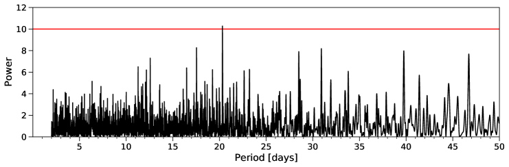
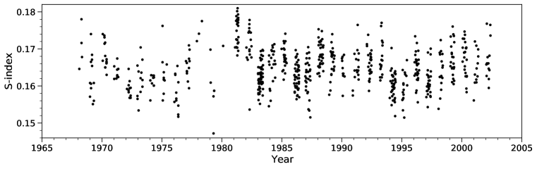
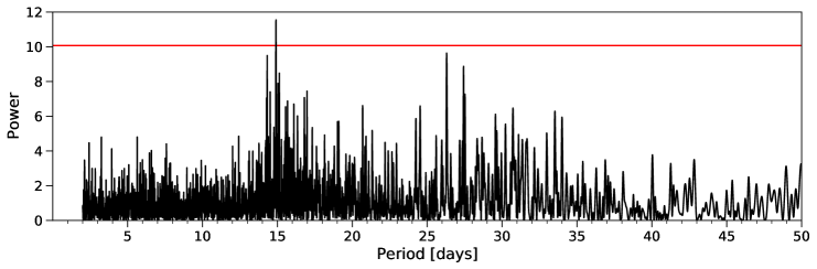
Figure 1: Time series and Lomb-Scargle periodograms for $\rho$ CrB (top two panels) and 88 Leo (bottom two panels) showing the recovered rotation signals of 20.3 days and 15.0 days, respectively. Red lines in the periodograms indicate the 5% false alarm probability calculated from a Monte Carlo process. (The data used to create this figure are available).

2 Observations

2.1 Mount Wilson HK data

Both $\rho$ CrB and 88 Leo have synoptic $S$-index time series from the MWO HK Project, ranging from near the beginning of the program in 1966 to its termination in 2003 (see Figure 1). The MWO $S$-index measures the ratio of emission from 1 Å cores of the Ca ii H & K lines to the sum of two nearby 20 Å pseudo-continuum bandpasses (Vaughan et al., 1978). Such measurements are routinely used in studies of magnetic activity cycles and stellar rotation (e.g. Baliunas et al., 1996; Donahue et al., 1996). Our analysis of the complete MWO time series gives a mean $S$-index of 0.1508 for $\rho$ CrB and 0.1655 for 88 Leo, in agreement with previous averages from the subset of data analyzed in Baliunas et al. (1995). Adopting the spectroscopic temperatures from Brewer et al. (2016) and the activity scale from Lorenzo-Oliveira et al. (2018), we find $\log R^{\prime}_{\rm HK}[T_{\rm eff}]=-5.177\pm 0.015$ for $\rho$ CrB and $-4.958\pm 0.015$ for 88 Leo (see Section 4).

We applied the Lomb-Scargle periodogram to the entire time series as well as seasonal bins in order to search for rotational signals. We took signals with a false alarm probability (FAP) less than 5% to be statistically significant. The FAP is defined as the probability that a peak in the periodogram is due to Gaussian noise (Horne & Baliunas, 1986), and we have calculated the FAP using that definition explicitly in a Monte Carlo simulation of 100,000 trials. In each trial, synthetic data of the same sampling cadence and standard deviation as the observational data are randomly drawn from the Gaussian distribution, and the Lomb-Scargle periodogram is computed. The fraction of random trials generating periodogram peaks higher than the one obtained from the observational data is the FAP. The uncertainty in the period is found by a similar Monte Carlo process where the observational data are moved within their 1% uncertainty (Baliunas et al., 1995) and the standard deviation of peak periods is computed. Using this method, we find a rotation period of $20.3\pm 1.8$ days for $\rho$ CrB (FAP = 4.2%) and $15.0\pm 0.3$ days for 88 Leo (FAP = 1.2%) from the complete time series. Figure 1 shows the time series and Lomb-Scargle periodograms for both stars, with the 5% FAP line computed from the Monte Carlo shown as a red line. Single season analyses returned no significant peaks for $\rho$ CrB (which is not unusual for “flat activity” stars, Donahue et al., 1996), and one season with a significant peak for 88 Leo, giving a rotation period of $14.3\pm 0.8$ days (FAP = 1.4%) and confirming the global result.

Our rotation period for $\rho$ CrB is $\sim$2$\sigma$ longer than the 17 days found by Baliunas et al. (1996), who used a subset of the MWO data and did not provide an uncertainty. However, our result agrees with Henry et al. (2000) who used a longer subset of the MWO data ($\langle P_{\rm rot}\rangle=19\pm 2$ days, with seasonal values between 17–20 days), and with Fulton et al. (2016) who found 18.5 days from Keck observations. For 88 Leo, we find good agreement with the 14 day rotation period determined by Baliunas et al. (1996) and the 14.32 day period determined by Oláh et al. (2009) from the complete MWO time series.

2.2 TESS photometry

TESS observed $\rho$ CrB in 2-minute cadence for a total of approximately 52 days during Sectors 24 and 25 of Cycle 2 (2020 Apr 15 – 2020 Jun 08). We downloaded the PDC-MAP SPOC light curve (Jenkins et al., 2016), but also derived our own light curve following the procedure described in Nielsen et al. (2020) and Buzasi et al. (2015) in hopes of improving on the noise level in the SPOC product. We treated sectors individually, masking cadences with nonzero quality flags. We then built a collection of single-pixel light curves for each pixel in the $25\times 25$ pixel postage stamp. Our figure of merit for the quality of a light curve was the sum of the absolute values of the first-differenced light curve, generally a good proxy for high-frequency noise (Nason, 2006). Starting from the brightest pixel, we then added pixels one at a time to the light curve, choosing in each case the pixel that produced the largest decrease in our noise figure of merit, and continuing until light curve quality no longer improved. This process resulted in a somewhat larger aperture than that derived by the SPOC (114 pixels vs. 59 for Sector 24 and 108 pixels vs. 51 for Sector 25). The resulting light curves were then detrended of instrumental effects by fitting a second-order polynomial in $x$ and $y$ pixel location. We compared the resulting light curve to the SPOC product; improvement was modest but noticeable ($\sim$6% decreased noise) at frequencies above 1 mHz, so we chose to use our light curve for the asteroseismic analysis in Section 3.1.

We applied a similar photometric reduction algorithm to 88 Leo. TESS observed this star in 2-minute cadence for a total of approximately 27 days during Sector 22 of Cycle 2 (2020 Feb 18 – 2020 Mar 18). Once again, the process resulted in a somewhat larger aperture than that derived by the TESS SPOC (71 pixels vs. 36). After extraction and detrending, the noise level was lowered by approximately 15% above 1 mHz.

2.3 Spectral Energy Distribution

In order to provide an initial, empirical constraint on the stellar luminosities and radii, we performed an analysis of the broadband spectral energy distributions (SEDs) together with the Gaia EDR3 parallaxes following the procedures described in Stassun & Torres (2016) and Stassun et al. (2017, 2018). We pulled the FUV and NUV fluxes from GALEX, the $UBV$ magnitudes from Mermilliod (2006), the Strömgren $uvby$ magnitudes from Paunzen (2015), the $JHK_{S}$ magnitudes from 2MASS, the W1–W4 magnitudes from WISE, and the $G\,G_{BP}\,G_{RP}$ magnitudes from Gaia. Together, the available photometry spans the full stellar SED over the wavelength range 0.2–22 $\mu$m (see Figure 2).

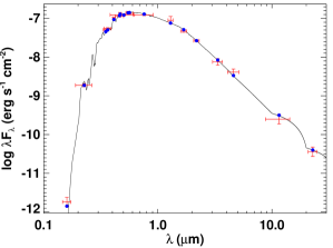
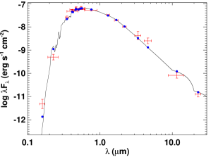
Figure 2: Spectral energy distributions for $\rho$ CrB (top) and 88 Leo (bottom). Red symbols are the observed photometric measurements, where the horizontal bars represent the effective width of the passband. Blue symbols are the model fluxes from the best-fit Kurucz atmosphere model (black).

We performed a fit using Kurucz stellar atmosphere models (Castelli & Kurucz, 2004), adopting the effective temperature ($T_{\rm eff}$) and metallicity ([M/H]) from the spectroscopically determined values of Brewer et al. (2016). Uncertainties were inflated to account for a realistic systematic noise floor: $T_{\rm eff}=5833\pm 78$ K, $\text{[M/H]}=-0.18\pm 0.07$ dex for $\rho$ CrB, and $T_{\rm eff}=6002\pm 78$ K, $\text{[M/H]}=+0.04\pm 0.07$ dex for 88 Leo. The extinction ($A_{V}$) was fixed at zero due to the proximity of the stars to Earth. The resulting fits (Figure 2) have a reduced $\chi^{2}$ between 1–2 for both stars. Integrating the (unreddened) model SED gives the bolometric flux at Earth ($F_{\rm bol}$). Taking this $F_{\rm bol}$ together with the Gaia EDR3 parallax, with no systematic adjustment (e.g., see Stassun & Torres, 2021), yields bolometric luminosities for $\rho$ CrB and 88 Leo of $L_{\rm bol}=1.746\pm 0.041\ L_{\odot}$ and $L_{\rm bol}=1.482\pm 0.088\ L_{\odot}$, respectively. In addition, the $L_{\rm bol}$ together with the $T_{\rm eff}$ yields stellar radii for $\rho$ CrB and 88 Leo of $R=1.295\pm 0.025\ R_{\odot}$ and $R=1.127\pm 0.037\ R_{\odot}$, respectively. Finally, we can estimate the stellar mass using the empirical eclipsing-binary based relations of Torres et al. (2010), which gives $M=1.09\pm 0.07\ M_{\odot}$ and $M=1.14\pm 0.07\ M_{\odot}$ for $\rho$ CrB and 88 Leo, respectively.

2.4 X-ray data

We obtained a Chandra observation of $\rho$ CrB using the High Resolution Camera imaging detector (HRC-I) on 2020 Apr 19 starting at UT 14:59 for a net exposure time of 11870 s. This instrument was chosen because it has the best available low-energy sensitivity for imaging observations. An earlier observation of $\rho$ CrB had also been obtained (PI: S. Saar) several years earlier on 2012 Jan 17 beginning at UT 13:12 using the Advanced CCD Imaging Spectrometer spectroscopic array (ACIS-S) on the back-illuminated CCD (“s3”) for a net exposure of 9835 s.

Both observations were downloaded from the Chandra archive and reprocessed using the Chandra Interactive Analysis of Observations (CIAO) software version 4.13 and calibration database version 4.9.4. While the ACIS-S data in principle have energy information for each photon from which a low-resolution X-ray spectrum can be derived, the $\rho$ CrB data contained only a handful of photon counts. The HRC-I data have no useful energy resolution. Analysis for both detectors therefore proceded similarly, by examining the photon counts attributable to $\rho$ CrB and using the instrument effective area to infer the implications for the X-ray flux. A summary of the observational results is presented in Table 1.

Table 1: Summary of Chandra results for $\rho$ CrB

Parameter	HRC-I	ACIS-S
Chandra ObsID	22308	12396
Net exposure (s)	11870	9835
$\rho$ CrB count rate (count ks-1)	$2.85\pm 0.51$	$0.77\pm 0.31$
Isothermal plasma temperature	$(1.58\pm 0.32)\times 10^{6}$ K
X-ray Luminosity $L_{X}^{a}$	$(9.1\pm 1.9)\times 10^{26}$ erg s-1

^aBest estimate of the X-ray luminosity assuming an isothermal optically-thin plasma radiative loss model with a solar mixture of abundances scaled by a metallicity [M/H] $=-0.18$, and an interstellar absorbing column of $1.95\times 10^{18}$ cm^-2.

In order to provide insight into the source X-ray luminosity giving rise to the HRC-I and ACIS-S signals, we used the PIMMS software version 4.11 to convert the observed HRC-I and ACIS-S count rates to the incident X-ray flux. Since we are lacking counts in the ACIS-S data to estimate a coronal temperature, we made the flux conversion for a range of isothermal plasma temperatures. We adopted the APEC optically-thin plasma radiative loss model (Foster et al., 2012), the metallicity of [M/H]=$-$0.18 from Brewer et al. (2016), and the solar abundance mixture of Asplund et al. (2009), together with an intervening hydrogen column density of $1.95\times 10^{18}$ cm^-2. This column density was estimated by interpolation within the compilations of column density measurements of Gudennavar et al. (2012) and Linsky et al. (2019), for the Gaia EDR3 distance of 17.51 pc.

The X-ray luminosities in the ROSAT 0.1–2.4 keV band corresponding to the observed HRC-I and ACIS-S count rates are illustrated as a function of isothermal plasma temperature in Figure 3. Shaded regions illustrate the range of uncertainties based on the uncertainties in the extracted count rates. Sensitivity of the results to the adopted absorbing column was determined by repeating the luminosity calculations for lower and higher values of $N_{\mathrm{H}}$ by a factor of two. Sensitivity to metallicity was also checked in a similar way, by varying metallicity by a factor of two, and found to be negligible.

Table 1 summarises the Chandra results for coronal luminosity and plasma temperature under the isothermal approximation. Final values were determined by the intersection of the HRC-I and ACIS-S $L_{X}$-$T$ loci and uncertainty ranges. By far the largest uncertainty is in the estimate of the X-ray count rates. The final estimate of the X-ray luminosity for $\rho$ CrB, $(9.1\pm 1.9)\times 10^{26}$ erg s^-1, is very similar to that of the quiet Sun (e.g. Judge et al., 2003), while the temperature is similar to the peak of the quiet Sun emission measure distribution (e.g. Brosius et al., 1996).

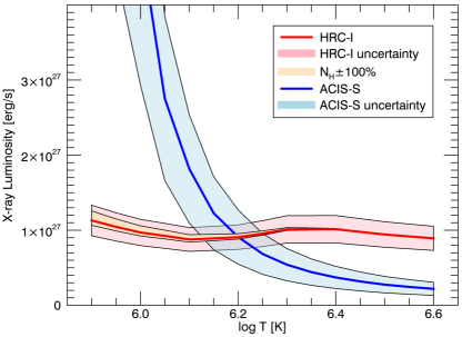
Figure 3: The X-ray luminosity of $\rho$ CrB for isothermal, collision-dominated, optically-thin plasma radiative loss as a function of plasma temperature implied by the observed Chandra HRC-I and ACIS-S count rates. Shaded regions indicate the uncertainties arising from the count rate measurements and a 100% error in the assessment of the intervening neutral hydrogen column density.

For 88 Leo, we start with the X-ray luminosity $\log L_{X}=27.77$ from Wright et al. (2011), which was derived from ROSAT PSPC data. This value was computed using the observed count rate ($0.0306\pm 0.0102$ counts s^-1, Voges et al., 2000) and the hardness ratio (HR = $-1$) calibration of Schmitt et al. (1995) with a distance of $d=23.0$ pc and $L_{\rm bol}=1.50\ L_{\odot}$. Adjusting for the updated properties from Section 2.3, we find $L_{X}\,=\,(6.1\pm 2.1)\times 10^{27}$ erg s^-1 and $\log L_{X}/L_{\rm bol}\,=\,-5.96^{+0.14}_{-0.19}$. Adopting the SED radius from Section 2.3, the surface flux is $\log F_{X}\,=\,4.90^{+0.14}_{-0.19}$. As a check, we used PIMMS with the above count rate, a column of $N_{H}\,=\,10^{18}$ cm^-2 (based on the star’s presence in the NGP cloud, Linsky et al., 2019), solar abundance and APEC models. We find $\log F_{X}\,=\,4.92$ at $T_{X}\,=\,1.04^{+0.75}_{-0.35}\times 10^{6}$ K, which is reasonable given the hardness ratio. The ROSAT observations were obtained in late 1990, when the Ca HK emission was slightly below the average level, so the X-ray observations should represent below average coronal conditions for 88 Leo.

3 Asteroseismology of $\rho$ CrB

3.1 Global oscillation parameters

The expected frequency of maximum power ($\nu_{\rm max}$) for $\rho$ CrB based on the TESS Asteroseismic Target List (ATL, Schofield et al., 2019) is $\approx$ 2000 $\mu$Hz, with a detection probability of $\approx$ 65%. The top panel of Figure 4 shows a power spectrum of the TESS light curve from Section 2.2. The spectrum displays a low signal-to-noise power excess around 1800 $\mu$Hz, which is consistent with the ATL given uncertainties in predicted $\nu_{\rm max}$ values.

To test whether the power excess is consistent with solar-like oscillations, we calculated an autocorrelation of the power spectrum between $\approx$ 1400-2100 $\mu$Hz (inset in the top panel of Figure 4). The autocorrelation shows a peak at $\approx$ 89 $\mu$Hz, close to the expected value for the characteristic large frequency separation ($\Delta\nu$) for solar-like oscillations in this frequency range (Stello et al., 2009). We furthermore calculated an échelle diagram (bottom panel of Figure 4) by dividing the power spectrum into equal segments with length $\Delta\nu$ and stacking one above the other, so that modes with a given spherical degree align vertically in ridges (Grec et al., 1983). The offset of the visible ridge in the échelle diagram, which is sensitive to the properties of the near-surface layers of the star (e.g. Christensen-Dalsgaard et al., 2014), is consistent with expectations for a ridge of dipole ($l=1$) modes based on Kepler measurements of stars with similar $\Delta\nu$ and $T_{\rm eff}$ (White et al., 2011).

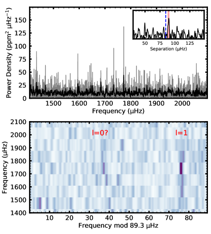
Figure 4: Top panel: Power density spectrum of the TESS light curve for $\rho$ CrB. The inset shows an autocorrelation of the power spectrum, with the expected large frequency separation marked by a vertical dashed line. The red shaded area marks the measured large separation. Bottom panel: Échelle diagram of the power spectrum in the top panel.

We used several independent methods (Huber et al., 2009; Mosser & Appourchaux, 2009; Mathur et al., 2010; Campante, 2018) to extract global oscillation parameters from the power spectrum, which yielded broadly consistent results. Estimates of $\nu_{\rm max}$ showed a large spread, as expected for a low signal-to-noise detection (Chaplin et al., 2014), so we did not adopt a constraint for our subsequent analysis. We adopted $\Delta\nu=89.3\pm 1.1\ \mu$Hz as measured by the SYD pipeline, which was consistent with measurements from other methods.

We also searched for oscillations in 88 Leo, which yielded a null detection. The star is not included in the ATL, but based on the stellar properties from Section 2 it is less evolved than $\rho$ CrB with an expected $\nu_{\rm max}$ of $\approx 2700$ $\mu$Hz and a detection probability $\approx$ 26%. Given the low S/N detection in $\rho$ CrB, the fainter apparent magnitude of 88 Leo, and the fact that oscillation amplitudes decrease with increasing $\nu_{\rm max}$ and with higher activity (García et al., 2010; Chaplin et al., 2011; Mathur et al., 2019), we conclude that the null detection is consistent with expectations.

3.2 Grid-based modeling

Grid-based modeling of $\rho$ CrB was performed using the Yale-Birmingham pipeline (Basu et al., 2010, 2012; Gai et al., 2011) with $\Delta\nu$, [M/H], $T_{\rm eff}$, and luminosity as inputs, and the results are listed in Table 3.2. The search was conducted on a grid containing two sub-grids—one with the solar-calibrated mixing length parameter, and the second using a metallicity-dependent mixing length, with the dependence given by Viani et al. (2018). Both sub-grids assume a linear relation $\Delta Y/\Delta Z\approx 1.5$ that was obtained using a calibrated solar model assuming a primordial helium abundance of $0.248$ (Steigman, 2010). The grids have models with masses between 0.7 $M_{\odot}$ and 3.3 $M_{\odot}$ in intervals of 0.025 $M_{\odot}$, evolved from the zero-age main-sequence to nearly the tip of the red-giant branch. The models were constructed with metallicities ranging from [M/H]=$-2.4$ to $+0.5$. The metallicity grid has a spacing of 0.1 dex between $-2.0$ and $+0.5$, and a spacing of 0.2 dex at lower metallicity. The metallicity scale is that of Grevesse & Sauval (1998), i.e., $\text{[M/H]}=0$ corresponds to $Z/X=0.023$.

The grids were constructed using the Yale Stellar Evolution Code (YREC, Demarque et al., 2008) for consistency with the rotational evolution modeling in Section 5. The models were constructed using OPAL opacities (Iglesias & Rogers, 1996) supplemented with low temperature opacities from Ferguson et al. (2005). The OPAL equation of state (Rogers & Nayfonov, 2002) was used. All nuclear reaction rates were obtained from Adelberger et al. (1998), except for that of the ${}^{14}N(p,\gamma)^{15}O$ reaction, for which we adopted the rate of Formicola et al. (2004). All models included gravitational settling of helium and heavy elements using the formulation of Thoul et al. (1994), with the diffusion coefficients smoothly decreased for stars more massive than $1.25\ M_{\odot}$. The large separation $\Delta\nu$ for the models were calculated from the frequencies of their radial modes, which in turn were calculated with the code of Antia & Basu (1994). The large separations were corrected for the surface term by applying the correction obtained by Viani et al. (2019).

Table 2: Stellar Properties of $\rho$ CrB and 88 Leo

	$\rho$ CrB
	Asteroseismic	Other		88 Leo	Source
$\log R^{\prime}_{\rm HK}[T_{\rm eff}]$ (dex)	$\cdots$	$-5.177\pm 0.015$		$-4.958\pm 0.015$	(1)
$P_{\rm rot}$ (days)	$\cdots$	$20.3\pm 1.8$		$15.0\pm 0.3$	(1)
$T_{\rm eff}$ (K)	$5817^{+32}_{-33}$	$5833\pm 78$		$6002\pm 78$	(2)
$[$M/H$]$ (dex)	$-0.19\pm 0.06$	$-0.18\pm 0.07$		$+0.04\pm 0.07$	(2)
$\log g$ (dex)	$4.190\pm 0.008$	$4.29\pm 0.08$		$4.38\pm 0.08$	(2)
Radius ($R_{\odot}$)	$1.304\pm 0.012$	$1.295\pm 0.025$		$1.127\pm 0.037$	(3)
Luminosity ($L_{\odot}$)	$1.749^{+0.036}_{-0.040}$	$1.746\pm 0.041$		$1.482\pm 0.088$	(3)
Mass ($M_{\odot}$)	$0.96\pm 0.02$	$1.09\pm 0.07$		$1.14\pm 0.07$	(3)
Age (Gyr)	$9.8^{+0.7}_{-0.5}$	$3.5\pm 0.6$		$2.4\pm 0.4$	(4)
$L_{X}$ ($10^{27}$ erg s-1)	$\cdots$	$0.91\pm 0.19$		$6.1\pm 2.1$	(5)

References. — (1) § 2.1; (2) Brewer et al. (2016); (3) § 2.3; (4) Barnes (2007); (5) § 2.4

4 Magnetic Evolution

4.1 Activity-age relation

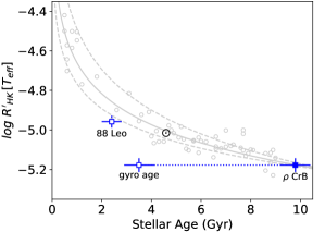
Figure 5: Chromospheric activity versus stellar age for a sample of spectroscopic solar twins from Lorenzo-Oliveira et al. (2018) with ages determined from isochrone fitting (gray circles). The asteroseismic age of $\rho$ CrB from TESS is overplotted as a solid square, while updated ages from gyrochronology for both stars are shown with open squares.

Considering the stellar properties determined above, we can now evaluate how the age expected from the chromospheric activity level compares to other age indicators. To facilitate this comparison, in Figure 5 we show the activity-age relation for a sample of spectroscopic solar twins from Lorenzo-Oliveira et al. (2018). The ages for this sample (gray circles) were determined from isochrone fitting, and the chromospheric activity scale was calibrated using $T_{\rm eff}$ rather than B$-$V color. The derived activity-age relation with uncertainties (gray lines) should be applicable to stars that have a mass and metallicity similar to the Sun. We can place other stars on this same activity scale using their spectroscopic $T_{\rm eff}$ and average $S$-index, with a small correction for non-solar metallicity (0.213$\times$[M/H], Saar & Testa, 2012). The horizontal error bars indicate the age uncertainty, while the vertical error bars reflect the uncertainties in $T_{\rm eff}$ and [M/H].

Using these procedures to place $\rho$ CrB and 88 Leo on the chromospheric activity scale for solar twins, we can evaluate their ages from asteroseismology and gyrochronology. The asteroseismic age for $\rho$ CrB from Table 3.2 is shown as a solid square in Figure 5, which falls directly on the activity-age relation for solar twins. Although we were unable to determine an asteroseismic age for 88 Leo, the age from gyrochronology should be reliable for this star because it is not yet below the critical activity level where weakened magnetic braking is inferred (van Saders et al., 2016; Brandenburg et al., 2017). The updated gyrochronology ages for both stars are indicated with open squares (Barnes, 2007), showing a reasonable agreement for 88 Leo considering its higher mass ($M_{\rm iso}=1.10\ M_{\odot}$, Valenti & Fischer, 2005) but revealing a strong disagreement for $\rho$ CrB. In Section 5, we examine this tension in greater detail.

4.2 Magnetic Braking Torque

We can estimate the strength of magnetic braking for $\rho$ CrB and 88 Leo by combining the wind modeling prescription of Finley & Matt (2017, 2018) with the constraints on magnetic morphology from Metcalfe et al. (2019). Given the polar strengths of an axisymmetric dipole, quadrupole, and/or octupole magnetic field, along with the mass-loss rate, rotation period, stellar mass and radius, this prescription yields an estimate of the magnetic braking torque based on analytical fits to a set of detailed magnetohydrodynamic wind simulations. Although 88 Leo exhibits a nonaxisymmetric polarization profile, the amplitude of the signal can be reproduced with an axisymmetric dipole having a polar field strength $B_{\rm d}=-5$ G. For $\rho$ CrB, Metcalfe et al. (2019) cite upper limits on the polar field strength assuming a pure axisymmetric dipole ($|B_{\rm d}|\leq 0.7$ G) or quadrupole field ($|B_{\rm q}|\leq 2.4$ G), with the latter being larger due to geometric cancellation effects. An identical analysis of the same LBT data yields an upper limit on a pure axisymmetric octupole field of $|B_{\rm o}|\leq 19.6$ G. However, the LBT observations also showed that the disk-integrated line-of-sight magnetic field in $\rho$ CrB is about 64% as strong as in 88 Leo, which agrees well with the relative chromospheric activity levels listed in Table 3.2. Given the upper limit on the dipole component, the global field of $\rho$ CrB appears to be dominated by quadrupolar and higher-order components to account for its relative line-of-sight field and activity level.

Observationally, the mass-loss rate is one of the least certain quantities required by the wind modeling prescription. If we initially fix the mass-loss rate to the solar value for both stars ($\dot{M}_{\odot}=2\times 10^{-14}\ M_{\odot}/\text{yr}$) and adopt the stellar properties from Table 3.2, we find that the magnetic braking torque for $\rho$ CrB is $\lesssim$20% as strong as for 88 Leo. This estimate does not depend strongly on whether we adopt the asteroseismic or other estimates of radius and mass for $\rho$ CrB, so we adopt the asteroseismic properties for further analysis. The mass-loss rate generally decreases with stellar age, so we might expect it to be larger than the solar value at the updated gyrochronology age of 88 Leo (2.4 Gyr), and smaller by the asteroseismic age of $\rho$ CrB (9.8 Gyr).

If we adopt the scaling relation $\dot{M}\propto F_{X}^{0.77}$ from Wood et al. (2021) and calculate the X-ray fluxes from the luminosities in Section 2.4, the mass-loss rate changes from 2.0 $\dot{M}_{\odot}$ to 0.36 $\dot{M}_{\odot}$ between the ages of these two stars, and the magnetic braking torque for $\rho$ CrB becomes $\lesssim$8% as strong as for 88 Leo. We can estimate the relative contributions to this total reduction in magnetic braking torque by changing the parameters of the 88 Leo wind model one at a time to the values in the $\rho$ CrB model. The largest factor that contributes to the reduction in magnetic braking torque is the shift in morphology towards quadrupolar and higher-order fields ($-$67% from shifting the field from pure dipole to pure quadrupole), followed by the evolutionary change in mass-loss rate ($-$60%), with smaller contributions from the weaker magnetic field (up to $-$34% from changing the strength of a quadrupole field from 5 G to 2.4 G) and slower rotation ($-$26%). The slightly lower mass (+4%) and evolutionary change in the radius (+58%) actually increase the relative magnetic braking torque, masking some of the other effects.

5 Rotational Evolution

We modeled the rotational evolution of $\rho$ CrB using the methodology laid out in Metcalfe et al. (2020). We assumed solid body rotation, and used the rotevol (Somers et al., 2017) tracer code to track the angular momentum evolution as a function of time, given a set of YREC evolutionary tracks and interpolation tools in kiauhoku (Claytor et al., 2020). We used the same model grid as that in Metcalfe et al. (2020) and adopted the same braking law parameters, with minor changes that we describe here. We scaled the critical Rossby number, Ro_crit in terms of the solar value, since the van Saders et al. (2016) model grid and our current grid have slightly different solar calibrations due to differing input physics. We adopted Ro${}_{\rm crit}=0.92~{}\textrm{Ro}_{\odot}$ as estimated in van Saders et al. (2019). Second, although unimportant for the late time rotational evolution, we chose a constant specific angular momentum (cm² s^-1) of $\log{j_{spec}}=16.3$ dex at 10 Myr (Somers et al., 2017) as our initial condition.

We utilized the same Monte Carlo approach as in Metcalfe et al. (2020) in which the mass, initial metallicity, age, and mixing length are parameters of the model, with the asteroseismic radius and the spectroscopic surface [M/H] and $T_{\rm eff}$ as the observables. We adopted strict Gaussian priors on the mass ($0.96\pm 0.02~{}M_{\odot}$) and age ($9.8\pm 0.8$ Gyr) from the asteroseismic analysis, and a broader prior on the mixing length ($1.8\pm 0.3$). In both cases, the rotation period is a prediction of the model, rather than a parameter we use in the fit itself. We used 8 walkers, each running for 100,000 steps.

The standard spin-down model predicts a rotation period of $52\pm 5$ days for $\rho$ CrB, while the weakened braking model with Ro${}_{\rm crit}=0.92~{}\textrm{Ro}_{\odot}$ predicts a rotation period of $28\pm 2$ days. We show in Figure 6 the posteriors on the predicted rotation distributions for both the standard spin-down and weakened magnetic braking cases in comparison to the observed period: both models predict longer periods.

We verified that changing the initial angular momentum is insufficient to relieve the tension, as in Metcalfe et al. (2020). Similarly, allowing the model to deviate from purely solid body rotation is also unlikely to result in more rapid rotation: in both the Sun and asteroseismic samples the rotation with depth is consistent with a solid body (Deheuvels et al., 2020). The convection zone of $\rho$ CrB has not yet begun to deepen at its current position in the HR diagram, and it is unlikely to be dredging up higher angular momentum material from a differentially rotating interior, even if such radial shear exists. Furthermore, when the core and envelope are allowed to decouple rotationally (MacGregor & Brenner, 1991) the surface rotation rate tends to be slower than a solid body model, because wind-driven loss drains angular momentum from the smaller, decoupled reservoir of the convective envelope. This star is also still hot enough ($\sim$5800 K) that assumptions about the convective mixing length have a comparatively mild effect on the predicted period.

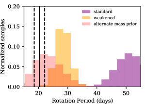
Figure 6: Predictions from a standard spin-down model (purple), weakened braking model (orange), and weakened braking model with a mass prior of $1.09\pm 0.07~{}M_{\odot}$ (pink) for the rotation period of $\rho$ CrB. The observed rotation period from Section 2.1 is shown with black vertical lines.

An underestimated stellar mass would result in predicted rotation periods that are too long, and indeed there is moderate tension between the asteroseismic mass and the empirical mass scale from eclipsing binaries. If we instead adopt a mass prior of $1.09\pm 0.07~{}M_{\odot}$ (while also adopting an uninformative age prior) we predict a period of $23^{+5}_{-4}$ days for the weakened magnetic braking case. The inferred mass is $1.00\pm 0.03\ M_{\odot}$ (consistent with the isochrone mass, Valenti & Fischer, 2005; Brewer et al., 2016), with predicted properties within 1$\sigma$ of the observed $L$, $R$, $T_{\rm eff}$, and surface [M/H]. The increased mass does require an age younger by about 2 Gyr (also consistent with isochrone estimates), but this is unsurprising: on the subgiant branch (SGB) near the turnoff, the age is tightly correlated with model mass. The ages of such stars are essentially equal to the main-sequence lifetime, and their rotational evolution shifts from being strongly dependent on time to strongly dependent on the structural evolution across the SGB.

We applied the same modeling techniques to 88 Leo, and find excellent agreement with the observed rotation period in both standard and weakened braking prescriptions. The predicted period is $15\pm 2$ days for both models: they do not differ significantly because the Rossby number of 88 Leo is approximately equal to our adopted critical Rossby number ($\textrm{Ro}=1.0\pm 0.1\ \textrm{Ro}_{\rm crit}$). Both the standard and weakened braking models are identical until the critical Rossby number is exceeded, and thus both predict the same rotation period for 88 Leo.

6 Summary and Discussion

By combining archival stellar activity data from MWO with asteroseismology from TESS, we have probed the nature of the transition that appears to decouple the evolution of rotation and magnetism in middle-aged stars. We characterized two stars ($\rho$ CrB and 88 Leo) with activity levels on opposite sides of the proposed mid-life transition—verifying their mean activity levels and rotation periods (Section 2.1), quantifying their X-ray luminosities to estimate mass-loss rates (Section 2.4), and deriving precise asteroseismic properties for the post-transition star $\rho$ CrB (Section 3). Analysis of the resulting observational constraints reveals that the asteroseismic age of $\rho$ CrB agrees with the expected evolution of its mean activity level, while the age from gyrochronology does not (Figure 5). No such tension exists for 88 Leo, suggesting a divergence in the evolution of rotation and magnetism between 2.4 and 3.5 Gyr for stars with shallower convection zones than the Sun.

Using a simple wind modeling prescription with previously published spectropolarimetric constraints on the global magnetic fields (Metcalfe et al., 2019), we find that the magnetic braking torque for $\rho$ CrB is more than an order of magnitude smaller than for 88 Leo, primarily due to a shift in morphology toward smaller spatial scales but reinforced by the evolutionary change in mass-loss rate and other properties (Section 4). Rotational evolution models adopting standard spin-down can match the observational constraints for 88 Leo, but they fail for $\rho$ CrB. By contrast, models with weakened magnetic braking can more readily explain the fast rotation of $\rho$ CrB, particularly if the asteroseismic properties are slightly biased from the relatively low S/N detection (Figure 6).

Future TESS observations may allow refinement of the stellar properties for $\rho$ CrB, and could yield an asteroseismic detection for 88 Leo. Both targets will be observed with 20-second cadence during Cycle 4, which yields a 20% longer effective integration time due to the absence of onboard cosmic ray rejection, and also avoids significant attenuation of signals near the Nyquist frequency of 2-minute sampling (Huber et al., 2021). The latter is particularly important for 88 Leo ($\nu_{\rm max}\approx 2700~{}\mu$Hz), which will be observed during Sectors 45-46 (2021 Nov/Dec) and Sector 49 (2022 Mar), further improving the detection probability. Although 88 Leo has a K-dwarf companion separated by 15$\farcs$5, it only dilutes the signal from the primary by $\sim$10%, and any solar-like oscillations in the K-dwarf are expected at a higher frequency and much lower amplitude. Additional observations of $\rho$ CrB will be obtained during Sector 51 (2022 May), and they can be combined with the Cycle 2 data to improve the S/N of the detection, potentially yielding a more precise value of $\Delta\nu$, a secure determination of $\nu_{\rm max}$, and perhaps some individual oscillation frequencies for detailed modeling. This may allow us to resolve the tension between the asteroseismic properties derived in Section 3 and the eclipsing binary mass scale, and possibly probe the impact of the observed non-solar abundance mixture for this star (Brewer et al., 2016).

Additional spectropolarimetic observations will provide new opportunities to test the mid-life transition hypothesis across a range of spectral types. Data recently obtained from the LBT include Stokes V measurements of 18 Sco, 16 Cyg A & B, $\lambda$ Ser, and HD 126053. The latter appears to be a transitional star like $\alpha$ Cen A (Metcalfe & van Saders, 2017), but with a rotation period and activity cycle very similar to the Sun. Such targets may offer the best constraints on the timescale for a shift in magnetic morphology, which must play out relatively quickly to explain the sudden reduction in magnetic braking torque suggested by observations (van Saders et al., 2016). By contrast, evolutionary changes in the mass-loss rate, mean activity level, and rotation period (as a star expands on the main-sequence) should take place more gradually. Aside from 18 Sco (which has a ground-based asteroseismic detection, Bazot et al., 2011), all of these targets will be observed by TESS with 20-second cadence in Cycle 4, and most of them have well-defined X-ray fluxes to constrain the mass-loss rates. Consequently, we should be able to extend the methodology applied above to a well-characterized sample of solar-type stars in the near future.

The authors would like to thank Steven Cranmer, B. J. Fulton, Sean Matt, Marc Pinsonneault, and Kaspar von Braun for helpful exchanges. T.S.M. acknowledges support from NSF grant AST-1812634, NASA grant 80NSSC20K0458, and Chandra award GO0-21005X. Computational time at the Texas Advanced Computing Center was provided through XSEDE allocation TG-AST090107. J.v.S. acknowledges support from NASA grant 80NSSC21K0246. D.B. acknowledges support from NASA through the Living With A Star Program (NNX16AB76G) and from the TESS GI Program under awards 80NSSC18K1585 and 80NSSC19K0385. J.J.D. was supported by NASA contract NAS8-03060 to the Chandra X-ray Center and thanks the Director, Pat Slane, for continuing advice and support. R.E. acknowledges NCAR for their support. The National Center for Atmospheric Research is sponsored by the National Science Foundation. D.H. acknowledges support from the Alfred P. Sloan Foundation, NASA grant 80NSSC21K0652, and NSF grant AST-1717000. S.H.S. is grateful for support from NASA Heliophysics LWS grant NNX16AB79G, and HST grant HST-GO-15991.002-A. W.H.B. acknowledges support from the UK Space Agency. T.L.C. is supported by Fundação para a Ciência e a Tecnologia (FCT) in the form of a work contract (CEECIND/00476/2018). A.J.F. is supported by the ERC Synergy grant “Whole Sun”, #810218. O.K. acknowledges support by the Swedish Research Council, the Royal Swedish Academy of Sciences, and the Swedish National Space Agency. S.M. acknowledges support from the Spanish Ministry of Science and Innovation with the Ramon y Cajal fellowship number RYC-2015-17697 and the grant number PID2019-107187GB-I00. T.R. acknowledges support from the European Research Council (ERC) under the European Union’s Horizon 2020 research and innovation program (grant agreement No. 715947). V.S. acknowledges funding from the European Research Council (ERC) under the European Union’s Horizon 2020 research and innovation program (grant agreement No. 682393 AWESoMeStars). This work benefited from discussions within the international team “The Solar and Stellar Wind Connection: Heating processes and angular momentum loss” at the International Space Science Institute (ISSI).

References

- Adelberger et al. (1998) Adelberger, E. G., Austin, S. M., Bahcall, J. N., et al. 1998, Reviews of Modern Physics, 70, 1265, doi: 10.1103/RevModPhys.70.1265
- Antia & Basu (1994) Antia, H. M., & Basu, S. 1994, A&AS, 107, 421
- Asplund et al. (2009) Asplund, M., Grevesse, N., Sauval, A. J., & Scott, P. 2009, ARA&A, 47, 481, doi: 10.1146/annurev.astro.46.060407.145222
- Baliunas et al. (1996) Baliunas, S., Sokoloff, D., & Soon, W. 1996, ApJ, 457, L99, doi: 10.1086/309891
- Baliunas et al. (1995) Baliunas, S. L., Donahue, R. A., Soon, W. H., et al. 1995, ApJ, 438, 269, doi: 10.1086/175072
- Barnes (2007) Barnes, S. A. 2007, ApJ, 669, 1167, doi: 10.1086/519295
- Basu et al. (2010) Basu, S., Chaplin, W. J., & Elsworth, Y. 2010, ApJ, 710, 1596, doi: 10.1088/0004-637X/710/2/1596
- Basu et al. (2012) Basu, S., Verner, G. A., Chaplin, W. J., & Elsworth, Y. 2012, ApJ, 746, 76, doi: 10.1088/0004-637X/746/1/76
- Bazot et al. (2011) Bazot, M., Ireland, M. J., Huber, D., et al. 2011, A&A, 526, L4, doi: 10.1051/0004-6361/201015679
- Benomar et al. (2018) Benomar, O., Bazot, M., Nielsen, M. B., et al. 2018, Science, 361, 1231, doi: 10.1126/science.aao6571
- Böhm-Vitense (2007) Böhm-Vitense, E. 2007, ApJ, 657, 486, doi: 10.1086/510482
- Brandenburg et al. (2017) Brandenburg, A., Mathur, S., & Metcalfe, T. S. 2017, ApJ, 845, 79, doi: 10.3847/1538-4357/aa7cfa
- Brewer et al. (2016) Brewer, J. M., Fischer, D. A., Valenti, J. A., & Piskunov, N. 2016, ApJS, 225, 32, doi: 10.3847/0067-0049/225/2/32
- Brosius et al. (1996) Brosius, J. W., Davila, J. M., Thomas, R. J., & Monsignori-Fossi, B. C. 1996, ApJS, 106, 143, doi: 10.1086/192332
- Buzasi et al. (2015) Buzasi, D. L., Carboneau, L., Hessler, C., Lezcano, A., & Preston, H. 2015, in IAU General Assembly, Vol. 29, 2256843
- Campante (2018) Campante, T. L. 2018, Asteroseismology and Exoplanets: Listening to the Stars and Searching for New Worlds, 49, 55, doi: 10.1007/978-3-319-59315-9_3
- Castelli & Kurucz (2004) Castelli, F., & Kurucz, R. L. 2004, A&A, 419, 725, doi: 10.1051/0004-6361:20040079
- Chaplin et al. (2014) Chaplin, W. J., Elsworth, Y., Davies, G. R., et al. 2014, MNRAS, 445, 946, doi: 10.1093/mnras/stu1811
- Chaplin et al. (2011) Chaplin, W. J., Bedding, T. R., Bonanno, A., et al. 2011, ApJ, 732, L5, doi: 10.1088/2041-8205/732/1/L5
- Christensen-Dalsgaard et al. (2014) Christensen-Dalsgaard, J., Silva Aguirre, V., Elsworth, Y., & Hekker, S. 2014, MNRAS, 445, 3685, doi: 10.1093/mnras/stu2007
- Claytor et al. (2020) Claytor, Z. R., van Saders, J. L., Santos, Â. R. G., et al. 2020, ApJ, 888, 43, doi: 10.3847/1538-4357/ab5c24
- Deheuvels et al. (2020) Deheuvels, S., Ballot, J., Eggenberger, P., et al. 2020, A&A, 641, A117, doi: 10.1051/0004-6361/202038578
- Demarque et al. (2008) Demarque, P., Guenther, D. B., Li, L. H., Mazumdar, A., & Straka, C. W. 2008, Ap&SS, 316, 31, doi: 10.1007/s10509-007-9698-y
- Donahue et al. (1996) Donahue, R. A., Saar, S. H., & Baliunas, S. L. 1996, ApJ, 466, 384, doi: 10.1086/177517
- Featherstone & Hindman (2016) Featherstone, N. A., & Hindman, B. W. 2016, ApJ, 830, L15, doi: 10.3847/2041-8205/830/1/L15
- Ferguson et al. (2005) Ferguson, J. W., Alexander, D. R., Allard, F., et al. 2005, ApJ, 623, 585, doi: 10.1086/428642
- Finley & Matt (2017) Finley, A. J., & Matt, S. P. 2017, ApJ, 845, 46, doi: 10.3847/1538-4357/aa7fb9
- Finley & Matt (2018) —. 2018, ApJ, 854, 78, doi: 10.3847/1538-4357/aaaab5
- Formicola et al. (2004) Formicola, A., Imbriani, G., Costantini, H., et al. 2004, Physics Letters B, 591, 61, doi: 10.1016/j.physletb.2004.03.092
- Foster et al. (2012) Foster, A. R., Ji, L., Smith, R. K., & Brickhouse, N. S. 2012, ApJ, 756, 128, doi: 10.1088/0004-637X/756/2/128
- Fruscione et al. (2006) Fruscione, A., McDowell, J. C., Allen, G. E., et al. 2006, in Society of Photo-Optical Instrumentation Engineers (SPIE) Conference Series, Vol. 6270, Society of Photo-Optical Instrumentation Engineers (SPIE) Conference Series, ed. D. R. Silva & R. E. Doxsey, 62701V, doi: 10.1117/12.671760
- Fulton et al. (2016) Fulton, B. J., Howard, A. W., Weiss, L. M., et al. 2016, ApJ, 830, 46, doi: 10.3847/0004-637X/830/1/46
- Gai et al. (2011) Gai, N., Basu, S., Chaplin, W. J., & Elsworth, Y. 2011, ApJ, 730, 63, doi: 10.1088/0004-637X/730/2/63
- García et al. (2010) García, R. A., Mathur, S., Salabert, D., et al. 2010, Science, 329, 1032, doi: 10.1126/science.1191064
- Garraffo et al. (2016) Garraffo, C., Drake, J. J., & Cohen, O. 2016, A&A, 595, A110, doi: 10.1051/0004-6361/201628367
- Garraffo et al. (2018) Garraffo, C., Drake, J. J., Dotter, A., et al. 2018, ApJ, 862, 90, doi: 10.3847/1538-4357/aace5d
- Grec et al. (1983) Grec, G., Fossat, E., & Pomerantz, M. A. 1983, Sol. Phys., 82, 55
- Grevesse & Sauval (1998) Grevesse, N., & Sauval, A. J. 1998, Space Sci. Rev., 85, 161, doi: 10.1023/A:1005161325181
- Gudennavar et al. (2012) Gudennavar, S. B., Bubbly, S. G., Preethi, K., & Murthy, J. 2012, ApJS, 199, 8, doi: 10.1088/0067-0049/199/1/8
- Hall et al. (2021) Hall, O. J., Davies, G. R., van Saders, J., et al. 2021, Nature Astronomy, doi: 10.1038/s41550-021-01335-x
- Henry et al. (2000) Henry, G. W., Baliunas, S. L., Donahue, R. A., Fekel, F. C., & Soon, W. 2000, ApJ, 531, 415, doi: 10.1086/308466
- Horne & Baliunas (1986) Horne, J. H., & Baliunas, S. L. 1986, ApJ, 302, 757, doi: 10.1086/164037
- Huber et al. (2009) Huber, D., Stello, D., Bedding, T. R., et al. 2009, Communications in Asteroseismology, 160, 74. https://arxiv.org/abs/0910.2764
- Huber et al. (2021) Huber, D., White, T. R., Metcalfe, T. S., & others. 2021, ApJ, submitted
- Iglesias & Rogers (1996) Iglesias, C. A., & Rogers, F. J. 1996, ApJ, 464, 943, doi: 10.1086/177381
- Jenkins et al. (2016) Jenkins, J. M., Twicken, J. D., McCauliff, S., et al. 2016, in Society of Photo-Optical Instrumentation Engineers (SPIE) Conference Series, Vol. 9913, Software and Cyberinfrastructure for Astronomy IV, ed. G. Chiozzi & J. C. Guzman, 99133E, doi: 10.1117/12.2233418
- Judge et al. (2003) Judge, P. G., Solomon, S. C., & Ayres, T. R. 2003, ApJ, 593, 534, doi: 10.1086/376405
- Linsky et al. (2019) Linsky, J. L., Redfield, S., & Tilipman, D. 2019, ApJ, 886, 41, doi: 10.3847/1538-4357/ab498a
- Lorenzo-Oliveira et al. (2018) Lorenzo-Oliveira, D., Freitas, F. C., Meléndez, J., et al. 2018, A&A, 619, A73, doi: 10.1051/0004-6361/201629294
- MacGregor & Brenner (1991) MacGregor, K. B., & Brenner, M. 1991, ApJ, 376, 204, doi: 10.1086/170269
- Mamajek & Hillenbrand (2008) Mamajek, E. E., & Hillenbrand, L. A. 2008, ApJ, 687, 1264, doi: 10.1086/591785
- Mathur et al. (2019) Mathur, S., García, R. A., Bugnet, L., et al. 2019, Frontiers in Astronomy and Space Sciences, 6, 46, doi: 10.3389/fspas.2019.00046
- Mathur et al. (2010) Mathur, S., García, R. A., Régulo, C., et al. 2010, A&A, 511, A46, doi: 10.1051/0004-6361/200913266
- Mermilliod (2006) Mermilliod, J. C. 2006, VizieR Online Data Catalog, II/168
- Metcalfe et al. (2016) Metcalfe, T. S., Egeland, R., & van Saders, J. 2016, ApJ, 826, L2, doi: 10.3847/2041-8205/826/1/L2
- Metcalfe et al. (2019) Metcalfe, T. S., Kochukhov, O., Ilyin, I. V., et al. 2019, ApJ, 887, L38, doi: 10.3847/2041-8213/ab5e48
- Metcalfe & van Saders (2017) Metcalfe, T. S., & van Saders, J. 2017, Sol. Phys., 292, 126, doi: 10.1007/s11207-017-1157-5
- Metcalfe et al. (2020) Metcalfe, T. S., van Saders, J. L., Basu, S., et al. 2020, ApJ, 900, 154, doi: 10.3847/1538-4357/aba963
- Mosser & Appourchaux (2009) Mosser, B., & Appourchaux, T. 2009, A&A, 508, 877, doi: 10.1051/0004-6361/200912944
- Mukai (1993) Mukai, K. 1993, Legacy, 3, 21
- Nason (2006) Nason, G. 2006, in Statistics in Volcanology, ed. H. Mader & S. Coles (United Kingdom: Geological Society of London), 129 – 142
- Nielsen et al. (2020) Nielsen, M. B., Ball, W. H., Standing, M. R., et al. 2020, A&A, 641, A25, doi: 10.1051/0004-6361/202037461
- Oláh et al. (2009) Oláh, K., Kolláth, Z., Granzer, T., et al. 2009, A&A, 501, 703, doi: 10.1051/0004-6361/200811304
- Paunzen (2015) Paunzen, E. 2015, A&A, 580, A23, doi: 10.1051/0004-6361/201526413
- Réville et al. (2015) Réville, V., Brun, A. S., Matt, S. P., Strugarek, A., & Pinto, R. F. 2015, ApJ, 798, 116, doi: 10.1088/0004-637X/798/2/116
- Ricker et al. (2014) Ricker, G. R., Winn, J. N., Vanderspek, R., et al. 2014, in Society of Photo-Optical Instrumentation Engineers (SPIE) Conference Series, Vol. 9143, Space Telescopes and Instrumentation 2014: Optical, Infrared, and Millimeter Wave, ed. J. Oschmann, Jacobus M., M. Clampin, G. G. Fazio, & H. A. MacEwen, 914320, doi: 10.1117/12.2063489
- Rogers & Nayfonov (2002) Rogers, F. J., & Nayfonov, A. 2002, ApJ, 576, 1064, doi: 10.1086/341894
- Saar & Testa (2012) Saar, S. H., & Testa, P. 2012, in Comparative Magnetic Minima: Characterizing Quiet Times in the Sun and Stars, ed. C. H. Mandrini & D. F. Webb, Vol. 286, 335–345, doi: 10.1017/S1743921312005066
- Schmitt et al. (1995) Schmitt, J. H. M. M., Fleming, T. A., & Giampapa, M. S. 1995, ApJ, 450, 392, doi: 10.1086/176149
- Schofield et al. (2019) Schofield, M., Chaplin, W. J., Huber, D., et al. 2019, The Astrophysical Journal Supplement Series, 241, 12, doi: 10.3847/1538-4365/ab04f5
- See et al. (2019) See, V., Matt, S. P., Finley, A. J., et al. 2019, ApJ, 886, 120, doi: 10.3847/1538-4357/ab46b2
- Skumanich (1972) Skumanich, A. 1972, ApJ, 171, 565, doi: 10.1086/151310
- Somers et al. (2017) Somers, G., Stauffer, J., Rebull, L., Cody, A. M., & Pinsonneault, M. 2017, ApJ, 850, 134, doi: 10.3847/1538-4357/aa93ed
- Stassun et al. (2017) Stassun, K. G., Collins, K. A., & Gaudi, B. S. 2017, AJ, 153, 136, doi: 10.3847/1538-3881/aa5df3
- Stassun et al. (2018) Stassun, K. G., Corsaro, E., Pepper, J. A., & Gaudi, B. S. 2018, AJ, 155, 22, doi: 10.3847/1538-3881/aa998a
- Stassun & Torres (2016) Stassun, K. G., & Torres, G. 2016, AJ, 152, 180, doi: 10.3847/0004-6256/152/6/180
- Stassun & Torres (2021) —. 2021, ApJ, 907, L33, doi: 10.3847/2041-8213/abdaad
- Steigman (2010) Steigman, G. 2010, J. Cosmology Astropart. Phys, 2010, 029, doi: 10.1088/1475-7516/2010/04/029
- Stello et al. (2009) Stello, D., Chaplin, W. J., Basu, S., Elsworth, Y., & Bedding, T. R. 2009, MNRAS, 400, L80, doi: 10.1111/j.1745-3933.2009.00767.x
- Strassmeier et al. (2015) Strassmeier, K. G., Ilyin, I., Järvinen, A., et al. 2015, Astronomische Nachrichten, 336, 324, doi: 10.1002/asna.201512172
- Thoul et al. (1994) Thoul, A. A., Bahcall, J. N., & Loeb, A. 1994, ApJ, 421, 828, doi: 10.1086/173695
- Torres et al. (2010) Torres, G., Andersen, J., & Giménez, A. 2010, A&A Rev., 18, 67, doi: 10.1007/s00159-009-0025-1
- Valenti & Fischer (2005) Valenti, J. A., & Fischer, D. A. 2005, ApJS, 159, 141, doi: 10.1086/430500
- van Saders et al. (2016) van Saders, J. L., Ceillier, T., Metcalfe, T. S., et al. 2016, Nature, 529, 181, doi: 10.1038/nature16168
- van Saders et al. (2019) van Saders, J. L., Pinsonneault, M. H., & Barbieri, M. 2019, ApJ, 872, 128, doi: 10.3847/1538-4357/aafafe
- Vaughan et al. (1978) Vaughan, A. H., Preston, G. W., & Wilson, O. C. 1978, PASP, 90, 267, doi: 10.1086/130324
- Viani et al. (2019) Viani, L. S., Basu, S., Corsaro, E., Ball, W. H., & Chaplin, W. J. 2019, ApJ, 879, 33, doi: 10.3847/1538-4357/ab232e
- Viani et al. (2018) Viani, L. S., Basu, S., Ong J., M. J., Bonaca, A., & Chaplin, W. J. 2018, ApJ, 858, 28, doi: 10.3847/1538-4357/aab7eb
- Voges et al. (2000) Voges, W., Aschenbach, B., Boller, T., et al. 2000, IAU Circ., 7432, 3
- White et al. (2011) White, T. R., Bedding, T. R., Stello, D., et al. 2011, ApJ, 743, 161, doi: 10.1088/0004-637X/743/2/161
- Wood (2018) Wood, B. E. 2018, in Journal of Physics Conference Series, Vol. 1100, Journal of Physics Conference Series, 012028, doi: 10.1088/1742-6596/1100/1/012028
- Wood et al. (2021) Wood, B. E., Mueller, H.-R., Redfield, S., et al. 2021, arXiv e-prints, arXiv:2105.00019. https://arxiv.org/abs/2105.00019
- Wright et al. (2011) Wright, N. J., Drake, J. J., Mamajek, E. E., & Henry, G. W. 2011, ApJ, 743, 48, doi: 10.1088/0004-637X/743/1/48