Dynamics of Colombo’s Top: Tidal Dissipation and Resonance Capture, With Applications to Oblique Super-Earths, Ultra-Short-Period Planets and Inspiraling Hot Jupiters

Abstract

We present a comprehensive theoretical study on the spin evolution of a planet under the combined effects of tidal dissipation and gravitational perturbation from an external companion. Such a “spin + companion” system (called Colombo’s top) appears in many [exo]planetary contexts. The competition between the tidal torque (which drives spin-orbit alignment and synchronization) and the gravitational torque from the companion (which drives orbital precession of the planet) gives rise to two possible spin equilibria (“Tidal Cassini Equilibria”, tCE) that are stable and attracting: the “simple” tCE1, which typically has a low spin obliquity, and the “resonant” tCE2, which can have a significant obliquity. The latter arises from a spin-orbit resonance and can be broken when the tidal alignment torque is stronger than the precessional torque from the companion. We characterize the long-term evolution of the planetary spin (both magnitude and obliquity) for an arbitrary initial spin orientation, and develop a new theoretical method to analytically obtain the probability of resonance capture driven by tidal dissipation. Applying our general theoretical results to exoplanetary systems, we find that a super-Earth (SE) with an exterior companion can have a substantial probability of being trapped in the high-obliquity tCE2, assuming that SEs have a wide range of primordial obliquities. We also evaluate the recently proposed “obliquity tide” scenarios for the formation of ultra-short-period Earth-mass planets and for the orbital decay of hot Jupiter WASP-12b. We find in both cases that the probability of resonant capture into tCE2 is generally low and that such a high-obliquity state can be easily broken by the required orbital decay.

1 Introduction

It is well recognized that the obliquity of a planet, the angle between the spin and orbital axes, likely reflects its dynamical history. In our Solar System, planetary obliquities (hereafter just “obliquities”) range from $3.1^{\circ}$ for Jupiter to $26.7^{\circ}$ for Saturn to $98^{\circ}$ for Uranus. The obliquities of exoplanets are challenging to measure, and so far only loose constraints have been obtained for the obliquity of a faraway ($\gtrsim 50\;\mathrm{AU}$) planetary-mass companion (Bryan et al., 2020). Nevertheless, there are prospects for better constraints on exoplanetary obliquities in the coming years, such as using high-resolution spectroscopy to measure $v\sin i$ for planetary rotation (Snellen et al., 2014; Bryan et al., 2018) and using high-precision photometry to measure the asphericity of a planet (Seager & Hui, 2002). Substantial obliquities are of increasing theoretical interest for their proposed role in explaining peculiar thermal phase curves (see e.g. Adams et al., 2019; Ohno & Zhang, 2019), in enhancing tidal dissipation in hot Jupiters (Millholland & Laughlin, 2018) and super-Earths (Millholland & Laughlin, 2019), and in the formation of ultra-short-period planets (USPs; Millholland & Spalding, 2020).

While nonzero obliquities are sometimes attributed to one or many giant impacts/collisions (e.g. Safronov & Zvjagina, 1969; Benz et al., 1989; Korycansky et al., 1990; Dones & Tremaine, 1993; Morbidelli et al., 2012; Li & Lai, 2020; Li et al., 2021), some studies suggest that large planetary obliquities may be produced by spin-orbit resonances. In this scenario, a rotating planet is subjected to a gravitational torque from its host star, making its spin axis precess around its orbital (angular momentum) axis. At the same time, the orbital axis precesses around another fixed axis under the gravitational influence of other masses in the system, e.g. additional planets or a protoplanetary disk. When the two precession frequencies become comparable, a resonance can occur that excites the obliquity to large values. This model is known as “Colombo’s Top” after the seminal work of Colombo (1966), and subsequent works have investigated the rich dynamics of this system (Peale, 1969, 1974; Ward, 1975; Henrard & Murigande, 1987). Such resonances have been invoked to explain the obliquities of both the Solar System gas giants (Ward & Hamilton, 2004; Hamilton & Ward, 2004; Ward & Canup, 2006; Vokrouhlickỳ & Nesvornỳ, 2015; Saillenfest et al., 2020, 2021) and the ice giants (Rogoszinski & Hamilton, 2019).

In a previous paper (Su & Lai, 2020, hereafter Paper I), we presented a systematic and general investigation of the dynamics of Colombo’s Top when the two precession frequencies of the system evolve through a commensurability. We obtained a semi-analytic mapping between the (arbitrary) planetary spin orientation and the final obliquity after a resonance encounter. We applied our results to investigate the generation of exoplanetary obliquities via a dissipating protoplanetary disk. However, our model did not consider the effect of additional torques in the system. In particular, tidal dissipation in the planet can cause the planet’s spin frequency to approach its orbital frequency and drive the planet’s spin axis towards its orbital axis, complicating the evolution of Colombo’s Top (Fabrycky et al., 2007; Levrard et al., 2007; Peale, 2008). In this paper, we extend these previous works to present a comprehensive study on how tidal dissipation influences the equilibria (called “Cassini States”) of the system and drive its long-term evolution. Our new results (summarized in Section 6) include a stability analysis of tide-modified Cassini States and a novel, analytic description/calculation of the resonance encounter process. We apply our general theoretical results to assess how obliquity tides may affect different types of exoplanetary systems.

Our paper is organized as follows. In Section 2, we briefly review the basic setup and non-dissipative dynamics of Colombo’s Top. In Section 3, we investigate the effect of adding a simple alignment torque to Colombo’s Top. The resulting dynamics captures the essential behavior that emerges due to tidal dissipation. In Section 4, we solve for the dynamics of the system including the full effect of tidal dissipation. In Section 5, we apply our results to three exoplanetary systems/scenarios of interest: (i) a super Earth with an exterior companion, (ii) the formation of USPs via obliquity tides, and (iii) the rapid orbital decay of the hot Jupiter WASP-12b. We summarize and discuss in Section 6.

2 Spin Evolution Equations and Cassini States: Review

In this section, we briefly review the spin dynamics of a planet in the presence of a distant perturber and introduce our notations; see Paper I for more details. We consider a star of mass $M_{\star}$ hosting an inner oblate planet of mass $m$ and radius $R$ on a circular orbit with semi-major axis $a$ and an outer perturber of mass $m_{\rm p}$ on a circular orbit with semi-major axis $a_{\rm p}$. The two orbits are mutually inclined by the angle $I$. Denote $\mathbf{S}$ the spin angular momentum and $\mathbf{L}$ the orbital angular momentum of the planet, and $\mathbf{L}_{\rm p}$ the angular momentum of the perturber. The corresponding unit vectors are $\hat{\boldsymbol{\mathbf{s}}}\equiv\mathbf{S}/S$, $\hat{\boldsymbol{\mathbf{l}}}\equiv\mathbf{L}/L$, and $\hat{\boldsymbol{\mathbf{l}}}_{\rm p}\equiv\mathbf{L}_{\rm p}/L_{\rm p}$. The spin axis $\hat{\boldsymbol{\mathbf{s}}}$ of the planet tends to precess around its orbital (angular momentum) axis $\hat{\boldsymbol{\mathbf{l}}}$, driven by the gravitational torque from the host star acting on the planet’s rotational bulge. On the other hand, $\hat{\boldsymbol{\mathbf{l}}}$ and $\hat{\boldsymbol{\mathbf{l}}}_{\rm p}$ precess around each other due to gravitational interactions. Assuming $S\ll L$, the equations of motion for $\hat{\boldsymbol{\mathbf{s}}}$ and $\hat{\boldsymbol{\mathbf{l}}}$ are

$$\frac{\mathrm{d}\hat{\boldsymbol{\mathbf{s}}}}{\mathrm{d}t} =\omega_{\rm sl}\left(\hat{\boldsymbol{\mathbf{s}}}\cdot\hat{\boldsymbol{\mathbf{l}}}\right)\left(\hat{\boldsymbol{\mathbf{s}}}\times\hat{\boldsymbol{\mathbf{l}}}\right)\equiv\alpha\left(\hat{\boldsymbol{\mathbf{s}}}\cdot\hat{\boldsymbol{\mathbf{l}}}\right)\left(\hat{\boldsymbol{\mathbf{s}}}\times\hat{\boldsymbol{\mathbf{l}}}\right),$$ (1)

$$\frac{\mathrm{d}\hat{\boldsymbol{\mathbf{l}}}}{\mathrm{d}t} =\omega_{\rm lp}\left(\hat{\boldsymbol{\mathbf{l}}}\cdot\hat{\boldsymbol{\mathbf{l}}}_{\rm p}\right)\left(\hat{\boldsymbol{\mathbf{l}}}\times\hat{\boldsymbol{\mathbf{l}}}_{\rm p}\right)\equiv-g\left(\hat{\boldsymbol{\mathbf{l}}}\times\hat{\boldsymbol{\mathbf{l}}}_{\rm p}\right),$$ (2)

where

$$\omega_{\rm sl} \equiv\alpha=\frac{3GJ_{2}mR^{2}M_{\star}}{2a^{3}\mathcal{I}\Omega_{\rm s}}=\frac{3k_{q}}{2k}\frac{M_{\star}}{m}\left(\frac{R}{a}\right)^{3}\Omega_{\rm s},$$ (3)

$$\omega_{\rm lp} \equiv-\frac{g}{\cos I}=\frac{3m_{\rm p}}{4M_{\star}}\left(\frac{a}{a_{\rm p}}\right)^{3}n.$$ (4)

In Eq. (3), $\Omega_{\rm s}$ is the spin frequency of the inner planet, $\mathcal{I}=kmR^{2}$ (with $k$ the normalized moment of inertia, often notated as $C_{\rm N}$) is its moment of inertia and $J_{2}=k_{\rm q}\Omega_{\rm s}^{2}(R^{3}/Gm)$ (with $k_{\rm q}$ a constant, related to the hydrostatic Love number $k_{2}$ by $k_{\rm q}=k_{2}/3$) is its rotation-induced (dimensionless) quadrupole moment [for a fluid body with uniform density, $k=0.4,k_{\rm q}=0.5$; for the Earth, $k\simeq 0.331$ and $k_{\rm q}\simeq 0.31$; for Jupiter, $k\simeq 0.27$ and $k_{\rm q}\simeq 0.18$ (e.g. Groten, 2004; Lainey, 2016)]. In other studies, $3k_{\rm q}/2k$ is often notated as $k_{2}/2C_{\rm N}$ (e.g. Millholland & Batygin, 2019). In Eq. (4), $n\equiv\sqrt{GM_{\star}/a^{3}}$ is the inner planet’s orbital mean motion, and we have assumed $a_{\rm p}\gg a$ and included only the leading-order (quadrupole) interaction between the inner planet and perturber (Section 5.2 discusses modifications to Eq. 4 when $a_{\rm p}\gtrsim a$). Eq. (2) neglects the back-reaction torque on $\hat{\boldsymbol{\mathbf{l}}}$ from $\hat{\boldsymbol{\mathbf{s}}}$; this is justified since $L\gg S$ (see Anderson & Lai, 2018 for the case when $L\sim S$). In Eq. (3) (and throughout Sections 2–4), we assume $L_{\rm p}\gg L$ so that $\hat{\boldsymbol{\mathbf{l}}}_{\rm p}$ is a constant (Section 5.3 discusses the case of $L\simeq L_{\rm p}$). Following the standard notations, we have defined $\alpha=\omega_{\rm sl}$ and $g\equiv-\omega_{\rm 1p}\cos I$ (e.g. Colombo, 1966).

As in Paper I, we combine Eqs. (1)–(2) into a single equation by transforming into a frame rotating about $\hat{\boldsymbol{\mathbf{l}}}_{\rm p}$ with frequency $g$. In this frame, $\hat{\boldsymbol{\mathbf{l}}}_{\rm p}$ and $\hat{\boldsymbol{\mathbf{l}}}$ are both fixed, and $\hat{\boldsymbol{\mathbf{s}}}$ evolves as

$$\left(\frac{\mathrm{d}\hat{\boldsymbol{\mathbf{s}}}}{\mathrm{d}t}\right)_{\rm rot}=\alpha\left(\hat{\boldsymbol{\mathbf{s}}}\cdot\hat{\boldsymbol{\mathbf{l}}}\right)\left(\hat{\boldsymbol{\mathbf{s}}}\times\hat{\boldsymbol{\mathbf{l}}}\right)+g\left(\hat{\boldsymbol{\mathbf{s}}}\times\hat{\boldsymbol{\mathbf{l}}}_{\rm p}\right).$$ (5)

We choose the coordinate system such that $\hat{\boldsymbol{\mathbf{z}}}=\hat{\boldsymbol{\mathbf{l}}}$ and $\hat{\boldsymbol{\mathbf{l}}}_{\rm p}$ lies in the $\hat{\boldsymbol{\mathbf{x}}}$-$\hat{\boldsymbol{\mathbf{z}}}$ plane. We describe $\hat{\boldsymbol{\mathbf{s}}}$ in spherical coordinates using the polar angle $\theta$, the planet’s obliquity, and $\phi$, the precessional phase of $\hat{\boldsymbol{\mathbf{s}}}$ about $\hat{\boldsymbol{\mathbf{l}}}$, defined so that when $\phi=0^{\circ}$, $\hat{\boldsymbol{\mathbf{l}}}_{\rm p}$ and $\hat{\boldsymbol{\mathbf{s}}}$ are on opposite sides of $\hat{\boldsymbol{\mathbf{l}}}$.

The equilibria of Eq. (5) are referred to as Cassini States (CSs; Colombo, 1966; Peale, 1969). We follow the notation of Paper I and introduce the parameter

$$\eta\equiv-\frac{g}{\alpha}=\frac{1}{2}\frac{k}{k_{\rm q}}\frac{m_{\rm p}m}{M_{\star}^{2}}\left(\frac{a}{a_{\rm p}}\right)^{3}\left(\frac{a}{R}\right)^{3}\frac{n}{\Omega_{\rm s}}\cos I.$$ (6)

For a given value of $\eta$, there can be either two or four CSs, all of which require $\hat{\boldsymbol{\mathbf{s}}}$ lie in the plane of $\hat{\boldsymbol{\mathbf{l}}}$ and $\hat{\boldsymbol{\mathbf{l}}}_{\rm p}$. In the standard nomenclature, CSs 1, 3, and 4 have $\theta<0$, implying that $\hat{\boldsymbol{\mathbf{s}}}$ and $\hat{\boldsymbol{\mathbf{l}}}_{\rm p}$ are on opposite sides of $\hat{\boldsymbol{\mathbf{l}}}$, while CS2 has $\theta>0$, implying that $\hat{\boldsymbol{\mathbf{s}}}$ and $\hat{\boldsymbol{\mathbf{l}}}$ are on the same side of $\hat{\boldsymbol{\mathbf{l}}}$. We depart from the standard convention and simply label the CSs using the polar angles $\theta$ and $\phi$ (with $\theta\in\left[0,\pi\right]$): Figure 1 shows the CS obliquities as a function of $\eta$. CS1 and CS4 do not exist when $\eta>\eta_{\rm c}$, where

$$\eta_{\rm c}\equiv\left(\sin^{2/3}\!I+\cos^{2/3}\!I\right)^{-3/2}.$$ (7)

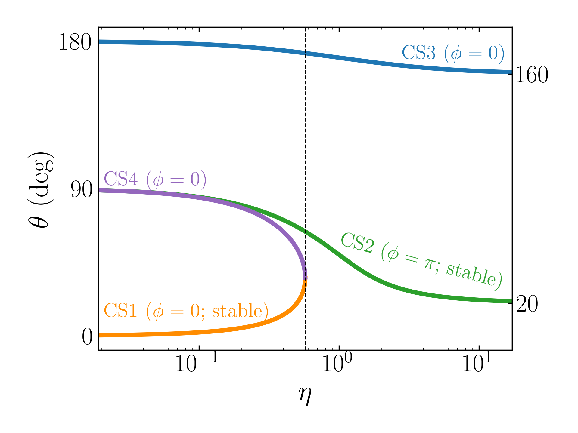
Figure 1: Cassini State obliquities $\theta$ as a function of $\eta\equiv-g/\alpha$ (Eq. 6) for $I=20^{\circ}$. The vertical dashed line denotes $\eta_{\rm c}$, where the number of Cassini States changes from four to two (Eq. 7). The y-axis labels on the right of the plot show the asymptotic obliquities for CS2 and CS3, $I$ and $180^{\circ}-I$ respectively. Note that $\theta$ does not follow the standard convention (e.g. Colombo, 1966, Paper I) and is simply the angle between $\hat{\boldsymbol{\mathbf{s}}}$ and $\hat{\boldsymbol{\mathbf{l}}}$, while $\phi=0$ corresponds to $\hat{\boldsymbol{\mathbf{s}}}$ and $\hat{\boldsymbol{\mathbf{l}}}_{\rm p}$ being on opposite sides of $\hat{\boldsymbol{\mathbf{l}}}$. While CSs 1–3 are “dynamically” stable, only CS1 and CS2 are stable and attracting in the presence of the spin-orbit alignment torque (see Section 3.2).

The Hamiltonian corresponding to Eq. (5) is

$$H =-\frac{\alpha}{2}\left(\hat{\boldsymbol{\mathbf{s}}}\cdot\hat{\boldsymbol{\mathbf{l}}}\right)^{2}-g\left(\hat{\boldsymbol{\mathbf{s}}}\cdot\hat{\boldsymbol{\mathbf{l}}}_{\rm p}\right)$$

$$=-\frac{\alpha}{2}\cos^{2}\theta-g\left(\cos\theta\cos I-\sin I\sin\theta\cos\phi\right).$$ (8)

Here, $\cos\theta$ and $\phi$ form a canonically conjugate pair of variables. Figure 2 shows the level curves of this Hamiltonian for $I=20^{\circ}$, for which $\eta_{\rm c}\approx 0.574$ (Eq. 7). When $\eta<\eta_{\rm c}$, CS4 exists and is a saddle point. The infinite-period orbits originating and ending at CS4 form the separatrix and divide phase space into three zones. The angle $\phi$ librates for trajectories in zone II and circulates for trajectories in zones I and III. On the other hand, when $\eta>\eta_{\rm c}$, the separatrix is absent and all trajectories circulate. When the separatrix exists, we divide it into two curves: $\mathcal{C}_{+}$, the boundary between zones I and II, and $\mathcal{C}_{-}$, the boundary between zones II and III.

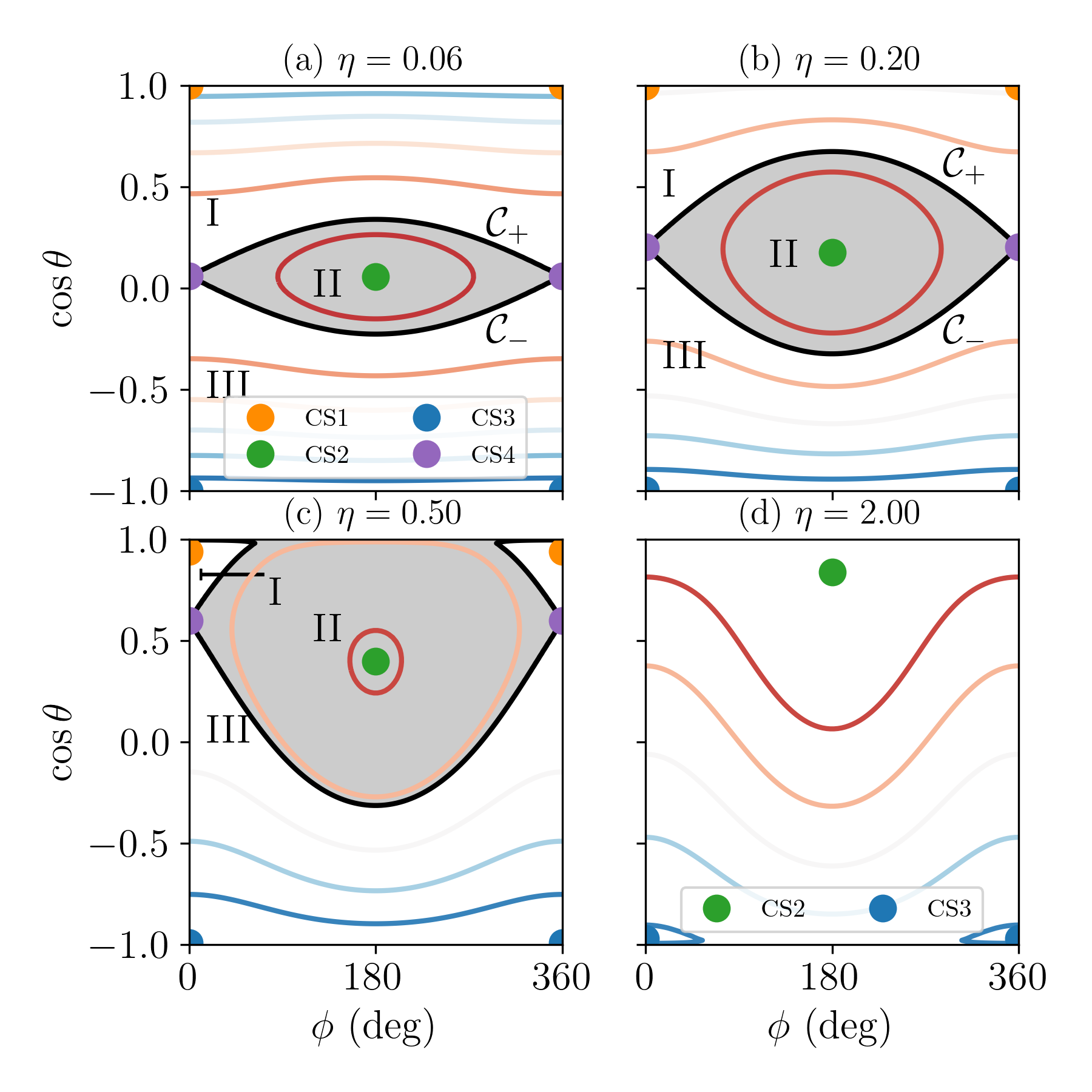
Figure 2: Level curves of the Hamiltonian (Eq. 8) for $I=20^{\circ}$, for which $\eta_{\rm c}\approx 0.57$ (Eq. 7). For $\eta<\eta_{\rm c}$, there are four Cassini States (labeled), while for $\eta>\eta_{\rm c}$ there are only two. In the former case, the existence of a separatrix (solid black lines) separates phase space into three numbered zones (I/II/III, labeled). We denote the upper and lower legs of the separatrix by $\mathcal{C}_{\pm}$ respectively, as shown in the upper two panels.

3 Spin Evolution with Alignment Torque

In this section, we consider a simplified dissipative torque that isolates the important new phenomenon presented in this paper. We assume that the spin magnitude of the planet is constant, so $\alpha$ and $g$ are both fixed, while the spin orientation $\hat{\boldsymbol{\mathbf{s}}}$ experiences an alignment torque towards $\hat{\boldsymbol{\mathbf{l}}}$ on the alignment timescale $t_{\rm al}$:

$$\left(\frac{\mathrm{d}\hat{\boldsymbol{\mathbf{s}}}}{\mathrm{d}t}\right)_{\rm tide}=\frac{1}{t_{\rm al}}\hat{\boldsymbol{\mathbf{s}}}\times\left(\hat{\boldsymbol{\mathbf{l}}}\times\hat{\boldsymbol{\mathbf{s}}}\right).$$ (9)

The full equations of motion for $\hat{\boldsymbol{\mathbf{s}}}$ in the coordinates $\theta$ and $\phi$ can be written as

$$\frac{\mathrm{d}\theta}{\mathrm{d}t} =-g\sin I\sin\phi-\frac{1}{t_{\rm al}}\sin\theta,$$ (10)

$$\frac{\mathrm{d}\phi}{\mathrm{d}t} =-\alpha\cos\theta-g\left(\cos I+\sin I\cot\theta\cos\phi\right).$$ (11)

3.1 Modified Cassini States

If the alignment torque is weak ($\left|g\right|t_{\rm al}\gg 1$), then the fixed points of Eqs. (10)–(11) are slightly modified CSs. To leading order, all of the CS obliquities $\theta_{\rm cs}$ are unchanged while the azimuthal angle $\phi_{\rm cs}$ for each CS now satisfies

$$\sin\phi_{\rm cs}=\frac{\sin\theta_{\rm cs}}{\sin I\left|g\right|t_{\rm al}}.$$ (12)

We can see that if $t_{\rm al}$ is longer than the critical alignment timescale $t_{\rm al,c}$, given for a particular $\theta_{\rm cs}$ by

$$t_{\rm al,c} \equiv\frac{\sin\theta_{\rm cs}}{\left|g\right|\sin I},$$ (13)

then Eq. (12) will always have solutions for $\phi_{\rm cs}$, and the alignment torque does not change the number of fixed points of the system. If $t_{\rm al}$ is decreased below $t_{\rm al,c}\sim\left|g\sin I\right|^{-1}$, CS2 and CS4 cease to be fixed points when $\eta\lesssim 1$ (as noted in Levrard et al., 2007; Fabrycky et al., 2007), as $\theta_{\rm cs}\sim 90^{\circ}$ for these (see Fig. 1). On the other hand, the other CSs have small $\sin\theta_{\rm cs}$ and are only slightly modified. Figure 3 shows the obliquity and azimuthal angle for each of the CSs when $\eta=0.2$, obtained via numerical root finding of Eqs. (10–11), where it can be seen that CS2 and CS4 collide and annihilate when $t_{\rm al}$ reaches $t_{\rm al,c}$. The phase shifts $\phi_{\rm cs}$ for CS2 and CS4 for $t_{\rm al}>t_{\rm al,c}$ can be predicted to good accuracy using Eq. (12) and $\theta_{\rm cs}\approx\pi/2-\eta\cos I\approx 79^{\circ}$ (Su & Lai, 2020); these are shown as the dashed lines in the bottom panel of Fig. 3. For the remainder of this section, we will consider the case where $t_{\rm al}\gg t_{\rm al,c}$ and the CSs only differ slightly from their unmodified locations.

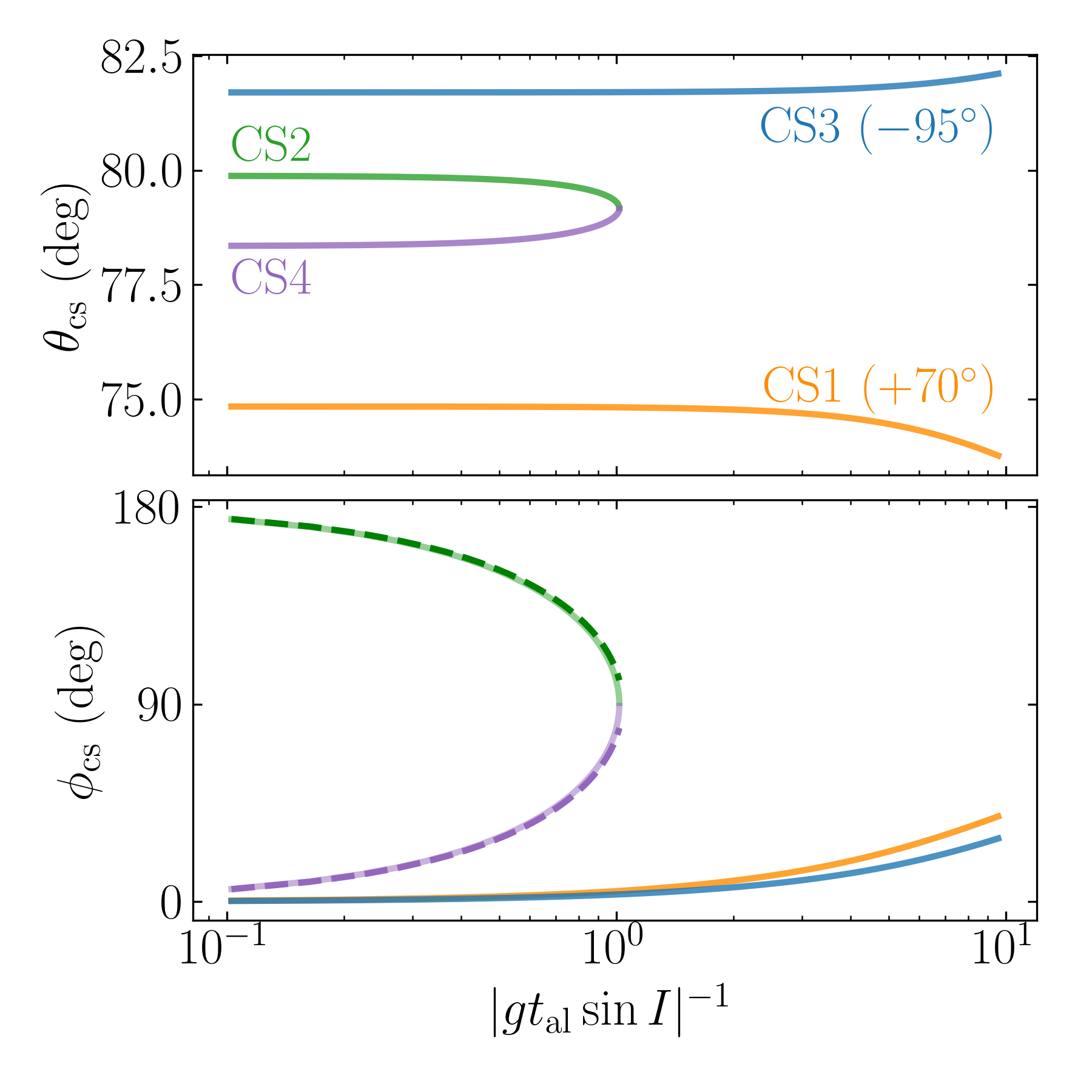
Figure 3: Modified CS obliquities (top) and azimuthal angles (bottom) for $I=20^{\circ}$ and $\eta=0.2$, where the CS1 and CS3 obliquities have been offset (as labeled) to improve clarity of the plot. In both panels, the solid lines give the result when applying a numerical root finding algorithm to the full equations of motion, Eqs. (10–11), while the dotted lines in the bottom panel give the CS2 and CS4 azimuthal angles according to Eq. (12). At $\left|gt_{\rm al}\sin I\right|=1$, CS2 and CS4 collide and annihilate (see Eq. 13).

3.2 Linear Stability Analysis

We next seek to characterize the stability of small perturbations about each of the CSs in the presence of the weak alignment torque. We can linearize Eqs. (10–11) about a shifted CS, yelding

$$\frac{\mathrm{d}}{\mathrm{d}t}\begin{bmatrix}\Delta\theta\\ \Delta\phi\end{bmatrix} =\begin{bmatrix}-\frac{\cos\theta}{t_{\rm al}}&-g\sin I\cos\phi\\ \alpha\sin\theta+g\frac{\sin I\cos\phi}{\sin^{2}\theta}&0\end{bmatrix}_{\rm cs}\begin{bmatrix}\Delta\theta\\ \Delta\phi\end{bmatrix},$$ (14)

where the “cs” subscript indicates evaluating at a CS, $\Delta\theta=\theta-\theta_{\rm cs}$, and $\Delta\phi=\phi-\phi_{\rm cs}$. The eigenvalues $\lambda$ of Eq. (14) satisfy the equation

$$0=\left(\lambda+\frac{\cos\theta_{\rm cs}}{t_{\rm al}}\right)\lambda-\lambda_{0}^{2},$$ (15)

where

$$\lambda_{0}^{2}\equiv\left(\alpha\sin\theta_{\rm cs}+g\sin I\csc^{2}\theta_{\rm cs}\cos\phi_{\rm cs}\right)\left(-g\sin I\cos\phi_{\rm cs}\right).$$ (16)

When $t_{\rm al}$ is large, we can simplify Eq. (15) to

$$\lambda\approx-\frac{\cos\theta_{\rm cs}}{t_{\rm al}}\pm\sqrt{\lambda_{0}^{2}}.$$ (17)

The stability of a CS depends on the real part of $\lambda$ in Eq. (17). Equation (17) $\lambda_{0}^{2}$ is a generalization of Eq. (A4) in Paper I and generally has the same behavior: it is negative for CSs 1–3 and positive for CS4, as shown in Fig. 4. Thus, CS4 is always “dynamically” unstable (i.e. unstable even in the limit of $t_{\rm al}\to\infty$), as there will always be at least one positive solution for $\lambda$. On the other hand, CSs 1–3 are dynamically stable, and their overall stabilities in the presence of the alignment torque are determined by the sign of $\cos\theta_{\rm cs}$. Using Fig. 1, we conclude that CS1 and CS2 are stable and attracting while trajectories near CS3 are driven away by the alignment torque. These calculations quantify the results long used in the literature (e.g. Ward, 1975; Fabrycky et al., 2007).

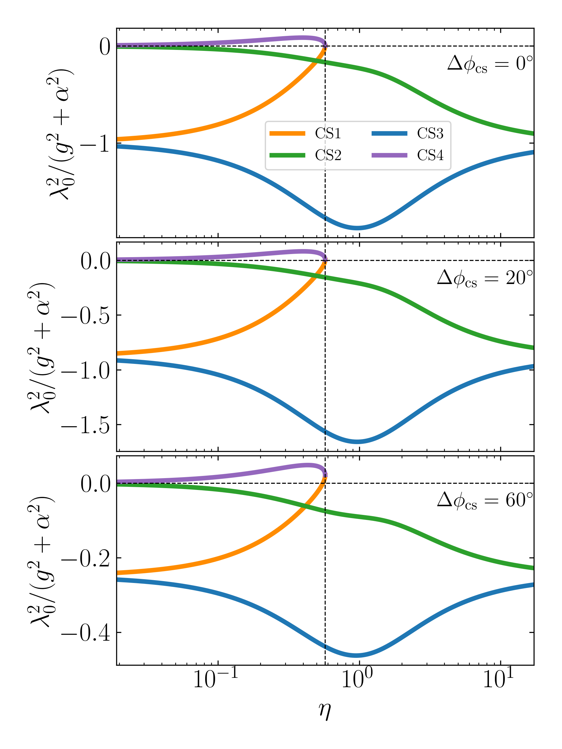
Figure 4: $\lambda_{0}^{2}$ (Eq. 16) as a function of $\eta$ for the four CSs, for three different values of the shift in $\phi_{\rm cs}$ (e.g. for $\Delta\phi_{\rm cs}=60^{\circ}$, the phase angles are $\phi_{\rm cs}=120^{\circ}$ for CS2 and $\phi_{\rm cs}=60^{\circ}$ for CSs 1, 3, and 4). The values of $\Delta\phi_{\rm cs}$ are labeled ($\Delta\phi_{\rm cs}=0$ corresponds to the unmodified CSs).

3.3 Spin Obliquity Evolution Driven by Alignment Torque

With the above results, we are equipped to ask questions about the dynamics of Eqs. (10–11): what is the long-term evolution of $\hat{\boldsymbol{\mathbf{s}}}$ for a general initial $\hat{\boldsymbol{\mathbf{s}}}_{\rm i}$?

For $\eta>\eta_{\rm c}$, the only stable (and attracting) spin state is CS2, and all initial conditions will evolve asymptotically towards it.

For $\eta<\eta_{\rm c}$, both CS1 and CS2 are stable (assuming the alignment torque is sufficiently weak that CS2 remains a fixed point; see Section 3.1), and spin evolution may involve separatrix crossing. To explore the fate of various initial $\hat{\boldsymbol{\mathbf{s}}}$ orientations, we numerically integrate Eqs. (10–11) for many random initial conditions uniformly distributed in $\left(\cos\theta_{\rm i},\phi_{\rm i}\right)$ and determine the nearest CS for each integration after $10t_{\rm al}$. In Fig. 5, we show the results of this procedure for $\eta=0.2$, and $I=20^{\circ}$ (we use $t_{\rm al}=10^{3}/\left|g\right|$, but the results are unchanged as long as $t_{\rm al}\gg\left|g\right|^{-1}$). It is clear that initial conditions in zone I evolve into CS1, those in zone II evolve into CS2, while those in zone III have a probabilistic outcome. These can be understood as follows:

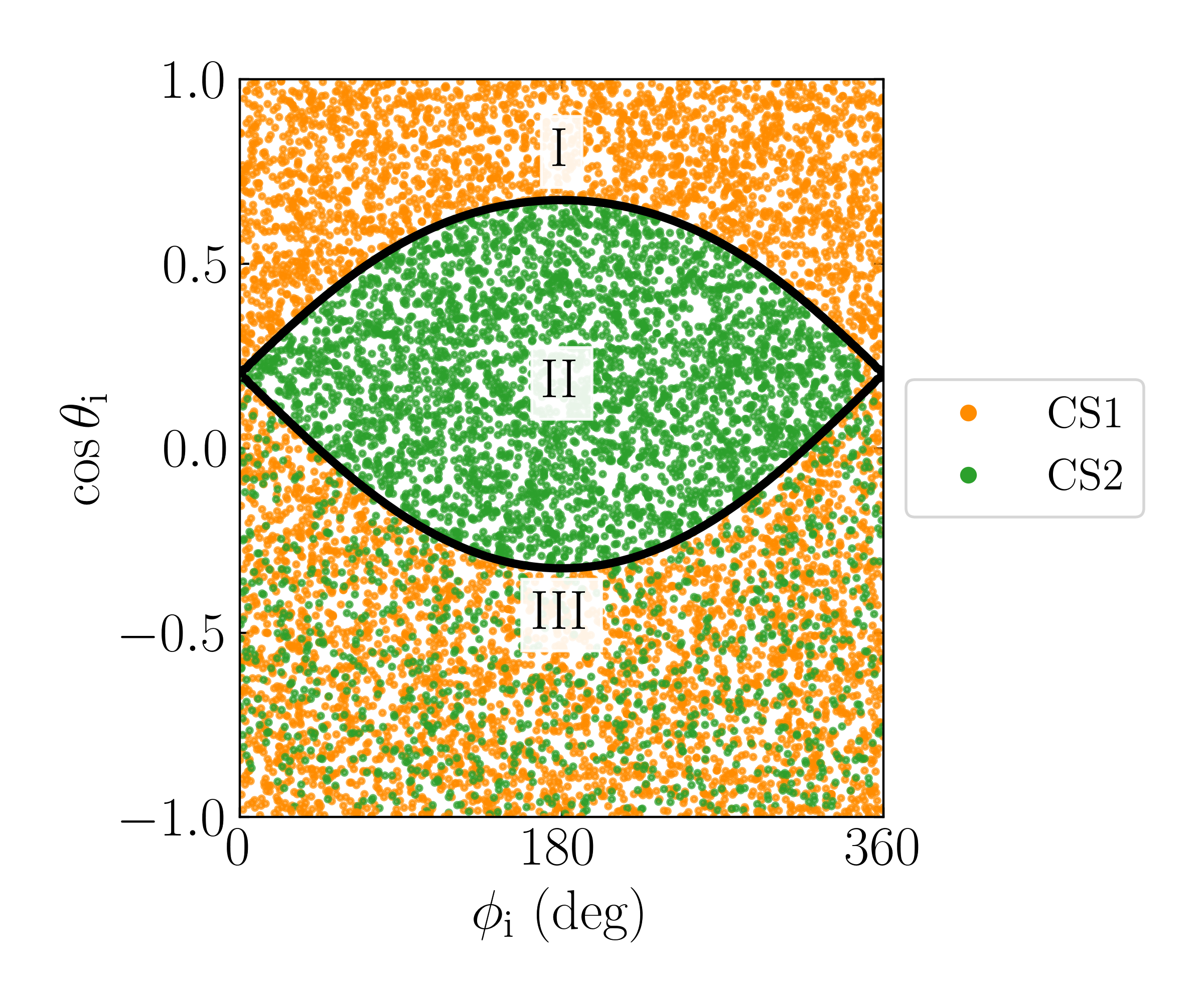
Figure 5: Asymptotic outcomes of spin evolution driven by an alignment torque for different initial spin orientations ($\theta_{\rm i}$ and $\phi_{\rm i}$) for a system with $\eta=0.2$ and $I=20^{\circ}$. Each dot represents an initial spin orientation, and the coloring of the dot indicates which stable Cassini State (legend) the system evolves into: initial conditions in Zone I evolve into CS1, those in Zone II evolve into CS2, and those in Zone III have a probabilistic outcome.

For initial conditions in zone I, the spin orientation circulates, and $\dot{\theta}$ is negative everywhere during the cycle. Thus $\theta$ decreases until the trajectory has converged to CS1. This is intuitively reasonable, as CS1 is stable and attracting (see Section 3.2).

For initial conditions in zone II, our stability analysis in Section 3.2 shows that when $\hat{\boldsymbol{\mathbf{s}}}$ is sufficiently near CS2, it will converge to CS2 since CS2 is stable and attracting. In fact, this result can be extended to all initial conditions inside the separatrix, as shown in Appendix A.

For initial conditions in zone III, since there are no stable CSs in zone III, the system must evolve through the separatrix to reach either CS1 or CS2. The outcome of the separatrix encounter is probabilistic and determines the final CS. Intuitively, this can be understood as probabilistic resonance capture, as first studied in the seminal work of Henrard (1982): for $\eta\lesssim\eta_{\rm c}\sim 1$, we have that $\alpha\gtrsim-g$, but $\alpha\cos\theta$ can become commensurate with $-g$ if $\cos\theta$ becomes small. This is achieved as $\theta$ evolves from an initially retrograde obliquity through $90^{\circ}$ towards $0^{\circ}$ under the influence of the alignment torque.

While similar in behavior to previous studies of probabilistic resonance capture (Henrard, 1982; Su & Lai, 2020), the underlying mechanism is different: In these previous studies, the phase space structure itself evolves and causes the system to transition among different phase space zones; here in the problem at hand, a non-Hamiltonian, dissipative perturbation causes the system to transition among fixed phase space zones. In the following subsection, we present an analytic calculation to determine the probability distribution of outcomes upon separatrix encounter. Readers not interested in the technical details can simply examine the resulting Fig. 7.

3.4 Analytical Calculation of Resonance Capture Probability

Before discussing our quantitative calculation, we first present a graphical understanding of the separatrix encounter process. Figure 6 shows how the perturbative alignment torque generates the two outcomes upon separatrix encounter, i.e. the zone III to zone II and the zone III to zone I transition. The critical trajectories in Fig. 6 are calculated numerically by integrating from a point infinitesimally close to CS4 forward and backward in time. In the absence of the alignment torque, these trajectories would evolve along the separatrix, but in the presence of the alignment torque, they are perturbed slightly and cease to overlap. It can be seen in Fig. 6 that this splitting opens a path from zone III into both zones I and II: the coloring scheme indicates that the trajectories within the orange and green regions of phase space stay within their respective colored regions.

To understand this process more concretely, and to compute the associated probabilities of the two possible outcomes, we consider the evolution of the value of the unperturbed Hamiltonian (Eq. 8) as the spin evolves due to the alignment torque. A point in zone III evolves such that $H$ is increasing until $H\approx H_{\rm sep}$, where $H_{\rm sep}$ is the value of $H$ along the separatrix, given by

$$H_{\rm sep} \equiv H\left(\cos\theta_{\rm 4},\phi_{\rm 4}\right)$$

$$\approx g\sin I+\frac{g^{2}}{2\alpha}\cos^{2}I+\mathcal{O}\left(\eta^{2}\right),$$ (18)

where

$$\theta_{4}\simeq\pi/2-\eta\cos I$$ (19)

(see Section A.1 of Paper I) and $\phi_{4}=0$ are the coordinates of CS4. As the system evolves closer to the separatrix, the change in $H$ over each circulation cycle can be approximated by $\Delta H_{-}$, the change in $H$ along $\mathcal{C}_{-}$ (see Fig. 2). In general, we define the quantities $\Delta H_{\pm}$

$$\Delta H_{\pm}\equiv\oint\limits_{\mathcal{C}_{\pm}}\frac{\mathrm{d}H}{\mathrm{d}t}\;\mathrm{d}t.$$ (20)

Using

$$\frac{\mathrm{d}H}{\mathrm{d}t} =\frac{\partial H}{\partial(\cos\theta)}\frac{\mathrm{d}(\cos\theta)}{\mathrm{d}t}+\frac{\partial H}{\partial\phi}\frac{\mathrm{d}\phi}{\mathrm{d}t}$$

$$=\left(\frac{\mathrm{d}(\cos\theta)}{\mathrm{d}t}\right)_{\rm tide}\frac{\mathrm{d}\phi}{\mathrm{d}t}$$ (21)

and Eq. (10), we find

$$\Delta H_{\pm} =\mp\frac{1}{t_{\rm al}}\int\limits_{0}^{2\pi}\sin^{2}\theta\;\mathrm{d}\phi,$$ (22)

where $\theta=\theta\left(\phi\right)$ is evolved along $\mathcal{C}_{\pm}$. Thus, if we evaluate $H$ every time that a trajectory originating in zone III crosses $\phi=0$, we see that will initially be $<H_{\rm sep}$ and increase for each circulation cycle until the system encounters the separatrix. At the beginning of the separatrix-crossing orbit, the initial value of $H$, denoted by $H_{\rm i}$, must be greater than $H_{\rm sep}-\Delta H_{-}$ to encounter the separatrix on the current orbit. We thus require

$$H_{\rm i}\in\left[H_{\rm sep}-\Delta H_{-},H_{\rm sep}\right].$$ (23)

The values of $\cos\theta$ corresponding to the lower and upper bounds in this range are shown as the black and purple dots on the left of Fig. 6 respectively.

During the separatrix-crossing orbit, the trajectory first evolves approximately along $\mathcal{C}_{-}$ and then along $\mathcal{C}_{+}$, after which the final value of $H$, denoted by $H_{\rm f}$, is approximately equal to

$$H_{\rm f}=H_{\rm i}+\Delta H_{+}+\Delta H_{-}.$$ (24)

There are two outcomes depending on the value of $H_{\rm f}$:

• If $H_{\rm f}<H_{\rm sep}$, then, since $H<H_{\rm sep}$ corresponds to the exterior of the separatrix, this implies that the trajectory has ended outside of the separatrix. This outcome thus corresponds to a zone III to zone I transition. In Fig. 6, the evolution within the orange shaded regions exhibits such an outcome.

• If $H_{\rm f}>H_{\rm sep}$, then the trajectory has instead ended inside of the separatrix and has executed a zone III to zone II transition. This corresponds to evolution within the green shaded regions in Fig. 6.

These two possibilities can be re-expressed in terms of $H_{\rm i}$: if $H_{\rm i}$ is in the interval $\left[H_{\rm sep}-\Delta H_{-},H_{\rm sep}-\Delta H_{-}-\Delta H_{+}\right]$, then the system executes a III $\to$ I transition, and if it is in the interval $\left[H_{\rm sep}-\Delta H_{-}-\Delta H_{+},H_{\rm sep}\right]$, then the system executes a III $\to$ II transition. We see that there is a critical value of $H_{\rm i}$,

$$\left(H_{\rm i}\right)_{\rm crit}=H_{\rm sep}-\Delta H_{-}-\Delta H_{+},$$ (25)

that separates the two possible outcomes of the separatrix encounter within the interval given by Eq. (23). The value of $\cos\theta$ for which $H$ is equal to $H_{\rm sep}-\Delta H_{-}-\Delta H_{+}$ is shown as the blue dot on the left of Fig. 6. Finally, if the alignment torque is weak, then $\left|\Delta H_{\pm}\right|\propto t_{\rm al}^{-1}$ is small compared to any variation in the value of $H$ (e.g. when changing the initial $\phi_{\rm i}$ or $\theta_{\rm i}$ by a small amount), and $H_{\rm i}$ can be effectively considered as randomly chosen from a uniform distribution over the range $\left[H_{\rm sep}-\Delta H_{-},H_{\rm sep}\right]$. As a consequence we obtain the probability of the III $\to$ II transition:

$$P_{\rm III\to II}=\frac{\Delta H_{-}+\Delta H_{+}}{\Delta H_{-}}.$$ (26)

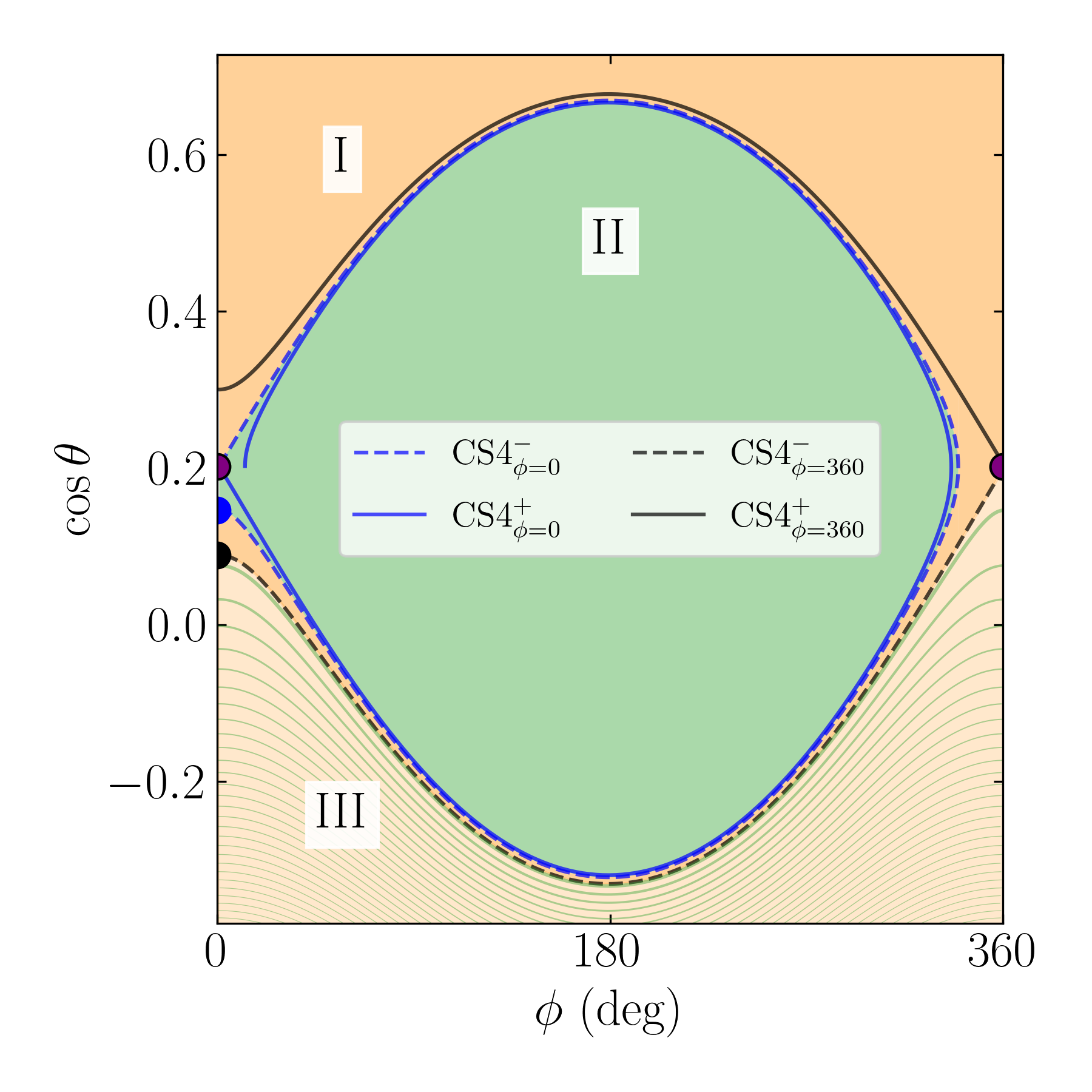
Figure 6: Plot illustrating the probabilistic origin of separatrix (resonance) capture for a system with $\eta=0.2$ and $I=20^{\circ}$. The orange regions converge to CS1, and the green to CS2. The purple dots denote CS4, a saddle point. The boundaries separating the CS1 and CS2-approaching regions consist of four critical trajectories (labeled in the legend) that are evolved starting from infinitesimal displacements from CS4 along its stable and unstable eigenvectors going forwards and backwards in time: e.g. the trajectory labeled CS4${}_{\phi=0}^{+}$ starts at $\phi=\epsilon$ (for some small, positive $\epsilon$) and evolves forwards in time (with $t_{\rm al}=10^{3}\left|g\right|^{-1}$), while the trajectory labeled CS4${}_{\phi=360}^{-}$ starts at $\phi=360^{\circ}-\epsilon$ and evolves backwards in time. The blue and black dots denote the intersections of CS4${}_{\phi=0}^{-}$ and CS4${}_{\phi=360}^{-}$ critical trajectories with the vertical line $\phi=0$. These critical trajectories can be used to understand the probabilistic outcomes that trajectories originating in zone III experience upon separatrix encounter, illustrated by the tightly spaced orange and green bands in zone III; see Section 3.4 for additional details.

To evaluate Eq. (26) analytically, we use the approximate expression for the separatrix $\eta\ll 1$ (see Eq. B5 of Paper I):

$$\left(\cos\theta\right)_{\mathcal{C}_{\pm}}\approx\eta\cos I\pm\sqrt{2\eta\sin I\left(1-\cos\phi\right)}.$$ (27)

Using Eq. (22), we find

$$\Delta H_{-} \approx\frac{2\pi}{t_{\rm al}}\left(1-2\eta\sin I\right)+\mathcal{O}(\eta^{3/2}),$$ (28)

$$\Delta H_{+}+\Delta H_{-} \approx\frac{32\eta^{3/2}\cos I\sqrt{\sin I}}{t_{\rm al}}+\mathcal{O}\left(\eta^{5/2}\right),$$ (29)

and thus

$$P_{\rm III\to II} \approx\frac{16\eta^{3/2}\cos I\sqrt{\sin I}}{\pi\left(1-2\eta\sin I\right)}.$$ (30)

To compare Eq. (30) with numerical results, we perform numerical integrations of Eqs. (10–11) while restricting the initial conditions to those in zone III. In Fig. 7, we display Eq. (30) alongside the computed $P_{\rm III\to II}$ using $1000$ initial conditions in zone III for each of $60$ values of $\eta$. Excellent agreement is observed.

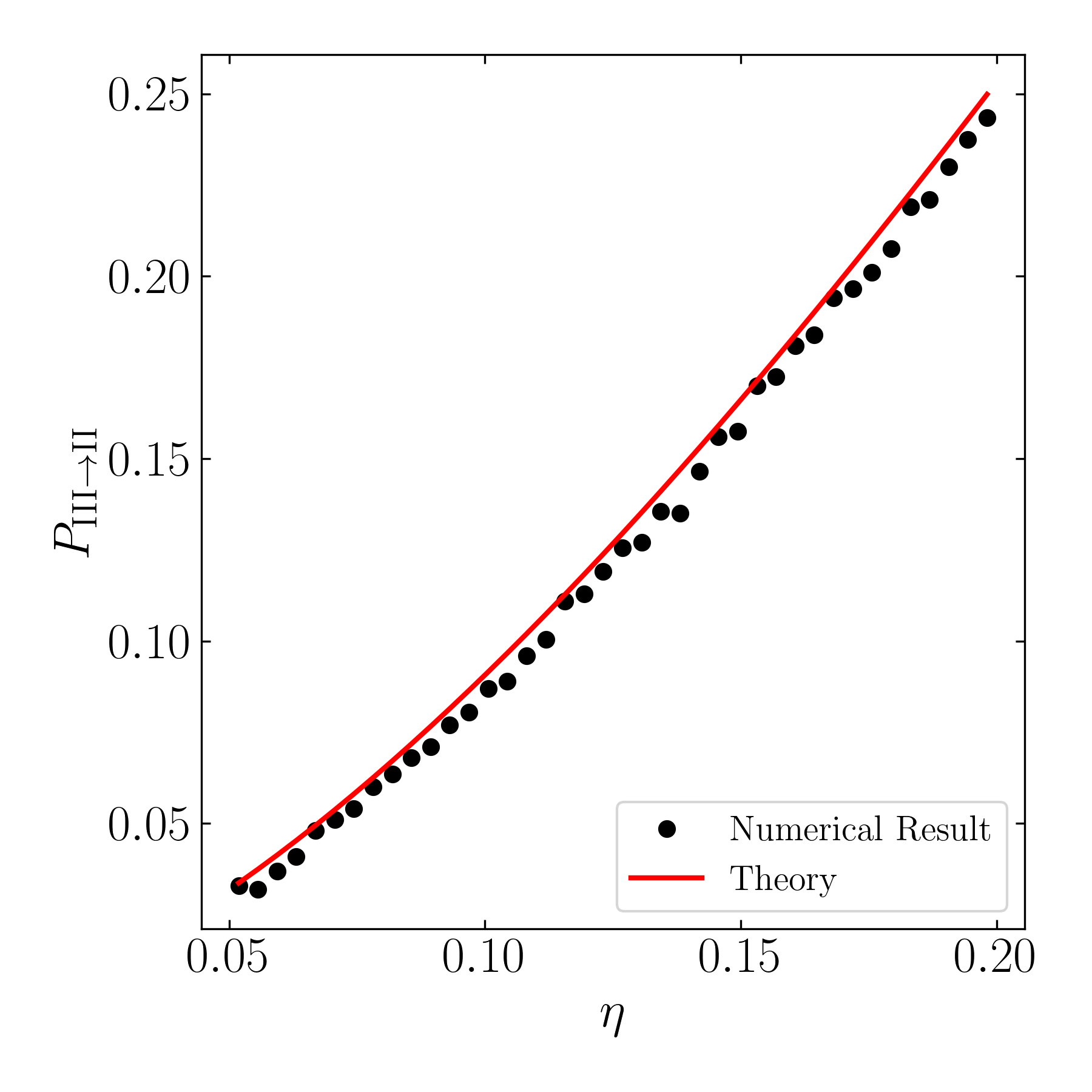
Figure 7: Zone III to Zone II transition probability $P_{\rm III\to II}$ upon separatrix encounter as a function of $\eta$ driven by an alignment torque. For each $\eta$, $1000$ initial random $\left(\theta_{\rm i},\phi_{\rm i}\right)$ values in zone III are evolved until just after separatrix encounter, where the outcome of the encounter is recorded. The red line shows the analytical result, Eq. (30).

The rigorous connection between the above calculation, focusing on the evolution of $H$ along the two legs of the separatrix $\mathcal{C}_{\pm}$, and the graphical picture illustrated in Fig. 6 is provided by Melnikov’s Method (Guckenheimer & Holmes, 1983). Melnikov’s Method is a general calculation that gives the degree of splitting of a “homoclinic orbit” (here, the separatrix) of a Hamiltonian system induced by a small, possibly time-dependent, perturbation. At a qualitative level, we can state the connection succinctly (see Fig. 6):

• The trajectory labeled CS4${}_{\phi=360}^{-}$ is evolved backwards in time from CS4 (where the Hamiltonian has the value $H_{\rm sep}$) along $\mathcal{C}_{-}$, and thus the black dot labels the start of a separatrix-crossing orbit with the initial value of the Hamiltonian $H_{\rm i}=H_{\rm sep}-H_{-}$. According to Eq. (23), this is exactly the minimum $H_{\rm i}$ such that a trajectory experiences a separatrix-crossing orbit. This is consistent with Fig. 6, where it is clear that any trajectories below the black dot at $\phi=0$ will not experience a separatrix encounter on its current circulation cycle.

• The trajectory labeled CS4${}_{\phi=0}^{-}$ is the one evolving backwards in time from CS4 along first $\mathcal{C}_{+}$ then $\mathcal{C}_{-}$, and thus the blue dot labels the start of a separatrix-crossing orbit with $H_{\rm i}=H_{\rm sep}-\Delta H_{-}-\Delta H_{+}$. According to Eq. (25), this is exactly the critical value of $H_{\rm i}$ that separates trajectories executing a III$\to$II transition and a III$\to$I transition. This is also consistent with Fig. 6, where the region above CS4${}_{\phi=0}^{-}$ is colored green while the region below is colored orange.

4 Spin Evolution with Weak Tidal Friction

4.1 Tidal Cassini Equilibria (tCE)

Having understood the effect of the alignment torque on the spin evolution (Section 3), we now implement the full effect of tidal dissipation, including both tidal alignment and spin synchronization. We use the weak friction theory of equilibrium tides (e.g. Alexander, 1973; Hut, 1981). In this model, tides cause both the spin orientation $\hat{\boldsymbol{\mathbf{s}}}$ and frequency $\Omega_{\rm s}$ to evolve on the characteristic tidal timescale $t_{\rm s}$ following (see Lai, 2012):

$$\left(\frac{\mathrm{d}\hat{\boldsymbol{\mathbf{s}}}}{\mathrm{d}t}\right)_{\rm tide} =\frac{1}{t_{\rm s}}\left[\frac{2n}{\Omega_{\rm s}}-\left(\hat{\boldsymbol{\mathbf{s}}}\cdot\hat{\boldsymbol{\mathbf{l}}}\right)\right]\hat{\boldsymbol{\mathbf{s}}}\times\left(\hat{\boldsymbol{\mathbf{l}}}\times\hat{\boldsymbol{\mathbf{s}}}\right),$$ (31)

$$\frac{1}{\Omega_{\rm s}}\left(\frac{\mathrm{d}\Omega_{\rm s}}{\mathrm{d}t}\right)_{\rm tide} =\frac{1}{t_{\rm s}}\left[\frac{2n}{\Omega_{\rm s}}\left(\hat{\boldsymbol{\mathbf{s}}}\cdot\hat{\boldsymbol{\mathbf{l}}}\right)-1-\left(\hat{\boldsymbol{\mathbf{s}}}\cdot\hat{\boldsymbol{\mathbf{l}}}\right)^{2}\right],$$ (32)

where $t_{\rm s}$ is given by

$$\frac{1}{t_{\rm s}}\equiv\frac{1}{4k}\frac{3k_{2}}{Q}\left(\frac{M_{\star}}{m}\right)\left(\frac{R}{a}\right)^{3}n,$$ (33)

with $k_{2}$ and $Q$ the tidal Love number and tidal quality factor, respectively. We neglect orbital evolution (thus, $t_{\rm s}$ is a constant) in this section since the time scale is longer than $t_{\rm s}$ by a factor of $\sim L/S\gg 1$ (we discuss the effect of orbital evolution in Section 5.3). We will continue to consider the case where tidal dissipation is slow, i.e. $\left|g\right|t_{\rm s}\gg 1$. The full equations of motion including weak tidal friction can be written in component form as

$$\frac{\mathrm{d}\theta}{\mathrm{d}t} =g\sin I\sin\phi-\frac{1}{t_{\rm s}}\sin\theta\left(\frac{2n}{\Omega_{\rm s}}-\cos\theta\right),$$ (34)

$$\frac{\mathrm{d}\phi}{\mathrm{d}t} =-\alpha\cos\theta-g\left(\cos I+\sin I\cot\theta\cos\phi\right),$$ (35)

$$\frac{1}{\Omega_{\rm s}}\frac{\mathrm{d}\Omega_{\rm s}}{\mathrm{d}t} =\frac{1}{t_{\rm s}}\left[\frac{2n}{\Omega_{\rm s}}\cos\theta-\left(1+\cos^{2}\theta\right)\right].$$ (36)

Equation (36) shows that, at a given obliquity, tides tend to drive $\Omega_{\rm s}$ towards the pseudo-synchronous equilibrium value, given by

$$\frac{\Omega_{\rm s}}{n}=\frac{2\cos\theta}{1+\cos^{2}\theta}\quad\left(\dot{\Omega}_{\rm s}=0\right).$$ (37)

On the other hand, Eq. (34) shows that the spin-orbit alignment timescale $t_{\rm al}$ is related to $t_{\rm s}$ by

$$t_{\rm al}^{-1}=t_{\rm s}^{-1}\left(\frac{2n}{\Omega_{\rm s}}-\cos\theta\right).$$ (38)

Thus, $\dot{\theta}_{\rm tide}<0$ for $2n/\Omega_{\rm s}>\cos\theta$ and $\dot{\theta}_{\rm tide}>0$ for $2n/\Omega_{\rm s}<\cos\theta$.

To understand the long-term evolution of the system, we first consider its behavior near a CS. Specifically, we wish to understand whether initial conditions near a CS stay near the CS as the evolution of $\Omega_{\rm s}$ causes the CSs (and separatrix) to evolve. We first note that the evolution of $\Omega_{\rm s}$ alone does not drive $\hat{\boldsymbol{\mathbf{s}}}$ towards or away from CSs: As long as it evolves sufficiently slowly (adiabatically; see Paper I), conservation of phase space area ensures that trajectories will remain at fixed distances to stable equilibria of the system. Thus, Eq. (31) or (34) alone determine whether the system evolves towards or away from a nearby CS as $\Omega_{\rm s}$ evolves. Then, from Eq. (38), we see that CS2 is still always stable (and attracting), while CS1 is becomes unstable for $\Omega_{\rm s}>2n\cos\theta_{1}\approx 2n$, where $\theta_{1}\approx\eta\sin I$ (Paper I) is the obliquity of CS1.

With this consideration, we can identify the long-term equilibria of the system when tidal torques drive the evolution of both the obliquity and $\Omega_{\rm s}$ (and thus $\eta$): these equilibria must satisfy $\dot{\Omega}_{\rm s}=0$ and be a CS that is stable in the presence of the tidal torque (i.e. satisfying $\mathrm{d}\hat{\boldsymbol{\mathbf{s}}}/\mathrm{d}t=0$); we call such long-term equilibria tidal Cassini Equilibria (tCE). Figure 8 depicts the evolution of the system following Eqs. (31–32) in $(\Omega_{\rm s},\theta)$ space starting from several representative initial conditions, along with the locations of CS1 and CS2. The circled points in Fig. 8 denote the two tCEs (tCE1 and tCE2, depending on whether it lies on CS1 or CS2).

The obliquities of the tCE and the evolutionary track in the $\theta$-$\Omega_{\rm s}$ plane depend on the parameter

$$\eta_{\rm sync} \equiv\big{(}\eta\big{)}_{\Omega_{\rm s}=n}=\eta\frac{\Omega_{\rm s}}{n}$$

$$=\frac{k}{2k_{\rm q}}\frac{m_{\rm p}m}{M_{\star}^{2}}\left(\frac{a}{a_{\rm p}}\right)^{3}\left(\frac{a}{R}\right)^{3}\cos I.$$ (39)

In Fig. 8, $\eta_{\rm sync}=0.06$; Figs. 9–10 illustrate the cases with $\eta_{\rm sync}=0.5$ and $0.7$ respectively.

The tCE obliquities as a function of $\eta_{\rm sync}$ are shown in Fig. 11 for $I=20^{\circ}$ and $I=5^{\circ}$. In fact, an analytical expression for the tCE2 obliquity and rotation rate for $\eta_{\rm sync}\ll 1$ can be obtained using Eqs. (37)–(39) and $\cos\theta_{2}\simeq\eta\cos I$ (valid for $\eta\ll 1$; see Appendix of Paper I):

$$\cos\theta_{\rm tCE2} \simeq\sqrt{\frac{\eta_{\rm sync}\cos I}{2}},$$ (40)

$$\frac{\Omega_{\rm s,tCE2}}{n} \simeq\sqrt{2\eta_{\rm sync}\cos I}.$$ (41)

This approximation for $\theta_{\rm tCE2}$ is shown as the blue dashed line in Fig. 11, indicating good agreement with the numerical result obtained via root finding of Eqs. (34)–(36) while assuming $\left|g\right|t_{\rm s}\gg 1$.

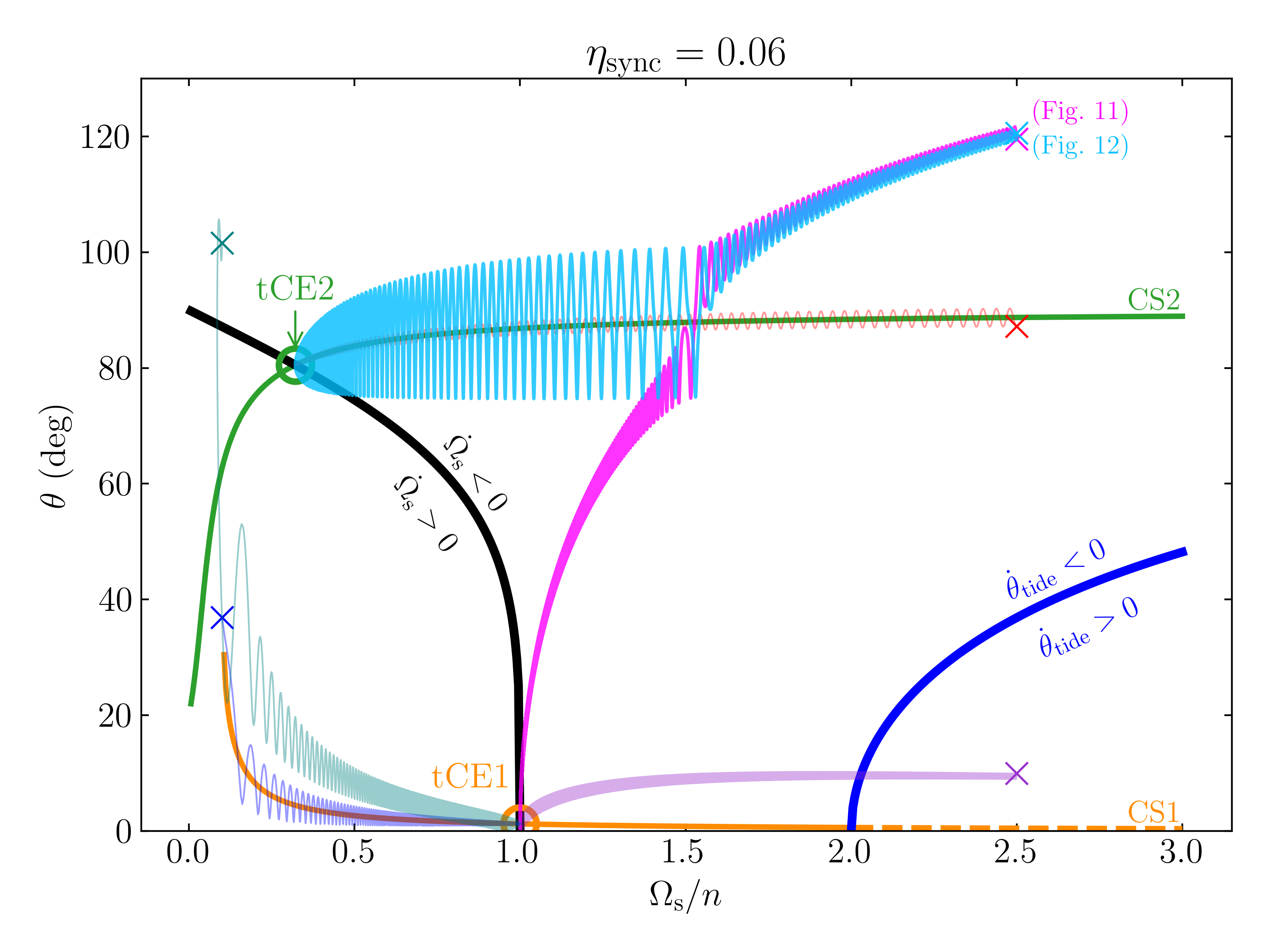
Figure 8: Schematic depiction of the effect of tidal friction on the planet’s spin evolution in the $\theta$-$\Omega_{\rm s}$ plane for a system with $I=20^{\circ}$ (corresponding to $\eta_{\rm c}=0.574$; see Eq. 7) and $\eta_{\rm sync}=0.06$ (see Eq. 39). The black and blue lines denote where the tidal $\dot{\Omega}_{\rm s}$ and $\dot{\theta}$ change signs (see Eqs. 34 and 37). The orange and green lines give the CS1 and CS2 obliquities respectively (these are the two CSs that can be stable in the presence of tidal dissipation). Note that when $\dot{\theta}_{\rm tide}>0$, CS1 becomes unstable, denoted by the dashed orange line. The points that lie on CSs and satisfy $\dot{\Omega}_{\rm s}=0$ are called tidal Cassini Equilibria (tCE), which are circled and labeled. The various colored crosses and their associated colored lines represent a few characteristic examples of the spin evolution under weak tidal friction (for illustrative purposes, we have used $\left|g\right|t_{\rm s}=10^{2}$ and evolved each example for $5t_{\rm s}$). The phase space evolution of the two thicker evolutionary trajectories (cyan and pink; those beginning at $\theta_{\rm i}=120^{\circ}$) are shown in Figs. 12–13.

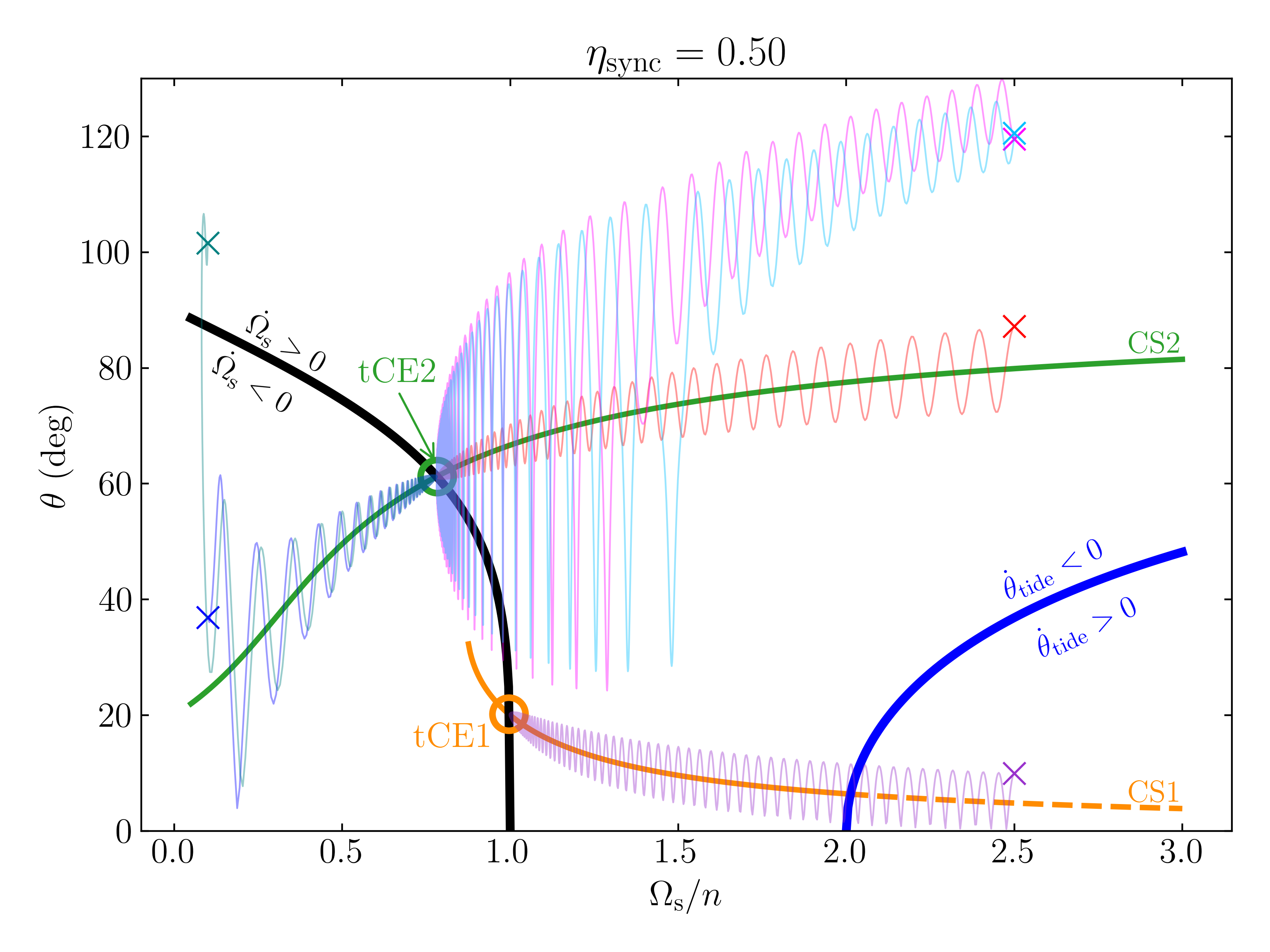
Figure 9: Same as Fig. 8 but for $\eta_{\rm sync}=0.5$. The crosses and lines correspond to evolutionary trajectories using the same initial conditions as those shown in Fig. 8.

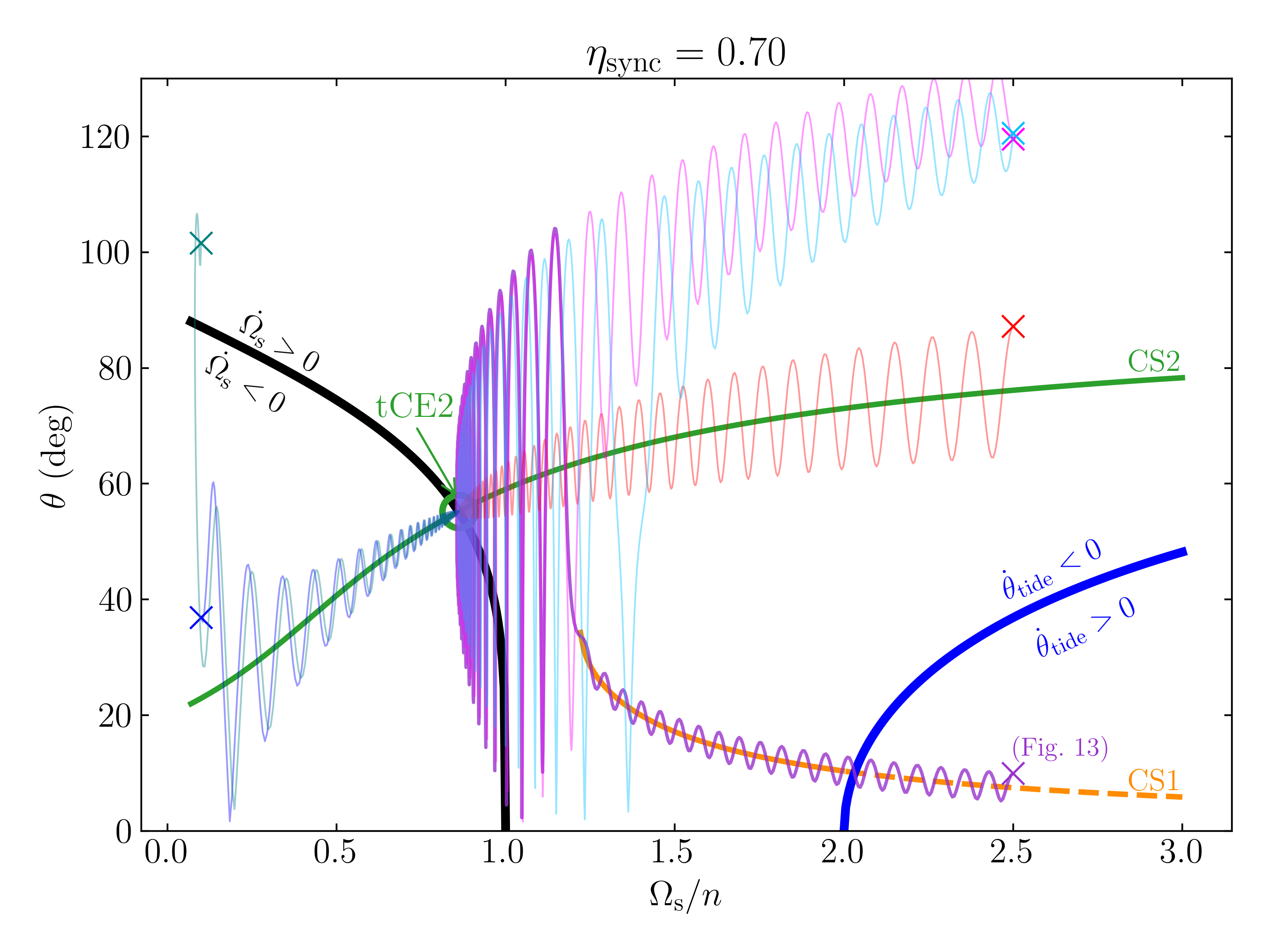
Figure 10: Same as Figs. 8 but for $\eta_{\rm sync}=0.7$. Note that $\eta_{\rm sync}=0.7>\eta_{\rm c}=0.574$ and tCE1 does not exist. The phase space evolution of the thick purple trajectory (starting at $\theta_{\rm i}=10^{\circ}$) is shown in Fig. 14.

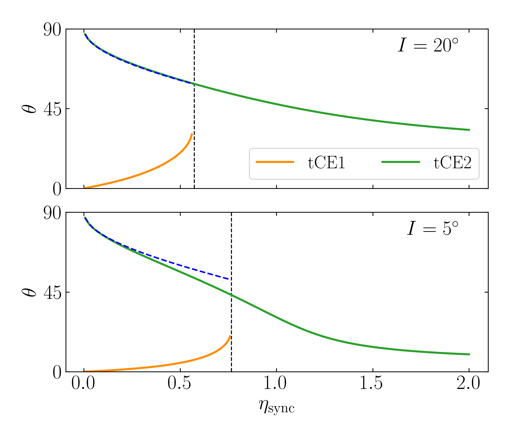
Figure 11: Obliquities of the two tCE as a function of $\eta_{\rm sync}$ (defined in Eq. 39) for $I=20^{\circ}$ (top) and $I=5^{\circ}$ (bottom). The blue dashed lines denote the analytical approximation given by Eq. (40) and is only valid for $\eta_{\rm sync}\ll 1$. The vertical dashed lines denote where $\eta_{\rm sync}=\eta_{\rm c}(I)$, above which tCE1 ceases to exist.

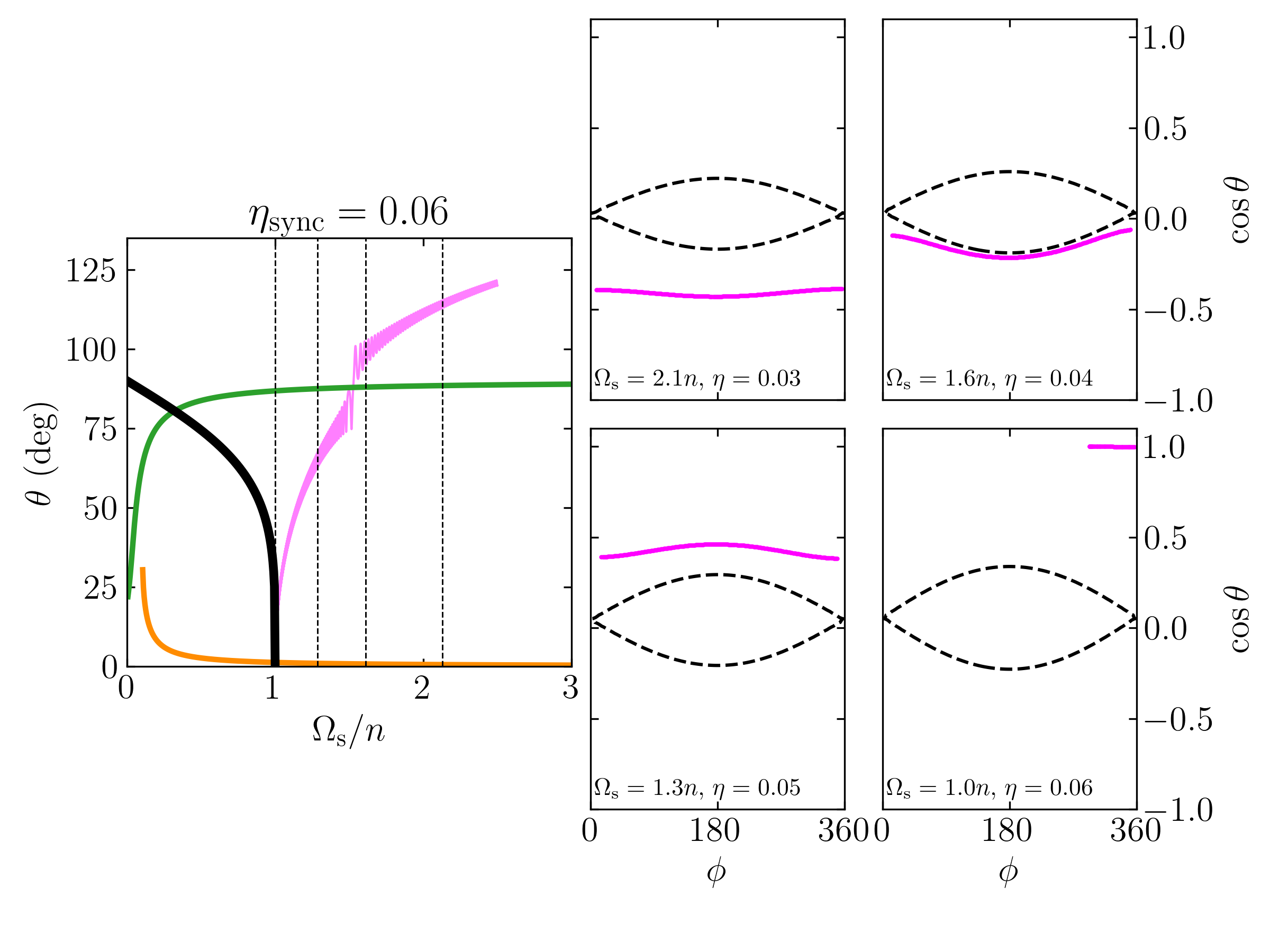
Figure 12: Phase space evolution of the pink trajectory in Fig. 8, for which $\eta_{\rm sync}=0.06$ and $I=20^{\circ}$ (corresponding to $\eta_{\rm c}=0.574$). The initial conditions are $\Omega_{\rm s,i}=2.5n$, $\theta_{\rm i}=120^{\circ}$, and $\phi_{\rm i}=0^{\circ}$, and we have used $\left|g\right|t_{\rm s}=10^{2}$ and have evolved the system for $5t_{\rm s}$. In the left-most panel, the trajectory’s evolution in the $\theta$-$\Omega_{\rm s}$ plane along with the curves indicating CS1, CS2, and $\dot{\Omega}_{\rm s}=0$ are re-displayed from Fig. 8. The vertical dashed lines denote the values of $\Omega_{\rm s}/n$ for which a few phase space snapshots of the system are displayed in the right four panels. In each of these right four panels, the trajectory’s evolution for a single circulation/libration cycle is displayed in the $\cos\theta$-$\phi$ plane for the labeled value of $\Omega_{\rm s}$ (and the corresponding value of $\eta$). The system encounters the separatrix, undergoes a III $\to$ I transition, and converges to tCE1.

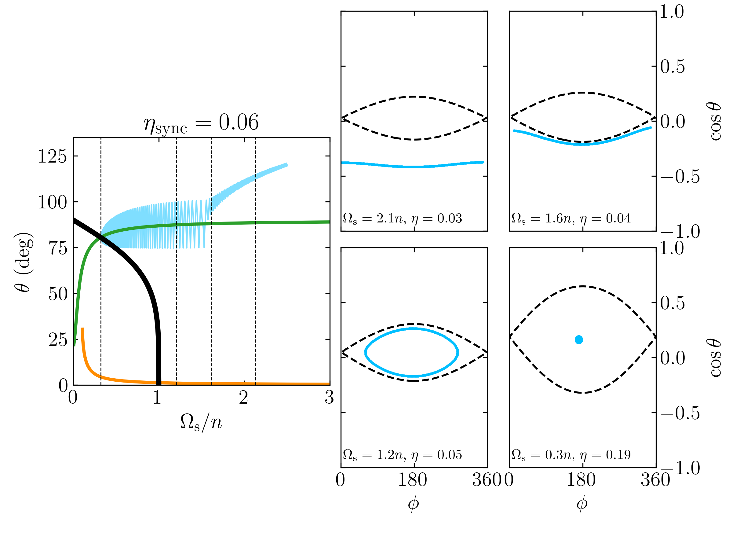
Figure 13: Same as Fig. 12 but for $\phi_{\rm i}=286^{\circ}$, corresponding to the cyan trajectory in Fig. 8. The system encounters the separatrix, undergoes a III $\to$ II transition, and converges to tCE2. The small $\phi$ offset of tCE2 from $180^{\circ}$ arises from the alignment torque (see Fig. 3). Note that the initial condition of this trajectory and that displayed in Fig. 12 have the same initial $\theta_{\rm i}$ and $\Omega_{\rm s,i}$ but different precessional phases $\phi_{\rm i}$.

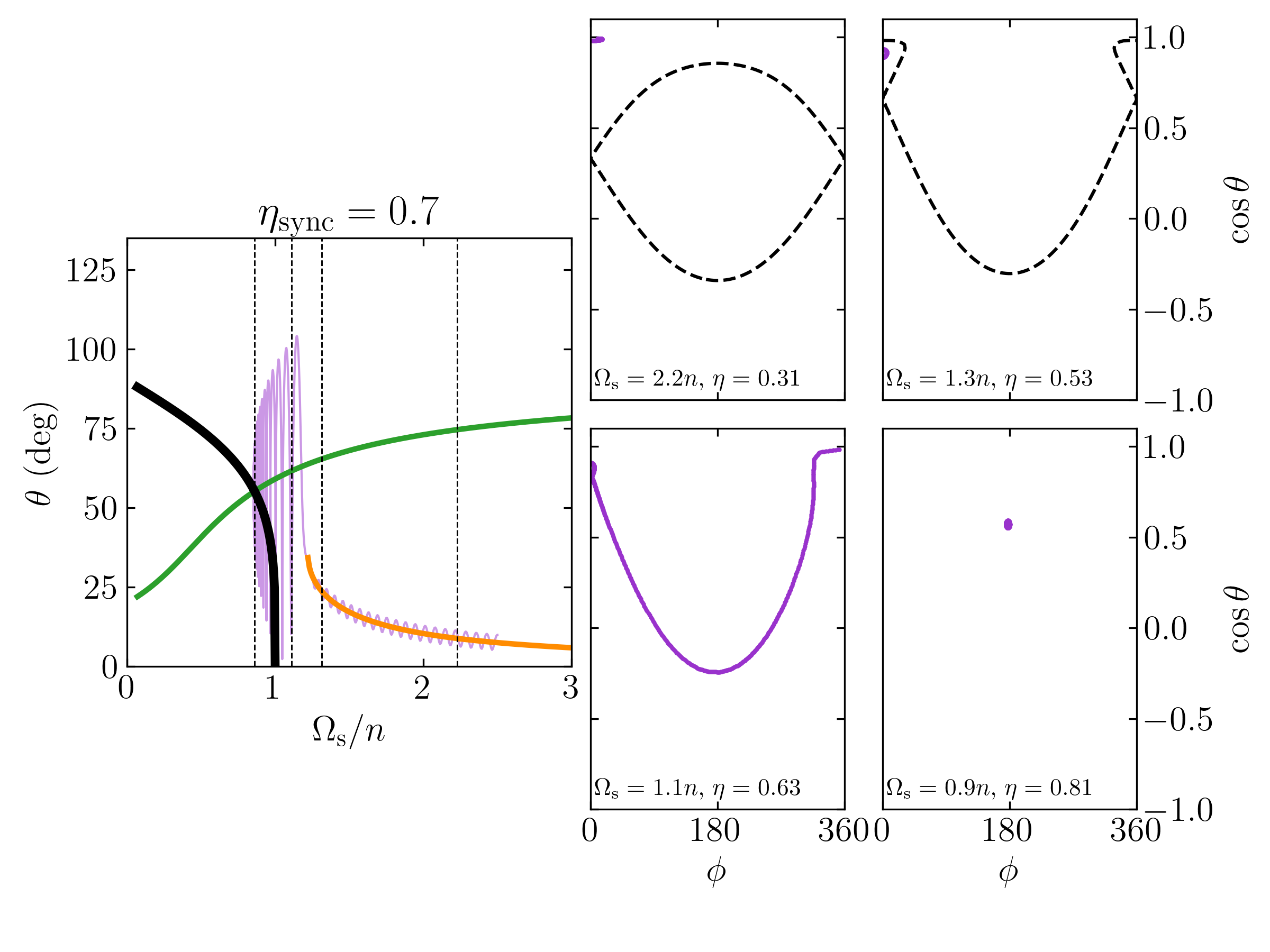
Figure 14: Same as Fig. 12 but for $\eta_{\rm sync}=0.7$ and $\theta_{\rm i}=10^{\circ}$, corresponding to the purple trajectory shown in Fig. 10. Here, the system evolves along CS1 until the separatrix disappears, upon which it experiences large obliquity variations that damp due to tidal dissipation. The highly asymmetric shape in the third panel arises due to the strong tidal dissipation used in this simulation ($\left|g\right|t_{\rm s}=10^{2}$). The system finally converges to tCE2, the only tCE that exists for this value of $\eta_{\rm sync}$.

There are two important conditions that can influence the existence and stability of the tCE. First, if $\eta_{\rm sync}>\eta_{\rm c}$ (where $\eta_{\rm c}$ is given by Eq. 7), then tCE1 will not exist (Fig. 10 gives an example). Second, tCE2 may not be stable if the phase shift due to the alignment torque (see Section 3.1) is too large. Applying the results of Section 3.2 (see Eqs. 12–13), we find that tCE2 is stable as long as $t_{\rm s}\geq t_{\rm s,c}$ where

$$t_{\rm s,c}\equiv\frac{\sin\theta_{\rm tCE2}}{\left|g\right|\sin I}\left(\frac{2n}{\Omega_{\rm s,tCE2}}-\cos\theta_{\rm tCE2}\right).$$ (42)

When $\eta_{\rm sync}\ll 1$, we can use Eqs. (40–41) to further simplify $t_{\rm s,c}$ to

$$t_{\rm s,c}\simeq\frac{\tan\theta_{\rm tCE2}}{\left|g\right|\sin I}\approx\frac{1}{\left|g\right|\sin I}\sqrt{\frac{2}{\eta_{\rm sync}\cos I}}.$$ (43)

4.2 Spin and Obliquity Evolution as a Function of Initial Spin Orientation

We can now study the final fate of the planet’s spin as a function of the initial condition. We begin by examining the example trajectories shown in Figs. 8, for which we have integrated the equations of motion (combining Eqs. 5 and 31 to give $\mathrm{d}\hat{\boldsymbol{\mathbf{s}}}/\mathrm{d}t$, and Eq. 32) and set $I=20^{\circ}$, $t_{\rm s}=100\left|g\right|^{-1}$. We discuss each of the six trajectories in turn:

• The trajectory with the initial condition $\Omega_{\rm s,i}=2.5n$ and $\theta_{\rm i}=10^{\circ}$ (purple) has an initially prograde spin (i.e. in zone I, see Fig. 2) and directly evolves to tCE1, with the final $\Omega_{\rm s}/n\simeq 1$ and $\theta=\theta_{\rm CS1}\simeq\eta_{\rm sync}\sin I$ (for $\eta_{\rm sync}\ll 1$; see Appendix A of paper I).

• The trajectory with $\Omega_{\rm s,i}=2.5n$ and $\theta_{\rm i}=90^{\circ}$ (red) has an initial condition inside the resonance / separatrix (zone II) and evolves to tCE2. Note that the obliquity is trapped in a high value due to the stability of CS2 under the alignment torque, as shown in Section 4.1.

• We have chosen two trajectories, both with the initial condition $\Omega_{\rm s,i}=2.5n$ and $\theta_{\rm i}=120^{\circ}$, but with different initial precessional phases $\phi_{\rm i}$. Consider first the pink trajectory, for which $\phi_{\rm i}=0^{\circ}$. It originates in zone III, evolves towards the separatrix as tidal friction damps the obliquity, and crosses the resonance (separatrix) without being captured, upon which the obliquity continues to damp until the system converges to tCE1. The detailed phase space evolution of this trajectory is shown in Fig. 12, where the outcome of the separatrix encounter is very visible.

• The light blue trajectory also has $\Omega_{\rm s,i}=2.5n$ and $\theta_{\rm i}=120^{\circ}$ (like the pink trajectory) but with the initial precessional phase $\phi_{\rm i}\approx 286^{\circ}$. It also originates in zone III, encounters the separatrix but is captured into the resonance (zone II), upon which tidal friction drives the system towards tCE2. The detailed phase space evolution of this trajectory is shown in Fig. 13, where the resonance capture is displayed. Also visible in the final panel of Fig. 13 is the slight phase offset of CS2, i.e. $\phi_{\rm cs}<180^{\circ}$, in agreement with the result of Section 3.1 (see Fig. 3).

• For completeness, we also examine some trajectories for initially subsynchronous spin rates. The trajectory with $\Omega_{\rm s,i}=0.1n$ and $\theta_{\rm i}=35^{\circ}$ (blue) has its obliquity rapidly damped to zero by tidal friction as it spins up to spin-orbit synchronization, eventually converging to tCE1. A subtlety of initially subsynchronous spins can be seen here: since the initial $\eta_{\rm i}=0.6>\eta_{\rm c}$ ($=0.574$), the separatrix and CS1 do not exist initially. As such, naively, one expects initial convergence to CS2 and subsequent obliquity evolution along CS2 as the spin increases. However, due to the strong tidal dissipation adapted in the calculation and the proximity of $\eta_{\rm i}$ to $\eta_{\rm c}$, CS1 appears within a single circulation cycle, and the obliquity quickly damps to, and continues to evolve along CS1.

• The trajectory with $\Omega_{\rm s,i}=0.1n$ and $\theta_{\rm i}=100^{\circ}$ (teal) also has its obliquity damped toward tCE1 as it approaches spin-orbit synchronization. We note that if we adopt $t_{\rm s}=10^{3}\left|g\right|^{-1}$, the same initial condition will converge to tCE2, agreeing with the intuitive analysis given in the previous paragraph.

In Figs. 9–10 we show, for each of the six initial conditions, the evolutionary trajectories for the $\eta_{\rm sync}=0.5$ and $\eta_{\rm sync}=0.7$ cases. The qualitative behaviors of these six examples change in several important ways, so we will discuss a few points of interest:

• For both $\eta_{\rm sync}=0.5$ and $\eta_{\rm sync}=0.7$, we see that the initial conditions with $\theta_{\rm i}=120^{\circ}$ ($\phi_{\rm i}=0$, pink; and $\phi_{\rm i}=286^{\circ}$, blue) converge to tCE2. In fact, for these values of $\eta_{\rm sync}$, all initial conditions with $\theta_{\rm i}=120^{\circ}$ will converge to tCE2 regardless of $\phi_{\rm i}$.

• The two subsynchronous initial conditions evolve to tCE2 for both $\eta_{\rm sync}=0.5$ and $\eta_{\rm sync}=0.7$, as in both cases $\eta_{\rm i}\gg\eta_{\rm c}$ and CS2 is the only low-obliquity spin equilibrium. The system then continues to evolve along CS2 toward tCE2.

• Of particular interest is the trajectory starting from the initial condition $\Omega_{\rm s,i}=2.5n$ and $\theta_{\rm i}=10^{\circ}$ (purple) in the case of $\eta_{\rm sync}=0.7$. Figure 14 shows the detailed phase space evolution of this trajectory, where it can be seen that the system initially evolves along the stable CS1, but is ejected when $\Omega_{\rm s}$ becomes sufficiently small that CS1 ceases to exist, upon which large obliquity variations eventually lead to convergence to tCE2, the only tCE that exists.

From the above examples, we see that the spin evolution driven by tides can be complex and varies greatly depending on the various system parameters and initial conditions. In the case where the initial spin is subsynchronous, the detailed outcome depends sensitively on the initial value of $\eta$ and the tidal dissipation rate. In the following, we restrict our discussion to the more astrophysically common regime of $\Omega_{\rm s,i}\gg n$, and we adopt the fiducial value $\Omega_{\rm s,i}=10n$.

Having developed an intuition for a few different possible evolutionary trajectories, we can attempt to draw general conclusions about the final fate of the planet’s spin as a function of its initial conditions. We do this by again integrating Eqs. (5, 31–32) for many initial $\theta_{\rm i}$ and $\phi_{\rm i}$ and examining the final outcomes. In contrast to the examples shown in Figs. 8–14, we use a more gradual tidal dissipation rate of $\left|gt_{\rm s}\right|=10^{3}$. In Fig. 15, we show the final outcome for many randomly chosen $\theta_{\rm i}$ and $\phi_{\rm i}$ for $\eta_{\rm sync}=0.06$ and $I=20^{\circ}$. We see that the behaviors seen in the example trajectories of Fig. 8 are general: tCE1 is generally reached for spins initially in zone I (like the purple trajectory in Fig. 8), tCE2 is generally reached for spins initially in zone II (like the red trajectory in Fig. 8), and a probabilistic outcome is observed for spins initially in zone III (like the light blue and pink trajectories in Fig. 8). Figures 16 and 17 show similar results for $\eta_{\rm sync}=0.2$ and $\eta_{\rm sync}=0.5$. As $\eta_{\rm sync}$ is increased, more initial conditions reach tCE2. This is both because there are more systems initially in zone II and because systems initially in zone III have a higher probability of executing a III $\to$ II transition upon separatrix encounter. Note also that in Fig. 17, even initial conditions in zone I are able to reach tCE2; we comment on the origin of this behavior in the next section.

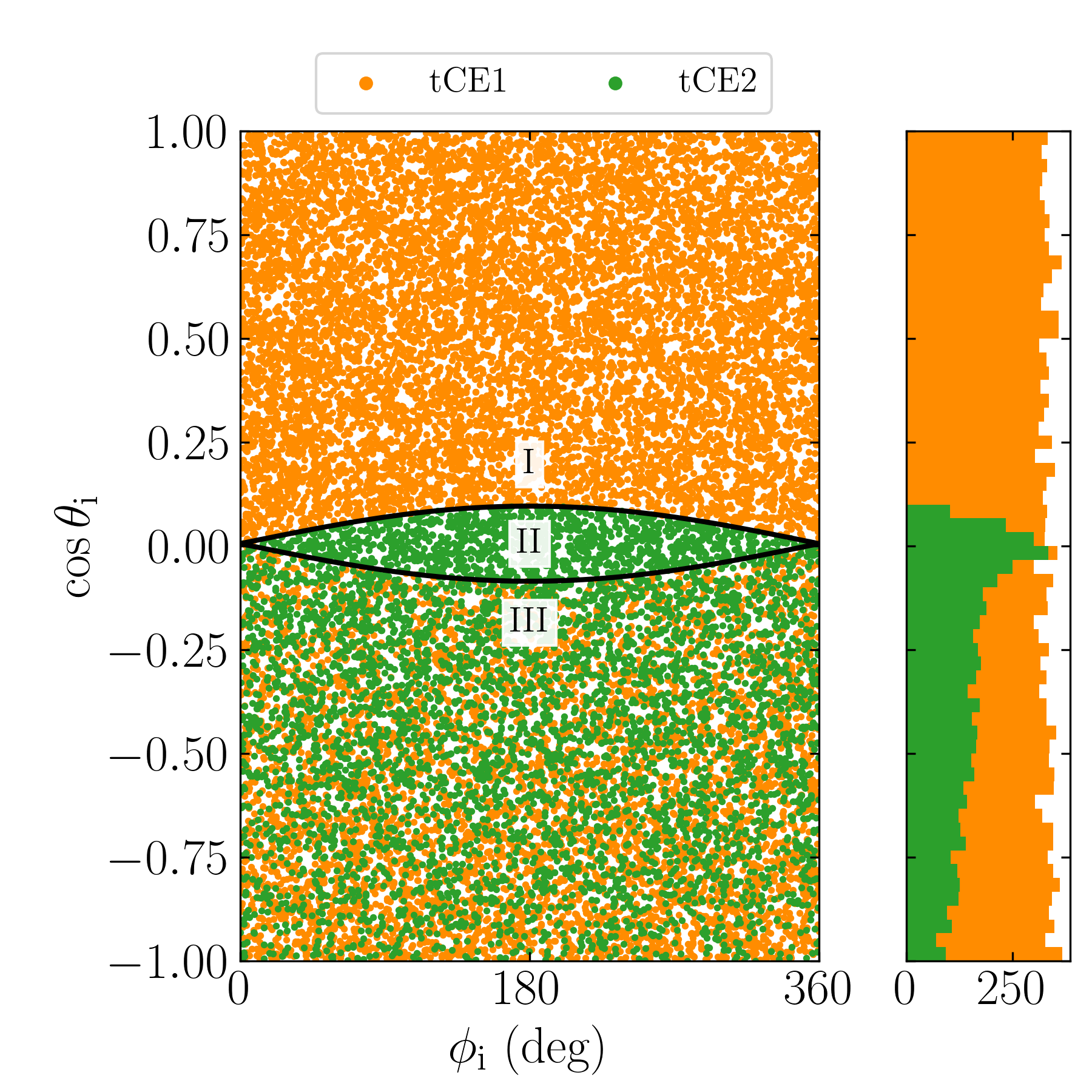
Figure 15: Left: Asymptotic outcomes of spin evolution in the presence of weak tidal friction for different initial spin orientations ($\theta_{\rm i}$ and $\phi_{\rm i}$) for a system with $\eta_{\rm sync}=0.06$ and $I=20^{\circ}$. Each dot represents an initial spin orientation, and the coloring of the dot indicates which tCE (legend) the system evolves into. Similarly to Fig. 5 initial conditions in Zone I evolve into CS1, those in Zone II evolve into CS2, and those in Zone III have a probabilistic outcome. Right: Histogram of the final tCE that a given initial obliquity $\theta_{\rm i}$ evolves into, averaged over $\phi_{\rm i}$.

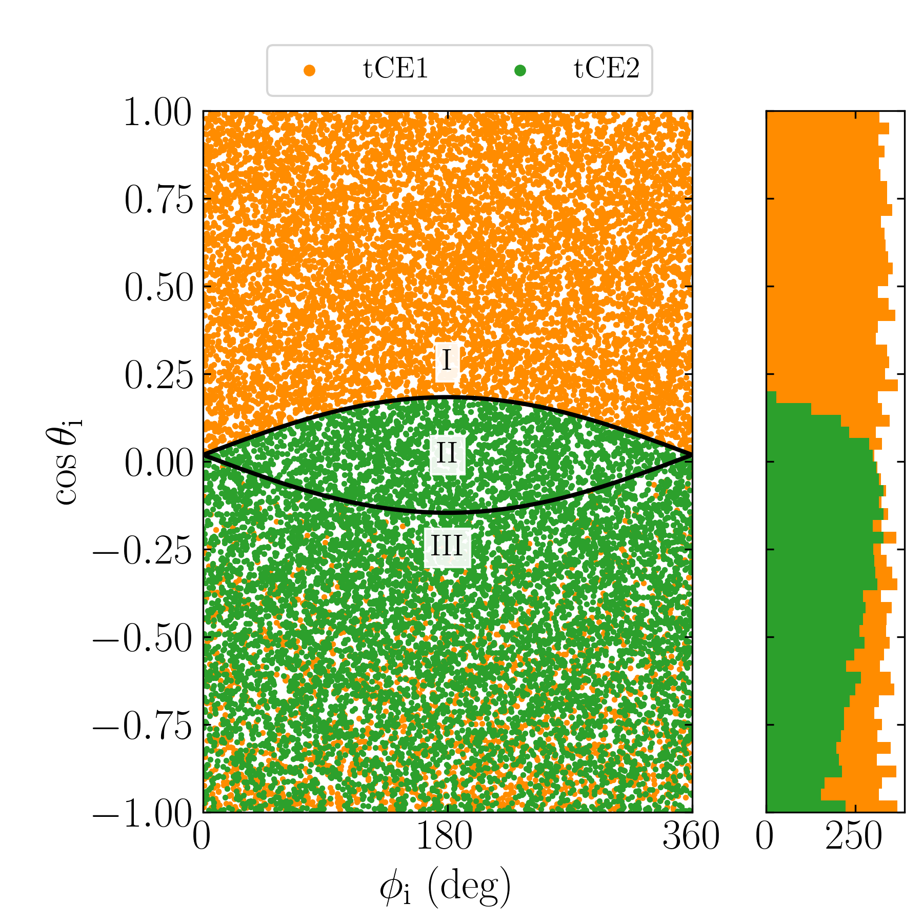
Figure 16: Same as Fig. 15 but for $\eta_{\rm sync}=0.2$.

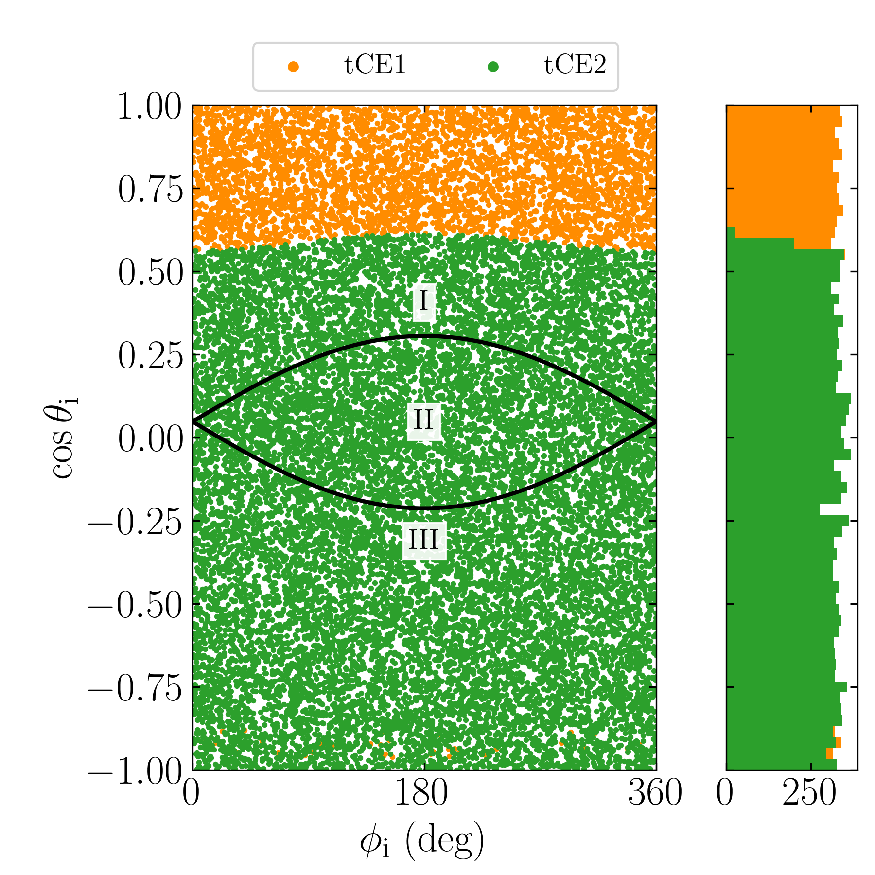
Figure 17: Same as Fig. 15 but for $\eta_{\rm sync}=0.5$. Note that even points above the separatrix can evolve towards tCE2 here.

4.3 Semi-analytical Calculation of Resonance Capture Probability

Even when including the evolution of $\Omega_{\rm s}$, and therefore the parameter $\eta$ (see Eq. 6), the probabilities of the III $\to$ I and III $\to$ II transitions upon separatrix encounter can still be obtained semi-analytically. The calculation resembles that presented in Section 3.4 but involves several new ingredients. We describe the calculation below.

In Section 3.4, we found that the evolution of $H$, the value of the unperturbed Hamiltonian, allowed us to calculate the probabilities of the various outcomes of separatrix encounter. Specifically, the outcome upon separatrix encounter is determined by the value of $H$ at the start of the separatrix-crossing orbit relative to $H_{\rm sep}$, the value of $H$ along the separatrix. However, when the spin $\Omega_{\rm s}$ is also evolving, $H_{\rm sep}$ also changes during the separatrix-crossing orbit, and the calculation in Section 3.4 must be generalized to account for this. Instead of focusing on the evolution of $H$ along a trajectory, we instead follow the evolution of

$$K\equiv H-H_{\rm sep}.$$ (44)

Note that $K>0$ inside the separatrix, and $K<0$ outside. With this modification, the outcome of the separatrix-crossing orbit can be determined in the same way as in Section 3.4. First, we must compute the change in $K$ along the legs of the separatrix. We define $\Delta K_{\pm}$ by generalizing Eq. (20) in the natural way:

$$\Delta K_{\pm} =\oint_{\mathcal{C}_{\pm}}\left[\frac{\mathrm{d}H}{\mathrm{d}t}-\frac{\mathrm{d}H_{\rm sep}}{\mathrm{d}t}\right]\;\mathrm{d}t.$$ (45)

Here, however, note that the contours $\mathcal{C}_{\pm}$ depends on the value of $\Omega_{\rm s}$ at separatrix encounter (or the corresponding value $\eta=\eta_{\rm cross}$). Since there is no closed form solution for $\Omega_{\rm s}(t)$, the probabilities of the various outcomes cannot be expressed as a simple function of the initial conditions.

Continuing the argument presented in Section 3.4, we consider the outcome of the separatrix-crossing orbit as a function of $K_{i}$, the value of $K$ at the start ($\phi=0$) of the separatrix-crossing orbit. We find that if $-\Delta K_{+}-\Delta K_{-}<I_{\rm i}<0$, then the system undergoes a III $\to$ II transition and eventually evolves towards tCE2, and if $-\Delta K_{-}<K_{i}<-\Delta K_{-}-\Delta K_{+}$, then the system undergoes a III $\to$ I transition and ultimately evolves towards tCE1. Thus, we find that the probability of a III $\to$ II transition is given by

$$P_{\rm III\to II}=\frac{\Delta K_{+}+\Delta K_{-}}{\Delta K_{-}}.$$ (46)

Again, since $\Delta K_{\pm}$ are evaluated at resonance encounter, and $\Omega_{\rm s}$ is evolving, there is no way to express $\Delta K_{\pm}$ in a closed form of the initial conditions. In fact, since many resonance encounters occur when $\eta=\eta_{\rm cross}$ is $\gtrsim 0.2$, even an approximate calculation of $\Delta K_{\pm}$ using Eq. (27) (which is valid only for $\eta\ll 1$) is inaccurate, and we instead calculate $\Delta K_{\pm}$ along the numerically-computed $\mathcal{C}_{\pm}$ for arbitrary $\eta$. Note that Eqs. (45, 46) are equivalent to the separatrix capture result of Henrard (1982) when $\dot{\theta}_{\rm tide}=0$ (see also Henrard & Murigande, 1987 and Paper I). In other words, we argue that this classic calculation can be unified with the calculation given in Section 3.4 to give an accurate prediction of separatrix encounter outcome probabilities in the presence of both dissipative perturbation and parametric evolution of the Hamiltonian.

We note that Levrard et al. (2007) also presented an analytical expression for the resonance capture probability (their Eq. 14) following the method of Goldreich & Peale (1966). However, their expression is incomplete, as it does not account for the contribution of the tidal alignment torque to the change of the integral of motion over a single orbit.

To validate the accuracy of Eq. (46), we can compare with direct numerical integration of Eqs. (5, 31–32) for many initial conditions while evaluating $P_{\rm III\to II}$ (and thus also obtaining $P_{\rm III\to I}=1-P_{\rm III\to II}$) for each simulation at the moment it encounters the separatrix, if it does so. If the theory is correct, the total numbers of systems converging to each of tCE1 and tCE2 should be equal to those predicted by the calculated probabilities. In Fig. 18, we show the agreement of this semi-analytic procedure with the numerical result displayed in the right panel of Fig. 15. Figure 19 depicts the same for the parameters of Figs. 16, also showing satisfactory agreement. Thus, we conclude that the outcomes of separatrix encounter are accurately predicted by Eq. (46).

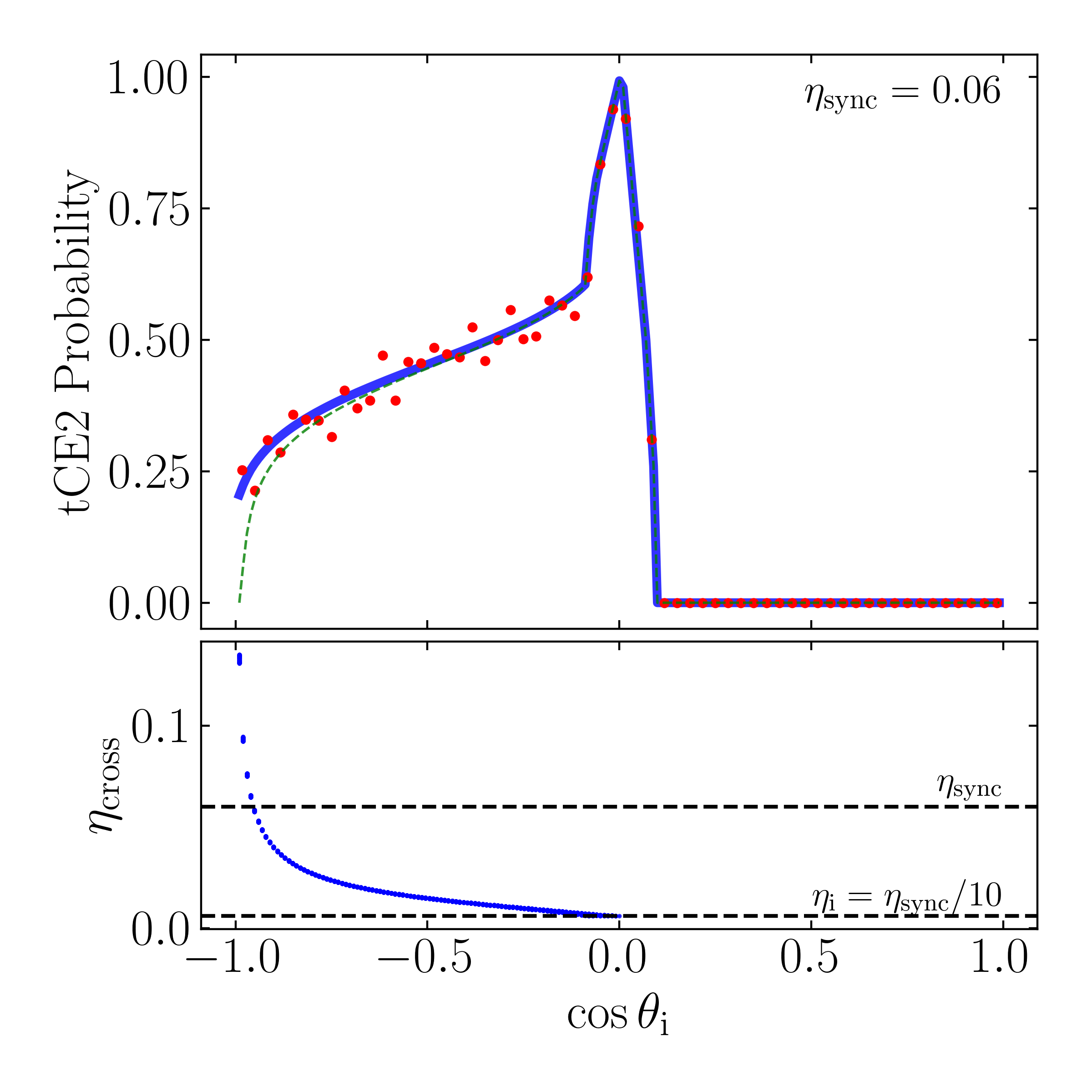
Figure 18: Comparison of the fraction of systems converging to tCE2 obtained via numerical simulation (red dots) and obtained via a semi-analytic calculation (blue line) for $\eta_{\rm sync}=0.06$, $I=20^{\circ}$, and $\Omega_{\rm s,i}=10n$ (see right panel of Fig. 15). The semi-analytic calculation is performed by numerically integrating Eqs. (5, 31–32) on a grid of initial conditions uniform in $\cos\theta_{\rm i}$ and $\phi_{\rm i}$ until the system reaches the separatrix, then calculating the probability of reaching tCE2 for each integration using Eq. (46). The green dashed line in the top panel shows the result of using the analytical expression (Eq. 74) for $\Delta K_{\pm}$, and the bottom panel shows the distribution of values of $\eta_{\rm cross}$, the value of $\eta$ when a trajectory starting at $\theta_{\rm i}$ encounters the separatrix.

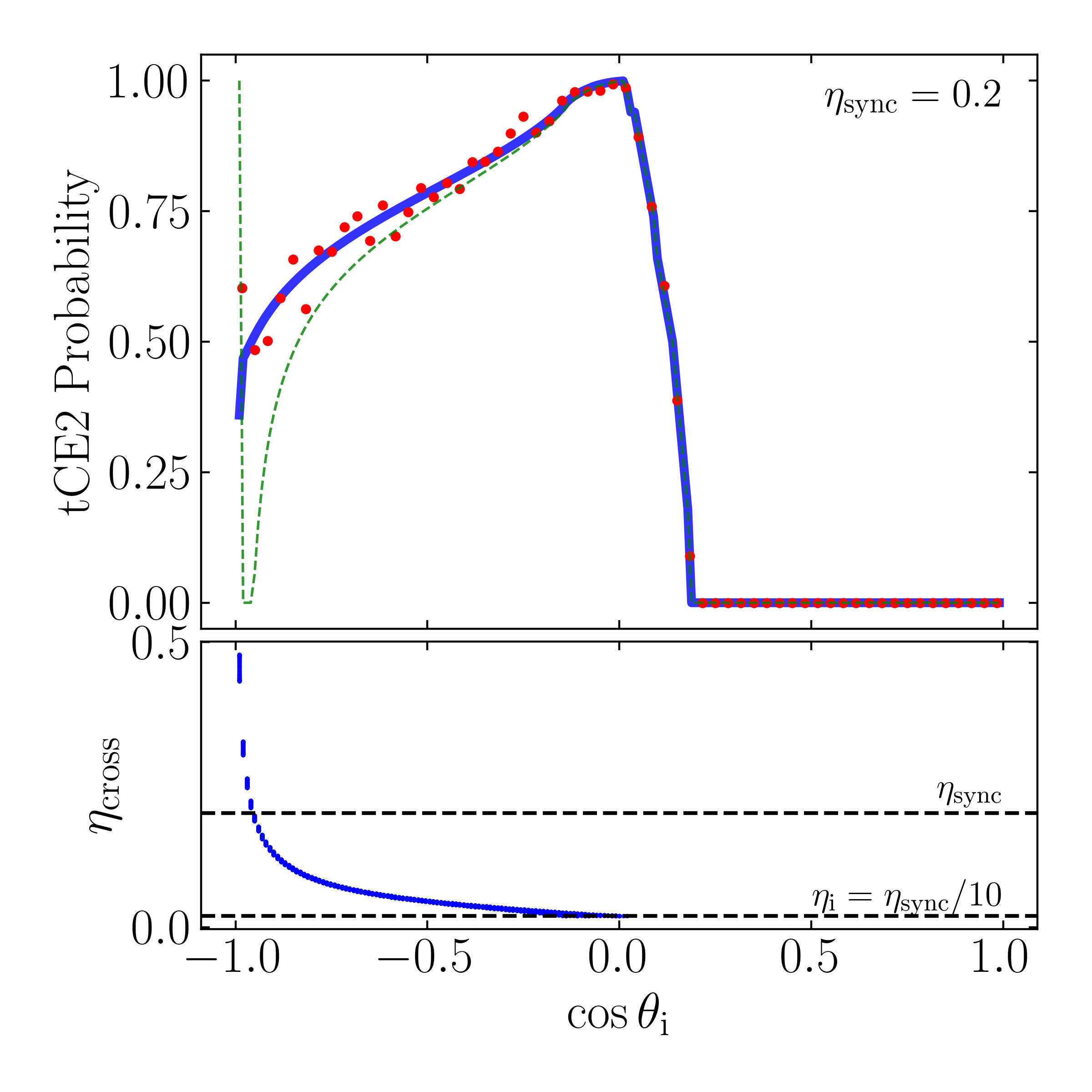
Figure 19: Same as Fig. 18 but for $\eta_{\rm sync}=0.2$, corresponding to the right panel of Fig. 16. Note that the analytical equation (Eq. 74; green dashed line) exhibits significantly poorer agreement than in Fig. 18 when $\eta_{\rm cross}\gtrsim 0.2$.

With the above calculation, we can understand why even some initial conditions in zone I may converge to tCE2 in certain situations (see Fig. 17). As long as the initial spin is sufficiently large ($\geq 2n$), Eq. (34) shows that when $\cos\theta>2n/\Omega_{\rm s}$, the obliquity can increase. In particular, when the critical obliquity $\cos\theta=2n/\Omega_{\rm s}$ is inside the separatrix, tidal alignment acts to drive initial conditions in both zones I and III towards the critical obliquity and into the separatrix, and also towards larger $H$. As such, when this effect is sufficiently strong, Eq. (45) shows that both $\Delta K_{\pm}>0$, and both III $\to$ II and I $\to$ II transitions are guaranteed upon separatrix encounter (Eq. 46).

4.4 Spin Obliquity Evolution for Isotropic Initial Spin Orientations

In Sections 4.2–4.3, we considered the outcome of the spin evolution driven by tidal torque as a function of the initial spin orientation, specified by $\theta_{\rm i}$ and $\phi_{\rm i}$. Here, we calculate the probability of evolution into tCE2 when averaging over a distribution of initial spin orientations, which we denote by $P_{\rm tCE2}$. For simplicity, we assume $\hat{\boldsymbol{\mathbf{s}}}$ to be isotropically distributed (see Section 6 for discussions concerning impact of more physically realistic distributions of $\hat{\boldsymbol{\mathbf{s}}}$). The bottom panel of Fig. 20 shows $P_{\rm tCE2}$ for $I=20^{\circ}$ as a function of $\eta_{\rm sync}$. We see that, e.g., tCE2 with a large obliquity ($\sim 70^{\circ}$) can be reached with substantial probability ($\gtrsim 50\%$).

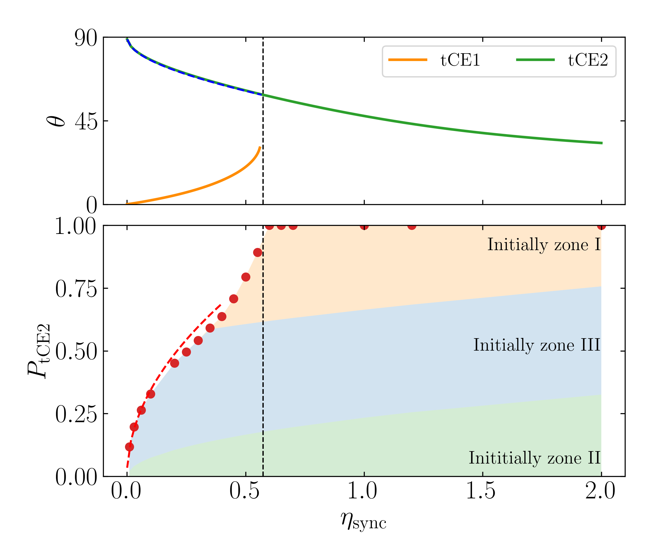
Figure 20: Top: Same as top panel of Fig. 11. Bottom: Total probability of the system ending up in tCE2 ($P_{\rm tCE2}$; red dots) as a function of $\eta_{\rm sync}$ (Eq. 39), averaged over an isotropic initial spin orientation and taking $\Omega_{\rm s,i}=10n$. The red dashed line shows the analytical prediction Eq. (47). The three shaded regions denote the contributions of initial conditions in zones I/II/III (labeled) to the total tCE2 probability. For example, among systems that converge to tCE2 for $\eta_{\rm sync}=0.06$, more originate in zone III than zone II, and none originate in zone I.

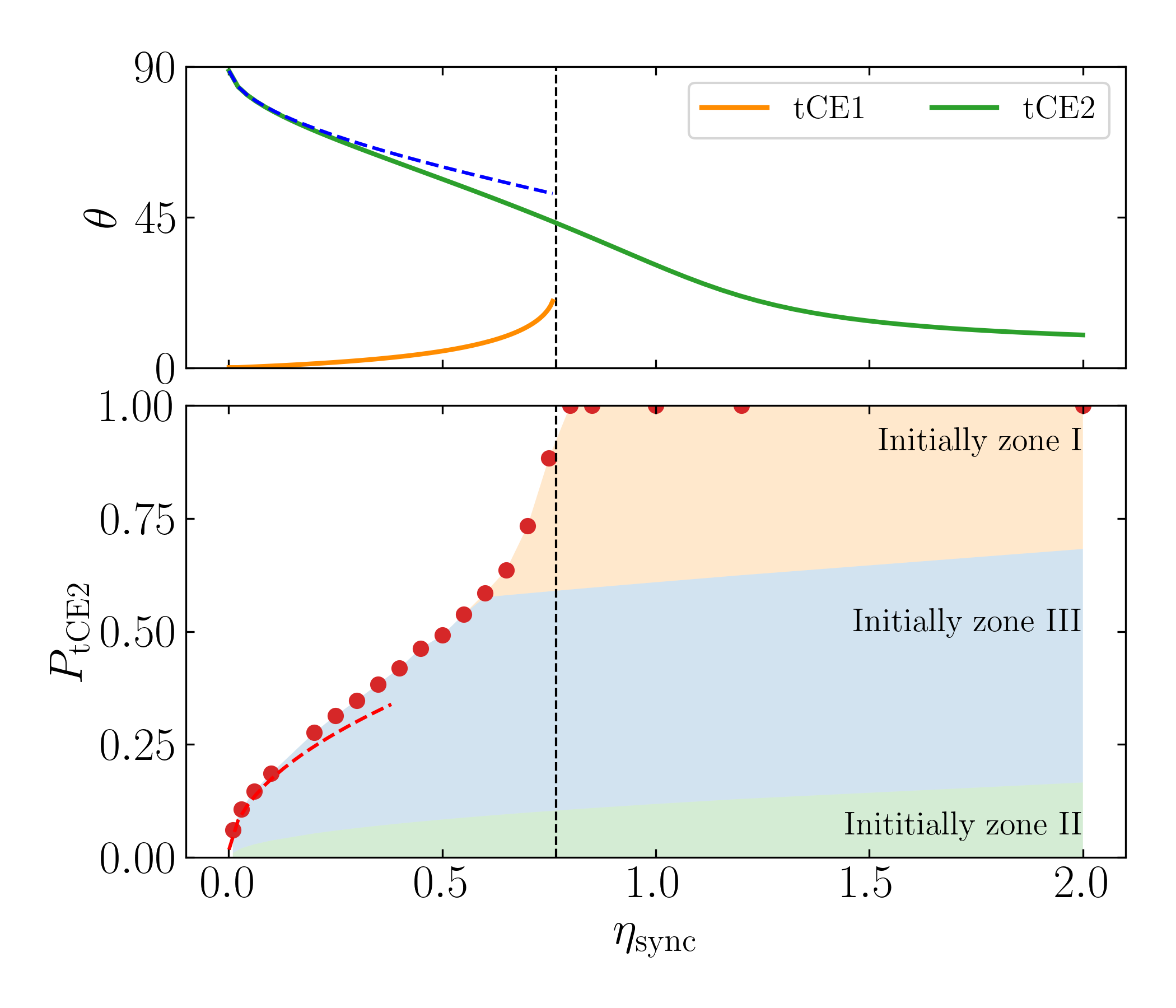
Figure 21: Same as Fig. 20 but for $I=5^{\circ}$.

When $\eta_{\rm sync}\ll 1$ and $\Omega_{\rm s,i}\gtrsim n$, an approximate analytical formula for $P_{\rm tCE2}$ can be obtained (see Appendix B):

$$P_{\rm tCE2} \simeq\frac{4\sqrt{\eta_{\rm sync}\sin I}}{\pi}\left[\sqrt{n/\Omega_{\rm s,i}}+\frac{3}{2\left(1+\sqrt{n/\Omega_{\rm s,i}}\right)}\right].$$ (47)

Eq. (47) is shown in Figs. 20–21 as the red dashed lines; it agrees well with the numerical results (red dots) for $\eta_{\rm sync}\lesssim 0.4$. To illustrate the predicted values of $P_{\rm tCE2}$ for small $\eta_{\rm sync}$, we display $P_{\rm tCE2}$ for $\eta_{\rm sync}\in\left[10^{-4},0.4\right]$ for both $I=20^{\circ}$ and $I=5^{\circ}$ in Fig. 22. Note that for $\eta_{\rm sync}\leq 10^{-2}$, numerical results for $P_{\rm tCE2}$ are difficult to obtain, as the integration of Eqs. (34)–(36) slows down dramatically due to the rapid precession of $\hat{\boldsymbol{\mathbf{s}}}$ about $\hat{\boldsymbol{\mathbf{l}}}$.

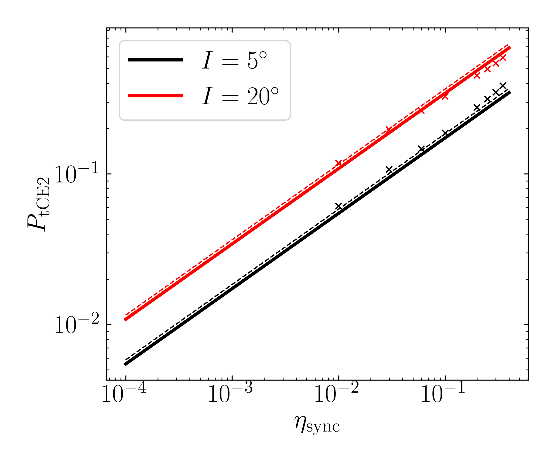
Figure 22: $P_{\rm tCE2}$ as a function of $\eta_{\rm sync}$ for $I=5^{\circ}$ and $I=20^{\circ}$ shown on a log-log plot, to emphasize the scaling at small $\eta_{\rm sync}$. The crosses are the results of numerical integrations as shown in Figs. 20–21, the solid lines are Eq. (47) for $\Omega_{\rm s,i}=10n$ and the dashed lines are for $\Omega_{\rm s,i}=3n$.

5 Applications

5.1 Obliquities of Super-Earths with Exterior Companions

Consider a system consisting of an inner Super-Earth (SE) with semi-major axis $a\lesssim 0.5\;\mathrm{AU}$ and an exterior companion. For concreteness, we assume the companion (with mass $m_{\rm p}$) to be a cold Jupiter (CJ) with $a_{\rm p}\gtrsim 1\;\mathrm{AU}$. Such systems are quite abundant (Zhu & Wu, 2018; Bryan et al., 2019). A phase of giant impacts may occur in the formation of such SEs (Inamdar & Schlichting, 2015; Izidoro et al., 2017), leading to a wide range of initial obliquities for the SEs. We are interested in the “final” obliquities of the SEs driven by tidal dissipation.

For typical SE parameters, the spin evolution timescale due to tidal dissipation is given by

$$\frac{1}{t_{\rm s}}\simeq{} \frac{1}{3\times 10^{7}\;\mathrm{yr}}\left(\frac{1}{4k}\right)\left(\frac{2k_{2}/Q}{10^{-3}}\right)\left(\frac{M_{\star}}{M_{\odot}}\right)^{3/2}\left(\frac{m}{4M_{\oplus}}\right)^{-1}$$

$$\times\left(\frac{R}{2R_{\oplus}}\right)^{3}\left(\frac{a}{0.4\;\mathrm{AU}}\right)^{-9/2}.$$ (48)

This occurs well within the age of SE-CJ systems. On the other hand, the orbital evolution of the SE occurs on the timescale (e.g. Lai, 2012)

$$-\frac{\dot{a}}{a}={} \frac{3k_{2}}{Q}\frac{M_{\star}}{m}\left(\frac{R}{a}\right)^{5}n\left(1-\frac{\Omega_{\rm s}}{n}\cos\theta\right)$$

$$\simeq{} \frac{1}{7\times 10^{14}\;\mathrm{yr}}\left(1-\frac{\Omega_{\rm s}}{n}\cos\theta\right)\left(\frac{2k_{2}/Q}{10^{-3}}\right)\left(\frac{M_{\star}}{M_{\odot}}\right)^{3/2}$$

$$\times\left(\frac{m}{4M_{\oplus}}\right)^{-1}\left(\frac{R}{2R_{\oplus}}\right)^{5}\left(\frac{a}{0.4\;\mathrm{AU}}\right)^{-13/2}.$$ (49)

Thus, $a$ does not evolve within the age of the SE-CJ system (for $a\gtrsim 0.06\;\mathrm{AU}$), and we shall treat $a$ as a constant in this subsection (but see Sections 5.2–5.3). With typical SE-CJ parameters, Eq. (39) can be evaluated:

$$\eta_{\rm sync}={} 0.303\cos I\left(\frac{k}{k_{\rm q}}\right)\left(\frac{m_{\rm p}}{M_{\rm J}}\right)\left(\frac{m}{4M_{\oplus}}\right)\left(\frac{M_{\star}}{M_{\odot}}\right)^{-2}\left(\frac{a}{0.4\;\mathrm{AU}}\right)^{6}$$

$$\times\left(\frac{a_{\rm p}}{5\;\mathrm{AU}}\right)^{-3}\left(\frac{R}{2R_{\oplus}}\right)^{-3}.$$ (50)

We see from Figs. 20 and 21 that this value of $\eta_{\rm sync}$ can lead to a high-obliquity tCE2 with significant probability, assuming the SE has a wide range of initial obliquities. In addition, Eq. (43) shows that tCE2 is stable if $t_{\rm s}\gtrsim t_{\rm s,c}$, where

$$\frac{1}{t_{\rm s,c}}={} \frac{\sin I\cos^{2}I}{3\times 10^{5}\;\mathrm{yr}}\left(\frac{k}{k_{\rm q}}\right)\left(\frac{m_{\rm p}}{M_{\rm J}}\right)^{3/2}\left(\frac{m}{4M_{\oplus}}\right)^{1/2}$$

$$\times\left(\frac{M_{\star}}{M_{\odot}}\right)^{-3/2}\left(\frac{a}{0.4\;\mathrm{AU}}\right)^{6}\left(\frac{a_{\rm p}}{5\;\mathrm{AU}}\right)^{-9/2}\left(\frac{R}{2R_{\oplus}}\right)^{-3/2}.$$ (51)

In Fig. 23, we show the value of $\eta_{\rm sync}$ in the regions of $\left(a,a_{\rm p}\right)$ parameter space that satisfy the stability condition for tCE2. We see that a generous portion of parameter space is able to generate and sustain SEs in stable tCE2 with significant obliquities. In summary, we predict that a large fraction of SEs with exterior CJ companions can have long-lived, significant obliquities ($\gtrsim 60^{\circ}$) due to being trapped in tCE2.

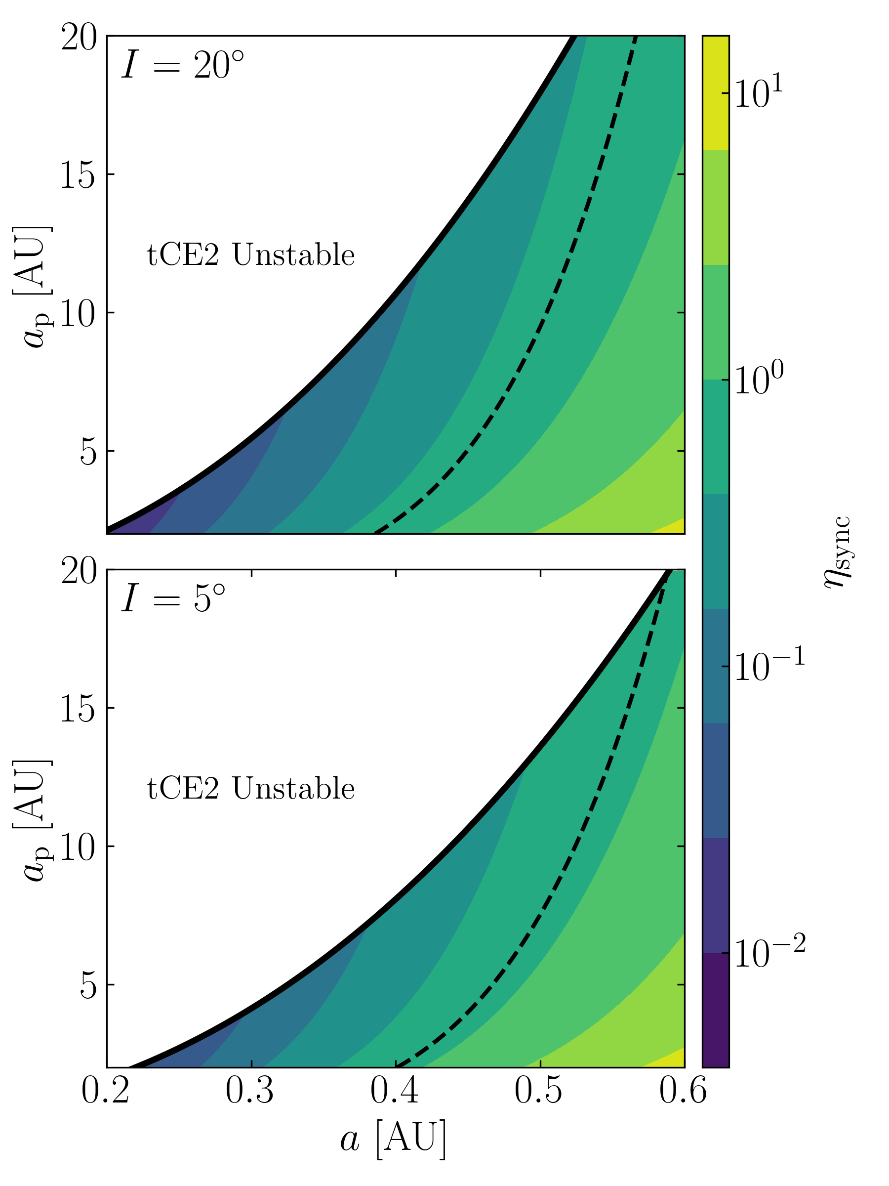
Figure 23: Depiction of the values of $\eta_{\rm sync}$ for the Super Earth + Cold Jupiter systems as a function of $a$ and $a_{\rm p}$ for $I=20^{\circ}$ (top) and $I=5^{\circ}$ (bottom). The SE is taken to have $m=4M_{\oplus}$ and $R=2R_{\oplus}$ while the CJ is taken to have $m_{\rm p}=M_{\rm J}$, and we have taken $k\approx k_{\rm q}$ for the SE. We only show the regions satisfying $t_{\rm s}\geq t_{\rm s,c}$ (the stability condition for tCE2; Eqs. 48–51). The line satisfying $\eta_{\rm sync}=\eta_{\rm c}$ (Eq. 7) is shown as the black dashed line. Systems with $\eta_{\rm sync}\gtrsim 0.1$ have appreciable probabilities of being captured in permanent tCE2 with significant obliquities (see Figs. 20–22).

5.2 Formation of Ultra-short-period Planet Formation via Obliquity Tides

Ultra-short period planets (USPs), Earth-sized planets with sub-day periods, constitute a statistically distinct subsample of Kepler planets (e.g. Winn et al., 2018; Dai et al., 2018). It is generally thought that USPs evolved from close-in SEs through orbital decay, driven by tidal dissipation in their host stars (Lee & Chiang, 2017) or in the planets (Petrovich et al., 2019; Pu & Lai, 2019). In particular, Pu & Lai (2019) showed that a “low-eccentricity migration” mechanism can successfully produce USPs with the observed properties. In this scenario, USPs evolve from a subset of SE systems: a low-mass planet with an initial period of a few days maintains a small but finite eccentricity due to secular forcings from exterior companion planets (SEs or sub-Neptunes) and evolve to become a USP due to orbital decay driven by tidal dissipation.

Millholland & Spalding (2020) proposed an alternative formation mechanism of USPs based on obliquity tides (instead of eccentricity tides as in Pu & Lai, 2019). This mechanism consists of three stages:

• A proto-USP (with two external companions) is assumed to be rapidly captured into CS2 with appreciable obliquity and a pseudo-synchronous spin rate.

• The inner planet undergoes runaway tidal migration as a result of the decreasing semi-major axis and increasing obliquity while following CS2.

• The inward migration stalls when the tidal torque becomes sufficiently strong to destroy CS2.

Here, we evaluate the viability of the obliquity-driven migration scenario for USPs using the general results presented earlier in this paper.

First, the spin evolution timescale for typical proto-USP parameters is

$$\frac{1}{t_{\rm s}}={} \frac{1}{1200\;\mathrm{yr}}\left(\frac{1}{4k}\right)\left(\frac{2k_{2}/Q}{10^{-3}}\right)\left(\frac{M_{\star}}{M_{\odot}}\right)^{3/2}\left(\frac{\rho}{\rho_{\oplus}}\right)^{-1}\left(\frac{a}{0.035\;\mathrm{AU}}\right)^{-9/2}.$$ (52)

where $\rho$ is the density of the proto-USP, $\rho_{\oplus}$ is the density of the Earth, and we have adopted the (approximately) largest possible value for $a$ (the semi-major axis of the proto-SE) to ensure that orbital decay can happen within the age of the system (see Eq. 56). This is much shorter than the age of the system, and so the proto-USP can quickly evolve into one of the stable tCE (either tCE1 or tCE2).

Next, to determine which tCE the planet evolves into, we need to evaluate $\eta_{\rm sync}$ (see Eq. 39). For simplicity, we consider the case where the proto-USP is surrounded by a single external planetary companion with $a_{\rm p}\gtrsim a$ (typical of Kepler multi-planet systems) but with $L_{\rm p}\gg L$ (this condition can easily be relaxed; see Section 5.3). To account for such a close-by companion, Eq. (4) must be modified to (see e.g. Lai & Pu, 2017):

$$\omega_{\rm lp}=\frac{3m_{\rm p}}{4M_{\star}}\left(\frac{a}{a_{\rm p}}\right)^{3}nf(\alpha),$$ (53)

where $\alpha=a/a_{\rm p}$ and

$$f(\alpha)\equiv\frac{b_{\rm 3/2}^{(1)}(\alpha)}{3\alpha}\approx 1+\frac{15}{8}\alpha^{2}+\frac{175}{64}\alpha^{4}\dots$$ (54)

with $b_{\rm 3/2}^{(1)}$ the Laplace coefficient. With this modification, $\eta_{\rm sync}$ (Eq. 39) is given by

$$\eta_{\rm sync}={} 0.011f(\alpha)\left(\frac{k}{k_{\rm q}}\right)\left(\frac{\rho}{\rho_{\oplus}}\right)\left(\frac{a}{0.035\;\mathrm{AU}}\right)^{3}\cos I$$

$$\times\left(\frac{m_{\rm p}}{10M_{\oplus}}\right)\left(\frac{1.3a}{a_{\rm p}}\right)^{3}\left(\frac{M_{\star}}{M_{\odot}}\right)^{-2},$$ (55)

where we have normalized $a_{\rm p}/a$ to $1.3$ (corresponding to a period ratio $P_{\rm p}/P=1.5$), for which $f(\alpha)\approx 5.5$. As $k/k_{\rm q}\sim 1$ (see footnote 1) for the close-in proto-USP, we have $\eta_{\rm sync}\lesssim 0.06$, much less than $\eta_{\rm c}\sim 1$ under most conditions. As such, if the initial planetary obliquity is prograde, the planet is guaranteed to evolve into tCE1, and not tCE2 (see Figs. 15, 18–19). If we assume instead a randomly oriented initial planetary spin, Figs. 22–20 suggest that the probability of capture into tCE2 is small ($\lesssim 20\%$). A more sophisticated calculation including the effect of a third planet does not greatly modify these results.

The second stage of the proposed mechanism, runaway inward migration after attaining tCE2, requires that the initial orbital decay timescale be sufficiently fast. Evaluating Eq. (49) for the relevant physical parameters, we find

$$-\frac{\dot{a}}{a}={} \frac{1}{8\times 10^{8}\;\mathrm{yr}}\left(1-\frac{\Omega_{\rm s}}{n}\cos\theta\right)\left(\frac{2k_{2}/Q}{10^{-3}}\right)\left(\frac{M_{\star}}{M_{\odot}}\right)^{3/2}$$

$$\times\left(\frac{m}{M_{\oplus}}\right)^{-1}\left(\frac{R}{R_{\oplus}}\right)^{5}\left(\frac{a}{0.035\;\mathrm{AU}}\right)^{-13/2}.$$ (56)

For $\eta_{\rm sync}\ll\eta_{\rm c}$, Eqs. (41) imply that $\Omega_{\rm s}\cos\theta/n\ll 1$ in tCE2, so indeed the orbit of the proto-USP is able to decay within the lifetime of the system. On the other hand, in tCE1, $\omega_{\rm s}\approx n$ and $\cos\theta\simeq 1-\eta_{\rm sync}^{2}\sin^{2}I/2$, so $\dot{a}/a$ is suppressed by a factor of $\sim\eta_{\rm sync}^{2}\sin^{2}I$. This shows that a proto-USP in tCE1 is unable to initiate runaway orbital decay within the age of the system. Note that this constraint also implies $\eta_{\rm sync}$ (Eq. 55) cannot be increased by considering proto-USPs with larger values of $a$, as the initial orbital decay will become too slow.

Finally, we compute the orbital separation at which tCE2 becomes unstable when the tidal alignment torque is too strong. Evaluating Eq. (43), we find that tCE2 breaks ($t_{\rm s}\lesssim t_{\rm s,c}$) when the semi-major axis is smaller than $a_{\rm break}$, where

$$a_{\rm break}\simeq{} \left[\frac{k_{\rm q}}{k^{3}f^{3}(\alpha)}\right]^{1/18}\left(\frac{2k_{2}}{Q}\right)^{1/9}\left(\sin I\cos^{2}I\right)^{-1/9}$$

$$\times\left(\frac{M_{\star}^{2}}{m_{\rm p}m}\right)^{1/6}\left(Ra_{\rm p}\right)^{1/2}$$

$$\simeq{} 0.028\;\mathrm{AU}\left(\frac{2k_{2}/Q}{10^{-3}}\right)^{1/9}\left(\sin I\cos^{2}I\right)^{-1/9}\left(\frac{M_{\star}}{M_{\odot}}\right)^{1/3}$$

$$\times\left(\frac{m_{\rm p}}{10M_{\oplus}}\right)^{-1/6}\left(\frac{\rho}{\rho_{\oplus}}\right)^{-1/6}\left(\frac{a_{\rm p}}{0.05\;\mathrm{AU}}\right)^{1/2},$$ (57)

where we have used $k\sim k_{\rm q}\sim 0.4$ and $\alpha=0.028/0.05$. Once the system exits tCE2, it rapidly evolves to tCE1, in which orbital decay is severely suppressed (Eq. 56). This final orbital separation does not qualify as a USP ($P\lesssim\mathrm{day}$). To reduce $a_{\rm break}$ to $0.0195\;\mathrm{AU}$ (corresponding to a 1 day orbital period for $M_{\star}=1M_{\odot}$) would require the value of $a_{\rm p}/m_{\rm p}^{1/3}$ to be $\sim 2$ times smaller than that adopted in Eq. (57) (e.g. for $m_{\rm p}$ to be larger by a factor of $8$ for the same $a_{\rm p}$). Note that observed USPs almost always have $a_{\rm p}/a\gtrsim 3$ (Steffen & Farr, 2013; Winn et al., 2018).

In summary, our results suggest that only proto-USPs with large primordial obliquities have a nonzero probability of evolving into tCE2 initially. More importantly, proto-USPs that successfully initiate runaway tidal migration after reaching tCE2 will likely cease their inward migration before becoming a USP.

5.3 Orbital decay of WASP-12b Driven by Obliquity Tides

WASP-12b is a hot Jupiter (HJ) with mass $m=1.41M_{\rm J}$ and radius $R=1.89R_{\rm J}$ orbiting a host star (with mass $M_{\star}=1.36M_{\odot}$ and radius $R_{\star}=1.63R_{\odot}$) on a $P=1.09\;\mathrm{day}$ ($a=0.023\;\mathrm{AU}$) orbit (Hebb et al., 2009; Maciejewski et al., 2013). Long-term observations have revealed that its orbit is undergoing decay with $P/\dot{P}=-3.2\;\mathrm{Myr}$ (Maciejewski et al., 2016; Patra et al., 2017, 2020; Turner et al., 2021). Such a rapid orbital decay puts useful constraints on the physics of tidal dissipation in the host star (e.g. Weinberg et al., 2017; Barker, 2020).

Millholland & Laughlin (2019) considered the possibility that the measured orbital decay of WASP-12b is caused by tidal dissipation in the HJ trapped in a high-obliquity CS due to an undetected planetary companion. We now evaluate the plausibility of this scenario. We begin with the planetary spin evolution timescale, which is given by (see Eq. (31)):

$$\frac{1}{t_{\rm s}}={} \frac{1}{6000\;\mathrm{yr}}\left(\frac{1}{4k}\right)\left(\frac{2k_{2}/Q}{10^{-6}}\right)\left(\frac{M_{\star}}{1.36M_{\odot}}\right)^{3/2}$$

$$\times\left(\frac{m}{1.41M_{\rm J}}\right)^{-1}\left(\frac{R}{1.89R_{\rm J}}\right)^{3}\left(\frac{a}{0.023\;\mathrm{AU}}\right)^{-9/2}.$$ (58)

Thus, the spin of WASP-12b has plenty of time to find a tCE. We also wish to calculate $\eta_{\rm sync}$, but there are two uncertainties: (i) the properties of the hypothetical planet companion (mass $m_{\rm p}$) to WASP-12b are unknown, and it is likely that $L_{\rm p}$ is smaller than $L$; and (ii) we should evaluate $\eta_{\rm sync}$ using the “primordial” / initial value of $a$ for WASP-12b at the start of its orbital migration, not necessarily its present day value. Concerning (i), we express the precession of $\hat{\boldsymbol{\mathbf{l}}}$ about $\mathbf{J}=J\hat{\boldsymbol{\mathbf{\jmath}}}\equiv\mathbf{L}+\mathbf{L}_{\rm p}$, the total angular momentum axis, as

$$\frac{\mathrm{d}\hat{\boldsymbol{\mathbf{l}}}}{\mathrm{d}t}=\omega_{\rm lp}\frac{J}{L_{\rm p}}\left(\hat{\boldsymbol{\mathbf{l}}}\times\hat{\boldsymbol{\mathbf{\jmath}}}\right)\cos I,$$ (59)

where $\omega_{\rm lp}$ is given by Eq. (53). Thus, we see that the precession frequency $g$ in Sections 2–4 is changed to (cf. Eq. 4)

$$g=-\omega_{\rm lp}\frac{J}{L_{\rm p}}\cos I=-\frac{3m_{\rm p}}{4M_{\star}}\left(\frac{a}{a_{\rm p}}\right)^{3}nf(\alpha)\frac{J}{L_{\rm p}}\cos I.$$ (60)

Concerning (ii), we use the fiducial values for the initial semi-major axis $a_{\rm i}=0.038\;\mathrm{AU}$ and initial semi-major axis ratio $a_{\rm p}/a_{\rm i}=1.29$, to be justified a posteriori. Assuming $J/L_{\rm p}\simeq L/L_{\rm p}$ (i.e. $L\gg L_{\rm p}$), we have

$$\eta_{\rm sync,i}\simeq{} \frac{k}{2k_{\rm q}}\left(\frac{m}{M_{\star}}\right)^{2}\left(\frac{a_{\rm i}}{a_{\rm p}}\right)^{7/2}\left(\frac{a_{\rm i}}{R}\right)^{3}f\left(\alpha_{\rm i}\right)\cos I,$$

$$={} 0.015f(\alpha_{\rm i})\left(\frac{m}{1.41M_{\rm J}}\right)^{2}\left(\frac{M_{\star}}{1.36M_{\odot}}\right)^{-2}$$

$$\times\left(\frac{a_{\rm i}}{0.038\;\mathrm{AU}}\right)^{3}\left(\frac{a_{\rm p}}{1.29a_{\rm i}}\right)^{-7/2}\left(\frac{R}{1.89R_{\rm J}}\right)^{-3}\cos I,$$ (61)

where we have used $k/k_{\rm q}\simeq 1$. For the adopted fiducial of $a_{\rm i}$ and $a_{\rm p}$, $\alpha_{\rm i}=a_{\rm i}/a_{\rm p}$ and $f(\alpha_{\rm i})\simeq 5$.

We next work towards justifying these choices of fiducial parameters. There are four physical and observational constraints on the “WASP-12b + companion” system (see Fig. 24):

(i) The HJ must have had a sufficiently small initial semi-major axis such that its orbital decay timescale is less than the age of the system. The orbital decay rate is given by

$$-\left(\frac{\dot{a}}{a}\right)_{\rm i}= \frac{1}{\mathrm{Gyr}}\left(\frac{2k_{2}/Q}{10^{-6}}\right)\left(\frac{M_{\star}}{1.36M_{\odot}}\right)^{3/2}\left(\frac{m}{1.41M_{\rm J}}\right)^{-1}$$

$$\times\left(\frac{R}{1.89R_{\rm J}}\right)^{5}\left(\frac{a_{\rm i}}{0.038\;\mathrm{AU}}\right)^{-13/2}\left(1-\frac{\Omega_{\rm s}}{n}\cos\theta\right).$$ (62)

Thus, the initial semi-major axis for the HJ cannot exceed $0.038\;\mathrm{AU}$ even when $\left(1-\Omega_{\rm s}\cos\theta/n\right)\approx 1$.

(ii) The exterior planet must be sufficiently massive to keep the HJ in the high-obliquity tCE2 today, i.e. the tCE2 must be stable under the influence of the exterior planet. With the amended precession frequency $\left|g\right|$ given by Eq. (60), the stability of tCE2 requires (see Eq. 43)

$$\frac{1}{t_{\rm s}}\lesssim\omega_{\rm lp}\cos I\frac{J}{L_{\rm p}}\sin I_{\rm J}\sqrt{\frac{\eta_{\rm sync}\cos I_{\rm J}}{2}},$$ (63)

where $\cos I_{\rm J}\equiv\hat{\boldsymbol{\mathbf{l}}}\cdot\hat{\boldsymbol{\mathbf{\jmath}}}$. Using $\sin I_{\rm J}=\left(L_{\rm p}/J\right)\sin I\ll 1$ for $L\gg L_{\rm p}$, this yields

$$\frac{a_{\rm p}}{a}\lesssim{} \left[\frac{\left(kf(\alpha)\right)^{3/2}}{k_{\rm q}^{1/2}}\sin I\cos^{3/2}I\frac{Q}{2k_{2}}\frac{m_{\rm p}m^{2}}{M_{\star}^{3}}\left(\frac{a}{R}\right)^{9/2}\right]^{4/19}$$

$$\simeq{} 3.5\left[\frac{k^{3}f^{3}(\alpha)}{k_{\rm q}}\right]^{2/19}\left(\sin I\cos^{3/2}I\right)^{4/19}\left(\frac{m}{1.41M_{\rm J}}\right)^{8/19}$$

$$\times\left(\frac{m_{\rm p}}{80M_{\oplus}}\right)^{4/19}\left(\frac{M_{\star}}{M_{\odot}}\right)^{-12/19}\left(\frac{2k_{2}/Q}{10^{-6}}\right)^{-4/19}$$

$$\times\left(\frac{a}{0.023\;\mathrm{AU}}\right)^{18/19}\left(\frac{R}{1.89R_{\rm J}}\right)^{-18/19},$$ (64)

where in the second equality, we have used the currently observed values for $a$, $m$, $R$, and $M_{\star}$, and have set $\left(k^{3}f^{3}/k_{\rm q}\right)^{2/19}\simeq 1$.

(iii) The RV signal of the exterior planet must be smaller than the residuals of the published RVs, $\sim 16\;\mathrm{m/s}$ (Hebb et al., 2009; Husnoo et al., 2011; Knutson et al., 2014; Bonomo et al., 2017). This requires

$$\left(\frac{a_{\rm p}}{0.076\;\mathrm{AU}}\right)^{-1/2}\left(\frac{m_{\rm p}}{80M_{\oplus}}\right)\left(\frac{M_{\star}}{1.36M_{\odot}}\right)^{-1/2}\left(\frac{\sin i_{\rm p}}{1/\sqrt{2}}\right)\lesssim 1,$$ (65)

where $i_{\rm p}$ is the line-of-sight inclination angle of $m_{\rm p}$. Here, we have taken $a_{\rm p}$ to be the maximum value ($3.3\times 0.023\;\mathrm{AU}$) permitted by Eq. (64). For these extreme values of $a_{\rm p}$ and $m_{\rm p}$, we still have $L_{\rm p}/L\simeq 0.4$, and so $L\gg L_{\rm p}$ is satisfied for the permitted parameter space.

(iv) Finally, we require that the initial orbital configuration of the two planets be dynamically stable. We use the Hill stability criterion (e.g. Gladman, 1993; Petit et al., 2020),

$$a_{\rm p}-a_{\rm i}>2\sqrt{3}\left(\frac{a_{\rm p}+a_{\rm i}}{2}\right)\left(\frac{m+m_{\rm p}}{3M_{\star}}\right)^{1/3}.$$ (66)

Assuming $m_{\rm p}\ll m$, this yields

$$\frac{a_{\rm p}}{a_{\rm i}}>1.29.$$ (67)

The combination of the two constraints in Eqs. (62, 67) justify the fiducial parameters used in Eq. (64).

We next address the implications of the rather small “initial” $\eta_{\rm sync}$ value found in Eq. (61). When evaluating $\eta_{\rm sync,i}$, it is possible that $R$ is larger today than its “primordial” value (at semi-major axis $a_{\rm i}>a$) due to inflation induced by increased stellar irradiation. However, if a smaller value of $R$ is used in Eq. (61), the value of $a_{\rm i}$ must also be decreased such that $R^{5}/a_{\rm i}^{13/2}$ is constant in order to maintain the same $\left(\dot{a}/a\right)_{\rm i}$ (see Eq. 62), which further decreases $\eta_{\rm sync,i}$.

For $\eta_{\rm sync,i}\sim 0.075$ (corresponding to the fiducial parameters used in Eq. 61), we can infer that prograde primordial obliquities will evolve towards tCE1 (see Figs. 15, 20–21). On the other hand, if the primordial obliquity of the HJ is assumed to be isotropically distributed, then Fig. 20 suggests that the probability of entry into tCE2 is $\lesssim 25\%$ even if the perturbing planet is misaligned by $I_{\rm J}\sim I\sim 20^{\circ}$. In reality, $\sin I_{\rm J}=\left(L_{\rm p}/J\right)\sin I\ll\sin I$ for $L_{\rm p}\ll L$, so the probability is likely much smaller (see Eq. 47 with $I$ replaced by $I_{\rm J}$).

Figure 24 illustrates the joint constraints on the possible companion to WASP-12b and the resulting range of $\eta_{\rm sync,i}$ values. These small $\eta_{\rm sync,i}$ values suggest that capture of WASP-12b into the high-obliquity tCE2 is unlikely from either an isotropic or prograde-favoring initial obliquity distribution, and the observed orbital decay of WASP-12b is unlikely to be driven by obliquity tides in the planet. For obliquity tides to be operating today, we would have to imagine a scenario where dynamical effects when the WASP-12b system was young may have preferentially generated tCE2-producing systems, i.e. systems with $\theta_{\rm i}\simeq 90^{\circ}$. While the scenario considered by Millholland & Batygin (2019) and Su & Lai (2020) with an exterior, dissipating protoplanetary disk does not directly apply here due to the slow disk dispersal time scale, a similar effect (decreasing $\eta$) can be accomplished by simultaneous disk-driven migration of an inner HJ and exterior companion. The exploration of such a scenario in the context of HJ formation is beyond the scope of this paper.

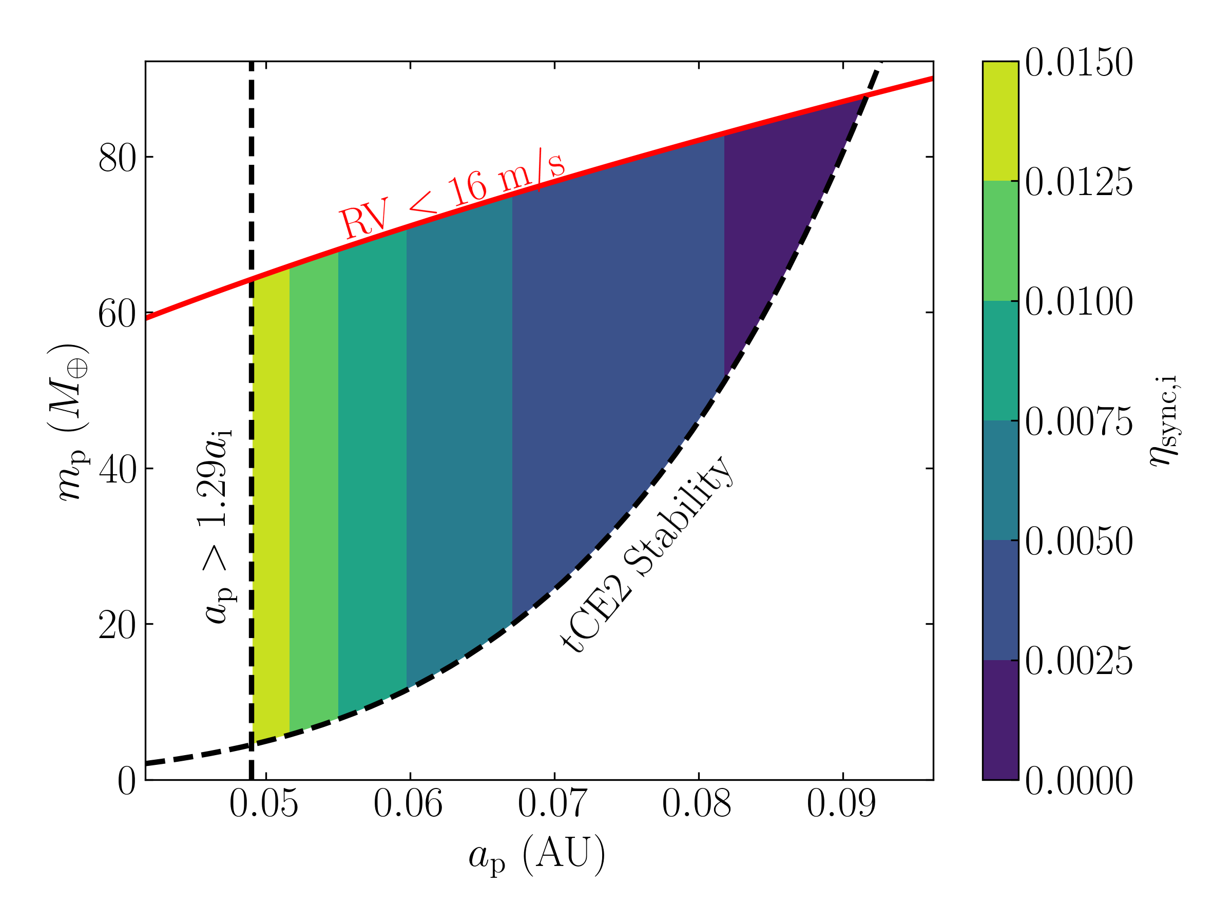
Figure 24: Constraints on the companion of WASP-12b and the values of $\eta_{\rm sync,i}$ (Eq. 61) in the obliquity tidal decay scenario. The right dashed line is from Eq. (64), required for the current system to be locked in a stable tCE2; the left vertical line is from Eq. (67), required for the dynamical stability of the “primordial” system; the red line is from Eq. (65). The probability of capture into tCE2 (starting from a isotropic distribution of spin orientation) is proportional to $\eta_{\rm sync,i}^{1/2}$ (see Eq. 47 with $I$ replaced by $I_{\rm J}$, and note that $I_{\rm J}\ll 1$ for the WASP-12b system). The plot adopts the largest possible value of $a_{\rm i}$ ($=0.038\;\mathrm{AU}>0.023\;\mathrm{AU}=a$); using a smaller $a_{\rm i}$ would significantly reduce $\eta_{\rm sync,i}$, making capture into tCE2 even less likely.

6 Summary and Discussion

We have presented a comprehensive study on the evolution of a planet’s spin (both magnitude and direction) due to the combined effects of tidal dissipation and gravitational interaction with an exterior companion/perturber. This paper extends our previous study (Su & Lai, 2020) of Colombo’s Top (“spin + companion” system) to include dissipative tidal effects, for which we have adopted the weak friction theory of the equilibrium tide. Our paper contains several new general theoretical results that can be adapted to various situations, as well as three applications to exoplanetary systems of current interest.

We summarize our general theoretical results and provide a guide to the key equations and figures as follows:

1. In the presence of a spin-orbit alignment torque (such as that arising from tidal dissipation), our linear analysis (Section 3.2) shows explicitly that only two of the equilibrium spin orientations (called “Cassini States”, CSs) are stable and attracting (see Fig. 1): the “simple” CS1 (which typically has a low obliquity) and the “resonant” CS2 (which can have a large obliquity). The latter arises from the spin-orbit resonance, which occurs when the spin precession frequency of the planet is comparable to the orbital precession frequency driven by the companion. However, when the alignment torque is too strong (or the alignment timescale $t_{\rm al}$ too short), the CSs themselves can be significantly modified. In particular, when $t_{\rm al}$ is shorter than a critical value (of order the planet’s orbital precession period; see Eq. 13), CS2 becomes destabilized and ceases to exist.

2. We compute the long-term evolution of the planetary spin obliquity driven by the alignment torque for an arbitrary initial spin orientation (Section 3.3). When neglecting the evolution of the planet’s spin magnitude, which implies that the spin and orbital precession frequencies $\alpha$, $g$ (see Eqs. 3–4) and the ratio $\eta=-g/\alpha$ are held constant, the asymptotic outcomes of the obliquity evolution (CS1 or CS2) can be analytically determined from the initial spin orientation (see Fig. 5), and we have obtained a new analytical expression for the probability of resonance capture into CS2 (Eq. 30 and Fig. 7).

3. In general, tidal torques act on both the obliquity and magnitude of the planetary spin, thus the ratio $\eta=-g/\alpha$ (which determines the phase-space structure of the system) evolves in time. Still, there are at most two equilibrium configurations (spin magnitude and obliquity) that are stable under the effect of tidal dissipation. We call these tidal Cassini Equilibria (tCE; see Fig. 8). The locations of these equilibria are determined by the system architecture and are parameterized by $\eta_{\rm sync}$ (Eq. 39), the ratio $\eta$ evaluated for $\Omega_{s}=n$ (fully synchronized spin rate).

4. We show that if tCE1 exists (which requires $\eta_{\rm sync}<\eta_{\rm c}$, where $\eta_{\rm c}$ is given by Eqs. 7; Section 4.1), which tCE a given initial planetary spin configuration asymptotically evolves towards depends on which of the phase space zones (see Fig. 2) the initial spin orientation belongs to (see Figs. 15–17): (i) If the spin originates in zone I, then it generally evolves towards tCE1 (unless $\eta_{\rm sync}$ very near $\eta_{\rm c}$, e.g. see Fig. 17); (ii) if the spin originates in zone II, then it evolves towards tCE2 (which has a nontrivial obliquity); and (iii) if the spin originates in zone III, the outcome is generally probabilistic.

5. For initial conditions in zone III, the probability of approaching either tCE can be determined by careful study of the dynamics upon separatrix encounter (Sections 3.4 and 4.3); Figs. 18 and 19 give two example results. Assuming that the initial spin orientation is isotropically distributed, we have computed the overall probability of the system evolving into tCE2 as a function of $\eta_{\rm sync}$: Figs. 20 and 21 give the results for two different planet mutual inclinations, and Eq. (47) gives an approximate analytical expression valid for $\eta_{\rm sync}\ll 1$.

Applying our general theoretical results to three types of exoplanetary systems, our key findings are (see Section 5):

1. We show that over a wide range of parameter space, a super-Earth (SE) with an exterior cold Jupiter companion (or other types of companions with a similar $m_{\rm p}/a_{\rm p}^{3}$) has a substantial probability of being trapped in a permanent tCE2 with a significant obliquity, assuming that SEs have a wide range of primordial obliquities (e.g. due to giant impacts or collisions).

2. We show that, in general, the formation of ultra-short-period planets (USPs) via runaway orbital decay driven by obliquity tides is difficult due to the low probability of capture into the high-obliquity tCE2. More importantly, proto-USPs that happen to be captured into tCE2 and initiate runaway tidal migration will likely break away from tCE2 and cease their inward migration before becoming a USP.

3. The hot Jupiter WASP-12b is unlikely to be undergoing enhanced orbital decay due to obliquity tides, as the capture into tCE2 has a low probability or requires rather special initial conditions.

Finally, we mention some possible caveats of our study. We have adopted dissipative tidal torques according to the (parameterized) weak friction theory of the equilibrium tide. Other mechanisms of tidal dissipation may be dominant, depending on the internal property of the planet and the nature of tidal forcing (e.g. Papaloizou & Ivanov, 2010; Ogilvie, 2014; Storch & Lai, 2014). We expect that, with proper parameterization and rescaling, our theoretical results presented in Sections 3–4 are largely unaffected by the details of the tidal model. In any case, a different tidal model is amenable to the same analysis as presented in this paper: The tCEs can still be found by an analysis similar to that shown in Fig. 8, and the probabilistic outcome of a separatrix encounter can still be solved using the techniques developed in Sections 3.4 and 4.3.

Some of results presented in Section 4, such as Figs. 20–22, pertain to the probabilistic outcomes of an initially isotropic distribution of spin orientations, assuming that giant impacts or planet collisions effectively randomize a planet’s primordial spin. More physically accurate distributions can be used in the case of planetary mergers (Li & Lai, 2020) or many smaller impacts (Dones & Tremaine, 1993). Figures 20–21 can be updated accordingly by convolving any initial obliquity distribution with the tCE2 capture probability distributions, such as those shown in the right panels of Figs. 15–17 or the upper panels of Figs. 18–19. The qualitative results are unlikely to change, though the detailed probabilities for tCE2 capture can increase (decrease) if the initial obliquity distribution favors (disfavors) $\theta_{\rm i}\approx 90^{\circ}$ compared to the isotropic distribution.

7 Acknowledgements

We thank the anonymous referee for their useful comments. We thank Alexandre Correia, Sarah Millholland, and Phil Nicholson for useful discussions and comments. This work has been supported in part by NSF grant AST-2107796 and NASA grant 80NSSC19K0444. YS is supported by the NASA FINESST grant 19-ASTRO19-0041.

8 Data Availability

The data referenced in this article will be shared upon reasonable request to the corresponding author.

Appendix A Convergence of Initial Conditions Inside the Separatrix to CS2

In Section 3.2, we studied the stability of the CSs under of tidal alignment torque given by Eq. (9), finding that CS2 is locally stable. Later, in Section 3.3, we found that all initial conditions within the separatrix converge to CS2, which is not guaranteed by local stability of CS2. In this section, we give an analytic demonstration that all points inside the separatrix indeed converge to CS2, focusing on the case where $\eta\ll 1$.

Similarly to the analytic calculation in Section 3.4, we seek to compute the change in the unperturbed Hamiltonian over a single libration cycle. To calculate the evolution of $H$, we first parameterize the unperturbed trajectory (similarly to Eq. 27). For initial conditions inside the separatrix, the value of $H$ can be written $H=H_{\rm sep}+\Delta H$ where $\Delta H>0$, and the two legs of the libration trajectory can be written:

$$\cos\theta_{\pm} \approx\eta\cos I\pm\sqrt{2\eta\left[\sin I\left(1-\cos\phi\right)-\Delta H\right]}.$$ (68)

We have taken $\sin\theta\approx 1$, a good approximation in zone II when $\eta\ll 1$. Note that there are some values of $\phi$ for which no solutions of $\theta$ exist, reflecting the fact that the libration cycle does not extend over the full interval $\phi\in[0,2\pi]$. During a libration cycle, $\theta_{-}$ [$\theta_{+}$] is traversed while $\phi^{\prime}>0$ [$\phi^{\prime}<0$], i.e. the trajectory librates counterclockwise in $(\cos\theta,\phi)$ phase space (see Fig. 2).

The leading order change to $H$ over a single libration cycle can then computed by integrating $\mathrm{d}H/\mathrm{d}t$ along this trajectory, yielding:

$$\oint\frac{\mathrm{d}H}{\mathrm{d}t}\;\mathrm{d}t =\oint\left(\frac{\mathrm{d}(\cos\theta)}{\mathrm{d}t}\right)_{\rm tide}\;\mathrm{d}\phi,$$

$$=\int\limits_{\phi_{\min}}^{\phi_{\max}}\frac{1}{t_{\rm s}}\left(\sin^{2}\theta_{-}-\sin^{2}\theta_{+}\right)\;\mathrm{d}\phi$$

$$\approx\frac{1}{t_{\rm s}}\int\limits_{\phi_{\min}}^{\phi_{\max}}4\eta\cos I\sqrt{2\eta\left[\sin I\left(1-\cos\phi\right)-\Delta H\right]}\;\mathrm{d}\phi>0.$$ (69)

Here, $\phi_{\min}>0$ and $\phi_{\max}<2\pi$ are defined such that the trajectory librates over $\phi\in\left[\phi_{\min},\phi_{\max}\right]$. Thus, $H$ is strictly increasing for all initial conditions inside the separatrix, and they all converge to CS2.

Appendix B Approximate TCE2 Probability for Small $\eta_{\rm sync}$

In this appendix, we seek a tentative analytic understanding for the probability of convergence to tCE2 when $\eta_{\rm sync}$ is small, i.e. the left extremes of Figs. 20 and 21. In this regime, following the discussions in Sections 3.4 and 4.3, we understand that initial conditions (ICs) in zone I always converge to tCE1, ICs in zone II always converge to tCE2, and ICs in zone III experience separatrix encounter and probabilistically converge to either one of the tCE. To further proceed, we will assume an isotropic distribution of initial spin orientations; different distributions again will only change the quantitative but not qualitative character of the discussion. Then the tCE2 probability, which we denote by $P_{\rm tCE2}$, can be expressed as the sum of: (i) the probability that an IC is in zone II, and (ii) the probability that an IC is both in zone III and undergoes a III $\to$ II transition. To simplify the discussion, we will approximate that $P_{\rm tCE2}$ can be calculated as

$$P_{\rm tCE2}\sim\frac{A_{\rm II}}{4\pi}+\frac{A_{\rm III}}{4\pi}\left\langle P_{\rm III\to II}\right\rangle,$$ (70)

where $A_{\rm II}$ and $A_{\rm III}$ are the phase space areas of zones II and III respectively, and $\left\langle P_{\rm III\to II}\right\rangle$ is the average III $\to$ II transition probability for a random IC in zone III. Next, we evaluate each of the expressions in Eq. (70).

We first consider $A_{\rm II}$ and $A_{\rm III}$. Exact analytic forms for both $A_{\rm II}$ and $A_{\rm III}$ is known (Ward & Hamilton, 2004, Paper I), but an accurate approximation can be obtained using Eq. (27) since $\eta_{\rm i}\ll 1$. We obtain that:

$$\frac{A_{\rm II}}{4\pi} =\frac{4}{\pi}\sqrt{\eta_{\rm i}\sin I},$$ (71)

$$\frac{A_{\rm III}}{4\pi} =\frac{1+\eta_{\rm i}\cos I}{2}-\frac{2}{\pi}\sqrt{\eta_{\rm i}\sin I}.$$ (72)

Next, we need to evaluate $\left\langle P_{\rm III\to II}\right\rangle$, for which we must understand the outcomes of the separatrix encounters that ICs in zone III experience. We proceed by analytically calculating $\Delta K_{\pm}$ (Eq. 45) for use in Eq. (46) to obtain the probabilities of the outcomes of separatrix encounter. We first rewrite Eq. (45) as:

$$\Delta K_{\pm} =\oint_{\mathcal{C}_{\pm}}\frac{\mathrm{d}H}{\mathrm{d}t}-\frac{\mathrm{d}H_{\rm sep}}{\mathrm{d}t}\;\mathrm{d}t$$

$$=\oint_{\mathcal{C}_{\pm}}\left(\frac{\mathrm{d}(\cos\theta)}{\mathrm{d}t}\right)_{\rm tide}+\frac{\dot{\Omega}_{\rm s}}{\dot{\phi}}\left(\frac{\partial H}{\partial\Omega_{\rm s}}-\frac{\partial H_{\rm sep}}{\partial\Omega_{\rm s}}\right)\;\mathrm{d}\phi.$$ (73)

Then, using the full equations of motion for the planet’s spin including weak tidal friction in component form, given by Eqs. (34–36), we can evaluate $\Delta K_{\pm}$ by integrating along the two legs of the separatrix $\mathcal{C}_{\pm}$ (see Fig. 2). Note that we must use the value of $\eta$ at the moment of separatrix encounter, which we denote $\eta_{\rm cross}$, as the evolution of $\Omega_{\rm s}$ changes the spin-orbit precession frequency $\alpha$ and thus $\eta$ itself:

$$t_{\rm s}\Delta K_{\pm}\approx{} \frac{\eta_{\rm cross}^{2}}{\eta_{\rm sync}}\left[-2\cos I\left(\pm 2\pi\eta_{\rm cross}\cos I+8\sqrt{\eta_{\rm cross}\sin I}\right)\mp 4\pi\sin I-8\cos I\sqrt{\eta_{\rm cross}\sin I}+\frac{4\eta_{\rm sync}}{\eta_{\rm cross}}\sqrt{\sin I/\eta_{\rm cross}}\right]$$

$$+\frac{2\eta_{\rm cross}}{\eta_{\rm sync}}\left(\mp 2\pi\left(1-2\eta_{\rm cross}\sin I\right)+16\cos I\eta_{\rm cross}^{3/2}\sqrt{\sin I}\right)+8\sqrt{\eta_{\rm cross}\sin I}\pm 2\pi\eta_{\rm cross}\cos I-\frac{64}{3}\left(\eta_{\rm cross}\sin I\right)^{3/2}.$$ (74)

The resulting $P_{\rm III\to II}$ obtained using this analytic $\Delta K_{\pm}$ in Eq. (46) is shown as the green dashed line in the top panel of Fig. 18, where it can be seen that agreement is reasonable for $\eta_{\rm cross}\lesssim 0.05$. For the purposes of this section, we drop all but the leading order terms in both the numerator and denominator of Eq. (46) and obtain:

$$P_{\rm III\to II}\simeq\frac{6\eta_{\rm sync}}{\pi}\sqrt{\frac{\sin I}{\eta_{\rm cross}}}.$$ (75)

However, $\eta_{\rm cross}$ cannot be expressed in closed form as a function of the ICs. Based on the bottom panel of Fig. 18, we make the crude approximation that $\eta_{\rm cross}$ is uniformly distributed between $\eta_{\rm i}$ and $\eta_{\rm sync}$. Note that if $\Omega_{\rm s}\simeq n$, then this approximation is invalid: since nearly anti-aligned spins ($\theta_{\rm i}\approx 180^{\circ}$) will undergo significant spin-down before tidal friction can realign the spin orientation, $\Omega_{\rm s,i}$ being too close to $n$ results in $\eta_{\rm cross}\ll\eta_{\rm sync}$. We thus obtain:

$$\left\langle P_{\rm III\to II}\right\rangle \sim\frac{1}{\eta_{\rm sync}-\eta_{\rm i}}\int\limits_{\eta_{\rm i}}^{\eta_{\rm sync}}P_{\rm III\to II}\;\mathrm{d}\eta_{\rm cross}$$

$$=\frac{12\sqrt{\eta_{\rm sync}\sin I}}{\pi\left(1+\sqrt{n/\Omega_{\rm s,i}}\right)}.$$ (76)

With this result, we can finally express Eq. (70) as:

$$P_{\rm tCE2} \simeq\frac{4\sqrt{\eta_{\rm sync}\sin I}}{\pi}\left[\sqrt{n/\Omega_{\rm s,i}}+\frac{3}{2\left(1+\sqrt{n/\Omega_{\rm s,i}}\right)}\right]+\mathcal{O}\left(\eta_{\rm sync}\right).$$ (77)

This is exactly Eq. (47). We remark again that this is valid in the regime where $\eta_{\rm sync}\ll 1$ and $\Omega_{\rm s}\gtrsim n$.

References

- Adams et al. (2019) Adams, A. D., Millholland, S., & Laughlin, G. P. 2019, arXiv preprint arXiv:1906.07615
- Alexander (1973) Alexander, M. 1973, Astrophysics and Space Science, 23, 459
- Anderson & Lai (2018) Anderson, K. R., & Lai, D. 2018, Monthly Notices of the Royal Astronomical Society, 480, 1402
- Barker (2020) Barker, A. J. 2020, Monthly Notices of the Royal Astronomical Society, 498, 2270
- Benz et al. (1989) Benz, W., Slattery, W., & Cameron, A. 1989, Meteoritics, 24, 251
- Bonomo et al. (2017) Bonomo, A. S., Desidera, S., Benatti, S., et al. 2017, Astronomy & Astrophysics, 602, A107
- Bryan et al. (2018) Bryan, M. L., Benneke, B., Knutson, H. A., Batygin, K., & Bowler, B. P. 2018, Nature Astronomy, 2, 138
- Bryan et al. (2019) Bryan, M. L., Knutson, H. A., Lee, E. J., et al. 2019, The Astronomical Journal, 157, 52
- Bryan et al. (2020) Bryan, M. L., Chiang, E., Bowler, B. P., et al. 2020, The Astronomical Journal, 159, 181
- Colombo (1966) Colombo, G. 1966, The Astronomical Journal, 71, 891
- Dai et al. (2018) Dai, F., Masuda, K., & Winn, J. N. 2018, The Astrophysical Journal Letters, 864, L38
- Dones & Tremaine (1993) Dones, L., & Tremaine, S. 1993, Science, 259, 350
- Fabrycky et al. (2007) Fabrycky, D. C., Johnson, E. T., & Goodman, J. 2007, The Astrophysical Journal, 665, 754
- Fabrycky et al. (2014) Fabrycky, D. C., Lissauer, J. J., Ragozzine, D., et al. 2014, The Astrophysical Journal, 790, 146
- Fricke (1977) Fricke, W. 1977, Transactions of the International Astronomical Union, Series B, 16, 56
- Gladman (1993) Gladman, B. 1993, Icarus, 106, 247
- Goldreich & Peale (1966) Goldreich, P., & Peale, S. 1966, The Astronomical Journal, 71, 425
- Groten (2004) Groten, E. 2004, Journal of Geodesy, 77, 724, doi: 10.1007/s00190-003-0373-y
- Guckenheimer & Holmes (1983) Guckenheimer, J., & Holmes, P. J. 1983, Nonlinear oscillations, dynamical systems, and bifurcations of vector fields (New York: Springer-Verlag)
- Hamilton & Ward (2004) Hamilton, D. P., & Ward, W. R. 2004, The Astronomical Journal, 128, 2510
- Hebb et al. (2009) Hebb, L., Collier-Cameron, A., Loeillet, B., et al. 2009, The Astrophysical Journal, 693, 1920
- Henrard (1982) Henrard, J. 1982, Celestial Mechanics and Dynamical Astronomy, 27, 3
- Henrard & Murigande (1987) Henrard, J., & Murigande, C. 1987, Celestial Mechanics, 40, 345
- Husnoo et al. (2011) Husnoo, N., Pont, F., Hébrard, G., et al. 2011, Monthly Notices of the Royal Astronomical Society, 413, 2500
- Hut (1981) Hut, P. 1981, Astronomy and Astrophysics, 99, 126
- Inamdar & Schlichting (2015) Inamdar, N. K., & Schlichting, H. E. 2015, Monthly Notices of the Royal Astronomical Society, 448, 1751
- Izidoro et al. (2017) Izidoro, A., Ogihara, M., Raymond, S. N., et al. 2017, Monthly Notices of the Royal Astronomical Society, 470, 1750
- Knutson et al. (2014) Knutson, H. A., Fulton, B. J., Montet, B. T., et al. 2014, The Astrophysical Journal, 785, 126
- Korycansky et al. (1990) Korycansky, D., Bodenheimer, P., Cassen, P., & Pollack, J. 1990, Icarus, 84, 528
- Lai (2012) Lai, D. 2012, Monthly Notices of the Royal Astronomical Society, 423, 486
- Lai & Pu (2017) Lai, D., & Pu, B. 2017, The Astronomical Journal, 153, 42, doi: 10.3847/1538-3881/153/1/42
- Lainey (2016) Lainey, V. 2016, Celestial Mechanics and Dynamical Astronomy, 126, 145
- Lee & Chiang (2017) Lee, E. J., & Chiang, E. 2017, The Astrophysical Journal, 842, 40
- Levrard et al. (2007) Levrard, B., Correia, A., Chabrier, G., et al. 2007, Astronomy & Astrophysics, 462, L5
- Li & Lai (2020) Li, J., & Lai, D. 2020, The Astrophysical Journal Letters, 898, L20
- Li et al. (2021) Li, J., Lai, D., Anderson, K. R., & Pu, B. 2021, Monthly Notices of the Royal Astronomical Society, 501, 1621
- Maciejewski et al. (2013) Maciejewski, G., Dimitrov, D., Seeliger, M., et al. 2013, Astronomy & Astrophysics, 551, A108
- Maciejewski et al. (2016) Maciejewski, G., Dimitrov, D., Fernández, M., et al. 2016, Astronomy & Astrophysics, 588, L6
- Millholland & Batygin (2019) Millholland, S., & Batygin, K. 2019, The Astrophysical Journal, 876, 119