Inverse seesaw in $A_{5}^{\prime}$ modular symmetry

Abstract

We make an investigation of modular $\Gamma^{\prime}_{5}\simeq A^{\prime}_{5}$ group in inverse seesaw framework. Modular symmetry is advantageous because it reduces the usage of extra scalar fields significantly. Moreover, the Yukawa couplings are expressed in terms of Dedekind eta functions, which also have a $q$ expansion form, utilized to achieve numerical simplicity. Our proposed model includes six heavy fermion superfields i.e., $\mathcal{N}_{Ri}$, $\mathcal{S}_{Li}$ and a weighton. The study of neutrino phenomenology becomes simplified and effective by the usage of $A^{\prime}_{5}$ modular symmetry, which provides us a well defined mass structure for the lepton sector. Here, we observe that all the neutrino oscillation parameters, as well as the effective electron neutrino mass in neutrinoless double beta decay can be accommodated in this model. We also briefly discuss the lepton flavor violating decays $\ell_{i}\to\ell_{j}\gamma$ and comment on non-unitarity of lepton mixing matrix.

I INTRODUCTION

The results from various neutrino oscillation experiments have unambiguously established the fact that neutrinos posses very small but non-zero masses contradicting their vanishing mass concept presumed in the Standard Model (SM). Therefore, understanding the origin of the neutrino mass necessitates to employ physics beyond the SM. One of the conventional ways to generate the light neutrino masses is through the canonical seesaw mechanism Mohapatra:1979ia ; Brdar:2019iem ; Branco:2019avf ; Bilenky:2010zza , where three heavy right handed (RH) neutrinos $\mathcal{N}_{R_{i}}$ are introduced on top of the SM particle spectrum. The inclusion of right-handed neutrinos not only generates the Dirac mass term but also leads to Majorana mass for $\mathcal{N}_{Ri}$’s, of the form $\overline{\mathcal{N}_{Ri}}\mathcal{N}_{Ri}^{c}$ which violates the lepton number by two units. The master formula for generating the masses of the active neutrinos is governed by $m_{\nu}\approx-\mathcal{M}_{D}\mathcal{M}^{-1}_{R}\mathcal{M}^{T}_{D}$, where $\mathcal{M}_{D}$ is the Dirac neutrino mass matrix and $\mathcal{M}_{R}$ being the Majorana neutrino mass matrix of the heavy RH neutrinos, satisfying the relation $\mathcal{M}_{D}$ $\ll\mathcal{M}_{R}$. However, myriad literature on seesaw models show work on other extensions like type-II, with the inclusion of a scalar triplet Gu:2006wj ; Luo:2007mq ; Antusch:2004xy ; Rodejohann:2004cg ; Gu:2019ogb ; McDonald:2007ka , type-III Liao:2009nq ; Ma:1998dn ; Foot:1988aq ; Dorsner:2006fx ; Franceschini:2008pz ; He:2009tf , where a fermion triplet is added to the SM particle content. In these approaches, the masses of the new heavy particles are quite heavy and are beyond the access of the present and future experiments.

Many other alternative approaches were proposed, e.g., linear seesaw Ma:2009du ; Gu:2010xc ; Sruthilaya:2017mzt ; Borah:2018nvu , inverse seesaw Das:2012ze ; Arganda:2014dta ; Ma:2015raa ; Dias:2012xp ; Dev:2012sg ; Dias:2011sq ; Bazzocchi:2010dt , where the new physics scale responsible for neutrino mass generation can be brought down to TeV scale, at the expense of the inclusion of new additional fermion fields ($S_{i}$), which are SM singlets. The inverse seesaw formalism is implemented by including three additional left handed (LH) singlet fermions $\mathcal{S}_{L_{i}}$ and hence, the basis that involves for the neutrino mass generation is $(\nu_{L}^{c},\mathcal{N}_{R_{i}},\mathcal{S}_{L_{i}})^{T}$. This leads to the neutrino mass matrix structure as $m_{\nu}\approx(\mathcal{M}_{D}/\mathcal{M}_{RS})~{}\mathcal{M}_{\mu}~{}(\mathcal{M}_{D}/\mathcal{M}_{RS})^{T}$, where $\mathcal{M}_{\mu}$ is the Majorana mass term for the heavy singlet fermion $S_{Li}$. For inverse seesaw, the various mass terms satisfy the relation $\mathcal{M}_{\mu}\ll\mathcal{M}_{D}<\mathcal{M}_{RS}$, and hence, the neutrino mass is given by $m_{\nu}\approx$ $\mathcal{M}_{D}^{2}\mathcal{M}_{\mu}/\mathcal{M}_{RS}^{2}$. So to get the correct order of the light neutrino masses, the typical values of different mass scales are: $\mathcal{M}_{D}\sim$ 10 GeV, $\mathcal{M}_{RS}\sim 10~{}\rm{TeV}$, and $\mathcal{M}_{\mu}\sim 1~{}\rm{keV}$.

Genearally, to implement inverse seesaw certain symmtries are assumed, like discrete flavour symmetries $S_{3}$ CarcamoHernandez:2013krw ; Ma:2014qra , $A_{4}$ CarcamoHernandez:2017kra ; Borah:2017dmk ; Hirsch:2009mx ; Kalita:2015jaa ; Altarelli:2010gt , $S_{4}$ Ma:2005pd ; Dorame:2012zv ; CarcamoHernandez:2019eme etc., to avoid certain unwanted terms in the extended neutrino mass matrix of $(\nu_{L}^{c},\mathcal{N}_{R_{i}},\mathcal{S}_{L_{i}})^{T}$ basis. However, a number of flavon fields are required for the breaking of these flavor symmetries as well as to accommodate the observed neutrino oscillation data and the vacuum alignment of these flavon fields pose a challenging task. But in recent times, modular symmetry Kobayashi:2018vbk ; Feruglio:2017spp ; deAdelhartToorop:2011re has gained pace and is in the limelight. Modular symmetry removes the usage of excess flavon fields, where, the role of flavons is performed by Yukawa couplings, which are holomorphic function of modulus $\tau$. When this modulus acquires the vacuum expectation value (VEV), it breaks the flavor symmetry. Exploration of myriad text shows work on modular groups $S_{3}$ Du:2020ylx ; Mishra:2020gxg ; Okada:2019xqk , $S_{4}$ Penedo:2018nmg ; Novichkov:2018ovf ; Okada:2019lzv , $A_{4}$ Abbas:2020vuy ; Nagao:2020snm ; Asaka:2020tmo ; Nomura:2020opk ; Okada:2020dmb ; Behera:2020lpd ; Behera:2020sfe ; Ding:2019zxk ; Altarelli:2005yx , $A_{5}$ Novichkov:2018nkm ; Yao:2020zml , double covering of $A_{4}$ Liu:2019khw , double covering of $A_{5}$ Wang:2020lxk . These modular groups help to accurately calculate the neutrino oscillation parameters at $3\sigma$ level along with other observables.

In this work, we intend to focus on the double covering modular group $\Gamma^{\prime}_{5}\simeq A^{\prime}_{5}$ and its implications on neutrino phenomenology. In the past, quite a few works in the literature have been discussed the significace of finite groups, which comprehend the basic properties of $A^{\prime}_{5}$ group  Everett:2010rd ; Hashimoto:2011tn ; Chen:2011dn . So here, we mention only the essential points regarding $A^{\prime}_{5}$ modular symmetry group. The $A^{\prime}_{5}$ group has 120 elements, which can be constructed by three generators $S$, $T$ and $R$, which satisy the identities $S^{2}=R$, $(ST)^{3}=\mathbb{I}$, $R^{2}=\mathbb{I}$ and $RT=TR$ Wang:2020lxk . These 120 elements are categorized into nine conjugacy classes, which classifies them as the nine distinct irreducible representations, symbolized as ${\bf 1}$, $\widehat{\bf 2}$, $\widehat{\bf 2}^{\prime}$, ${\bf 3}$, ${\bf 3}^{\prime}$, ${\bf 4}$, $\widehat{\bf 4}$, ${\bf 5}$ and $\widehat{\bf 6}$ by their dimensions. Moreover, conjugacy classes and character table of $A^{\prime}_{5}$, as well as the representation matrices of all three generators $S$, $T$ and $R$ in the irreducible representations, are presented in Appendix Wang:2020lxk . It should be noted that the ${\bf 1}$, ${\bf 3}$, ${\bf 3}^{\prime}$, ${\bf 4}$ and ${\bf 5}$ representations with $R=\mathbb{I}$ coincide with those for $A_{5}$, whereas $\widehat{\bf 2}$, $\widehat{\bf 2}^{\prime}$, $\widehat{\bf 4}$ and $\widehat{\bf 6}$ are unique for $A^{\prime}_{5}$ with $R=-\mathbb{I}$. As we are working in the modular space of $\Gamma(5)$, hence, its dimension is $5k+1$, where, $k$ is the modular weight. A brief discussion concerning the modular space of $\Gamma(5)$ is presented in Appendix A. For $k=1$, the modular space $M_{1}[\Gamma(5)]$ will have six basis vectors i.e ($\widehat{e}_{i}$, where $i=1,2,3,4,5,6$) whose $q$-expansion is given below and they are used in expressing the Yukawa coupling $Y^{(1)}_{\widehat{\bf 6}}$ as shown in Appendix C:

$$\widehat{e}_{1} = 1+3q+4q^{2}+2q^{3}+q^{4}+3q^{5}+6q^{6}+4q^{7}-q^{9}+\cdots\;,$$

$$\widehat{e}_{2} = q^{1/5}\left(1+2q+2q^{2}+q^{3}+2q^{4}+2q^{5}+2q^{6}+q^{7}+2q^{8}+2q^{9}+\cdots\right)\;,$$

$$\widehat{e}_{3} = q^{2/5}\left(1+q+q^{2}+q^{3}+2q^{4}+q^{6}+q^{7}+2q^{8}+q^{9}+\cdots\right)\;,$$

$$\widehat{e}_{4} = q^{3/5}\left(1+q^{2}+q^{3}+q^{4}-q^{5}+2q^{6}+2q^{8}+q^{9}+\cdots\right)\;,$$

$$\widehat{e}_{5} = q^{4/5}\left(1-q+2q^{2}+2q^{6}-2q^{7}+2q^{8}+q^{9}+\cdots\right)\;,$$

$$\widehat{e}_{6} = q\left(1-2q+4q^{2}-3q^{3}+q^{4}+2q^{5}-2q^{6}+3q^{8}-2q^{9}+\cdots\right)\;.$$ (1)

Structure of this paper is as follows. In Sec. II, we discuss the model framework for generating the light neutrino masses using inverse seesaw mechanism with discrete $A^{\prime}_{5}$ modular flavor symmetry. This $A^{\prime}_{5}$ modular symmetry is double covered hence, there are more number of irreducible representation as compared to $A_{5}$ modular symmetry. This helps us to construct charged leptons and neutral lepton mass matrices. In Sec. III, numerical correlational study between the observables of neutrino sector and the model input parameters is established. A brief discussion on the non-unitarity effect is presented in Sec. IV. In addition, lepton flavor violation (LFV) in the context of the present model is presented in Sec. V and in Sec. VI, we conclude our results.

II MODEL FRAMEWORK

We consider a scenario in which inverse seesaw is implemented in the context of supersymmetry (SUSY) to study the neutrino phenomenology, where the SM is extended with a discrete $A^{\prime}_{5}$ modular symmetry. An additional local $U(1)_{B-L}$ symmetry is added to prohibit certain undesirable terms in the superpotential. The SM particle spectrum is supplemented with three extra RH singlet fermion superfields ($\mathcal{N}_{R_{i}}$), three LH singlet fermion superfields ($\mathcal{S}_{L_{i}}$) and one weighton ($\zeta$). The added fermion superfields of the model transform as $3^{\prime}$ under the $A^{\prime}_{5}$ modular group, whereas, the $U(1)_{B-L}$ charges assigned to them are $-1$ ($\mathcal{N}_{R_{i}}$) and 0 ($\mathcal{S}_{L_{i}}$). Also RH neutrinos are assigned modular weight 6 and LH neutrinos with 0. The particle content and their charges under various groups are provided in Table 1. The $A^{\prime}_{5}$ and $U(1)_{B-L}$ symmetries are considered to be broken at a scale much higher than the electroweak symmetry breaking Dawson:2017ksx . The $U(1)_{B-L}$ symmetry is spontaneously broken by assigning non-zero vacuum expectation value (VEV) to the singlet weighton $\zeta$, and consequently the additional singlet fermion superfields acquire their masses. In addition to above, several higher order Yukawa couplings are introduced which obey the rule: $k_{Y}=k_{I_{1}}+k_{I_{2}}+\cdots+k_{I_{n}}$, where $k_{Y}$ is the weight on the Yukawa couplings and $k_{I_{i}}(i=1,2,3,4\cdots)$ are the weights on the superfields. These higher order Yukawa couplings implicitly depend on $Y^{(1)}_{\widehat{\bf 6}}$ whose complete forms are shown in Appendix C.

Fields	$e_{R}$	$\mu_{R}$	$\tau_{R}$	$\overline{L}_{L}$	$\mathcal{N}_{R}$	$\mathcal{S}_{L}$	$\mathcal{H}_{u,d}$	$\zeta$
$SU(2)_{L}$	$1$	$1$	$1$	$2$	$1$	$1$	$2$	$1$
$U(1)_{Y}$	$1$	$1$	$1$	$-\frac{1}{2}$	$0$	$0$	$\frac{1}{2},-\frac{1}{2}$	$0$
$A_{5}^{\prime}$	$1$	$1$	$1$	$3$	$3^{\prime}$	$3^{\prime}$	$1$	$1$
$U(1)_{B-L}$	$-1$	$-1$	$-1$	$1$	$-1$	$0$	$0$	$1$
$k_{I}$	$2$	$4$	$6$	$0$	$6$	$0$	$0$	$0$

Table 1: Particle content of the model and their charges under $SU(2)_{L}\times U(1)_{Y}\times A_{5}^{\prime}\times U_{B-L}$ group and their modular weights $k_{I}$.

The superpotential of the model is given by

$$\mathcal{W} = A_{\mathcal{M}_{l}}\left[(\overline{L}_{L}l_{R}))_{\textbf{3}}Y^{k_{I}}_{\textbf{3}}\right]\mathcal{H}_{d}+\mu\mathcal{H}_{u}\mathcal{H}_{d}+G_{D}\Big{[}(\overline{L}_{L}\mathcal{N}_{R}))_{\textbf{4}}\sum\limits^{2}_{i=1}Y_{\textbf{4},i}^{(6)}\Big{]}\mathcal{H}_{u}$$

$$+ B_{\mathcal{M}_{RS}}\Big{[}(\overline{\mathcal{S}}_{L}\mathcal{N}_{R})_{\bf 5}\sum\limits^{2}_{i=1}Y_{\textbf{5},i}^{(6)}\Big{]}\zeta+\mu_{0}\overline{S^{C}_{L}}S_{L}\;,$$

where, $A_{\mathcal{M}_{l}}$, $G_{D}$ and $B_{\mathcal{M}_{RS}}$ are $3\times 3$ diagonal matrices given as $A_{\mathcal{M}_{l}}={\rm diag}\left(\alpha_{\mathcal{M}_{l}},\beta_{\mathcal{M}_{l}},\gamma_{\mathcal{M}_{l}}\right)$, $G_{D}={\rm diag}\left(g_{D_{1}},g_{D_{2}},g_{D_{3}}\right)$, and $B_{\mathcal{M}_{RS}}={\rm diag}\left(\alpha_{RS_{1}},\alpha_{RS_{2}},\alpha_{RS_{3}}\right)$. The modular weight $k_{I}$ in the first term takes the values $k_{I}=(2,4,6)$ for $l=(e,\mu,\tau)$.

II.1 Dirac mass term for charged leptons

To establish charged leptons mass matrix, the left-handed doublet superfields i.e., $\overline{L}_{L}$, transform as triplets under the $A^{\prime}_{5}$ symmetry with $B-L$ charge $-1$. The Higgsinos $\mathcal{H}_{u,d}$ are given charges 0, 1 under the $U_{B-L}$ and $A^{\prime}_{5}$ symmetries respectively with zero modular weight. The VEVs of these Higgsinos $\mathcal{H}_{u}$ and $\mathcal{H}_{d}$ are given as $v_{u}/\sqrt{2}$ and $v_{d}/\sqrt{2}$ respectively. Moreover, Higgsinos VEVs are associated to SM Higgs VEV as $v_{H}=\frac{1}{2}\sqrt{v^{2}_{u}+v^{2}_{d}}$ and the ratio of their VEVs is expressed as $\tan\beta=({v_{u}}/{v_{d}})=5$. Hence, the relevant superpotential term for charged leptons is given as

$$\mathcal{W}_{\mathcal{M}_{l}} =\alpha_{\mathcal{M}_{l}}\left[(\overline{L_{L}}e_{R})_{\bf 3}Y_{\bf{3}}^{(2)}\right]\mathcal{H}_{d}+\beta_{\mathcal{M}_{l}}\left[(\overline{L_{L}}\mu_{R})_{\bf{3}}Y_{\bf{3}}^{(4)}\right]\mathcal{H}_{d}+\gamma_{\mathcal{M}_{l}}\Big{[}(\overline{L_{L}}\tau_{R})_{\bf{3}}\Big{\{}\sum\limits_{i=1}^{2}Y_{{\bf{3}},i}^{(6)}\Big{\}}\Big{]}\mathcal{H}_{d}\;.$$ (3)

After the spontaneous symmetry breaking, it is evident that the charged lepton mass matrix isn’t diagonal and is expressed as

$$\mathcal{M}_{l} =\frac{v_{d}}{\sqrt{6}}\left[\begin{matrix}\left(Y^{(2)}_{\bf 3}\right)_{1}&&\left(Y^{(4)}_{\bf 3}\right)_{1}&&\left(\sum\limits_{i=1}^{2}Y^{(6)}_{{\bf 3},i}\right)_{1}\\ \left(Y^{(2)}_{\bf 3}\right)_{3}&&\left(Y^{(4)}_{\bf 3}\right)_{3}&&\left(\sum\limits_{i=1}^{2}Y^{(6)}_{{\bf 3},i}\right)_{3}\\ \left(Y^{(2)}_{\bf 3}\right)_{2}&&\left(Y^{(4)}_{\bf 3}\right)_{2}&&\left(\sum\limits_{i=1}^{2}Y^{(6)}_{{\bf 3},i}\right)_{2}\\ \end{matrix}\right]_{LR}\cdot\left[\begin{array}[]{ccc}\alpha_{\mathcal{M}_{l}}&0&0\\ 0&\beta_{\mathcal{M}_{l}}&0\\ 0&0&\gamma_{\mathcal{M}_{l}}\\ \end{array}\right]\;.$$ (7)

The charged lepton mass matrix ${\mathcal{M}}_{l}$ can be diagonalised by the unitary matrix $U_{l}$, giving rise to the physical masses $e,~{}\mu$ and $\tau$ as

$$U^{\dagger}_{l}\mathcal{M}_{l}\mathcal{M}^{\dagger}_{l}U_{l}={\rm diag}(m^{2}_{e},m^{2}_{\mu},m^{2}_{\tau})\;.$$ (8)

In addition, it also satisfies the following identities, which will be used for numerical analysis in section III:

$${\rm Tr}\left(\mathcal{M}_{l}\mathcal{M}^{{\dagger}}_{l}\right) = m^{2}_{e}+m^{2}_{\mu}+m^{2}_{\tau}\;,$$

$${\rm Det}\left(\mathcal{M}_{l}\mathcal{M}^{{\dagger}}_{l}\right) = m^{2}_{e}m^{2}_{\mu}m^{2}_{\tau}\;,$$

$$\dfrac{1}{2}\left[{\rm Tr}\left(\mathcal{M}_{l}\mathcal{M}^{{\dagger}}_{l}\right)\right]^{2}-\dfrac{1}{2}{\rm Tr}\left[(\mathcal{M}_{l}\mathcal{M}^{{\dagger}}_{l})^{2}\right] = m^{2}_{e}m^{2}_{\mu}+m^{2}_{\mu}m^{2}_{\tau}+m^{2}_{\tau}m^{2}_{e}\;.$$ (9)

II.2 Dirac mass term for neutrinos

The right-handed neutrino superfields ${\cal N}_{R_{i}}$ are $\bm{3^{\prime}}$ under $A^{\prime}_{5}$ modular group with a ${B-L}$ charge of $-1$ and modular weight $6$. Therefore, the invariant superpotential, describing the Dirac mass term for the neutrinos can be written as,

$$\mathcal{W}_{D} =G_{D}\left[(\overline{L}_{L}~{}\mathcal{N}_{R})_{\textbf{4}}\sum\limits^{2}_{i=1}Y_{\textbf{4},i}^{(6)}\right]\mathcal{H}_{u}\;.$$ (10)

Here, the subscript for the operator $\overline{L}_{L}\mathcal{N}_{R}$ indicates $A^{\prime}_{5}$ representation constructed by the Kronecker product rule (see Appendix B) which further leads in obtaining a invariant superpotential. The resulting Dirac neutrino mass matrix is found to be

$$\mathcal{M}_{D} =\frac{v_{u}}{2\sqrt{6}}\left[\begin{array}[]{ccc}0&-\sqrt{2}\left(\sum\limits^{2}_{i=1}Y_{\textbf{4},i}^{(6)}\right)_{{3}}&-\sqrt{2}\left(\sum\limits^{2}_{i=1}Y_{\textbf{4},i}^{(6)}\right)_{{2}}\vspace{2mm}\\ \sqrt{2}\left(\sum\limits^{2}_{i=1}Y_{\textbf{4},i}^{(6)}\right)_{{4}}&\left(\sum\limits^{2}_{i=1}Y_{\textbf{4},i}^{(6)}\right)_{{2}}&-\sqrt{2}\left(\sum\limits^{2}_{i=1}Y_{\textbf{4},i}^{(6)}\right)_{{1}}\vspace{2mm}\\ \sqrt{2}\left(\sum\limits^{2}_{i=1}Y_{\textbf{4},i}^{(6)}\right)_{{1}}&\left(\sum\limits^{2}_{i=1}Y_{\textbf{4},i}^{(6)}\right)_{{4}}&-\left(\sum\limits^{2}_{i=1}Y_{\textbf{4},i}^{(6)}\right)_{{3}}\\ \end{array}\right]_{LR}.\begin{bmatrix}g_{D_{1}}&0&0\\ 0&g_{D_{2}}&0\\ 0&0&g_{D_{3}}\end{bmatrix}\;,$$ (14)

where $(g_{D_{1}},g_{D_{2}},g_{D_{3}})$ are the free parameters of the diagonal matrix $G_{D}$.

II.3 Mixing between the heavy fermions $\mathcal{N}_{R}$ and $\mathcal{S}_{L}$

The mixing between heavy fermion superfields ${\cal N}_{R}$ and ${\cal S}_{L}$ can be expressed as follows,

$$\mathcal{W}_{\mathcal{M}_{RS}} = B_{\mathcal{M}_{RS}}\Big{[}(\overline{\mathcal{S}}_{L}\mathcal{N}_{R})_{\bf 5}\sum\limits^{2}_{i=1}Y_{\bf 5,i}^{(6)}\Big{]}\zeta$$ (15)

where, the choice of Yukawa coupling depends on the sum of the modular weight of the superfields and the Kronecker product rule as given in Appendix B. Using $\langle\zeta\rangle=v_{\zeta}/\sqrt{2}$, the resulting mass matrix is found to be

$$\mathcal{M}_{RS} =\frac{v_{\zeta}}{2\sqrt{1}5}\left[\begin{array}[]{ccc}2\left(\sum\limits_{i=1}^{2}Y_{\textbf{5,i}}^{(6)}\right)_{1}&-\sqrt{3}\left(\sum\limits_{i=1}^{2}Y_{\textbf{5,i}}^{(6)}\right)_{4}&-\sqrt{3}\left(\sum\limits_{i=1}^{2}Y_{\textbf{5,i}}^{(6)}\right)_{3}\\ -\sqrt{3}\left(\sum\limits_{i=1}^{2}Y_{\textbf{5,i}}^{(6)}\right)_{4}&-\sqrt{6}\left(\sum\limits_{i=1}^{2}Y_{\textbf{5,i}}^{(6)}\right)_{2}&-\left(\sum\limits_{i=1}^{2}Y_{\textbf{5,i}}^{(6)}\right)_{1}\\ -\sqrt{3}\left(\sum\limits_{i=1}^{2}Y_{\textbf{5,i}}^{(6)}\right)_{3}&-\left(\sum\limits_{i=1}^{2}Y_{\textbf{5,i}}^{(6)}\right)_{1}&-\sqrt{6}\left(\sum\limits_{i=1}^{2}Y_{\textbf{5,i}}^{(6)}\right)_{5}\\ \end{array}\right]_{LR}.\begin{bmatrix}\alpha_{RS_{1}}&0&0\\ 0&\alpha_{RS_{2}}&0\\ 0&0&\alpha_{RS_{3}}\end{bmatrix}\;,$$ (19)

where $(\alpha_{RS_{1}},\alpha_{RS_{2}},\alpha_{RS_{3}})$ are the free paramaters of the diagonal matrix $B_{\mathcal{M}_{RS}}$.

II.4 Majorana mass term for $\mathcal{S}_{L}$

Under $A^{\prime}_{5}$ singlet heavy fermions ${\cal S}_{L}$ transform as triplet $\bm{3^{\prime}}$ having zero modular weight. Hence, its Majorana mass term can be written as,

$$\mathcal{W}_{\mu} =\mu_{0}\mathcal{S}_{L}\mathcal{S}_{L},$$ (20)

leading to the mass matrix ($\mathcal{M}_{\mu}$) of the form

$$\mathcal{M}_{\mu}=\mu_{0}\begin{bmatrix}1&0&0\\ 0&0&1\\ 0&1&0\end{bmatrix}.$$ (21)

II.5 Inverse Seesaw mechanism for light neutrino Masses

In the present model constructed using $A^{\prime}_{5}$ modular symmetry, the complete $9\times 9$ neutral fermion mass matrix in the flavor basis of $\left(\nu_{L},{\cal N}_{R},{\cal S}^{c}_{L}\right)^{T}$ is given as

$$\mathbb{M}=\left(\begin{array}[]{c|ccc}&\nu_{L}&\mathcal{N}_{R}&\mathcal{S}^{c}_{L}\\ \hline\cr\nu_{L}&0&\mathcal{M}_{D}&0\\ \mathcal{N}_{R}&\mathcal{M}^{T}_{D}&0&\mathcal{M}_{RS}\\ \mathcal{S}^{c}_{L}&0&\mathcal{M}_{RS}^{T}&\mathcal{M}_{\mu}\end{array}\right).$$ (26)

In the limit $\mathcal{M}_{\mu}\ll M_{D}<M_{RS}$, the above mass matrix (26) provides the inverse seesaw mass formula for the light neutrinos as

$$m_{\nu} = \mathcal{M}_{D}~{}\mathcal{M}_{RS}^{-1}~{}\mathcal{M}_{\mu}~{}(\mathcal{M}_{RS}^{-1})^{T}~{}(\mathcal{M}_{D})^{T}.$$ (27)

Thus, diagonalization of the light neutrino mass matrix (27) yields the masses of the active neutrinos. Apart from determining the small neutrino masses, other parameters, which are of great use, are the Jarlskog invariant ($J_{CP}$) and the effective neutrino mass $\langle m_{ee}\rangle$ describing the neutrinoless double beta decay. These parameters related to the mixing angles and phases of PMNS matrix through

$$J_{CP}=\text{Im}[U_{e1}U_{\mu 2}U_{e2}^{*}U_{\mu 1}^{*}]=s_{23}c_{23}s_{12}c_{12}s_{13}c^{2}_{13}\sin\delta_{CP}\;,$$ (28)

$$\langle m_{ee}\rangle=|m_{\nu_{1}}\cos^{2}\theta_{12}\cos^{2}\theta_{13}+m_{\nu_{2}}\sin^{2}\theta_{12}\cos^{2}\theta_{13}e^{i\alpha_{21}}+m_{\nu_{3}}\sin^{2}\theta_{13}e^{i(\alpha_{31}-2\delta_{CP})}|.$$ (29)

The effective Majorana mass parameter $\langle m_{ee}\rangle$ is expected to have improved sensitivity measured by KamLAND-Zen experiment in coming future KamLAND-Zen:2016pfg .

III NUMERICAL ANALYSIS

Numerical analysis is performed by considering experimental data at 3$\sigma$ interval deSalas:2020pgw as follows:

$${\rm NO}:\Delta m^{2}_{\rm atm}=[2.47,2.63]\times 10^{-3}\ {\rm eV}^{2},\ \Delta m^{2}_{\rm sol}=[6.94,8.14]\times 10^{-5}\ {\rm eV}^{2},$$

$$\sin^{2}\theta_{13}=[0.0200,0.02405],\ \sin^{2}\theta_{23}=[0.434,0.610],\ \sin^{2}\theta_{12}=[0.271,0.369]\;.$$ (30)

Here, numerical diagonalization of the light neutrino mass matrix as given in eqn.(27) is done through $U_{\nu}^{\dagger}{\cal M}U_{\nu}={\rm diag}(m_{1}^{2},m_{2}^{2},m_{3}^{2})$, where ${\cal M}=m_{\nu}m_{\nu}^{\dagger}$ and $U_{\nu}$ is an unitary matrix. Thus, the lepton mixing matrix is given as $U=U_{l}^{\dagger}U_{\nu}$, from which the neutrino mixing angles can be extracted using the standard relations:

$$\sin^{2}\theta_{13}=|U_{13}|^{2}\;,~{}~{}~{}~{}\sin^{2}\theta_{12}=\frac{|U_{12}|^{2}}{1-|U_{13}|^{2}}\;,~{}~{}~{}~{}~{}\sin^{2}\theta_{23}=\frac{|U_{23}|^{2}}{1-|U_{13}|^{2}}\;.$$ (31)

In order to demonstrate the current neutrino oscillation data, the values of model parameters are chosen to be in the following ranges:

$${\rm Re}[\tau]\in[0,0.5],~{}~{}{\rm Im}[\tau]\in[0.5,2],~{}~{}\{g_{D_{1}},g_{D_{2}},g_{D_{3}}\}\in~{}[10^{-4},10^{-2}],$$

$$\{\alpha_{RS_{1}},\alpha_{RS_{2}},\alpha_{RS_{3}}\}\in[0.1,1],\quad v_{\zeta}\in[1,100]\ {\rm TeV}\;.$$

For diagonalizing the charged lepton mass matrix ${\mathcal{M}}_{l}$ (14), we use the values of the free parameters as: $\alpha_{\mathcal{M}_{l}}\approx\mathcal{O}(10^{-6})$, $\beta_{\mathcal{M}_{l}}\approx\mathcal{O}(10^{-2})$ and $\gamma_{\mathcal{M}_{l}}\approx\mathcal{O}(10^{-4})$, and scanning over the the allowed ranges of real and imaginary parts of the modulus $\tau$, i.e., 0 $\lesssim\$Re$[\tau]\lesssim$ 0.5 and 0.5 $\lesssim\$Im$[\tau]\lesssim$ 2 , we numerically obtain the diagonalizing matrix $U_{l}$, that gives the charged-lepton masses as $m_{e}=0.511~{}\rm{MeV}$, $m_{\mu}=105.66~{}\rm{MeV}$, $m_{\tau}=1776.86~{}\rm{MeV}$.

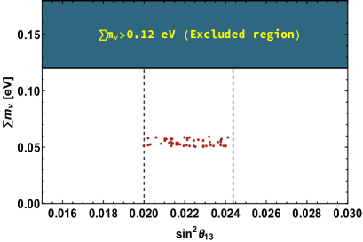
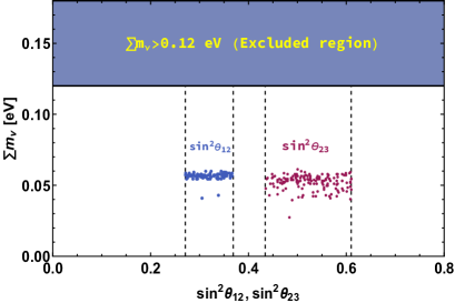
Figure 1: Left (right) panel signify the correlation of the mixing angles i.e. $\sin^{2}\theta_{13}$ ($\sin^{2}\theta_{12}$, $\sin^{2}\theta_{23}$) respectively with the sum of neutrino masses $\sum m_{i}$ (eV).

In order to make appropriate predictions of the neutrino mixing angles and other parameters within their $3\sigma$ ranges, the input parameters are generated in a random fashion. The allowed ranges of solar and atmospheric mass squared differences at $3\sigma$ level used as constraints to calculate other neutrino oscillation parameters in their $3\sigma$ ranges deSalas:2020pgw . Here, we have kept the range of modulus $\tau$ as: 0 $\lesssim\$Re$[\tau]\lesssim$ 0.5 and 0.5 $\lesssim\$Im$[\tau]\lesssim$ 2 and also the estimated range for $\mu_{0}\in[10^{-5},10]~{}\rm keV$ for obtaining the neutrino masses in normal ordering (NO). With these values, the neutrino mixing angles are then extracted using eqn. (31). The variation of the mixing angles $\sin^{2}{\theta_{13}}$ (left panel) and $\sin^{2}{\theta_{12}}$, $\sin^{2}{\theta_{23}}$ (right panel) with respect to sum of the active neutrino masses are shown in Fig. 1. Further, the variation of $\delta_{CP}$ with respect to mixing angles $\sin^{2}{\theta_{13}}$ (left panel) and $\sin^{2}{\theta_{12}}$, $\sin^{2}{\theta_{23}}$ (right panel) is shown in Fig. 2, where the vertical dashed lines represent the in $3\sigma$ ranges of the mixing angles. The left panel of Fig. 3, signifies the correlation between the observed sum of active neutrino masses ($\sum m_{i}$) and the effective neutrinoless double beta decay mass parameter ($m_{ee}$) whose maximum value is found to around 0.06 eV. In the right panel of Fig. 3, we show the correlation of Jarsklog CP invariant allowed by the neutrino data, with the reactor mixing angle, which is found to be of the order of ${\cal O}(10^{-3})$. In Fig.4 we represent the correlations between the heavy fermion masses, where, left panel is the plot expressing $M_{1}$ with $M_{2}$ and right panel is of $M_{2}$ versus $M_{3}$ in TeV scale.

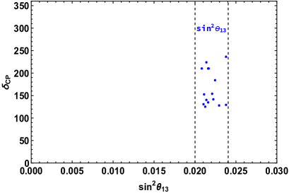
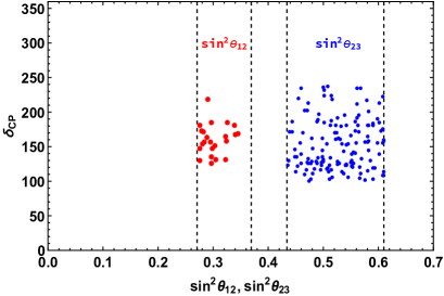
Figure 2: Left (right) panel displays the correlation between $\delta_{CP}$ w.r.t $sin^{2}\theta_{13}$ ($sin^{2}\theta_{12}$ and $sin^{2}\theta_{23}$).

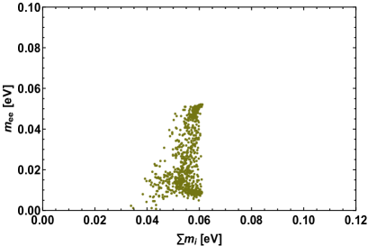
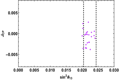
Figure 3: Left panel shows the correlation of effective neutrino mass of neutrinoless double beta decay with the sum of active neutrino masses and right panel represents a correlation between $\rm{J_{CP}}$ with respect to the reactor mixing angle.

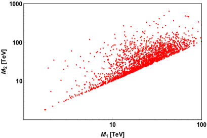
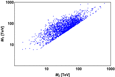
Figure 4: Left panel shows the correlation of heavy fermion masses $M_{1}$ versus $M_{2}$ and right panel represents a correlation of heavy fermion masses $M_{2}$ versus $M_{3}$ in TeV scale.

IV Comments on non-unitarity

In the section, we briefly comment on non-unitarity of neutrino mixing matrix $U^{\prime}_{\rm PMNS}$. The form for the deviation from unitarity is expressed as following Forero:2011pc

$$U^{\prime}_{\rm PMNS}\equiv\left(1-\frac{1}{2}\mathcal{F}\mathcal{F}^{\dagger}\right)U_{\rm PMNS}\;.$$ (32)

Here $\rm{U_{PMNS}}$ is the PMNS mixing matrix, used in diagonalising the mass matrix of the three light neutrinos and $\mathcal{F}$ represents the mixing of active neutrinos with the heavy fermions and its form is given by $\mathcal{F}\equiv(\mathcal{M}^{T}_{RS})^{-1}\mathcal{M}_{D}\approx({g_{D}v_{u}}/{\alpha_{RS}v_{\zeta}})$, which is hermitian in nature. The global constraints on the non-unitarity parameters Antusch:2014woa ; Blennow:2016jkn ; Fernandez-Martinez:2016lgt , come from several experimental results such as the $W$ boson mass $M_{W}$, the Weinberg angle $\theta_{W}$, several ratios of fermionic $Z$ boson as well as its invisible decay, electroweak universality, CKM unitarity bounds, and lepton flavor violations. In the context of the present model, we consider the following approximated mass values for the Dirac, Majorana mass for ${\cal S}_{L}$ and the pseudo-Dirac mass for the heavy fermions to correctly generate the observed mass square differences of the desired order as:

$$\left(\frac{m_{\nu}}{0.1~{}{\rm eV}}\right)\approx\left(\frac{\mathcal{M}_{D}}{10^{2}~{}~{}{\rm GeV}}\right)^{2}\left(\frac{{\cal M}_{\mu}}{{\rm keV}}\right)\left(\frac{\mathcal{M}_{RS}}{10^{4}~{}~{}{\rm GeV}}\right)^{-2}.$$ (33)

Using the benchmark to obtain the correct order of neutrino mass as shown in eqn.(33). Therefore, the approximated non-unitary mixing for the present model is given below:

$$|\mathcal{F}\mathcal{F}^{\dagger}|\leq\left[\begin{array}[]{ccc}1.1\times 10^{-5}&8.3\times 10^{-7}&3.8\times 10^{-6}\\ 8.3\times 10^{-7}&9.5\times 10^{-8}&5.02\times 10^{-7}\\ 3.8\times 10^{-6}&5.02\times 10^{-7}&3.05\times 10^{-7}\\ \end{array}\right]\;.$$ (37)

V comments on LFV

Lepton flavour violation is one of the most fascinating probes for new physics beyond the SM, therefore, here we investigate decay mode $\mu\to e\gamma$. Several experiments are looking for this decay mode with great effort for an improved sensitivity, and the current limit on its branching ratio is from MEG collaboration as Br$(\mu\rightarrow e\gamma)<4.2\times 10^{-13}$ TheMEG:2016wtm . There is a sizeable contribution in the present model using the $A^{\prime}_{5}$ inverse seesaw mechanism, due to the allowed light-heavy neutrino mixing. The branching ratio for the $\mu\to e\gamma$ in our model framework is given by

$${\rm Br}(\mu\to e\gamma)=\left[\frac{3}{16}\right]\left[\frac{\alpha}{2\pi}\right]\sum_{i=1}^{3}f\left(\frac{\mathcal{M}^{2}_{i}}{\mathcal{M}^{2}_{W}}\right)\left|\mathcal{F}_{\mu i}^{\ast}\,\mathcal{F}_{ei}\right|^{2}\,.$$ (38)

Here, $M_{i}$ represents the heavy fermions mass and $f(M^{2}_{i}/M^{2}_{W})$ is a loop-function Ibarra:2011xn . Also $\mathcal{F}\equiv(\mathcal{M}^{T}_{RS})^{-1}\mathcal{M}_{D}=({v_{u}}/{v_{\zeta}})(\tilde{\mathcal{M}}^{T}_{RS})^{-1}\tilde{\mathcal{M}}_{D}\approx({v_{u}}/{v_{\zeta}})$ when $\mathcal{M}_{D}$ and $\mathcal{M}_{RS}$ are of same order.

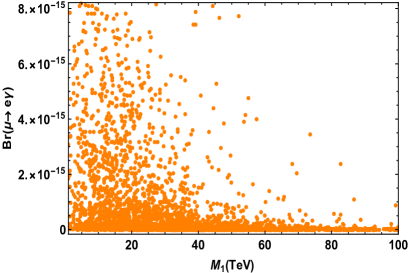
Figure 5: Plot above represents the correlation between ${\rm Br}(\mu\to e\gamma)$ with respect to (lightest heavy fermion) $M_{1}$ in TeV scale.

The branching ratio plot for the lepton flavor violating decay $\mu\to e\gamma$ is presented against lightest heavy fermion mixing mass $M_{1}$ is shown in Fig. 5. From the figure, it is evident that the predicted branching ratio is well below the current upper limit mentioned above.

VI Conclusion

We have investigated the implications of modular $A^{\prime}_{5}$ flavor symmetry on neutrino phenomenology The current model three right-handed and three left handed heavy neutral fermions to incorporate the inverse seesaw framework. The singlet scalar $\zeta$ played an imperative role in spontaneous breaking of $U(1)_{B-L}$ local symmetry and gave masses to the heavy fermions. We have considered higher order Yukawa couplings that obey the rule $k_{Y}=k_{I_{1}}+k_{I_{2}}+\cdots+k_{I_{n}}$, where $k_{Y}$ is the weight on the Yukawa coupling and $k_{I_{i}}(i=1,2,3,4\cdots)$ are the weights on the superfields under $A^{\prime}_{5}$ symmetry. This helped us to attain a specific flavor structure for neutrino mass matrix. Proceeding further, we diagonalize the mass matrix numerically and are able to vary the model parameters in such a way that they yield results compatible to $3\sigma$ limit of oscillation data. In addition, we also investigated lepton flavour violating decay mode $\mu\to e\gamma$ and found that its predicted branching ratio is well below the present experimental upper limit $4.2\times 10^{-13}$.

Appendix A The modular space of $\Gamma(5)$

In order to establish the modular forms which transform nontrivially under $\Gamma^{\prime}_{5}$, and are isomorphic to $A^{\prime}_{5}$, it is first required to find out the modular space of $\Gamma(5)$. Hence, if $k$ is an integer i.e. non-negative, the modular space ${M}_{k}\left[\Gamma(5)\right]$ bearing weight $k$ for $\Gamma(5)$ contains $5k+1$ linearly independent modular forms, which act like the basis vectors of the modular space. Thus, one can have

$${M}_{k}\left[\Gamma(5)\right]=\bigoplus_{\begin{subarray}{c}a+b=5k\\ a,b\geq 0\end{subarray}}\mathbb{C}\,\frac{\eta(5\tau)^{15k}}{\eta(\tau)^{3k}}\,{\mathfrak{k}}^{a}_{\frac{1}{5},\frac{0}{5}}(5\tau)\,{\mathfrak{k}}^{b}_{\frac{2}{5},\frac{0}{5}}(5\tau)\;,$$ (39)

below given is the Dedekind eta function $\eta(\tau)$

$$\eta(\tau)=q^{1/24}\prod_{n=1}^{\infty}\left(1-q^{n}\right)\;,$$ (40)

where, $q\equiv e^{2{\rm i}\pi\tau}$, and ${\mathfrak{k}}_{r_{1},r_{2}}(\tau)$ is the Klein form

$$\mathfrak{k}_{r_{1},r_{2}}(\tau)=q_{z}^{(r_{1}-1)/2}\left(1-q_{z}\right)\times\prod_{n=1}^{\infty}\left(1-q^{n}q_{z}\right)\left(1-q^{n}q_{z}^{-1}\right)\left(1-q^{n}\right)^{-2}\;,$$ (41)

where $(r_{1},r_{2})$ depicts a pair of rational numbers in the domain of ${\mathbb{Q}}^{2}-{\mathbb{Z}}^{2}$, $z\equiv\tau r_{1}+r_{2}$ and $q_{z}\equiv e^{2{\rm i}\pi z}$. Under the transformations of $S$ and $T$, the eta function and the Klein form change as follows

$$\begin{array}[]{cclcl}S&:{}&\eta(\tau)\rightarrow\sqrt{-{\rm i}\tau}\eta(\tau)\;,&{}\hfil&\mathfrak{k}_{r_{1},r_{2}}(\tau)\rightarrow-\dfrac{1}{\tau}\,\mathfrak{k}_{-r_{2},r_{1}}(\tau)\;,\\ T&:{}&\eta(\tau)\rightarrow e^{\rm{i}\pi/12}\eta(\tau)\;,&{}\hfil&\mathfrak{k}_{r_{1},r_{2}}(\tau)\rightarrow\mathfrak{k}_{r_{1},r_{1}+r_{2}}(\tau)\;.\end{array}$$ (44)

More information about the properties of the Kein form ${\mathfrak{k}}_{r_{1},r_{2}}(\tau)$ can be found in Refs. Ding:2019xna .

Appendix B The Kronecker product rules of $A^{\prime}_{5}$

Here we present only those product rules Wang:2020lxk which are relevant to the present model. ${\bf 3}^{\prime}\otimes{\bf 3}^{\prime}={\bf 1}_{\rm s}\oplus{\bf 3}^{\prime}_{\rm a}\oplus{\bf 5}_{\rm s}$ $\mathbf{3}\otimes\bm{3}=\mathbf{1}_{\rm s}\oplus\bm{3}_{\rm a}\oplus\bm{5}_{\rm s}$ $\left\{\begin{array}[]{l}{\bf 1}_{\rm s}:\dfrac{1}{\sqrt{3}}\left[\alpha_{1}\beta_{1}+\alpha_{2}\beta_{3}+\alpha_{3}\beta_{2}\right]\\ {\bf 3}^{\prime}_{\rm a}:\dfrac{1}{\sqrt{2}}\left[\begin{array}[]{c}\alpha_{2}\beta_{3}-\alpha_{3}\beta_{2}\\ \alpha_{1}\beta_{2}-\alpha_{2}\beta_{1}\\ \alpha_{3}\beta_{1}-\alpha_{1}\beta_{3}\end{array}\right]\\ {\bf 5}_{\rm s}:\dfrac{1}{\sqrt{6}}\left[\begin{array}[]{c}2\alpha_{1}\beta_{1}-\alpha_{2}\beta_{3}-\alpha_{3}\beta_{2}\\ \sqrt{6}\alpha_{3}\beta_{3}\\ -\sqrt{3}\left(\alpha_{1}\beta_{2}+\alpha_{2}\beta_{1}\right)\\ -\sqrt{3}\left(\alpha_{1}\beta_{3}+\alpha_{3}\beta_{1}\right)\\ \sqrt{6}\alpha_{2}\beta_{2}\end{array}\right]\end{array}\right\}.$ $\left\{\begin{array}[]{l}\mathbf{1}_{\rm s}:\dfrac{1}{\sqrt{3}}[\alpha_{1}\beta_{1}+\alpha_{2}\beta_{3}+\alpha_{3}\beta_{2}]\\ {\bf 3}_{\rm a}:\dfrac{1}{\sqrt{2}}\left[\begin{array}[]{c}\alpha_{2}\beta_{3}-\alpha_{3}\beta_{2}\\ \alpha_{1}\beta_{2}-\alpha_{2}\beta_{1}\\ \alpha_{3}\beta_{1}-\alpha_{1}\beta_{3}\end{array}\right]\\ {\bf 5}_{\rm s}:\dfrac{1}{\sqrt{6}}\left[\begin{array}[]{c}2\alpha_{1}\beta_{1}-\alpha_{2}\beta_{3}-\alpha_{3}\beta_{2}\\ -\sqrt{3}\alpha_{1}\beta_{2}-\sqrt{3}\alpha_{2}\beta_{1}\\ \sqrt{6}\alpha_{2}\beta_{2}\\ \sqrt{6}\alpha_{3}\beta_{3}\\ -\sqrt{3}\left(\alpha_{1}\beta_{3}+\alpha_{3}\beta_{1}\right)\end{array}\right]\end{array}\right\}.$

${\bf 3}\otimes{\bf 3}^{\prime}={\bf 4}\oplus{\bf 5}$

${\bf 4}\otimes{\bf 4}={\bf 1}_{\rm s}\oplus{\bf 3}_{\rm a}\oplus{\bf 3}^{\prime}_{\rm a}\oplus{\bf 4}_{\rm s}\oplus{\bf 5}_{\rm s}$

$\left\{\begin{array}[]{l}{\bf 4}:\dfrac{1}{\sqrt{3}}\left[\begin{array}[]{c}\sqrt{2}\alpha_{2}\beta_{1}+\alpha_{3}\beta_{2}\\ -\sqrt{2}\alpha_{1}\beta_{2}-\alpha_{3}\beta_{3}\\ -\sqrt{2}\alpha_{1}\beta_{3}-\alpha_{2}\beta_{2}\\ \sqrt{2}\alpha_{3}\beta_{1}+\alpha_{2}\beta_{3}\end{array}\right]\\ {\bf 5}:\dfrac{1}{\sqrt{3}}\left[\begin{array}[]{c}\sqrt{3}\alpha_{1}\beta_{1}\\ \alpha_{2}\beta_{1}-\sqrt{2}\alpha_{3}\beta_{2}\\ \alpha_{1}\beta_{2}-\sqrt{2}\alpha_{3}\beta_{3}\\ \alpha_{1}\beta_{3}-\sqrt{2}\alpha_{2}\beta_{2}\\ \alpha_{3}\beta_{1}-\sqrt{2}\alpha_{2}\beta_{3}\end{array}\right]\end{array}\right\}.$

$\left\{\begin{array}[]{l}{\bf 1}_{\rm s}:\dfrac{1}{2}\left[\alpha_{1}\beta_{4}+\alpha_{2}\beta_{3}+\alpha_{3}\beta_{2}+\alpha_{4}\beta_{1}\right]\vspace{1cm}\\ {\bf 3}_{\rm a}:\dfrac{1}{2}\left[\begin{array}[]{c}-\alpha_{1}\beta_{4}+\alpha_{2}\beta_{3}-\alpha_{3}\beta_{2}+\alpha_{4}\beta_{1}\\ \sqrt{2}\left(\alpha_{2}\beta_{4}-\alpha_{4}\beta_{2}\right)\\ \sqrt{2}\left(\alpha_{1}\beta_{3}-\alpha_{3}\beta_{1}\right)\end{array}\right]\\ {\bf 3}^{\prime}_{\rm a}:\dfrac{1}{2}\left[\begin{array}[]{c}\alpha_{1}\beta_{4}+\alpha_{2}\beta_{3}-\alpha_{3}\beta_{2}-\alpha_{4}\beta_{1}\\ \sqrt{2}\left(\alpha_{3}\beta_{4}-\alpha_{4}\beta_{3}\right)\\ \sqrt{2}\left(\alpha_{1}\beta_{2}-\alpha_{2}\beta_{1}\right)\end{array}\right]\\ {\bf 4}_{\rm s}:\dfrac{1}{\sqrt{3}}\left[\begin{array}[]{c}\alpha_{2}\beta_{4}+\alpha_{3}\beta_{3}+\alpha_{4}\beta_{2}\\ \alpha_{1}\beta_{1}+\alpha_{3}\beta_{4}+\alpha_{4}\beta_{3}\\ \alpha_{1}\beta_{2}+\alpha_{2}\beta_{1}+\alpha_{4}\beta_{4}\\ \alpha_{1}\beta_{3}+\alpha_{2}\beta_{2}+\alpha_{3}\beta_{1}\end{array}\right]\\ {\bf 5}_{\rm s}:\dfrac{1}{2\sqrt{3}}\left[\begin{array}[]{c}\sqrt{3}\left(\alpha_{1}\beta_{4}-\alpha_{2}\beta_{3}-\alpha_{3}\beta_{2}+\alpha_{4}\beta_{1}\right)\\ -\sqrt{2}\left(\alpha_{2}\beta_{4}-2\alpha_{3}\beta_{3}+\alpha_{4}\beta_{2}\right)\\ -\sqrt{2}\left(2\alpha_{1}\beta_{1}-\alpha_{3}\beta_{4}-\alpha_{4}\beta_{3}\right)\\ \sqrt{2}\left(\alpha_{1}\beta_{2}+\alpha_{2}\beta_{1}-2\alpha_{4}\beta_{4}\right)\\ -\sqrt{2}\left(\alpha_{1}\beta_{3}-2\alpha_{2}\beta_{2}+\alpha_{3}\beta_{1}\right)\end{array}\right]\end{array}\right\}.$

${\bf 5}\otimes{\bf 5}={\bf 1}_{\rm s}\oplus{\bf 3}_{\rm a}\oplus{\bf 3}^{\prime}_{\rm a}\oplus{\bf 4}_{\rm s}\oplus{\bf 4}_{\rm a}\oplus{\bf 5}_{\rm s,1}\oplus{\bf 5}_{\rm s,2}$

$\left\{\begin{array}[]{l}{\bf 1}_{\rm s}:\dfrac{1}{\sqrt{5}}\left[\alpha_{1}\beta_{1}+\alpha_{2}\beta_{5}+\alpha_{3}\beta_{4}+\alpha_{4}\beta_{3}+\alpha_{5}\beta_{2}\right]\\ {\bf 3}_{\rm a}:\dfrac{1}{\sqrt{1}0}\left[\begin{array}[]{c}\alpha_{2}\beta_{5}+2\alpha_{3}\beta_{4}-2\alpha_{4}\beta_{3}-\alpha_{5}\beta_{2}\\ -\sqrt{3}\alpha_{1}\beta_{2}+\sqrt{3}\alpha_{2}\beta_{1}+\sqrt{2}\alpha_{3}\beta_{5}-\sqrt{2}\alpha_{5}\beta_{3}\\ \sqrt{3}\alpha_{1}\beta_{5}+\sqrt{2}\alpha_{2}\beta_{4}-\sqrt{2}\alpha_{4}\beta_{2}-\sqrt{3}\alpha_{5}\beta_{1}\end{array}\right]\\ {\bf 3}^{\prime}_{\rm a}:\dfrac{1}{\sqrt{1}0}\left[\begin{array}[]{c}2\alpha_{2}\beta_{5}-\alpha_{3}\beta_{4}+\alpha_{4}\beta_{3}-2\alpha_{5}\beta_{2}\\ \sqrt{3}\alpha_{1}\beta_{3}-\sqrt{3}\alpha_{3}\beta_{1}+\sqrt{2}\alpha_{4}\beta_{5}-\sqrt{2}\alpha_{5}\beta_{4}\\ -\sqrt{3}\alpha_{1}\beta_{4}+\sqrt{2}\alpha_{2}\beta_{3}-\sqrt{2}\alpha_{3}\beta_{2}+\sqrt{3}\alpha_{4}\beta_{1}\end{array}\right]\\ {\bf 4}_{\rm s}:\dfrac{1}{\sqrt{3}0}\left[\begin{array}[]{l}\sqrt{6}\alpha_{1}\beta_{2}+\sqrt{6}\alpha_{2}\beta_{1}-\alpha_{3}\beta_{5}+4\alpha_{4}\beta_{4}-\alpha_{5}\beta_{3}\\ \sqrt{6}\alpha_{1}\beta_{3}+4\alpha_{2}\beta_{2}+\sqrt{6}\alpha_{3}\beta_{1}-\alpha_{4}\beta_{5}-\alpha_{5}\beta_{4}\\ \sqrt{6}\alpha_{1}\beta_{4}-\alpha_{2}\beta_{3}-\alpha_{3}\beta_{2}+\sqrt{6}\alpha_{4}\beta_{1}+4\alpha_{5}\beta_{5}\\ \sqrt{6}\alpha_{1}\beta_{5}-\alpha_{2}\beta_{4}+4\alpha_{3}\beta_{3}-\alpha_{4}\beta_{2}+\sqrt{6}\alpha_{5}\beta_{1}\end{array}\right]\\ {\bf 4}_{\rm a}:\dfrac{1}{\sqrt{1}0}\left[\begin{array}[]{c}\sqrt{2}\alpha_{1}\beta_{2}-\sqrt{2}\alpha_{2}\beta_{1}+\sqrt{3}\alpha_{3}\beta_{5}-\sqrt{3}\alpha_{5}\beta_{3}\\ -\sqrt{2}\alpha_{1}\beta_{3}+\sqrt{2}\alpha_{3}\beta_{1}+\sqrt{3}\alpha_{4}\beta_{5}-\sqrt{3}\alpha_{5}\beta_{4}\\ -\sqrt{2}\alpha_{1}\beta_{4}-\sqrt{3}\alpha_{2}\beta_{3}+\sqrt{3}\alpha_{3}\beta_{2}+\sqrt{2}\alpha_{4}\beta_{1}\\ \sqrt{2}\alpha_{1}\beta_{5}-\sqrt{3}\alpha_{2}\beta_{4}+\sqrt{3}\alpha_{4}\beta_{2}-\sqrt{2}\alpha_{5}\beta_{1}\end{array}\right]\\ {\bf 5}_{\rm s,1}:\dfrac{1}{\sqrt{1}4}\left[\begin{array}[]{c}2\alpha_{1}\beta_{1}+\alpha_{2}\beta_{5}-2\alpha_{3}\beta_{4}-2\alpha_{4}\beta_{3}+\alpha_{5}\beta_{2}\\ \alpha_{1}\beta_{2}+\alpha_{2}\beta_{1}+\sqrt{6}\alpha_{3}\beta_{5}+\sqrt{6}\alpha_{5}\beta_{3}\\ -2\alpha_{1}\beta_{3}+\sqrt{6}\alpha_{2}\beta_{2}-2\alpha_{3}\beta_{1}\\ -2\alpha_{1}\beta_{4}-2\alpha_{4}\beta_{1}+\sqrt{6}\alpha_{5}\beta_{5}\\ \alpha_{1}\beta_{5}+\sqrt{6}\alpha_{2}\beta_{4}+\sqrt{6}\alpha_{4}\beta_{2}+\alpha_{5}\beta_{1}\end{array}\right]\\ {\bf 5}_{\rm s,2}:\dfrac{1}{\sqrt{1}4}\left[\begin{array}[]{c}2\alpha_{1}\beta_{1}-2\alpha_{2}\beta_{5}+\alpha_{3}\beta_{4}+\alpha_{4}\beta_{3}-2\alpha_{5}\beta_{2}\\ -2\alpha_{1}\beta_{2}-2\alpha_{2}\beta_{1}+\sqrt{6}\alpha_{4}\beta_{4}\\ \alpha_{1}\beta_{3}+\alpha_{3}\beta_{1}+\sqrt{6}\alpha_{4}\beta_{5}+\sqrt{6}\alpha_{5}\beta_{4}\\ \alpha_{1}\beta_{4}+\sqrt{6}\alpha_{2}\beta_{3}+\sqrt{6}\alpha_{3}\beta_{2}+\alpha_{4}\beta_{1}\\ -2\alpha_{1}\beta_{5}+\sqrt{6}\alpha_{3}\beta_{3}-2\alpha_{5}\beta_{1}\end{array}\right]\end{array}\right\}.$

Appendix C Higher Order Yukawa couplings

All higher order Yukawa couplings are expressed in terms of the elements of $Y^{(1)}_{\widehat{\bm{6}}}$ Yukawa coupling expressed as

$$Y^{(1)}_{\widehat{\bf 6}}=\left[\begin{matrix}Y_{1}\\ Y_{2}\\ Y_{3}\\ Y_{4}\\ Y_{5}\\ Y_{6}\\ \end{matrix}\right]=\left[\begin{matrix}\widehat{e}_{1}-3\,\widehat{e}_{6}\\ 5\sqrt{2}\,\widehat{e}_{2}\\ 10\,\widehat{e}_{3}\\ 10\,\widehat{e}_{4}\\ 5\sqrt{2}\,\widehat{e}_{5}\\ -3\,\widehat{e}_{1}-\widehat{e}_{6}\\ \end{matrix}\right]\;.$$ (45)

The Yukawa couplings used in our model are expressed below and the other couplings seen in the tensor product are expressed in Wang:2020lxk

$$Y^{(2)}_{{\bf 3}} = \left[Y^{(1)}_{\widehat{\bf 6}}\otimes Y^{(1)}_{\widehat{\bf 6}}\right]_{{\bf 3}_{{\rm s},1}}=-3\left[\begin{array}[]{c}\widehat{e}^{2}_{1}-36\,\widehat{e}_{1}\widehat{e}_{6}-\widehat{e}_{6}^{2}\\ 5\sqrt{2}\,\widehat{e}_{2}(\widehat{e}_{1}-3\,\widehat{e}_{6})\\ 5\sqrt{2}\,\widehat{e}_{5}(3\,\widehat{e}_{1}+\widehat{e}_{6})\\ \end{array}\right]=-3\left[\begin{array}[]{c}Y^{2}_{1}-3Y_{1}Y_{6}-Y^{2}_{6}\\ Y_{1}Y_{2}\\ -Y_{5}Y_{6}\\ \end{array}\right],$$ (52)

$$Y^{(4)}_{\bf 3} = \left[Y^{(1)}_{\widehat{\bf 6}}\otimes Y^{(3)}_{\widehat{\bf 6},2}\right]_{{\bf 3}_{{\rm s},1}}=\frac{\sqrt{3}}{4}\left[\begin{array}[]{c}\left(Y_{1}^{2}+Y_{6}^{2}\right)\left(7Y_{1}^{2}-18Y_{1}Y_{6}-7Y_{6}^{2}\right)\\ Y_{2}\left(13Y_{1}^{3}-3Y_{1}^{2}Y_{6}-29Y_{1}Y_{6}^{2}-9Y_{6}^{3}\right)\\ -Y_{5}\left(9Y_{1}^{3}-29Y_{1}^{2}Y_{6}+3Y_{1}Y_{6}^{2}+13Y_{6}^{3}\right)\\ \end{array}\right],$$ (57)

$$Y^{(6)}_{{\bf 3},1} = \left[Y^{(1)}_{\widehat{\bf 6}}\otimes Y^{(5)}_{\widehat{\bf 2}^{\prime}}\right]_{\bf 3}=\dfrac{9\sqrt{2}}{16}\left(Y^{2}_{1}-4Y_{1}Y_{6}-Y^{2}_{6}\right)\left[\begin{array}[]{c}(Y_{1}-3Y_{6})(3Y_{1}+Y_{6})\left(3Y_{1}^{2}-2Y_{1}Y_{6}-3Y_{6}^{2}\right)\\ 2Y_{2}\left(2Y_{1}^{3}-9Y_{1}Y_{6}^{2}-3Y_{6}^{3}\right)\\ 2Y_{5}\left(3Y_{1}^{3}-9Y_{1}^{2}Y_{6}+2Y_{6}^{3}\right)\\ \end{array}\right]\;,$$ (62)

$$Y^{(6)}_{{\bf 3},2} = \left[Y^{(1)}_{\widehat{\bf 6}}\otimes Y^{(5)}_{\widehat{\bf 6},1}\right]_{{\bf 3}_{{\rm s},1}}=3\sqrt{2}\left(Y_{1}^{4}-3Y_{1}^{3}Y_{6}-Y_{1}^{2}Y_{6}^{2}+3Y_{1}Y_{6}^{3}+Y_{6}^{4}\right)\left[\begin{array}[]{c}Y_{1}^{2}-3Y_{1}Y_{6}-Y_{6}^{2}\\ Y_{1}Y_{2}\\ -Y_{5}Y_{6}\\ \end{array}\right]\;,$$ (67)

$$Y^{(6)}_{{\bf 4},1} = \left[Y^{(1)}_{\widehat{\bf 6}}\otimes Y^{(5)}_{\widehat{\bf 2}}\right]_{\bf 4}=-\dfrac{3}{4}\left(Y^{2}_{1}-4Y_{1}Y_{6}-Y^{2}_{6}\right)^{2}\left[\begin{array}[]{c}-\sqrt{2}Y_{2}(3Y_{1}+Y_{6})\\ Y_{3}(Y_{1}+Y_{6})\\ Y_{4}(Y_{1}-Y_{6})\\ \sqrt{2}Y_{5}(Y_{1}-3Y_{6})\\ \end{array}\right]\;,$$ (73)

$$Y^{(6)}_{{\bf 4},2} = \left[Y^{(1)}_{\widehat{\bf 6}}\otimes Y^{(5)}_{\widehat{\bf 2}^{\prime}}\right]_{\bf 4}=-\dfrac{\sqrt{6}}{8}\left(Y^{2}_{1}-4Y_{1}Y_{6}-Y^{2}_{6}\right)\left[\begin{array}[]{c}\sqrt{2}Y_{2}\left(Y_{1}^{3}+11Y_{1}^{2}Y_{6}+19Y_{1}Y_{6}^{2}+5Y_{6}^{3}\right)\\ Y_{3}\left(13Y_{1}^{3}-31Y_{1}^{2}Y_{6}-17Y_{1}Y_{6}^{2}-Y_{6}^{3}\right)\\ Y_{4}\left(Y_{1}^{3}-17Y_{1}^{2}Y_{6}+31Y_{1}Y_{6}^{2}+13Y_{6}^{3}\right)\\ \sqrt{2}Y_{5}\left(5Y_{1}^{3}-19Y_{1}^{2}Y_{6}+11Y_{1}Y_{6}^{2}-Y_{6}^{3}\right)\\ \end{array}\right]\;,$$ (79)

$$Y^{(6)}_{{\bf 5},1} = \left[Y^{(1)}_{\widehat{\bf 6}}\otimes Y^{(5)}_{\widehat{\bf 4}}\right]_{{\bf 5},2}=\dfrac{\sqrt{10}}{8}\left(Y^{2}_{1}-4Y_{1}Y_{6}-Y^{2}_{6}\right)\left[\begin{array}[]{c}\sqrt{3}(Y_{1}-3Y_{6})(3Y_{1}+Y_{6})\left(Y_{1}^{2}+Y_{6}^{2}\right)\\ -2Y_{2}(2Y_{1}+Y_{6})\left(2Y_{1}^{2}-3Y_{1}Y_{6}-Y_{6}^{2}\right)\\ \sqrt{2}Y_{3}\left(Y_{1}^{3}+2Y_{1}^{2}Y_{6}-11Y_{1}Y_{6}^{2}-4Y_{6}^{3}\right)\\ \sqrt{2}Y_{4}\left(4Y_{1}^{3}-11Y_{1}^{2}Y_{6}-2Y_{1}Y_{6}^{2}+Y_{6}^{3}\right)\\ 2Y_{5}(Y_{1}-2Y_{6})\left(Y_{1}^{2}-3Y_{1}Y_{6}-2Y_{6}^{2}\right)\\ \end{array}\right]\;,$$ (86)

$$Y^{(6)}_{{\bf 5},2} = \left[Y^{(1)}_{\widehat{\bf 6}}\otimes Y^{(5)}_{\widehat{\bf 6},1}\right]_{{\bf 5}_{\rm s}}=-\dfrac{1}{\sqrt{2}}\left(Y_{1}^{4}-3Y_{1}^{3}Y_{6}-Y_{1}^{2}Y_{6}^{2}+3Y_{1}Y_{6}^{3}+Y_{6}^{4}\right)\left[\begin{array}[]{c}\sqrt{2}\left(Y_{1}^{2}+Y_{6}^{2}\right)\\ 2\sqrt{6}Y_{2}(2Y_{1}+Y_{6})\\ -\sqrt{3}Y_{3}(3Y_{1}-Y_{6})\\ \sqrt{3}Y_{4}(Y_{1}+3Y_{6})\\ -2\sqrt{6}Y_{5}(Y_{1}-2Y_{6})\\ \end{array}\right]\;.$$ (93)