Cold Start Similar Artists Ranking with Gravity-Inspired Graph Autoencoders

Abstract.

On an artist’s profile page, music streaming services frequently recommend a ranked list of ”similar artists” that fans also liked. However, implementing such a feature is challenging for new artists, for which usage data on the service (e.g. streams or likes) is not yet available. In this paper, we model this cold start similar artists ranking problem as a link prediction task in a directed and attributed graph, connecting artists to their top-$k$ most similar neighbors and incorporating side musical information. Then, we leverage a graph autoencoder architecture to learn node embedding representations from this graph, and to automatically rank the top-$k$ most similar neighbors of new artists using a gravity-inspired mechanism. We empirically show the flexibility and the effectiveness of our framework, by addressing a real-world cold start similar artists ranking problem on a global music streaming service. Along with this paper, we also publicly release our source code as well as the industrial graph data from our experiments.

1. Introduction

Music streaming services heavily rely on recommender systems to help users discover and enjoy new musical content within large catalogs of millions of songs, artists and albums, with the general aim of improving their experience and engagement (Briand et al., 2021; Schedl et al., 2018; Bendada et al., 2020; Mehrotra et al., 2019). In particular, these services frequently recommend, on an artist’s profile page, a ranked list of related artists that fans also listened to or liked (Donker, 2019; Johnston, 2019; Kjus, 2016). Referred to as ”Fans Also Like” on Spotify and Soundcloud and as ”Related” or ”Similar Artists” on Amazon Music, Apple Music and Deezer, such a feature typically leverages learning to rank models (Karatzoglou et al., 2013; Schedl et al., 2018; Rafailidis and Crestani, 2017). It retrieves the most relevant artists according to similarity measures usually computed from usage data, e.g. from the proportion of shared listeners across artists (Donker, 2019; Johnston, 2019), or from more complex collaborative filtering models (Jain et al., 2020; Koren and Bell, 2015; Schedl et al., 2018) that predict similarities from the known preferences of an artist’s listeners. It has recently been described as ”one of the easiest ways” to let ”users discover new music” by Spotify (Johnston, 2019).

However, filling up such ranked lists is especially challenging for new artists. Indeed, while music streaming services might have access to some general descriptive information on these artists, listening data will however not be available upon their first release. This prevents computing the aforementioned usage-based similarity measures. As a consequence of this problem, which we refer to as cold start similar artists ranking, music streaming services usually do not propose any ”Fans Also Like” section for these artists, until (and if ever) a sufficiently large number of usage interactions, e.g. listening sessions, has been reached. Besides new artists, this usage-based approach also excludes from recommendations a potentially large part of the existing catalog with too few listening data, which raises fairness concerns (Corbett-Davies and Goel, 2018). Furthermore, while we will focus on music streaming applications, this problem encompasses the more general cold start similar items ranking issue, which is also crucial for media recommending other items such as videos (Covington et al., 2016).

In this paper, we address this problem by exploiting the fact that, as detailed in Section 3, such ”Fans Also Like” features can naturally be summarized as a directed and attributed graph, that connects each item node, e.g. each artist, to their most similar neighbors via directed links. Such a graph also incorporates additional descriptive information on nodes and links from the graph, e.g. musical information on artists. In this direction, we model cold start similar items ranking as a directed link prediction problem (Salha et al., 2019b), for new nodes gradually added into this graph.

Then, we solve this problem by leveraging recent advances in graph representation learning (Hamilton et al., 2017; Wu et al., 2021; Hamilton, 2020), and specifically directed graph autoencoders (Kipf and Welling, 2016; Salha et al., 2019b). Our proposed framework permits retrieving similar neighbors of items from node embeddings and from a gravity-inspired decoder acting as a ranking mechanism. Our work is the first transposition and analysis of gravity-inspired graph autoencoders (Salha et al., 2019b) on recommendation problems. Backed by in-depth experiments on industrial data from the global music streaming service Deezer, we show the effectiveness of our approach at addressing a real-world cold start similar artists ranking problem, outperforming several popular baselines for cold start recommendation. Last, we publicly release our code and the industrial data from our experiments. Besides making our results reproducible, we hope that such a release of real-world resources will benefit future research on this topic.

This paper is organized as follows. In Section 2, we introduce the cold start similar items ranking problem more precisely and mention previous works on related topics. In Section 3, we present our graph-based framework to address this problem. We report and discuss our experiments on Deezer data in Section 4, and we conclude in Section 5.

2. Preliminaries

2.1. Problem Formulation

Throughout this paper, we consider a catalog of $n$ recommendable items on an online service, such as music artists in our application. Each item $i$ is described by some side information summarized in an $f$-dimensional vector $x_{i}$; for artists, such a vector could for instance capture information related to their country of origin or to their music genres. These $n$ items are assumed to be ”warm”, meaning that the service considers that a sufficiently large number of interactions with users, e.g. likes or streams, has been reached for these items to ensure reliable usage data analyses.

From these usage data, the service learns an $n\times n$ similarity matrix $S$, where the element $S_{ij}\in[0,1]$ captures the similarity of item $j$ w.r.t. item $i$. Examples of some possible usage-based similarity scores $S_{ij}$ include the percentage of users interacting with item $i$ that also interacted with item $j$ (e.g. users listening to or liking both items (Johnston, 2019)), mutual information scores (Shakibian and Charkari, 2017), or more complex measures derived from collaborative filtering (Jain et al., 2020; Koren and Bell, 2015; Schedl et al., 2018). Throughout this paper, we assume that similarity scores are fixed over time, which we later discuss.

Leveraging these scores, the service proposes a similar items feature comparable to the ”Fans Also Like” described in the introduction. Specifically, along with the presentation of an item $i$ on the service, this feature recommends a ranked list of $k$ similar items to users. They correspond to the top-$k$ items $j$ such as $j\neq i$ and with highest similarity scores $S_{ij}$.

On a regular basis, ”cold” items will appear in the catalog. While the service might have access to descriptive side information on these items, no usage data will be available upon their first online release. This hinders the computation of usage-based similarity scores, thus excluding these items from recommendations until they become warm - if ever. In this paper, we study the feasibility of effectively predicting their future similar items ranked lists, from the delivery of these items i.e. without any usage data. This would enable offering such an important feature quicker and on a larger part of the catalog. More precisely, we answer the following research question: using only 1) the known similarity scores between warm items, and 2) the available descriptive information, how, and to which extent, can we predict the future ”Fans Also Like” lists that would ultimately be computed once cold items become warm?

2.2. Related Work

While collaborative filtering methods effectively learn item proximities, e.g. via the factorization of user-item interaction matrices (Van Den Oord et al., 2013; Koren and Bell, 2015), these methods usually become unsuitable for cold items without any interaction data and thus absent from these matrices (Van Den Oord et al., 2013). In such a setting, the simplest strategy for similar items ranking would consist in relying on popularity metrics (Schedl et al., 2018), e.g. to recommend the most listened artists. In the presence of descriptive information on cold items, one could also recommend items with the closest descriptions (Abbasifard et al., 2014). These heuristics are usually outperformed by hybrid models, leveraging both item descriptions and collaborative filtering on warm items (Van Den Oord et al., 2013; Hsieh et al., 2017; Wang et al., 2018; He and McAuley, 2016). They consist in:

• learning a vector space representation (an embedding) of warm items, where proximity reflects user preferences;

• then, projecting cold items into this embedding, typically by learning a model to map descriptive vectors of warm items to their embedding vectors, and then applying this mapping to cold items’ descriptive vectors.

Albeit under various formulations, this strategy has been transposed to Matrix Factorization (Van Den Oord et al., 2013; Briand et al., 2021), Collaborative Metric Learning (Hsieh et al., 2017; Lee et al., 2018) and Bayesian Personalized Ranking (He and McAuley, 2016; Barkan et al., 2019); in practice, a deep neural network often acts as the mapping model. The retrieved similar items are then the closest ones in the embedding. Other deep learning approaches were also recently proposed for item cold start, with promising performances. DropoutNet (Volkovs et al., 2017) processes both usage and descriptive data, and is explicitly trained for cold start through a dropout (Srivastava et al., 2014) simulation mechanism. MeLU (Lee et al., 2019) deploys a meta-learning paradigm to learn embeddings in the absence of usage data. CVAE (Li and She, 2017) leverages a Bayesian generative process to sample cold embedding vectors, via a collaborative variational autoencoder.

While they constitute relevant baselines, these models do not rely on graphs, contrary to our work. Graph-based recommendation has recently grown at a fast pace (see the surveys of (Wang et al., 2021; Wu et al., 2020)), including in industrial applications (Wang et al., 2018; Ying et al., 2018). Existing research widely focuses on bipartite user-item graphs (Wang et al., 2021). Notably, STAR-GCN (Zhang et al., 2019) addresses cold start by reconstructing user-item links using stacked graph convolutional networks, extending ideas from (Berg et al., 2018; Kipf and Welling, 2016). Instead, recent efforts (Qian et al., 2019, 2020) emphasized the relevance of leveraging - as we will - graphs connecting items together, along with their attributes. In this direction, the work closest to ours might be the recent DEAL (Hao et al., 2020) who, thanks to an alignment mechanism, predicts links in such graphs for new nodes having only descriptive information. We will also compare to DEAL; we nonetheless point out that their work focused on undirected graphs, and did not consider ranking settings.

3. A Graph-Based Framework for Cold Start Similar Items Ranking

In this section, we present our proposed graph-based framework to address the cold start similar items ranking problem.

3.1. Similar Items Ranking as a Directed Link Prediction Task

We argue that ”Fans Also Like” features can naturally be summarized as a graph structure with $n$ nodes and $n\times k$ edges. Nodes are warm recommendable items from the catalog, e.g. music artists with enough usage data according to the service’s internal rules. Each item node points to its $k$ most similar neighbors via a link, i.e. an edge. This graph is:

• directed: edges have a direction, leading to asymmetric relationships. For instance, while most fans of a little known reggae band might listen to Bob Marley (Marley thus appearing among their similar artists), Bob Marley’s fans will rarely listen to this band, which is unlikely to appear back among Bob Marley’s own similar artists.

• weighted: among the $k$ neighbors of node $i$, some items are more similar to $i$ than others (hence the ranking). We capture this aspect by equipping each directed edge $(i,j)$ from the graph with a weight corresponding to the similarity score $S_{ij}$. More formally, we summarize our graph structure by the $n\times n$ adjacency matrix $A$, where the element $A_{ij}=S_{ij}$ if $j$ is one of the $k$ most similar items w.r.t. $i$, and where $A_{ij}=0$ otherwise.

• attributed: as explained in Section 2.1, each item $i$ is also described by a vector $x_{i}\in\mathbb{R}^{f}$. In the following, we denote by $X$ the $n\times f$ matrix stacking up all descriptive vectors from the graph, i.e. the $i$-th row of $X$ is $x_{i}$.

Then, we model the release of a cold recommendable item in the catalog as the addition of a new node in the graph, together with its side descriptive vector. As usage data and similarity scores are unavailable for this item, it is observed as isolated, i.e. it does not point to $k$ other nodes. In our framework, we assume that these $k$ missing directed edges - and their weights - are actually masked. They point to the $k$ nodes with highest similarity scores, as would be identified by the service once it collects enough usage data to consider the item as warm, according to the service’s criteria. These links and their scores, ultimately revealed, are treated as ground-truth in the remainder of this work.

From this perspective, the cold start similar items ranking problem consists in a directed link prediction task (Schall, 2014; Salha et al., 2019b; Lu and Zhou, 2011). Specifically, we aim at predicting the locations and weights - i.e. estimated similarity scores - of these $k$ missing directed edges, and at comparing predictions with the actual ground-truth edges ultimately revealed, both in terms of:

• prediction accuracy: do we retrieve the correct locations of missing edges in the graph?

• ranking quality: are the retrieved edges correctly ordered, in terms of similarity scores?

3.2. From Similar Items Graphs to Directed Node Embeddings

Locating missing links in graphs has been the objective of significant research efforts from various fields (Schall, 2014; Salha et al., 2019b; Lu and Zhou, 2011; Liben-Nowell and Kleinberg, 2007). While this problem has been historically addressed via the construction of hand-engineered node similarity metrics, such as the popular Adamic-Adar, Jaccard or Katz measures (Liben-Nowell and Kleinberg, 2007), significant improvements were recently achieved by methods directly learning node representations summarizing the graph structure (Hamilton et al., 2017; Wu et al., 2021; Kipf and Welling, 2017, 2016; Hamilton, 2020). These methods represent each node $i$ as a vector $z_{i}\in\mathbb{R}^{d}$ (with $d\ll n$) in a node embedding space where structural proximity should be preserved, and learned by using matrix factorization (Cao et al., 2015), random walks (Perozzi et al., 2014), or graph neural networks (Kipf and Welling, 2017; Wu et al., 2021). Then, they estimate the probability of a missing edge between two nodes by evaluating their proximity in this embedding (Kipf and Welling, 2016; Hamilton et al., 2017).

In this paper, we build upon these advances and thus learn node embeddings to tackle link prediction in our similar items graph. Specifically, we propose to leverage gravity-inspired graph (variational) autoencoders, recently introduced in a previous work from Deezer (Salha et al., 2019b). As detailed in Section 3.3, these models are doubly advantageous for our application:

• Foremost, they can effectively process node attribute vectors in addition to the graph, contrary to some popular alternatives such as DeepWalk (Perozzi et al., 2014) and standard Laplacian eigenmaps (Belkin and Niyogi, 2001). This will help us add some cold nodes, isolated but equipped with some descriptions, into an existing warm node embedding.

• Simultaneously, they were specifically designed to address directed link prediction from embeddings, contrary to the aforementioned alternatives or to standard graph autoencoders (Kipf and Welling, 2016).

In the following, we first recall key concepts related to gravity-inspired graph (variational) autoencoders, in Section 3.3. Then, we transpose them to similar items ranking, in Section 3.4. To the best of our knowledge, our work constitutes the first analysis of these models on a recommendation problem and, more broadly, on an industrial application.

3.3. Gravity-Inspired Graph (Variational) Autoencoders

3.3.1. Overview

To predict the probability of a missing edge - and its weight - between two nodes $i$ and $j$ from some embedding vectors $z_{i}$ and $z_{j}$, most existing methods rely on symmetric measures, such as the Euclidean distance between these vectors $||z_{i}-z_{j}||_{2}$ (Hamilton et al., 2017) or their inner-product $z^{T}_{i}z_{j}$ (Kipf and Welling, 2016). However, due to this symmetry, predictions will be identical for both edge directions $i\rightarrow j$ and $j\rightarrow i$. This is undesirable for directed graphs, where $A_{ij}\neq A_{ji}$ in general.

Salha et al. (Salha et al., 2019b) addressed this problem by equipping $z_{i}$ vectors with masses, and then taking inspiration from Newton’s second law of motion (Newton, 1687). Considering two objects $1$ and $2$ with positive masses $m_{1}$ and $m_{2}$, and separated by a distance $r>0$, the physical acceleration $a_{1\rightarrow 2}$ (resp. $a_{2\rightarrow 1}$) of $1$ towards $2$ (resp. $2$ towards $1$) due to gravity (Salha et al., 2019b) is $a_{1\rightarrow 2}=\frac{Gm_{2}}{r^{2}}$ (resp. $a_{2\rightarrow 1}=\frac{Gm_{1}}{r^{2}}$), where $G$ denotes the gravitational constant (Cavendish, 1798). One observes that $a_{1\rightarrow 2}>a_{2\rightarrow 1}$ when $m_{2}>m_{1}$, i.e. that the acceleration of the less massive object towards the more massive one is higher. Transposing these notions to node embedding vectors $z_{i}$ augmented with masses $m_{i}$ for each node $i$, Salha et al. (Salha et al., 2019b) reconstruct asymmetric links by using $a_{i\rightarrow j}$ (resp. $a_{j\rightarrow i}$) as an indicator of the likelihood that node $i$ is connected to $j$ (resp. $j$ to $i$) via a directed edge, setting $r=\|z_{i}-z_{j}\|_{2}$. Precisely, they use the logarithm of $a_{i\rightarrow j}$, limiting accelerations towards very central nodes (Salha et al., 2019b), and add a sigmoid activation $\sigma(x)=1/(1+e^{-x})\in]0,1[$. Therefore, for weighted graphs, the output is an estimation $\hat{A}_{ij}$ of some true weight $A_{ij}\in[0,1]$. For unweighted graphs, it corresponds to the probability of a missing edge:

(1) $$\hat{A}_{ij}=\sigma(\log a_{i\rightarrow j})=\sigma(\log\frac{Gm_{j}}{\|z_{i}-z_{j}\|_{2}^{2}})=\sigma(\underbrace{\log Gm_{j}}_{\text{denoted }\tilde{m}_{j}}-\log\|z_{i}-z_{j}\|_{2}^{2}).$$

3.3.2. Gravity-Inspired Graph AE

To learn such masses and embedding vectors from an $n\times n$ adjacency matrix $A$, potentially completed with an $n\times f$ node attributes matrix $X$, Salha et al. (Salha et al., 2019b) introduced gravity-inspired graph autoencoders. They build upon the graph extensions of autoencoders (AE) (Kipf and Welling, 2016; Tian et al., 2014; Wang et al., 2016), that recently appeared among the state-of-the-art approaches for (undirected) link prediction in numerous applications (Salha et al., 2021; Salha et al., 2020; Wang et al., 2016; Kipf and Welling, 2016; Grover et al., 2019; Hasanzadeh et al., 2019). Graph AE are a family of models aiming at encoding nodes into an embedding space from which decoding i.e. reconstructing the graph should ideally be possible, as, intuitively, this would indicate that such representations preserve important characteristics from the initial graph.

In the case of gravity-inspired graph AE, the encoder is a graph neural network (GNN) (Hamilton et al., 2017) processing $A$ and $X$ (we discuss architecture choices in Section 3.4.1), and returning an $n\times(d+1)$ matrix $\tilde{Z}$. The $i$-th row of $\tilde{Z}$ is a $(d+1)$-dimensional vector $\tilde{z}_{i}$. The $d$ first dimensions of $\tilde{z}_{i}$ correspond to the embedding vector $z_{i}$ of node $i$; the last dimension corresponds to the mass $\tilde{m}_{i}$. Then, a decoder reconstructs $\hat{A}$ from the aforementioned acceleration formula:

(2) $$\tilde{Z}=\text{GNN}(A,X),\text{ then }\forall(i,j)\in\{1,...,n\}^{2},\hat{A}_{ij}=\sigma(\tilde{m}_{j}-\log\|z_{i}-z_{j}\|_{2}^{2}).$$

During training, the GNN’s weights are tuned by minimizing a reconstruction loss capturing the quality of the reconstruction $\hat{A}$ w.r.t. the true $A$, using gradient descent (Goodfellow et al., 2016). In (Salha et al., 2019b), this loss is formulated as a standard weighted cross entropy  (Salha et al., 2020).

3.3.3. Gravity-Inspired Graph VAE

Introduced as a probabilistic variant of gravity-inspired graph AE, gravity-inspired graph variational autoencoders (VAE) (Salha et al., 2019b) extend the graph VAE model from Kipf and Welling (Kipf and Welling, 2016), originally designed for undirected graphs. They provide an alternative strategy to learn $\tilde{Z}$, assuming that $\tilde{z}_{i}$ vectors are drawn from Gaussian distributions - one for each node - that must be learned. Formally, they consider the following inference model  (Salha et al., 2019b), acting as an encoder: $q(\tilde{Z}|A,X)=\prod_{i=1}^{n}q(\tilde{z}_{i}|A,X)$, with $q(\tilde{z}_{i}|A,X)=\mathcal{N}(\tilde{z}_{i}|\mu_{i},\text{diag}(\sigma_{i}^{2}))$.

Gaussian parameters are learned from two GNNs, i.e. $\mu=\text{GNN}_{\mu}(A,X)$, with $\mu$ denoting the $n\times(d+1)$ matrix stacking up mean vectors $\mu_{i}$. Similarly, $\log\sigma=\text{GNN}_{\sigma}(A,X)$. Finally, a generative model decodes $A$ using, as above, the acceleration formula: $p(A|\tilde{Z})=\prod_{i=1}^{n}\prod_{j=1}^{n}p(A_{ij}|\tilde{z}_{i},\tilde{z}_{j})$, with $\textbf{}p(A_{ij}|\tilde{z}_{i},\tilde{z}_{j})=\hat{A}_{ij}=\sigma(\tilde{m}_{j}-\log\|z_{i}-z_{j}\|_{2}^{2})$.

During training, weights from the two GNN encoders are tuned by maximizing, as a reconstruction quality measure, a tractable variational lower bound (ELBO) of the model’s likelihood (Kipf and Welling, 2016; Salha et al., 2019b), using gradient descent. We refer to (Salha et al., 2019b) for the exact formula of this ELBO loss, and to (Kingma and Welling, 2014; Doersch, 2016) for details on derivations of variational bounds for VAE models.

Besides constituting generative models with powerful applications to various graph generation problems (Liu et al., 2018; Ma et al., 2018), graph VAE models emerged as competitive alternatives to graph AE on some link prediction problems (Salha et al., 2019b; Salha et al., 2020; Hasanzadeh et al., 2019; Kipf and Welling, 2016). We therefore saw value in considering both gravity-inspired graph AE and gravity-inspired graph VAE in our work.

3.4. Cold Start Similar Items Ranking using Gravity-Inspired Graph AE/VAE

In this subsection, we now explain how we build upon these models to address cold start similar items ranking.

3.4.1. Encoding Cold Nodes with GCNs

In this paper, our GNN encoders will be graph convolutional networks (GCN) (Kipf and Welling, 2017). In a GCN with $L$ layers, with input layer $H^{(0)}=X$ corresponding to node attributes, and output layer $H^{(L)}$ (with $H^{(L)}=\tilde{Z}$ for AE, and $H^{(L)}=\mu$ or $\log\sigma$ for VAE), we have $H^{(l)}=\text{ReLU}(\tilde{A}H^{(l-1)}W^{(l-1)})$ for $l\in\{1,...,L-1\}$ and $H^{(L)}=\tilde{A}H^{(L-1)}W^{(L-1)}$. Here, $\tilde{A}$ denotes the out-degree normalized version of $A$ (Salha et al., 2019b). Therefore, at each layer, each node averages the representations from its neighbors (and itself), with a ReLU activation: $\text{ReLU}(x)=\max(x,0)$. $W^{(0)},...,W^{(L-1)}$ are the weight matrices to tune. More precisely, we will implement 2-layer GCNs, meaning that, for AE:

(3) $$\tilde{Z}=\tilde{A}\text{ReLU}(\tilde{A}XW^{(0)})W^{(1)}.$$

For VAE, $\mu=\tilde{A}\text{ReLU}(\tilde{A}XW^{(0)}_{\mu})W^{(1)}_{\mu}$, $\log\sigma=\tilde{A}\text{ReLU}(\tilde{A}XW^{(0)}_{\sigma})W^{(1)}_{\sigma}$, and $\tilde{Z}$ is then sampled from $\mu$ and $\log\sigma$. As all outputs are $n\times(d+1)$ matrices and $X$ is an $n\times f$ matrix, then $W^{(0)}$ (or, $W^{(0)}_{\mu}$ and $W^{(0)}_{\sigma}$) is an $f\times d_{\text{hidden}}$ matrix, with $d_{\text{hidden}}$ the hidden layer dimension, and $W^{(1)}$ (or, $W^{(1)}_{\mu}$ and $W^{(1)}_{\sigma}$) is an $d_{\text{hidden}}\times(d+1)$ matrix.

We rely on GCN encoders as they permit incorporating new nodes, attributed but isolated in the graph, into an existing embedding. Indeed, let us consider an autoencoder trained from some $A$ and $X$, leading to optimized weights $W^{(0)}$ and $W^{(1)}$ for some GCN. If $m\geq 1$ cold nodes appear, along with their $f$-dimensional description vectors:

• $A$ becomes $A^{\prime}$, an $(n+m)\times(n+m)$ adjacency matrix, with $m$ new rows and columns filled with zeros.

• $X$ becomes $X^{\prime}$, an $(n+m)\times f$ attribute matrix, concatenating $X$ and the $f$-dim descriptions of the $m$ new nodes.

• We derive embedding vectors and masses of new nodes through a forward pass into the GCN previously trained on warm nodes, i.e. by computing the $(n+m)\times(d+1)$ new embedding matrix $\tilde{Z}^{\prime}=\tilde{A}^{\prime}\text{ReLU}(\tilde{A}^{\prime}X^{\prime}W^{(0)})W^{(1)}$.

We emphasize that the choice of GCN encoders is made without loss of generality. Our framework remains valid for any encoder similarly processing new attributed nodes. In our experiments, 2-layer GCNs reached better or comparable results w.r.t. some considered alternatives, namely deeper GCNs, linear encoders (Salha et al., 2020), and graph attention networks (Veličković et al., 2018).

3.4.2. Ranking Similar Items

After projecting cold nodes into the warm embedding, we use the gravity-inspired decoder to predict their masked connections. More precisely, in our experiments, we add a hyperparameter $\lambda\in\mathbb{R}^{+}$ to equation (1) for flexibility. The estimated similarity weight $\hat{A}_{ij}$ between some cold node $i$ and another node $j$ is thus:

(4) $$\hat{A}_{ij}=\sigma(\underbrace{\tilde{m}_{j}}_{\text{influence of $j$}}-\lambda\times\underbrace{\log\|z_{i}-z_{j}\|_{2}^{2}}_{\text{proximity of $i$ and $j$}}).$$

Then, the predicted top-$k$ most similar items of $i$ will correspond to the $k$ nodes $j$ with highest estimated weights $\hat{A}_{ij}$.

We interpret equation (4) in terms of influence/proximity trade-off. The influence part of (4) indicates that, if two nodes $j$ and $l$ are equally close to $i$ in the embedding (i.e. $\|z_{i}-z_{j}\|_{2}=\|z_{i}-z_{l}\|_{2}$), then $i$ will more likely points towards the node with the largest mass (i.e. ”influence”; we will compare these masses to popularity metrics in experiments). The proximity part of (4) indicates that, if $j$ and $l$ have the same mass (i.e. $\tilde{m}_{j}=\tilde{m}_{l}$), then $i$ will more likely points towards its closest neighbor, which could e.g. capture a closer musical similarity for artists. As illustrated in Section 4.3.4, tuning $\lambda$ will help us flexibly balance between these two aspects, and thus control for popularity biases (Schedl et al., 2018) in our recommendations.

3.4.3. On Complexity

Training models via full-batch gradient descent requires reconstructing the entire $\hat{A}$, which has an $O(dn^{2})$ time complexity due to the evaluation of pairwise distances (Salha et al., 2019a, b). While we will follow this strategy, our released code will also implement FastGAE (Salha et al., 2021), a fast optimization method which approximates losses by decoding random subgraphs of $O(n)$ size. Moreover, projecting cold nodes in an embedding only requires a single forward GCN pass, with linear time complexity w.r.t. the number of edges (Kipf and Welling, 2017; Salha et al., 2020). This is another advantage of using GCNs w.r.t. more complex encoders. Last, retrieving the top-$k$ accelerations boils down to a nearest neighbors search in a $O(ndk)$ time, which could even be improved in future works with approximate search methods (Abbasifard et al., 2014).

4. Experimental Evaluation

We now present the experimental evaluation of our framework on music artists data from the Deezer production system.

4.1. Experimental Setting: Ranking Similar Artists on a Music Streaming Service

4.1.1. Dataset

We consider a directed graph of 24 270 artists with various musical characteristics (see below), extracted from the music streaming service Deezer. Each artist points towards $k=20$ other artists. They correspond, up to internal business rules, to the top-20 artists from the same graph that would be recommended by our production system on top of the ”Fans Also Like/Similar Artists” feature illustrated in Figure 1. Each directed edge $(i,j)$ has a weight $A_{ij}$ normalized in the $[0,1]$ set; for unconnected pairs, $A_{ij}=0$. It corresponds to the similarity score of artist $j$ w.r.t. $i$, computed on a weekly basis from usage data of millions of Deezer users. More precisely, weights are based on mutual information scores (Shakibian and Charkari, 2017) from artist co-occurrences among streams. Roughly, they compare the probability that a user listens to the two artists, to their global listening frequencies on the service, and they are normalized at the artist level through internal heuristics and business rules (some details on exact score computations are voluntarily omitted for confidentiality reasons). In the graph, edges correspond to the 20 highest scores for each node. In general, $A_{ij}\neq A_{ji}$. In particular, $j$ might be the most similar artist of $i$ while $i$ does not appear among the top-20 of $j$.

We also have access to descriptions of these artists, either extracted through the musical content or provided by record labels. Here, each artist $i$ will be described by an attribute vector $x_{i}$ of dimension $f=56$, concatenating:

• A 32-dimensional genre vector. Deezer artists are described by music genres (Epure et al., 2020), among more than 300. 32-dim embeddings are learned from these genres, by factorizing a co-occurrence matrix based on listening usages with SVD (Koren et al., 2009). Then, the genre vector of an artist is the average of embedding vectors of his/her music genres.

• A 20-dimensional country vector. It corresponds to a one-hot encoding vector, indicating the country of origin of an artist, among the 19 most common countries on Deezer, and with a 20^th category gathering all other countries.

• A 4-dimensional mood vector. It indicates the average and standard deviations of the valence and arousal scores across an artist’s discography. In a nutshell, valence captures whether each song has a positive or negative mood, while arousal captures whether each song has a calm or energetic mood (Russell, 1980; Delbouys et al., 2018; Huang et al., 2016). These scores are computed internally, from audio data and using a deep neural network inspired from the work of Delbouys et al. (Delbouys et al., 2018).

While some of these features are quite general, we emphasize that the actual Deezer app also gathers more refined information on artists, e.g. from audio or textual descriptions. They are undisclosed and unused in these experiments.

Figure 1. Similar artists recommended on the website version of Deezer. The mobile app proposes identical recommendations.

4.1.2. Problem

We consider the following similar artists ranking problem. Artists are split into a training set, a validation set and a test set gathering 80%, 10% and 10% of artists respectively. The training set corresponds to warm artists. Artists from the validation and test sets are the cold nodes: their edges are masked, and they are therefore observed as isolated in the graph. Their 56-dimensional descriptions are available. We evaluate the ability of our models at retrieving these edges, with correct weight ordering. As a measure of prediction accuracy, we will report Recall@K scores. They indicate, for various $K$, which proportion of the 20 ground-truth similar artists appear among the top-$K$ artists with largest estimated weights. Moreover, as a measure of ranking quality, we will also report the widely used Mean Average Precision at $K$ (MAP@K) and Normalized Discounted Cumulative Gain  at $K$ (NDCG@K) scores.

4.1.3. Dataset and Code Release

We publicly release our industrial data (i.e. the complete graph, all weights and all descriptive vectors) as well as our source code on GitHub. Besides making our results fully reproducible, such a release publicly provides a new benchmark dataset to the research community, permitting the evaluation of comparable graph-based recommender systems on real-world resources.

4.2. List of Models and Baselines

We now describe all methods considered in our experiments. All embeddings have $d=32$, which we will discuss. Also, all hyperparameters mentioned thereafter were tuned by optimizing NDCG@20 scores on the validation set.

4.2.1. Gravity-Inspired Graph AE/VAE

We follow our framework from Section 3.4 to embed cold nodes. For both AE and VAE, we use 2-layer GCN encoders with 64-dim hidden layer, and 33-dim output layer (i.e. 32-dim $z_{i}$ vectors, plus the mass), trained for 300 epochs. We use Adam optimizer (Kingma and Ba, 2015), with a learning rate of 0.05, without dropout, performing full-batch gradient descent, and using the reparameterization trick (Kingma and Welling, 2014) for VAE. We set $\lambda$ = 5 in the decoder of (4) and discuss the impact of $\lambda$ thereafter. Our adaptation of these models builds upon the Tensorflow code of Salha et  al.  (Salha et al., 2019b).

4.2.2. Other Methods based on the Directed Artist Graph

We compare gravity-inspired graph AE/VAE to standard graph AE /VAE models (Kipf and Welling, 2017), with a similar setting as above. These models use symmetric inner-product decoders i.e. $\hat{A}_{ij}=\sigma(z^{T}_{i}z_{j})$, therefore ignoring directionalities. Moreover, we implement source-target graph AE/VAE, used as a baseline in (Salha et al., 2019b). They are similar to standard graph AE/VAE, except that they decompose the 32-dim vectors $z_{i}$ into a source vector $z^{(s)}_{i}=z_{i[1:16]}$ and a target vector $z^{(t)}_{i}=z_{i[17:32]}$, and then decode edges as follows: $\hat{A}_{ij}=\sigma(z^{(s)T}_{i}z^{(t)}_{j})$ and $\hat{A}_{ji}=\sigma(z^{(s)T}_{j}z^{(t)}_{i})$ ($\neq\hat{A}_{ij}$ in general). They reconstruct directed links, as gravity models, and are therefore relevant baselines for our evaluation. Last, we also test the recent DEAL model (Hao et al., 2020) mentioned in Section 2.2, and designed for inductive link prediction on new isolated but attributed nodes. We used the authors’ PyTorch implementation, with similar attribute and structure encoders, alignment mechanism, loss and cosine predictions as their original model (Hao et al., 2020).

4.2.3. Other Baselines

In addition, we compare our proposed framework to four popularity-based baselines:

• Popularity: recommends the $K$ most popular artists on Deezer (with $K$ as in Section 4.1.2).

• Popularity by country: recommends the $K$ most popular artists from the country of origin of the cold artist.

• In-degree: recommends the $K$ artists with highest in-degrees in the graph, i.e. sum of weights pointing to them.

• In-degree by country: proceeds as In-degree, but on warm artists from the country of origin of the cold artist.

We also consider three baselines only or mainly based on musical descriptions $x_{i}$ and not on usage data:

• $K$-NN: recommends the $K$ artists with closest $x_{i}$ vectors, from a nearest neighbors search with Euclidean distance.

• $K$-NN + Popularity and $K$-NN + In-degree: retrieve the 200 artists with closest $x_{i}$ vectors, then recommends the $K$ most popular ones among these 200 artists, ranked according to popularity and in-degree values respectively.

We also implement SVD+DNN, which follows the ”embedding+mapping” strategy from Section 2.2 by 1) computing an SVD (Koren et al., 2009) of the warm artists similarity matrix, learning 32-dim $z_{i}$ vectors, 2) training a 3-layer neural network (with layers of dimension 64, 32 and 32, trained with Adam (Kingma and Ba, 2015) and a learning rate of 0.01) to map warm $x_{i}$ vectors to $z_{i}$ vectors, and 3) projecting cold artists into the SVD embedding through this mapping. Last, among deep learning approaches from Section 2.2 (CVAE, DropoutNet, MeLU, STAR-GCN), we report results from the two best methods on our dataset, namely DropoutNet (Volkovs et al., 2017) and STAR-GCN (Zhang et al., 2019), using the authors’ implementations with careful fine-tuning on validation artists. Similar artists ranking is done via a nearest neighbors search in the resulting embedding spaces.

4.3. Results

Table 1. Cold start similar artists ranking: performances on test set.

Methods	Recall@K (in %)			MAP@K (in %)			NDCG@K (in %)
($d=32$)	$K=20$	$K=100$	$K=200$	$K=20$	$K=100$	$K=200$	$K=20$	$K=100$	$K=200$
Popularity	0.02	0.44	1.38	¡0.01	0.03	0.12	0.01	0.17	0.44
Popularity by country	2.76	12.38	18.98	0.80	3.58	6.14	2.14	6.41	8.76
In-degree	0.91	3.43	6.85	0.15	0.39	0.86	0.67	1.69	2.80
In-degree by country	5.46	16.82	23.52	2.09	5.43	7.73	5.00	10.19	12.64
$K$-NN on $x_{i}$	4.41	13.54	19.80	1.14	3.38	5.39	4.29	8.83	11.22
$K$-NN + Popularity	5.73	15.87	19.83	1.66	4.32	5.74	4.86	10.03	11.76
$K$-NN + In-degree	7.49	17.29	18.76	2.78	5.60	6.18	7.41	12.48	13.14
SVD + DNN	6.42 $\pm$ 0.96	21.83 $\pm$ 1.21	35.01 $\pm$ 1.41	2.25 $\pm$ 0.67	6.36 $\pm$ 1.19	11.52 $\pm$ 1.98	6.05 $\pm$ 0.75	12.91 $\pm$ 0.92	17.89 $\pm$ 0.95
STAR-GCN	10.03 $\pm$ 0.56	31.45 $\pm$ 1.09	43.92 $\pm$ 1.10	3.10 $\pm$ 0.32	10.64 $\pm$ 0.54	16.62 $\pm$ 0.68	10.07 $\pm$ 0.40	21.17 $\pm$ 0.69	25.99 $\pm$ 0.75
DropoutNet	12.96 $\pm$ 0.54	37.59 $\pm$ 0.76	49.93 $\pm$ 0.82	4.18 $\pm$ 0.30	13.61 $\pm$ 0.55	20.12 $\pm$ 0.67	13.12 $\pm$ 0.68	25.61 $\pm$ 0.72	30.52 $\pm$ 0.78
DEAL	12.80 $\pm$ 0.52	37.98 $\pm$ 0.59	50.75 $\pm$ 0.72	4.15 $\pm$ 0.25	14.01 $\pm$ 0.44	20.92 $\pm$ 0.54	12.78 $\pm$ 0.53	25.70 $\pm$ 0.62	30.69 $\pm$ 0.70
Graph AE	7.30 $\pm$ 0.51	25.92 $\pm$ 0.95	40.37 $\pm$ 1.11	2.81 $\pm$ 0.29	7.97 $\pm$ 0.47	14.24 $\pm$ 0.67	6.32 $\pm$ 0.39	15.54 $\pm$ 0.66	20.94 $\pm$ 0.72
Graph VAE	10.01 $\pm$ 0.52	34.00 $\pm$ 1.06	49.72 $\pm$ 1.14	3.53 $\pm$ 0.27	11.68 $\pm$ 0.52	19.46 $\pm$ 0.70	10.09 $\pm$ 0.58	21.37 $\pm$ 0.73	27.31 $\pm$ 0.75
Sour.-Targ. Graph AE	12.21 $\pm$ 1.30	39.52 $\pm$ 3.53	56.25 $\pm$ 3.57	4.62 $\pm$ 0.81	14.67 $\pm$ 2.33	23.60 $\pm$ 2.85	12.42 $\pm$ 1.39	25.45 $\pm$ 3.37	31.80 $\pm$ 3.38
Sour.-Targ. Graph VAE	13.52 $\pm$ 0.64	42.68 $\pm$ 0.69	59.51 $\pm$ 0.76	5.19 $\pm$ 0.31	16.07 $\pm$ 0.40	25.48 $\pm$ 0.55	13.60 $\pm$ 0.73	27.81 $\pm$ 0.56	34.19 $\pm$ 0.59
Gravity Graph AE	18.33 $\pm$ 0.45	52.26 $\pm$ 0.90	67.85 $\pm$ 0.98	6.64 $\pm$ 0.25	21.19 $\pm$ 0.55	30.67 $\pm$ 0.68	18.64 $\pm$ 0.47	35.77 $\pm$ 0.66	41.42 $\pm$ 0.68
Gravity Graph VAE	16.59 $\pm$ 0.50	49.51 $\pm$ 0.78	65.70 $\pm$ 0.75	5.66 $\pm$ 0.35	19.07 $\pm$ 0.57	28.66 $\pm$ 0.59	16.74 $\pm$ 0.55	33.34 $\pm$ 0.66	39.29 $\pm$ 0.64

4.3.1. Performances

Table 1 reports mean performance scores for all models, along with standard deviations over 20 runs for models with randomness due to weights initialization in GCNs or neural networks. Popularity and In-degree appear as the worst baselines. Their scores significantly improve by focusing on the country of origin of cold artists (e.g. with a Recall@100 of 12.38% for Popularity by country, v.s. 0.44% for Popularity). Besides, we observe that methods based on a direct $K$-NN search from $x_{i}$ attributes are outperformed by the more elaborated cold start methods leveraging both attributes and warm usage data. In particular, DropoutNet, as well as the graph-based DEAL, reach stronger results than SVD+DNN and STAR-GCN. They also surpass standard graph AE and VAE (e.g. with a +6.46 gain in average NDCG@20 score for DEAL w.r.t. graph AE), but not the AE/VAE extensions that explicitly model edges directionalities, i.e. source-target graph AE/VAE and, even more, gravity-inspired graph AE/VAE, that provide the best recommendations. It emphasizes the effectiveness of our framework, both in terms of prediction accuracy (e.g. with a top 67.85% average Recall@200 for gravity-inspired graph AE) and of ranking quality (e.g. with a top 41.42% average NDCG@200 for this same method). Moreover, while embeddings from Table 1 have $d=32$, we point out that gravity-inspired models remained superior on our tests with $d=64$ and $d=128$. Also, VAE methods tend to outperform their deterministic counterparts for standard and source-target models, while the contrary conclusion emerges on gravity-inspired models. This confirms the value of considering both settings when testing these models on novel applications.

4.3.2. On the mass parameter

In Figure 3, we visualize some artists and their estimated masses. At first glance, one might wonder whether nodes $i$ with largest masses $\tilde{m}_{i}$, as Bob Marley in Figure 3, simply correspond to the most popular artists on Deezer. Table 2 shows that, while masses are indeed positively correlated to popularity and to various graph-based node importance measures, these correlations are not perfect, which highlights that our models do not exactly learn any of these metrics. Furthermore, replacing masses $\tilde{m}_{i}$ by any of these measures during training (i.e. by optimizing $z_{i}$ vectors with the mass of $i$ being fixed, e.g. as its PageRank (Page et al., 1999) score) diminishes performances (e.g. more than -6 points in NDCG@200, in the case of PageRank), which confirms that jointly learning embeddings and masses is optimal. Last, qualitative investigations also tend to reveal that masses, and thus relative node attractions, vary across location in the graph. Local influence correlates with popularity but is also impacted by various culture or music-related factors such as countries and genres. As an illustration, the successful samba/pagode Brazilian artist Thiaguinho, out of the top-100 most popular artists from our training set, has a larger mass than American pop star Ariana Grande, appearing among the top-5 most popular ones. While numerous Brazilian pagode artists point towards Thiaguinho, American pop music is much broader and all pop artists do not point towards Ariana Grande despite her popularity.

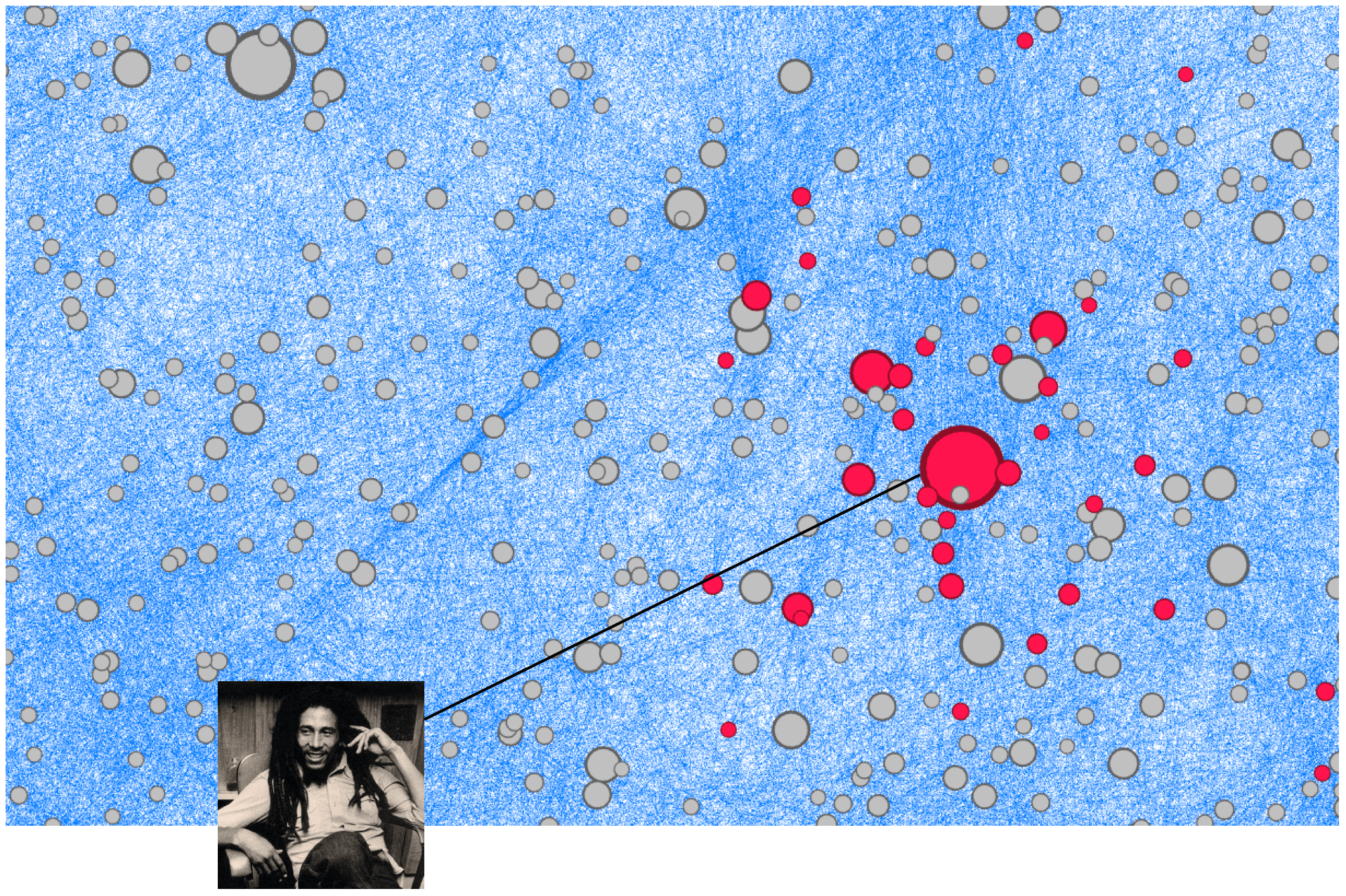
Figure 2. Visualization of some music artists from gravity-inspired graph AE. Nodes are scaled using masses $\tilde{m}_{i}$, and node separation is based on distances in the embedding, using multidimensional scaling and with (Fruchterman and Reingold, 1991). Red nodes correspond to Jamaican reggae artists, appearing in the same neighborhood.

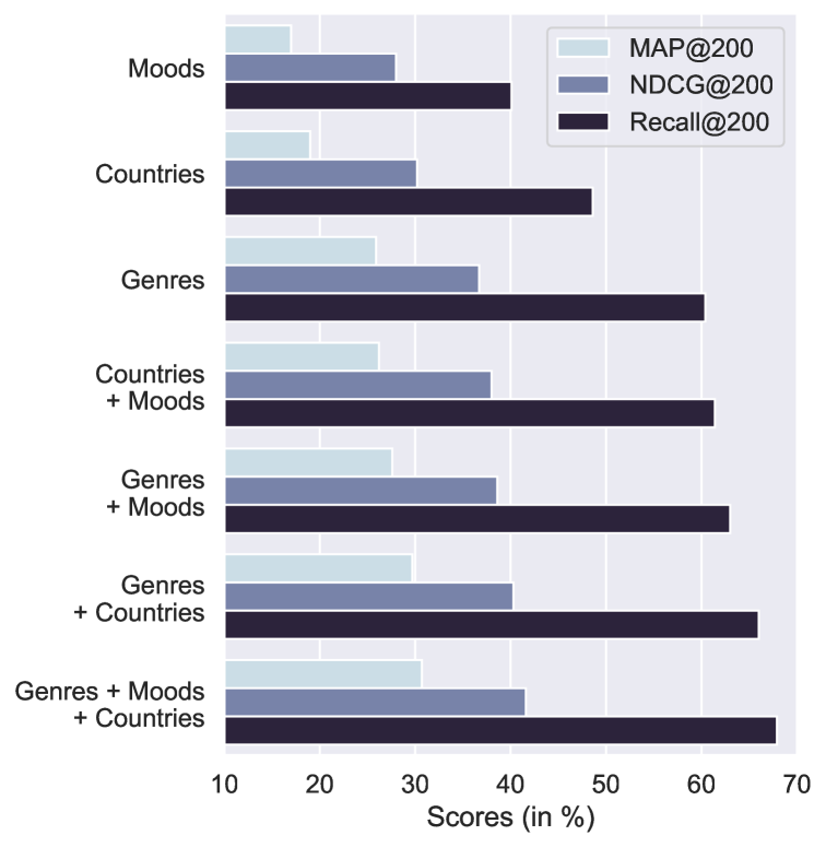
Figure 3. Performances of gravity-inspired graph AE, when only trained from subsets of artist-level attributes, among countries, music genres and moods.

4.3.3. Impact of attributes

So far, all models processed the complete 56-dimensional attribute vectors $x_{i}$, concatenating information on music genres, countries and moods. In Figure 3, we assess the actual impact of each of these descriptions on performances, for our gravity-inspired graph VAE. Assuming only one attribute (genres, countries or moods) is available during training, genres-aware models return the best performances. Moreover, adding moods to country vectors leads to larger gains than adding moods to genre vectors. This could reflect how some of our music genres, such as speed metal, already capture some valence or arousal characteristics. Last, Figure 3 confirms that gathering all three descriptions provides the best performances, corresponding to those reported in Table 1.

4.3.4. Popularity/diversity trade-off

Last, besides performances, the gravity-inspired decoder from equation (4) also enables us to flexibly address popularity biases when ranking similar artists. More precisely:

• Setting $\lambda\rightarrow 0$ increases the relative importance of the influence part of equation (4). Thus, the model will highly rank the most massive nodes. As illustrated in Figure 4, this results in recommending more popular music artists.

• On the contrary, increasing $\lambda$ diminishes the relative importance of masses in predictions, in favor of the actual node proximity. As illustrated in Figure 4, this tends to increase the recommendation of less popular content.

Setting $\lambda=5$ leads to optimal scores in our application (e.g. with a 41.42% NDCG@200 for our AE, v.s. 35.91% and 40.31% for the same model with $\lambda=1$ and $\lambda=20$ respectively). Balancing between popularity and diversity is often desirable for industrial-level recommender systems (Schedl et al., 2018). Gravity-inspired decoders flexibly permit such a balancing.

Table 2. Pearson and Spearman correlation coefficients of masses $\tilde{m}_{i}$ from gravity-inspired graph AE, w.r.t. artist-level reversed popularity ranks (i.e. the higher the more popular) on Deezer and to three node importance measures: in-degree (i.e. sum of edges coming into the node), betweenness centrality (Salha et al., 2019b) and PageRank (Page et al., 1999). Coefficients computed on the training set.

Node-level	Pearson	Spearman
measures	correlation	correlation
Popularity Rank	$0.208$	$0.206$
Popularity Rank by Country	$0.290$	$0.336$
In-degree Centrality	$0.201$	$0.118$
Betweenness Centrality	$0.109$	$0.079$
PageRank Score	$0.272$	$0.153$

Figure 4. Popularity rank of the most popular artist recommended to each test artist, among their top-20. Distributions obtained from gravity-inspired graph AE models with varying hyperparameters $\lambda$.

4.3.5. Possible improvements (on models)

Despite promising results, assuming fixed similarity scores over time might sometimes be unrealistic, as some user preferences could actually evolve. Capturing such changes, e.g. through dynamic graph embeddings, might permit providing even more refined recommendations. Also, during training we kept $k=20$ edges for each artist, while one could consider varying $k$ at the artist level, i.e. adding more (or fewer) edges, depending on the actual musical relevance of each link. One could also compare different metrics, besides mutual information, when constructing the ground-truth graph. Last, we currently rely on a single GCN forward pass to embed cold artists which, while being fast and simple, might also be limiting. Future studies on more elaborated approaches, e.g. to incrementally update GCN weights when new nodes appear, could also improve our current framework.

4.3.6. Possible improvements (on evaluation)

Our evaluation focused on the prediction of ranked lists for cold artists. This permits filling up their ”Fans Also Like/Similar Artists” sections, which was our main goal in this paper. On the other hand, future internal investigations could also aim at measuring to which extent the inclusion of new nodes in the embedding space impacts the existing ranked lists for warm artists. Such an additional evaluation, e.g. via an online A/B test on Deezer, could assess which cold artists actually enter these lists, and whether the new recommendations 1) are more diverse, according to some music or culture-based criteria, and 2) improve user engagement on the service.

5. Conclusion

In this paper, we modeled the challenging cold start similar items ranking problem as a link prediction task, in a directed and attributed graph summarizing information from ”Fans Also Like/Similar Artists” features. We presented an effective framework to address this task, transposing recent advances on gravity-inspired graph autoencoders to recommender systems. Backed by in-depth experiments on artists from the global music streaming service Deezer, we emphasized the practical benefits of our approach, both in terms of recommendation accuracy, of ranking quality and of flexibility. Along with this paper, we publicly release our source code, as well as Deezer data from our experiments. We hope that this release of industrial resources will benefit future research on graph-based cold start recommendation. In particular, we already identified several directions that, in future works, should lead towards the improvement of our approach.

References

- (1)
- Abbasifard et al. (2014) Mohammad Reza Abbasifard, Bijan Ghahremani, and Hassan Naderi. 2014. A Survey on Nearest Neighbor Search Methods. International Journal of Computer Applications 95, 25 (2014).
- Barkan et al. (2019) Oren Barkan, Noam Koenigstein, Eylon Yogev, and Ori Katz. 2019. CB2CF: A Neural Multiview Content-to-Collaborative Filtering Model for Completely Cold Item Recommendations. In 13th ACM Conference on Recommender Systems. 228–236.
- Belkin and Niyogi (2001) Mikhail Belkin and Partha Niyogi. 2001. Laplacian Eigenmaps and Spectral Techniques for Embedding and Clustering. In Advances in Neural Information Processing Systems, Vol. 14. 585–591.
- Bendada et al. (2020) Walid Bendada, Guillaume Salha, and Théo Bontempelli. 2020. Carousel Personalization in Music Streaming Apps with Contextual Bandits. In Fourteenth ACM Conference on Recommender Systems. 420–425.
- Berg et al. (2018) Rianne van den Berg, Thomas N Kipf, and Max Welling. 2018. Graph Convolutional Matrix Completion. KDD Deep Learning Day (2018).
- Briand et al. (2021) Léa Briand, Guillaume Salha-Galvan, Walid Bendada, Mathieu Morlon, and Viet-Anh Tran. 2021. A Semi-Personalized System for User Cold Start Recommendation on Music Streaming Apps. 27th ACM SIGKDD Conference on Knowledge Discovery and Data Mining (KDD).
- Cao et al. (2015) Shaosheng Cao, Wei Lu, and Qiongkai Xu. 2015. Grarep: Learning Graph Representations with Global Structural Information. In CIKM. 891–900.
- Cavendish (1798) Henry Cavendish. 1798. Experiments to Determine the Density of the Earth. Philosophical Transactions of the Royal Society of London 88, 469–526.
- Corbett-Davies and Goel (2018) Sam Corbett-Davies and Sharad Goel. 2018. The Measure and Mismeasure of Fairness: A Critical Review of Fair Machine Learning. arXiv preprint arXiv:1808.00023 (2018).
- Covington et al. (2016) Paul Covington, Jay Adams, and Emre Sargin. 2016. Deep Neural Networks for Youtube Recommendations. In 10th ACM Conf. on Rec. Sys. 191–198.
- Delbouys et al. (2018) Rémi Delbouys, Romain Hennequin, Francesco Piccoli, Jimena Royo-Letelier, and Manuel Moussallam. 2018. Music Mood Detection based on Audio and Lyrics with Deep Neural Net. In 19th International Society for Music Information Retrieval Conference. 370–375.
- Doersch (2016) Carl Doersch. 2016. Tutorial on Variational Autoencoders. arXiv preprint arXiv:1606.05908 (2016).
- Donker (2019) Silvia Donker. 2019. Networking data. A network analysis of Spotify’s socio-technical related artist network. IJMBR 8, 1 (2019), 67–101.
- Epure et al. (2020) Elena V. Epure, Guillaume Salha, Manuel Moussallam, and Romain Hennequin. 2020. Modeling the Music Genre Perception across Language-Bound Cultures. In 2020 Conference on Empirical Methods in Natural Language Processing. 4765–4779.
- Fruchterman and Reingold (1991) Thomas Fruchterman and Edward M Reingold. 1991. Graph drawing by force-directed placement. Software: Practice and exp. 21, 11 (1991), 1129–1164.
- Goodfellow et al. (2016) I. Goodfellow, Y. Bengio, and A. Courville. 2016. Deep Learning. MIT Press.
- Grover et al. (2019) Aditya Grover, Aaron Zweig, and Stefano Ermon. 2019. Graphite: Iterative Generative Modeling of Graphs. In Int. Conf. on Mach. Learn. 2434–2444.
- Hamilton (2020) William L Hamilton. 2020. Graph Representation Learning. Synthesis Lectures on Artifical Intelligence and Machine Learning 14, 3 (2020), 1–159.
- Hamilton et al. (2017) William L. Hamilton, Rex Ying, and Jure Leskovec. 2017. Representation Learning on Graphs: Methods and Applications. IEEE Data Eng. Bul. (2017).
- Hao et al. (2020) Yu Hao, Xin Cao, Yixiang Fang, Xike Xie, and Sibo Wang. 2020. Inductive Link Prediction for Nodes Having Only Attribute Information. In 29th International Joint Conference on Artificial Intelligence. 1209–1215.
- Hasanzadeh et al. (2019) Arman Hasanzadeh, Ehsan Hajiramezanali, Krishna Narayanan, Nick Duffield, Mingyuan Zhou, and Xiaoning Qian. 2019. Semi-Implicit Graph Variational Auto-Encoders. In Advances in Neural Information Processing Systems. 10712–10727.
- He and McAuley (2016) Ruining He and Julian McAuley. 2016. VBPR: Visual Bayesian Personalized Ranking from Implicit Feedback. In 30th AAAI Conf. on Art. Int. 144–150.
- Hsieh et al. (2017) Cheng-Kang Hsieh, Longqi Yang, Yin Cui, Tsung-Yi Lin, Serge Belongie, and Deborah Estrin. 2017. Collaborative Metric Learning. In WWW.
- Huang et al. (2016) Moyuan Huang, Wenge Rong, Tom Arjannikov, Nan Jiang, and Zhang Xiong. 2016. Bi-Modal Deep Boltzmann Machine Based Musical Emotion Classification. In 25th International Conference on Artificial Neural Networks. Springer, 199–207.
- Jain et al. (2020) Gourav Jain, Tripti Mahara, and Kuldeep Narayan Tripathi. 2020. A survey of similarity measures for collaborative filtering-based recommender system. In Soft Computing: Theories and Applications. Springer, 343–352.
- Johnston (2019) Maura Johnston. 2019. How ”Fans Also Like” Works. Blog post on ”Spotify for Artists”: https://artists.spotify.com/blog/how-fans-also-like-works (2019).
- Karatzoglou et al. (2013) Alexandros Karatzoglou, Linas Baltrunas, and Yue Shi. 2013. Learning to Rank for Recommender Systems. In ACM Conference on Rec. Sys. 493–494.
- Kingma and Ba (2015) Diederik P Kingma and Jimmy Ba. 2015. Adam: A Method for Stochastic Optimization. In 3rd International Conference on Learning Representations.
- Kingma and Welling (2014) Diederik P. Kingma and Max Welling. 2014. Auto-Encoding Variational Bayes. In 2nd International Conference on Learning Representations.
- Kipf and Welling (2016) Thomas Kipf and Max Welling. 2016. Variational Graph Auto-Encoders. In NeurIPS Workshop on Bayesian Deep Learning.
- Kipf and Welling (2017) Thomas Kipf and Max Welling. 2017. Semi-Supervised Classification with Graph Convolutional Networks. In 5th Int. Conf. on Learning Representations.
- Kjus (2016) Yngvar Kjus. 2016. Musical Exploration via Streaming services: The Norwegian Experience. Popular Communication 14, 3 (2016), 127–136.
- Koren and Bell (2015) Yehuda Koren and Robert Bell. 2015. Advances in Collaborative Filtering. Recommender Systems Handbook (2015), 77–118.
- Koren et al. (2009) Yehuda Koren, Robert Bell, and Chris Volinsky. 2009. Matrix Factorization Techniques for Recommender Systems. Computer 42, 8 (2009), 30–37.
- Lee et al. (2019) Hoyeop Lee, Jinbae Im, Seongwon Jang, Hyunsouk Cho, and Sehee Chung. 2019. MeLU: Meta-Learned User Preference Estimator for Cold-Start Recommendation. In 25th ACM SIGKDD International Conference on Knowledge Discovery and Data Mining. 1073–1082.
- Lee et al. (2018) Joonseok Lee, Sami Abu-El-Haija, Balakrishnan Varadarajan, and Apostol Natsev. 2018. Collaborative Deep Metric Learning for Video Understanding. In 24th ACM SIGKDD International Conference on Knowledge Discovery and Data Mining. 481–490.
- Li and She (2017) Xiaopeng Li and James She. 2017. Collaborative Variational Autoencoder for Recommender Systems. In 23rd ACM SIGKDD International Conference on Knowledge Discovery and Data Mining. 305–314.
- Liben-Nowell and Kleinberg (2007) David Liben-Nowell and Jon Kleinberg. 2007. The Link Prediction Problem for Social Networks. Journal of the American Society for Information Science and Technology 58, 7 (2007), 1019–1031.
- Liu et al. (2018) Qi Liu, Miltiadis Allamanis, Marc Brockschmidt, and Alexander Gaunt. 2018. Constrained Graph Variational Autoencoders for Molecule Design. Advances in Neural Information Processing Systems, 7806–7815.
- Lu and Zhou (2011) Linyuan Lu and Tao Zhou. 2011. Link Prediction in Complex Networks: A Survey. Physica A: Stat. Mech. and its Applications 390, 6 (2011), 1150–1170.
- Ma et al. (2018) Tengfei Ma, Jie Chen, and Cao Xiao. 2018. Constrained Generation of Semantically Valid Graphs via Regularizing Variational Autoencoders. Advances in Neural Information Processing Systems, 7113–7124.
- Mehrotra et al. (2019) Rishabh Mehrotra, Mounia Lalmas, Doug Kenney, Thomas Lim-Meng, and Golli Hashemian. 2019. Jointly Leveraging Intent and Interaction Signals to Predict User Satisfaction with Slate Recommendations. In The World Wide Web Conference. 1256–1267.
- Newton (1687) Isaac Newton. 1687. Philosophiae Naturalis Principia Mathematica.
- Page et al. (1999) Lawrence Page, Sergey Brin, , and Terry Winograd. 1999. The PageRank Citation Ranking: Bringing Order to the Web. Stanford InfoLab (1999).
- Perozzi et al. (2014) Bryan Perozzi, Rami Al-Rfou, and Steven Skiena. 2014. Deepwalk: Online Learning of Social Representations. In KDD. 701–710.
- Qian et al. (2019) Tieyun Qian, Yile Liang, and Qing Li. 2019. Solving Cold Start Problem in Recommendation with Attribute Graph Neural Networks. arXiv preprint arXiv:1912.12398 (2019).
- Qian et al. (2020) Tieyun Qian, Yile Liang, Qing Li, and Hui Xiong. 2020. Attribute Graph Neural Networks for Strict Cold Start Recommendation. IEEE Transactions on Knowledge and Data Engineering (2020), 1–1.
- Rafailidis and Crestani (2017) Dimitrios Rafailidis and Fabio Crestani. 2017. Learning to Rank with Trust and Distrust in Recommender Systems. In ACM Conf. on Rec. Sys. 5–13.
- Russell (1980) James A Russell. 1980. A Circumplex Model of Affect. Journal of Personality and Social Psychology 39, 6 (1980), 1161.
- Salha et al. (2021) Guillaume Salha, Romain Hennequin, Jean-Baptiste Remy, Manuel Moussallam, and Michalis Vazirgiannis. 2021. FastGAE: Scalable Graph Autoencoders with Stochastic Subgraph Decoding. Neural Networks 142 (2021), 1–19.
- Salha et al. (2019a) Guillaume Salha, Romain Hennequin, Viet Anh Tran, and Michalis Vazirgiannis. 2019a. A Degeneracy Framework for Scalable Graph Autoencoders. In 28th International Joint Conference on Artificial Intelligence. 3353–3359.
- Salha et al. (2020) Guillaume Salha, Romain Hennequin, and Michalis Vazirgiannis. 2020. Simple and Effective Graph Autoencoders with One-Hop Linear Models. In 2020 European Conference on Machine Learning and Principles and Practice of Knowledge Discovery in Databases.
- Salha et al. (2019b) Guillaume Salha, Stratis Limnios, Romain Hennequin, Viet Anh Tran, and Michalis Vazirgiannis. 2019b. Gravity-Inspired Graph Autoencoders for Directed Link Prediction. In 28th ACM International Conference on Information and Knowledge Management. 589–598.
- Schall (2014) Daniel Schall. 2014. Link Prediction in Directed Social Networks. Social Network Analysis and Mining 4, 1 (2014), 157.
- Schedl et al. (2018) Markus Schedl, Hamed Zamani, Ching-Wei Chen, Yashar Deldjoo, and Mehdi Elahi. 2018. Current Challenges and Visions in Music Recommender Systems Research. Int. Journal of Multimedia Information Retrieval 7, 2 (2018), 95–116.
- Shakibian and Charkari (2017) Hadi Shakibian and Nasrollah Charkari. 2017. Mutual Information Model for Link Prediction in Heterogeneous Complex Networks. Scientific Reports 7, 1 (2017), 1–16.
- Srivastava et al. (2014) Nitish Srivastava, Geoffrey Hinton, Alex Krizhevsky, Ilya Sutskever, and Ruslan Salakhutdinov. 2014. Dropout: A Simple Way to Prevent Neural Networks from Overfitting. Journal of Machine Learning Research 15, 1 (2014), 1929–1958.
- Tian et al. (2014) Fei Tian, Bin Gao, Qing Cui, Enhong Chen, and Tie-Yan Liu. 2014. Learning Deep Representations for Graph Clustering. In AAAI. 1293–1299.
- Van Den Oord et al. (2013) Aäron Van Den Oord, Sander Dieleman, and Benjamin Schrauwen. 2013. Deep Content-Based Music Recommendation. In Advances in Neural Information Processing Systems Conference.
- Veličković et al. (2018) Petar Veličković, Guillem Cucurull, Arantxa Casanova, Adriana Romero, Pietro Lio, and Yoshua Bengio. 2018. Graph Attention Networks. In 6th International Conference on Learning Representations.
- Volkovs et al. (2017) Maksims Volkovs, Guang Wei Yu, and Tomi Poutanen. 2017. DropoutNet: Addressing Cold Start in Recommender Systems. In Advances in Neural Information Processing Systems. 4957–4966.
- Wang et al. (2016) Daixin Wang, Peng Cui, and Wenwu Zhu. 2016. Structural Deep Network Embedding. In KDD. 1225–1234.
- Wang et al. (2018) Jizhe Wang, Pipei Huang, Huan Zhao, Zhibo Zhang, Binqiang Zhao, and Dik Lun Lee. 2018. Billion-Scale Commodity Embedding for E-commerce Recommendation in Alibaba. In 24th ACM SIGKDD International Conference on Knowledge Discovery and Data Mining. 839–848.
- Wang et al. (2021) Shoujin Wang, Liang Hu, Yan Wang, Xiangnan He, Quan Z Sheng, Mehmet Orgun, Longbing Cao, Francesco Ricci, and Philip S Yu. 2021. Graph Learning Based Recommender Systems: A Review. In 30th International Joint Conference on Artificial Intelligence.
- Wang et al. (2013) Yining Wang, Liwei Wang, Yuanzhi Li, Di He, Wei Chen, and Tie-Yan Liu. 2013. A Theoretical Analysis of NDCG Ranking Measures. In 26th Annual Conference on Learning Theory, Vol. 8. 6.
- Wu et al. (2020) Shiwen Wu, Fei Sun, Wentao Zhang, and Bin Cui. 2020. Graph Neural Networks in Recommender Systems: A Survey. In arXiv preprint arXiv:2011.02260.
- Wu et al. (2021) Zonghan Wu, Shirui Pan, Fengwen Chen, Guodong Long, Chengqi Zhang, and Philip S Yu. 2021. A Comprehensive Survey on Graph Neural Networks. IEEE Transactions on Neural Networks and Learning Systems 32-1 (2021).
- Ying et al. (2018) Rex Ying, Ruining He, Kaifeng Chen, Pong Eksombatchai, William L Hamilton, and Jure Leskovec. 2018. Graph Convolutional Neural Networks for Web-Scale Recommender Systems. In 24th ACM SIGKDD International Conference on Knowledge Discovery & Data Mining. 974–983.
- Zhang et al. (2019) Jiani Zhang, Xingjian Shi, Shenglin Zhao, and Irwin King. 2019. STAR-GCN: Stacked and Reconstructed Graph Convolutional Networks for Recommender Systems. In 28th International Joint Conference on Artificial Intelligence. 4264–4270.