Implications of oscillating toroidal fields of proto-neutron stars for pulsars and magnetars

Abstract

A fraction of young neutron stars, magnetars, have ultra-strong magnetic fields. Models invoked for their strong fields require highly specific conditions with extreme parameters which are incompatible with the inference that the magnetar birth rate is comparable to the rate of core-collapse supernovae. We suggest that these seemingly contradictory trends can be reconciled if the toroidal magnetic fields are subject to oscillations following the proto-neutron star (PNS) dynamo stage. Depending on the phase of the oscillation at which the oscillations are terminated, the neutron star can have a very high ($\gtrsim 10^{15}\,{\rm G}$) or relatively small ($\sim 10^{14}\,{\rm G}$) toroidal field. As an example, we invoke a shear-driven dynamo model for the generation of PNS magnetic fields and show that the toroidal field indeed exhibits oscillations following the dynamo stage. We argue that these Alfvénic oscillations can lead to the formation of both magnetars and ordinary neutron stars depending on at what phase of the oscillation the fields froze.

1 Introduction

The arguments on the origin of the strong magnetic fields of neutron stars has a long history (Spruit, 2009) which is rekindled by the identification of magnetars i.e., neutron stars with super-strong magnetic fields (Kaspi & Beloborodov, 2017). According to the “fossil field” hypothesis (Woltjer, 1964; Ginzburg, 1964; Ruderman, 1972) the conservation of magnetic flux during the core collapse would lead to the amplification of the magnetic fields. This is commonly assumed as the origin of the magnetic fields of conventional neutron stars. One line of reasoning invokes the “fossil field” hypothesis also for the origin of the magnetic fields of magnetars (Ferrario & Wickramasinghe, 2006, 2008) suggesting they descend from the strong-field tail of the progenitor distribution. Recently, Makarenko et al. (2021) checked this hypothesis by population synthesis methods to find that the model can not explain the distribution of the inferred magnetic fields of the neutron star population given the lack of sufficient number of high-field progenitors.

Another line of reasoning for the origin of neutron star magnetic fields invokes dynamo action (Ruderman & Sutherland, 1973) during the proto-neutron star (PNS) stage and this is widely accepted as the origin of magnetic fields in magnetars (Duncan & Thompson, 1992; Thompson & Duncan, 1993). Numerical simulations (Bonanno et al., 2003, 2005, 2006; Naso et al., 2008; Rheinhardt & Geppert, 2005; Geppert & Rheinhardt, 2006; Raynaud et al., 2020; Lander et al., 2021) suggest that the conditions are favourable for dynamo action if the neutron star starts its life with a period of a few milliseconds (see Bonanno & Urpin, 2008, for a review).

The rather extreme source parameters invoked by the formation scenarios of magnetars (very massive and magnetized progenitors in the case of fossil fields and very rapidly rotating neutron stars in the case of dynamo models) seems to contradict with the relatively high birth rates of magnetars. The core-collapse rate in the Galaxy is $1.9\pm 1.1\,{\rm century^{-1}}$ as implied by the high spectral resolution measurements of ²⁶Al emission at $1808.65\,{\rm keV}$ (Diehl et al., 2006). A more recent estimate is $1.63\pm 0.46\,{\rm century^{-1}}$ (Rozwadowska et al., 2021). The magnetar birth rate is estimated as $0.3\,{\rm century^{-1}}$ (Keane & Kramer, 2008) and $0.23-2\,{\rm century^{-1}}$ (Beniamini et al., 2019). This is only an order of magnitude smaller than or comparable to the core collapse rate suggesting magnetar formation is not as scarce as that implied by the formation scenarios.

Further evidence for the ordinary formation parameters of magnetars is evidenced by the X-ray observations of supernova remnants which do not show evidence that magnetar formation caused larger energy inputs than the formation of standard neutron stars (Vink & Kuiper, 2006). Morever, magnetars appear to have typical space velocities (Deller et al., 2012; Tendulkar et al., 2013) rather than being on the high end tail of the space velocity distribution as required by some magnetar models (Duncan & Thompson, 1992; Thompson & Duncan, 1993). Any model for magnetar formation should reconcile the extreme parameter requirements with the high formation rates, an issue highlighted by Mereghetti et al. (2015).

A defining characteristic of the magnetars is their strong toroidal magnetic field component. This is suggested by theoretical models for their persistent emission (Ferrario & Wickramasinghe, 2008; Perna et al., 2013; Gourgouliatos & Hollerbach, 2018; Igoshev et al., 2021) and the giant flares that could result from its reconfigurations (Thompson & Duncan, 2001). The post-glitch relaxation time-scale of magnetars can be explained by the coupling of vortices to strong toroidal fields (Gügercinoğlu, 2017). Toroidal fields stronger than the dipole fields is hinted by the identification of low-magnetic field “magnetars” (Rea et al., 2010). The dipole (poloidal) fields of the objects inferred from their spin-down is not extreme, yet they show magnetar bursts. The surface fields inferred from phase dependent absorption features (Güver et al., 2011; Tiengo et al., 2013) imply the presence of strong toroidal fields and/or higher multipoles (Ertan & Alpar, 2003; Ekşi & Alpar, 2003; Alpar et al., 2011). Further observational support for the presence of strong toroidal fields in magnetars comes from their free precession indicating they have prolate shapes as would be caused by strong toroidal fields (Makishima et al., 2014).

Here we propose a scenario in which the discrepancy between the magnetar formation scenarios can be reconciled with the high birth rates of magnetars. We assume that both ordinary neutron stars and magnetars have dynamo generated fields with similar parameters. We argue that the toroidal magnetic field, following the dynamo process, oscillates with an amplitude of $B_{\phi,\max}\gtrsim 10^{15}\,{\rm G}$. Depending on the phase of the oscillation at which the fields are frozen, the newborn neutron star will have either super-strong toroidal fields ($B_{\phi}\gtrsim 10^{15}\,{\rm G}$), typical of magnetars, or relatively smaller toroidal magnetic fields ($\sim 10^{14}\,{\rm G}$), typical of pulsars (Gourgouliatos et al., 2013; Gourgouliatos & Hollerbach, 2018). The dynamo process lasts about $\sim 30-40\,{\rm s}$ while the star is subject to the hydromagnetic instabilities (Bonanno et al., 2005). We show, with an already existing simple dynamo model (Wickramasinghe et al., 2014) that the dynamo stage is followed by the oscillations of the toroidal field. Thus, assuming these Alfvénic oscillations are a generic feature of the aftermath of the dynamo stage, slight differences in parameters, not extreme ones, will result with very different toroidal fields and determine whether the proto-neutron star will become a magnetar or a typical neutron star.

The organization of the paper is as follows. In § 2 we introduce the shear-driven dynamo model of Wickramasinghe et al. (2014) proposed originally for the magnetic fields of magnetic white dwarfs, and adopt it to PNS parameters. In § 3 we present the implications of the model for PNSs show the existence of the Alfvénic oscillations following the dynamo stage, and finally in § 4 we discuss the implications of these oscillations for the neutron star populations.

2 Model equations

Very sophisticated dynamo models exist today that solve the PNS dynamo from the first principles i.e., the magnetohydrodynamic equations (see e.g.,  Raynaud et al., 2020). It is not unusual that a dynamo process produces oscillating magnetic fields yet we would like to show this is indeed possible even in a very simple setting. As a simple description of the $\alpha-\Omega$ dynamo operating in PNSs (Duncan & Thompson, 1992; Thompson & Duncan, 1993), we adopt the model proposed by Wickramasinghe et al. (2014) for the magnetic field generation in white dwarfs. This is a shear driven dynamo model effectively describing the turbulent dynamo process driven by differential rotation and convection; it is simple but captures all the essential points of the dynamo process sufficient for our purposes.

Numerical simulations by Braithwaite (2009) suggest that, in order to be stable, the toroidal and poloidal fields should satisfy

$$a\eta^{2}<\eta_{\rm p}<0.8\eta$$ (1)

where $a$ is the buoyancy factor, $\eta\equiv E/|U|$ is the ratio of the magnetic energy to the gravitational potential energy, and $\eta_{\rm p}\equiv E_{\rm P}/|U|$ is the magnetic energy in the poloidal field scaled in the same way. Buoyancy factor is about 10 for main sequence stars (Braithwaite, 2009; Wickramasinghe et al., 2014). It is not easy to obtain the exact value of the buoyancy factor $a$ (Rincon, 2019), but buoyancy is expected to be weaker in the case of neutron stars (Braithwaite, 2009). Accordingly, we choose the buoyancy factor as $a=2$ in presenting most of our results, but we also discuss its effect on the results by varying it in a wide range.

The toroidal field, $B_{\phi}$, is generated from the poloidal field due to the differential rotation, $\Delta\Omega$, within the star, the so called $\Omega$-effect. The field, if it does not satisfy the above constraint given in Equation 1, may also decay with a timescale $\tau_{\phi}$ (see below). The time evolution of the toroidal field is thus given by

$$\frac{dB_{\phi}}{dt}=\Delta\Omega B_{\rm p}-\frac{B_{\phi}}{\tau_{\phi}}~{}.$$ (2)

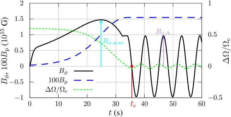
Figure 1: Evolution of the magnetic fields, $B_{\rm p}$ (dashed blue line), $B_{\phi}$ (black solid line) and the differential rotation (dotted green line). Here we assumed $a=2.0$, $\alpha=1.52\times 10^{-4}$, $\Omega=0.9\Omega_{\rm c}$, $B_{\phi}(0)=5\times 10^{11}\,{\rm G}$, $B_{\rm p}(0)=4\times 10^{11}\,{\rm G}$ and $u_{0}=(2/3)\Omega/\Omega_{\rm c}=0.6$. The cyan coloured arrow shows the time at which the toroidal field achieves its maximum value, $B_{\phi,\max}$; the purple arrow shows the amplitude of the toroidal field in the oscillation regime, $B_{\phi,{\rm A}}$ and the red arrow shows the critical time, $t_{\rm c}$ at which the toroidal field vanishes for the first time which we mark as the starting point of the oscillatory phase.

According to Equation 1 the toroidal field is subject to decay if $\eta_{\rm p}<a\eta^{2}$ (Braithwaite, 2009). The total magnetic energy of the star is $E=B^{2}R^{3}/6$ where we assumed the magnetic field to be uniform within the star. Similarly, the magnetic energy in the poloidal field is then $E_{\rm p}=B_{\rm p}^{2}R^{3}/6$. We scale these quantities with the gravitational potential energy of a uniform Newtonian star, $|U|=3GM^{2}/5R$ to determine $\eta$ and $\eta_{\rm p}$ (Wickramasinghe et al., 2014).

The field instabilities, for a non-rotating star, operate on an Alfvén crossing-time scale $\tau_{\rm A}=R/v_{\rm A}$ where $R$ is stellar radius and $v_{\rm A}=B/\sqrt{4\pi\bar{\rho}}$ is the Alfvén velocity and $\bar{\rho}$ is the mean density of star. In the presence of rotation, the growth rate of the instabilities are reduced by a factor of $\Omega\tau_{\rm A}/2\mathrm{\pi}$ (Pitts & Tayler, 1985). Thus $\tau_{\phi}$ is given by:

$$\tau_{\phi}=\begin{cases}\infty&\text{ if }\eta_{\rm p}>a\eta^{2}\\ \max\left(1,\frac{\Omega\tau_{\rm A}}{2\mathrm{\pi}}\right)\tau_{\mathrm{A}}&\text{ otherwise }\end{cases}$$ (3)

where $\Omega$ is the stellar angular velocity.

The poloidal field is generated from the toroidal field in the presence of cyclonic convection by the $\alpha$-effect while it also relaxes on a timescale $\tau_{\rm p}$ (see below) in case the field configuration is unstable. We thus write

$$\frac{dB_{\rm p}}{dt}=\alpha\frac{B_{\phi}}{\tau_{\phi}}-\frac{B_{\rm p}}{\tau_{\rm p}}~{}.$$ (4)

where $\alpha$ is the efficiency factor. The time-scale for the decay of the poloidal field is given by

$$\tau_{\rm P}=\begin{cases}\infty&\text{ if }0.8\eta>\eta_{\rm P}\\ \max\left(1,\frac{\Omega\tau_{\rm A}}{2\pi}\right)\tau_{\rm A}&\text{ otherwise. }\end{cases}$$ (5)

We have seen that, to obtain poloidal magnetic fields of order $10^{14}\,{\rm G}$ we must choose $\alpha=1\times 10^{-3}$.

The magnetic torque inside the star tends to decrease the differential rotation of the star. For this, we again employ the prescription by Wickramasinghe et al. (2014)

$$I\frac{d\Delta\Omega}{dt}=-B_{\phi}B_{\rm p}R^{3}$$ (6)

where $I=\gamma MR^{2}$ is the moment of inertia. We have taken $\gamma=0.35$ for a PNS of $1.4M_{\sun}$.

The dynamo process will proceed for about $40\,{\rm s}$ (Raynaud et al., 2020). We do not explicitly include the physics of what terminates the dynamo process. This would require us to include the effects of neutrino cooling and other less constrained physics into the model. Yet it is only necessary to note that the termination of the process is governed by conditions quite independent the above described dynamics.

3 Results

We have numerically solved Equations (2)-(6) with the Runge-Kutta method. We set $M=1.4M_{\sun}$ and $R=40\,{\rm km}$ appropriate for a PNS. Accordingly, we have calculated the break-up speed $\Omega_{\rm c}=\sqrt{GM/R^{3}}$ and assumed $\Omega=0.9\Omega_{\rm c}\simeq 1534\,{\rm rad/s}$. We have also scaled the differential rotation as $u\equiv\Delta\Omega/\Omega_{\rm c}$ and assumed $u(t=0)=(2/3)\Omega/\Omega_{\rm c}=0.6$. We assumed that the PNS inherits a small field from the progenitor by flux freezing. We have set $B_{\rm p}(t=0)=4\times 10^{11}\,{\rm G}$ and $B_{\phi}(t=0)=5\times 10^{11}\,{\rm G}$. We have also studied the implications of changing all these parameters. Note that the angular velocity we employ is very high in the sense that when the PNS settles to be a neutron star of $12\,{\rm km}$ it should loose a lot of angular momentum to remain below the corresponding break-up speed.

In Figure 1 we show the evolution of the poloidal and toroidal magnetic fields, and the differential rotation within the star. The initial evolution of the fields and differential rotation match with that given in Wickramasinghe et al. (2014). In this regime the toroidal field grows in time from the seed field until it reaches a maximum value, $B_{\phi,\max}$ and then decays slightly while the poloidal field grows monotonically and approaches the value at which it will saturate, $B_{\rm p,\infty}$ due to the non-linear feedback of $B$ on $\Delta\Omega$.

3.1 The oscillatory stage

For all the wide range of parameters we solved the system, we observe that the initial dynamo stage is followed by an oscillatory stage in which the toroidal field and the differential rotation oscillate. This oscillatory stage is not depicted and discussed by Wickramasinghe et al. (2014) probably because it is not a part of the dynamo stage. As seen from Figure 1 the oscillation of the toroidal field lags the oscillation of the differential rotation within the star by ${\rm\pi}/2\,{\rm rad}$. We define $t_{\rm c}$ as the critical time at which the toroidal field vanishes for the first time (shown with the red arrow in the figure).

We can understand the oscillatory behaviour of the toroidal field and differential rotation analytically as follows: We see from the numerical simulation data that in the oscillatory regime $\tau_{\phi}\rightarrow\infty$ at all times. In the same regime $\tau_{\rm p}$ also is infinite except for the brief episodes while $B_{\phi}$ is vanishingly small i.e., when $B_{\phi}$ is changing sign. This does not change the dynamics. The dynamical equations given in (2) and (4) simplify and we write them as

$$\dot{B}_{\phi}=\Omega_{\rm c}uB_{\rm p}~{},\qquad\dot{B}_{\rm p}=0~{},\qquad\dot{u}=-\frac{R^{3}}{I\Omega_{\rm c}}B_{\phi}B_{\rm p}$$ (7)

where we defined $u\equiv\Delta\Omega/\Omega_{\rm c}$ as the dimensionless differential rotation and used the dot notation for the time derivatives. Taking the derivative of the first and the third equations above, and using the middle one, we obtain

$$\ddot{B}_{\phi}=-\omega^{2}B_{\phi}~{},\qquad\ddot{u}=-\omega^{2}u$$ (8)

where $\omega\equiv\sqrt{R^{3}/I}\,B_{\rm p}$. With appropriate scaling the angular frequency of the oscillations can be written as

$$\omega=0.8\,{\rm rad~{}s^{-1}}\,\left(\frac{R}{40\,{\rm km}}\right)^{3/2}\left(\frac{I}{10^{46}\,{\rm g~{}cm^{2}}}\right)^{-1/2}\left(\frac{B_{\rm p}}{10^{12}\,{\rm G}}\right)~{}.$$ (9)

Equation 8 shows that the toroidal field, $B_{\phi}$, and the differential rotation $\Delta\Omega$ obey simple harmonic oscillator equations. Setting $u=u_{\max}\cos\omega t$ and $B_{\phi}=B_{\phi\max}\sin\omega t$ and using these in the first equation of (7) we get

$$B_{\rm p}=\frac{\omega B_{\phi\max}}{u_{\max}\Omega_{\rm c}}~{},$$ (10)

but this does not determine the value of $B_{\rm p}$ since, by using $\omega=\sqrt{R^{3}/I}\,B_{\rm p}$, we obtain

$$B_{\phi\max}=\sqrt{\frac{I}{R^{3}}}\Omega_{\rm c}u_{\max}$$ (11)

i.e., $B_{\rm p}$ cancels from both sides. Equation 11 shows that the amplitudes of the oscillation of $B_{\phi}$ is proportional to $u_{\max}$ and the proportionality constant is determined purely by the mass and radius of the pro-neutron star, rather than the initial spin.

Although $\dot{B}_{\rm p}=0$ implies $B_{\rm p}=\alpha\tau_{\rm p}B_{\phi}/\tau_{\phi}$, this can not be used to determine the value of $B_{\rm p}$ since, except for when $B_{\phi}\simeq 0$, both $\tau_{\rm p}$ and $\tau_{\phi}$ are infinite and so the ratio $\tau_{\rm p}/\tau_{\phi}$ is indeterminate. For the same reason, we can not argue that $B_{\rm p}$ should be oscillating with $B_{\phi}$. This also would be contradicting with $\dot{B}_{\rm p}=0$. Thus, in the following, we seek for how $B_{\rm p}$ depends on the parameters we have chosen.

3.2 Dependences on the parameters

We have investigated the effect of the parameters of the model on the resulting fields and the time at which oscillatory behaviour commences, $t_{\rm c}$. We have found that higher angular velocity of the PNS, higher initial value of the differential rotation, higher values of the efficiency parameter $\alpha$, higher value of the average density, $\bar{\rho}$, higher initial poloidal and toroidal fields and lower values of buoyancy parameters $a$ lead to shorter $t_{\rm c}$ values (see the Online Supplementary Material). We hope these results can address under what conditions more advanced simulations of the PNS dynamo can exhibit oscillating toroidal magnetic fields.

4 Discussion

We attempted to address the important problem mentioned in the excellent review by Mereghetti et al. (2015): there is discrepancy between the extreme parameters as required by magnetar models and the high birthrates of magnetars among the rate of core collapse in Galaxy. We suggested that this problem could be resolved if the toroidal magnetic field exhibits oscillatory behaviour following the dynamo stage. For a quantitative illustration of the idea, we considered a simple dynamo model which was originally introduced for white dwarfs by Wickramasinghe et al. (2014). We found that the model indeed predicts Alfvénic oscillations for the toroidal fields.

Using the simple dynamo model of Wickramasinghe et al. (2014) we have seen that the period of the oscillations of the toroidal field is $T=2{\rm\pi}/\omega\simeq 7.85\,{\rm s}\,B_{12}^{-1}$ where $B_{12}$ is the magnitude of the saturation value of the poloidal field, $B_{\rm p,\infty}$ in units of $10^{12}\,{\rm G}$.

The oscillatory behaviour for the toroidal field has important implications for the origin of magnetic fields of neutron stars. Depending on the phase at which the oscillations terminate, a PNS can have a strong or weak toroidal field. If the PNS has a strong toroidal field ($\gtrsim 10^{15}\,{\rm G}$), the nascent neutron star that forms upon its collapse will also have a strong toroidal field and it will eventually ($t\sim 10^{2}-10^{4}\,{\rm yr}$) appear as a magnetar. If the dynamo terminates when the toroidal field is not near the maximum, the nascent neutron star to be formed from the collapse of the PNS will have a smaller toroidal field ($\sim 10^{14}\,{\rm G}$) and likely appear as an ordinary neutron star in its later life. At what phase the fields are frozen will be set by the processes damping these Alfvénic oscillations and is beyond the scope of the present paper. Yet we argue that, in order that the resulting populations are compatible with the observed ratio of the pulsars to magnetars, magnetars should be associated with only a small fraction of the phase of oscillation near the peak.

The poloidal magnetic field generated with the parameters employed here, $B_{\rm p,\infty}\sim 10^{13}\,{\rm G}$) is comparable with high magnetic field tail of rotationally-powered pulsars and low-magnetic field magnetars, but rather small compared to the dipole fields of most of the magnetars as inferred from their spin-down. Here we assumed that what makes a magnetar different than other neutron stars is their toroidal magnetic fields. This is hinted by the existence of low-magnetic field magnetars and magnetar behaviour observed from some rotationallypowered pulsars. In the Appendix we show that higher poloidal fields can be obtained by higher values of the efficiency parameter $\alpha$ and with higher average densities i.e. for higher mass proto-neutron stars.

Data availability

No new data were analysed in support of this paper.

Appendix A Supplementary material

In the main manuscript we have chosen specific parameters for the proto-neutron star (PNS). Specifically, we set mass and radius of the PNS as $M=1.4M_{\bigodot}$ and $R=40\,{\rm km}$. We assumed $\Omega=0.9\Omega_{\rm c}\simeq 1534\,{\rm rad/s}$ where $\Omega_{\rm c}=\sqrt{GM/R^{3}}$ is the break-up speed. We have also scaled the differential rotation as $u\equiv\Delta\Omega/\Omega_{\rm c}$ and assumed $u(t=0)=(2/3)\Omega/\Omega_{\rm c}=0.6$. We assumed that the proto-neutron star inherits a small field from the progenitor by flux freezing. We have set $B_{\rm p}(t=0)=4\times 10^{11}\,{\rm G}$ and $B_{\phi}(t=0)=5\times 10^{11}\,{\rm G}$.

In this supplementary material we study the implications of changing all these parameters.

A.1 Dependence on the angular velocity

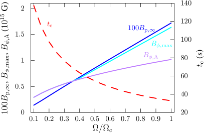
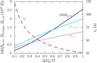
Figure 2: Effect of angular velocity $\Omega$ (left panel) and the differential rotation (right panel) on the saturation value of the poloidal field, $B_{\rm p}$ (coloured blue in the electronic version); the maximum value of the toroidal field, $B_{\phi,\max}$ (coloured cyan in the electronic version); the amplitude of the oscillations of the toroidal field $B_{\phi,{\rm A}}$ (coloured purple in the electronic version), and the critical time, $t_{\rm c}$, at which $B_{\phi}$ starts oscillating (coloured red in the electronic version). Here $a=2$, $\alpha=1.52\times 10^{-4}$, $B_{\phi}(0)=5\times 10^{11}\,{\rm G}$, $B_{\rm p}(0)=4\times 10^{11}\,{\rm G}$ and $u_{0}=(2/3)\Omega/\Omega_{\rm c}$.

To determine the dependence of $B_{\rm p}$ on the angular velocity of the star, we varied the angular velocity from $\Omega/\Omega_{\rm c}=0.1$ to $\Omega/\Omega_{\rm c}=1.0$. The lower end of this angular velocity range for the proto-neutron star would still lead to a very high rotation rate for the neutron star when the radius shrinks from $40\,{\rm}$ to $12\,{\rm km}$ assuming angular momentum conservation.

Obviously, the differential rotation within the star can not be larger than the angular velocity of the star. Accordingly, we set the initial value of the differential rotation to 2/3 of the angular velocity of the star in each case. In the following subsection we analyzed the effects of varying this constant.

We find that the saturation value of the poloidal field, $B_{\rm p,\infty}$, and the amplitude of the toroidal field in the oscillatory phase, $B_{\phi,{\rm A}}$ increases linearly with the angular velocity as shown in the left panel of Figure 2. The results in the figure can be described as

$$\frac{B_{\rm p,\infty}}{10^{13}\,{\rm G}} =1.75\left(\frac{\Omega}{\Omega_{\rm c}}\right)-0.0263,$$ (12)

$$\frac{B_{\phi,\max}}{10^{15}\,{\rm G}} =1.628\left(\frac{\Omega}{\Omega_{\rm c}}\right)-0.0075\quad\mbox{for }\frac{\Omega}{\Omega_{\rm c}}\geq 0.4~{}.$$ (13)

For $\Omega/\Omega_{\rm c}<0.4$ the toroidal field attains its maximum value only at the end of the initial transient stage and this maximum value matches with the amplitude of oscillations. It can also be seen that the amplitude of the toroidal field, $B_{\phi,{\rm A}}$ increases with $\Omega$ as a power law

$$\frac{B_{\phi,{\rm A}}}{10^{15}\,{\rm G}}=1.02\left(\frac{\Omega}{\Omega_{\rm c}}\right)^{0.523}~{}.$$ (14)

We also determine how the critical time, $t_{\rm c}$, which marks the beginning of the oscillatory behaviour, depends on the angular velocity, $\Omega$. We find that $t_{\rm c}$ decreases as a power-law

$$t_{\rm c}=34.8\left(\frac{\Omega}{\Omega_{\rm c}}\right)^{-0.62}$$ (15)

(see the left panel of Figure 2).

A.2 Dependence on the initial value of the differential rotation

The inital value of the differential rotation (in units of angular velocity) also increases the final values of the fields $B_{\rm p}$, $B_{\phi,\max}$ and $B_{\phi,{\rm A}}$, and lowers $t_{\rm c}$ as shown in the right panel of Figure 2).

By fitting the results of several numerical simulations we find

$$\frac{B_{\rm p,\infty}}{10^{13}\,{\rm G}} =2.5275(\Delta\Omega_{0}/\Omega)^{1.2}~{};$$ (16)

$$\frac{B_{\phi,\max}}{10^{15}\,{\rm G}} =1.975(\Delta\Omega_{0}/\Omega)^{0.72}~{};$$ (17)

$$\frac{B_{\phi,{\rm A}}}{10^{15}\,{\rm G}} =1.233(\Delta\Omega_{0}/\Omega)^{0.60}~{};$$ (18)

$$t_{\rm c} =27.22(\Delta\Omega_{0}/\Omega)^{-0.67}~{}.$$ (19)

A.3 Dependence on the efficiency parameter, $\alpha$

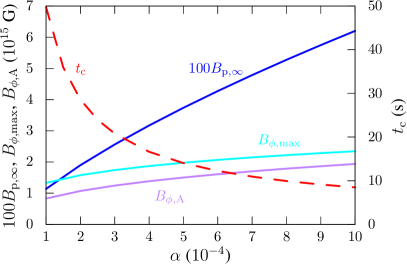
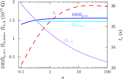
Figure 3: (left panel) Effect of efficiency parameter $\alpha$ on the generated poloidal field, $B_{\rm p}$ (coloured blue in the electronic version); the maximum value of the toroidal field, $B_{\phi,\max}$ (coloured cyan in the electronic version); the amplitude of the oscillations of the toroidal field $B_{\phi,{\rm A}}$ (coloured purple in the electronic version), and the critical time, $t_{\rm c}$, at which $B_{\phi}$ starts oscillating (coloured red in the electronic version). Here $\Omega=0.9\Omega_{\rm c}$, $B_{\phi}(0)=5\times 10^{11}\,{\rm G}$, $B_{\rm p}(0)=4\times 10^{11}\,{\rm G}$ and $u_{0}=0.6$. (Right panel) Effect of buoyancy factor, $a$, on the saturated value of the poloidal field, $B_{\rm p}$ (solid line coloured blue in the electronic version) and the critical time, $t_{\rm c}$, at which $B_{\phi}$ starts oscillating (dashed line coloured red in the electronic version). Here $\Omega=0.9\Omega_{\rm c}$, $\alpha=1.52\times 10^{-4}$, $B_{\phi}(0)=5\times 10^{11}\,{\rm G}$ and $u_{0}=0.6$.

We also analysed the results of simulations at which the efficiency parameter $\alpha$ is varied in the range $(1-10)\times 10^{-4}$. We found that the saturation value of the poloidal field, $B_{\rm p,\infty}$, increases with $\alpha$ as shown in the left panel of Figure 3. We also found that the maximum value of the toroidal field, $B_{\phi,\max}$, and the amplitude of the toroidal field, $B_{\phi,{\rm A}}$ increases less steeply with $\alpha$. The results can be modeled as

$$\frac{B_{\rm p,\infty}}{10^{13}\,{\rm G}} =1.138(\alpha/10^{-4})^{0.7375}~{};$$ (20)

$$\frac{B_{\phi,\max}}{10^{15}\,{\rm G}} =1.329(\alpha/10^{-4})^{0.2462}~{};$$ (21)

$$\frac{B_{\phi,{\rm A}}}{10^{15}\,{\rm G}} =0.828(\alpha/10^{-4})^{0.3695}~{};$$ (22)

$$t_{\rm c} =49.13\,{\rm s}\,(\alpha/10^{-4})^{-0.7693}~{}.$$ (23)

A.4 Dependence on the buoyancy parameter, $a$

We show the effect of buoyancy factor $a$ on $B_{\rm p,\infty}$, $B_{\phi,\max}$, $B_{\phi,{\rm A}}$ and $t_{\rm c}$ in the right panel of Figure 3. As the buoyancy factor increases, $B_{\rm p,\infty}$ and $t_{\rm c}$ increases, but this is a very weak dependence. We see that $B_{\phi,\max}$ remains constant for $a>0.3$. For $a<0.3$ the toroidal field does not attain a maximum value before the oscillatory phase. Only $B_{\phi,{\rm A}}$ depends strongly on the buoyancy parameter and we model it as

$$\frac{B_{\phi,{\rm A}}}{10^{15}\,{\rm G}}=1.135\,a^{-0.242}~{}.$$ (24)

A.5 Dependence on the average density of the proto-neutron star

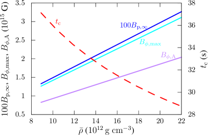
Figure 4: Effect of the density of the proto-neutron star, $\bar{\rho}$ on the saturated value of the poloidal field, $B_{\rm p}$, (coloured blue in the electronic version); the maximum value of the toroidal field, $B_{\phi,\max}$ (coloured cyan in the electronic version); the amplitude of the oscillations of the toroidal field $B_{\phi,{\rm A}}$ (coloured purple in the electronic version), and the critical time, $t_{\rm c}$, at which $B_{\phi}$ starts oscillating (coloured red in the electronic version). Here $a=2$, $\Omega=0.9\Omega_{\rm c}$, $\alpha=1.52\times 10^{-4}$, $B_{\phi}(0)=5\times 10^{11}\,{\rm G}$ and $u_{0}=0.6$.

We have investigated the effect of the average density of the proto-neutron star on $B_{\rm p,\infty}$, $B_{\phi,\max}$, $B_{\phi,{\rm A}}$ and $t_{\rm c}$ (see Figure 4). We find that the fields increase linearly with the average density while $t_{\rm c}$ decreases with a power-law. Results of the parameter scan can be summarized as

$$\frac{B_{\rm p,\infty}}{10^{13}\,{\rm G}} =0.148\bar{\rho}_{12}+0.0107~{};$$ (25)

$$\frac{B_{\phi,\max}}{10^{15}\,{\rm G}} =0.141\bar{\rho}_{12}+0.006~{};$$ (26)

$$\frac{B_{\phi,{\rm A}}}{10^{15}\,{\rm G}} =0.093\bar{\rho}_{12}+0.0033~{};$$ (27)

$$t_{\rm c} =69.09\bar{\rho}_{12}^{-0.283}$$ (28)

where $\bar{\rho}_{12}=\bar{\rho}/10^{12}\,{\rm g~{}cm^{-3}}$.

A.6 Dependence on the initial value of the fields

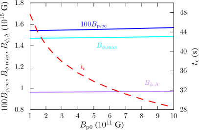
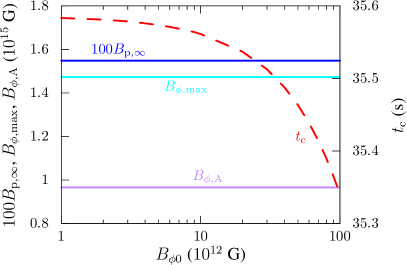
Figure 5: Effect of initial poloidal field $B_{\rm p}(0)$ (left panel) and toroidal field (right panel) on the results. The saturated value of the poloidal field, $B_{\rm p,\infty}$ (coloured blue in the electronic version) and the critical time, $t_{\rm c}$, at which $B_{\phi}$ starts oscillating (dashed line coloured red in the electronic version). Here $a=2$, $\Omega=0.9\Omega_{\rm c}$, $\alpha=1.52\times 10^{-4}$, $B_{\phi}(0)=5\times 10^{11}\,{\rm G}$ and $u_{0}=0.6$.

We also checked the dependence of $B_{\rm p}$, $B_{\phi,\max}$, $B_{\phi,{\rm A}}$ and $t_{\rm c}$ on the initial value of the poloidal and toroidal fields, $B_{\rm p0}$ and $B_{\phi 0}$. The result for this is shown in Figure 5. We see that the fields depend very weakly on $B_{\rm p0}$ while the critical time drops with the initial poloidal field as $t_{\rm c}=48.14(B_{\rm p0}/10^{11}\,{\rm G})^{-0.2236}$. The critical time depends very weakly on the initial value of the toroidal field. In short, the initial value of the poloidal and toroidal fields are not important in setting the final values of the fields in the dynamo process while higher initial values lead to earlier commence of the oscillatory behaviour.

We note that the poloidal field is two orders of magnitude smaller than the toroidal field. The poloidal field will be enhanced, by flux conservation, upon the collapse of the proto-neutron star to the typical size of a neutron star. The enhancement will be $(40\,{\rm km}/12\,{\rm km})^{2}\simeq 11.1$ times $B_{\rm p,\infty}$. The toroidal field will not be affected by the collapse. The gravitational potential energy $|3GM^{2}/5R$ will also be enhanced by a factor of $40\,{\rm km}/12\,{\rm km}\simeq 3.3$

References

- Alpar et al. (2011) Alpar M. A., Ertan Ü., Çalışkan Ş., 2011, ApJ, 732, L4
- Beniamini et al. (2019) Beniamini P., Hotokezaka K., van der Horst A., Kouveliotou C., 2019, MNRAS, 487, 1426
- Bonanno et al. (2003) Bonanno A., Rezzolla L., Urpin V., 2003, A&A, 410, L33
- Bonanno & Urpin (2008) Bonanno A., Urpin V., 2008, in Exotic States of Nuclear Matter Protoneutron Star Dynamo: Theory and Observations. pp 155–158
- Bonanno et al. (2005) Bonanno A., Urpin V., Belvedere G., 2005, A&A, 440, 199
- Bonanno et al. (2006) Bonanno A., Urpin V., Belvedere G., 2006, A&A, 451, 1049
- Braithwaite (2009) Braithwaite J., 2009, MNRAS, 397, 763
- Deller et al. (2012) Deller A. T., Camilo F., Reynolds J. E., Halpern J. P., 2012, ApJ, 748, L1
- Diehl et al. (2006) Diehl R., Halloin H., Kretschmer K., Lichti G. G., Schönfelder V., Strong A. W., von Kienlin A., Wang W., Jean P., Knödlseder J., Roques J.-P., Weidenspointner G., Schanne S., Hartmann D. H., Winkler C., Wunderer C., 2006, Nature, 439, 45
- Duncan & Thompson (1992) Duncan R. C., Thompson C., 1992, ApJ, 392, L9
- Ekşi & Alpar (2003) Ekşi K. Y., Alpar M. A., 2003, ApJ, 599, 450
- Ertan & Alpar (2003) Ertan Ü., Alpar M. A., 2003, ApJ, 593, L93
- Ferrario & Wickramasinghe (2006) Ferrario L., Wickramasinghe D., 2006, MNRAS, 367, 1323
- Ferrario & Wickramasinghe (2008) Ferrario L., Wickramasinghe D., 2008, MNRAS, 389, L66
- Geppert & Rheinhardt (2006) Geppert U., Rheinhardt M., 2006, A&A, 456, 639
- Ginzburg (1964) Ginzburg V. L., 1964, Soviet Physics Doklady, 9, 329
- Gourgouliatos et al. (2013) Gourgouliatos K. N., Cumming A., Reisenegger A., Armaza C., Lyutikov M., Valdivia J. A., 2013, MNRAS, 434, 2480
- Gourgouliatos & Hollerbach (2018) Gourgouliatos K. N., Hollerbach R., 2018, ApJ, 852, 21
- Gügercinoğlu (2017) Gügercinoğlu E., 2017, MNRAS, 469, 2313
- Güver et al. (2011) Güver T., Göǧüş E., Özel F., 2011, MNRAS, 418, 2773
- Igoshev et al. (2021) Igoshev A. P., Hollerbach R., Wood T., Gourgouliatos K. N., 2021, Nature Astronomy, 5, 145
- Kaspi & Beloborodov (2017) Kaspi V. M., Beloborodov A. M., 2017, ARA&A, 55, 261
- Keane & Kramer (2008) Keane E. F., Kramer M., 2008, MNRAS, 391, 2009
- Lander et al. (2021) Lander S. K., Haensel P., Haskell B., Zdunik J. L., Fortin M., 2021, MNRAS, 503, 875
- Makarenko et al. (2021) Makarenko E. I., Igoshev A. P., Kholtygin A. F., 2021, MNRAS
- Makishima et al. (2014) Makishima K., Enoto T., Hiraga J. S., Nakano T., Nakazawa K., Sakurai S., Sasano M., Murakami H., 2014, PRL, 112, 171102
- Mereghetti et al. (2015) Mereghetti S., Pons J. A., Melatos A., 2015, Space Science Reviews, 191, 315
- Naso et al. (2008) Naso L., Rezzolla L., Bonanno A., Paternò L., 2008, A&A, 479, 167
- Perna et al. (2013) Perna R., Viganò D., Pons J. A., Rea N., 2013, MNRAS, 434, 2362
- Pitts & Tayler (1985) Pitts E., Tayler R. J., 1985, MNRAS, 216, 139
- Raynaud et al. (2020) Raynaud R., Guilet J., Janka H.-T., Gastine T., 2020, Science Advances, 6, eaay2732
- Rea et al. (2010) Rea N., Esposito P., Turolla R., Israel G. L., Zane S., Stella L., Mereghetti S., Tiengo A., Götz D., Göğüş E., Kouveliotou C., 2010, Science, 330, 944
- Rheinhardt & Geppert (2005) Rheinhardt M., Geppert U., 2005, A&A, 435, 201
- Rincon (2019) Rincon F., 2019, Journal of Plasma Physics, 85, 205850401
- Rozwadowska et al. (2021) Rozwadowska K., Vissani F., Cappellaro E., 2021, Nature Astronomy, 83, 101498
- Ruderman (1972) Ruderman M., 1972, ARA&A, 10, 427
- Ruderman & Sutherland (1973) Ruderman M. A., Sutherland P. G., 1973, Nature Physical Science, 246, 93
- Spruit (2009) Spruit H. C., 2009, in Strassmeier K. G., Kosovichev A. G., Beckman J. E., eds, Cosmic Magnetic Fields: From Planets, to Stars and Galaxies Vol. 259, The source of magnetic fields in (neutron-) stars. pp 61–74
- Tendulkar et al. (2013) Tendulkar S. P., Cameron P. B., Kulkarni S. R., 2013, ApJ, 772, 31
- Thompson & Duncan (1993) Thompson C., Duncan R. C., 1993, ApJ, 408, 194
- Thompson & Duncan (2001) Thompson C., Duncan R. C., 2001, ApJ, 561, 980
- Tiengo et al. (2013) Tiengo A., Esposito P., Mereghetti S., Turolla R., Nobili L., Gastaldello F., Götz D., Israel G. L., Rea N., Stella L., Zane S., Bignami G. F., 2013, Nature, 500, 312
- Vink & Kuiper (2006) Vink J., Kuiper L., 2006, MNRAS, 370, L14
- Wickramasinghe et al. (2014) Wickramasinghe D. T., Tout C. A., Ferrario L., 2014, MNRAS, 437, 675
- Woltjer (1964) Woltjer L., 1964, ApJ, 140, 1309