Pair Cascades at the Edge of the Broad- Line Region Shaping the Gamma-Ray Spectrum of 3C 279

Abstract

The blazar 3C 279 emits a flux of gamma-rays that is variable on timescales as short as the light-crossing time across the event horizon of its central black hole. It is commonly reported that the spectral energy distribution (SED) does not show signs of pair attenuation due to interactions of the gamma rays with ambient ultraviolet photons, concluding that the gamma rays must originate from substructures in the jet outside of the broad-line region (BLR). We address the spectral signature imprinted by atomic emission lines on the gamma-ray spectrum produced by an inverse-Compton pair cascade in the photon field of the BLR. We determine with high precision the gamma-ray SED of 3C 279 using Fermi Large Area Telescope data from MJD 58129–58150 and simulate the pair cascade spectrum for three different injection terms. Satisfactory fits to the observational data are obtained. The obtained SED shows features imprinted by pair production on atomic emission line photons due to optically thick radiation transport, but lacking further exponential attenuation expected if the emission region would lie buried deep within the BLR. The SED of 3C 279 is consistent with an inverse-Compton pair cascade spectrum without exponential external pair absorption. Our findings support the view that the gamma-ray emission in 3C 279 originates from the edge of the BLR.

2021

1 Introduction

Since the first detection of gamma-ray emission from the flat-spectrum radio quasar (FSRQ) 3C 279 in 1991 by the energetic gamma ray experiment telescope (EGRET) (Hartman et al. 1992), the location and extent of its originating region is debated. Recently, the inner jet of 3C 279 was imaged at millimeter wavelengths with an unprecedented angular resolution of $\approx 20\,\mu\rm as$ (Kim et al. 2020). The resolution in the gamma-ray regime is, however, orders of magnitude bigger than the resolution necessary to directly dissect the morphological structure of the active galactic nucleus (AGN). Thus, only indirect arguments can be brought forth in the discussion on the nature of the emission region of gamma rays from blazars.

The effect of absorption on the observed gamma-ray spectra of quasars due to pair production (PP) in collisions of their GeV photons with photons from the ultraviolet (UV) to X-ray radiation field within the broad emission line region (BLR) has been studied by Donea & Protheroe (2003) and by Liu & Bai (2006). The latter authors constructed a spherical, shell-like BLR model and took observed emission lines as well as continuum blackbody radiation into account. By determining the pair-absorption (= absorption of photons due to PP) optical depth, they concluded that detection of radiation from $10\,\rm GeV$ to some $100\,\rm GeV$ from 3C 279 (and FSRQs in general) would imply emission from a distance of several $10^{15}\,\rm m$ away from the central object, hence not from inside the BLR. If radiation above $10\,\rm{GeV}$ was emitted inside the BLR, it would be completely absorbed.

A similar approach was pursued by Reimer (2007) using a double-absorber model and including redshift dependence, by Tavecchio & Mazin (2009) and Tavecchio & Ghisellini (2012), who used the photoionization code Cloudy, and by Britto et al. (2015), who used the six strongest UV lines, to model BLR spectra of 3C 279 and optical depths, which are found to be $\approx 10$ above few tens of $\rm GeV$ and for emission from within the BLR. Less severe limits were found by Böttcher & Els (2016), who determined the optical depth of a spherical, shell-like BLR of 3C 279 to be $>1$ only inside the inner boundary and only for energies $>50\,\rm GeV$.

In their extensive variability study of the brightest flares of 3C 279 and other Fermi-detected FSRQs, Meyer et al. (2019) found no significant imprint of absorption, and determine the minimum distance of the emission region to several $10^{14}\,\rm m$, in agreement with estimates based on variability and on the comparison of cooling times with flare decays. Lack of absorption was also reported for a Fermi- and high-energy (HE) stereoscopic system (H.E.S.S.)-detected 2015 June flare, placing the emitting region over $10^{15}\,\rm m$ (H.E.S.S. Collaboration et al. 2019), as well as for the flare-in-flare producing magnetic reconnection events on timescales of minutes from 2018 (Shukla & Mannheim 2020; Meyer et al. 2021).

By fitting a one-zone, synchrotron-self-Compton (SSC) plus external-Compton (EC) model to quasi-simultaneous FSRQ spectral energy distributions (SEDs), Tan et al. (2020) inferred a distance of some $10^{16}\,\rm m$ for 3C 279. A pure EC model was used by Shah et al. (2019) to fit a 2018 flare, concluding that scattering occurs on photons from the dusty torus.

Evidence for radiation production at the outer BLR edge of 3C 279 was found by Dermer et al. (2014) through fitting quasi-simultaneous SEDs from 2008–2009 with a leptonic model under the assumptions of a log-parabolic electron distribution and of equipartition between nonthermal leptons and magnetic field energy density.

Indications for emission of gamma rays from inside the BLR were found by Poutanen & Stern (2010), who could fit Fermi-detected FSRQs including 3C 279 with a double-absorbed power law (PL) and associate the GeV breaks to pair absorption on H I Lyman continuum and He II Lyman continuum photons. Both a 2013 flare registered by the Fermi large area telescope (LAT) as well as a 2015 flare detected by the Astrorivelatore Gamma a Immagini Leggero (AGILE) from 3C 279 could be described by a one-zone SSC + EC model applying emission within the BLR (Hayashida et al. 2015; Pittori et al. 2018). The HE emission of a 2011 high-activity state was ascribed by Aleksić et al. 2014 to EC emission mainly on BLR photons. Acharyya et al. (2021) found threefold evidence for inside-BLR gamma-ray emission of the June 2015 flare of 3C 279, namely, by hour-scale variability and assuming an emission region size of the jet cross section (see also Ackermann et al. 2016), by the preference of a log-parabolic spectrum over a PL, and by achromatic cooling. The highest energetic photon energy of $\approx 89\,\rm{GeV}$ detected in their study is also compatible with the BLR being the origin of gamma rays above $20\,\rm{GeV}$.

In all the above-named absorption studies, the escaping spectrum and the question whether it is detectable or not is dependent on the shape of the injected (intrinsic) spectrum, which in most cases is assumed to be a PL, a broken PL, or a log-parabola. Furthermore, in these works only pair absorption is considered. The induced cascade and especially the inverse-Compton (IC) up-scattering of photons by the pair-produced electrons is not taken into account in the above-mentioned absorption studies. In their jet models, Marcowith et al. (1995) and Vuillaume et al. (2018) have stressed the necessity to consider both a radiation transport term $\sim(1-\exp(-\tau))/\tau$ for the emerging flux from the jet with a constant source function inside of the jet and an additional term $\sim\exp(-\tau)$ to account for the absorption by the jet and external radiation field outside of the jet.

In section 3, we study the escaping HE spectra of 3C 279 from IC pair cascades considering three different cases of the injected particle distributions. The IC pair cascade equations are numerically solved assuming BLR photons as the main source of soft target photons. We consider not only pair absorption, but also reprocessed emission by the cascade in the BLR field, in contrast to pure absorption by an external screen $\sim\exp(-\tau)$. In section 4, we compare the simulated spectra from our numerical code with an observed spectrum of 3C 279 obtained from the analysis of Fermi LAT data in section 2. In section 5, we summarize our findings.

In what follows we denote by $m_{\rm e}$, $c$, and $h$ the electron rest mass, the velocity of light, and Planck’s constant, respectively. We use the redshift $z=0.54$ of 3C 279 (Marziani et al. 1996) and the luminosity distance $D=3.1\,\rm{Gpc}$.

2 Data Analysis

The LAT (Atwood et al. 2009) on board the Fermi spacecraft is a pair-conversion gamma-ray telescope. The LAT energy sensitivity ranges from 20 MeV to 300 GeV with a 2.5 sr large field of view. We have analyzed the pass8 Fermi LAT gamma-ray data of the source using (Science Tools version v10r0p5). A region of interest with a circular radius of $10^{\circ}$ around 3C 279 was selected for analysis. A zenith angle cut of $90^{\circ}$, the GTMKTIME cut of DATA_QUAL==1 $\&\&$ LAT_CONFIG==1 together with the LAT event class ==128 and the LAT event type ==3 was used. The spectral analysis on the resulting data set was carried out by including gll_iem_v06.fits and the isotropic diffuse model iso_P8R2_SOURCE_V6_v06.txt. The flux and spectrum of 3C 279 were determined by fitting a log-parabola model, using an unbinned gtlike algorithm based on the NewMinuit optimizer (Cash 1979; Mattox et al. 1996). The Fermi LAT data between MJD 58129 and MJD 58150 during a flaring state were analyzed and the SED was generated.

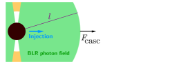
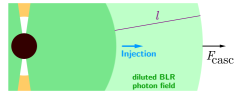
Figure 1:

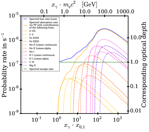
Figure 2: Various channels of the photon loss rate for case 1_a on the left-hand side ordinate vs. the HE photon energy. On the right-hand side ordinate, we show the optical depth corresponding to the respective photon loss rate contribution.

3 Modeling of Inverse-Compton Pair Cascades in the 3C 279 Broad-Line Region

We assume that relativistic pairs or gamma rays are injected into the jet plasma of 3C 279 initiating IC pair cascades on the soft photons of the BLR. The injection of nonthermal energy can result from processes such as diffusive shock acceleration (Summerlin & Baring 2012; Marscher 2014; Baring et al. 2017), stochastic acceleration (Lefa et al. 2011; Asano & Hayashida 2015), magnetoluminescence (Blandford et al. 2017; Matthews et al. 2020), shear acceleration (Rieger & Mannheim 2002; Rieger et al. 2007; Rieger 2019), wakefield acceleration by Alfvén waves excited at the base of the jet (Ebisuzaki & Tajima 2014), or by acceleration in kink-unstable magnetically dominated flows (Appl et al. 2000; Giannios & Spruit 2006), see the review by Blandford et al. (2019). A Gaussian electron distribution can arise from particle acceleration in a sporadically active magnetospheric vacuum gap (Hirotani et al. 2021, and references therein). We note that a proton beam propagating through the central parsec could inject secondaries where in situ acceleration of electrons and positrons to high energies is quenched due to strong energy losses (Lovelace 1976; Mannheim 1993; Mastichiadis & Kirk 1995). We inject PL photons plus Gaussian electrons in cases 1_a, 1_b and 1_c, log-parabolic photons in case 2, and PL plus Gaussian electrons in case 3.

Similar to the approaches by Zdziarski (1988) and Blandford & Levinson (1995), the emerging spectra from this scenario can be numerically computed with a code that solves the coupled kinetic equations for the repeated interactions of relativistic electrons (positrons) and gamma-ray photons with a background field of low-energy photons (Wendel et al. 2021). Three homogeneous, isotropic, and time-independent distributions are included: the distribution of relativistic electrons with Lorentz factor $\gamma\gg 1$ and spectral number density $N(\gamma)$, the distribution of gamma-ray photons with energy $x_{\gamma}\gg 1$ and spectral number density $n_{\gamma}(x_{\gamma})$ and the distribution of low-energy photons with energy $x\ll 1$ and spectral number density $n_{0}(x)$, which is assumed to be a set of broad emission lines in the following. Energies are in units of $m_{\rm e}c^{2}$. Pair production involves collisions of the gamma-ray photons with low-energy photons, destroying the incident photons and supplying new electrons. IC scattering involves collisions of electrons with low-energy photons. The electrons lose energy but remain in the system and can IC scatter again. The gamma-ray photons produced are available for another generation of PP. The spectral IC production rate of gamma-ray photons per unit volume is denoted by $\dot{n}_{\gamma,\,\rm{IC}}(x_{\gamma})$. Allowing injection of gamma-ray photons with spectral rate $\dot{n}_{\gamma,\,\rm i}(x_{\gamma})$ as well as injection of electrons with spectral rate $\dot{N}_{\rm i}(\gamma)$, an IC pair cascade develops through the interplay of PP and IC scattering, affecting the relativistic electrons and the gamma-ray photons, while the soft target photons have a fixed density. For the escape of the electrons and photons from the interaction region, an energy-independent escape time is adopted. Hence, photons disappear through two channels, namely, by pair absorption and by escape. Instead of assuming that the gamma-ray emitting region is located outside of the BLR, we assume that it lies at the edge of the BLR such that the BLR photons act as target photons for the cascade, but do not lead to further pair absorption beyond the emission region.

To study the effect of the many possible acceleration mechanisms on the emerging SED, we assume three different generic injection terms:

Case 1: gamma-ray photons from the inner portion of 3C 279 as well as electrons that have been accelerated to energies around a mean energy $\gamma_{\rm{mean}}$ with spread $\varsigma$ in energy (e.g. from a voltage drop of a presumed magnetospheric vacuum gap) interact with photons from the BLR. Hence, as input to the code we prescribe $\dot{n}_{\gamma,\,\rm i}$ and $\dot{N}_{\rm i}$. For the photon injection, we use a PL

$$\dot{n}_{\gamma,\,\rm i}(x_{\gamma})=\left\{\begin{array}[]{ll}K_{{\rm P}}\left(\frac{x_{\gamma}}{x_{\gamma,\,1}}\right)^{\alpha}&\mathrm{if}\;x_{\gamma,\,1}\leq x_{\gamma}\leq x_{\gamma,\,0}\\ 0&\mathrm{otherwise,}\end{array}\right.$$ (1)

while we model the electron distribution by a Gaussian

$$\dot{N}_{\rm i}(\gamma)=\left\{\begin{array}[]{ll}\frac{K_{\rm{G}}}{\varsigma\sqrt{(}2\pi)}\cdot\exp\left(-\frac{(\gamma-\gamma_{\mathrm{mean}})^{2}}{2\,\varsigma^{2}}\right)&\mathrm{if}\;\gamma_{{\mathrm{i}},\,1}\leq\gamma\leq\gamma_{{\mathrm{i}},\,0}\mathrm{,}\\ 0&\mathrm{otherwise.}\end{array}\right.$$ (2)

Case 2: Only gamma-ray photons interact with BLR photons. One has to specify $\dot{n}_{\gamma,\,\rm i}$, while $\dot{N}_{\rm i}=0$. We restrict the photon spectral injection rate to a log-parabola:

$$\dot{n}_{\gamma,\,\rm i}(x_{\gamma})=\left\{\begin{array}[]{ll}K_{{\rm P}}\left(\frac{x_{\gamma}}{x_{\gamma,\,1}}\right)^{\alpha+\beta\log_{10}(x_{\gamma}/x_{\gamma,\,1})}&\mathrm{if}\;x_{\gamma,\,1}\leq x_{\gamma}\leq x_{\gamma,\,0}\\ 0&\mathrm{otherwise}\end{array}\right.$$ (3)

Case 3: Purely electrons interact with photons from the BLR. Only $\dot{N}_{\rm i}$ has to be defined and $\dot{n}_{\gamma,\,\rm i}=0$. The electron distribution is prescribed by a PL plus Gaussian:

$$\dot{N}_{\rm i}(\gamma)=\left\{\begin{array}[]{ll}K_{{\rm P}}\gamma^{\alpha}+\frac{K_{\rm{G}}}{\varsigma\sqrt{(}2\pi)}\cdot\exp\left(-\frac{(\gamma-\gamma_{\mathrm{mean}})^{2}}{2\,\varsigma^{2}}\right)&\mathrm{if}\;\gamma_{{\mathrm{i}},\,1}\leq\gamma\leq\gamma_{{\mathrm{i}},\,0}\mathrm{,}\\ 0&\mathrm{otherwise}\end{array}\right.$$ (4)

In all cases we choose

$$n_{0}(x)=K_{\rm{lines}}\cdot\sum_{i}\frac{K_{{\rm{line}},\,i}}{x_{0,\,i}}\cdot\delta_{\mathrm{Dirac}}\left(x-x_{0,\,i}\right)$$ (5)

being a sum of Dirac delta distributions situated at mid-UV (MUV) to soft X-ray energies $x_{0,\,i}=h/(\lambda_{0,\,i}\,m_{\rm{e}}\,c)$. This approximates that the background photon field $n_{0}$ is a set of emission lines at the wavelengths $\lambda_{0,\,i}$. Each emission line is defined by its photon energy $x_{0,\,i}$ and by $K_{{\rm{line}},\,i}$, which is its flux density relative to that of the hydrogen Balmer-$\beta$ line. $K_{\rm{lines}}$ is a parameter affecting the total number density of the soft photons. The fact that the cascade evolves with BLR photons as targets reflects that the cascade happens within or at least not far away from the BLR.

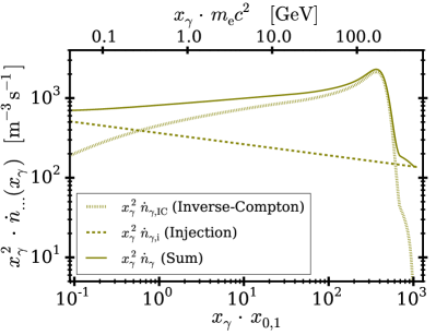
Figure 3: Product of the squared HE photon energy with the spectral production rate of photons (dotted), with the injection rate (dashed), as well as with the sum of both (solid) vs. the product of the HE photon energy with the energy of the highest energetic line (bottom abscissa) and vs. the HE photon energy in GeV (top abscissa).

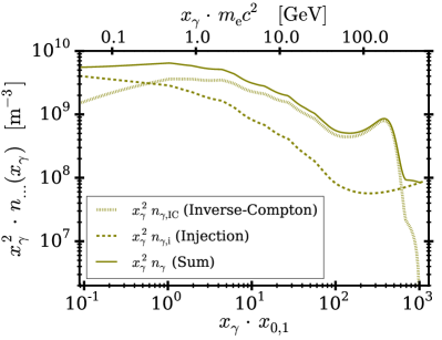
Figure 4: Product of the squared HE photon energy with the spectral number density of photons (solid) as well as with its two contributions $n_{\gamma,\,\mathrm{i}}$ (dashed) and $n_{\gamma,\,\mathrm{IC}}$ (dotted) vs. the product of the HE photon energy with the energy of the highest energetic line (bottom abscissa) and vs. the HE photon energy in GeV (top abscissa).

All curves are for case 1_a. For the exact meaning of the plotted quantities, see section 3 or Wendel et al. (2021).

The escape timescale of both the electrons and the photons is approximated by $T_{\rm{esc}}:=l/c$, where $l$ is the energy-independent escape length (identified with the radius $R$ of the interaction region in Wendel et al. (2021)). As we assume the injection taking place in the interior of the BLR, the quantity $l$ is also equivalent to the radial size of the BLR. Outside of the radial distance $l$, the radiation is assumed to escape without additional absorption due to the $r^{-2}$ dilution of the BLR field, see the discussion in Marcowith et al. (1995) and Vuillaume et al. (2018).

Eventually, from the injection rates, from $n_{0}$, and from $T_{\rm{esc}}$, the code iteratively determines the steady-state $N$. We iterate the values of $N$ as long as the relative change of $N$ between two successive iteration steps is $\geq 0.01$ for $\gamma>10/x_{0,\,1}$ and $\geq 0.01\cdot(\gamma\,x_{0,\,1}/10)^{2}$ for $\gamma\leq 10/x_{0,\,1}$. From $N$, we compute $\dot{n}_{\gamma,\,\rm{IC}}$ and $n_{\gamma}$. We note that as obvious from equation 1 in Wendel et al. (2021), $n_{\gamma}$ is the sum of the two contributions $n_{\gamma,\,\mathrm{i}}$, i.e. the photon injection rate attenuated by the loss rate, and $n_{\gamma,\,\mathrm{IC}}$, i.e. the IC photon production rate attenuated by the loss rate.

As the flux of injected particles might be well collimated, the escaping photons are assumed to leave the interaction region also along a beam of small opening angle $\phi$. After leaving the AGN, we assume propagation without pair absorption due to the infrared torus and extragalactic background light which becomes relevant only at higher energies (MAGIC Collaboration et al. 2008). Then, the detected flux density $F_{\rm{casc}}(x_{\gamma})$ is determined from $n_{\gamma}$ by equation 3 of Wendel et al. (2021). To show that the gamma-ray emission of 3C 279 originates from the BLR, it is sufficient to find the parameters of equations 1 - 5, as well as $l$ and $\phi$, such that $F_{\rm{casc}}$ meets the observed flux density.

4 Results and conclusions

In the cases 1_a, 2, and 3, the observations can be fitted with our theoretical model by choosing appropriate input parameters yielding the acceptable reduced chi-squares $\chi_{\rm{red}}^{2}$ listed in table 4. Conventional least squares fits with log-parabolic or PL with exponential cutoff models yield $\chi_{\rm{red}}^{2}$s of 1.2 or 3.3, respectively. We note that the cutoff parameters $x_{\gamma,\,1}$, $x_{\gamma,\,0}$, $\gamma_{{\rm{i}},\,1}$, and $\gamma_{{\rm{i}},\,0}$ were not obtained by fitting, but were chosen to lie below and above the Fermi sensitivity range.

For the BLR spectrum we choose emission lines from the MUV, far-UV, extreme-UV (EUV), and soft X-ray regime as shown in table 4. We include lines that are prominent in observational BLR spectra and in synthetic spectra. Strong lines which are neighboring in $x$ by less than $\approx 10\,\%$ are treated as one single line. We treat the numbers $K_{{\rm{line}},\,i}$ as parameters free within reasonable borders. We choose $K_{{\rm{line}},\,i}$ such that the tips in the pair-absorption rate (see figure 2) create troughs in the cascaded spectrum so that the observed SED is met.

Table 1: Emission Lines, Used as the Soft Target Photons

$i\,\,$	Line Designation	Wavelength $\lambda_{0,\,i}$			Relative Flux Density Contribution $K_{{\rm{line}},\,i}$
		[$\rm{nm}$]			Case 1a	Case 2	Case 3
1	O VII a, b, c		2.	20	5.90	4.80	5.20
lightgrayblack 2			C V a, b		4.	05	3.55	4.25	3.45
lightgrayblack 3			Fe XVIII b, c		9.	39	4.70	5.75	5.05
lightgrayblack 4			Fe XXIII b, c		13.	3	3.95	2.90	3.80
lightgrayblack 5			He II Lyman continuum a		22.	8	0.75	0.45	0.70
lightgrayblack 6			He II Lyman-$\alpha$ a, b, c		30.	5	3.70	2.90	3.50
lightgrayblack 7			He I a, b, c		58.	4	4.80	4.75	5.30
lightgrayblack 8			H I Lyman continuume		93.	0	1.75	1.60	1.75
lightgrayblack 9			H I Lyman-$\alpha$ a, b, c, d, e		122		4.35	1.70	4.35
lightgrayblack 10			C IV a, b, c, d, e		155		1.85	0.70	1.90
lightgrayblack 11			Mg II b, c, d, e		280		0.55	0.20	0.60

As can be seen in table 4, the $K_{{\rm{line}},\,i}$ in the soft X-ray regime are of similar order of magnitude as the $K_{{\rm{line}},\,i}$ in the UV regime. This is the case because in our approach the numbers $K_{{\rm{line}},\,i}$ are not to be understood as a proxy for the equivalent widths of the lines. Typical BLR spectra consist of emission lines and of continuum emission reflected from the illuminating accretion disk and X-ray-emitting corona (see Tavecchio & Ghisellini 2008). This continuum emission is also included in the coefficients $K_{{\rm{line}},\,i}$.

We show the spectral pair-absorption rate of case 1_a as well as the corresponding optical depth in figure 2. The corresponding plots for cases 2 and 3 look qualitatively similar. The course of our optical depth with energy from $10\,\rm{GeV}$ up to $\approx 90\,\rm{GeV}$ is similar (slightly larger in comparison) to the one of Liu & Bai (2006) with assuming the gamma-ray-emitting region at the inner edge of the BLR (dashed line in their figure 8). Between $\approx 30\,\rm{GeV}$ and $\approx 90\,\rm{GeV}$ our optical depth is similar to the one by the H.E.S.S. Collaboration et al. (2019) with assuming a shell-like BLR and emission from slightly within the BLR (cyan curves in the left-hand panel of their figure 5) or with assuming a ring-like BLR and emission from deeply within the BLR (blue curves in the right-hand panel of their figure 5). In contrast to Liu & Bai (2006) and the H.E.S.S. Collaboration et al. (2019), in our case inclusion of EUV and soft X-ray lines results in extension of the optical depth to energies below $1\,\rm{GeV}$. Above $\approx 90\,\rm{GeV}$, our optical depth decreases with energy due to the neglected NUV and optical lines. Tavecchio & Mazin (2009) and the H.E.S.S. Collaboration et al. (2019) have stronger optical to IR contribution in their target spectra and thus higher optical depths above $\approx 100\,\rm{GeV}$. In comparison to the shell-like BLR model of Tavecchio & Ghisellini (2012) with comparable disk luminosity, our optical depth is higher below $\approx 10\,\rm{GeV}$, but above that it is of the same order of magnitude.

We also show the photon injection rate $\dot{n}_{\gamma,\,\rm i}$, the production rate $\dot{n}_{\gamma,\,\rm{IC}}$ as well as their sum $\dot{n}_{\gamma}$ exemplarily for case 1_a in figure 4. In case 1_a, at energies below $\approx 2\,\rm{GeV}$, the emerging radiation is composed about equally from $\dot{n}_{\gamma,\,\mathrm{i}}$ and from $\dot{n}_{\gamma,\,\mathrm{IC}}$. With increasing energy, the contribution of the injected photons decreases, and that one of the IC up-scattered photons increases. In case 2, IC-produced photons dominate the photon population between $\approx 0.4\,\rm{GeV}$ and $\approx 100\,\rm{GeV}$, while as a consequence of the curvature of the log-parabola the injected photons dominate elsewhere. In case 3, there is no photon injection and consequently the entire photon population is due to cascaded radiation.

The photon number density $n_{\gamma}$ and its two contributions $n_{\gamma,\,\rm i}$ (i.e. injection rate divided by loss rate) and $n_{\gamma,\,\rm{IC}}$ (i.e. production rate divided by loss rate) are shown for case 1_a in figure 4. There, the absorption features by the emission lines are seen as the dips above $\approx 0.5\,\rm{GeV}$. The major dip above $\approx 20\,\rm{GeV}$ is caused in all cases by pair absorption on He II, He I and H I emission line photons.

The resulting energy flux densities in comparison to the observational data are shown in figure 4. The bump in the SEDs above $\approx 100\,\rm{GeV}$ is in cases 1_a and 3 the result of strong electron injection around $\approx 200\,\rm{GeV}$, and in case 2 due to the log-parabolic photon injection. The fact that the modeled flux densities can describe the observational ones in the cases 1_a, 2 and 3 means that HE gamma-ray emission from the edge of the BLR is a robust finding and especially independent of the precise composition of the injected species. Interactions of gamma rays with optical emission line photons of stellar radiation fields can produce absorption troughs lacking, however, the features due to EUV or X-ray lines present in the BLR radiation field (Bednarek & Sitarek 2021).

To estimate the total luminosity of the BLR for case 1_a, we determine the total energy density of the soft photons through $u_{\rm{BLR,\,tot}}=K_{\rm{lines}}\cdot\sum_{i=1}^{11}K_{{\rm{line}},\,i}\cdot m_{\rm e}c^{2}$. From this we get the luminosity $L_{\rm{BLR,\,tot}}=u_{\rm{BLR,\,tot}}\cdot c\cdot 4\pi l^{2}=7.4\times 10^{37}\,\rm{W}$. Analogously, we determine the UV luminosity $L_{\rm{BLR,\,UV}}=K_{\rm{lines}}\cdot\sum_{i=4}^{11}K_{{\rm{line}},\,i}\cdot m_{\rm e}c^{2}\cdot c\cdot 4\pi l^{2}=4.5\times 10^{37}\,\rm{W}$. From this we get an estimate of the BLR radius with help of the empirical relation by Kaspi et al. (2007, equation 3 therein), connecting the time-lag-based C IV radius with the UV luminosity. We obtain $R_{\rm C\,IV}=4.5\times 10^{14}\,\rm m$. Considering the scatter of the normalizations in empirical radius luminosity relations (Ghisellini & Tavecchio 2008; Kilerci Eser et al. 2015), the radii $R_{\rm C\,IV}$ and $l$ can be considered similar. For example, using the canonical $10\,\%$ reprocessing fraction (Ghisellini et al. 2017), the disk luminosity is $L_{\rm{disk,\,tot}}=10\,L_{\rm{BLR,\,tot}}$ and the approximate BLR radius is $2.7\times 10^{15}\,\rm{m}$ (Ghisellini & Tavecchio 2008, equation 4 therein).

Now, we argue that emission from outside of the BLR is hardly realizable within our model and the Fermi SED. Modeling a cascade on the diluted BLR photon field outside of the BLR would correspond to a reduced soft photon density, reflected in a reduced $K_{\rm{lines}}$. Exemplarily, for the injection equation 1 and 2 (case 1 injection) we choose $K_{\rm{lines}}$ being $0.25$ of the value reported in table 4, corresponding to dilution of radiation at a doubled distance. The interaction radius is kept the same as in table 4. This means that the injected particles are injected at the outer edge of the BLR and interact with the diluted photon field. If they were injected inside, they would be reprocessed inside, as happening in cases 1_a, 2, and 3. With this reduced $K_{\rm{lines}}$, we obtain the SED depicted by case 1_b in figure 4 with $\chi_{\rm{red}}^{2}=106$. We run a series of simulations and try to find a new set of parameters to fit the Fermi data again with this reduced $K_{\rm{lines}}$. Without raising the BLR luminosity over reasonable values, we do not achieve a model fit significantly better than the case 1_c in figure 4 with $\chi_{\rm{red}}^{2}=12.8$. The slope below $1\,\rm GeV$ cannot be reconciled with the trough above $\approx 3\,\rm GeV$.

Table 2:
Input Parameters, Used to Fit the SED, and Attained $\chi_{\rm{red}}^{2}$

Quantity	Used Value
0	Case 1a	Case 2	Case 3
$x_{\gamma,\,1}$	$2.0\times 10^{2}$	$2.0\times 10^{2}$	0
lightgrayblack $x_{\gamma,\,0}$	$9.8\times 10^{5}$	$9.8\times 10^{5}$	0
lightgrayblack $\gamma_{{\rm{i}},\,1}$	$\gamma_{\rm{mean}}-3\varsigma$	0	$98$
lightgrayblack $\gamma_{{\rm{i}},\,0}$	$\gamma_{\rm{mean}}+3\varsigma$	0	$9.8\times 10^{5}$
lightgrayblack $\phi\,\,\,[\arcdeg]$	$2.0$	$2.0$	$2.0$
lightgrayblack $l\,\,\,[\rm{m}]$	$2.4\times 10^{15}$	$2.4\times 10^{15}$	$2.4\times 10^{15}$
lightgrayblack $K_{\rm{lines}}\,\,\,[\rm{m^{-3}}]$	$1.2\times 10^{9}$	$1.1\times 10^{9}$	$1.2\times 10^{9}$
lightgrayblack $K_{\rm{G}}\,\,\,[\rm{s^{-1}m^{-3}}]$	$5.8\times 10^{-3}$	0	$6.5\times 10^{-3}$
lightgrayblack $K_{\rm{P}}\,\,\,[\rm{s^{-1}m^{-3}}]$	$0.012$	$0.014$	$8.9\times 10^{3}$
lightgrayblack $\gamma_{\rm{mean}}$	$3.9\times 10^{5}$	0	$3.9\times 10^{5}$
lightgrayblack $\varsigma/\gamma_{\rm{mean}}$	$0.20$	0	$0.20$
lightgrayblack $\alpha$	$-2.1$	$-2.2$	$-2.3$
lightgrayblack $\beta$	0	$0.068$	0
lightgrayblack $\chi_{\rm{red}}^{2}$	$0.90$	$0.62$	$0.83$

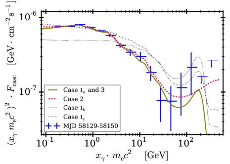
Table 3: Energy flux density vs. HE photon energy for the cases considered as well as for the Fermi LAT observation. Cases 1_a and 3 are indistinguishable within drawing accuracy. The olive solid and the purple dashed curves depict cascades in the BLR field, while the gray dotted and dashed-dotted ones depict cascades on the diluted BLR field.

5 Summary

It is generally accepted that lepto-hadronic emission models can describe the nonthermal SEDs of blazars such as 3C 279 based on the assumption of particle acceleration at shock waves traveling down the jets. The high amplitudes and short timescales of the gamma-ray flux variations, however, indicate the injection of major dissipative events showing temporal and spectral features that call for explanations beyond the shock acceleration scenario (Shukla & Mannheim 2020; Wendel et al. 2021).

Here, we have shown that the gamma-ray spectrum of 3C 279 measured with high precision in an active state is in agreement with an IC pair cascade spectrum initiated by a beam of pairs or gamma rays, including absorption troughs from the interactions of the gamma rays and pairs with emission line photons from the edge of the BLR.

We investigated three possible cases that differ mainly in the functional shape of the injected species. In all three cases we considered the radiation field of the BLR region as a target. The emerging spectra of the cascade were computed numerically and are superpositions of the injected spectra attenuated by pair absorption and of IC up-scattered emission. We achieved fits to the data in all three cases and found the BLR UV-luminosity-based radius being of the same order of magnitude as the radial size of the cascade region.

A cascade taking place outside of the BLR was modeled by choosing a lower density of the soft photon field and the same size of the interaction region (escape timescale). We found, however, that this precludes us from achieving satisfactory fits to the data, strengthening our interpretation of the gamma-ray SED observed with Fermi LAT as evidence for emission from the edge of the BLR.

If a sheath surrounding the jet blocks the BLR photons, the cascade could be initiated by particles accelerated much deeper within the BLR. Moreover, multiple emitting regions could exist simultaneously and could propagate along the jet (Stern & Poutanen 2011; Stern & Poutanen 2014; Aleksić et al. 2014; Lei & Wang 2015; Finke 2016; Rani et al. 2018; Patiño-Álvarez et al. 2019; Shukla & Mannheim 2020; Acharyya et al. 2021). It may therefore be difficult to generalize our conclusions, unless there is a causal connection between the gamma-ray emitting region and the BLR.

References

- Abolmasov & Poutanen (2017) Abolmasov, P., & Poutanen, J. 2017, MNRAS, 464, 152, doi: 10.1093/mnras/stw2326
- Acharyya et al. (2021) Acharyya, A., Chadwick, P. M., & Brown, A. M. 2021, MNRAS, 500, 5297, doi: 10.1093/mnras/staa3483
- Ackermann et al. (2016) Ackermann, M., Anantua, R., Asano, K., et al. 2016, ApJ, 824, L20, doi: 10.3847/2041-8205/824/2/L20
- Aleksić et al. (2014) Aleksić, J., Ansoldi, S., Antonelli, L. A., et al. 2014, A&A, 567, A41, doi: 10.1051/0004-6361/201323036
- Appl et al. (2000) Appl, S., Lery, T., & Baty, H. 2000, A&A, 355, 818. https://ui.adsabs.harvard.edu/abs/2000A&A...355..818A
- Asano & Hayashida (2015) Asano, K., & Hayashida, M. 2015, ApJ, 808, L18, doi: 10.1088/2041-8205/808/1/L18
- Atwood et al. (2009) Atwood, W. B., Abdo, A. A., Ackermann, M., et al. 2009, ApJ, 697, 1071, doi: 10.1088/0004-637X/697/2/1071
- Baring et al. (2017) Baring, M. G., Böttcher, M., & Summerlin, E. J. 2017, MNRAS, 464, 4875, doi: 10.1093/mnras/stw2344
- Bednarek & Sitarek (2021) Bednarek, W., & Sitarek, J. 2021, MNRAS, 503, 2423, doi: 10.1093/mnras/stab554
- Blandford et al. (2019) Blandford, R., Meier, D., & Readhead, A. 2019, ARA&A, 57, 467, doi: 10.1146/annurev-astro-081817-051948
- Blandford et al. (2017) Blandford, R., Yuan, Y., Hoshino, M., & Sironi, L. 2017, Space Sci. Rev., 207, 291, doi: 10.1007/s11214-017-0376-2
- Blandford & Levinson (1995) Blandford, R. D., & Levinson, A. 1995, ApJ, 441, 79, doi: 10.1086/175338
- Böttcher & Els (2016) Böttcher, M., & Els, P. 2016, ApJ, 821, 102, doi: 10.3847/0004-637X/821/2/102
- Britto et al. (2015) Britto, R. J. G., Razzaque, S., & Lott, B. 2015, arXiv e-prints, arXiv:1502.07624. https://arxiv.org/abs/1502.07624
- Cash (1979) Cash, W. 1979, ApJ, 228, 939, doi: 10.1086/156922
- Dere et al. (1997) Dere, K. P., Landi, E., Mason, H. E., Monsignori Fossi, B. C., & Young, P. R. 1997, A&AS, 125, 149, doi: 10.1051/aas:1997368
- Dermer et al. (2014) Dermer, C. D., Cerruti, M., Lott, B., Boisson, C., & Zech, A. 2014, ApJ, 782, 82, doi: 10.1088/0004-637X/782/2/82
- Donea & Protheroe (2003) Donea, A.-C., & Protheroe, R. J. 2003, Astroparticle Physics, 18, 377, doi: 10.1016/S0927-6505(02)00155-X
- Ebisuzaki & Tajima (2014) Ebisuzaki, T., & Tajima, T. 2014, Astroparticle Physics, 56, 9, doi: 10.1016/j.astropartphys.2014.02.004
- Finke (2016) Finke, J. D. 2016, ApJ, 830, 94, doi: 10.3847/0004-637X/830/2/94
- Ghisellini et al. (2017) Ghisellini, G., Righi, C., Costamante, L., & Tavecchio, F. 2017, MNRAS, 469, 255, doi: 10.1093/mnras/stx806
- Ghisellini & Tavecchio (2008) Ghisellini, G., & Tavecchio, F. 2008, MNRAS, 387, 1669, doi: 10.1111/j.1365-2966.2008.13360.x
- Giannios & Spruit (2006) Giannios, D., & Spruit, H. C. 2006, A&A, 450, 887, doi: 10.1051/0004-6361:20054107
- Hartman et al. (1992) Hartman, R. C., Bertsch, D. L., Fichtel, C. E., et al. 1992, ApJ, 385, L1, doi: 10.1086/186263
- Hayashida et al. (2015) Hayashida, M., Nalewajko, K., Madejski, G. M., et al. 2015, ApJ, 807, 79, doi: 10.1088/0004-637X/807/1/79
- H.E.S.S. Collaboration et al. (2019) H.E.S.S. Collaboration, Abdalla, H., Adam, R., et al. 2019, A&A, 627, A159, doi: 10.1051/0004-6361/201935704
- Hirotani et al. (2021) Hirotani, K., Krasnopolsky, R., Shang, H., Nishikawa, K.-i., & Watson, M. 2021, ApJ, 908, 88, doi: 10.3847/1538-4357/abd3a6
- Hunter (2007) Hunter, J. D. 2007, Computing in Science and Engineering, 9, 90, doi: 10.1109/MCSE.2007.55
- Kaspi et al. (2007) Kaspi, S., Brandt, W. N., Maoz, D., et al. 2007, ApJ, 659, 997, doi: 10.1086/512094
- Kilerci Eser et al. (2015) Kilerci Eser, E., Vestergaard, M., Peterson, B. M., Denney, K. D., & Bentz, M. C. 2015, ApJ, 801, 8, doi: 10.1088/0004-637X/801/1/8
- Kim et al. (2020) Kim, J.-Y., Krichbaum, T. P., Broderick, A. E., et al. 2020, A&A, 640, A69, doi: 10.1051/0004-6361/202037493
- Landi et al. (2012) Landi, E., Del Zanna, G., Young, P. R., Dere, K. P., & Mason, H. E. 2012, ApJ, 744, 99, doi: 10.1088/0004-637X/744/2/99
- Lefa et al. (2011) Lefa, E., Rieger, F. M., & Aharonian, F. 2011, ApJ, 740, 64, doi: 10.1088/0004-637X/740/2/64
- Lei & Wang (2015) Lei, M., & Wang, J. 2015, PASJ, 67, 79, doi: 10.1093/pasj/psv055
- Liu & Bai (2006) Liu, H. T., & Bai, J. M. 2006, ApJ, 653, 1089, doi: 10.1086/509097
- Lovelace (1976) Lovelace, R. V. E. 1976, Nature, 262, 649, doi: 10.1038/262649a0
- MAGIC Collaboration et al. (2008) MAGIC Collaboration, Albert, J., Aliu, E., et al. 2008, Science, 320, 1752, doi: 10.1126/science.1157087
- Mannheim (1993) Mannheim, K. 1993, A&A, 269, 67. https://arxiv.org/abs/astro-ph/9302006
- Marcowith et al. (1995) Marcowith, A., Henri, G., & Pelletier, G. 1995, MNRAS, 277, 681, doi: 10.1093/mnras/277.2.681
- Marscher (2014) Marscher, A. P. 2014, ApJ, 780, 87, doi: 10.1088/0004-637X/780/1/87
- Marziani et al. (1996) Marziani, P., Sulentic, J. W., Dultzin-Hacyan, D., Calvani, M., & Moles, M. 1996, ApJS, 104, 37, doi: 10.1086/192291
- Mastichiadis & Kirk (1995) Mastichiadis, A., & Kirk, J. G. 1995, A&A, 295, 613. https://ui.adsabs.harvard.edu/abs/1995A&A...295..613M
- Matthews et al. (2020) Matthews, J. H., Bell, A. R., & Blundell, K. M. 2020, New A Rev., 89, 101543, doi: 10.1016/j.newar.2020.101543
- Mattox et al. (1996) Mattox, J. R., Bertsch, D. L., Chiang, J., et al. 1996, ApJ, 461, 396, doi: 10.1086/177068
- Meyer et al. (2021) Meyer, M., Petropoulou, M., & Christie, I. M. 2021, ApJ, 912, 40, doi: 10.3847/1538-4357/abedab
- Meyer et al. (2019) Meyer, M., Scargle, J. D., & Blandford, R. D. 2019, ApJ, 877, 39, doi: 10.3847/1538-4357/ab1651
- Oliphant (2015) Oliphant, T. E. 2015, Guide to NumPy, 2nd edn. (North Charleston, SC, USA: CreateSpace Independent Publishing Platform)
- Patiño-Álvarez et al. (2019) Patiño-Álvarez, V. M., Dzib, S. A., Lobanov, A., & Chavushyan, V. 2019, A&A, 630, A56, doi: 10.1051/0004-6361/201834401
- Pian et al. (2005) Pian, E., Falomo, R., & Treves, A. 2005, MNRAS, 361, 919, doi: 10.1111/j.1365-2966.2005.09216.x
- Pittori et al. (2018) Pittori, C., Lucarelli, F., Verrecchia, F., et al. 2018, ApJ, 856, 99, doi: 10.3847/1538-4357/aab1f9
- Poutanen & Stern (2010) Poutanen, J., & Stern, B. 2010, ApJ, 717, L118, doi: 10.1088/2041-8205/717/2/L118
- Rani et al. (2018) Rani, B., Jorstad, S. G., Marscher, A. P., et al. 2018, ApJ, 858, 80, doi: 10.3847/1538-4357/aab785
- Reimer (2007) Reimer, A. 2007, ApJ, 665, 1023, doi: 10.1086/519766
- Rieger (2019) Rieger, F. M. 2019, Galaxies, 7, 78, doi: 10.3390/galaxies7030078
- Rieger et al. (2007) Rieger, F. M., Bosch-Ramon, V., & Duffy, P. 2007, Ap&SS, 309, 119, doi: 10.1007/s10509-007-9466-z
- Rieger & Mannheim (2002) Rieger, F. M., & Mannheim, K. 2002, A&A, 396, 833, doi: 10.1051/0004-6361:20021457
- Shah et al. (2019) Shah, Z., Jithesh, V., Sahayanathan, S., Misra, R., & Iqbal, N. 2019, MNRAS, 484, 3168, doi: 10.1093/mnras/stz151
- Shukla & Mannheim (2020) Shukla, A., & Mannheim, K. 2020, Nature Communications, 11, 4176, doi: 10.1038/s41467-020-17912-z
- Stern & Poutanen (2011) Stern, B. E., & Poutanen, J. 2011, MNRAS, 417, L11, doi: 10.1111/j.1745-3933.2011.01107.x
- Stern & Poutanen (2014) —. 2014, ApJ, 794, 8, doi: 10.1088/0004-637X/794/1/8
- Summerlin & Baring (2012) Summerlin, E. J., & Baring, M. G. 2012, ApJ, 745, 63, doi: 10.1088/0004-637X/745/1/63
- Tan et al. (2020) Tan, C., Xue, R., Du, L.-M., et al. 2020, ApJS, 248, 27, doi: 10.3847/1538-4365/ab8cc6
- Tavecchio & Ghisellini (2008) Tavecchio, F., & Ghisellini, G. 2008, MNRAS, 386, 945, doi: 10.1111/j.1365-2966.2008.13072.x
- Tavecchio & Ghisellini (2012) —. 2012, arXiv e-prints, arXiv:1209.2291. https://arxiv.org/abs/1209.2291
- Tavecchio & Mazin (2009) Tavecchio, F., & Mazin, D. 2009, MNRAS, 392, L40, doi: 10.1111/j.1745-3933.2008.00584.x
- Telfer et al. (2002) Telfer, R. C., Zheng, W., Kriss, G. A., & Davidsen, A. F. 2002, ApJ, 565, 773, doi: 10.1086/324689
- Vuillaume et al. (2018) Vuillaume, T., Henri, G., & Petrucci, P. O. 2018, A&A, 620, A41, doi: 10.1051/0004-6361/201731899
- Wendel et al. (2021) Wendel, C., Becerra González, J., Paneque, D., & Mannheim, K. 2021, A&A, 646, A115, doi: 10.1051/0004-6361/202038343
- Zdziarski (1988) Zdziarski, A. A. 1988, ApJ, 335, 786, doi: 10.1086/166967