Swanson Hamiltonian: non-PT-symmetry phase.

Abstract

In this work, we study the non-hermitian Swanson hamiltonian, particularly the non-PT symmetry phase. We use the formalism of Gel’fand triplet to construct the generalized eigenfunctions and the corresponding spectrum. Depending on the region of the parameter model space, we show that the Swanson hamiltonian represents different physical systems, i.e. parabolic barrier, negative mass oscillators. We also discussed the presence of Exceptional Points of infinite order.

keywords: PT-symmetry Swanson Hamiltonian, Gel’fand triplet, Exceptional Points.

I Introduction.

The study of non-hermitian Parity-Time Reversal(PT) symmetry hamiltonians was proposed in the pioneering work of Bender and Boettcher bender0 . A parametric family of hamiltonians can be obtained by varying the different variables of the corresponding systems. The essential feature of a PT-symmetric Hamiltonian is the existence of certain values of the parameters at which the spectrum is real and the hamiltonian is similar to a hermitian one bender1 ; bender2 ; bender3 ; bender4 ; bender5 ; bender6 . For other values of the parameters of the model, the spectrum contains complex-conjugate pairs of eigenvalues and the corresponding eigenfunctions are non longer PT-symmetric. In the boundary of both regions of the model space, two or more eigenvalues and their corresponding eigenstates can be coalescent, these set of parameters are called Exceptional Points ep1 ; ep2 ; ep3 ; ep4 ; ep5 ; ep6 ; ep7 ; ep8 ; ep9 ; ep10 ; znojil-pe1 ; znojil-pe2 ; znojil-pe3 . The time evolution of a given initial state under the action of these hamiltonians strongly depends on the characteristics of the spectrum, particular at EPs garmon1 ; garmon2 ; garmon3 ; garmon4 ; hatano1 ; hatano2 ; hatano3 ; hatano4 ; nos1 ; nos2 , where the exponential law is generally not valid.

The Swanson model has been introduced in swanson as an example of a hamiltonian that obeys PT-symmetry. It admits real eigenvalues for a well-defined region of the parameter model space. The similarity between the Swanson hamiltonian and the harmonic oscillator as well as the dynamic of observables in the PT-symmetry region have been extensively analyzed ahmed1 ; ahmed2 ; geyer ; quense ; sinha-sw1 ; sinha-sw2 ; sinha-sw3 ; sw-1 ; sw-2 ; fring-sw ; sw-close1 ; mostaf-sw ; mostaf-general ; znojil-sw-inner ; fring . Among the extensions of the Swanson model we can include super-symmetry realizations sinha-sw-susy ; sw-susy . Also, the Swanson hamiltonian has been studied as a particular case of different non-hermitian generalizations of anharmonic oscillators systems znojil-osc1 ; znojil-osc-exp ; znojil-anarm-osc ; znojil-osc2 . Another approach to the Swanson model comes from investigating different q-deformation boson algebras fring-sw3 ; fring-sw1 ; fring-sw2 ; nos3 . As an example, in fring-sw3 different representations of deformed canonical variables fring-sw3 are presented. In this work, the effect that produces the modification of the generalized canonical variables commutator, over the region of PT-symmetry and exceptional points, is analyzed. In fring-sw1 , the authors studied the particular case of the Swanson hamiltonian using the generalization of the Milne quantization. In fring-sw2 the Swanson hamiltonian is discussed in the framework the formalism of generalized pseudo bosons. The authors of fring-sw2 , by employing generalized Bogoliubov transformation, present a mapping of the Swanson model to a standard bosons hamiltonian. In nos3 the Swanson model is obtained as the quadratic limit of a deformed general hamiltonian constructed from a non-standard oscillator algebra.

However, to our knowledge, much less has been investigated in the region of PT-broken symmetry. In this line, the authors of sinha-continuum have proposed different generalizations of the Swanson model. They have described the continuum spectrum of the different generalizations by analyzing the corresponding similar hermitian hamiltonians. More recently, the authors of fring-sw4 have studied the solutions of the time-dependent Swanson hamiltonian. By applying the formalism presented in fring-sw6 , their work includes the construction of a time-dependent metric to compute the time evolution of the observables of the system. A new proposal has been presented in fring-sw5 , where the authors construct time-dependent metrics by point transformations. In this work, the construction of non-Hermitian invariants for the Swanson model and the implementation of Dyson maps is analyzed. From another point of view, the authors of mihail-darboux have made use of the Darboux transformation to provide solutions of the Swanson model for a particular set of parameters.

In this work, we study the non-hermitian Swanson hamiltonian, particularly the non-PT symmetry phase. The work is organized as follows. In Section II we analyse the different model space regions. In Subsection II.1 we discuss the use of the formalism of Rigged Hilbert Space to construct the generalized eigenfunctions and the corresponding spectrum of the model. In Subsection II.2 we present our results for each region of the model parameter space. In Section III we formalize the calculation of mean values of observables and their time evolution. Conclusions are drawn in Section IV.

II Formalism.

Let us start with the hamiltonian of the squeezed harmonic oscillator sho ; sho2 ; sho3 . It is given by

$$H=\hbar\omega~{}\left(a^{\dagger}a+\frac{1}{2}\right)+\hbar\alpha~{}({a}^{2}+~{}{a^{\dagger}}^{2}).$$ (1)

As it is well-known sho ; sho2 ; sho3 , its relevance is related to the study of the Heisenberg Uncertainty Relations for the momentum and position operators. The eigenvalues and eigenfunctions of the hamiltonian of Eq.(1), for $|\alpha|<|\omega|/2$, can be obtained analytically, and the lowest eigenstate is a squeezed state, that is a state which minimizes the variance of the momentum operator $\hat{p}$ by increasing the variance of the coordinate operator $\hat{x}$, or vice versa.

Let us consider the Hamiltonian proposed in swanson , which is a non-hermitian generalization of the hamiltonian of Eq.(1). It reads

$$H(\omega,\alpha,\beta)=\hbar\omega~{}\left(a^{\dagger}a+\frac{1}{2}\right)+\hbar\alpha~{}{a}^{2}+\hbar\beta~{}{a^{\dagger}}^{2}.$$ (2)

We can write $a$ and $a^{\dagger}$ in terms of the coordinate operator, ${\hat{x}}$, and of the momentum operator, ${\hat{p}}:$

$$a = \frac{1}{\sqrt{2}}\left(\frac{\hat{x}}{b_{0}}+{\bf i}\frac{b_{0}}{\hbar}\hat{p}\right),$$

$$a^{\dagger} = \frac{1}{\sqrt{2}}\left(\frac{\hat{x}}{b_{0}}-{\bf i}\frac{b_{0}}{\hbar}\hat{p}\right),$$

with $b_{0}$ the characteristic length of the system. The hamiltonian of (2) reads

$$H(\omega,\alpha,\beta) = \frac{1}{2}\hbar(\omega+\alpha+\beta)\left(\frac{\hat{x}}{b_{0}}\right)^{2}$$ (4)

$$+\frac{1}{2}\hbar(\omega-\alpha-\beta)\left(\frac{b_{0}~{}\hat{p}}{\hbar}\right)^{2}$$

$$+\hbar\frac{(\alpha-\beta)}{2}\left(2~{}\hat{x}\frac{{\bf i}}{\hbar}\hat{p}+1\right).$$

It is straightforward to verify that the hamiltonian of Eq.(4) obeys PT-symmetry.

In the other hand, the hermitian conjugate operator, $H_{c}$, is given by $H_{c}(\omega,\alpha,\beta)=H(\omega,\beta,\alpha)$.

Let us introduce, for $\omega\neq\alpha+\beta$, a new set of complementary operators $\hat{P}$ and $\hat{X}$ , namely:

$$\hat{P} = \left({\hat{p}}+{\bf i}\hbar\frac{\alpha-\beta}{(\omega-\alpha-\beta)b_{0}^{2}}{\hat{x}}\right),$$

$$\hat{X} = {\hat{x}},$$ (5)

$\hat{P}$ and $\hat{X}$ obey the usual commutation relation $[\hat{X},\hat{P}]=\nolinebreak{\bf i}\hbar.$

In terms of ${\hat{P}}$ and $\hat{X}$ the Hamiltonian of Eq.(4) can be written as

$$H=\frac{1}{2m}~{}\hat{P}^{2}\phi(X)+\frac{k}{2}~{}{\hat{X}}^{2}\phi(X),$$ (6)

with $k=m~{}\Omega^{2}$ and

$$\Omega=\Omega(\omega,\alpha,\beta) = \sqrt{\omega^{2}-4\alpha\beta}=|\Omega|{\rm{e}}^{{\bf i}\phi},$$ (7)

$$m=m(\omega,\alpha,\beta,b_{0}) = \frac{\hbar}{(\omega-\alpha-\beta)b_{0}^{2}}.$$ (8)

The spectrum and the eigenfunctions of $H$ depend on the sign of the functions $m(\omega,\alpha,\beta,b_{0})$, $\Omega(\omega,\alpha,\beta)^{2}$.

In Figures 1 and 2 we show the behaviour of $\Omega^{2}$ and $m$, as a function of $\alpha/\omega$ and $\beta/\omega$, respectively. It can be observed that $\Omega^{2}$ is a continuous function, while $m$ has a discontinuity at the plane $\alpha/\omega+\beta/\omega-1=0$.

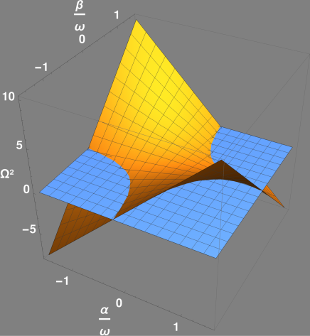
Figure 1: $\Omega^{2}(\omega,\alpha,\beta,b_{0})$ of Eq.(7).

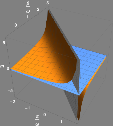
Figure 2: $m(\omega,\alpha,\beta,b_{0})$ of Eq.(8).

There are four possible regions in the parameter model space. If $m>0$ and $\Omega^{2}>0$ the hamiltonian is similar to the usual harmonic oscillator, Region I. The case $m>0$ and $\Omega^{2}<0$ corresponds to a parabolic barrier, Region IIchu1 ; chu2 ; maru ; bermudez . While the case $m<0$ and $\Omega^{2}>0$ can be interpreted as a harmonic oscillator with negative mass, Region III neg-mass-1 ; neg-mass-2 ; neg-mass-3 ; neg-mass-4 ; neg-mass-5 . Finally, the case $m<0$ and $\Omega^{2}<0$ can be interpreted as a parabolic barrier for a system with negative mass, Region IV. The case $k(\omega,\alpha,\beta,b_{0})=0$ corresponds to a free particle. The different regions are displayed in Figure 3 in terms of the adimensional coupling constants $\alpha/\omega$ and $\beta/\omega$.

Figure 3: Different regions of the parameter space in terms of the sign of $m(\omega,\alpha,\beta,b_{0})$ and $\Omega^{2}(\omega,\alpha,\beta,b_{0})$.

II.1 Gelf’and Triplet.

In general, neither $H$ nor $H_{c}$ have eigenfunctions in the Hilbert space ${\cal H}$. To overcome this problem, and to be able to compute the mean value of observables, we shall use the Gel’fand triplet gelfand ; bhom . Let us briefly review the essentials of the formalism.

To describe a quantum system we need a Hausdorff vector space with a convex topology and a scalar product, $(\Psi,\tau)$. The Hilbert space with the topology $\tau_{H}$, $({\mathcal{H}},\tau_{H})$, is the completion of $(\Psi,\tau_{d})$. Let us define another completion of $(\Psi,\tau_{d})$, with a finner topology $\tau_{\Phi}$, $(\Phi,\tau_{\Phi})$, so that $\Phi\subset{\mathcal{H}}\Rightarrow{\mathcal{H}}^{*}\subset\Phi^{*}$. Here, $\Phi^{*}$ is the dual space of $\Phi$, $\Phi^{*}=\{F|F:\Phi\rightarrow{\mathbb{C}},F(v)=\langle F|v\rangle,~{}v\in\Phi\}$. Also, we shall introduce the antidual space of $\Phi$, $\Phi^{\times}$, that is the space of the antilineal functionals on $\Phi$, $\Phi^{\times}=\{G|G:\Phi\rightarrow{\mathbb{C}},G(v)=\langle v|G\rangle,~{}v\in\Phi\}$. Along this lines, we obtain the Gel’fand triplet

$$\Phi\subset{\cal H}\subset\Phi^{\times}.$$ (9)

The extension of the hamiltonian operators $H$ and $H_{c}$ on ${\cal H}$ are the hamiltonian operators $H^{\times}$ and ${H_{c}}^{\times}$ on $\Phi^{\times}$, respectivelely. The eigenfunctions of $H^{\times}$ and ${H_{c}}^{\times}$ are functionals of $\Phi^{\times}$.

In $\Phi^{\times}$, the stationary Schrödinger equation for $H$ and $H_{c}$ can be written as

$$H^{\times}~{}{\widetilde{\phi}}(x)=E~{}{\widetilde{\phi}}(x),$$ (10)

and

$$H_{c}^{\times}~{}{\overline{\psi}}(x)=E_{c}~{}{\overline{\psi}}(x).$$ (11)

For $\omega-\alpha-\beta\neq 0$ we shall introduce the similarity transformation:

$$\Upsilon={\rm{e}}^{-\frac{\alpha-\beta}{\omega-\alpha-\beta}\frac{x^{2}}{2b_{0}^{2}}},$$ (12)

so that

$$\Upsilon~{}H^{\times}~{}\Upsilon^{-1} = h^{\times},$$

$$\Upsilon^{-1}~{}H_{c}^{\times}~{}\Upsilon = h^{\times},$$ (13)

with

$$h^{\times}\phi(x)=-\frac{\hbar^{2}}{2m}\frac{{\rm d}^{2}\phi(x)}{{\rm d}x^{2}}+\frac{1}{2}kx^{2}\phi(x)=E~{}\phi(x),$$ (14)

the eigenfunctions of $H^{\times}$ and $H^{\times}_{c}$ are given by ${\widetilde{\phi}}(x)=\Upsilon^{-1}\phi(x)$ and ${\overline{\psi}}(x)=\Upsilon\phi(x)$, respectively.

Eq. (14) can be interpreted as the Schrödinger equations corresponding to a potential of the form

$$u(x)=\frac{1}{2}kx^{2}=\frac{1}{2}m\Omega^{2}x^{2}.$$ (15)

From Eq.(49), it can be conclude that there is a similarity relation between $H^{\times}$ and $H^{\times}_{c}$, namely $UH^{\times}=H^{\times}_{c}U$, with $U=\Upsilon^{2}$.

As $H^{\times}$ is pseudo-hermitian, we can introduce a new inner product, $\langle.|.\rangle_{U}$, in terms of the positive define operator $U$

$$\langle.|.\rangle_{U}:H^{\times}\times H^{\times}\rightarrow\mathbb{C},~{}\langle{\widetilde{\phi}}_{\nu}|{\widetilde{\phi}}_{\nu^{\prime}}\rangle_{U}=\langle{\widetilde{\phi}}_{\nu}U|{\widetilde{\phi}}_{\nu^{\prime}}\rangle_{.}$$ (16)

It can be observed that the set $\{{\overline{\psi}}_{\nu}\rangle,|{\widetilde{\phi}}_{\nu}\rangle\}$ is bi-orthogonal:

$$\langle{\widetilde{\phi}}_{\nu}|{\widetilde{\phi}}_{\nu^{\prime}}\rangle_{U} = \langle{\overline{\psi}}_{\nu}|{\widetilde{\phi}}_{\nu^{\prime}}\rangle=\langle\phi_{\nu}|\phi_{\nu^{\prime}}\rangle=\delta_{\nu{\nu^{\prime}}}.$$ (17)

The identity operator can be written as

$$\mathds{1}=\sum_{\nu}|{\widetilde{\phi}}_{\nu}\rangle\langle{\overline{\psi}}_{\nu}|.$$ (18)

Given a pseudo-hermitian operator $\hat{Q}$, $\hat{Q}=\Upsilon q\Upsilon^{-1}$ with $q^{\dagger}=q$, its mean value can be computed as

$$\langle{\widetilde{\phi}}|\hat{Q}|{\widetilde{\phi}}\rangle_{U} = \langle{\widetilde{\phi}}|U\hat{Q}|{\widetilde{\phi}}\rangle.$$ (19)

Thus, associated with the operators $p$ and $x$, we have

$$\hat{P} = \Upsilon p\Upsilon^{-1}={\hat{p}}+{\bf i}\hbar\frac{\alpha-\beta}{(\omega-\alpha-\beta)b_{0}^{2}}{\hat{x}},$$

$$\hat{X} = \Upsilon x\Upsilon^{-1}=x,$$ (20)

which is consistent with Eq.(5).

In what follows, we shall present the generalized eigenfunctions and the corresponding spectrum in the different regions.

II.2 Spectrum and Generalized Eigenfunctions.

II.2.1 Region I.

In the PT-symmetry phase, Eq. (14) reduces to the usual harmonic oscillator. Consequently, the spectrum and the eigenfunctions are given by

$$E_{n}=E_{cn} = \hbar\sqrt{\omega^{2}-4\alpha\beta}~{}\left(n+\frac{1}{2}\right),$$

$$\widetilde{\phi}_{n}(x) = {\rm e^{\frac{\alpha-\beta}{\omega-\alpha-\beta}\frac{x^{2}}{2b_{0}^{2}}}}\frac{2^{-\frac{n}{2}}}{\sqrt{\pi}n!}\frac{\sigma}{b_{0}}~{}{\rm e}^{-\frac{x^{2}}{2b^{2}_{0}}\sigma^{2}}~{}H_{n}\left(\frac{x}{b_{0}}\sigma\right),$$

$$\overline{\psi}_{n}(x) = {\rm e^{-\frac{\alpha-\beta}{\omega-\alpha-\beta}\frac{x^{2}}{2b_{0}^{2}}}}\frac{2^{-\frac{n}{2}}}{\sqrt{\pi}n!}\frac{\sigma}{b_{0}}~{}{\rm e}^{-\frac{x^{2}}{2b^{2}_{0}}\sigma^{2}}~{}H_{n}\left(\frac{x}{b_{0}}\sigma\right),$$

with $\sigma=\sqrt{\frac{m\Omega}{\hbar}}b_{0}$ and $\Omega=\sqrt{\omega^{2}-4\alpha\beta}$.

In terms of the eigenfunctions of $H^{\times}$ and ${H_{c}}^{\times}$, the bi-orthogonality relation is given by

$$\int_{-\infty}^{\infty}{\overline{\psi}_{m}^{*}(x)}\widetilde{\phi}_{n}(x)\ dx=\delta_{nm}.$$ (22)

and the completeness relation is

$$\sum_{n}^{\infty}\overline{\psi}^{*}_{n}(x)\widetilde{\phi}_{m}(x^{\prime})=\delta(x-x^{\prime}).$$ (23)

II.2.2 Region III.

In this region, the parameter $m$ takes negative values. As it is proved in Appendix A, we can define $\sigma=\sqrt{\frac{|m\Omega|}{\hbar}}b_{0}\in\mathbb{R}$, as in the previous case. So that

$$E_{n}=E_{cn} = -\hbar\sqrt{\omega^{2}-4\alpha\beta}~{}\left(n+\frac{1}{2}\right),$$

$$\widetilde{\phi}_{n}(x) = \tfrac{2^{-\frac{n}{2}}}{\sqrt{\pi}n!}\tfrac{\sigma}{b_{0}}~{}{\rm e^{\frac{\alpha-\beta}{\omega-\alpha-\beta}\frac{x^{2}}{2b_{0}^{2}}}}{\rm e}^{-\frac{x^{2}}{2b^{2}_{0}}\sigma^{2}}~{}H_{n}\left(\frac{x}{b_{0}}\sigma\right),$$

$$\overline{\psi}_{n}(x) = \tfrac{2^{-\frac{n}{2}}}{\sqrt{\pi}n!}\tfrac{\sigma}{b_{0}}~{}{\rm e^{-\frac{\alpha-\beta}{\omega-\alpha-\beta}\frac{x^{2}}{2b_{0}^{2}}}}{\rm e}^{-\frac{x^{2}}{2b^{2}_{0}}\sigma^{2}}~{}H_{n}\left(\frac{x}{b_{0}}\sigma\right).$$

The bi-orthogonality and completeness relation is the same as in the previous case.

II.2.3 Region II.

In this region, $m>0$ and $\Omega^{2}<0$. The potential $u(x)$ of Eq.(15) corresponds to that of a parabolic barrier chu1 ; chu2 ; maru ; bermudez . Both hamiltonians, $H^{\times}$ and $H_{c}^{\times}$, display continuous spectrum as well as resonant and anti-resonant discrete states.

In Appendix A we present the construction of generalized eigenfunctions and the corresponding eigenvalues. Let us summarize the results as follows.

The generalized eingenfunctions of $H^{\times}$, $\widetilde{\phi}_{n}^{\pm}(x)$, with eigenvalues $E_{n}^{\pm}=\pm{\bf i}\hbar|\Omega|\left(n+\frac{1}{2}\right)$ are given by

$$\widetilde{\phi}_{n}^{\pm}(x) = {\rm e^{\frac{\alpha-\beta}{\omega-\alpha-\beta}\frac{x^{2}}{2b_{0}^{2}}}}\phi_{n}^{\pm}\left(x\right),$$ (25)

while, the generalized eigenfunctions of $H_{c}^{\times}$, $\overline{\psi}_{n}^{\pm}(x)$, with eigenvalues $E_{cn}^{\pm}=\mp{\bf i}\hbar|\Omega|\left(n+\frac{1}{2}\right)$ are given by

$$\overline{\psi}_{n}^{\pm}(x) = {\rm e^{-\frac{\alpha-\beta}{\omega-\alpha-\beta}\frac{x^{2}}{2b_{0}^{2}}}}\phi_{n}^{\mp}\left(x\right).$$ (26)

and

$$\phi_{n}^{-}(x) = \sqrt{\tfrac{\sqrt{i}\sigma}{b_{0}}\frac{1}{2^{n}n!}}{\rm{e}}^{-{\bf i}\sigma^{2}\frac{x^{2}}{2b_{0}^{2}}}H_{n}\left(\frac{\sqrt{{\bf i}}\sigma}{b_{0}}x\right),$$

$$\phi_{n}^{+}(x) = {\phi_{n}^{-}(x)}^{*},$$ (27)

with $\sigma=\sqrt{\frac{|m\Omega|}{\hbar}}b_{0}$.

The bi-orthogonality relation reads

$$\int_{-\infty}^{\infty}(\overline{\psi}_{m}^{\pm}(x))^{*}\widetilde{\phi}_{n}^{\pm}(x)=\delta_{nm},$$ (28)

and the completeness relation is given by

$$\sum_{\begin{array}[]{l}n=0\\ s=\pm\end{array}}^{\infty}~{}(\overline{\psi}_{n}^{s}(x))^{*}\widetilde{\phi}_{n}^{s}(x^{\prime}) = \delta(x-x^{\prime}).$$ (31)

The generalized eigenfunctions associated to the continuous spectrum, $E\in(-\infty,+\infty)$, are given by

$$\widetilde{\phi}_{\pm}^{E}(x) = {\rm e^{\frac{\alpha-\beta}{\omega-\alpha-\beta}\frac{x^{2}}{2b_{0}^{2}}}}~{}\phi_{\pm}^{E}(x),$$ (32)

$$\overline{\psi}_{\pm}^{E}(x) = {\rm e^{-\frac{\alpha-\beta}{\omega-\alpha-\beta}\frac{x^{2}}{2b_{0}^{2}}}}~{}\phi_{\mp}^{E}(x),$$ (33)

with $\nu=-{\bf i}\frac{E}{\hbar|\Omega|}-\frac{1}{2}$ and

$$\phi_{\pm}^{E}(x) = \mathcal{C}~{}\Gamma(\nu+1)D_{-\nu-1}\left(\mp\sqrt{2{\bf i}}\sigma\frac{x}{b_{0}}\right).$$ (34)

The bi-orthogonality and the completeness relation can be written as

$$\int_{-\infty}^{\infty}~{}(\overline{\psi}_{\pm}^{E}(x))^{*}\widetilde{\phi}_{\pm}^{E^{\prime}}(x){\rm dx}=\delta(E-E^{\prime}),$$

$$\sum_{s=\pm}\int_{-\infty}^{\infty}~{}(\overline{\psi}_{s}^{E}(x))^{*}\widetilde{\phi}_{s}^{E}(x){\rm dE}=\delta(x-x^{\prime}).$$

To complete the analysis of this region we have to discuss the analytical properties of the previous solutions.

It is easy to see that the poles of $\phi_{\pm}^{E}(x)$ are those of $\Gamma(\nu+1)$, that is: $-n=\nu+1$, with $n\in\mathbb{N}$ and $E_{n}={\bf i}\hbar|\Omega|\left(n+\frac{1}{2}\right)$.

In the other hand, the poles of $(\phi_{\pm}^{E}(x))^{*}$ are those of $\Gamma(-\nu)$, that is: $n=\nu$, with $n\in\mathbb{N}$ and $E_{n}=-{\bf i}\hbar|\Omega|\left(n+\frac{1}{2}\right)$. As shown in Appendix A, we shall introduce $\eta^{E}_{\pm}(x)=(\phi_{\pm}^{E}(x))^{*}$, which are eigenfunctions of $h^{\times}$ by replacing $E\leftrightarrow-E$.

In the coordinate representation, we have $\phi_{\pm}^{E}(x)=\langle x|\phi_{\pm}^{E}\rangle$ and $\eta_{\pm}^{E}(x)=\langle x|\eta_{\pm}^{E}\rangle$. Consequently:

$$|x\rangle=\mathcal{C}\sum_{s=\pm}\int_{-\infty}^{\infty}\left(\eta_{s}^{E}(x)|\phi_{s}^{E}\rangle+\phi_{s}^{E}(x)|\eta_{s}^{E}\rangle\right){\rm{dE}},$$ (36)

so that $\langle x|x^{\prime}\rangle=\delta(x-x^{\prime})$.

A function $\xi(x)=\langle\zeta|x\rangle$, can be written as

$$\xi(x) = \xi^{+}(x)+\xi^{-}(x),$$

$$\xi^{+}(x) = \mathcal{C}\sum_{s=\pm}\int_{-\infty}^{\infty}\eta_{s}^{E}(x)\langle\zeta|\phi_{s}^{E}\rangle{\rm{dE}},$$

$$\xi^{-}(x) = \mathcal{C}\sum_{s=\pm}\int_{-\infty}^{\infty}\phi_{s}^{E}(x)\langle\zeta|\eta_{s}^{E}\rangle{\rm{dE}},$$ (37)

Let us take $\Phi$ of Eq.(9) as the space of Hardy class function gadella1 ; gadella2 . We shall define $\mathcal{H}_{+}$ as the Hardy class functions in the upper half-plane $\mathbb{C}^{+}$, that is the set of the analytic functions, $f(z)$, in $\mathbb{C}^{+}$ so that

$$\int_{-\infty}^{\infty}|f(x+{\bf i}y)|^{2}dx<\infty.$$

In the same way, $\mathcal{H}_{-}$ is the set of the Hardy class functions in the lower half-plane, $\mathbb{C}^{-}$.

It should be noticed that an $\mathcal{H}_{\pm}$ function is completely determined by its value on $\mathbb{R}$. We shall define

$$\Xi_{-} = \{\xi\in\Phi|f(E)=\langle\xi|\eta^{E}_{\pm}\rangle\in\mathcal{H}_{-}\},$$

$$\Xi_{+} = \{\xi\in\Phi|f(E)=\langle\xi|\phi^{E}_{\pm}\rangle\in\mathcal{H}_{+}\}.$$ (38)

Following the lines of chu2 ; maru , we can expand functions $\xi^{-}(x)\in\Xi^{-}$ and $\xi^{+}(x)\in\Xi^{+}$ as

$$\xi^{-}(x) = \sum_{\pm}\int_{-\infty}^{\infty}{\rm dE}~{}\phi_{\pm}^{E}(x)\langle\phi_{\pm}^{E}|\xi^{-}\rangle=\sum_{n=0}^{\infty}\phi_{n}^{-}(x)\langle\phi_{n}^{+}|\xi^{-}\rangle,$$

$$\xi^{+}(x) = \sum_{\pm}\int_{-\infty}^{\infty}{\rm dE}~{}\eta_{\pm}^{E}(x)\langle\eta_{\pm}^{E}|\xi^{+}\rangle=\sum_{n=0}^{\infty}\phi_{n}^{+}(x)\langle\phi_{n}^{-}|\xi^{+}\rangle,$$

respectively. In the same manner, we can construct the following spectral resolution for $h^{\times}$:

$$h^{\times}=\sum_{\pm}\int_{-\infty}^{\infty}{\rm dE}E|\phi_{\pm}^{E}\rangle\langle\phi_{\pm}^{E}|=\sum_{n=0}^{\infty}E_{n}^{-}|\phi_{n}^{-}\rangle\langle\phi_{n}^{+}|,$$ (40)

on $\Xi_{-}$, and

$$h^{\times}=\sum_{\pm}\int_{-\infty}^{\infty}{\rm dE}E|\eta_{\pm}^{E}\rangle\langle\eta_{\pm}^{E}|=\sum_{n=0}^{\infty}E_{n}^{+}|\phi_{n}^{+}\rangle\langle\phi_{n}^{-}|,$$ (41)

on $\Xi_{+}$.

Consequently, $H^{\times}=\Upsilon^{-1}h^{\times}\Upsilon$ and $H_{c}^{\times}=\Upsilon h^{\times}\Upsilon^{-1}$:

$$H^{\times} = \sum_{\pm}\int_{-\infty}^{\infty}{\rm dE}~{}E~{}\left(|\widetilde{\phi}_{\pm}^{E}\rangle\langle\overline{\phi}_{\pm}^{E}|+|\widetilde{\eta}_{\pm}^{E}\rangle\langle\overline{\eta}_{\pm}^{E}|\right)$$ (42)

$$= \sum_{n=0}^{\infty}\left(E_{n}^{-}|\widetilde{\phi}_{n}^{-}\rangle\langle\overline{\phi}_{n}^{+}|+E_{n}^{+}|\widetilde{\phi}_{n}^{+}\rangle\langle\overline{\phi}_{n}^{-}|\right),$$

and

$$H_{c}^{\times} = \sum_{\pm}\int_{-\infty}^{\infty}{\rm dE}~{}E~{}\left(|\overline{\phi}_{\pm}^{E}\rangle\langle\widetilde{\phi}_{\pm}^{E}|+|\overline{\eta}_{\pm}^{E}\rangle\langle\widetilde{\eta}_{\pm}^{E}|\right)$$ (43)

$$= \sum_{n=0}^{\infty}\left(E_{n}^{-}|\overline{\phi}_{n}^{-}\rangle\langle\widetilde{\phi}_{n}^{+}|+E_{n}^{+}|\overline{\phi}_{n}^{+}\rangle\langle\widetilde{\phi}_{n}^{-}|\right).$$

II.2.4 Region IV.

In Region IV, $m<0$ and $\Omega^{2}<0$. The results are similar to the ones of Region II, $E\leftrightarrow-E$. See Appendix A.

II.2.5 Boundary I-II and III-IV.

In both boundaries, I-II and III-IV, $\Omega$ takes the value $\Omega=0$. When $\Omega=0$ and $\omega-(\alpha+\beta)\neq 0$, the problem reduces to that of a free particle of energy $E$. As shown in Appendix A, the generalized eigenfunctions can be written as

$$\widetilde{\phi}(x) = \left(A{\rm e}^{ikx}+B{\rm e}^{-ikx}\right){\rm{e}}^{-\frac{\omega+2\beta}{\omega-2\beta}\frac{x^{2}}{2b_{0}^{2}}},$$

$$\overline{\psi}(x) = \left(A{\rm e}^{ikx}+B{\rm e}^{-ikx}\right){\rm{e}}^{\frac{\omega+2\beta}{\omega-2\beta}\frac{x^{2}}{2b_{0}^{2}}},$$ (44)

with $k=\sqrt{\frac{2E}{\hbar(\omega-\alpha-\beta)b_{0}^{2}}}$.

II.2.6 Exceptional Points.

As pointed out in fring-sw3 , at the boundary I-II and III-IV we observe the presence of EPs. At these points, the discrete eigenvalues and the eigenfunctions of region I and II, and of region III and IV, are coalescent. At each EP the energy of the state converges to $E=0$ for all values of $n$, and from both sides of the boundary the eigenfunctions converge to

$$\widetilde{\phi}(x) = \left(c_{1}x+c_{0}\right)e^{-\frac{x^{2}(w+2\beta)}{2(w-2\beta)}},$$

$$\overline{\psi}(x) = \left(d_{1}x+d_{0}\right)e^{~{}\frac{x^{2}(w+2\beta)}{2(w-2\beta)}},$$

$$E = 0.$$ (45)

Thus at the boundary of Regions I-II and III-IV, the spectrum consists of PEs of infinite order mannheim1 ; mannheim2 ; bookcmb ; smilga , with $E=0$, which resides within the continuum spectrum bersch . The details are given in Appendix C.

II.2.7 Boundary I-III.

To study the boundary between Regions I and III, we have to look at the Hamiltonian of Eq.(4). If $\omega-(\alpha+\beta)=0$, it reads

$$H^{\times}(\theta) = \hbar(\alpha+\beta)\left(\frac{{\hat{x}}}{b_{0}}\right)^{2}$$ (46)

$$+\hbar\frac{(\alpha-\beta)}{2}\left(2~{}\hat{x}\frac{{\bf i}}{\hbar}\hat{p}+1\right),$$

and its adjoint is given by

$$H_{c}^{\times}(\theta) = \hbar(\alpha+\beta)\left(\frac{x}{b_{0}}\right)^{2}$$ (47)

$$+\hbar\frac{(\beta-\alpha)}{2}\left(2~{}\hat{x}\frac{{\bf i}}{\hbar}\hat{p}+1\right).$$

We shall introduce a new similarity transformation by defining the operator

$$\tau={\rm{e}}^{\frac{\alpha+\beta}{\alpha-\beta}\frac{x^{2}}{2b_{0}^{2}}},$$ (48)

it results

$$\tau~{}H^{\times}~{}\tau^{-1} = h^{\times},~{}~{}~{}\tau^{-1}~{}H_{c}^{\times}~{}\tau=-h^{\times},$$ (49)

with

$$h^{\times}\phi(x)=\frac{\hbar(\alpha-\beta)}{2}\left(2x{\rm{\frac{d}{dx}}}+1\right)\phi(x)=E\phi(x).$$ (50)

It is straightforward to see that $H^{\times}$ and $H_{c}^{\times}$ are anti-pseudo-hermitian antipseudo at the boundary, that is $H^{\times}=-S^{-1}H_{c}^{\times}S$, with $S=\tau^{2}$.

The spectrum of hamiltonian of Eq.(74) is real. The generalized eigenfunctions of $H^{\times}$ and $H^{\times}_{c}$ are given by ${\widetilde{\phi}}(x)=\tau^{-1}\phi(x)$ and ${\overline{\psi}}(x)=\tau\phi(x)$, respectively.

The generalized eigenfunctions of $H^{\times}$ are given by

$$\widetilde{\phi}_{n}^{+}(x) = \frac{1}{\sqrt{n!}}{\rm{e}}^{-\frac{\alpha+\beta}{\alpha-\beta}\frac{x^{2}}{2b_{0}^{2}}}x^{n},~{}~{}\widetilde{E}_{n}^{+}=E_{n},$$

$$\widetilde{\phi}_{n}^{-}(x) = \frac{(-1)^{n}}{\sqrt{n!}}{\rm{e}}^{-\frac{\alpha+\beta}{\alpha-\beta}\frac{x^{2}}{2b_{0}^{2}}}\delta^{(n)}(x),~{}~{}\widetilde{E}_{n}^{-}=-E_{n}.$$

While for $H_{c}^{\times}$ the corresponding generalized eigenfunctions are:

$$\overline{\psi}_{n}^{+}(x) = \frac{1}{\sqrt{n!}}{\rm{e}}^{\frac{\alpha+\beta}{\alpha-\beta}\frac{x^{2}}{2b_{0}^{2}}}x^{n},~{}~{}\overline{E}_{n}^{+}=-E_{n}$$

$$\overline{\psi}_{n}^{-}(x) = \frac{(-1)^{n}}{\sqrt{n!}}{\rm{e}}^{\frac{\alpha+\beta}{\alpha-\beta}\frac{x^{2}}{2b_{0}^{2}}}\delta^{(n)}(x),~{}~{}\overline{E}_{n}^{-}=E_{n}.$$

with $E_{n}=\hbar(\alpha-\beta)\left(n+\frac{1}{2}\right)$.

Thus, the bi-orthogonality relations are given by

$$\int_{-\infty}^{\infty}(\overline{\psi}_{m}^{\mp}(x))^{*}\overline{\phi}_{n}^{\pm}(x)~{}dx=\delta_{nm}.$$

The details are presented in Appendix A.

The eigenfunctions with positive spectrum of the boundary between regions I-III can be obtained by a limit procedure mannheim1 ; mannheim2 from the eigenfunctions of region I. In the same form, the eigenfunctions corresponding to negative values of the spectrum can be obtained from the eigenfunctions of Region III. The details are presented in Appendix B.

III Time evolution of Observables.

Let us discuss in first place regions I and III. In these cases, the spectrum of $H^{\times}$ is real and discrete. It is not difficult to prove that the mean value of the operators $\hat{X}$ and $\hat{P}$ of Eq.(20) between states different $|\widetilde{\phi}_{m}\rangle$ obey

$$\langle{\widetilde{\phi}}_{m}|U{\hat{X}}|{\widetilde{\phi}}_{n}\rangle = \int_{-\infty}^{\infty}~{}{{\overline{\psi}}^{\pm}}^{*}_{n}(x){\hat{X}}{\widetilde{\phi}}_{n}(x){\rm dx}$$

$$= \frac{b_{0}}{\sqrt{2}}\left(\sqrt{n+1}\delta_{m,n+1}+\sqrt{n}\delta_{m,n-1}\right),$$

$$\langle{\widetilde{\phi}}_{m}|U{\hat{X}}^{2}|{\widetilde{\phi}}_{n}\rangle = \int_{-\infty}^{\infty}~{}{{\overline{\psi}}^{\pm}}^{*}_{n}(x){\hat{X}}^{2}{\widetilde{\phi}}_{n}(x){\rm dx}$$

$$= \frac{b_{0}^{2}}{2}\left(\sqrt{(n+2)(n+1)}\delta_{m,n+2}\right.$$

$$~{}~{}~{}~{}~{}~{}~{}~{}~{}+(2n+1)\delta_{m,n}$$

$$\left.~{}~{}~{}~{}~{}~{}~{}~{}~{}+\sqrt{n(n-1)}\delta_{m,n-2}\right).$$

$$\langle{\widetilde{\phi}}_{m}|U{\hat{P}}|{\widetilde{\phi}}_{n}\rangle = \int_{-\infty}^{\infty}~{}{{\overline{\psi}}^{\pm}}^{*}_{n}(x){\hat{P}}{\widetilde{\phi}}_{n}(x){\rm dx}$$

$$= \frac{{\bf i}\hbar}{\sqrt{2}b_{0}}\left(\sqrt{n+1}\delta_{m,n+1}-\sqrt{n}\delta_{m,n-1}\right),$$

$$\langle{\widetilde{\phi}}_{m}|U{\hat{P}}^{2}|{\widetilde{\phi}}_{n}\rangle = \int_{-\infty}^{\infty}~{}{{\overline{\psi}}^{\pm}}^{*}_{n}(x){\hat{P}}^{2}{\widetilde{\phi}}_{n}(x){\rm dx}$$

$$= -\frac{\hbar^{2}}{2b_{0}^{2}}\left(\sqrt{(n+2)(n+1)}\delta_{m,n+2}\right.$$

$$~{}~{}~{}~{}~{}~{}~{}~{}~{}-(2n+1)\delta_{m,n}$$

$$\left.~{}~{}~{}~{}~{}~{}~{}~{}~{}+\sqrt{n(n-1)}\delta_{m,n-2}\right).$$

The time evolution of a given initial state $|I(0)\rangle$, $|I(0)=\sum_{k}c_{k}|\widetilde{\phi}_{k}\rangle$, such that $\langle I(0)|I(0)\rangle_{S}=1$, is given by

$$\langle I(t)|\hat{O}|I(t)\rangle_{U} = \langle I(0)|{\rm{e}}^{-{\bf i}H^{\dagger}t}S\hat{O}{\rm{e}}^{-{\bf i}Ht}|I(0)\rangle$$

$$= \sum_{nm}c_{n}c_{m}^{*}{\rm{e}}^{{\bf i}(E_{m}-E_{n})t}\langle{\widetilde{\phi}}_{m}|\Upsilon\hat{o}\Upsilon^{-1}|{\widetilde{\phi}}_{n}\rangle.$$

In regions II and IV, the spectrum of $H^{\times}$ consists of real continuous eigenvalues and discrete resonant and anti-resonant states.

If $U(t)={\rm{e}}^{-{\bf i}Ht}$ is the operator for the time evolution in $\mathcal{H}$, $U(t)^{\times}={\rm{e}}^{iH^{\times}t}$ is the operator for the time evolution in $\mathcal{H}^{\times}$ maru . Thus $U(t)^{\times}|\phi_{n}^{\pm}\rangle={\rm{e}}^{\mp\hbar|\Omega|(n+\frac{1}{2})t}|\phi_{n}^{\pm}\rangle$, and a wave function will evolve in time under the action of $H^{\times}$ as

$$\xi(x,t) = \xi^{+}(x,t)+\xi^{-}(x,t),$$

$$\xi^{-}(x,t) = \sum_{n=0}^{\infty}{\rm{e}}^{~{}\hbar|\Omega|(n+\frac{1}{2})t}\widetilde{\phi}_{n}^{-}(x)\langle\overline{\phi}_{n}^{+}|\xi^{-}\rangle,$$

$$\xi^{+}(x,t) = \sum_{n=0}^{\infty}{\rm{e}}^{-\hbar|\Omega|(n+\frac{1}{2})t}\widetilde{\phi}_{n}^{+}(x)\langle\overline{\phi}_{n}^{-}|\xi^{+}\rangle.$$ (55)

Given a particular problem scat-znojil ; scat-ahmed ; scat-mosta1 ; scat-mosta2 , we may have to consider only one of the contributions to $\xi(x,t)$, and take the other as a background maru , or both of them if we model a system with gain-loss balance.

IV Conclusions.

In this work, we have studied the non-hermitian Swanson hamiltonian, both in the PT-symmetry and in the non-PT symmetry phase. As a result, we have mapped the Swanson model to different physical systems depending on the adopted values for the parameters $\alpha/om$ and $\beta/\omega$. We have classified regions and their boundaries. We have shown that Region I corresponds to the usual harmonic oscillator, Region III to a harmonic oscillator with negative mass, Region II represents a parabolic barrier, and region IV a parabolic barrier for a particle with negative mass. We have used the formalism of the Gel’fand triplet to construct the generalized eigenfunctions and the corresponding spectrum in each region. We have shown that it is possible to construct metric operators in the Rigged Hilbert Space. Also, we have proved that we can establish a bi-orthogonality relation among the generalized functions of $H^{\times}$ and $H_{c}^{\times}$. In the same line, we have formalized the computation of the mean value of observables and the time evolution of the system in the different regions of the model space. Also, we have verified that the boundary between the regions I-II and III-IV is formed by Exceptional Points of infinite order embedded in a continuum spectrum mannheim1 ; mannheim2 . An interesting feature results from the study of the boundary between the regions I and III, $H^{\times}$ and of $H_{c}^{\times}$ are anti-pseudo-hermitian antipseudo .
Work is in progress concerning the computation of the evolution of different initial states as a function of time for different regions of the model space. Particularly, in the boundary between Regions I-III where $H^{\times}$ and $H_{c}^{\times}$ are anti-pseudo-hermitian antipseudo , and between Regions I-II and III-IV, where the continuum spectrum includes the presence of Exceptional Points with energy $E=0$ garmon3 ; garmon4 .

Appendix A

We shall follow the works of chu1 ; chu2 and maru to construct the generalized eigenfunctions in the Rigged Hilbert Space. Let us briefly review the essentials of the procedure.

After performing the similarity transformations of Eqs. (49), for $\omega-\alpha-\beta\neq 0$, the eigenvalue problem for both hamiltonians, $H^{\times}$ and its adjoint $H^{\times}_{c}$, can be reduce to find the spectrum and the generalized eigenfunctions of

$$h^{\times}\phi(x)=-\tfrac{\hbar^{2}}{2m}\tfrac{{\rm d}^{2}\phi(x)}{{\rm d}x^{2}}+\tfrac{1}{2}m\Omega^{2}x^{2}\phi(x)=E~{}\phi(x).$$ (56)

Regions I and III.

In Regions I and III, the parameter $\Omega$ takes real values, $\Omega^{2}>0$. In Region I, the parameter $m$ takes positive values, $m=|m|$, while in Region III we have $m=-|m|$. Taken this fact into account, we can write the previous equation as

$$-\frac{\hbar}{2|m|\Omega}\frac{{\rm d}^{2}\phi(x)}{{\rm d}x^{2}}+\frac{1}{2}\frac{|m|\Omega}{\hbar}x^{2}\phi(x)=\frac{\varepsilon}{\hbar\Omega}~{}\phi(x),$$

with $\varepsilon=E$ in Region I, and $\varepsilon=-E$ in Region III.

Introducing the variables ${\hat{z}}=\sqrt{\frac{|m|\Omega}{\hbar}}x$ and ${\hat{p}}_{z}=-{\bf i}\frac{{\rm d~{}~{}}}{{\rm d}z}$, the eigenvalue problem is given by

$$\frac{1}{2}\left({\hat{p}}_{z}^{2}+{\hat{z}}^{2}\right)\phi(z)=\frac{\varepsilon}{\hbar\Omega}\phi(z).$$ (58)

If $\Omega=|\Omega|$ the parameter $\sigma\in\mathbb{R}$, in this case let us introduce the following representation in terms of the new operators $\hat{u}^{\dagger}$ and $\hat{u}$ :

$${\hat{u}^{\dagger}} = \frac{{\hat{z}}-{\bf i}{\hat{p}}_{z}}{\sqrt{2}},$$

$${\hat{u}} = \frac{{\hat{z}}+{\bf i}{\hat{p}}_{z}}{\sqrt{2}},$$ (59)

with $[u,u^{\dagger}]=1$. In terms of ${\hat{u}}^{\dagger}$ and $\hat{u}$, the hamiltonian of Eq.(58) can be written in the well known form:

$$h^{\times}|\phi\rangle=\hbar|\Omega|\left({\hat{u}}^{\dagger}{\hat{u}}+\frac{1}{2}\right)|\phi\rangle=\varepsilon|\phi\rangle.$$ (60)

As it is well known messiah , in this representation the eigenfunctions and eigenvalues correspond to the discrete solutions of Eq.(60). The operator $\hat{u}^{\dagger}\hat{u}$ is an hermitian positive define operator, its lower eigenvalue takes the $0$ value. It corresponds to a state of energy $\frac{\hbar\Omega}{2}$ messiah :

$${\hat{u}}|\phi_{0}\rangle=0,~{}~{}\epsilon_{0}=\frac{1}{2}\hbar|\Omega|.$$ (61)

The other states can be constructed as usual:

$$|\phi_{n}\rangle=\frac{1}{\sqrt{n!}}{\hat{u}}^{\dagger n}|\phi_{0}\rangle,~{}~{}\varepsilon_{n}=\hbar|\Omega|\left(n+\frac{1}{2}\right).$$ (63)

The set of eigenvectors $\{|\phi_{n}\rangle\}$ is a complete and orthogonal set, that is:

$$\mathds{1}=\sum_{n=0}^{\infty}|\phi_{n}\rangle\langle\phi_{n}|,~{}~{}\langle\phi_{m}|\phi_{n}\rangle=\delta_{m,n}.$$

Let us briefly reviewed the construction of the representation in terms of functions of $z$, we shall use the generating function messiah . The generating function satisfies the following property

$$G(t,z)=\sum_{n}c_{n}\phi_{n}(z)\frac{t^{n}}{\sqrt{n!}}.$$ (65)

Consider as function of $z$, and taking $c_{n}=n!^{-1/2}$, it represent the vector

$$\sum_{n}\frac{(\hat{u}^{\dagger}t)^{n}}{n!}|0\rangle,$$

so that $G(t,z)$ can be obtained as $G(t,z)=\langle z|{\rm{e}}^{\hat{u}^{\dagger}t}|\phi_{0}\rangle$. For a complete development, the reader is referred to messiah . By noticing that ${\rm{e}}^{\hat{u}^{\dagger}t}$ can be rewritten in terms of $z$ and $p_{z}$, and that $\phi_{0}(z)=\pi^{-1/4}{\rm{e}}^{-z^{2}/2}$ is the solution of $\left(z+\frac{\rm d~{}}{\rm{dz}}\right)\phi_{0}(z)=0$, we obtain

$$G(t,z) = \pi^{-1/4}{\rm{e}}^{-\frac{z^{2}}{2}+2z\frac{t}{\sqrt{2}}-\left(\frac{t}{\sqrt{2}}\right)^{2}}$$ (66)

$$= \sum_{n}~{}{\rm{e}}^{-\frac{z^{2}}{2}}\frac{H_{n}(z)}{\sqrt{2^{n}n!\sqrt{\pi}}}\frac{t^{n}}{\sqrt{n!}},$$

where we have used that

$${\rm{e}}^{2z\zeta-\zeta^{2}}=\sum_{n}~{}H_{n}(z)\frac{\zeta^{n}}{n!}.$$ (67)

Consequently, $\phi_{n}(z)={\rm{e}}^{-\frac{z^{2}}{2}}\frac{H_{n}(z)}{\sqrt{2^{n}n!\sqrt{\pi}}}$.

In this representation, the relations of completeness and orthogonality are given by:

$$\sum_{n=0}^{\infty}\phi_{n}(z)\phi_{n}(z^{\prime}) = \delta(z-z^{\prime}),$$

$$\int_{-\infty}^{\infty}\phi_{n}(z)\phi_{m}(z){\rm{dz}} = \delta_{nm}.$$ (68)

In the representation of coordinates

$$|z\rangle=(2\pi)^{1/4}\sum_{n}\phi_{n}(z)|\phi_{n}\rangle,$$ (69)

with

$$\mathds{1}=\int_{-\infty}^{\infty}|z\rangle\langle z|{\rm{dz}},~{}~{}\langle z|z^{\prime}\rangle=\delta(z-z^{\prime}).$$ (70)

To work in the representation of momentum, we have to perform a Fourier Transform

$$\phi(p_{z})=\mathcal{F}[\phi_{n}(z)](p_{z})=\frac{1}{\sqrt{2\pi}}\int_{-\infty}^{\infty}\phi_{n}(z){\rm{e}}^{{\bf i}p_{z}z}{\rm{dz}},$$ (71)

also

$$|p_{z}\rangle=(2\pi)^{1/4}\sum_{n}{\bf i}^{n}\phi_{n}(p_{z})|\phi_{n}\rangle,$$ (72)

and

$$\mathds{1}=\int_{-\infty}^{\infty}|p_{z}\rangle\langle p_{z}|{\rm{dz}},~{}~{}\langle p_{z}|p_{z}^{\prime}\rangle=\delta(p_{z}-p_{z}^{\prime}).$$ (73)

Boundary I-III.

In the boundary between Regions I and III, we have to find the generalized eigenfunctions of $h^{\times}$

$$h^{\times}\phi(x)=\frac{\hbar(\alpha-\beta)}{2}\left(2x{\rm{\frac{d}{dx}}}+1\right)\phi(x)=E\phi(x),$$ (74)

It is straightforward to verify that the solutions are

$$\phi_{n}^{+}(x)= \frac{x^{n}}{\sqrt{n!}},~{}~{} E_{n}=\hbar(\alpha-\beta)\left(n+\frac{1}{2}\right),$$

$$\phi_{n}^{-}(x)= (-1)^{n}\frac{\delta^{(n)}(x)}{\sqrt{n!}},~{}~{} E_{n}=-\hbar(\alpha-\beta)\left(n+\frac{1}{2}\right).$$

Regions II and IV.

In Regions II and IV, we have $\Omega^{2}<0$. Furthermore, in Region II $m=|m|$, while in Region IV we have $m=-|m|$. Taken this fact into account, we can write the previous equation as

$$-\frac{\hbar}{2|m|\Omega}\frac{{\rm d}^{2}\phi(x)}{{\rm d}x^{2}}+\frac{1}{2}\frac{|m|\Omega}{\hbar}x^{2}\phi(x)=\frac{\varepsilon}{\hbar\Omega}~{}\phi(x),$$

(76)

with $\varepsilon=E$ in Region II, and $\varepsilon=-E$ in Region IV.

Let us introduce the parameter $\sigma=\sqrt{|m|\Omega/\hbar}$, with $\Omega=\pm{\bf i}|\Omega|$. We shall take $z={\rm{e}}^{{\bf i}\frac{\pi}{4}}|\sigma|x$, and define the new set of operators

$${\hat{u}^{\dagger}} = \frac{{\hat{z}}-{\bf i}{\hat{p}}_{z}}{\sqrt{2}},$$

$${\hat{v}} = \frac{{\hat{z}}+{\bf i}{\hat{p}}_{z}}{\sqrt{2}},$$ (77)

with $[\hat{v},\hat{u}^{\dagger}]=1$. To study the spectrum of the hamiltonian of Eq.(76), we shall split it as follows:

$${\bf i}\hbar|\Omega|\left(\hat{u}^{\dagger}\hat{v}+\frac{1}{2}\right)|\phi^{+}\rangle = \varepsilon|\phi^{+}\rangle,$$ (78)

$$-{\bf i}\hbar|\Omega|\left(\hat{v}^{\dagger}\hat{u}+\frac{1}{2}\right)|\phi^{-}\rangle = \varepsilon|\phi^{-}\rangle.$$ (79)

We can proceed as before. It results

$$\begin{array}[]{cl}\hat{v}|\phi_{0}^{+}\rangle=0,&\varepsilon_{0}^{+}={\bf i}\frac{\hbar|\Omega|}{2}\\ |\phi_{n}^{+}\rangle=\frac{{\hat{u}}^{\dagger n}}{\sqrt{n!}}|\phi_{0}^{+}\rangle,&\varepsilon_{n}^{+}={\bf i}\frac{\hbar|\Omega|}{2}[n],\end{array}$$ (82)

and

$$\begin{array}[]{cl}\hat{u}|\phi_{0}^{-}\rangle=0,&\varepsilon_{0}^{-}=-{\bf i}\frac{\hbar|\Omega|}{2}\\ |\phi_{n}^{-}\rangle=\frac{{\hat{v}}^{\dagger n}}{\sqrt{n!}}|\phi_{0}^{-}\rangle,&\varepsilon_{n}^{-}=-{\bf i}\frac{\hbar|\Omega|}{2}[n].\end{array}$$ (85)

It is straightforward to prove that

$$\langle\phi_{m}^{\mp}|\phi_{n}^{\pm}\rangle=\delta_{mn},$$ (86)

and

The eigenfunctions in the $z$-representation can be obtained by constructing the generating functions

$$G^{+}(t,z) = \sum_{n}\phi^{+}_{n}(z)\frac{t^{n}}{\sqrt{n!}}=\langle z|{\rm{e}}^{\hat{u}^{\dagger}t}|\phi^{+}_{0}\rangle,$$

$$G^{-}(t,z) = \sum_{n}\phi^{-}_{n}(z)\frac{t^{n}}{\sqrt{n}!}=\langle z|{\rm{e}}^{\hat{v}^{\dagger}t}|\phi^{-}_{0}\rangle,$$ (87)

that is

$$G^{+}(t,z) = \pi^{-1/4}{\rm{e}}^{-\frac{z^{2}}{2}+2z\frac{t}{\sqrt{2}}-\left(\frac{t}{\sqrt{2}}\right)^{2}}$$

$$G^{-}(t,z) = G^{+}(t,z^{*}).$$ (88)

Using Eq.(67) we obtain

$$\phi_{n}^{+}(z) = \frac{1}{\sqrt{n!2^{n}\sqrt{\pi}}}H_{n}(z),$$

$$\phi_{n}^{-}(z) = (\phi_{n}^{+}(z))^{*}.$$ (89)

In this representation, the relations of completeness and orthogonality are given by:

$$\sum_{n=0}^{\infty}((\phi_{n}^{-}(z))^{*}\phi_{n}^{+}(z^{\prime})+(\phi_{n}^{+}(z))^{*}\phi_{n}^{-}(z^{\prime})) = \delta(z-z^{\prime}),$$

$$\int_{-\infty}^{\infty}(\phi_{n}^{\mp}(z))^{*}\phi_{m}^{\pm}(z){\rm{dz}} = \delta_{nm}.$$ (90)

In the representation of coordinates

$$|z\rangle=(2\pi)^{1/4}\sum_{n}\left(\phi_{n}^{-}(z)|\phi_{n}^{+}\rangle+\phi_{n}^{+}(z)|\phi_{n}^{-}\rangle\right),$$ (91)

with

$$\mathds{1}=\int_{-\infty}^{\infty}|z\rangle\langle z|{\rm{dz}},~{}~{}\langle z|z^{\prime}\rangle=\delta(z-z^{\prime}).$$ (92)

The momentum representation can be constructed in the usual form by performing the Fourier Transform of $\phi_{n}^{\pm}(z)$:

$$\mathcal{F}[\phi_{n}^{\pm}](p_{z})=\int_{-\infty}^{\infty}{\rm{e}}^{{\bf i}p_{z}z}\phi_{n}^{\pm}(z){\rm dz}={\bf i}^{n}\phi_{n}^{\pm}(p_{z}),$$ (93)

so that

$$|p\rangle=(2\pi)^{1/4}\sum_{n}\left(\phi_{n}^{-}(p)|\phi_{n}^{+}\rangle+\phi_{n}^{+}(p)|\phi_{n}^{-}\rangle\right),$$ (94)

and

$$\mathds{1}=\int_{-\infty}^{\infty}|p_{z}\rangle\langle p_{z}|{\rm{dp_{z}}},~{}~{}\langle p_{z}|p_{z}^{\prime}\rangle=\delta(p_{z}-p_{z}^{\prime}).$$ (95)

To deal with the continuous spectrum, the hamiltonian of Eq.(78) can be written as

$$u\frac{{\rm{d}}\phi(u)}{{\rm{d}}u}=\nu\phi(u),$$ (96)

with $\nu=-{\bf i}\frac{E}{\hbar|\Omega|}-\frac{1}{2}$. The solutions of Eq. (96) on $\Phi^{\times}$ are the generalized functions

$$\phi_{\pm}(u) = u_{\pm}^{\nu},$$ (97)

with

$$s_{+}^{\nu} = \left\{\begin{array}[]{ll}s^{\nu}&s\geq 0\\ 0&s<0\end{array}\right.$$ (100)

$$s_{-}^{\nu} = \left\{\begin{array}[]{ll}0&s\geq 0\\ |s|^{\nu}&s<0\end{array}\right.$$ (103)

To obtain the coordinate representation we shall use the framework of the Bilateral Mellin Transformation wolf , which is a generalization of the expansion in Series of Taylor.

The generating function, $G(t,z/\sqrt{2})$, can be written as

$$G\left(t,z\right)=\frac{1}{\sqrt{2\pi}}\sum_{s}\int_{\mathbb{R}}\phi_{\pm}^{\lambda}\left(z\right)t_{\pm}^{{\bf i}\lambda-\frac{1}{2}}{\rm d\lambda}.$$ (104)

By inverting the previous equation and using that wolf

$$\frac{1}{2\pi}\sum_{s}\int_{\mathbb{R}}t_{s}^{{\bf i}\lambda-\frac{1}{2}}t_{s^{\prime}}^{-{\bf i}\lambda^{\prime}-\frac{1}{2}}{\rm dt}=\delta(\lambda-\lambda^{\prime})\delta_{ss^{\prime}},$$ (105)

we obtain

$$\phi_{+}^{\lambda}(z) = \mathcal{C}\int_{0}^{\infty}{\rm dt}~{}t^{-{\bf i}\lambda-\frac{1}{2}}G\left(t,z\right)$$

$$= \mathcal{C}~{}\Gamma(\nu+1)D_{-\nu-1}(-z\sqrt{2})$$

$$\phi_{-}^{\lambda}(z) = \mathcal{C}\int_{0}^{\infty}{\rm dt}~{}t^{-{\bf i}\lambda-\frac{1}{2}}G\left(-t,z\right)$$ (106)

$$= \mathcal{C}~{}\Gamma(\nu+1)D_{-\nu-1}(~{}\sqrt{2}z).$$

Moreover chu2

$$\int_{-\infty}^{\infty}(\phi_{\pm}^{E}(z))^{*}\phi_{\pm}^{E^{\prime}}(z){\rm dz} = \delta(E-E^{\prime})$$

$$\sum_{s=\pm}\int_{-\infty}^{\infty}(\phi_{s}^{E}(z))^{*}\phi_{s}^{E}(z^{\prime}){\rm dE} = \delta(z-z^{\prime}).$$ (107)

There is also a set of solutions corresponding to the hamiltonian of Eq.(78), that is

$$v\frac{{\rm{d}}\phi(v)}{{\rm{d}}v}=\lambda\phi(v),$$ (108)

with $\lambda={\bf i}\frac{E}{\hbar|\Omega|}-\frac{1}{2}=\nu^{*}=-(\nu+1)$. That is, we change
$\nu\rightarrow-(\nu+1)$ and $E\rightarrow-E$, so that $h|\phi\rangle=E|\phi\rangle\rightarrow h|\eta\rangle=-E|\eta\rangle$. Thus the solutions of Eq.(108) can be given in terms of the solutions of Eq.(96) as

$$\eta^{E}_{\pm}(z)=(\phi^{E}_{\pm}(z))^{*}.$$ (109)

We can express Eq.(110) as

$$\int_{-\infty}^{\infty}\eta_{\pm}^{E}(z))\phi_{\pm}^{E^{\prime}}(z){\rm dz} = \delta(E-E^{\prime})$$

$$\int_{-\infty}^{\infty}\left(\eta_{+}^{E}(z)\phi_{+}^{E}(z^{\prime})+\phi_{-}^{E}(z)\eta_{-}^{E}(z^{\prime})\right){\rm dE} = \delta(z-z^{\prime}).$$

(110)

In the coordinate representation, we have $\phi_{\pm}^{E}(z)=\langle z|\phi_{\pm}^{E}\rangle$ and $\eta_{\pm}^{E}(z)=\langle z|\eta_{\pm}^{E}\rangle=$. Consequently:

$$|z\rangle=\frac{1}{2\sqrt{\pi}}\sum_{s=\pm}\left(\eta_{s}^{E}(z)|\phi_{s}^{E}\rangle+\phi_{s}^{E}(z)|\eta_{s}^{E}\rangle\right),$$ (111)

so that $\langle z|z^{\prime}\rangle=\delta(z-z^{\prime})$.

Boundaries I-II and III-IV.

In both boundaries, I-II and III-IV, $\Omega$ takes the value $\Omega=0$. When $\Omega=0$ and $\omega-(\alpha+\beta)\neq 0$, the problem reduces to that of a free particle of energy $E$, that is

$$-\frac{\hbar^{2}}{2m}\frac{{\rm d}^{2}\phi(x)}{{\rm d}x^{2}}=E~{}\phi(x),$$ (112)

so that the generalized eigenfunction can be written as $\phi(x)=A{\rm e}^{ikx}+B{\rm e}^{-ikx}$, with $k=\sqrt{\frac{2E}{\hbar(\omega-\alpha-\beta)b_{0}^{2}}}$.

For the case $E=0$, we have another solution, $\phi(x)=c_{0}+c_{1}x$.

Appendix B

The eigenfunctions and the spectrum in the boundary between regions I-III can be obtained in a limit procedure from region I and region III mannheim1 ; mannheim2 . To see this, consider the hamiltonian of Eq. (4) replacing $\omega-\alpha-\beta$ by $\varepsilon$:

$$H^{\times}(\varepsilon,\alpha,\beta) = \frac{1}{2}\hbar(\varepsilon+2(\alpha+\beta))\left(\frac{\hat{x}}{b_{0}}\right)^{2}$$ (113)

$$+\frac{1}{2}\hbar\varepsilon\left(\frac{b_{0}~{}\hat{p}}{\hbar}\right)^{2}$$

$$+\hbar\frac{(\alpha-\beta)}{2}\left(2~{}\hat{x}\frac{{\bf i}}{\hbar}\hat{p}+1\right).$$

Its generalized eigenfunctions are given by

$$\widetilde{\phi}_{n,\varepsilon}(x)={\rm{e}}^{\tfrac{x^{2}}{2b_{0}^{2}}\frac{(\alpha-\beta)}{\varepsilon}}{\rm{e}}^{-\tfrac{x^{2}}{2b_{0}^{2}}\frac{r(\varepsilon)}{\varepsilon}}~{}H_{n}\left(\frac{x}{b_{0}}\sqrt{\frac{r(\varepsilon)}{\varepsilon}}\right),$$ (114)

with $r(\varepsilon)=\sqrt{(\alpha-\beta)^{2}+2\varepsilon(\alpha+\beta)+\varepsilon^{2}}$. As shown before, the solutions for $H^{\times}(\varepsilon,\alpha,\beta)\widetilde{\phi}_{n,\varepsilon}(x)=E_{n,\varepsilon}\widetilde{\phi}_{n,\varepsilon}(x)$, with $E_{n,\varepsilon}=\left(n+\frac{1}{2}\right)r(\varepsilon)$.

Let us further introduce a new parameter $G$ defined by $G=\frac{r(\varepsilon)}{\varepsilon}$. The limit $\varepsilon\rightarrow 0$ should be replaced by the limit $G\rightarrow\infty$. In terms of $G$:

$$\varepsilon_{\pm}=\frac{(\alpha+\beta)}{G^{2}-1}\pm\frac{\sqrt{4\alpha\beta+G^{2}(\alpha-\beta)^{2}}}{G^{2}-1}.$$ (115)

For $\varepsilon=\varepsilon_{+}$, we have

$$\widetilde{\phi}_{n,G}^{(1)}(x)=C\tau^{-1}{\rm{e}}^{-\frac{x^{2}G}{2b_{0}^{2}}\left(\sqrt{1+\frac{4\alpha\beta}{G^{2}(\alpha-\beta)^{2}}}-1\right)}H_{n}\left(\frac{x}{b_{0}}\sqrt{G}\right),$$

where $C=\frac{2^{-n}G^{-n/2}}{\sqrt{n!}}$. Notice that, when $G\rightarrow\infty$, we obtain

$$\widetilde{\phi}_{n,G}^{(1)}(x)\rightarrow\tau^{-1}\frac{x^{n}}{\sqrt{n!}}.$$ (117)

Now, we shall take $\varepsilon=\varepsilon_{-}$. Then $\widetilde{\phi}_{n,\varepsilon}(x)$ can be expressed in terms of $G$ as

$$\widetilde{\phi}_{n,G}^{(2)}(x)=C\tau^{-1}{\rm{e}}^{-\frac{x^{2}G}{2b_{0}^{2}}\left(\sqrt{1+\frac{4\alpha\beta}{G^{2}(\alpha-\beta)^{2}}}+1\right)}H_{n}\left(\sqrt{G}x\right),$$

we shall call

$$\phi_{n,G}^{(2)}(x)=\tau\widetilde{\phi}_{n,G}^{(2)}(x).$$ (119)

It can be proved that

$$\mathcal{F}[\phi_{n,G}^{(1)}](w)=q_{n}(G)\phi_{n,G}^{(2)}\left(\tfrac{1}{2}\tfrac{{\bf i}(\alpha-\beta)}{\sqrt{\alpha\beta}}w\right),$$ (120)

where

$$q_{n}(G)=\frac{(2\sqrt{\alpha\beta})^{n}}{(\alpha-\beta)^{n}}\frac{1}{G^{n+\frac{1}{2}}\left(1-\sqrt{1+\frac{4\alpha\beta}{G^{2}(\alpha-\beta)^{2}}}\right)^{n+\frac{1}{2}}},$$

Taking $a={\bf i}\frac{\alpha-\beta}{\sqrt{\alpha\beta}}$ and using the property of the Fourier Transform $\mathcal{F}(f(at))(w)=\tfrac{1}{|a|}\mathcal{F}(f(t))(\frac{w}{a})$, we obtain

$$q_{n}(G)\phi_{n,G}^{(2)}(w) = \mathcal{F}[\phi_{n,G}^{(1)}]\left(w/a\right)$$

$$= |a|(\tfrac{1}{|a|}\mathcal{F}[\phi_{n,G}^{(1)}(x)](w/a))$$

$$q_{n}(G)\phi_{n,G}^{(2)}(w) \rightarrow |a|\left(\tfrac{1}{|a|}\mathcal{F}[\tfrac{x^{n}}{\sqrt{n!}}](\tfrac{w}{a})\right)$$

$$= c_{n}\frac{(-1)^{n}\delta^{(n)}(w)}{\sqrt{n!}}$$

Then

$$\widetilde{\phi}_{n,G}^{(2)}(x)\rightarrow\widetilde{\phi}_{n}^{-}(x).$$ (122)

The same study can be made for $H^{\times}_{c}$, so that

$$\widetilde{\phi}_{n,G}^{(1)}(x) \rightarrow \overline{\psi}_{n}^{-}(x),$$

$$\widetilde{\phi}_{n,G}^{(2)}(x) \rightarrow \overline{\psi}_{n}^{+}(x).$$ (123)

The eigenfunctions of Region I, with discrete positive spectrum, have as punctual limit the eigenfunctions of the boundary I-III with positive eigenvalues. In the same way, the eigenfunctions of Region III, with discrete negative spectrum, have as punctual limit the eigenfunctions of the boundary I-III with negative eigenvalues.

Appendix C

To study the coalescence of the discrete eigenvalues and eigenfunctions between Regions I-II and III-IV, we have to look at the Hamiltonian of Eq.(4). If $\omega^{2}-4\alpha\beta=0$, we have

$$H^{\times} = \frac{1}{2}\hbar\frac{(w+2\beta)^{2}}{8\beta}\hat{x}^{2}$$ (124)

$$+\frac{1}{2}\hbar\frac{(w-2\beta)^{2}}{8\beta}\left(\frac{\hat{p}}{\hbar}\right)^{2}$$

$$+\hbar\frac{(w^{2}-4\beta^{2})}{8\beta}\left(2\hat{x}\frac{{\bf i}}{\hbar}\hat{p}+1\right),$$

and

$$H^{\times}_{c} = \frac{1}{2}\hbar\frac{(w+2\beta)^{2}}{8\beta}\hat{x}^{2}$$ (125)

$$+\frac{1}{2}\hbar\frac{(w-2\beta)^{2}}{8\beta}\left(\frac{\hat{p}}{\hbar}\right)^{2}$$

$$-\hbar\frac{(w^{2}-4\beta^{2})}{8\beta}\left(2\hat{x}\frac{{\bf i}}{\hbar}\hat{p}+1\right),$$

The discrete eigenvalues, $E_{n}\rightarrow 0$ when $\omega^{2}-4\alpha\beta\rightarrow 0$. We shall look for the eigenfunctions of $H^{\times}$ and $H^{\times}_{c}$ for $E=0$:

$$H^{\times}\widetilde{\phi}(x) = 0,$$

$$H_{c}^{\times}\overline{\psi}(x) = 0.$$ (126)

The solutions to the problem are given by

$$\widetilde{\phi}(x) = \left(c_{1}x+c_{0}\right)e^{-\frac{x^{2}(w+2\beta)}{2(w-2\beta)}}$$

$$\overline{\psi}(x) = \left(d_{1}x+d_{0}\right)e^{~{}\frac{x^{2}(w+2\beta)}{2(w-2\beta)}}.$$ (127)

The behaviour of the eigenfunctions at the border between I-II and III-IV can be obtained by using a limit procedure mannheim1 ; mannheim2 from the discrete solutions in each region.

In Region I, we shall take $\omega^{2}-4\alpha\beta=\epsilon^{2}$ and we shall solve the equation

$$H^{\times}\psi_{n,\varepsilon}(x)=E_{n,\varepsilon}\psi_{n,\varepsilon}(x).$$ (128)

We obtain

$$\widetilde{\phi}_{n,\varepsilon}(x) = \mathcal{N}_{n}(\varepsilon){\rm{e}}^{-\frac{4|\beta|^{2}-\omega^{2}(1-\epsilon^{2})}{(\omega+2|\beta|)^{2}-\epsilon^{2}\omega^{2}}\frac{x^{2}}{2b_{0}^{2}}}H_{n}\left(x\sigma(\varepsilon)\right),$$

$$E_{n,\varepsilon} = \hbar\varepsilon(n+\tfrac{1}{2}),$$ (129)

with $\sigma(\varepsilon)=\sqrt{\tfrac{4|\beta|\epsilon}{(w+2|\beta|)^{2}-4\epsilon^{2}\omega^{2}}}$ and

$$\mathcal{N}_{n}^{2}(\varepsilon)\sim\tfrac{\left(\left(2\beta+\epsilon\right)^{2}-w^{2}\right)^{n}}{\frac{1}{2}\left(\beta\left(-\left((-1)^{n}-1\right)\right)\epsilon+(-1)^{n}+1\right)P_{g(n)}(\varepsilon)},$$ (130)

where $P_{g(n)}(\varepsilon)=\sum_{k=0}^{g(n)}t_{k}\varepsilon^{k}$, $g(n)=\tfrac{1}{2}(-1+(-1)^{n}+2n)$ and $t_{0}\sim(w^{2}-4\beta^{2})^{g(n)}$. Notice that

$$\mathcal{N}_{2n}(\varepsilon)\sim\varepsilon^{0},~{}~{}~{}\mathcal{N}_{2n+1}(\varepsilon)\sim\varepsilon^{-1/2},$$

then

$$\widetilde{\phi}_{2n,\varepsilon}(x) \rightarrow {\rm{e}}^{-\frac{x^{2}(w+2\beta)}{2(w-2\beta)}},$$

$$\widetilde{\phi}_{2n+1,\varepsilon}(x) \rightarrow x{\rm{e}}^{-\frac{x^{2}(w+2\beta)}{2(w-2\beta)}},$$ (131)

so that

$$\widetilde{\phi}_{\varepsilon}(x) \rightarrow (c_{0}+c_{1}x)~{}{\rm{e}}^{-\frac{x^{2}(w+2\beta)}{2(w-2\beta)}}$$

$$\overline{\psi}_{\varepsilon}(x) \rightarrow (d_{0}+d_{1}x)~{}{\rm{e}}^{~{}\frac{x^{2}(w+2\beta)}{2(w-2\beta)}}$$

$$E_{n,\varepsilon} \rightarrow 0.$$ (132)

Let us procedure in the same form in Region II. As $\Omega^{2}<0$, we shall take $\omega^{2}-4\alpha\beta=-\epsilon^{2}$, so that the discrete spectrum its given by $E_{n,\epsilon}^{\pm}=\pm{\bf i}\hbar\sqrt{\varepsilon}\left(n+\frac{1}{2}\right)$. The eigenfunctions, in terms of $\varepsilon$, are given by

$$\widetilde{\phi}_{n,\varepsilon}^{\pm}(x) = \mathcal{N}_{n}^{\pm}(\varepsilon){\rm{e}}^{-\frac{4|\beta|^{2}-\omega^{2}(1-\epsilon^{2})}{(\omega+2|\beta|)^{2}-\epsilon^{2}\omega^{2}}\frac{x^{2}}{2b_{0}^{2}}}H_{n}\left({\rm{e}}^{\pm{\bf i}\pi/4}x\sigma(\varepsilon)\right),$$

$$\widetilde{E}_{n,\varepsilon}^{\pm} = \pm{\bf i}\hbar\varepsilon(n+\tfrac{1}{2}),$$

$$\overline{\psi}_{n,\varepsilon}^{\mp}(x) = \mathcal{N}_{n}^{\pm}(\varepsilon){\rm{e}}^{~{}\frac{4|\beta|^{2}-\omega^{2}(1-\epsilon^{2})}{(\omega+2|\beta|)^{2}-\epsilon^{2}\omega^{2}}\frac{x^{2}}{2b_{0}^{2}}}H_{n}\left({\rm{e}}^{\mp{\bf i}\pi/4}x\sigma(\varepsilon)\right),$$

$$\overline{E}_{n,\varepsilon}^{\pm} = \mp{\bf i}\hbar\varepsilon(n+\tfrac{1}{2}).$$ (133)

In this case, normalization constants are given by

$$(\mathcal{N}_{n}^{\pm})^{2}(\epsilon)\sim\tfrac{\left(\left(2\beta+\sqrt{\epsilon}\right)^{2}-w^{2}\right)^{n}}{\frac{1}{2}\left(\beta\left(-\left((-1)^{n}-1\right)\right)\sqrt{\epsilon}+(-1)^{n}+1\right)P_{g(n)}(\varepsilon)}$$

where $P_{g(n)}(\epsilon)$ is a polynomial with order $g(n)=\tfrac{1}{2}(-1+(-1)^{n}+2n)$ in $\epsilon$ and independent term $t_{0}\sim(w^{2}-4\beta^{2})^{g(n)}$. As before

$$(\mathcal{N}_{n}^{\pm})^{2}(\epsilon)\sim\epsilon^{0},~{}~{}~{}(\mathcal{N}_{n}^{\pm})^{2}(\epsilon)\sim\epsilon^{-1/4},$$

and

$$\widetilde{\phi}_{2n,\epsilon}^{\pm}(x) \rightarrow e^{-\frac{x^{2}(w+2\beta)}{2(w-2\beta)}},$$

$$\widetilde{\phi}_{2n+1,\epsilon}^{\pm}(x) \rightarrow xe^{-\frac{x^{2}(w+2\beta)}{2(w-2\beta)}},$$ (134)

so that finally:

$$\widetilde{\phi}_{\varepsilon}(x)^{\pm} \rightarrow (c_{0}+c_{1}x)~{}{\rm{e}}^{-\frac{x^{2}(w+2\beta)}{2(w-2\beta)}}$$

$$\overline{\psi}_{\varepsilon}(x)^{\pm} \rightarrow (d_{0}+d_{1}x)~{}{\rm{e}}^{~{}\frac{x^{2}(w+2\beta)}{2(w-2\beta)}}$$

$$E_{n,\varepsilon} \rightarrow 0.$$ (135)

Clearly, from Eqs.(132) and (135), it can be concluded that the boundary I-II includes EPs.

The procedure we have applied to the limit of Regions I and II can be implemented in the limit between regions III and IV. It is straightforward to prove that the boundary III-IV, also includes EPs.

References

• (1) C.M Bender, S. Boettcher, Phys. Rev.Lett. 80, (1998)5243.
• (2) C. M. Bender, M. V. Berry, A. Mandilara, Journal of Physics A: Mathematical and General 35, (2002)L467.
• (3) C. M. Bender, B. Berntson, D. Parker, and E. Samuel, Am. J. Phys. 81, (2013)173.
• (4) C. M. Bender, M. Gianfreda, S. K. Özdemir, B. Peng, and L. Yang, Phys. Rev. A 88, (2013)062111.
• (5) A. Beygi, S. P. Klevansky, C. M. Bender, Phys. Rev. A 91, (2015)062101 .
• (6) Z. Wen and C. M. Bender, Journal of Physics A: Math. and Theor. 53, (2020)375302.
• (7) C. Bender and H. Jones, J. Phys. A: Math. Theor. 41, (2008)244006.
• (8) G. Álvarez, E. P. Danieli, P. R. Levstein and H. P. Pastawski, J. Chem. Phys. 124 , (2006) 194507.
• (9) J M Guilarte, M S Plyushchay,J. High Energ. Phys. 2017, 61 (2017)
• (10) F Correa, Vit Jakubsky and M S Plyushchay, Phys.Rev. A 92, 023839 (2015)
• (11) F Correa and S Plyushchay, Phys.Rev. D 86, 085028 (2012)
• (12) M Naghiloo, M Abbasi, Y N Joglekar, et al., Nat. Phys. 15, 1232 (2019)
• (13) A Pick, S Silberstein, N Moiseyev, and N Bar-Gill, Phys. Rev. Research 1, 013015 (2019)
• (14) T Yoshida, R Peters, N Kawakamiand Y Hatsugai, Phys. Rev. B 99, 121101(R) (2019)
• (15) T Yoshida and Y Hatsugai, Phys. Rev. B 100, 054109 (2019)
• (16) Y Ashida, S Furukawa, and M Ueda, Nature communications 8, 15791 (2017)
• (17) M. Nakagawa, N. Kawakami and M. Ueda, Phys. Rev. Lett. 126, 11040 (2021).
• (18) M. Znojil, Physical Review A 93, 093402 (2018)
• (19) M. Znojil and D I Borisov,Nuclear Physics B 957, 115064 (2020)
• (20) M. Znojil, J. Math. Phys. 62, 052103 (2021)
• (21) S. Garmon and G. Ordonez, J. of Math. Phys. 58, 062101 (2017)
• (22) K Kanki, S. Garmon, S Tanaka and S. Petrovsky, J. of Math. Phys. 58, 092101 (2017)
• (23) S. Garmon, K Noba, G Ordonez and D Segal, Phys. Rev. A 99, 010102 (2019)
• (24) Y Dunham, K Kanki, S. Garmon, S Tanak and G Ordonez, Phys. Rev. A 103, 043513 (2019)
• (25) N. Hatano and G. Ordonez, J. Math. Phys. 55 , 122116 (2014)
• (26) S. Garmon, M Gianfreda and N. Hatano, Phys. Rev. A 92 , 022125 (2015)
• (27) G. Ordonez and N. Hatano, J. of Phys. A: Math. and Theor. 50 , 405304 (2017)
• (28) N. Hatano and G. Ordonez, Entropy 21 , 380 (2019)
• (29) R Ramírez, M Reboiro, Journal of Mathematical Physics 60, 012106 (2019)
• (30) R Ramírez, M Reboiro, D Tielas, Eur. Phys. J. D J. of Phys. D 74, 193 (2020)
• (31) M. S. Swanson, J. Math. Phys. 45, (2004)585. https://doi.org/10.1063/1.1640796.
• (32) Z. Ahmed, Phys. Lett. A 294, (2002)287)
• (33) Z. Ahmed, D. Ghosh and J. Amal Nathan, Phys. Lett. A 379 1639 (2015)
• (34) D.P. Musumbu, H.B. Geyer and W.D. Heiss, J. of Phys. A: Math. and Theor. 40, F75(2007)
• (35) C. Quense, J. of Phys. A: Math. and Theor. 40, F745 (2007)
• (36) A. Sinha and R. Roychoudhury, Phys. Lett. A 301 163 (2002)
• (37) A. Sinha and P. Roy, J. Phys. A: Math. Theor. 40, 10599 (2007)
• (38) A. Sinha and P. Roy, J. Phys. A: Math. Theor. 41, 335306 (2008)
• (39) H F Jones, J. Phys. A: Math. Theor. 38, 1741 (2005)
• (40) Ö. Yesiltas, J. Phys. A: Math. Theor. 44, 305305 (2011)
• (41) P. Assis and A. Fring, J. Phys. A: Math. Theor. 41, (2008)244001.
• (42) Bikashkali Midya, P P Dube and Rajkumar Roychoudhury, J. Phys. A: Math. Theor. 44, 062001 (2011)
• (43) A. Mostafazadeh, J. Phys. A Math Theor. 41, (2008)244017
• (44) A. Mostafazadeh, Int. J. Geom. Meth. Mod. Phys. 7, 1191 (2010)
• (45) M. Znojil, J. of Math. Phys. 50, (2009) 122105.
• (46) Bagchi, B. and Fring, A., Phys. Lett. A: General, Atomic and Solid State Physics 373, 4307 (2009)
• (47) A. Sinha and P. Roy,J. Phys. A: Math. Theor. 41 (2008) 335306
• (48) B. Bagchi, I. Marquette, Phys. Lett. A 379, (2015)1584
• (49) M Znojil, Phys. Lett. A 259, 220 (2009).
• (50) M Znojil, Modern Physics Letters A 31, 1650195 (2016).
• (51) M Znojil and F Růžička, Modern Physics Letters A 34 (2019).
• (52) M. Znojil,Scientific Reports10,18523 (2020)
• (53) S. Dey, A. Fring and B. Khantoul, J. Phys. A: Math. Theor. 46, (2013) 335304.
• (54) S. Dey, A. Fring, and L. Gouba J. Phys. A: Math. Theor. 48 (2015) 40FT01.
• (55) F. Bagarello and A. Fring, Int. J. of Mod. Phys. B 31 (2017) 1750085.
• (56) R Ramírez and M Reboiro, Phys. Lett. A 380, 1117 (2016)
• (57) A. Sinha and P. Roy, J. Phys. A: Math. Theor. 42, 052002 (2009).
• (58) A. Fring and M. H. Y. Moussa, Phys. Rev. A 94, (2016) 042128.
• (59) A. Fring and M. H. Y. Moussa, Phys. Rev. A 93, 042114 (2016)
• (60) A. Fring and R. Tenney, Phys. Lett. A 17, (2021) 127548.
• (61) L. Inzunza and M.Plyushchay, arXiv:2104.08351v2[hep-th].
• (62) Y Z Zhang J. Phys. A: Math. Theor. 46 (2013) 455302.
• (63) C F Lo, J. Phys. A: Math. Theor. 47 (2014) 078001.
• (64) S. I Kryuchkov, S K Suslov and J M Vega-Guzmán, J. Phys. B: At. Mol. Opt. Phys. 46. (2013) 104007.
• (65) D. Chruściński, J. Math. Phys. 44, (2003), 3718.
• (66) D. Chruściński, J. Math. Phys. 45, (2004), 841.
• (67) G. Marucci and C. Conti, Phys. Rev. A 94, (2016), 052136.
• (68) D. Bermudez and D. J. Fernández, Ann. Phys. 333, (2013) 290.
• (69) M. Znojil, P. Siegl, G. Lévai, Phys. Lett. A 373, 1921(2009)
• (70) E. S. Polzik and K. Hammerer Ann. Phys. (Berlin) 527, A15(2015)
• (71) F. Di Mei et al., Phys. Lett. 116, 153902(2016)
• (72) M. A. Khamehchi et al., Phys. Lett. 118, 155301(2017)
• (73) J. Kohler et al.,Phys. Rev. Lett. 120, 013601(2018)
• (74) I. M. Gel’fand and G.E. Shilov, Generalized Functions Vol. I, Academic Press-New York and London, 1964
• (75) A. Bohm and M. Gadella, Dirac Kets, Gamow vectors and Gelfand Triplets, Lecture Notes in Physics Vol. 348, Springer, 1989.
• (76) M. Gadella, J. Math. Phys. 24, (1983)1462.
• (77) M. Gadella, J. Math. Phys. 25, (1984)2481.
• (78) C. Bender and P. Mannheim, Phys. Rev. Lett. 100, 110402 (2008)
• (79) C. Bender and P. Mannheim, Phys. Rev. D 78, 025022 (2008)
• (80) C. M. Bender, PT Symmetry in Quantum and Classical Physics. World Scientific Publishing Europe Ltd. 2919.
• (81) A. Smilga, Int. J. Theor. Phys. 54, 3900 (2015)
• (82) A. Regensburger et al., Phys. Re. Lett. 110, 223902 (2013)
• (83) K. Mochizuki, N. Hatano, J. Feinberg and H. Obuse, Phys. Rev. E 102, 012101 (2020)
• (84) M. Znojil, Phys. Rev. D 78, 025026 (2008)
• (85) Z. Ahmedf, J. Phys. A: Math. Theor. 45 (2012) 032004.
• (86) Ali Mostafazadeh, Phys. Rev. Lett. 102, 220402(2009)
• (87) M. A. Simón, A. Buendía, A. Kiely, Ali Mostafazadeh and J. G. Muga, Phys. Rev. A 99, 052110 (2019)
• (88) A. Messiah, Quantum Mechanics Vol. I, North Holland Publishing Company, Amsterdam 1961.
• (89) K. B. Wolf, Integral Transform in Science and Engineering, Plenum Press, New York, USA 1979.