Abstract

With the help of current neutrino oscillation data, we illustrate the three-dimensional (3D) profiles of all the six distinct effective Majorana neutrino masses $|\langle m\rangle_{\alpha\beta}|$ (for $\alpha,\beta=e,\mu,\tau$) with respect to the unknown neutrino mass scale and effective Majorana CP phases. Some salient features of $|\langle m\rangle_{\alpha\beta}|$ and their phenomenological implications are discussed in both the normal and inverted neutrino mass ordering cases.

1 Introduction

In the standard three-flavor scheme the phenomenology of neutrino oscillations can be fully described in terms of the neutrino mass-squared differences $\Delta m^{2}_{ij}\equiv m^{2}_{i}-m^{2}_{j}$ (for $i,j=1,2,3$), the lepton flavor mixing angles $\theta_{ij}$ (for $ij=12,13,23$) and the Dirac CP-violating phase $\delta$ [1]. A series of successful atmospheric, solar, reactor and accelerator neutrino (or antineutrino) oscillation experiments have allowed us to determine the values of $\Delta m^{2}_{21}$, $|\Delta m^{2}_{31}|$ (or $|\Delta m^{2}_{32}|$), $\theta_{12}$, $\theta_{13}$ and $\theta_{23}$ to a quite high degree of accuracy [1], but our present knowledge on the sign of $\Delta m^{2}_{31}$ (or $\Delta m^{2}_{32}$) [2, 3] and the value of $\delta$ [4] remains rather poor, at most at the $3\sigma$ level. The next-generation reactor and accelerator neutrino (or antineutrino) oscillation experiments are expected to resolve these two important issues in the near future.

Once all the neutrino oscillation parameters are well measured, to what extent can one pin down the flavor structure of three neutrino species? The answer to this question is certainly dependent on the nature of massive neutrinos. Here let us assume that each massive neutrino is a Majorana fermion; i.e., it is its own antiparticle [5]. Then we are left with three unknown parameters which are completely insensitive to normal neutrino oscillation experiments: the absolute neutrino mass scale and two Majorana CP-violating phases. These three free parameters can only be determined or constrained with the help of some non-oscillation processes , such as the beta decays, neutrinoless double-beta ($0\nu 2\beta$) decays and cosmological observations [1]. In particular, the Majorana CP phases are only sensitive to those lepton-number-violating processes which have never been measured [10]. Before such challenging measurements are successfully implemented in the foreseeable future, one has to use the available neutrino oscillation data to constrain the moduli of six distinct effective Majorana neutrino masses

$$\langle m\rangle_{\alpha\beta}\equiv\sum^{3}_{i=1}m_{i}U_{\alpha i}U_{\beta i}\;$$ (1)

in the basis of diagonal charged-lepton flavors, where $U_{\alpha i}$ (for $\alpha=e,\mu,\tau$ and $i=1,2,3$) are the elements of the Pontecorvo-Maki-Nakawaga-Sakata (PMNS) lepton flavor mixing matrix [6, 11, 12]. This is actually the only model-independent way to reconstruct the effective Majorana neutrino mass matrix at low energies,

$$M_{\nu}=UD_{\nu}U^{T}=\begin{pmatrix}\langle m\rangle_{ee}&\langle m\rangle_{e\mu}&\langle m\rangle_{e\tau}\cr\langle m\rangle_{e\mu}&\langle m\rangle_{\mu\mu}&\langle m\rangle_{\mu\tau}\cr\langle m\rangle_{e\tau}&\langle m\rangle_{\mu\tau}&\langle m\rangle_{\tau\tau}\cr\end{pmatrix}\;,$$ (2)

where $D_{\nu}={\rm Diag}\{m_{1},m_{2},m_{3}\}$. The texture of $M_{\nu}$ may help indicate some kind of underlying flavor symmetry, which will be greatly useful for building a predictive neutrino mass model [13, 14].

Given the available neutrino oscillation data, one has so far paid a lot of attention to the two-dimensional (2D) mapping of $|\langle m\rangle_{\alpha\beta}|$ as functions of the smallest neutrino mass $m_{1}$ (normal mass ordering, NMO) or $m_{3}$ (inverted mass ordering, IMO)  [13], especially to the allowed region of $|\langle m\rangle_{ee}|$ which is closely associated with the observability of the $0\nu 2\beta$ decays. In such a 2D mapping one usually requires the unknown CP-violating phases of $U$ to vary from $0$ to $2\pi$, and hence it is almost impossible to see the explicit dependence of $|\langle m\rangle_{\alpha\beta}|$ on those phase parameters. A three-dimensional (3D) mapping of $|\langle m\rangle_{ee}|$ has recently been done in order to better understand its parameter space as constrained by a large or complete cancellation in the NMO case [15, 16, 17]. It is proved that the 3D mapping approach does have its remarkable merits in revealing the salient features of the effective Majorana neutrino mass term $|\langle m\rangle_{ee}|$, especially in the situation of no experimental information about the Majorana CP phases of $U$.

The present work aims to map the 3D profiles of all the six effective Majorana neutrino masses $|\langle m\rangle_{\alpha\beta}|$ with the help of current neutrino oscillation data. We are motivated by the fact that it is impossible to determine the Majorana CP phases only from a measurement of $|\langle m\rangle_{ee}|$ in the future $0\nu 2\beta$-decay experiments [18]. In other words, one has to make every effort to go beyond the $0\nu 2\beta$ decays and probe other possible lepton-number-violating processes after the Majorana nature of massive neutrinos is established from a successful $0\nu 2\beta$-decay experiment. The ultimate goal of such efforts is to pin down all the CP-violating phases of $U$ and have a full understanding of the flavor structure of massive neutrinos. Although this goal seems to be too remote from our today’s experimental techniques, the 3D mapping of $|\langle m\rangle_{\alpha\beta}|$ may at least help shed light on the underlying flavor symmetry behind the observed neutrino mass spectrum and flavor mixing pattern. Our study in this connection is therefore meaningful and useful.

The remaining parts of this paper are organized as follows. In section 2 we define the effective Majorana phases $\rho$ and $\sigma$, which are associated respectively with $m_{1}$ and $m_{2}$, for each of $|\langle m\rangle_{\alpha\beta}|$. Then we determine the upper and lower bounds of $|\langle m\rangle_{\alpha\beta}|$ with respect to $\sigma$. Section 3 is devoted to the 3D mapping of $|\langle m\rangle_{\alpha\beta}|$ by inputting the best-fit values of $\Delta m^{2}_{21}$, $|\Delta m^{2}_{31}|$ (or $|\Delta m^{2}_{32}|$), $\theta_{12}$, $\theta_{13}$, $\theta_{23}$ and $\delta$ that have been extracted from a global analysis of current neutrino oscillation data. The salient features of six $|\langle m\rangle_{\alpha\beta}|$ and their respective phenomenological implications are discussed in both the NMO and IMO cases. Section 4 is devoted to some further discussions about the 4D plots of $|\langle m\rangle_{\alpha\beta}|$, about the dependence of the 3D profiles of $|\langle m\rangle_{\alpha\beta}|$ on the redefinition of their effective Majorana phases, and about an approximate $\mu$-$\tau$ symmetry and (or) texture zeros that have emerged in the numerical results of $|\langle m\rangle_{\alpha\beta}|$. We summarize our main points in section 5.

2 Expressions of $|\langle m\rangle_{\alpha\beta}|$ and their extrema

Let us adopt the standard parametrization of the $3\times 3$ PMNS lepton flavor mixing matrix $U$ as advocated by the Particle Data Group [1]:

$$U=\begin{pmatrix}c_{12}c_{13}&s_{12}c_{13}&s_{13}e^{-{\rm i}\delta}\cr-s_{12}c_{23}-c_{12}s_{13}s_{23}e^{{\rm i}\delta}&c_{12}c_{23}-s_{12}s_{13}s_{23}e^{{\rm i}\delta}&c_{13}s_{23}\cr s_{12}s_{23}-c_{12}s_{13}c_{23}e^{{\rm i}\delta}&-c_{12}s_{23}-s_{12}s_{13}c_{23}e^{{\rm i}\delta}&c_{13}c_{23}\cr\end{pmatrix}P_{\nu}\;,$$ (3)

where $c_{ij}\equiv\cos\theta_{ij}$ and $s_{ij}\equiv\sin\theta_{ij}$ (for $ij=12,13,23$), $\delta$ stands for the Dirac CP phase, and $P_{\nu}={\rm Diag}\{e^{{\rm i}\xi_{1}/2},e^{{\rm i}\xi_{2}/2},1\}$ contains two Majorana CP phases which are insensitive to normal neutrino oscillations. Given the basis in which the flavor eigenstates of three charged leptons are identical with their mass eigenstates, one may reconstruct the effective Majorana neutrino masses $\langle m\rangle_{\alpha\beta}$ by means of Eqs. (2) and (3). The explicit results are

$$\langle m\rangle_{ee}=m_{1}c^{2}_{12}c^{2}_{13}e^{{\rm i}\xi_{1}}+m_{2}s^{2}_{12}c^{2}_{13}e^{{\rm i}\xi_{2}}+m_{3}s^{2}_{13}e^{-2{\rm i}\delta}\;,$$

$$\langle m\rangle_{\mu\mu}=m_{1}\left(s_{12}c_{23}+c_{12}s_{23}s_{13}e^{{\rm i}\delta}\right)^{2}e^{{\rm i}\xi_{1}}+m_{2}\left(c_{12}c_{23}-s_{12}s_{23}s_{13}e^{{\rm i}\delta}\right)^{2}e^{{\rm i}\xi_{2}}+m_{3}c^{2}_{13}s^{2}_{23}\;,$$

$$\langle m\rangle_{\tau\tau}=m_{1}\left(s_{12}s_{23}-c_{12}c_{23}s_{13}e^{{\rm i}\delta}\right)^{2}e^{{\rm i}\xi_{1}}+m_{2}\left(c_{12}s_{23}+s_{12}c_{23}s_{13}e^{{\rm i}\delta}\right)^{2}e^{{\rm i}\xi_{2}}+m_{3}c^{2}_{13}c^{2}_{23}\;,\hskip 28.45274pt$$ (4)

and

$$\langle m\rangle_{e\mu}=-m_{1}c_{12}c_{13}\left(s_{12}c_{23}+c_{12}s_{23}s_{13}e^{{\rm i}\delta}\right)e^{{\rm i}\xi_{1}}+m_{2}s_{12}c_{13}\left(c_{12}c_{23}-s_{12}s_{23}s_{13}e^{{\rm i}\delta}\right)e^{{\rm i}\xi_{2}}\hskip 34.14322pt$$

$$\hskip 45.52458pt+m_{3}c_{13}s_{23}s_{13}e^{-{\rm i}\delta}\;,$$

$$\langle m\rangle_{e\tau}=+m_{1}c_{12}c_{13}\left(s_{12}s_{23}-c_{12}c_{23}s_{13}e^{{\rm i}\delta}\right)e^{{\rm i}\xi_{1}}-m_{2}s_{12}c_{13}\left(c_{12}s_{23}+s_{12}c_{23}s_{13}e^{{\rm i}\delta}\right)e^{{\rm i}\xi_{2}}$$

$$\hskip 45.52458pt+m_{3}c_{13}c_{23}s_{13}e^{-{\rm i}\delta}\;,$$

$$\langle m\rangle_{\mu\tau}=-m_{1}\left(s_{12}c_{23}+c_{12}s_{23}s_{13}e^{{\rm i}\delta}\right)\left(s_{12}s_{23}-c_{12}c_{23}s_{13}e^{{\rm i}\delta}\right)e^{{\rm i}\xi_{1}}$$

$$\hskip 45.52458pt-m_{2}\left(c_{12}c_{23}-s_{12}s_{23}s_{13}e^{{\rm i}\delta}\right)\left(c_{12}s_{23}+s_{12}c_{23}s_{13}e^{{\rm i}\delta}\right)e^{{\rm i}\xi_{2}}+m_{3}c^{2}_{13}c_{23}s_{23}\;.$$ (5)

Except $|\langle m\rangle_{ee}|$, the moduli of the other five effective Majorana neutrino masses are all dependent on the CP phase $\delta$. Hence $\delta$ is also of the Majorana nature, although it determines the strength of CP violation in normal neutrino oscillations and often referred to as the “Dirac” CP phase.

2.1 The effective Majorana phases

To effectively map the profile of $|\langle m\rangle_{\alpha\beta}|$ with the help of current neutrino oscillation data, we choose to redefine the phases of three components of $|\langle m\rangle_{\alpha\beta}|$ proportional to $m_{i}$ (for $i=1,2,3$) such that the new expression of $|\langle m\rangle_{\alpha\beta}|$ depends only on two effective phase parameters $\rho$ and $\sigma$. Of course, these two phases must be some simple functions of the original CP-violating phases of $U$ (i.e., $\delta$, $\xi_{1}$ and $\xi_{2}$). For each of the six effective Majorana neutrino masses, the corresponding definition of $\rho$ and $\sigma$ is given as follows. Let us assign the effective phases $\rho$ and $\sigma$ to the terms of $|\langle m\rangle_{\alpha\beta}|$ that are proportional to $m_{1}$ and $m_{2}$, respectively .

• $|{\langle m\rangle_{ee}}|$. This is the simplest case, in which

  $$\left|{\langle m\rangle_{ee}}\right|=\left|{m_{1}c^{2}_{12}c^{2}_{13}e^{{\rm i}\rho}+m_{2}s^{2}_{12}c^{2}_{13}e^{{\rm i}\sigma}+m_{3}s^{2}_{13}}\right|$$ (6)

  with $\rho=\xi_{1}+2\delta$ and $\sigma=\xi_{2}+2\delta$. Note that a different phase assignment has been used for the 3D mapping of $|{\langle m\rangle_{ee}}|$ in Refs. [15, 16, 17]. We shall comment on this issue and make a comparison between the two phase assignments in section 4.2.

• $|{\langle m\rangle_{\mu\mu}}|$. The explicit expression of the modulus of this diagonal matrix element is given by

  $$|{\langle m\rangle_{\mu\mu}}|=\Biggl{\lvert}{m_{1}e^{{\rm i}\rho}\left\lvert{\left(s_{12}c_{23}+c_{12}s_{23}s_{13}e^{{\rm i}\delta}\right)^{2}}\right\rvert+m_{2}e^{{\rm i}\sigma}\left\lvert{\left(c_{12}c_{23}-s_{12}s_{23}s_{13}e^{{\rm i}\delta}\right)^{2}}\right\rvert+m_{3}c^{2}_{13}s^{2}_{23}}\Biggr{\rvert}\hskip 11.38092pt$$ (7)

  with $\rho=\xi_{1}+\arg\left[\left(s_{12}c_{23}+c_{12}s_{23}s_{13}e^{{\rm i}\delta}\right)^{2}\right]$ and $\sigma=\xi_{2}+\arg\left[\left(c_{12}c_{23}-s_{12}s_{23}s_{13}e^{{\rm i}\delta}\right)^{2}\right]$.

• $|{\langle m\rangle_{\tau\tau}}|$. This diagonal matrix element can be obtained from $|{\langle m\rangle_{\mu\mu}}|$ by making the replacements $c_{23}\to s_{23}$ and $s_{23}\to-c_{23}$. Namely,

  $$|{\langle m\rangle_{\tau\tau}}|=\Biggl{\lvert}{m_{1}e^{{\rm i}\rho}\left\lvert\left(s_{12}s_{23}-c_{12}c_{23}s_{13}e^{{\rm i}\delta}\right)^{2}\right\rvert+m_{2}e^{{\rm i}\sigma}\left\lvert{\left(c_{12}s_{23}+s_{12}c_{23}s_{13}e^{{\rm i}\delta}\right)^{2}}\right\rvert+m_{3}c^{2}_{13}c^{2}_{23}}\Biggr{\rvert}\hskip 12.80365pt$$ (8)

  with $\rho=\xi_{1}+\arg\left[\left(s_{12}s_{23}-c_{12}c_{23}s_{13}e^{{\rm i}\delta}\right)^{2}\right]$ and $\sigma=\xi_{2}+\arg\left[\left(c_{12}s_{23}+s_{12}c_{23}s_{13}e^{{\rm i}\delta}\right)^{2}\right]$.

• $|{\langle m\rangle_{e\mu}}|$. This off-diagonal matrix element of $M_{\nu}$ can be expressed in the following way:

  $$|{\langle m\rangle_{e\mu}}|=\Biggl{\lvert}-m_{1}e^{{\rm i}\rho}c_{12}c_{13}\left\lvert{s_{12}c_{23}+c_{12}s_{23}s_{13}e^{{\rm i}\delta}}\right\rvert+m_{2}e^{{\rm i}\sigma}s_{12}c_{13}\left\lvert{c_{12}c_{23}-s_{12}s_{23}s_{13}e^{{\rm i}\delta}}\right\rvert\hskip 28.45274pt$$

  $$\hskip 55.48277pt+m_{3}c_{13}s_{23}s_{13}\Biggr{\rvert}$$ (9)

  with $\rho=\xi_{1}+\arg\left(s_{12}c_{23}+c_{12}s_{23}s_{13}e^{{\rm i}\delta}\right)+\delta$ and $\sigma=\xi_{2}+\arg\left(c_{12}c_{23}-s_{12}s_{23}s_{13}e^{{\rm i}\delta}\right)+\delta$.

• $|{\langle m\rangle_{e\tau}}|$. This matrix element can be obtained from $|{\langle m\rangle_{e\mu}}|$ by making the replacements $c_{23}\to s_{23}$ and $s_{23}\to-c_{23}$. Namely,

  $$|{\langle m\rangle_{e\tau}}|=\Biggl{\lvert}+m_{1}e^{{\rm i}\rho}c_{12}c_{13}\left\lvert{s_{12}s_{23}-c_{12}c_{23}s_{13}e^{{\rm i}\delta}}\right\rvert-m_{2}e^{{\rm i}\sigma}s_{12}c_{13}\left\lvert{c_{12}s_{23}+s_{12}c_{23}s_{13}e^{{\rm i}\delta}}\right\rvert\hskip 28.45274pt$$

  $$\hskip 55.48277pt+m_{3}c_{13}c_{23}s_{13}\Biggr{\rvert}$$ (10)

  with $\rho=\xi_{1}+\arg\left(s_{12}s_{23}-c_{12}c_{23}s_{13}e^{{\rm i}\delta}\right)+\delta$ and $\sigma=\xi_{2}+\arg\left(c_{12}s_{23}+s_{12}c_{23}s_{13}e^{{\rm i}\delta}\right)+\delta$.

• $|{\langle m\rangle_{\mu\tau}}|$. This off-diagonal matrix element is found to be unchanged under the interchanges $c_{23}\to s_{23}$ and $s_{23}\to-c_{23}$. Its explicit expression is

  $$|{\langle m\rangle_{\mu\tau}}|=\Biggl{|}-m_{1}e^{{\rm i}\rho}\left\lvert{\left(s_{12}c_{23}+c_{12}s_{23}s_{13}e^{{\rm i}\delta}\right)\left(s_{12}s_{23}-c_{12}c_{23}s_{13}e^{{\rm i}\delta}\right)}\right\rvert$$

  $$\hskip 55.48277pt-m_{2}e^{{\rm i}\sigma}\left\lvert{\left(c_{12}c_{23}-s_{12}s_{23}s_{13}e^{{\rm i}\delta}\right)\left(c_{12}s_{23}+s_{12}c_{23}s_{13}e^{{\rm i}\delta}\right)}\right\rvert+m_{3}c^{2}_{13}c_{23}s_{23}\Biggr{|}\hskip 42.67912pt$$ (11)

  with the two effective phases $\rho=\xi_{1}+\arg\left[\left(s_{12}c_{23}+c_{12}s_{23}s_{13}e^{{\rm i}\delta}\right)\left(s_{12}s_{23}-c_{12}c_{23}s_{13}e^{{\rm i}\delta}\right)\right]$ and $\sigma=\xi_{2}+\arg\left[\left(c_{12}c_{23}-s_{12}s_{23}s_{13}e^{{\rm i}\delta}\right)\left(c_{12}s_{23}+s_{12}c_{23}s_{13}e^{{\rm i}\delta}\right)\right]$.

One can see that the effective Majorana CP phases $\rho$ and $\sigma$ are linearly related to the original Majorana phases $\xi_{1}$ and $\xi_{2}$ of the PMNS matrix $U$, and the phase differences $\rho-\xi_{1}$ and $\sigma-\xi_{2}$ depend upon the Dirac phase $\delta$ and the relevant neutrino mixing angles. Given the fact that the values of $\theta_{12}$, $\theta_{13}$ and $\theta_{23}$ have all been determined to a good degree of accuracy, it is easy to show the dependence of $\rho-\xi_{1}$ and $\sigma-\xi_{2}$ on $\delta$ in a numerical way.

Let us illustrate the changes of $\rho-\xi_{1}$ and $\sigma-\xi_{2}$ against $\delta$ by inputting the best-fit values of the two independent neutrino mass-squared differences and three flavor mixing angles in either the NMO case or the IMO case [3] : $\Delta m^{2}_{21}=7.42\times 10^{-5}$ eV, $\Delta m^{2}_{31}=2.514\times 10^{-3}$ eV (NMO) or $\Delta m^{2}_{32}=-2.497\times 10^{-3}$ eV (IMO), $\theta_{12}=33.44^{\circ}$ (NMO) or $33.45^{\circ}$ (IMO), $\theta_{13}=8.57^{\circ}$ (NMO) or $8.61^{\circ}$ (IMO), and $\theta_{23}=49.0^{\circ}$ (NMO) or $49.3^{\circ}$ (IMO). Fig. 1 shows the numerical results for the NMO case, and those for the IMO case are found to be rather similar. It is obvious that the phase differences $\rho-\xi_{1}$ and $\sigma-\xi_{2}$ associated with $|{\langle m\rangle_{ee}}|$ depend linearly on $\delta$; those associated with $|{\langle m\rangle_{e\mu}}|$ and $|{\langle m\rangle_{e\tau}}|$ vary almost linearly with $\delta$ as a result of the smallness of $\theta_{13}$; and those associated with the other three effective Majorana neutrino masses oscillate periodically with $\delta$.

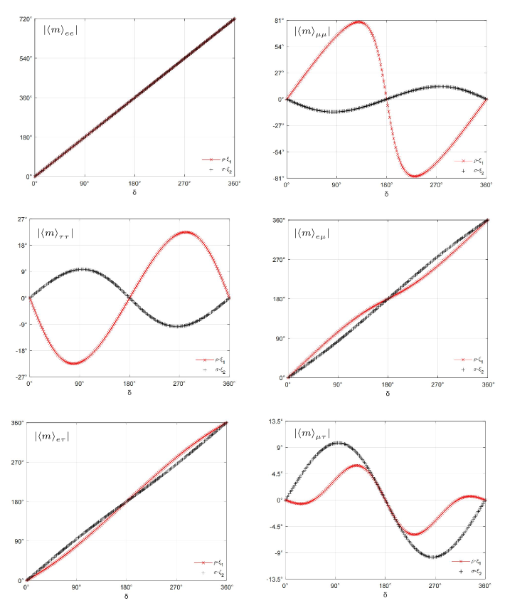
Figure 1: The variations of $\rho-\xi_{1}$ and $\sigma-\xi_{2}$ with respect to $\delta$ for each of $|\langle m\rangle_{\alpha\beta}|$ in the NMO case, where the best-fit values of three neutrino mixing angles have been input.

2.2 The upper and lower bounds of $|\langle m\rangle_{\alpha\beta}|$

Now we proceed to analytically determine the extremum of each $|\langle m\rangle_{\alpha\beta}|$ against the effective Majorana phase $\sigma$, which is related to $m_{2}$ and thus less sensitive to the mass ordering of three neutrinos. To this end, we express $|\langle m\rangle_{\alpha\beta}|$ in a generic way as follows:

$$|{\langle m\rangle_{\alpha\beta}}|=\left|r_{1}e^{{\rm i}\rho}+r_{2}e^{{\rm i}\sigma}+r_{3}\right|\;,$$ (12)

where $r_{i}\propto m_{i}$ (for $i=1,2,3$) are real. Allowing Eq. (12) to take its extremum with respect to $\sigma$,

$$\frac{\partial|{\langle m\rangle_{\alpha\beta}}|}{\partial\sigma}=0\;\;\Longrightarrow\;\;\frac{\displaystyle r_{1}r_{2}\sin\left(\rho-\sigma\right)-r_{2}r_{3}\sin\sigma}{\displaystyle\sqrt{r^{2}_{1}+r^{2}_{2}+r^{2}_{3}+2r_{1}r_{2}\cos\left(\rho-\sigma\right)+2r_{1}r_{3}\cos\rho+2r_{2}r_{3}\cos\sigma}}=0\;,$$ (13)

we obtain the condition

$$\tan\sigma=\frac{r_{1}\sin\rho}{r_{1}\cos{\rho}+r_{3}}\;,$$ (14)

which permits us to either maximize or minimize the magnitude of $|{\langle m\rangle_{\alpha\beta}}|$ for the given values of $\rho$ and $m_{1}$ (or $m_{3}$). Substituting Eq. (14) into Eq. (12), we immediately arrive at the upper (“U”) and lower (“L”) bounds of $|{\langle m\rangle_{\alpha\beta}}|$:

$$|{\langle m\rangle_{\alpha\beta}}|_{\rm U}=\Biggl{\lvert}{\left|r_{1}e^{{\rm i}\rho}+r_{3}\right|+r_{2}}\Biggr{\rvert}\;,$$

$$|{\langle m\rangle_{\alpha\beta}}|_{\rm L}=\Biggl{\lvert}{\left|r_{1}e^{{\rm i}\rho}+r_{3}\right|-r_{2}}\Biggr{\rvert}\;.\hskip 42.67912pt$$ (15)

These two bounds will help us a lot in determining the bulk of the parameter space of $|{\langle m\rangle_{\alpha\beta}}|$ for arbitrary values of $\rho$ and reasonable values of $m_{1}$ (or $m_{3}$). In this work we focus on $m_{i}\lesssim 0.1~{}{\rm eV}$, as conservatively constrained by current observational data [1].

To be more specific, we write out the upper and lower bounds for each of the six effective Majorana neutrino masses as follows.

• $|{\langle m\rangle_{ee}}|$. Defining $m^{ee}_{1}=m_{1}c^{2}_{12}c^{2}_{13}$, $m^{ee}_{2}=m_{2}s^{2}_{12}c^{2}_{13}$ and $m^{ee}_{3}=m_{3}s^{2}_{13}$, we have

  $$|{\langle m\rangle_{ee}}|_{\rm U,L}=\Biggl{\lvert}\left|m^{ee}_{1}e^{{\rm i}\rho}+m^{ee}_{3}\right|\pm m^{ee}_{2}\Biggr{\rvert}\;.\hskip 28.45274pt$$ (16)

• $|{\langle m\rangle_{\mu\mu}}|$. Defining $m^{\mu\mu}_{1}=m_{1}\left|\left(s_{12}c_{23}+c_{12}s_{23}s_{13}e^{{\rm i}\delta}\right)^{2}\right|$, $m^{\mu\mu}_{2}=m_{2}\left|\left(c_{12}c_{23}-s_{12}s_{23}s_{13}e^{{\rm i}\delta}\right)^{2}\right|$ and $m^{\mu\mu}_{3}=m_{3}c^{2}_{13}s^{2}_{23}$, we obtain

  $$|{\langle m\rangle_{\mu\mu}}|_{\rm U,L}=\Biggl{\lvert}\left|m^{\mu\mu}_{1}e^{{\rm i}\rho}+m^{\mu\mu}_{3}\right|\pm m^{\mu\mu}_{2}\Biggr{\rvert}\;.\hskip 28.45274pt$$ (17)

• $|{\langle m\rangle_{\tau\tau}}|$. Defining $m^{\tau\tau}_{1}=m_{1}\left|\left(s_{12}s_{23}-c_{12}c_{23}s_{13}e^{{\rm i}\delta}\right)^{2}\right|$, $m^{\tau\tau}_{2}=m_{2}\left|\left(c_{12}s_{23}+s_{12}c_{23}s_{13}e^{{\rm i}\delta}\right)^{2}\right|$ and $m^{\tau\tau}_{3}=m_{3}c^{2}_{13}c^{2}_{23}$, we arrive at

  $$|{\langle m\rangle_{\tau\tau}}|_{\rm U,L}=\Biggl{\lvert}\left|m^{\tau\tau}_{1}e^{{\rm i}\rho}+m^{\tau\tau}_{3}\right|\pm m^{\tau\tau}_{2}\Biggr{\rvert}\;.\hskip 28.45274pt$$ (18)

• $|{\langle m\rangle_{e\mu}}|$. Defining $m^{e\mu}_{1}=m_{1}c_{12}c_{13}\lvert{s_{12}c_{23}+c_{12}s_{23}s_{13}e^{{\rm i}\delta}}\rvert$, $m^{e\mu}_{2}=m_{2}s_{12}c_{13}\lvert{c_{12}c_{23}-s_{12}s_{23}s_{13}e^{{\rm i}\delta}}\rvert$ and $m^{e\mu}_{3}=m_{3}c_{13}s_{23}s_{13}$, we have

  $$|{\langle m\rangle_{e\mu}}|_{\rm U,L}=\Biggl{\lvert}\left|-m^{e\mu}_{1}e^{{\rm i}\rho}+m^{e\mu}_{3}\right|\pm m^{e\mu}_{2}\Biggr{\rvert}\;.\hskip 28.45274pt$$ (19)

• $|\left\langle m\rangle_{e\tau}\right|$. Defining $m^{e\tau}_{1}=m_{1}c_{12}c_{13}\left|s_{12}s_{23}-c_{12}c_{23}s_{13}e^{{\rm i}\delta}\right|$, $m^{e\tau}_{2}=m_{2}s_{12}c_{13}\left|c_{12}s_{23}+s_{12}c_{23}s_{13}e^{{\rm i}\delta}\right|$ and $m^{e\tau}_{3}=m_{3}c_{13}c_{23}s_{13}$, we obtain

  $$|{\langle m\rangle_{e\tau}}|_{\rm U,L}=\Biggl{\lvert}\left|m^{e\tau}_{1}e^{{\rm i}\rho}+m^{e\tau}_{3}\right|\pm m^{e\tau}_{2}\Biggr{\rvert}\;.\hskip 28.45274pt$$ (20)

• $|{\langle m\rangle_{\mu\tau}}|$. Let us define $m^{\mu\tau}_{1}=m_{1}\left|\left(s_{12}c_{23}+c_{12}s_{23}s_{13}e^{{\rm i}\delta}\right)\left(s_{12}s_{23}-c_{12}c_{23}s_{13}e^{{\rm i}\delta}\right)\right|$ together with $m^{\mu\tau}_{2}=m_{2}\left|\left(c_{12}c_{23}-s_{12}s_{23}s_{13}e^{{\rm i}\delta}\right)\left(c_{12}s_{23}+s_{12}c_{23}s_{13}e^{{\rm i}\delta}\right)\right|$ and $m^{\mu\tau}_{3}=m_{3}c^{2}_{13}c_{23}s_{23}$. Then

  $$|{\langle m\rangle_{\mu\tau}}|_{\rm U,L}=\Biggl{\lvert}\left|-m^{\mu\tau}_{1}e^{{\rm i}\rho}+m^{\mu\tau}_{3}\right|\pm m^{\mu\tau}_{2}\Biggr{\rvert}\;.\hskip 28.45274pt$$ (21)

These analytical results will be used in our numerical mapping of the 3D profiles of $|{\langle m\rangle_{\alpha\beta}}|$.

3 Numerical 3D mapping of $|{\langle m\rangle_{\alpha\beta}}|$

3.1 Normal mass ordering

In the NMO case (i.e., $m_{1}<m_{2}<m_{3}$) we choose the smallest neutrino mass $m_{1}$ as a free parameter. The other two neutrino masses can then be expressed as $m_{2}=\sqrt{{m^{2}_{1}}+\Delta m^{2}_{21}}$ and $m_{3}=\sqrt{{m^{2}_{1}}+\Delta m^{2}_{31}}$. With the help of Eqs. (16)—(21) and the best-fit values of $\Delta m^{2}_{21}$, $\Delta m^{2}_{31}$, $\theta_{12}$, $\theta_{13}$, $\theta_{23}$ and $\delta$ listed in section 2 [3], we plot the minimum and maximum of each of $|\langle m\rangle_{\alpha\beta}|$ with respect to the unknown phase parameter $\sigma$ by requiring the other unknown phase parameter $\rho$ and the unknown neutrino mass $m_{1}$ to vary in their respectively allowed regions. Our numerical results for the 3D profiles of $|\langle m\rangle_{\alpha\beta}|$ are shown in Fig. 2. Some explicit discussions are in order.

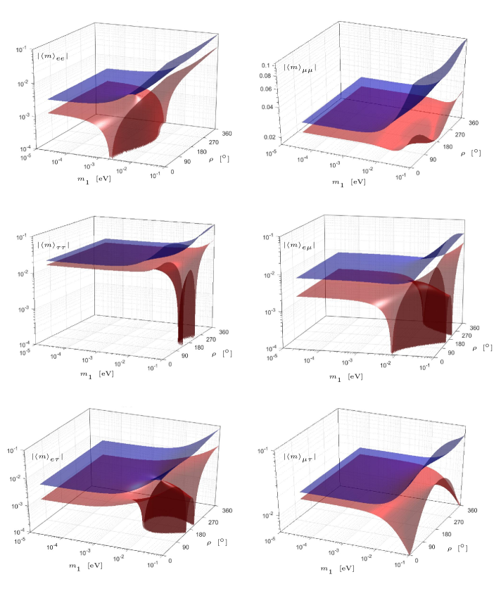
Figure 2: The 3D profile of each of the six effective Majorana neutrino masses $|\langle m\rangle_{\alpha\beta}|$ (for $\alpha,\beta=e,\mu,\tau$): its upper (blue) and lower (red) bounds are functions of $m_{1}$ and $\rho$ in the NMO case. Note that the two touching points between the upper and lower layers of $|\langle m\rangle_{e\mu}|$ are equivalent in physics, because they correspond to $\rho=0$ and $2\pi$.

3.1.1 The bounds of $|{\langle m\rangle_{ee}}|$

As shown in Fig. 2, there is a unique touching point between the upper and lower layers of $|{\langle m\rangle_{ee}}|$. The location of this interesting point can be analytically fixed from Eq. (16) by simply setting $|{\langle m\rangle_{ee}}|_{\rm U}=|{\langle m\rangle_{ee}}|_{\rm L}\equiv|{\langle m\rangle_{ee}}|_{*}$. The latter implies

$$m_{1}c^{2}_{12}c^{2}_{13}e^{{\rm i}\rho}+m_{3}s^{2}_{13}=0\;,$$ (22)

from which we immediately arrive at $\rho=\pi$,

$$m_{1}=\sqrt{\frac{\Delta m^{2}_{31}t^{4}_{13}}{c^{4}_{12}-t^{4}_{13}}}\simeq\sqrt{\Delta m^{2}_{31}}\hskip 2.84544pt\frac{t^{2}_{13}}{c^{2}_{12}}\;,$$ (23)

and

$$|{\langle m\rangle_{ee}}|_{*}=m_{2}s^{2}_{12}c^{2}_{13}\simeq\sqrt{\Delta m^{2}_{21}s^{4}_{12}c^{4}_{13}+\Delta m^{2}_{31}t^{4}_{12}s^{4}_{13}}\;,$$ (24)

where $t_{ij}\equiv\tan\theta_{ij}$ (for $ij=12,13,23$). Inputting the best-fit values of $\theta_{12}$, $\theta_{13}$, $\Delta m^{2}_{21}$ and $\Delta m^{2}_{31}$, we obtain $\left(\rho,m_{1}\right)_{*}\simeq\left(\pi,1.68~{}{\rm meV}\right)$ and $|{\langle m\rangle_{ee}}|_{*}\simeq 2.61~{}{\rm meV}$ for the touching point. In this special case the original Majorana phase $\xi_{1}$ is related to $\delta$ through $\xi_{1}=\pi-2\delta$.

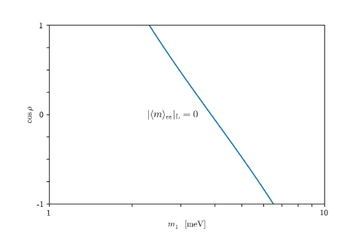
Figure 3: The correlation between $\cos\rho$ and $m_{1}$ constrained by $|{\langle m\rangle_{ee}}|_{\rm L}=0$ in the NMO case.

Note that $|{\langle m\rangle_{ee}}|_{\rm L}=0$ will hold if the condition

$$\cos\rho=\frac{\displaystyle\left(m^{2}_{2}s^{4}_{12}-m^{2}_{1}c^{4}_{12}\right)c^{4}_{13}-m^{2}_{3}s^{4}_{13}}{\displaystyle 2m_{1}m_{3}c^{2}_{12}c^{2}_{13}s^{2}_{13}}\;$$ (25)

is satisfied, as one can easily see from Eq. (16). This condition allows us to illustrate the specific correlation between $\cos\rho$ and $m_{1}$ in Fig. 3. It is clear that $|{\langle m\rangle_{ee}}|=0$ puts a strict constraint on the range of $m_{1}$, which approximately varies between $2~{}{\rm meV}$ and $7~{}{\rm meV}$.

3.1.2 The bounds of $|{\langle m\rangle_{\mu\mu}}|$

As is shown in Fig. 2, the upper and lower layers of $|{\langle m\rangle_{\mu\mu}}|$ are highly plain or flat for $m_{1}\lesssim 0.05~{}{\rm eV}$ and arbitrary values of $\rho$, and they have no intersecting point or area. For $m_{1}\lesssim 0.1~{}{\rm eV}$, the possibility of $|{\langle m\rangle_{\mu\mu}}|=0$ has been ruled out.

3.1.3 The bounds of $|{\langle m\rangle_{\tau\tau}}|$

Fig. 2 tells us that $|{\langle m\rangle_{\tau\tau}}|_{\rm L}$ is possible to vanish when $m_{1}$ and $\rho$ approach $0.1~{}{\rm eV}$ and $\pi$, respectively. Taking $|{\langle m\rangle_{\tau\tau}}|_{\rm L}=0$, we immediately arrive at

$$\cos\rho=\frac{m^{2}_{2}\left|\left(c_{12}s_{23}+s_{12}c_{23}s_{13}e^{\rm i\delta}\right)^{2}\right|^{2}-m^{2}_{1}\left|\left(s_{12}s_{23}-c_{12}c_{23}s_{13}e^{\rm i\delta}\right)^{2}\right|^{2}-m^{2}_{3}c^{4}_{13}c^{4}_{23}}{2m_{1}m_{3}c^{2}_{13}c^{2}_{23}\left|\left(s_{12}s_{23}-c_{12}c_{23}s_{13}e^{\rm i\delta}\right)^{2}\right|}\;$$ (26)

from Eq. (18). In this case the correlation between $\cos\rho$ and $m_{1}$ is illustrated in Fig. 4. It is obvious that $|{\langle m\rangle_{\tau\tau}}|_{\rm L}=0$ sets a lower limit for $m_{1}$ (roughly about $0.05~{}{\rm eV}$) and an upper limit for $\cos\rho$ (roughly around $-0.75$). Of course, these numerical observations depend closely on the best-fit inputs of current neutrino oscillation parameters, but they may at least give us a ball-park feeling of the interesting correlative behaviors of $m_{1}$ and $\cos\rho$ under the condition of $|{\langle m\rangle_{\tau\tau}}|_{\rm L}=0$ in the NMO case.

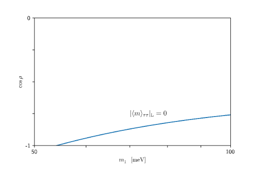
Figure 4: The correlation between $\cos\rho$ and $m_{1}$ constrained by $|{\langle m\rangle_{\tau\tau}}|_{\rm L}=0$ in the NMO case.

3.1.4 The bounds of $|{\langle m\rangle_{e\mu}}|$

Two features of the profile of $|{\langle m\rangle_{e\mu}}|$ in Fig. 2 are worthy of remarking. Similar to $|{\langle m\rangle_{\tau\tau}}|_{\rm L}$, the lower bound of $|{\langle m\rangle_{e\mu}}|$ is possible to vanish when $m_{1}$ is around $0.01~{}{\rm eV}$ or larger. On the other hand, the upper and lower limits of $|{\langle m\rangle_{e\mu}}|$ have a unique touching point fixed by the equality $|\langle m\rangle_{e\mu}|_{\rm U}=|\langle m\rangle_{e\mu}|_{\rm L}\equiv|\langle m\rangle_{e\mu}|_{*}$ or equivalently the condition

$$-m_{1}e^{\rm i\rho}c_{12}\left|s_{12}c_{23}+c_{12}s_{23}s_{13}e^{\rm i\delta}\right|+m_{3}s_{13}s_{23}=0\;.$$ (27)

So it is straightforward for us to obtain $\rho=0$ (or $2\pi$) from Eq. (27), together with

$$m_{1}=\sqrt{\frac{\Delta m^{2}_{31}s^{2}_{13}s^{2}_{23}}{\displaystyle c^{2}_{12}\lvert{s_{12}c_{23}+c_{12}s_{23}s_{13}e^{\rm i\delta}}\rvert^{2}-s^{2}_{13}s^{2}_{23}}}\;,$$ (28)

and

$$|{\langle m\rangle_{e\mu}}|_{*}=m_{2}s_{12}c_{13}\left|c_{12}c_{23}-s_{12}s_{23}s_{13}e^{{\rm i}\delta}\right|=\sqrt{m^{2}_{1}+\Delta m^{2}_{21}}\hskip 1.42271pts_{12}c_{13}\left|c_{12}c_{23}-s_{12}s_{23}s_{13}e^{{\rm i}\delta}\right|\;.$$ (29)

Numerically, we find $(\rho,m_{1})\simeq(0,0.0289~{}{\rm eV})$ and $|{\langle m\rangle_{e\mu}}|_{*}\simeq 9.88~{}{\rm meV}$ for the touching point, where the original Majorana phase $\xi_{1}$ reads as $\xi_{1}=-\arg\left(s_{12}c_{23}+c_{12}s_{23}s_{13}e^{\rm i\delta}\right)-\delta$.

Moreover, $|{\langle m\rangle_{e\mu}}|_{\rm L}=0$ can be obtained if the condition

$$\cos\rho=\frac{m^{2}_{3}s^{2}_{13}s^{2}_{23}+m^{2}_{1}c^{2}_{12}|s_{12}c_{23}+c_{12}s_{23}s_{13}e^{\rm i\delta}|^{2}-m^{2}_{2}s^{2}_{12}|c_{12}c_{23}-s_{12}s_{23}s_{13}e^{\rm i\delta}|^{2}}{2m_{1}m_{3}c_{12}s_{13}s_{23}|s_{12}c_{23}+c_{12}s_{23}s_{13}e^{\rm i\delta}|}$$ (30)

is satisfied. A numerical illustration of this condition is presented in Fig. 5, from which one may also read out the lower bounds of $m_{1}$ and $\cos\rho$ for $|{\langle m\rangle_{e\mu}}|_{\rm L}=0$.

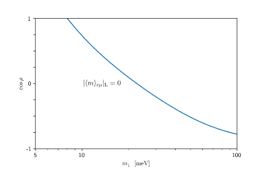
Figure 5: The correlation between $\cos\rho$ and $m_{1}$ constrained by $|{\langle m\rangle_{e\mu}}|_{\rm L}=0$ in the NMO case.

3.1.5 The bounds of $|{\langle m\rangle_{e\tau}}|$

Fig. 2 shows that the 3D profile of $|{\langle m\rangle_{e\tau}}|$ has an interesting bullet-like structure, whose tip is just the touching point between the layers of $|{\langle m\rangle_{e\tau}}|_{\rm U}$ and $|{\langle m\rangle_{e\tau}}|_{\rm L}$. In addition, one can clearly see that $|{\langle m\rangle_{e\tau}}|$ is possible to vanish when $\rho$ and $m_{1}$ take some appropriate values. The equality $|{\langle m\rangle_{e\tau}}|_{\rm U}=|{\langle m\rangle_{e\tau}}|_{\rm L}\equiv|{\langle m\rangle_{e\tau}}|_{*}$ requires

$$m_{1}e^{\rm i\rho}c_{12}\lvert s_{12}s_{23}-c_{12}c_{23}s_{13}e^{\rm i\delta}\rvert+m_{3}s_{13}c_{23}=0\;$$ (31)

to hold. As a result, the touching point is fixed by $\rho=\pi$ and

$$m_{1}=\sqrt{\frac{\Delta m^{2}_{31}s^{2}_{13}c^{2}_{23}}{\displaystyle c^{2}_{12}\lvert s_{12}s_{23}-c_{12}c_{23}s_{13}e^{\rm i\delta}\rvert^{2}-s^{2}_{13}c^{2}_{23}}}\;,$$ (32)

and thus

$$|{\langle m\rangle_{e\tau}}|_{*}=m_{2}s_{12}c_{13}\lvert{c_{12}s_{23}+s_{12}c_{23}s_{13}e^{\rm i\delta}}\rvert=\sqrt{m^{2}_{1}+\Delta m^{2}_{21}}\hskip 1.42271pts_{12}c_{13}\lvert{c_{12}s_{23}+s_{12}c_{23}s_{13}e^{{\rm i}\delta}}\rvert\;.$$ (33)

Comparing Eqs. (32) and (33) with Eqs. (28) and (29), we find that the former can be easily acquired from the latter by making the replacements $c_{23}\to s_{23}$ and $s_{23}\to-c_{23}$. This observation implies a kind of (approximate) $\mu$-$\tau$ interchange symmetry between $|{\langle m\rangle_{e\mu}}|$ and $|{\langle m\rangle_{e\tau}}|$, given the fact of $\theta_{23}\simeq\pi/4$ as indicated by current neutrino oscillation data [19]. Numerically, we have $(\rho,m_{1})\simeq(\pi,0.0124~{}{\rm eV})$ and $|{\langle m\rangle_{e\tau}}|_{*}\simeq 4.69{~{}\rm meV}$ for the touching point, where the original Majorana phase $\xi_{1}$ is related to $\delta$ through the relation $\xi_{1}=\pi-\arg\left(s_{12}s_{23}-c_{12}c_{23}s_{13}e^{\rm i\delta}\right)-\delta$.

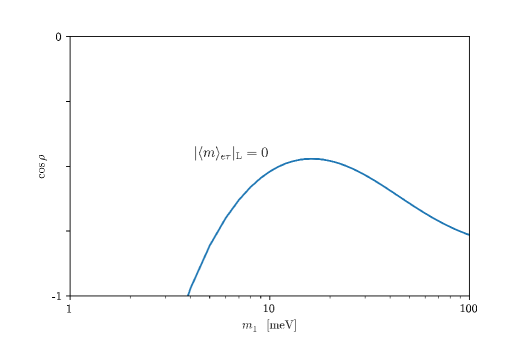
Figure 6: The correlation between $\cos\rho$ and $m_{1}$ constrained by $|{\langle m\rangle_{e\tau}}|_{\rm L}=0$ in the NMO case.

On the other hand, $|{\langle m\rangle_{e\tau}}|_{\rm L}=0$ will hold under the condition of

$$\cos\rho=\frac{\displaystyle m^{2}_{2}s^{2}_{12}|c_{12}s_{23}+s_{12}c_{23}s_{13}e^{\rm i\delta}|^{2}-m^{2}_{3}c^{2}_{23}s^{2}_{13}-m^{2}_{1}c^{2}_{12}|s_{12}s_{23}-c_{12}c_{23}s_{13}e^{\rm i\delta}|^{2}}{\displaystyle 2m_{1}m_{3}c_{12}s_{13}c_{23}|s_{12}s_{23}-c_{12}c_{23}s_{13}e^{\rm i\delta}|}\;.$$ (34)

A numerical illustration of this condition is shown in Fig. 6, in which one can see a lower bound $m_{1}\gtrsim 4~{}{\rm meV}$ as required by $|{\langle m\rangle_{e\tau}}|_{\rm L}=0$.

3.1.6 The bounds of $|{\langle m\rangle_{\mu\tau}}|$

Quite similar to the 3D profile of $|{\langle m\rangle_{\mu\mu}}|$ discussed above, the upper and lower layers of $|{\langle m\rangle_{\mu\tau}}|$ are highly plain and have no intersecting point or area, as shown in Fig. 2. For $m_{1}\lesssim 0.1~{}{\rm eV}$, the possibility of $|{\langle m\rangle_{\mu\tau}}|=0$ has already been excluded.

3.2 Inverted mass ordering

In the IMO case (i.e., $m_{3}<m_{1}<m_{2}$), we have the relations $m_{1}=\sqrt{{m^{2}_{3}}-\Delta m^{2}_{32}-\Delta m^{2}_{21}}$ and $m_{2}=\sqrt{{m^{2}_{3}}-\Delta m^{2}_{32}}$ with $\Delta m^{2}_{21}$ and $\Delta m^{2}_{32}$ having been extracted from current neutrino oscillation data [3]. So let us choose the smallest neutrino mass $m_{3}$, together with the effective Majorana phase $\rho$, to describe the profiles of $|\langle m\rangle_{\alpha\beta}|$. Since the upper and lower bounds of $|\langle m\rangle_{\alpha\beta}|$ against the other Majorana phase $\sigma$ have been determined in Eqs. (16)—(21), here we numerically illustrate their 3D profiles in Fig. 7. More concrete discussions are in order.

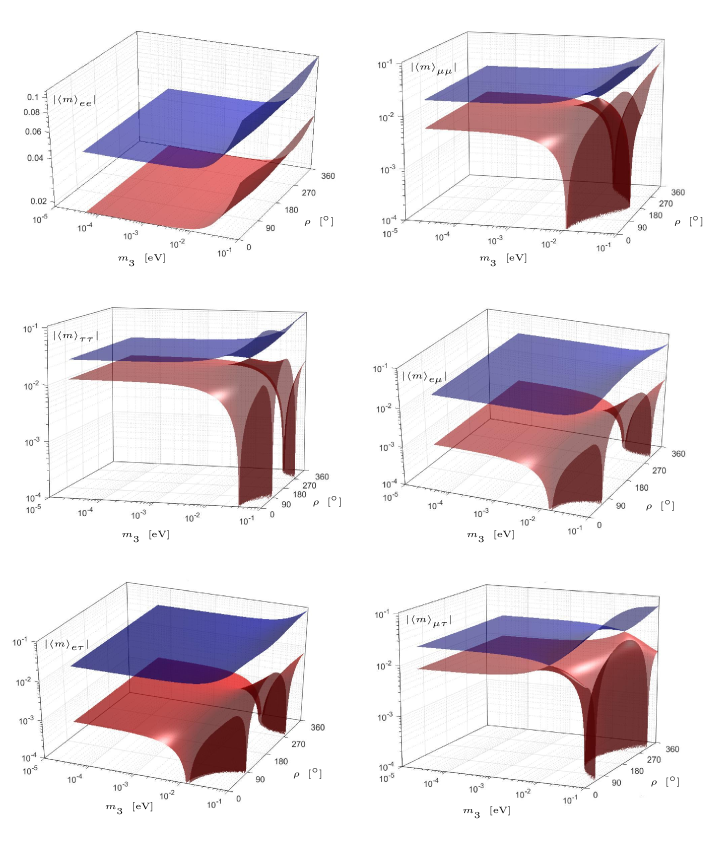
Figure 7: The 3D profile of each of the six effective Majorana neutrino masses $|\langle m\rangle_{\alpha\beta}|$ (for $\alpha,\beta=e,\mu,\tau$): its upper (blue) and lower (red) bounds are functions of $m_{3}$ and $\rho$ in the IMO case. Note that the two touching points between the upper and lower layers of $|\langle m\rangle_{\mu\tau}|$ are equivalent in physics, because they correspond to $\rho=0$ and $2\pi$.

3.2.1 The bounds of $|{\langle m\rangle_{ee}}|$

As shown in Fig. 7, the lower and upper layers of $|{\langle m\rangle_{ee}}|$ are essentially flat, stable, parallel to each other and insensitive to the changes of $\rho$; and their magnitudes are around $0.01~{}{\rm eV}$ and $0.1~{}{\rm eV}$, respectively, when $m_{3}\lesssim 0.01~{}{\rm eV}$ holds. These interesting features are quite different from those salient features of $|{\langle m\rangle_{ee}}|$ in the NMO case, where the parameter space of $|{\langle m\rangle_{ee}}|$ is rather tricky and even $|{\langle m\rangle_{ee}}|=0$ is possible.

It is optimistically expected that the next-generation $0\nu 2\beta$ experiments might be able to probe the IMO possibility of massive neutrinos if their sensitivities to the half-lives of the decaying isotopes (such as ${}^{76}_{32}{\rm Ge}$, ${}^{136}_{~{}54}{\rm Xe}$ and ${}^{130}_{~{}52}{\rm Te}$) can finally reach the level of $10^{27}$ or even $10^{28}$ years [20, 21]. But a global analysis of today’s neutrino oscillation data indicates that the NMO possibility seems to be slightly favored [22]. The next-generation neutrino oscillation experiments, especially JUNO, DUNE and Hyper-Kamiokande [1] will determine the neutrino mass ordering and thus greatly reduce the uncertainties of $|{\langle m\rangle_{\alpha\beta}}|$ under discussion.

3.2.2 The bounds of $|{\langle m\rangle_{\mu\mu}}|$

Fig. 7 tells us that the profile of $|{\langle m\rangle_{\mu\mu}}|$ in the IMO case is highly nontrivial as compared with that in the NMO case. Namely, $|{\langle m\rangle_{\mu\mu}}|_{\rm U}$ and $|{\langle m\rangle_{\mu\mu}}|_{\rm L}$ have a touching point, and $|{\langle m\rangle_{\mu\mu}}|_{\rm L}$ is possible to vanish. Taking $|{\langle m\rangle_{\mu\mu}}|_{\rm U}=|{\langle m\rangle_{\mu\mu}}|_{\rm L}\equiv|{\langle m\rangle_{\mu\mu}}|_{*}$, we find that the touching point can be determined from the condition

$$m_{1}e^{\rm i\rho}\left|\left(s_{12}c_{23}+c_{12}s_{23}s_{13}e^{\rm i\delta}\right)^{2}\right|+m_{3}{c^{2}_{13}}{s^{2}_{23}}=0\;.$$ (35)

It is then straightforward to obtain $\rho=\pi$,

$$m_{3}=\frac{\displaystyle\sqrt{-\Delta m^{2}_{32}-\Delta m^{2}_{21}}\left|\left(s_{12}c_{23}+c_{12}s_{23}s_{13}e^{\rm i\delta}\right)^{2}\right|}{\displaystyle\sqrt{c^{4}_{13}s^{4}_{23}-\left|\left(s_{12}c_{23}+c_{12}s_{23}s_{13}e^{\rm i\delta}\right)^{2}\right|^{2}}}\;,$$ (36)

and

$$|{\langle m\rangle_{\mu\mu}}|_{*}=m_{2}\left|\left(c_{12}c_{23}-s_{12}s_{23}s_{13}e^{\rm i\delta}\right)^{2}\right|=\sqrt{m^{2}_{3}-\Delta m^{2}_{32}}\left|\left(c_{12}c_{23}-s_{12}s_{23}s_{13}e^{\rm i\delta}\right)^{2}\right|\;,$$ (37)

where $\Delta m^{2}_{32}<0$. Numerically, we have $\left(\rho,m_{3}\right)\simeq\left(\pi,0,0143~{}{\rm eV}\right)$ and $|{\langle m\rangle_{\mu\mu}}|_{*}\simeq 0.0146~{}{\rm eV}$ for the touching point. At this point the original Majorana phase $\xi_{1}$ is related to the Dirac phase $\delta$ via the relation $\xi_{1}=\pi-\arg\left[\left(s_{12}c_{23}+c_{12}s_{23}s_{13}e^{\rm i\delta}\right)^{2}\right]$.

In addition, let us consider the possibility of vanishing $|{\langle m\rangle_{\mu\mu}}|$. We find that $|{\langle m\rangle_{\mu\mu}}|_{\rm L}=0$ will be achieved if the condition

$$\cos\rho=\frac{\displaystyle m^{2}_{2}\left|\left(c_{12}c_{23}-s_{12}s_{23}s_{13}e^{\rm i\delta}\right)^{2}\right|^{2}-m^{2}_{1}\left|\left(s_{12}c_{23}+c_{12}s_{23}s_{13}e^{\rm i\delta}\right)^{2}\right|^{2}-m^{2}_{3}c^{4}_{13}s^{4}_{23}}{\displaystyle 2m_{1}m_{3}c^{2}_{13}s^{2}_{23}\left|\left(s_{12}c_{23}+c_{12}s_{23}s_{13}e^{\rm i\delta}\right)^{2}\right|}$$ (38)

is satisfied. A numerical illustration of this condition is given in Fig. 8, from which one can see $0.01~{}{\rm eV}\lesssim m_{3}\lesssim 0.06~{}{\rm eV}$ as constrained by $|{\langle m\rangle_{\mu\mu}}|_{\rm L}=0$.

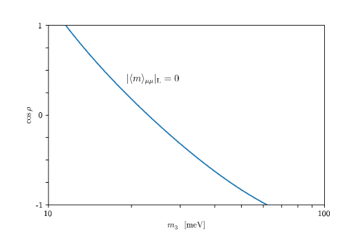
Figure 8: The correlation between $\cos\rho$ and $m_{3}$ constrained by $|{\langle m\rangle_{\mu\mu}}|_{\rm L}=0$ in the IMO case.

3.2.3 The bounds of $|{\langle m\rangle_{\tau\tau}}|$

Fig. 7 shows that the 3D profile of $|{\langle m\rangle_{\tau\tau}}|$ is quite similar to that of $|{\langle m\rangle_{\mu\mu}}|$ in the IMO case, implying an approximate $\mu$-$\tau$ symmetry between them. The location of the touching point between the upper and lower layer of $|{\langle m\rangle_{\tau\tau}}|$ can be fixed by taking $|{\langle m\rangle_{\tau\tau}}|_{\rm U}=|{\langle m\rangle_{\tau\tau}}|_{\rm L}\equiv|{\langle m\rangle_{\tau\tau}}|_{*}$, namely

$$m_{1}e^{\rm i\rho}\left|\left(s_{12}s_{23}-c_{12}c_{23}s_{13}e^{\rm i\delta}\right)^{2}\right|+m_{3}{c^{2}_{13}}{c^{2}_{23}}=0\;.$$ (39)

As a result, we arrive at $\rho=\pi$,

$$m_{3}=\frac{\displaystyle\sqrt{-\Delta m^{2}_{32}-\Delta m^{2}_{21}}\left|\left(s_{12}s_{23}-c_{12}c_{23}s_{13}e^{\rm i\delta}\right)^{2}\right|}{\displaystyle\sqrt{c^{4}_{13}c^{4}_{23}-\left|\left(s_{12}s_{23}-c_{12}c_{23}s_{13}e^{\rm i\delta}\right)^{2}\right|^{2}}}\;,$$ (40)

and

$$|{\langle m\rangle_{\tau\tau}}|_{*}=m_{2}\left|\left(c_{12}s_{23}+s_{12}c_{23}s_{13}e^{\rm i\delta}\right)^{2}\right|=\sqrt{m^{2}_{3}-\Delta m^{2}_{32}}\left|\left(c_{12}s_{23}+s_{12}c_{23}s_{13}e^{\rm i\delta}\right)^{2}\right|\;$$ (41)

from Eq. (39). Numerically, $\left(\rho,m_{3}\right)\simeq\left(\pi,0.0209~{}{\rm eV}\right)$ and $|{\langle m\rangle_{\tau\tau}}|_{*}\simeq 0.0228~{}{\rm eV}$ for the touching point. As for the original Majorana phase at this point, $\xi_{1}=\pi-\arg\left[\left(s_{12}s_{23}-c_{12}c_{23}s_{13}e^{\rm i\delta}\right)^{2}\right]$.

Now that Eqs. (39)—(41) can be directly achieved from Eqs. (35)—(37) by making the replacements $c_{23}\to s_{23}$ and $s_{23}\to-c_{23}$, we may simply write out the condition for $|{\langle m\rangle_{\tau\tau}}|_{\rm L}=0$ with the help of Eq. (38) by making the same replacements. That is, $|{\langle m\rangle_{\tau\tau}}|_{\rm L}=0$ will hold if

$$\cos\rho=\frac{\displaystyle m^{2}_{2}\left|\left(c_{12}s_{23}+s_{12}c_{23}s_{13}e^{\rm i\delta}\right)^{2}\right|^{2}-m^{2}_{1}\left|\left(s_{12}s_{23}-c_{12}c_{23}s_{13}e^{\rm i\delta}\right)^{2}\right|^{2}-m^{2}_{3}c^{4}_{13}c^{4}_{23}}{\displaystyle 2m_{1}m_{3}c^{2}_{13}c^{2}_{23}\left|\left(s_{12}s_{23}-c_{12}c_{23}s_{13}e^{\rm i\delta}\right)^{2}\right|}\;$$ (42)

is satisfied. This condition is formally the same as that obtained in Eq. (26) for the NMO case. A numerical illustration of Eq. (42) is presented in Fig. 9. We immediately see that $m_{3}\gtrsim 0.04~{}{\rm eV}$ is required for $|{\langle m\rangle_{\tau\tau}}|_{\rm L}$ to vanish in the IMO case.

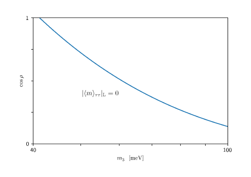
Figure 9: The correlation between $\cos\rho$ and $m_{3}$ constrained by $|{\langle m\rangle_{\tau\tau}}|_{\rm L}=0$ in the IMO case.

3.2.4 The bounds of $|{\langle m\rangle_{e\mu}}|$

Comparing between the 3D profile of $|{\langle m\rangle_{e\mu}}|$ in the NMO case shown in Fig. 2 and that in the IMO case shown in Fig. 7, we find that the latter is somewhat less structured (e.g., its upper and lower layers have no touching or intersecting point in the given parameter space). But in both cases $|{\langle m\rangle_{e\mu}}|_{\rm L}$ is possible to vanish.

The specific condition for $|{\langle m\rangle_{e\mu}}|_{\rm L}=0$ has been given in Eq. (30), but now it is subject to the IMO case and thus yields a different curve as illustrated by Fig. 10. One can see that $|{\langle m\rangle_{e\mu}}|_{\rm L}=0$ requires the smallest neutrino mass $m_{3}$ to lie in the range of $m_{3}\gtrsim 0.01~{}{\rm eV}$.

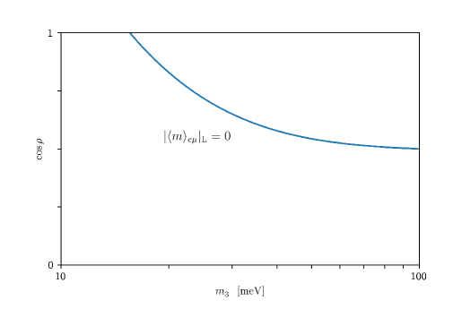
Figure 10: The correlation between $\cos\rho$ and $m_{3}$ constrained by $|{\langle m\rangle_{e\mu}}|_{\rm L}=0$ in the IMO case.

3.2.5 The bounds of $|{\langle m\rangle_{e\tau}}|$

As shown in Fig. 7, the 3D profile of $|{\langle m\rangle_{e\tau}}|$ with its upper and lower layers exhibits a striking similarity to that of $|{\langle m\rangle_{e\mu}}|$ in the IMO case. This interesting feature demonstrates the existence of an approximate $\mu$-$\tau$ symmetry between these two effective Majorana neutrino masses as supported by current neutrino oscillation data [19].

Similarly, $|{\langle m\rangle_{e\tau}}|_{\rm L}=0$ will hold if the condition presented in Eq. (34) is satisfied in the IMO case. The corresponding numerical illustration of this condition is shown in Fig. 11, which is quite similar to Fig. 10 as a direct consequence of the approximate $\mu$-$\tau$ symmetry mentioned above. It is obvious that $m_{3}\gtrsim 0.01~{}{\rm eV}$ is required to obtain $|{\langle m\rangle_{e\tau}}|_{\rm L}=0$.

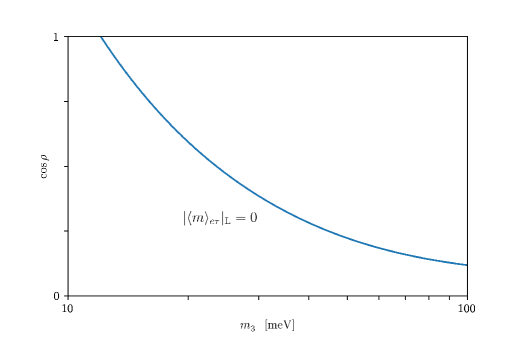
Figure 11: The correlation between $\cos\rho$ and $m_{3}$ constrained by $|{\langle m\rangle_{e\tau}}|_{\rm L}=0$ in the IMO case.

3.2.6 The bounds of $|{\langle m\rangle_{\mu\tau}}|$

As shown in Fig. 7, the upper and lower layers of $|{\langle m\rangle_{\mu\tau}}|$ have a touching point determined by the condition $|{\langle m\rangle_{\mu\tau}}|_{\rm U}=|{\langle m\rangle_{\mu\tau}}|_{\rm L}\equiv|{\langle m\rangle_{\mu\tau}}|_{*}$. The latter means

$$-m_{1}e^{\rm i\rho}\left|\left(s_{12}c_{23}+c_{12}s_{23}s_{13}e^{\rm i\delta}\right)\left(s_{12}s_{23}-c_{12}c_{23}s_{13}e^{\rm i\delta}\right)\right|+m_{3}c^{2}_{13}c_{23}s_{23}=0\;,$$ (43)

from which we arrive at $\rho=0$ (or $2\pi$),

$$m_{3}=\frac{\displaystyle\sqrt{-\Delta m^{2}_{32}-\Delta m^{2}_{21}}\left|\left(s_{12}c_{23}+c_{12}s_{23}s_{13}e^{\rm i\delta}\right)\left(s_{12}s_{23}-c_{12}c_{23}s_{13}e^{\rm i\delta}\right)\right|}{\displaystyle\sqrt{c^{4}_{13}c^{2}_{23}s^{2}_{23}-\left|\left(s_{12}c_{23}+c_{12}s_{23}s_{13}e^{\rm i\delta}\right)\left(s_{12}s_{23}-c_{12}c_{23}s_{13}e^{\rm i\delta}\right)\right|^{2}}}\;,$$ (44)

and thus

$$|{\langle m\rangle_{\mu\tau}}|_{*} = m_{2}\left|\left(c_{12}c_{23}-s_{12}s_{23}s_{13}e^{{\rm i}\delta}\right)\left(c_{12}s_{23}+s_{12}c_{23}s_{13}e^{{\rm i}\delta}\right)\right|$$ (45)

$$= \sqrt{m^{2}_{3}-\Delta m^{2}_{32}}\left|\left(c_{12}c_{23}-s_{12}s_{23}s_{13}e^{{\rm i}\delta}\right)\left(c_{12}s_{23}+s_{12}c_{23}s_{13}e^{{\rm i}\delta}\right)\right|\;.\hskip 14.22636pt$$

Numerically, we obtain $(\rho,m_{3})\simeq(0,0.0172~{}{\rm eV})$ and $|{\langle m\rangle_{\mu\tau}}|_{*}\simeq 0.0182~{}{\rm eV}$ for the touching point. At this point we are left with $\xi_{1}=-\arg\left[\left(s_{12}c_{23}+c_{12}s_{23}s_{13}e^{\rm i\delta}\right)\left(s_{12}s_{23}-c_{12}c_{23}s_{13}e^{\rm i\delta}\right)\right]$ which links the original Majorana phase $\xi_{1}$ to the Dirac phase $\delta$.

On the other hand, $|{\langle m\rangle_{\mu\tau}}|_{\rm L}=0$ will hold if the condition

$$\cos\rho = \frac{\displaystyle m^{2}_{3}c^{4}_{13}c^{2}_{23}s^{2}_{23}+m^{2}_{1}\left|\left(s_{12}c_{23}+c_{12}s_{23}s_{13}e^{\rm i\delta}\right)\left(s_{12}s_{23}-c_{12}c_{23}s_{13}e^{\rm i\delta}\right)\right|^{2}}{\displaystyle 2m_{1}m_{3}c^{2}_{13}c_{23}s_{23}\left|\left(s_{12}c_{23}+c_{12}s_{23}s_{13}e^{\rm i\delta}\right)\left(s_{12}s_{23}-c_{12}c_{23}s_{13}e^{\rm i\delta}\right)\right|}$$ (46)

$$-\frac{\displaystyle m^{2}_{2}\left|\left(c_{12}c_{23}-s_{12}s_{23}s_{13}e^{{\rm i}\delta}\right)\left(c_{12}s_{23}+s_{12}c_{23}s_{13}e^{{\rm i}\delta}\right)\right|^{2}}{\displaystyle 2m_{1}m_{3}c^{2}_{13}c_{23}s_{23}\left|\left(s_{12}c_{23}+c_{12}s_{23}s_{13}e^{\rm i\delta}\right)\left(s_{12}s_{23}-c_{12}c_{23}s_{13}e^{\rm i\delta}\right)\right|}\;\hskip 14.22636pt$$

is satisfied. This condition is numerically illustrated in Fig 12, where one can see $m_{3}\gtrsim 0.02~{}{\rm eV}$ should hold as required by $|{\langle m\rangle_{\mu\tau}}|_{\rm L}=0$.

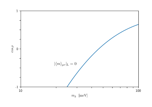
Figure 12: The correlation between $\cos\rho$ and $m_{3}$ constrained by $|{\langle m\rangle_{e\tau}}|_{\rm L}=0$ in the IMO case.

4 Some further discussions

So far we have discussed the 3D profiles of all the six independent effective Majorana neutrino masses $|\langle m\rangle_{\alpha\beta}|$ with respect to the effective Majorana phase $\rho$ and the smallest neutrino mass $m_{1}$ (or $m_{3}$) in the NMO (or IMO) case, where the other effective Majorana phase $\sigma$ has been eliminated by determining the upper and lowers bounds of each $|\langle m\rangle_{\alpha\beta}|$ against its corresponding $\sigma$. Such a phenomenological strategy is of course imperfect, but it can help a lot in simplifying our analytical and numerical descriptions of $|\langle m\rangle_{\alpha\beta}|$. Compared with the conventional 2D plots of $|\langle m\rangle_{\alpha\beta}|$ against $m_{1}$ or $m_{3}$, where all the CP-violating phases of the PMNS matrix $U$ are allowed to vary in their respective ranges, this 3D mapping of $|\langle m\rangle_{\alpha\beta}|$ is at least advantageous in the aspects of unraveling the dependence of each effective Majorana mass on its phase parameter $\rho$ and giving us a ball-park feeling of the bulk of its 3D parameter space.

In this respect we are going to further discuss the following three issues: (1) the possibility of a four-dimensional (4D) description of $|\langle m\rangle_{\alpha\beta}|$ with respect to $m_{1}$ (or $m_{3}$), $\rho$ and $\sigma$; (2) the arbitrariness in defining the two effective Majorana phases of $|\langle m\rangle_{\alpha\beta}|$; and (3) possible texture zeros and (or) an approximate $\mu$-$\tau$ symmetry hidden in the effective Majorana neutrino mass matrix $M_{\nu}$ as revealed in our analyses made above.

4.1 The 4D plots of $|\langle m\rangle_{\alpha\beta}|$

Fig. 13 shows the 4D plots of $|\langle m\rangle_{\alpha\beta}|$ with respect to the three free parameters $m_{1}$, $\rho$ and $\sigma$ in the NMO case, and Fig. 14 illustrates the similar plots as functions of $m_{3}$, $\rho$ and $\sigma$ in the IMO case. One can clearly see that the bigger $m_{1}$ (or $m_{3}$) goes, the bigger $|\langle m\rangle_{\alpha\beta}|$ will be. Judging from the color bar code attached to every plot in Figs. 13 and 14, one may roughly figure out the allowed range of $|\langle m\rangle_{\alpha\beta}|$. In the NMO case, for instance, it is the matrix element $|{\langle m\rangle_{\mu\mu}}|$ that has a lower bound of ${\cal O}(0.01)$ eV no matter how small $m_{1}$ is, while all the other five matrix elements are possible to vanish. As for the IMO case, one may similarly observe that the matrix element $|{\langle m\rangle_{ee}}|$ has no chance to vanish, but the other five matrix elements are possible to vanish.

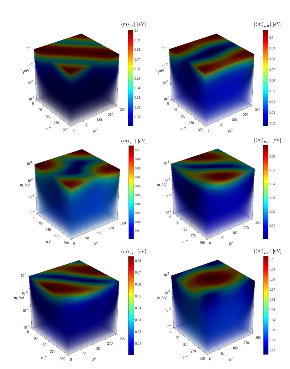
Figure 13: The 4D plot of each of the six effective Majorana neutrino masses $|\langle m\rangle_{\alpha\beta}|$ (for $\alpha,\beta=e,\mu,\tau$) with respect to $m_{1}$, $\rho$ and $\sigma$ in the NMO case.

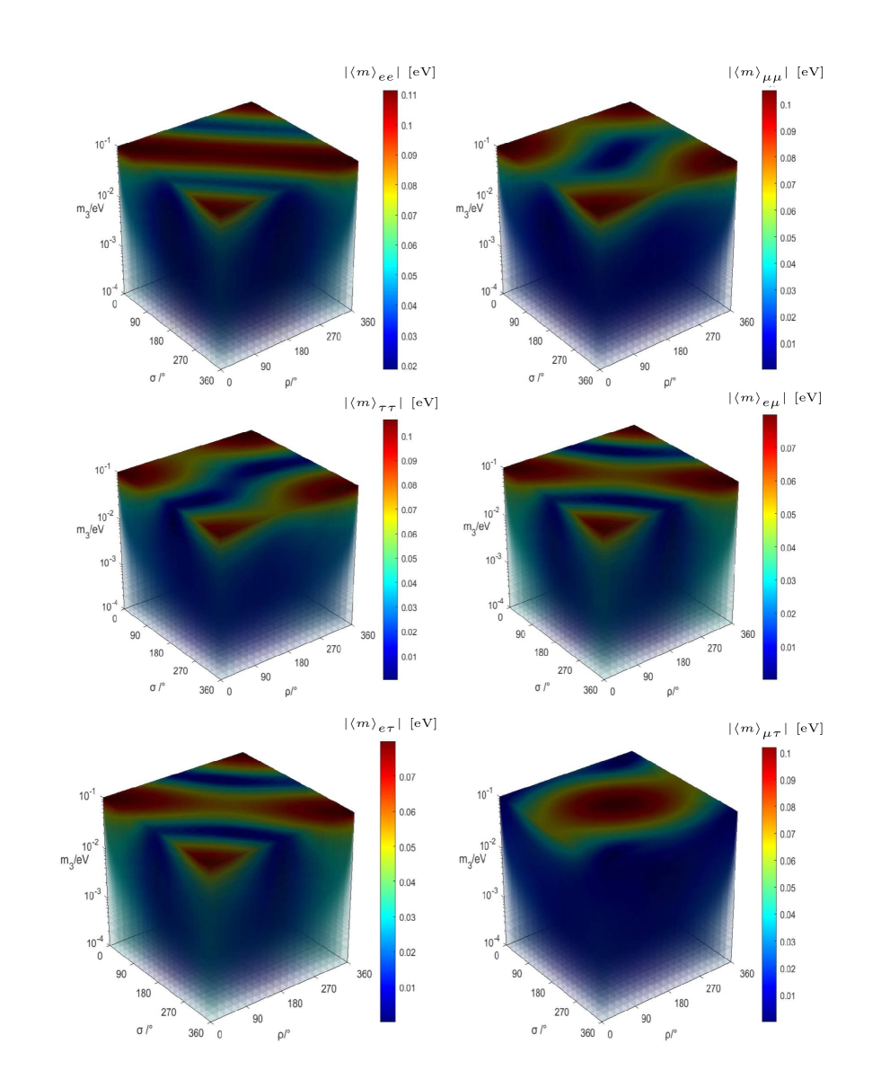
Figure 14: The 4D plot of each of the six effective Majorana neutrino masses $|\langle m\rangle_{\alpha\beta}|$ (for $\alpha,\beta=e,\mu,\tau$) with respect to $m_{3}$, $\rho$ and $\sigma$ in the IMO case.

We have to admit that the 3D mapping of $|{\langle m\rangle_{\alpha\beta}}|$ presented in Fig. 2 or Fig. 7 is much simpler and more transparent than its 4D analogue shown in Fig. 13 or Fig. 14. That is why we have focused on the 3D profiles of $|{\langle m\rangle_{\alpha\beta}}|$ and their salient features in this work.

4.2 On the effective Majorana phases of $|\langle m\rangle_{\alpha\beta}|$

In section 2.1 we have assigned the effective Majorana phases $\rho$ and $\sigma$ to the terms of $|{\langle m\rangle_{\alpha\beta}}|$ that are associated respectively with $m_{1}$ and $m_{2}$. The upper and lower bounds of $|{\langle m\rangle_{\alpha\beta}}|$ with respect to $\sigma$ are accordingly determined in section 2.2. Of course, there is always a degree of arbitrariness about such a phase assignment. In Refs. [15, 16, 17], for example, $\rho$ and $\sigma$ were assigned to the components of $|{\langle m\rangle_{ee}}|$ that are proportional respectively to $m_{1}$ and $m_{3}$. This different phase assignment leads us to $\rho=\xi_{1}-\xi_{2}$ and $\sigma=-\xi_{2}-2\delta$ for $|{\langle m\rangle_{ee}}|$, and the upper and lower limits of $|{\langle m\rangle_{ee}}|$ with respect to $\sigma$ turn out to be [16]

$$|{\langle m\rangle_{ee}}|_{\rm U,L}=\Biggl{\lvert}\left|m^{ee}_{1}e^{{\rm i}\rho}+m^{ee}_{2}\right|\pm m^{ee}_{3}\Biggr{\rvert}\;,$$ (47)

where $m^{ee}_{1}=m_{1}c^{2}_{12}c^{2}_{13}$, $m^{ee}_{2}=m_{2}s^{2}_{12}c^{2}_{13}$ and $m^{ee}_{3}=m_{3}s^{2}_{13}$ have been defined just above Eq. (16). In this case the 3D profile of $|{\langle m\rangle_{ee}}|$ for either the NMO or the IMO is shown in Fig. 15, a result consistent with the one obtained previously in Refs. [16, 17].

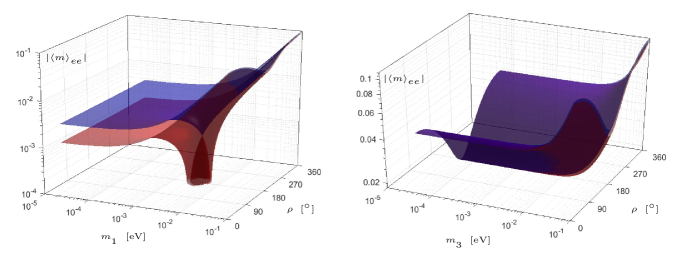
Figure 15: The 3D profile of $|{\langle m\rangle_{ee}}|$ in either the NMO case (left panel) or the IMO case (right panel) based on the phase assignment made in Eq. (47): its upper (blue) and lower (red) bounds are functions of $m_{1}$ (or $m_{3}$) and $\rho$.

Comparing the left panel of Fig. 15 with the 3D profile of $|{\langle m\rangle_{ee}}|$ shown in Fig. 2 in the MNO case, one can see that the former possesses a bullet-like structure but the latter has a crack-like structure. The reason for this remarkable difference is simply due to the difference between the phase assignment made in Eq. (47) and that chosen in Eq. (16). Similarly, the 3D profile of $|{\langle m\rangle_{ee}}|$ in the IMO case is also sensitive to how to define the two effective Majorana phases $\rho$ and $\sigma$.

Note that we have adopted the standard parametrization of the PMNS matrix $U$ in this work, and such a choice is most favored for the study of $|{\langle m\rangle_{ee}}|$ because it makes the analytical expression of $|{\langle m\rangle_{ee}}|$ sufficiently simplified. For the study of a given $|{\langle m\rangle_{\alpha\beta}}|$, one may in principle choose the most appropriate Euler-like parametrization of $U$ to maximally simplify the analytical result of $|{\langle m\rangle_{\alpha\beta}}|$. But when all the six matrix elements of $M_{\nu}$ are under discussion, just as what we are doing, it is better to fix the parametrization of $U$ and the phase assignment of $|{\langle m\rangle_{\alpha\beta}}|$ so as to make a comparison between any two matrix elements possible and meaningful. Our present work represents the first attempt of this kind.

4.3 On the $\mu$-$\tau$ symmetry and texture zeros

We have pointed out that the 3D profiles of $|{\langle m\rangle_{\mu\mu}}|$ and $|{\langle m\rangle_{\tau\tau}}|$ in Fig. 7 are quite similar to each other, so are the profiles of $|{\langle m\rangle_{e\mu}}|$ and $|{\langle m\rangle_{e\tau}}|$ in the IMO case. In Fig. 2, there is also a similarity between the profiles of $|{\langle m\rangle_{e\mu}}|$ and $|{\langle m\rangle_{e\tau}}|$ in the NMO case, although it is not as impressive as in the IMO case. The straightforward reason for such similarities is because of the existence of an approximate $\mu$-$\tau$ reflection symmetry for the matrix elements of $M_{\nu}$, which would become exact if $\theta_{23}=\pi/4$ and $\delta=3\pi/2$ exactly held [19].

One may wonder to what extent the 3D profiles of $|{\langle m\rangle_{\alpha\beta}}|$ shown in Fig. 2 (NMO) and Fig. 7 (IMO) will change if the exact $\mu$-$\tau$ reflection symmetry is imposed on $M_{\nu}$. In this special case $\langle m\rangle_{ee}=\langle m\rangle^{*}_{ee}$, $\langle m\rangle_{e\mu}=\langle m\rangle^{*}_{e\tau}$, $\langle m\rangle_{\mu\mu}=\langle m\rangle^{*}_{\tau\tau}$ and $\langle m\rangle_{\mu\tau}=\langle m\rangle^{*}_{\mu\tau}$ hold [19], and thus the 3D profiles of $|{\langle m\rangle_{e\mu}}|$ and $|{\langle m\rangle_{e\tau}}|$ (or those of $|{\langle m\rangle_{\mu\mu}}|$ and $|{\langle m\rangle_{\tau\tau}}|$) should be exactly equal. Fig. 7 tells us that such equalities can approximately be seen, simply because in this IMO case the input values $\theta_{23}=49.3^{\circ}$ and $\delta=286^{\circ}$ deviate only slightly from their corresponding values in the $\mu$-$\tau$ reflection symmetry limit. In contrast, such equalities do not so clearly show up in Fig. 2 in the NMO case, where the input value $\theta_{23}=49.0^{\circ}$ is quite close to $\pi/4$ but the input value $\delta=195^{\circ}$ deviates significantly from $3\pi/2$. In this connection a preliminary illustration of the $\mu$-$\tau$ reflection symmetry breaking effects have been given in Ref. [23] with the help of the 2D profiles of $|{\langle m\rangle_{\alpha\beta}}|$. Here we do not repeat a similar illustration of this kind in the 3D mapping scheme, since it is not justified that fixing $\theta_{23}=\pi/4$ and $\delta=3\pi/2$ can still be consistent with inputting the best-fit values or $3\sigma$ intervals of the other neutrino oscillation parameters in such a numerical exercise.

Different from the popular discrete flavor symmetry approach in exploring or understanding the flavor structure of massive neutrinos [13, 14], which can help establish some simple equalities or linear correlations between the matrix elements of $M_{\nu}$, the existence of texture zeros in $M_{\nu}$ is another phenomenological way to reduce its free parameters and thus enhance its predictability. In this connection the two-zero textures of $M_{\nu}$ are most interesting and have attracted a lot of attention (see, e.g., Refs. [24, 25, 26, 27, 28]). As one can see from Fig. 2 in the NMO case or Fig. 7 in the IMO case, $|{\langle m\rangle_{\alpha\beta}}|_{\rm L}=0$ just means that a texture zero is present.

Since our numerical analysis has been done by just inputting the best-fit values of relevant neutrino oscillation parameters, the obtained 3D profiles of $|{\langle m\rangle_{\alpha\beta}}|$ can exhibit their salient features but cannot cover the whole parameter space. So we do not claim the coexistence of any two texture zeros of $M_{\nu}$ in this work, in order to avoid a possible misinterpretation of the numerical results. A further study along this line of thought will be done elsewhere.

Finally, it is worth mentioning that some systematic studies of the entries of $M_{\nu}$ have been done analytically, semi-analytically or numerically in the literature (see, e.g., Refs. [29, 30, 31]). Here our 3D mapping of $|{\langle m\rangle_{\alpha\beta}}|$ provides a complementary approach for exploring the parameter space of each entry of $M_{\nu}$, or equivalently the flavor structure of massive Majorana neutrinos, at low energies. Of course, a similar 3D profiles of $|{\langle m\rangle_{\alpha\beta}}|$ can be achieved at a superhigh energy scale after taking into account the renormalization-group running effects [32].

5 Concluding remarks

Everyone knows that a convincing quantitative model of neutrino masses has been lacking, although many interesting attempts have been made in the past decades [33]. The reason is simply that one has not found a convincing and testable way to determine the flavor structure of massive neutrinos. In this case one usually follows the bottom-up approach from a phenomenological point of view, and a reconstruction of the effective Majorana neutrino mass matrix $M_{\nu}$ in terms of the neutrino masses and lepton flavor mixing parameters as we have done belongs to this category. We are motivated by the question that to what extent the six independent effective Majorana neutrino masses $|{\langle m\rangle_{\alpha\beta}}|$ (for $\alpha,\beta=e,\mu,\tau$) can be constrained after all the neutrino oscillation parameters are well measured. That is why we have mapped the 3D profiles of all the $|{\langle m\rangle_{\alpha\beta}}|$ with the help of current neutrino oscillation data. Such a model-independent way can not only shed light on the possible textures of $M_{\nu}$ in the NMO or IMO case, but also reveal their dependence on the absolute neutrino mass scale and one of the effective Majorana CP phases.

It is the first time that the 3D mapping of all the six $|{\langle m\rangle_{\alpha\beta}}|$ has been systematically studied in the present work, although the 3D profile of $|{\langle m\rangle_{ee}}|$ was already discussed in the literature [15, 16, 17]. Since a measurement of $|{\langle m\rangle_{ee}}|$ itself in the future $0\nu 2\beta$ experiments does not allow us to determine the Majorana CP phases, it makes a lot of sense to look at the other five effective Majorana neutrino masses no matter how difficult it is to measure them in reality.

When more accurate experimental data on all the neutrino oscillation parameters are available in the near future, one may certainly follow the strategy and methods outlined in this work to constrain the parameter space of each of $|{\langle m\rangle_{\alpha\beta}}|$ and unravel its phenomenological implications in a more reliable way. The same methodology can also be extended to the bottom-up study of possible flavor structures of massive neutrinos beyond the standard three-flavor scheme (see, e.g., an example of this kind for $|{\langle m\rangle_{ee}}|$ in the (3+1) active-sterile neutrino mixing scheme in Ref. [34]).

References

- [1] P. A. Zyla et al. [Particle Data Group], “Review of Particle Physics,” PTEP 2020 (2020) no.8, 083C01
- [2] F. Capozzi, E. Di Valentino, E. Lisi, A. Marrone, A. Melchiorri and A. Palazzo, “Global constraints on absolute neutrino masses and their ordering,” Phys. Rev. D 101 (2020) 11, 116013 [arXiv:2003.08511 [hep-ph]].
- [3] I. Esteban, M. C. Gonzalez-Garcia, M. Maltoni, T. Schwetz and A. Zhou, “The fate of hints: updated global analysis of three-flavor neutrino oscillations,” JHEP 09 (2020), 178 [arXiv:2007.14792 [hep-ph]].
- [4] K. Abe et al. [T2K], “Constraint on the matter–antimatter symmetry-violating phase in neutrino oscillations,” Nature 580 (2020) no.7803, 339-344 [erratum: Nature 583 (2020) no.7814, E16] [arXiv:1910.03887 [hep-ex]].
- [5] E. Majorana, “Teoria simmetrica dell’elettrone e del positrone,” Nuovo Cim. 14 (1937), 171-184
- [6] B. Pontecorvo, “Mesonium and anti-mesonium,” Sov. Phys. JETP 6 (1957), 429
- [7] J. Schechter and J. W. F. Valle, “Neutrino Oscillation Thought Experiment,” Phys. Rev. D 23 (1981), 1666
- [8] A. de Gouvea, B. Kayser and R. N. Mohapatra, “Manifest CP Violation from Majorana Phases,” Phys. Rev. D 67 (2003), 053004 [arXiv:hep-ph/0211394 [hep-ph]].
- [9] Z. z. Xing, “Properties of CP Violation in Neutrino-Antineutrino Oscillations,” Phys. Rev. D 87 (2013) no.5, 053019 [arXiv:1301.7654 [hep-ph]].
- [10] W. Rodejohann, “Neutrino-less Double Beta Decay and Particle Physics,” Int. J. Mod. Phys. E 20 (2011), 1833-1930 [arXiv:1106.1334 [hep-ph]].
- [11] B. Pontecorvo, “Neutrino Experiments and the Problem of Conservation of Leptonic Charge,” Zh. Eksp. Teor. Fiz. 53 (1967), 1717-1725
- [12] Z. Maki, M. Nakagawa and S. Sakata, “Remarks on the unified model of elementary particles,” Prog. Theor. Phys. 28 (1962), 870-880
- [13] Z. z. Xing, “Flavor structures of charged fermions and massive neutrinos,” Phys. Rept. 854 (2020), 1-147 [arXiv:1909.09610 [hep-ph]].
- [14] F. Feruglio and A. Romanino, “Lepton flavor symmetries,” Rev. Mod. Phys. 93 (2021) no.1, 015007 [arXiv:1912.06028 [hep-ph]].
- [15] Z. z. Xing, Z. h. Zhao and Y. L. Zhou, “How to interpret a discovery or null result of the decay,” Eur. Phys. J. C 75 (2015) no.9, 423 [arXiv:1504.05820 [hep-ph]].
- [16] Z. z. Xing and Z. h. Zhao, “The effective neutrino mass of neutrinoless double-beta decays: how possible to fall into a well,” Eur. Phys. J. C 77 (2017) no.3, 192 [arXiv:1612.08538 [hep-ph]].
- [17] J. Cao, G. Y. Huang, Y. F. Li, Y. Wang, L. J. Wen, Z. Z. Xing, Z. H. Zhao and S. Zhou, “Towards the meV limit of the effective neutrino mass in neutrinoless double-beta decays,” Chin. Phys. C 44 (2020) no.3, 031001 [arXiv:1908.08355 [hep-ph]].
- [18] V. Barger, S. L. Glashow, P. Langacker and D. Marfatia, “No go for detecting CP violation via neutrinoless double beta decay,” Phys. Lett. B 540 (2002), 247-251 [arXiv:hep-ph/0205290 [hep-ph]].
- [19] Z. z. Xing and Z. h. Zhao, “A review of - flavor symmetry in neutrino physics,” Rept. Prog. Phys. 79 (2016) no.7, 076201 [arXiv:1512.04207 [hep-ph]].
- [20] M. J. Dolinski, A. W. P. Poon and W. Rodejohann, “Neutrinoless Double-Beta Decay: Status and Prospects,” Ann. Rev. Nucl. Part. Sci. 69 (2019), 219-251 [arXiv:1902.04097 [nucl-ex]].
- [21] M. Agostini et al. [GERDA], “Improved Limit on Neutrinoless Double-beta Decay of 76Ge from GERDA Phase II,” Phys. Rev. Lett. 120 (2018) no.13, 132503 [arXiv:1803.11100 [nucl-ex]].
- [22] F. Capozzi, E. Di Valentino, E. Lisi, A. Marrone, A. Melchiorri and A. Palazzo, “The unfinished fabric of the three neutrino paradigm,” [arXiv:2107.00532 [hep-ph]].
- [23] Z. z. Xing and J. y. Zhu, “Neutrino mass ordering and \mu-\tau reflection symmetry breaking,” Chin. Phys. C 41 (2017) no.12, 123103 [arXiv:1707.03676 [hep-ph]].
- [24] P. H. Frampton, S. L. Glashow and D. Marfatia, “Zeroes of the neutrino mass matrix,” Phys. Lett. B 536 (2002), 79-82 [arXiv:hep-ph/0201008 [hep-ph]].
- [25] Z. z. Xing, “Texture zeros and Majorana phases of the neutrino mass matrix,” Phys. Lett. B 530 (2002), 159-166 [arXiv:hep-ph/0201151 [hep-ph]].
- [26] Z. z. Xing, “A Full determination of the neutrino mass spectrum from two zero textures of the neutrino mass matrix,” Phys. Lett. B 539 (2002), 85-90 [arXiv:hep-ph/0205032 [hep-ph]].
- [27] H. Fritzsch, Z. z. Xing and S. Zhou, “Two-zero Textures of the Majorana Neutrino Mass Matrix and Current Experimental Tests,” JHEP 09 (2011), 083 [arXiv:1108.4534 [hep-ph]].
- [28] S. Zhou, “Update on two-zero textures of the Majorana neutrino mass matrix in light of recent T2K, Super-Kamiokande and NOA results,” Chin. Phys. C 40 (2016) no.3, 033102 [arXiv:1509.05300 [hep-ph]].
- [29] M. Frigerio and A. Y. Smirnov, “Structure of neutrino mass matrix and CP violation,” Nucl. Phys. B 640 (2002), 233-282 [arXiv:hep-ph/0202247 [hep-ph]].
- [30] A. Merle and W. Rodejohann, “The Elements of the neutrino mass matrix: Allowed ranges and implications of texture zeros,” Phys. Rev. D 73 (2006), 073012 [arXiv:hep-ph/0603111 [hep-ph]].
- [31] W. Grimus and P. O. Ludl, “Correlations of the elements of the neutrino mass matrix,” JHEP 12 (2012), 117 [arXiv:1209.2601 [hep-ph]].
- [32] T. Ohlsson and S. Zhou, “Renormalization group running of neutrino parameters,” Nature Commun. 5 (2014), 5153 [arXiv:1311.3846 [hep-ph]].
- [33] E. Witten, “Lepton number and neutrino masses,” Nucl. Phys. B Proc. Suppl. 91 (2001), 3-8 [arXiv:hep-ph/0006332 [hep-ph]].
- [34] J. H. Liu and S. Zhou, “Another look at the impact of an eV-mass sterile neutrino on the effective neutrino mass of neutrinoless double-beta decays,” Int. J. Mod. Phys. A 33 (2018) no.02, 1850014 [arXiv:1710.10359 [hep-ph]].