Linear Spectropolarimetric Analysis of Fairall 9 with VLT/FORS2

Abstract

The quasar Main Sequence (MS) appears to be an incredibly powerful tool to organize the diversity in large samples of type-1 quasars but the most important physical parameters governing it are still unclear. Here we investigate the origin of the broadening and of a defining feature of Population B sources: a strong redward asymmetry of the Balmer emission lines. We focus on a prototypical source, Fairall 9. Spectropolarimetric data of the Fairall 9 broad H$\beta$ and H$\alpha$ profiles allowed for a view of the geometric and dynamical complexity of the line emitting regions. Measurements (1) provided evidence of rotational motion; (2) were helpful to test the presence of polar and equatorial scatterers, and their association with non-virial motions. However, we suggest that the polarization properties appear to be more consistent with a warped disk geometry induced by Lense-Thirring precession.

1 Introduction

The quasar Main Sequence (MS) is a concept that arose from the Principal Component Analysis on 87 quasars introduced by Boroson & Green (1992). The usefulness of the MS is rooted in the ability to contextualize every quasar as part of a sequence (Sulentic et al., 2000a; Shen & Ho, 2014). Most notable correlations involve the width and shape of the Balmer line profiles, the strength of optical Fe ii emission and the amplitude of the systematic blueshifts of high-ionization lines with respect to the quasars rest frame (see e.g., Fraix-Burnet et al., 2017, for a summary). Eventually, the Eigenvector 1 (E1)-related correlations allowed for the identification of two main quasar populations along the MS: Population A (Pop. A) with FWHM(H$\beta$) $\leq$ 4000 $\rm km\ s^{-1}$  and Population B (Pop. B) with FWHM(H$\beta$) > 4000 $\rm km\ s^{-1}$ (Sulentic et al., 2000a).

The physical parameters governing the MS are still being investigated, although some basic inferences have been made. The main parameters that describe quasars as accreting black holes are the black hole mass ($M_{\rm BH}$, ranging from $10^{6}$$\rm M_{\rm\astrosun}$ to $10^{9.5}$$\rm M_{\rm\astrosun}$; Kormendy & Richstone, 1995), the accretion luminosity, Eddington ratio ($L_{\rm Bol}/L_{\rm Edd}$, Boroson & Green, 1992; Sulentic et al., 2000b; Marziani et al., 2001, 2003b), and the black hole spin (e.g., Wang et al., 2014). The $M_{\rm BH}$ can be estimated by assuming that the gas motions are predominantly Keplerian around the black hole, and by applying the virial theorem for a system whose mass is entirely concentrated in the center of gravity. Reverberation mapping provides a measurement of the radial distance $r_{\mathrm{BLR}}$ of the line emitting gas from the central black hole (Peterson, 1993; Peterson et al., 2004). The so-called "virial mass" have been computed for large samples of quasars employing several different emission lines, various measures of line width, and exploiting correlation between the emitting region radius and luminosity (see Marziani & Sulentic, 2012; Shen, 2013; Popović, 2020, for reviews). An independent method relies on the scaling law between $M_{\rm BH}$ and the stellar velocity dispersion of the galaxy bulge ($\sigma_{\star}$, Kormendy & Ho, 2013). Recently, spectropolarimetric observations of the Hydrogen Balmer lines have allowed to measure the intrinsic line FWHM due to a Keplerian velocity field and to compute the black hole mass independently from orientation (Afanasiev & Popović, 2015; Afanasiev et al., 2019, and references therein). All methods to compute black hole mass in AGN are subject to caveats and suffer considerable uncertainties (e.g., Dalla Bontà et al., 2020, and references therein). Nonetheless, the $L_{\rm Bol}/L_{\rm Edd}$, which is proportional to the luminosity-to-black hole mass ratio ($L/$$M_{\rm BH}$), has been revealed to be a fundamental driver of the E1 MS, closely related to several observational parameters (Marziani et al., 2001, 2003b; Kuraszkiewicz et al., 2004; Shen & Ho, 2014; Panda et al., 2018; Panda et al., 2019). With decreasing Eddington ratio, source properties change from the ones of Pop. A to the ones of Pop. B, which tend to show broader Balmer emission lines, weaker $R_{\rm Fe{II}}$, and more asymmetric Balmer line profiles (Sulentic et al., 2000b; Marziani et al., 2003b; Shen & Ho, 2014).

Apart from the Eddington ratio, several studies found that the orientation effects can influence the FWHM of Balmer lines in type-1 quasars as well (e.g., Wills & Browne, 1986; Rokaki et al., 2003; Sulentic et al., 2003; Jarvis & McLure, 2006; Decarli et al., 2011; Panda et al., 2019). In this sense, Pop. B sources might be seen at a larger viewing angle (defined as the angle between the line-of-sight and the accretion disk axis; Marziani et al., 2001; Shen & Ho, 2014). Other factors influence the line widths in addition to orientation, most notably $M_{\rm BH}$, and $L_{\rm Bol}/L_{\rm Edd}$. From the position of a source in the optical plane of the MS, FWHM(H$\beta$) vs $R_{\rm Fe{II}}$, it is not possible to retrieve unambiguous evidence on the viewing angle. This is an unfortunate occurrence, as there is observational and theoretical support for a highly-flattened low-ionization emitting region (e.g., Mejía-Restrepo et al., 2018, and references therein).

In addition to broader line profiles, Pop. B sources tend to have red-ward asymmetries in Balmer emission lines (see e.g., Boroson & Green 1992; Marziani et al. 1996; Sulentic et al. 2002; Punsly 2010; Wolf et al. 2020). Several studies have found out that the H$\beta$ emission line profiles can be empirically modeled by a very-broad component (VBC) with a typical width ($\gtrsim$ 10,000 $\rm km\ s^{-1}$), twice as broad as the classical broad component(BC, Sulentic et al., 2000a). The VBC shift is yielding the observed asymmetry (Marziani et al., 2003a). The physical explanation of the unshifted BC involves a virialized, optically-thick gaseous region (Snedden & Gaskell, 2007; Czerny & Hryniewicz, 2011; Wang et al., 2017; Marziani et al., 2018). The VBC can be explained as due to a high-ionization, at least in part virialized region closer to the central black hole (called the very broad line region, VBLR; Peterson & Ferland, 1986; Brotherton et al., 1994; Popović et al., 1995; Sulentic et al., 2000a; Popović et al., 2004; Snedden & Gaskell, 2007; Wang & Li, 2011; Marziani et al., 2019).

The projection effect due to different viewing angles of broad line region (BLR) and the physical origin of the red-ward asymmetry are still enigmatic at the time of writing. Spectropolarimetric studies provide a powerful tool for probing the geometry of the BLR (Smith et al., 2005; Afanasiev et al., 2014; Baldi et al., 2016; Afanasiev et al., 2019). The polarized light, scattered from an equatorial dusty torus, contains structural and kinematic information for both the BLR and the scattering region (Smith et al., 2005). The measurement of the Stokes parameters, the polarization degree ($P\%$), the polarized flux ($P\times F$) and the polarization position angle (PA) can in principle be used for estimating the mass of the central SMBHs in a way that is independent of the viewing angle (Afanasiev & Popović, 2015; Savić et al., 2018; Songsheng & Wang, 2018; Afanasiev et al., 2019; Savić et al., 2020), as a potential tracer of super-massive binary black holes as well as of non-virial motion(Savić et al., 2019) .

Fairall 9 ($\equiv$ ESO 113–45; Fairall, 1977) is a Seyfert 1 galaxy at a comoving radial distance of $\approx 195.3$ Mpc, with a luminous nucleus ($M_{V}$ = -22.6; Veron-Cetty & Veron, 2000). Optical spectroscopy in the H$\beta$ spectral range indicates that Fairall 9 is a prototypical Pop. B quasar, with FWHM of the virialized H$\beta$ BC at 4550 $\rm km\ s^{-1}$ and $R_{\rm Fe{II}}$ $\lesssim 0.5$ (Marziani et al., 2010). Moreover, it has a moderate redward asymmetry that can be modeled with a VBC shifted to the red in Ly$\alpha$, C iv, Mg ii and H$\beta$ emission lines (Marziani et al., 2010).

In this paper we present analysis of the new spectropolarimetric observations of Fairall 9 AGN with the aim to investigate the innermost part and to ascertain the origin of the broadening and of the redward asymmetry of the H$\alpha$ profile observed in this object. More details on the source are reported in Section 2. We then present the analysis of spectropolarimetric data obtained using the Very Large Telescope (VLT, Section 3). Main results from parameters measured on the polarization spectrum are described in Section 4. Results point to a more complex scenario than a single-disk Keplerian motion and an equatorial scattering. They are discussed and interpreted with the help of ray-tracing programs in Section 5. Throughout the paper, we adopt a ${\Lambda}$CDM cosmological model with $H_{0}=70$ km s^-1 Mpc^-1, $\Omega_{\mathrm{M}}$=0.3, and $\Omega_{\Lambda}=0.7$.

2 Fairall 9: a prototypical Population B source

Since the time of its identification, Fairall 9 has been considered a favored target because of its brightness in the IR, optical, UV and X-ray domains. At first, it was so because Fairall 9 was believed to be an "extreme" Seyfert 1 where extreme meant that it was bordering the luminosity range of quasars. The host galaxy is well-resolved, classified as S0 by the APM Bright Galaxy Catalogue (Loveday, 1996), more likely SB0a on a visual inspection of the ACS image shown by Bentz et al. (2009), with a faint companion (LEDA 5109) located at $30$ arcsec SSW from Fairall 9. The angular separation corresponds to $\sim 30$ kpc of projected linear distance. Fairall 9 is definitely radio quiet, as it was not detected by the Sydney University Molonglo Sky Survey (SUMSS, Mauch et al. 2003) with a detection limit of 6mJy, implying a ratio radio-to-optical specific flux $\lesssim 1.5$.

Reverberation mapping campaigns in the optical (Santos-Lleó et al., 1997) and in the UV (Vestergaard & Peterson, 2006) have provided measurements of the BLR radius $r_{\mathrm{BLR}}$ from both low- and high-ionization lines. Previous estimates of black hole mass based on the reverberation-mapping method converge to values $(1.5-2.5)\times 10^{8}{\rm M_{\astrosun}}$   (Peterson et al., 2004; Bentz & Katz, 2015), depending on the adopted virial factor. A conventional estimate of the bolometric luminosity for Fairall 9 is $\log L_{\rm Bol}\approx 45.3$ erg s^-1, and the Eddington ratio $\log$($L_{\rm Bol}/L_{\rm Edd}$) $\approx-2.0$ (Marziani et al., 2010), close to the low end in the distribution of Pop. B sources (Marziani et al., 2003b). Revised estimates of these parameters are provided in Section 5.5.

Line shifts with respect to rest-frame are of special importance to this investigation. The rest frame we assumed is based on the measured redshift of Fairall 9, $z=0.04609\pm$0.00002 (heliocentric redshift is $z_{\odot}\approx 0.04605$) measured on a 1993 ESO spectrum published in Marziani et al. (2003a), from the narrow component of H$\beta$ and from [Oiii]$\lambda\lambda$4959,5007).

The MS empirical parameters reveal that the spectral type of Fairall 9 is B1, one of the most populated along the MS of quasars (Sulentic et al., 2000b; Marziani et al., 2003b; Shen & Ho, 2014), consistently associated with low $L_{\rm Bol}/L_{\rm Edd}$. Following Zamfir et al. (2010), we define the centroid shift with respect to the rest-frame at 1/4 maximum $c(1/4)=(v_{\rm B}(1/4)+v_{\rm R}(1/4))/2$, where $v_{\rm B}(1/4)$ and $v_{\rm R}(1/4)$ refer to the velocity shift on the blue and red wing at 1/4 of the peak intensity, respectively. The $c(1/4)$ is a measurement of the line profile displacement with respect to the rest frame and its value measured on the H$\beta$ profile of Fairall 9 is $\approx$ 600 $\rm km\ s^{-1}$  close to the average and median values for the Pop. B RQ sample of Marziani et al. (2003a, shown in Fig. 1). The spectral energy distribution (SED) is also consistent with objects of Pop. B with no strong big-blue bump. In the X-ray domain, Fairall 9 has a flat spectrum ($\Gamma=2.0$), with photon index from the 0.5 to 40 keV $\Gamma=1.8-2.0$ (Lohfink et al., 2016). The X-ray spectrum has been interpreted as due to a power law, continuum components ( including a modest soft X-ray excess) associated with cold and ionized blurred reflection (Emmanoulopoulos et al., 2011; Walton et al., 2013).

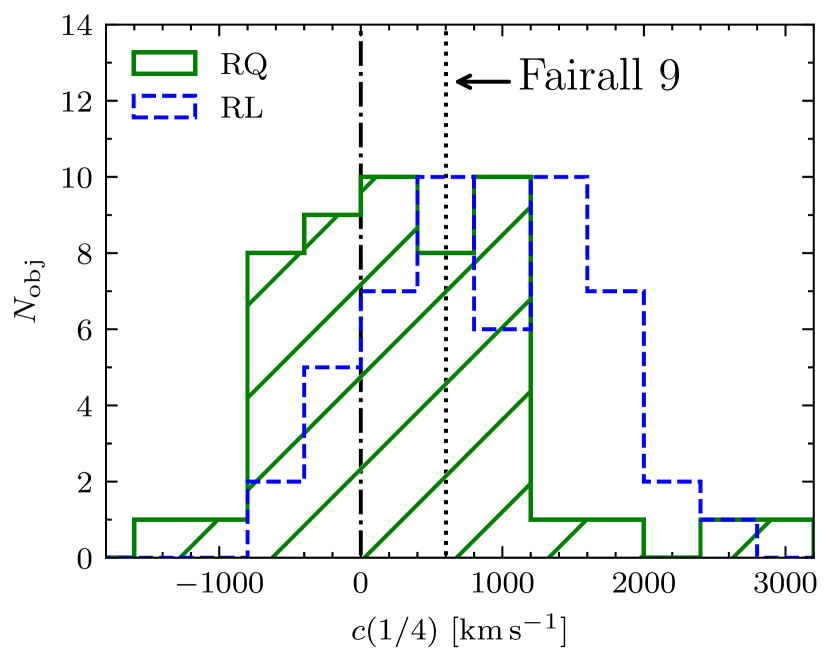
Figure 1: The measured H$\beta$ centroid at 1/4 of the maximum, based on the sample of Marziani et al. (2003a) of 101 Pop.B objects. The green histogram refers to the distribution of 51 radio-quiet (RQ) objects, while the blue histogram represents the 50 radio-loud (RL) sources. The $c(1/4)$ of Fairall 9 is $\approx 600$ $\rm km\ s^{-1}$ marked as dotted line in the plot. The 0-velocity shift is marked as dotted-dash line. The bin size is 400 $\rm km\ s^{-1}$ for both RQ and RL sources, and was set on the basis of the typical uncertainty in the $c(1/4)$ estimates.

3 Observations, Data Reduction, and Polarization Analysis

3.1 Observations

The FOcal Reducer and low dispersion Spectrograph 2 (FORS2) is installed at the Cassegrain focus of ESO’s Very Large Telescope (VLT). The spectrograph has been designed for multiple purposes in visible and near ultraviolet bands, including a polarimetric mode. The polarimetric mode allows the measurement of linear polarization. A Wollaston prism is introduced as beam splitter in the optical path, and a super-achromatic half-wave retarder plate connected to a grism with slitlets and a filter make it possible to carry out spectropolarimetry (ESO, 2019).

For our observations, we used the GRIS_300V grism and the order separation filter GG435 to fully cover the H$\beta$ and H$\alpha$ profile, and approaching a spectral resolution $\sim 800$ in the wavelength range of H$\alpha$, with a step of $\approx$ 4 Å/pix. The observation of Fairall 9 was carried out during the night of November 7, 2018, with seeing condition $\apprle 1$ arcsec. The half-wave retarder plate was rotated at angles of $0^{\circ},\ 22.5^{\circ},\ 45,\ {\rm and}\ 67.5^{\circ}$. At every individual position angle, a set of six observations was taken, each with an exposure of 240 seconds. The centroid of the target was placed in one of the Multi-Object Spectroscopy movable slitlets (MOS), with the height set to 11.4 arcseconds. The produced spectra were split into ordinary (o) and extraordinary (e) beams by the Wollaston prism, and recorded on the CCD with a separation of about 22 arcseconds (the pixel scale in the spatial direction is $D_{{\rm s}}=0.126\ {\rm arcsec\,/\,pixel}$ (ESO, 2019).

3.2 Data Reduction

We performed the standard procedure of the spectropolarimetric data reduction described in details in Afanasiev & Amirkhanyan (2012) and adopted to the VLT/FORS2 data. The reduction process includes the following steps: bias subtraction and extraction of the frames from the original fits-files, construction of the 2D model of the geometrical distortions for ordinary and extra-ordinary ray spectra, spectra linearization using He-Hg-Cd-Ar arc lamp spectrum and flat-field correction and night sky lines subtraction. The effective spectral range is 4400–7500 Å.

The o- and e-beam spectra were extracted using a fix aperture size of around 40 pixels. The size of the aperture was chosen so that the nucleus flux was totally integrated within the seeing on each exposure.

3.3 Polarization analysis

The formulæ to calculate the normalized Stokes parameters in the general form can be found in Patat & Romaniello (2006). Here we will use the relations adopted for the case of the measuring of the polarization with the Wollaston prism and rotating $\lambda$/2 plate given in Afanasiev & Amirkhanyan (2012):

$$\begin{split}Q(\lambda)&=\frac{1}{2}\left(F(\lambda)_{\theta=0^{\circ}}-F(\lambda)_{\theta=45^{\circ}}\right),\\ U(\lambda)&=\frac{1}{2}\left(F(\lambda)_{\theta=22.5^{\circ}}-F(\lambda)_{\theta=67.5^{\circ}}\right),\\ \end{split}$$ (1)

where $\theta$ is the position angle of the retarder plate and $F(\lambda)$ is the normalized flux difference between the ordinary ($f_{o}(\lambda)$) and extraordinary ($f_{e}(\lambda)$) beams:

$$F(\lambda)=\frac{f_{o}(\lambda)-f_{e}(\lambda)}{f_{o}(\lambda)+f_{e}(\lambda)}.$$ (2)

Linear polarization degree $P$ and polarization position angle are related to the Stokes parameters as:

$$\begin{split}P(\lambda)&=\sqrt{Q(\lambda)^{2}+U(\lambda)^{2}},\\ \mathrm{PA}(\lambda)&=\frac{1}{2}\arctan\frac{U(\lambda)}{Q(\lambda)}.\\ \end{split}$$ (3)

The $\pi/2$ ambiguity of the polarization angle is corrected according to the formulae given in Bagnulo et al. (2009).

Table 1: Low-polarized star properties

RA	DEC	$P$	PA	$Q$	$U$
(h:m:s)	(d:m:s)	(%)	(∘)	(%)	(%)
(1)	(2)	(3)	(4)	(5)	(6)
01:06:54.46	-59:58:01.2	0.016$\pm$0.023	110.0$\pm$35.7	-0.012$\pm$0.022	-0.010$\pm$0.021
01:31:32.58	-59:35:34.4	0.012$\pm$0.014	83.9$\pm$30.3	-0.012$\pm$0.014	0.003$\pm$0.013
01:35:14.71	-58:08:21.5	0.015$\pm$0.012	97.1$\pm$21.8	-0.015$\pm$0.012	-0.004$\pm$0.011

Notes: The three low-polarized stars from Heiles (2000). Col. (1), right ascension. Col. (2), declination. Col. (3) and (4), polarization degree($P$) and polarization position angle(PA) reported in the literature. Col. (5) and (6), the decomposed Stokes parameters $Q$ and $U$ computed from Col. (3) and (4) based on Eq. 3. All the uncertainties reported here are at $1\sigma$ confidence level

Figure 2: The change of depolarization coefficients in polarizing channels during observations for different retarder angles. The scatters are the average ratio in each frame. The dotted lines show the tendency of the ratio. Black dashed line is at the middle of observation with cross mark showing the speculative depolarization coefficients.

3.3.1 Atmospheric depolarization

The atmospheric depolarization, caused by non-selective aerosol light scattering, has a serious effect on the results of the spectropolarimetric analysis. From the data we collected, the effect could reach up to 1% (shown in Fig. 2). To eliminate such effect, we followed procedures discussed in Afanasiev & Amirkhanyan (2012). We assumed the depolarization effect is wavelength independent, and we considered the depolarization during the exposure as a variation of the spectrograph transmission for the ordinary and extraordinary rays. In this case, we used

$$F(\lambda)=\frac{D(\theta_{i})f_{o}(\lambda)-f_{e}(\lambda)}{D(\theta_{i})f_{o}(\lambda)+f_{e}(\lambda)}$$ (4)

instead of the expression in Eq. 2, where $D(\theta_{i})$ are the coefficients of the polarization transmission channels which also include the variations of the atmospheric depolarization. As it can be found in Afanasiev & Amirkhanyan (2012) these coefficients are usually obtained for each retarder position angle and for each exposure. Due to the non-optimal observational technique we had to use the time-averaged coefficients which are calculated as:

$$D(\theta_{i})=\langle{f_{\rm o}(\lambda)}/{f_{\rm e}(\lambda)}\rangle$$ (5)

where the angle brackets correspond to the averaging over the time. Correction because of atmospheric (de)polarization should be applied every time the ratio between the ordinary and extraordinary beam intensity is shown to depend on time. Even a change of $\approx$1% can yield to a large difference in the polarization angle.

3.3.2 Interstellar polarization

The interstellar matter (ISM), including molecular gas and dust, can have a considerable effect on the linear polarization because of scattering (Whittet et al., 2001). The observed polarization is a vectorial composition of the polarization of the target and ISM, and the corresponding Stokes parameters $U$ and $Q$ have the relation as:

$${(Q,U)}_{{\rm obs}}={(Q,U)}_{{\rm AGN}}+{(Q,U)}_{{\rm ISM}}$$ (6)

To determine and eliminate the ISM polarization, we used 3 low-polarized stars (Heiles, 2000) close to Fairall 9. Their polarization data are in Table 1. We assume that all 3 stars are non-polarized, and that their observed polarization is entirely caused by ISM scattering. Even assuming this one can clearly see that the polarization of the nearby stars is equal to zero within the very low errors. So, we will consider further that the interstellar polarization is negligible in the direction of Fairall 9.

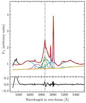
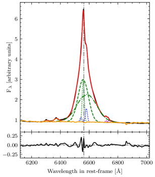
Figure 3: Decomposition of the H$\beta$ (left panels) and H$\alpha$ (right panels) natural light profiles with multiple components. The grey dot-dashed line marked the rest frame for H$\beta$ and H$\alpha$ respectively. Top-left panel: the fitting range for H$\beta$, 4430–5550 Å. The observed total flux is in solid black line while the best-fitting result is shown in red. The sum of the power-law continuum and the host galaxy component is shown as an orange line. The Fe ii blends modeled with the template are plotted in solid cyan line. Green dashed, dot-dashed and dotted lines represent the decomposed BC, VBC and NC for H$\beta$, respectively. Blue dotted lines are [O iii]$\lambda\lambda$4959, 5007. He ii$\lambda 4686$ emission are modeled with a VBC (magenta dashed line) and a NC (magenta dotted line). Dotted cyan lines stand for the high-ionization iron forbidden lines in the range 5100 – 5300 Å. Top-right panel: the fitting range for H$\alpha$, 6200–7000 Å. The black, red and orange solid lines have identical meaning as in left panel. Green dashed, dot-dashed and dotted lines represent the decomposed BC, VBC and NC for H$\alpha$, respectively. Blue dotted lines are [N ii]$\lambda\lambda$6548, 6584. Yellow dotted lines are [O i]$\lambda$6300 and [O i]$\lambda$6363. Magenta dotted lines represent [S ii]$\lambda\lambda$6717,6730. Bottom panels are the residual for the fitting with grey dashed lines marking the zero levels.

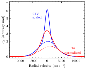
Figure 4: H$\alpha$ (red) and C iv$\lambda$1549 (blue) profiles overlaid after rescaling of C iv$\lambda$1549 to the same intensity of the H$\alpha$ red wing. H$\alpha$ and C iv$\lambda$1549 VBC are shown by dotted red and blue lines, respectively.

3.3.3 Instrumental polarization

To correct the bias of the mean level of the Stokes parameters calculating from the given spectropolarimetric data we need to correct the data for the instrumental polarization. Because no standard star of zero polarization was obtained at the night of Fairall 9 observations, the zero level of the instrumental polarization was defined from the spectra of the host-galaxy of the object. For this, we integrated the frames of the spectra in the range out of the object aperture. Assuming the instrumental polarization independent from the wavelength we obtained: $Q_{\rm ins}=0.8,\ U_{\rm ins}=-0.1$. The instrumental values were subtracted from the Stokes parameters of the object.

4 Results

4.1 Natural light decomposition

We first decomposed the H$\alpha$ and H$\beta$ emission line profile in natural light (shown in Fig. 3). A minimum-$\chi^{2}$ analysis using the IRAF task specfit (Kriss, 1994) was carried out to include all the relevant components in the H$\alpha$ spectral region from 6200 to 7000Å  with a power-law AGN continuum, host galaxy continuum, H$\alpha$ emission components, narrow forbidden lines of [O i]$\lambda$6300, [O i]$\lambda$6363, [N ii]$\lambda\lambda 6548,6584$, and [S ii]$\lambda\lambda$6717,6730. As for H$\beta$, the fitting was carried out in the spectral range from 4430 to 5550Å, including a power-law AGN continuum, host galaxy continuum, H$\beta$ emission components, the Fe ii emission blends, the narrow forbidden lines [O iii]$\lambda\lambda 4959,5007$, He ii$\lambda 4686$ emission, and Gaussians accounting for the blended emission of several high-ionization iron forbidden lines peaking at $\lambda\approx 5200$ Å  ([Fe vi]$\lambda 5146$, [Fe vii]$\lambda 5159$, [Fe vi]$\lambda 5176$, [Fe iv]$\lambda 5236$, [Fe vii]$\lambda 5276$, and [Fe xiv]$\lambda 5302$). Since the host contamination of Fairall 9 is relatively weak with respect to the active nucleus continuum, the host galaxy component in natural light has been modelled using the spectrum of the elliptical galaxy NGC 3379 (Kennicutt, 1992). The Fe ii emission templates are based on I Zw 1 from Boroson & Green (1992). The decomposition of the H$\alpha$ profile proper involved 3 Gaussians (Fig. 3): (1) the narrow component (NC), (2) the broad component (BC), (3) the very broad component (VBC) which has a substantial peak shift to the red by $\thicksim\ 1000$ $\rm km\ s^{-1}$, and accounts for the redward asymmetry of the H$\alpha$ full broad profile (i.e., BC+VBC). The decomposition of H$\beta$ also involved 3 Gaussians (see also Fig. 3): (1) one NC, (2) one BC, (3) one VBC that is shifted to the red by $\thicksim 2000$$\rm km\ s^{-1}$, leading to a more expanded red wing in the total H$\beta$ profile.

In radio-quiet Pop.B sources, C iv$\lambda 1549$ shows a systematically stronger blue side with respect to the Balmer line profiles. The excess is small and much lower than in several cases of extreme Pop. A sources that have blueshifted emission dominating the C iv$\lambda 1549$ profile (e.g., Leighly & Moore, 2004; Marinello et al., 2020, for examples). The origin of the blue excess in natural light is often considered to be due to outflowing gas, possibly in the form of a wind, dense clumps, or dense clumps embedded in a wind (see e.g. Kollatschny 2003; Proga 2003).

A HST/FOS spectrum was extracted from the MAST archive and reduced by Sulentic et al. (2007) who provide measurements of the Civ line intensity and profile parameters. The C iv $\lambda 1549$ profile of Fairall 9 has been reanalyzed in this work, with special attention to the line wings. We carried out the decomposition of the C iv $\lambda 1549$ based on HST/FOS UV spectra following the approach developed in Marziani et al. (2010). We consistently used the same components in the fitting procedure, i.e. one NC, one BC and one VBC. The result is shown in Fig. 4. Compared to H$\alpha$, C iv seems to be more symmetric, with a redshifted VBC at only a few hundred $\rm km\ s^{-1}$. This is mainly caused by two unresolved Gaussian components shifted to blue and red respectively (Marziani et al., 2010). Since the redshifted component is slightly more prominent, we can see a modest redward asymmetry in total flux. Now to help the interpretation of the H$\alpha$ profile, we superimpose and rescale the red-wing of C iv and H$\alpha$ at the same intensity (Fig. 4). Both H$\alpha$ and C iv have outstanding redward asymmetries. The red side of C iv is consistent with the one of H$\alpha$, but with a revealing difference: the centroid at 1/4 peak intensity $c(1/4)$ is 194 $\pm$199 $\rm km\ s^{-1}$ for C iv and 442$\pm$ 136 $\rm km\ s^{-1}$ for H$\alpha$, where the uncertainties are at a $2\sigma$ confidence level. If the red wings are matched, the blue side of C iv is somewhat more extended, making the C iv profile more symmetric especially close to the line base: the shift to the red of the $c(1/4)$ is only marginally significant. This implies that the C iv is affected by a small blueshifted excess, most likely associated with outflowing gas.

4.2 Polarization of the BLR

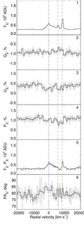
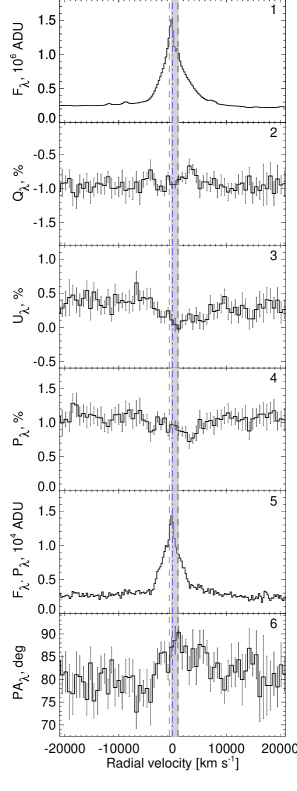
Figure 5: The profiles of H$\beta$ (left) and H$\alpha$ (right) lines. From top to bottom: the intensity in the natural light, the Q and U Stokes parameters, the polarization degree, the polarized flux and the polarization angle. The values on panels 1 and 5 are binned in 6Å window and the values on panels 2–4 and 6 – in 15Å window. The black vertical dashed lines mark the narrow lines coming from the NLR – [O iii] lines at H$\beta$ profile and [N ii] lines at H$\alpha$ profile. The blue vertical dashed line marks the position of zero velocity. For H$\alpha$  the atmospheric absorption band is noted with a light grey stripe. Error bars are at 1$\sigma$ confidence level.

After the correction for the atmospheric depolarization, ISM and instrumental polarization, we derived the polarization parameters using the method described in 3.3. The results are presented in Fig. 5.

The total intensity profiles of H$\beta$ and H$\alpha$ lines are shown in panel 1 of Fig. 5. As the contribution of the narrow lines ([O iii] and [N ii]) will depolarize the broad lines slightly but their wrong estimation will cause much larger inaccuracies, the narrow components were not subtracted from the spectra. Note here that the atmospheric absorption B-band affects the profile of H$\alpha$ line between 6860–6917 Å.

The 2nd and 3rd panels in Fig. 5 show the Stokes parameters $Q$ and $U$ binned over the 15Å-window. For each spectral bin, we estimated the robust average of the measured values over the spectral range and all taken exposures. The errors given on the plots are equal to the 1$\sigma$ level, where $\sigma$ is the robust standard deviation.

The polarization degree $P$ is plotted at the 4th panel in Fig. 5. The H$\alpha$ and H$\beta$ lines show values of the polarization percentage P% $\approx$ 0.05 % (H$\beta$) – 0.12 % (H$\alpha$) lower than the one of the average adjacent continuum polarization ($\approx 1.07$ %).

The profiles of the polarization position angle are shown on panel 5 of Fig. 5. In both the H$\beta$ and H$\alpha$ lines, one can detect a double "swing": the profiles change within around $\pm$10^∘ relatively to the mean level that the continuum polarization shows, with minimum PA around $-7000$ $\rm km\ s^{-1}$. These features point out the presence of the equatorial scattering in the nucleus region, according to Smith et al. (2005), and the detection of such profiles in both lines is a strong evidence in favor of this model. This inference is consistent with the Pop. B nature of Fairall 9 i.e., with Fairall 9 belonging to the "disk dominated" type-1 AGN (Richards et al., 2002). Following the paper by Afanasiev & Popović (2015) we examine below these profiles in details to estimate the viewing angle and the black hole mass, and to finally resolve the velocity field of the gas emitting the reflected radiation.

5 Discussion

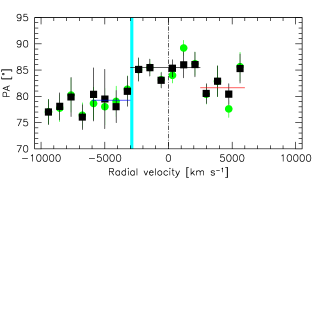
Figure 6: The PA as a function of radial velocity, for the average (black squares) and weighted average (green squares) of the H$\beta$ and H$\alpha$ PAs. Horizontal lines trace the average values of the PA over three ranges in radial velocity. The cyan stripe identifies the range over which a significant change in PA occurs, around $-2750$ $\rm km\ s^{-1}$.

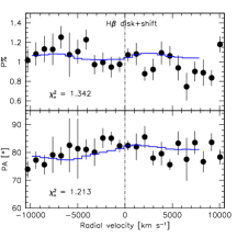
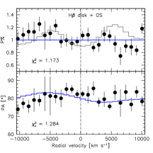
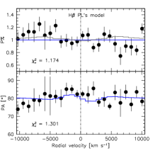
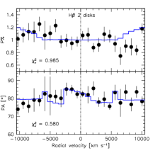
Figure 7: Comparison between several ray-tracing models and the observational data for H$\beta$. Each panel is split in half; the top one shows the polarization percentage and the bottom one the polarization PA. Top row, from left to right: results for a single disk geometry and equatorial scattering, for a single disk geometry to which an arbitrary shift has been added, and for a spherical geometry. Second row from top: biconical outflow model, disk with outflow motion of the scatterer by 500 $\rm km\ s^{-1}$, and a disk + 4000 $\rm km\ s^{-1}$ scatterer outflow, with the scatterer overlying the emission disk as developed by Lira et al. (2020). The third row are the results for a two-disk model with the two disks inclined by 30 degrees with respect to each other, with the outer disk observed at 15 degrees.

Appendix B provides stokes and skirt models for several geometric and kinematic configurations. The sketch of Fig. B.1 shows a Keplerian disk, a polar outflow region, a spherical BLR, and a double disk surrounded by the equatorial scatterer – a dusty torus. In the first part of the discussion we will describe the comparison between these and other competing models and the data, beginning with the possibility of polar scattering, while in the second part we will focus on the analysis of the models that are suggested by the data. For the quantitative $\chi^{2}$ comparison we consider only H$\beta$  up to $+5000$ $\rm km\ s^{-1}$ (beyond this radial velocity, the [Oiii] doublet destroys the polarization profile of broad H$\beta$). The H$\alpha$ profile is more heavily affected by the H$\alpha$ NC, by [N ii] emission, and by the B band within $|\delta v_{\mathrm{r}}|\lesssim 2000$ $\rm km\ s^{-1}$, right where S/N is higher. The H$\alpha$ polarization profiles gave always worse $\chi_{\nu}^{2}$ than H$\beta$, but the main features of H$\alpha$ profile are qualitatively consistent with the main features of H$\beta$. H$\alpha$ is therefore used for confirmatory purposes. The most robust, salient feature that we need to explain is the almost constant polarization degree across the H$\beta$ and H$\alpha$ profile, which in turns lead to a single-peaked polarized flux profile. The second main feature is the PA profile, whose 0 point is apparently displaced from rest frame. In this respect, Fig. 6 shows average and weighted average of the H$\beta$ and H$\alpha$ PA data. A significant change in PA is not occurring at $v_{\mathrm{r}}\approx 0$ $\rm km\ s^{-1}$, but at $v_{\mathrm{r}}\approx-2750$ $\rm km\ s^{-1}$: a Welch $t$-test yields a significance $\sim(1-3\cdot 10^{-4})$ for the change in PA between the radial velocity averages over the range $-$6000 – $-$3000 $\rm km\ s^{-1}$and $-$3000 – $+$2500 $\rm km\ s^{-1}$ (blue and black lines in Fig. 6). The absence of a “swing" centered at $v_{\mathrm{r}}\approx 0$ $\rm km\ s^{-1}$ is also visible in Figs. 5 and Fig. A.2 for both H$\beta$ and H$\alpha$, and their average is reinforcing the result at a statistical level.

5.1 Polar scattering

In the previous discussion we have assumed that the scattering region is equatorial, with relatively small inclination with respect to the symmetry plane offered by the accretion disk. However, this assumption may not be fully adequate. For Pop. B sources like Fairall 9, the inclination is relatively large. It is reasonable to consider the effect of polar scattering as done by Smith et al. (2004). In the interpretation of Smith et al. (2004) of sources showing evidence of both polar and equatorial scattering, the polar scattering region is subdivided into (1) a scattering cone aligned with the emission disk axis, but with a very large opening angle as shown in Fig. 10 of Smith et al. (2004); (2) a spherical wedge at large inclination (but still low enough for the line of sight not to intercept the torus). If the main component of the polar scatterer is distributed in this configuration, we can expect that the width of the polarized flux feature and of the swing PA pattern will be narrowed, polarization degree lowered, and that PA might be different in the continuum and in the line.

A combination of polar and equatorial scattering appears, in principle a possibility. This would not have been a first occurrence by far. A combination of polar and equatorial scattering is expected as a general feature of type-1, where the polar scattering electrons are provided by gas in correspondence of the narrow-line region (Smith et al., 2004). This could make it possible to form a central peak in the polarization profile. The inclination estimates imply that the line of sight may pass close to the edge of the torus. However, Fairall 9 is a very low polarization object, with no sign of significant reddening and highly polarized continuum, suggesting that it should be seen well above the torus (and with the line of sight not passing through the wedge). The source is different from Fairall 51, the prototypical “Seyfert on the edge.” In addition, if a polar scatterer is assumed as in region (1) of Smith et al. (2004), we should see evidence of narrowing in the polarized flux feature and in the swing PA pattern, which we don’t: the swing PA pattern is wide.

5.2 Model inter-comparison

Fig. 7 shows the data superimposed to the best fits from the models discussed below. The minimum normalized $\chi_{\nu}^{2}$ values obtained from the model best fits to the data are reported in each panel. The continuum polarization has been added and the polarization % predicted by the model has been scaled by a free factor to obtain a minimum $\chi^{2}$. They are computed in the range $-10000\leq v_{\mathrm{r}}\leq 6000$ $\rm km\ s^{-1}$. Beyond 6000 $\rm km\ s^{-1}$, there is evidence of depolarization associated with the narrow [O iii] emission. Considering that the number of degrees of freedom is $16$, for most models, an F-test based on the normalized $\chi_{\nu}^{2}$ ratios for the different models would require a minimum $F(1,2)=\chi_{\nu,1}^{2}/\chi_{\nu,2}^{2}\approx 1.268$ for detecting a difference that is significant at a 1$\sigma$ confidence level. The minimum $\chi_{\nu}^{2}$ is often consistent with a flat or almost flat behavior, which might imply a very low polarization degree associated with a low optical depth of the scatterer. To show the behavior expected for each model, the grey histogram line in Fig. 7 traces the model predictions in an arbitrary scale.

5.2.1 Single disk model + equatorial scatterer

Having excluded polar scattering, we turn to the Keplerian disk and equatorial scatterer model that we implicitly applied for the $M_{\rm BH}$ estimate. This is the model that has been successfully applied to several tens of type-1 AGN (Afanasiev et al., 2019). It shows a typical double-swing feature of PA with the $\mathrm{PA}_{\mathrm{max}}$ amplitude decreasing as the viewing inclination increases. The polarized line is broader than the line in natural light and the degree of polarization shows double-peaked profiles with maxima in the wings and minimum in the core (Fig. B.2). However, the polarized flux profile of Fairall 9 is single peaked for both H$\beta$ and H$\alpha$. The polarization percentage across the profiles changes little, and may indicate a different situation from the simple case of the rotational motion in a flat disk and equatorial scatter. Fig. 7 shows that the agreement between data and model is fair. The $\chi^{2}$ is not very high for both the polarization % and the polarization PA. The single disk profile seen at an inclination of $\approx 30$ degrees is consistent with the data for both the P% and the PA, supporting the presence of rotational motions.

No improvement is obtained if a blueshift of about $\approx 2500$ $\rm km\ s^{-1}$ is imposed to the disk model. This ad hoc modification is suggested by the PA profile that is not symmetric around 0, as already shown in Fig. A.2. A shift would significantly lower the H$\alpha$ PA $\chi^{2}$. However, for H$\alpha$ the improvement in the polarization angle is not accompanied by a corresponding agreement in the polarization % profile, and for H$\beta$ there is no significant improvement.

5.2.2 Spherical BLR

The spherical BLR model involves an isotropic velocity dispersion along with the spherical geometry. The typical double-swing feature of PA is visible also in this case, and the models of the single Keplerian disk and the spherical BLR give similar results. The agreement is again fair. A shift to the blue by $\approx-2000$$\rm km\ s^{-1}$ improves the polarization % profile, at the expense of a worsening of the PA $\chi_{\nu}^{2}$.

5.2.3 Outflows

We considered a model for which the BLR geometry follows a bi-conic outflow with constant velocity(Fig.  B.1, top second panel, Zheng et al., 1990; Marziani et al., 1996; Corbett et al., 2000). Such model produces a clear double-peaked unpolarized lines, while the polarized line is highly asymmetric with blue part being dominant towards intermediate viewing angles, while the red part is dominant towards pole-on view. The Stokes parameter $U$ is anti-symmetric with respect to the line center, while $Q$ is asymmetric, which results in asymmetric double-swing PA profiles. The biconic model provides the minimum $\chi_{\nu}^{2}$ among all models, but the fit of the PA profile is poor, and disfavored at a 1$\sigma$ confidence level. Biconical outflows require high Eddington ratio and may therefore be specific of sources accreting at higher rate than Fairall 9.

Pop. B sources also show evidence of outflows as discussed in Section 4, even if less powerful than in Pop. A. We consider two alternatives. The first, outflow in the scattering medium located at the inner edge of the torus (in the previous models the scatterer was assumed stationary) yields a poor $\chi^{2}$. As in the case of the single disk, the model predicts two peaks in the % of polarization that are not observed. The model with an outflowing scatterer overlying the disk emission could be interpreted as a disk wind, perhaps driven by magneto-hydrodynamical forces (Emmering et al., 1992). Unlike the cases studied by Lira et al. (2020), the agreement with our data is not good: the $\chi_{\nu}^{2}$ of the P% profile is consistent with unity (even if the minimum $\chi_{\nu}^{2}$ obtained for a flat profile), but the PA profile is not favored.

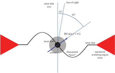
Figure 8: Sketch (not drawn to scale; the curvature of “bowl” is greatly exaggerated, and there should be no discontinuity between the outer and inner disk, see Fig. 9) illustrating the warped disk geometry suggested in this paper.

5.2.4 Double Keplerian disk

We simplified the warped disk with a combination of two disk-like BLRs at two inclinations (the two-disk model): the inner disk corresponding to region (2) is rotated by an angle of $30^{\circ}$ around the $x$-axis with inner and outer radius of 1000 $r_{\rm g}$ to 2000 $r_{\rm g}$. The outer disk (region 1) is situated in the asymptotic plane that contains the equatorial plane of the torus (Fig. 8) and extends from 2000 $r_{\rm g}$ to 10000 $r_{\rm g}$. Region 3 is represented as the point-like source of the continuum. The models of Fig. 3 provide qualitative confirmation of the feature seen in the Fairall 9 spectrum. Fig. 7 shows the polarization parameters predicted for two inclined disk configuration (third row from top). It is interesting to note that the inclination of the inner disk of the model (45^∘) is consistent with the angle estimated by Lohfink et al. (2012) using X-ray spectra($\sim 48^{\circ}$). The warp geometry might imply that the innermost disk emitting the X-continuum and the inner disk in the model may be facing each other (Fig. 8).

The main features observed in the polarization profile of Fairall 9 are recognizable in the models.

1. The polarized flux in Fig. 5 shows a centrally peaked structure. The two-disk models shown in the Figs. B.3 and B.2 of Appendix B show the sum of two concentric “rings” and clearly represent an oversimplification with respect to the reality of a warped disk. A real warped disk can be assimilated to a sequence of narrow rings with inclination progressively closer to the one of the Kerr black hole equatorial plane, easily producing a single peaked polarization profile. The point here is that a flat polarization percentage profile within $\pm 5000$ $\rm km\ s^{-1}$  yields a polarized flux profile that is centrally peaked as the profile in natural light (panels 5 of Fig. 5). This behavior is qualitatively consistent with the polarized flux profile expected for a warped disk, and is not consistent with the one expected from a single rotating disk and an equatorial stationary scatterer.

2. Negative $\Delta\mathrm{PA}$ in the radial velocity range from -10000 to -3000 $\rm km\ s^{-1}$ are predicted by models and are qualitatively consistent with the change observed in the data (bottom panel of Fig. 5).

3. The shape of the PA around 0 $\rm km\ s^{-1}$ is predicted by the model if the disk at $\phi\approx 0^{\circ}-45^{\circ}$, Fig. 7 can also explain the observed PA shape that suggests a change in the sign in the polarization angle at non-zero radial velocities.

Fig. 7 shows the model overlaid to the data point. The $\chi_{\nu}^{2}$ is the lowest among the different model, and best agreement is obtained for the azimuthal angle $\phi=15^{\circ}$ case. A $\chi_{\nu}^{2}\approx 0.99$ is obtained for the P% of the 2 disk model. It is just a factor 1.15 larger than the $\chi_{\nu}^{2}$ obtained for the biconic model and, according to the $F$-test criterion, not significantly different. The PA profile of the two-disk model has a significantly lower $\chi_{\nu}^{2}$ with respect to all other cases, at least by a factor $\gtrsim 2$, implying that the difference is significant at a confidence level of more than $1\sigma$, and close to 90%.

The innermost part of the BLR is expected to be seen at inclination $\gtrsim 30^{\circ}$ (and significantly different from the 10 – 15 degrees inferred for the outer disk), because of the relatively modest $\Delta\mathrm{PA}$ in the swing that implies relatively high values of the viewing angle. A warp can indeed change the viewing angle of the line emitting region in the innermost part of the BLR, lowering the swing amplitude. Fig. B.2 shows that the amplitude of the swing is decreasing with viewing angle (Smith et al., 2005). If these effects are taken into account, the $M_{\rm BH}$ derived from spectropolarimetry might be underestimated.

However, the polarized flux predictions consistent with a warped disk and the agreement with the two-disk model PA profile suggest that a two-disk system or a warped disk might be the most appropriate models.

5.3 A transient second disk

The model that produces best agreement with the data involves two disks at different inclinations with respect to the line of sight. A tidal disruption event (TDE) could have given rise to a second accretion disk. Fairall 9 has been described as a changing look AGN in recent papers. It has passed from a very low state in the early 1980s (Kollatschny & Fricke, 1985); however, in the low state the broad lines almost never disappeared. Although TDEs are relatively short lived, and destined to fade in the course of a few years, there are claims of longer events (Lin et al., 2017). In the case of Fairall 9, the $V$ observations of the ASAS-SN (Shappee et al., 2014) indicate remarkable photometric stability over the period May 2014 – Sept. 2018, with an average $V\approx 13.77$ mag and a dispersion of just $\approx 0.07$ mag. We suggest that the strong change occurred in the 1980s might be a “long-term event of sustained accretion" (Trakhtenbrot et al., 2019). These events might be typical of AGN, and especially among Pop. B sources accreting at relatively low rates.

5.4 A warped disk

Apart from a second disk due to a TDE, the only mechanism known to us that may yield a change in disk orientation on the spatial scale of the inner BLR is Lense-Thirring precession, produced by the misalignment between the spin of the black hole and the angular momentum vector of the accreting gas (Bardeen & Petterson, 1975).

The expectations for a warped structure involve three main regions: (1) an outer, asymptotic disk with a well-defined tilt angle of the plane of the disk relative to the equatorial plane of the black hole $\beta_{0}$; (2) an intermediate region where inclination $\beta$ can be much larger than $\beta_{0}$; (3) a region within $\lesssim 100$ gravitational radii where the disk is in the equatorial plane of the rotating black hole. The third region is probably too hot to account for the observed emission line spectrum. It is more likely to host the X-ray corona (Begelman et al., 1983; Haardt & Maraschi, 1993; Różańska & Czerny, 2000), and be the source of most UV and X continuum. See Fig. 8 for a schematic representation of a warped structure tentatively adjusted to the observational constraints on Fairall 9.

Modeling the exact geometry of a warped disk is difficult since three Euler angles are needed to define the orientation of a warped structure in space. In the warped disk scenario, the inflection on the natural line profile of H$\alpha$ roughly separates two regions: the outer one (region 1), Keplerian, still in the plane of the accreting gas, and an innermost one more inclined, exposed to the full strength of the AGN continuum, and producing the high-ionization VBC (region 2; the illuminated “bowl” of Fig. 8; see Bachev (1999) for a computation of the detailed illumination and self-shadowing patterns in a warped disk geometry). Assuming $M_{\rm BH}$ $\approx 2\cdot 10^{8}$ $\rm M_{\rm\astrosun}$, the radial BLR distance measured from reverberation mapping corresponds to $\approx 1700r_{\mathrm{g}}$. A change of inclination can be induced, on a spatial scale of $\sim 10^{3}r_{\mathrm{g}}$ by Lense-Thirring precession (Bardeen & Petterson, 1975).

The trends of Fig. 9 represent the behavior of the inclination angle of the warped disk $\beta$ as a function of the radial distance in units of gravitational radii for $J=0.1,0.5,1$, and are expected for Lense-Thirring precession as computed by Bardeen & Petterson (1975). The Lense-Thirring scale is consistent with the linear scale derived from $r_{\mathrm{BLR}}$. It is also interesting to see that we expect a strong increase in the inclination of the disk at a few hundred gravitational radii from the black hole, and that inclination of the disk start deviating from the one of the equatorial plane of the black hole at smaller distances for lower $J$. This is in turn expected to increase the direct illumination of the disk by the central UV/X continuum source, known to be very low in the case of a geometrically thin disk (see e.g., Section 5.10 of Frank et al., 2002).

The gravitational + transverse redshift in the VBC goes as $\delta z\approx\frac{3}{2}r_{\mathrm{g}}/r$ (Bon et al., 2015). Therefore, the VBC emission could be strongly affected by gravitational redshift: the rotational velocity scales with $r^{-\frac{1}{2}}$, implying that $r\approx(c/v)^{2}r_{\mathrm{g}}$. For a rotational velocity $v\sim 15000$ $\rm km\ s^{-1}$, $r\approx 450r_{\mathrm{g}}$, and we obtain a gravitational + transverse redshift $\sim 1000$ $\rm km\ s^{-1}$. Fig. 9 shows that the $\beta$ value remains close to 0 up 400 $r_{\mathrm{g}}$ for the case of a maximally rotating black hole ($J\approx 0.994$, Thorne, 1974). If $J<1$, as mentioned, the maximum radius at which the disk plane lies in the equatorial plane of the black hole should be lower. Therefore, gas at very small radii could be more efficiently illuminated, and the emitted radiation should be even more strongly affected by gravitational redshift with $J<1$ than with $J\approx 1$.  A Suzaku measurement of the Fairall 9 spin yields $J\approx 0.60\pm 0.07$ (Schmoll et al., 2009).

A Kerr black hole is in principle capable of producing a rotation of the polarization plane via the “gravitational Faraday effect” (Ishihara et al., 1988). The effect is achromatic, but strongly dependent on the distance from the central black hole: the rotation $\delta\mathrm{PA}\approx\frac{5}{4}\pi mJ\cos\theta_{0}/r^{3}_{\mathrm{min}}$, where $m$ is the mass of the black hole in the natural units, $r_{\mathrm{min}}$ is a photon impact parameter, and $\theta_{0}$ is the angle between the spin of the black hole and the line-of-sight. Assuming $r\sim 100m$, $J\sim 1$, $\cos\theta_{0}\sim 1$, the $\delta\mathrm{PA}\ll 1$ degree. Even if recent numerical simulations suggest a larger effect (Chen et al., 2015), a significant $\delta\mathrm{PA}$ ($\sim$ 10 degrees) is possible only at $r\lesssim 10r_{\mathrm{g}}$, i.e., for photons in the X-ray domain.

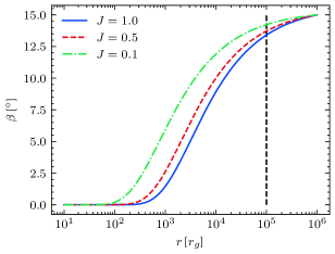
Figure 9: The solution of Eq. (9) in Bardeen & Petterson (1975) with different angular momentum J in units of $M_{\rm BH}$². The tilt angle $\beta$ is normalized to 15^∘ at $10^{6}r_{\rm g}$. Other parameters in the equation are set to unity.

Invoking a warped disk presents several drawbacks. Warps are expected to be rare, as they require special conditions: rejuvenation of a black hole from gas whose angular momentum is not aligned with black hole spin. Large systematic redshifts and blueshifts should be equally possible (Wang & Li, 2012), as the illuminated bowl of a warped disk would lose axial symmetries (Bachev, 1999). The large shifts and irregular profiles predicted by kinematical models are relatively rare (but large blueshifts are found; see several examples in Zamfir et al. (2010), while the Balmer line profiles of Fairall 9 are fairly typical for a Pop. B object). However, the redward asymmetry might be always associated with gravitational redshift (see in this respect Popović et al., 1995; Corbin, 1995), and a warped geometry may contribute to make it more evident, as the bowl shape should make it possible to efficiently expose the line emitting gas at a few hundreds gravitational radii.

5.4.1 Fairall 9: analogies and differences with E 1821+643 and Mark 668

The broad emission Balmer lines of E 1821+643 show an unusual shape with a highly red asymmetric profile and a large broad line peak redshifted ($\sim$ 1000 $\rm km\ s^{-1}$) relative to the narrow lines (see Shapovalova et al., 2016). However, E 1821+643 is a striking example of profile reversal in polarized light, where to a prominent redward asymmetry corresponds a prominent blueshifted excess in polarized light (Smith et al., 2002) explained by the emission of one active component of a binary super-massive BH or a recoiling black hole after collision (Robinson et al., 2010). As done by Robinson et al. (2010), we identify two components in the BLR, one with 0 or a smaller redshift, and one broader with a larger redshift ($\sim 2000$ $\rm km\ s^{-1}$). However, considering that the features can be identified in most Pop. B sources (about 50 % of quasars), it seems unlikely that they could be due to a bulk motion of the BLR with respect to the host galaxy. Since the broader feature is ascribed to the inner most part of the emitting regions, profile reversal in natural light (i.e., the redward asymmetry turning into a blue one or profile turning from asymmetric to symmetric or vice-versa) should be expected on timescales of a few years. The first published spectrum of sufficient quality was obtained in 1977 (Hawley & Phillips, 1978); the H$\beta$ profile is remarkably similar to the one of the observations in 2019. Over a 42 yr time lapse the total displacement is significantly larger than the BLR distance from the central continuum source: $\approx 2.65\cdot 10^{17}$ cm, assuming a constant velocity of 2000 $\rm km\ s^{-1}$. If the original BLR radius was $\approx 1.44\cdot 10^{17}$ cm, the recoiling displacement added to the original radius implies that the ionization parameter of the gas “left behind” in the BLR should be lower by a factor $0.1$, and that there should have been a decrease in the H$\alpha$ and H$\beta$ BC intensity with respect to the VBC by a factor $\approx 0.38$, assuming the same, typical conditions for the BLR. There is no positive evidence of this decrease (for an account of the variability pattern, see Lub & de Ruiter (1992)). Kollatschny & Fricke (1985) reported the almost disappearance of the broad H$\beta$ emission between 1981 and 1983, but afterwards the AGN bounced back to its pre-1981 spectrum. Further monitoring on a timescale of a decade should provide a stringent test on the recoiling black hole hypothesis.

Mrk 668 (OQ 208) is known since long because of a redshifted peak by $\sim 2600$ $\rm km\ s^{-1}$  in the natural light profile of H$\beta$ (Gezari et al., 2007, and references therein). The peak radial velocity has remained approximately constant since the first report on the shifted feature, over 40 years ago (Osterbrock & Cohen, 1979). In this case, the presence of a black hole binary is not supported by the data (Doan et al., 2020). The spectropolarimetric data are consistent with $b=-0.5$ suggesting a predominance of Keplerian motion. The $\Delta\mathrm{PA}$ changes sign at $\delta v_{\mathrm{r}}\thicksim 0$, as in the case of Fairall 9 (Afanasiev et al., 2019).

A warped disk geometry is affected by self shadowing, as the disk illumination is strongly dependent on the azimuthal angle $\phi$. Single peaks highly displaced to both the red and blue are predicted for the Balmer line profiles in natural light (Bachev, 1999; Wu et al., 2008). In the case of Mrk 668, optical Fe ii emission shows a consistent shift with the Balmer lines (Bon et al., 2018), providing additional evidence supporting that we are seeing low-ionization emission lines from a virialized, Keplerian system, with the Fe ii emission occurring predominately at the outer edge of the disk, as expected (Panda et al., 2020, and references therein). On the ground of the stability of the profile over a timescale longer than the dynamical timescale of the BLR, and of its spectropolarimetric properties, we suggest that OQ 208 could be considered as a warped disk candidate.

5.5 $M_{\rm BH}$ and $L_{\rm Bol}/L_{\rm Edd}$ estimate for Fairall 9

5.5.1 $M_{\rm BH}$

The details of the $M_{\rm BH}$ computations following the spectropolarimetric and other methods are reported in Appendix A. The various estimates reported in Table 3 disagree by a factor almost $3$, within the range $M_{\rm BH}$$\approx(1.2-3.3)\cdot 10^{8}$ $\rm M_{\rm\astrosun}$. Each method has some strong point but also some difficulties. The spectropolarimetric mass estimate depends on the distance of the scatterer, which in turns depends on scaling laws connecting it to luminosity (Tab. 3). The weighted average of the $M_{\rm BH}$ values reported in Table 3 from spectropolarimetry is $M_{\rm BH}\approx(1.49\pm 0.48)\cdot 10^{8}$ $\rm M_{\rm\astrosun}$. It is doubtful whether the Afanasiev et al. (2019) method can be applied in warped disk geometry. Indeed, the uncertainty in the $a$ parameter rather large, $\delta a\approx 0.13$ and $\approx 0.15$ for H$\beta$ and H$\alpha$, respectively, if compared to the typical uncertainties reported by Afanasiev et al. (2019), always $\lesssim 0.12$. However, the spectropolarimetric estimate compares well with the average from the application of the virial relation using $r_{\mathrm{BLR}}$ from reverberation mapping, as reported in Table 3, even if it is significantly lower than the estimate obtained from 2 scaling laws based on the H$\alpha$ FWHM, and especially from the width of the Si absorption line at 1.59 $\mu$m, which indicate $M_{\rm BH}\gtrsim 2\cdot 10^{8}$ M_⊙. We computed a median and weighted average black hole mass considering all methods (even if they are not fully independent). The median $M_{\rm BH}\approx(1.68\pm 0.48)\cdot 10^{8}$ $\rm M_{\rm\astrosun}$ (with the semi-interquartile range as uncertainty) and the weighted average $M_{\rm BH}\approx(1.71\pm 0.63)\cdot 10^{8}$ $\rm M_{\rm\astrosun}$ are both consistent with the $M_{\rm BH}$ derived from spectropolarimetry, and also with the previous determination of Recondo-Gonzalez et al. (1997).

The Pop. B $M_{\rm BH}$ distribution at low-$z$ covers the black hole mass range $8\lesssim\log$$M_{\rm BH}$$\lesssim 10$ [$\rm M_{\rm\astrosun}$], in flux-limited samples built on long-slit or fiber optical spectroscopic observations (Shen et al., 2011; Marziani et al., 2003b). This result would place Fairall 9 toward the low end of the $M_{\rm BH}$ distribution for Pop. B. However, these samples are subject to a strong selection bias, as sources with a relatively small black hole mass ($M_{\rm BH}$$\sim 10^{6}$ M_⊙) radiating at low Eddington ratio are increasingly lost even at modest redshift. Very recently, the MANGA survey (Yan et al., 2016) has made it possible to detect low-luminosity, type-1 AGN associated with black hole mass even in the intermediate $M_{\rm BH}$ domain (Mezcua & Domínguez Sánchez, 2020, Hernandez-Toledo et al. 2021, in preparation). The loss of Pop. B sources is also relevant at high redshift, as the flux limit of large surveys introduces an Eddington ratio-dependent cut-off at any given $M_{\rm BH}$ (Sulentic et al., 2014).

5.5.2 $L_{\rm Bol}/L_{\rm Edd}$ 

The bolometric luminosity of Fairall 9 has been estimated as $L_{\rm Bol}\sim 4.75\cdot 10^{45}$ erg s^-1 by integrating the observed SED. The SED for Fairall 9 is provided by Brown et al. (2019), which includes photometric and spectroscopic observations of the AGN ranging from $2.5\cdot 10^{-5}$ to $9.6\cdot 10^{2}$ $\rm{\mu}$m. The Eddington luminosity can be written as $L_{\mathrm{Edd}}=1.5\cdot 10^{38}({M_{\rm BH}}/{M_{\odot}})$ erg s^-1. For $M_{\rm BH}$$\approx 2\cdot 10^{8}$ $\rm M_{\rm\astrosun}$, the Eddington ratio is $L_{\rm Bol}/L_{\mathrm{Edd}}\sim 0.16$, consistent with Pop. B but close to the limit. The observations of Brown et al. (2019) refer to a period when the source was in a high state; assuming the flux of Bentz et al. (2009) (also consistent with the average of the Santos-Lleó et al. 1997 monitoring campaign) corrected for the host galaxy contribution would imply a bolometric luminosity $L_{\rm Bol}\sim 1.65\cdot 10^{45}$ erg s^-1, and an Eddington ratio $\approx 0.06$. The variability notwithstanding, Fairall 9 has remained within the limit of Eddington ratio associated with Pop. B ($\approx 0.2$).

6 Conclusion

Using VLT/FORS2 we obtained spectropolarimetric observations of the radio-quiet Pop.B source Fairall 9. The measured polarization properties have been used for inferring constraints on the kinematics and geometry of the BLR as well as on the scattering region. Our results on the spectropolarimetric properties of Fairall 9 can be summarized as follows.

1. Fairall 9 shows low degree of polarization in correspondence of the Balmer H$\beta$ and H$\alpha$ emission lines. The polarized flux profiles of both lines are centrally peaked.

2. The polarization angle in the center of H$\beta$ and H$\alpha$ is atypical, in the sense that the "swing" shape is not as regular as the one seen in most cases by Afanasiev et al. (2019), and the dynamical center may be shifted with respect to rest frame.

3. We consider several scenarios from the Monte Carlo, ray-tracing code STOKES and SKIRT: disk-like BLR, bipolar outflowing BLR, spherical BLR, and two-disk BLR. The minimum $\chi^{2}$ in $\Delta\mathrm{PA}$ is obtained for the two-disk case.

4. The agreement with the two-disk hypothesis indicates that the inner disk may be tilted with respect to the outer disk, and that emission from the VBC may be associated with the inner disk.

5. The possibility of a second disk originating from a tidal-disruption event is not favored on the ground of the photometric behavior of Fairall 9 right in the four years preceding the spectropolarimetric observations.

6. Excluding the possibility of a TDE-produced disk, the most likely hypothesis appears to be a warped structure driven by Lense-Thirring precession. Models support the possibility that a double disk structure may be at the origin of the PA, polarized flux, and polarization percentage behavior.

7. Using the width of the polarized broad H$\beta$ and H$\alpha$ profile, we estimated the inclination and the central black hole mass. The inclination effect plays a significant role in the emission line broadening especially in Pop. B sources. For Fairall 9, the inclination angle cannot be determined as easily as for other sources, but is constrained around $50^{\circ}$. The corresponding virial factor is $\approx 2$. The derived values are consistent with the expected role of the viewing angle along the FWHM axis in the optical plane of the E1 MS (Marziani et al., 2001; Panda et al., 2019). However, if a warped structure is present, then to consider a single value of the viewing angle could be misleading.

8. The central black hole mass obtained by using the spectropolarimetric method of Afanasiev et al. (2014) is somewhat lower with respect to the mass estimates from most other methods, which give an average $M_{\rm BH}$ $\sim 2\times 10^{8}$$\rm M_{\rm\astrosun}$. However, The slope $b$ is consistent with the value expected for predominance of a Keplerian velocity field.

If our inferences are correct, the case of Fairall 9 confirms the dominance of Keplerian motions in the BLR of Pop. B sources. The issue of orientation is complicated by the warped structure revealed in this source. The results on Fairall 9 further strengthen the hypothesis that gravitational redshift might be the governing factor of the VBC redshift, due to the easy illumination of the disk gas in a warped geometry (in this respect, Punsly et al. (2020) suggest that at very low $L_{\rm Bol}/L_{\rm Edd}$, the effect of gravitational redshift is strong because only the innermost part of the disk is illuminated by the AGN continuum). Deep, high-resolution observations of other Pop. B sources are however needed to test whether the spectropolarimetric results obtained for Fairall 9 may be common and general.

Data availability

The data underlying this article will be shared on reasonable request to the corresponding author.

Appendix A The estimated black hole mass

A.1 The inclination effect

In optical spectroscopy, we can observe only the line-of-sight velocity distribution of the BLR. Therefore, it is obvious that inclination of the BLR will play a significant role in the line width (Collin et al., 2006). Spectropolarimetry is a powerful tool to eliminate the inclination effect, since the intrinsic Keplerian velocity distribution can be obtained from the polarized profiles. The effect of inclination can be quantified by assuming that the line broadening is due to an isotropic component plus a flattened component, whose velocity field projection along the line of sight is $\propto 1/\sin i$, where $i$ is the inclination of the system to the line of sight. Thus, the observed velocity distribution is:

$$\delta v_{obs}^{2}=\frac{1}{3}\delta v_{{\rm iso}}^{2}+\delta v_{{\rm K}}^{2}\sin^{2}i$$ (7)

where $\delta v_{{\rm iso}}$ is an isotropic component, $\delta v_{{\rm K}}$ is the Keplerian velocity, and their ratio should be $\kappa=\delta v_{{\rm iso}}/\delta v_{{\rm k}}\gtrapprox 0.1$ (Collin et al., 2006; Marziani et al., 2018). In our work, we use the lower limitation of the ratio, i.e. $\kappa=0.1$, and the $\delta v_{{\rm obs}}$ is the FWHM of the observed line profile from single epoch observations, i.e. $\delta v_{{\rm obs}}={\rm FWHM}_{\rm obs}$.

Then the virial factor which relates black hole mass $M_{\rm BH}$ can be written as:

$$M_{{\rm BH}}=f_{\rm FWHM}\frac{R_{{\rm BLR}}}{G}{\rm FWHM_{\rm obs}^{2}}$$ (8)

where $G$ is the gravitational constant, $R_{\rm BLR}$ is the radius of the BLR. $M_{\rm BH}$ is also related to the Keplerian velocity ${\rm FWHM}_{\rm k}$ as:

$$M_{{\rm BH}}=\frac{R_{{\rm BLR}}}{G}{{\rm FWHM}_{\rm k}^{2}}$$ (9)

Therefore the virial factor can be written as:

$$f_{\rm FWHM}=\frac{{{\rm FWHM}_{\rm k}^{2}}}{{\rm FWHM_{\rm obs}^{2}}}=\left[\frac{1}{3}\kappa^{2}+\sin^{2}i\right]^{-1}$$ (10)

In the Fairall 9 case, the possible concurrence of a more complex geometry such as disk warping makes the interpretation of the width of the polarization profile uncertain. In order to measure the velocity dispersion associated with the Keplerian motion, we applied the decomposition technique (as mentioned before) to the H$\beta$ and H$\alpha$ polarized flux (Fig. A.1). To estimate $f$, here we consider two different velocity FWHM of the H$\beta$ and H$\alpha$ profile in natural light: one associated with BC only and one with BC+VBC. The corresponding inclinations and virial factors are reported in Table 2. The BC FWHM is the parameter expected to be more strongly affected by orientation, and the $f$ value derived for H$\beta$ BC is the one used for the $M_{\rm BH}$ computation.

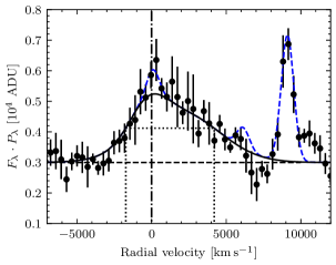
Figure A.1: Top panel: black dots with error-bars at 1$\sigma$ confidential level represent the polarized flux for H$\beta$. Black solid line shows the best fitting for the total broad polarized profile with two Gaussian components, with dotted lines showing the FWHM. Blue dashed lines represent the narrow polarized components. The continuum level is plotted in black dashed line. The zero radial velocity is marked with dot-dashed line. Bottom panel: same as top panel except for H$\alpha$ polarized profile.

Table 2: Inclination and virial factor estimation

Line component	FWHM($F_{\lambda}$)	FWHM($P_{\lambda}\cdot F_{\lambda}$)	$i$	$f$
	($\rm km\ s^{-1}$)	($\rm km\ s^{-1}$)	(∘)
(1)	(2)	(3)	(4)	(5)
H$\beta$ BC	4010	5925	42.4	2.18
H$\beta$ BC+VBC	5307	5925	63.3	1.25
H$\alpha$ BC	3848	5107	48.7	1.76
H$\alpha$ BC+VBC	5050	5107	80.8	1.02

Notes: Col. (1), emission line and components in natural light used for the inclination and virial factor estimation. Col. (2), FHWM of the components in natural light. Col. (3), FWHM of the total broad profile in polarized light. Col. (4) and (5), inclination and corresponding virial factor estimated with Eq. 10, respectively.

A.1.1 Spectropolarimetric method

Several methods are being presently used to estimate the central black hole mass, starting from Eq. 8. We consider first the spectropolarimetric data that can be used to estimate the black hole mass from the “mark” of Keplerian motion on PA, in a way that is independent from the viewing angle (see Afanasiev & Popović, 2015, for a detailed description of the method). In short, a rotating Keplerian BLR will produce a polarized light by equatorial scattering, where the PA of the polarization changes in a way that is correlated to the velocity field of the BLR. The relation between the velocity and the PA is (Afanasiev & Popović, 2015; Afanasiev et al., 2019):

$$\log(\frac{V_{i}}{c})=a-0.5\log(\tan(\Delta\mathrm{PA}_{i}))$$ (11)

where $c$ is the speed of light, and the $\Delta\mathrm{PA}_{\mathrm{i}}$ are the ones of Fig. A.2. The slope is set to 0.5 to be consistent with the assumption of Keplerian motion within the BLR. The intercept $a$ is a function of $M_{\rm BH}$ and can be written as

$$a=0.5\log(\frac{GM_{{\rm BH}}\cos^{2}(\theta)}{c^{2}R_{{\rm sc}}})$$ (12)

where $G$ is the gravitational constant, $R_{\rm sc}$ is the inner radius of the scattering region, and $\theta$ is the angle between the BLR and the scatterer plane. Based on our assumption of equatorial scattering, $\theta$ should be very close to 0. However, it is worth noting that a non-coplanar torus has $\theta\sim 10-20^{\circ}$, and thus may introduce a systematic underestimate on $M_{\rm BH}$ at $\sim 10\%$ (Afanasiev & Popović, 2015).

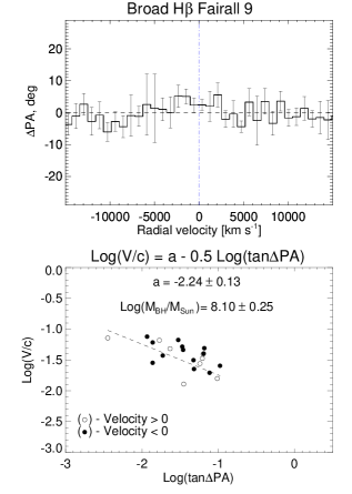
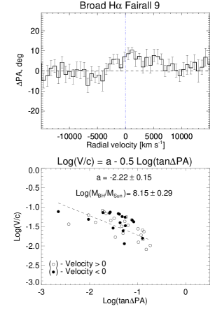
Figure A.2: The polarization angle profiles for H$\beta$ (left) and H$\alpha$ (right) lines. On the upper panels the deviation of the polarization angle to the mean value (horizontal dashed line) is given. The maximum $\Delta\mathrm{PA}$ is 6^∘ for H$\beta$ and 10^∘ for H$\alpha$. The vertical dashed lines mark the center of the emission lines. The grey shaded area show the contamination of the [O iii] emission for H$\beta$ and the atmospheric B band absorption for H$\alpha$ respectively. The bottom panels show the relation of $\log(v_{\mathrm{r}}/c)$ v.s. $\log(\tan\Delta\mathrm{PA})$. The $M_{\rm BH}$ shown here is estimated assuming $R_{\rm sc}=215$ light days.

First, we verified that the slope is indeed consistent with a Keplerian velocity field. A bisector fit yields $b\approx-0.492\pm 0.065$, consistent with the expected value $b=-0.5$. We then determined $a$ by fitting the velocity and PA by linear regression (shown in Fig. A.2). The estimated value is $a=-2.24\pm 0.13$ for H$\beta$ and $-2.22\pm 0.15$ for H$\alpha$  (with uncertainties at 1$\sigma$ confidence level). To estimate the inner radius of the scattering region, we apply two techniques. First, we consider the dust lag-luminosity correlation described in Koshida et al. (2014) that yields the following relation between the time lag in K band (days) and the luminosity in V band:

$$\log\text{$\Delta$}t_{\rm K}=a_{{\rm s}}+b_{\rm s}M_{{\rm V}}$$ (13)

where $a_{\rm s}=-2.11\pm 0.04.$ and $b_{\rm s}=-0.2$, both given by Koshida et al. (2014). Fairall 9 is known as variable source (Santos-Lleó et al., 1997), with secular trends superimposed to shorter time scale variation of a significant amplitude. We consider here the $V\approx$13.36 for the nucleus of Fairall 9 provided by Griersmith & Visvanathan (1979), at an epoch when the AGN was reputed to be in a ”bright” phase. The corresponding $V$ absolute magnitude is $M_{\rm V}=-23.0$, after applying a correction because of Galactic extinction ($A_{\mathrm{V}}\approx 0.071$). Here we assume that the time lag reflects the inner radius of the scattering region, i.e. $R_{{\rm sc}}=c\Delta t_{K}\approx 310$ light days. Using Eq. 12 we can estimate the black hole mass, which is shown in Table 4(a).

The radius of the scattering region $R_{\mathrm{sc}}$ can also be estimated following Afanasiev et al. (2019) who define a relation between FUV observations and $R_{\mathrm{sc}}$ from GALEX observations. The specific at 1516 Å for a 7 arcsec aperture is $\approx 3.08$ mJy. Trouble is, the FUV flux of Fairall 9 is strongly variable. The IUE average flux obtained during the reverberation mapping campaign of Fairall 9 by Rodriguez-Pascual et al. (1997) are consistent with the GALEX values, but the rms is $\approx$ 30%, with the source doubling in flux on a timescale of 6 month. Applying the relation of Afanasiev et al. (2019) after extinction correction, we obtain $R_{\mathrm{sc}}\approx 215$ ld. This second $M_{\rm BH}$ estimate is also reported on Table 4(a).

A.1.2 Other methods

The RM method

The RM method is based on the response of the broad emission lines to the continuum variations. Reliable estimates of the lag between the continuum and the H$\beta$ broad emission line light curves for over 100 AGNs are presently available (Du & Wang, 2019, and references therein). The rest-frame time lag in H$\beta$ obtained using cross-correlation function (CCF) by Peterson et al. (2004) is $\tau=17.4_{-4.3}^{+3.2}$ days. Alternatively, the rest-frame lag can be derived with a statistical technique called JAVELIN (Zu et al., 2011, formerly known as SPEAR). RM provides the line emitting region radius that can be entered in Eq. 8. The measured line width for the full H$\beta$ profile is $\rm FWHM(\rm H\beta)=4010\pm 18$ $\rm km\ s^{-1}$. The H$\beta$ lines has been studied in the past as the major virial broadening estimator for $M_{\rm BH}$ computation. In order to compute $M_{\rm BH}$, we use velocity dispersion measures for the BC with corresponding virial factors, and with time lag obtained using different techniques. The final results for $M_{\rm BH}$ are reported in Table 4(b).

The AGN Black Hole Mass Database (Bentz & Katz, 2015) reports the values of radii and line width measurements on the rms specta from the optical and UV reverberation mapping campaigns (Santos-Lleó et al., 1997; Rodriguez-Pascual et al., 1997). The last entry in Table 4(b) refer to the H$\beta$ rms dispersion $\sigma$, with a $f\approx 3.76$.

The R-L scaling relations

The RM observations of more than 70 AGNs so far have led to an empirical correlation between radius of the BLR and the luminosity of the continuum, i.e. the R-L relation (Kaspi et al., 2000; Bentz et al., 2009). This relation has made possible single-epoch $M_{\rm BH}$ estimations for large samples of quasars: $M_{\rm BH}$ is derived just from the continuum (or emission line) luminosity and line width of single-epoch spectroscopy (Vestergaard, 2002; Vestergaard & Peterson, 2006; Greene & Ho, 2005). In Table 4(c), the luminosity of the continuum at 5100 Å is obtained from Bentz et al. (2009), which already has the host contamination subtracted. The nucleus luminosity of H$\beta$ BC is derived from Marziani et al. (2003a), and the luminosity of H$\alpha$ is converted from $L_{5100}$ using the empirical relation given by Greene & Ho (2005).

The $M_{\mathrm{BH}}-\sigma_{\star}$ relation

The $M_{\rm BH}$ and the stellar velocity dispersion ($\sigma_{\star}$) in the host galaxy bulge has been found to be strongly correlated (Ferrarese & Merritt, 2000; Gebhardt et al., 2000; Nelson, 2000). However, for luminous Seyfert 1 galaxies like Fairall 9 it is relatively difficult to detect the virial motion in the host galaxy. Nelson & Whittle (1996) have found a strong correlation between $\sigma_{\star}$ and the FWHM of [O III]$\lambda 5007$ for the majority of Seyfert galaxies, indicating that the [O III]$\lambda 5007$ profile is dominated by virial motion in the bulge potential. Therefore we use $\sigma_{\star}={\rm FWHM}_{\rm[O{\sc III}]}/2.35$ where ${\rm FWHM}_{\rm[O{\sc III}]}=425$ $\rm km\ s^{-1}$  is measured by Whittle (1992) with the instrumental effects corrected. The only direct stellar velocity dispersion measurement we are aware of: Oliva et al. (1995) found $228\pm 20$ $\rm km\ s^{-1}$ from the mid-IR feature of Si at $1.59\mu$m. The values are consistent but the IR value needs to be carefully calibrated, as a small difference can yield to a large mass difference. In order to determine the correlation between $M_{\rm BH}$ and $\sigma_{\star}$, previous work carried out by McConnell et al. (2011) separated the entire sample of 65 local galaxies into two sub-samples (early type and late type) based on their morphology. We report in Table 4(d) the $M_{\rm BH}$ estimates based on the early-type, late-type and entire sample scaling laws of McConnell et al. (2011), although the scaling law derived for the entire sample should be preferred because of a better statistics.

Table 3: $M_{\rm BH}$ Estimates

Line	$M_{V}$1	$L_{\mathrm{GALEX}}(1516)$	$R_{\rm sc}$	$a$	$\cos{\theta}$	$M_{\rm BH}$	Notes/Refs.
	(mag)	($\rm{{10^{44}\,erg\,s^{-1}}}$)	(ld)			($10^{7}M_{{\rm\astrosun}}$)
(1)	(2)	(3)	(4)	(5)	(6)	(7)	(8)
H$\beta$	…	2.75	$215$	$-2.24\pm 0.13$	$\sim 1$	$12.5\pm 7.5$	Afanasiev et al. (2019); Feigelson & Babu (1992)
H$\beta$	-23.0	…	$310$	$-2.24\pm 0.13$	$\sim 1$	$18.2\pm 10.8$	Afanasiev & Popović (2015); Koshida et al. (2014)
H$\alpha$	…	2.75	$215$	$-2.22\pm 0.15$	$\sim 1$	$13.7\pm 9.5$	Afanasiev et al. (2019); Feigelson & Babu (1992)
H$\alpha$	-23.0	…	$310$	$-2.22\pm 0.15$	$\sim 1$	$19.8\pm 13.6$	Afanasiev & Popović (2015); Koshida et al. (2014)

(a) Spectropolarimetry

Notes: $M_{\rm BH}$ estimated with spectropolarimetric data using Eq. 12. Col. (1), emission line for mass estimation. Col. (2), absolute magnitude in $V$ band transformed from the nuclear apparent magnitude measured by Griersmith & Visvanathan (1979). Col. (3), GALEX luminosity at 1516Å. Col. (4), radius of the scattering region estimated with Eq. 13(second and fourth rows) or Afanasiev et al. (2019) method (first and third rows). Col. (5), intercept of the linear regression as shown Fig. A.2. Col. (6), cosine of the angle $\theta$ between BLR plane and the inner scattering region, which is assumed to be close to 1($\theta\sim 0$). Col. (7), the estimated black hole mass with uncertainties at 1$\sigma$ confidential level. Col. (8), references for the apparent magnitude, GALEX luminosity, and their relation with $R_{\rm sc}$.

Line component	$f$	$R_{{\rm BLR}}$	FWHM	$M_{\rm BH}$	Lag technique	Lag Ref
		(light days)	(${\rm km\,s^{-1}}$)	$(10^{7}M_{{\rm\astrosun}})$
(1)	(2)	(3)	(4)	(5)	(6)	(7)
H$\beta$ BC	2.18	$17.4^{+3.2}_{-4.3}$	$4010\pm 18$	$11.9^{+2.2}_{-2.9}$	CCF	Peterson et al. (2004)
H$\beta$ BC	2.18	$19.4^{+42.1}_{-3.8}$	$4010\pm 18$	$13.3^{+28.8}_{-2.6}$	JAVELIN	Zu et al. (2011)
H$\beta$ rms $\sigma^{\dagger}$	3.76	$17.4^{+3.2}_{-4.3}$	$3787\pm 197$	$18.3^{+3.9}_{-4.9}$	CCF	Peterson et al. (2004)

(b) Virial - $r_{\mathrm{BLR}}$ from H$\beta$ RM

Notes: ^†As reported in the AGN Black Hole Mass Database (Bentz & Katz, 2015).

Col. (1), emission line and component. Col. (2), virial factor for corresponding line component(see Table 2. Col. (3), radius of the BLR obtained using different techniques. Col. (4), FWHM for different lines. The value for H$\alpha$ has been rescaled to the correlating H$\beta$ width. Col. (5), black hole mass estimated with Eq. 8. Col. (6), techniques for obtaining the time lags. Col. (7), references for the lags.

Relation	FWHM	$L$	$M_{\rm BH}$	Relation Ref
	($\rm km\ s^{-1}$)	($\rm{{10^{44}\,erg\,s^{-1}}}$)	$(10^{7}M_{{\rm\astrosun}})$
(1)	(2)	(3)	(4)	(5)
FWHMHβ, $L_{5100}$	$4010\pm 18$	$1.38\pm 0.08$	$15.4\pm 0.8$	Vestergaard & Peterson (2006)
FWHMHα, $L_{5100}$	$3847.8\pm 9.6$	$1.38\pm 0.08$	$24.1\pm 1.4$	Bentz et al. (2009); Assef et al. (2011)
FWHMHα, $L_{\rm H\alpha}$	$3847.8\pm 9.6$	$0.15\pm 0.01$	$31.7\pm 6.5$	Greene & Ho (2005); Shen et al. (2011)

(c) Scaling laws

Notes: single epoch $M_{\rm BH}$ estimated with scaling relations. Col. (1), empirical relations between the emission line FWHM and the luminosity. Col. (2), emission line FWHM. Col. (3), luminosity of the continuum or emission line. Col. (4), the estimated $M_{\rm BH}$. Col. (5), references for the luminosity and the scaling relation.

Samples	$\sigma_{\star}$	Line	$M_{\rm BH}$	$\sigma_{\star}$ Ref
	($\rm km\ s^{-1}$)		($10^{7}$$\rm M_{\rm\astrosun}$)
(1)	(2)	(3)	(4)	(5)
entire	$215\pm 20$	Si(1.59$\mu$m)	$28.2\pm 15.5$	Oliva et al. (1995)
entire	$181\pm 10$	[O iii]$\lambda 5007$	$11.7\pm 3.7$	Whittle (1992)
early type	$215\pm 20$	Si(1.59$\mu$m)	$33.3\pm 16.1$	Oliva et al. (1995)
early type	$181\pm 10$	[O iii]$\lambda 5007$	$15.2\pm 4.4$	Whittle (1992)

(d) $M_{\rm BH}$$-\sigma_{\star}$ correlation

Notes: $M_{\rm BH}$ estimated with the empirical $M_{\rm BH}$$-\sigma_{\star}$ correlation. The empirical $M_{\rm BH}$$-\sigma_{\star}$ correlation of McConnell et al. (2011) is provided for three different samples analyzed in their work. Col. (1), samples for regression in McConnell et al. (2011). Col. (2), stellar dispersion. Col. (3), emission/absorption line for stellar dispersion estimation. Col. (4), the estimated $M_{\rm BH}$. Col. (5), references of the emission/absorption line dispersion.

Appendix B Polarization modeling

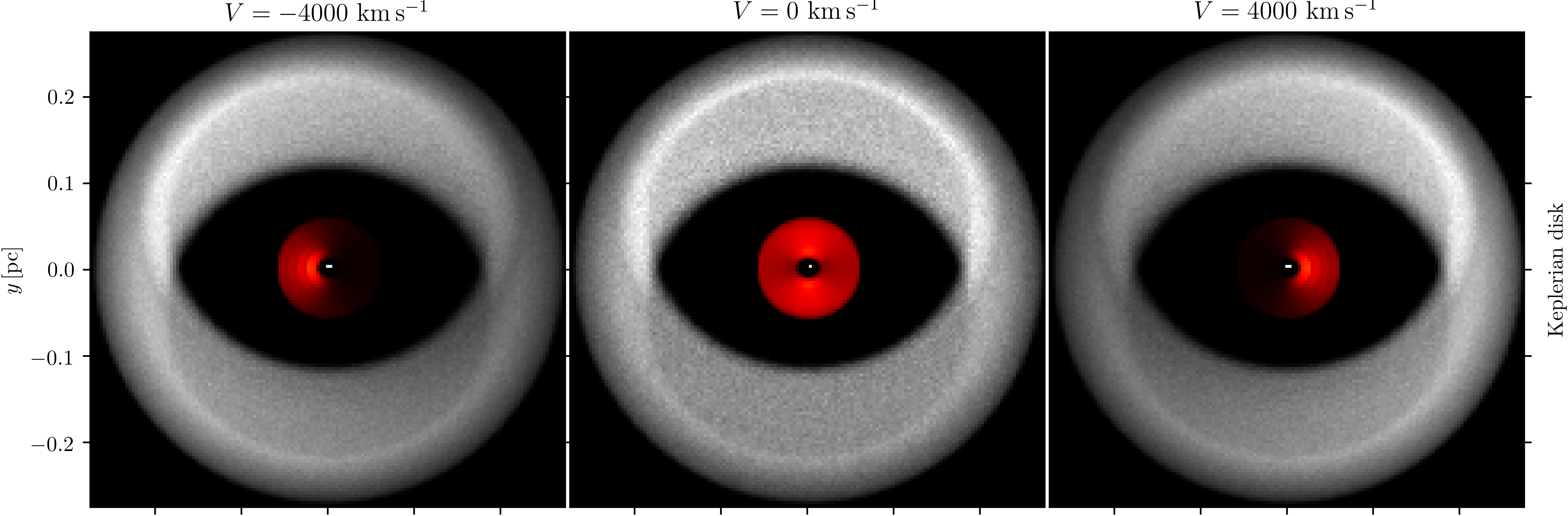
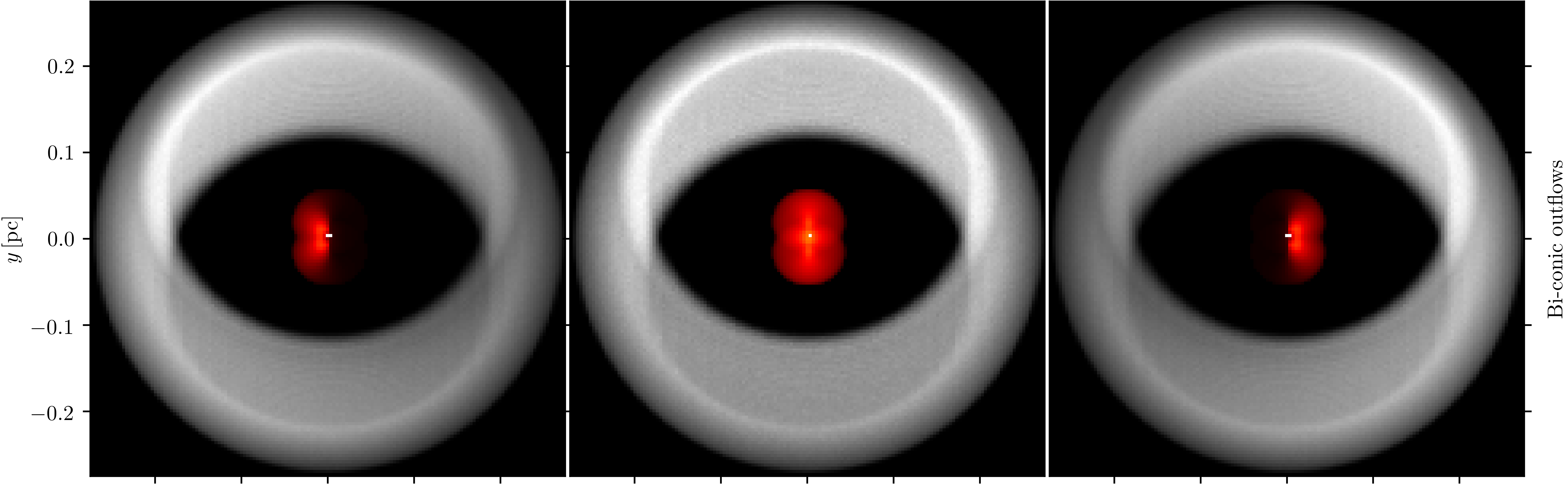
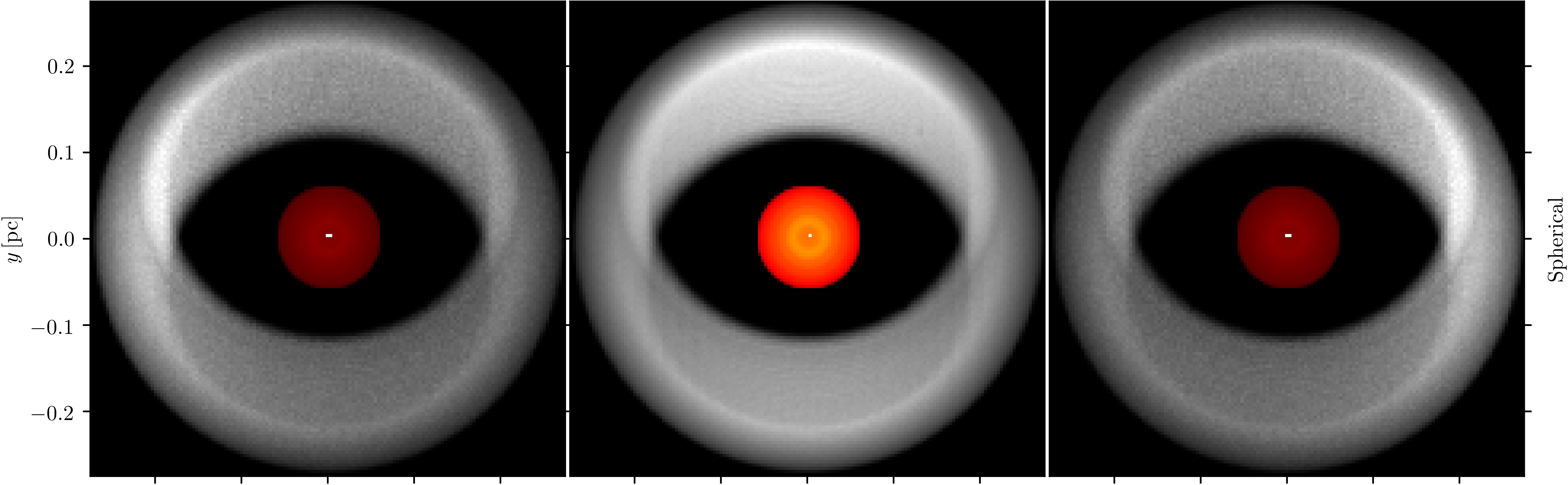
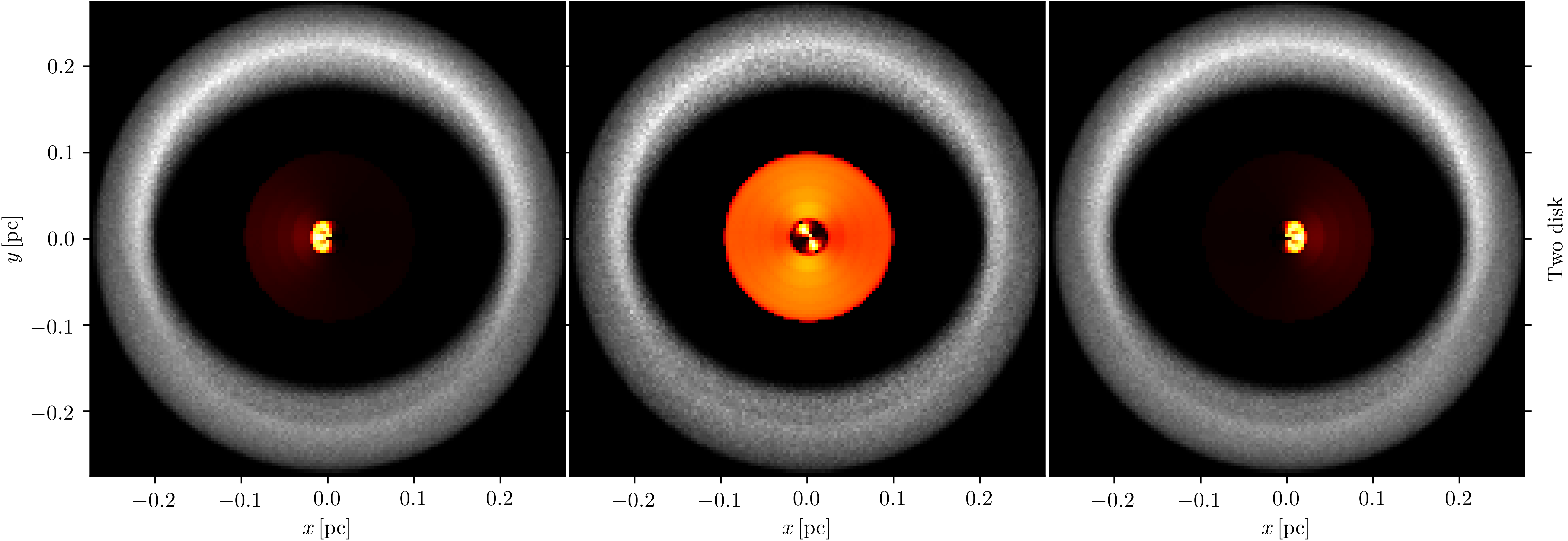
Figure B.1: Geometric setup of our models. BLR geometry from top to bottom: Keplerian disk, double-cone, spherical and two disk model. From left to right: radiation emitted at V = -4000, 0 and 4000 $\rm km\ s^{-1}$. The scattering region is shown in gray. The point source approximates the accretion disk emission. All the models except the two disk model are viewed at an inclination of $25^{\circ}$. The two disk model is viewed at an inclination of the outer disk $15^{\circ}$ and azimuth $\phi=45^{\circ}$.

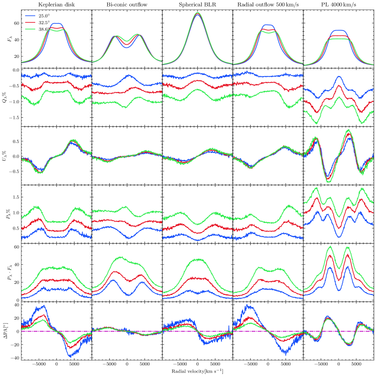
Figure B.2: Polarization parameters for three of the models (Keplerian disk, biconical outflow, and spherical BLR) considered in this work, at three different inclination values: total unpolarized flux (top row), polarized flux (second from top), Stokes parameters $Q_{\lambda}$ and $U_{\lambda}$, degree of linear polarization $P_{\lambda}$ (second row from bottom), polarization position angle(bottom).

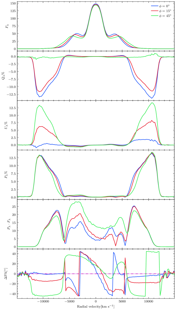
Figure B.3: Same as Fig.  B.2, but for the two disk model. The system is viewed at inclination $i=15^{\circ}$ and azimuth $\phi=0^{\circ},\,15^{\circ}$and $45^{\circ}$ (blue, red and green lines respectively).

In order to investigate various effects of different BLR geometry and kinematics on the polarization spectra, we performed three simulations using radiative transfer codes stokes (Goosmann & Gaskell, 2007; Marin et al., 2012; Marin et al., 2015; Rojas Lobos et al., 2018; Marin, 2018) and skirt (Baes et al., 2019; Camps & Baes, 2020, and references therein). We assumed that the BLR emission is being scattered by the inner part of the dusty torus. We assumed three different geometries of the BLR: disk-like, bi-conic and spherical (Fig.  B.1).

The velocity field for each BLR geometry was chosen respectively as Keplerian, radial outflows and random motion. The inner radius of the BLR was taken from the RM measurements as the mean value: $R_{\mathrm{in}}^{\mathrm{BLR}}=18\,\mathrm{ld}$. The BLR outer radius was calculated based on bolometric luminosity $R_{\mathrm{out}}^{\mathrm{BLR}}=0.2L_{46}^{0.5}\,\mathrm{pc}=70\,\mathrm{ld}$ (Laor & Draine, 1993). The bolometric luminosity was calculated from optical luminosity $L_{5100}$ (Runnoe et al., 2012). The inner radius of the scattering region $R_{\mathrm{in}}^{\mathrm{SR}}=262\,\mathrm{ld}$ was estimated from the UV $L_{\textsc{galex}}(1516)$ (Afanasiev et al., 2019). The outer radius of the SR was taken as the distance in the equatorial plane from which the half-opening angle of the outer edge of the BLR is viewed at the angle of $25^{\circ}$, i.e. $R_{\mathrm{out}}^{\mathrm{SR}}=R_{\mathrm{out}}^{\mathrm{BLR}}/\sin 12.5^{\circ}=322\,\mathrm{ld}$ (same as it was done by Savić et al., 2018). The total radial depth of the SR is set to unity. The SMBH mass was set to $M_{\mathrm{BH}}=2\times 10^{8}\,M_{\odot}$. All parameters of the model using the mean value of each observable given in Table 3. For every simulation, we used one BLR configuration while keeping the same SR. Each of the BLR configuration has the same inner and outer radius.

In Fig.  B.2 (due to azimuthal symmetry), we show the profiles of the total unpolarized flux (top panels), polarized flux $p\times F$ (top second panels), Stokes parameters $Q$ (top third panel), $U$ (top fourth panels), the degree of linear polarization $p$ (top fifth panels) and PA(bottom panels) for the disk-like, bi-conic and spherical BLR geometry (from left to right respectively).

A warped disk was modeled as two disks: the inner and the outer. The inner disk was set from 1000 $r_{\rm g}$ to 2000 $r_{\rm g}$ and rotated along the $x-$axis for $30^{\circ}$. The outer disk continues from 2000 $r_{\rm g}$ up to 10000 $r_{\rm g}$ Fig.  B.1 (bottom panels). The system is viewed at an inclination $i=15^{\circ}$ and at azimuthal angles $\phi=0^{\circ},\,\,22.5^{\circ}\,\,45^{\circ}$ and $90^{\circ}$. Polarization profiles for the two disk model is shown in Fig.  B.3.

References

- Afanasiev & Amirkhanyan (2012) Afanasiev V. L., Amirkhanyan V. R., 2012, Astrophysical Bulletin, 67, 438
- Afanasiev & Popović (2015) Afanasiev V. L., Popović L. Č., 2015, ApJ, 800, L35
- Afanasiev et al. (2014) Afanasiev V. L., Popović L. Č., Shapovalova A. I., Borisov N. V., Ilić D., 2014, MNRAS, 440, 519
- Afanasiev et al. (2019) Afanasiev V. L., Popović L. Č., Shapovalova A. I., 2019, MNRAS, 482, 4985
- Assef et al. (2011) Assef R. J., et al., 2011, ApJ, 742, 93
- Bachev (1999) Bachev R., 1999, A&A, 348, 71
- Baes et al. (2019) Baes M., Peest C., Camps P., Siebenmorgen R., 2019, A&A, 630, A61
- Bagnulo et al. (2009) Bagnulo S., Landolfi M., Landstreet J. D., Land i Degl’Innocenti E., Fossati L., Sterzik M., 2009, PASP, 121, 993
- Baldi et al. (2016) Baldi R. D., Capetti A., Robinson A., Laor A., Behar E., 2016, MNRAS, 458, L69
- Bardeen & Petterson (1975) Bardeen J. M., Petterson J. A., 1975, ApJ, 195, L65
- Begelman et al. (1983) Begelman M. C., McKee C. F., Shields G. A., 1983, ApJ, 271, 70
- Bentz & Katz (2015) Bentz M. C., Katz S., 2015, PASP, 127, 67
- Bentz et al. (2009) Bentz M. C., Peterson B. M., Netzer H., Pogge R. W., Vestergaard M., 2009, ApJ, 697, 160
- Bon et al. (2015) Bon N., Bon E., Marziani P., Jovanović P., 2015, Ap&SS, 360, 7
- Bon et al. (2018) Bon E., Marziani P., Berton M., Bon N., Antonucci R., Gaskell M., Ferland G., 2018, in Revisiting Narrow-Line Seyfert 1 Galaxies and their Place in the Universe. p. 7 (arXiv:1812.05828)
- Boroson & Green (1992) Boroson T. A., Green R. F., 1992, ApJS, 80, 109
- Brotherton et al. (1994) Brotherton M. S., Wills B. J., Francis P. J., Steidel C. C., 1994, ApJ, 430, 495
- Brown et al. (2019) Brown M. J. I., Duncan K. J., Landt H., Kirk M., Ricci C., Kamraj N., Salvato M., Ananna T., 2019, MNRAS, 489, 3351
- Camps & Baes (2020) Camps P., Baes M., 2020, Astronomy and Computing, 31, 100381
- Chen et al. (2015) Chen B., Kantowski R., Dai X., Baron E., Maddumage P., 2015, ApJS, 218, 4
- Collin et al. (2006) Collin S., Kawaguchi T., Peterson B. M., Vestergaard M., 2006, A&A, 456, 75
- Corbett et al. (2000) Corbett E. A., Robinson A., Axon D. J., Young S., 2000, MNRAS, 319, 685
- Corbin (1995) Corbin M. R., 1995, ApJ, 447, 496
- Czerny & Hryniewicz (2011) Czerny B., Hryniewicz K., 2011, A&A, 525, L8
- Dalla Bontà et al. (2020) Dalla Bontà E., et al., 2020, arXiv e-prints, p. arXiv:2007.02963
- Decarli et al. (2011) Decarli R., Dotti M., Treves A., 2011, MNRAS, 413, 39
- Doan et al. (2020) Doan A., Eracleous M., Runnoe J. C., Liu J., Mathes G., Flohic H. M. L. G., 2020, MNRAS, 491, 1104
- Du & Wang (2019) Du P., Wang J.-M., 2019, ApJ, 886, 42
- ESO (2019) ESO 2019, Very Large Telescope Paranal Science Operations FORS2 User Manual. VLT-MAN-ESO-13100-1543, European Southern Observatory, 105 edn
- Emmanoulopoulos et al. (2011) Emmanoulopoulos D., Papadakis I. E., McHardy I. M., Nicastro F., Bianchi S., Arévalo P., 2011, MNRAS, 415, 1895
- Emmering et al. (1992) Emmering R. T., Blandford R. D., Shlosman I., 1992, ApJ, 385, 460
- Fairall (1977) Fairall A. P., 1977, MNRAS, 180, 391
- Feigelson & Babu (1992) Feigelson E. D., Babu G. J., 1992, ApJ, 397, 55
- Ferrarese & Merritt (2000) Ferrarese L., Merritt D., 2000, ApJ, 539, L9
- Fraix-Burnet et al. (2017) Fraix-Burnet D., Marziani P., D’Onofrio M., Dultzin D., 2017, Frontiers in Astronomy and Space Sciences, 4, 1
- Frank et al. (2002) Frank J., King A., Raine D. J., 2002, Accretion Power in Astrophysics: Third Edition, iii edition edn. Cambridge University Press, Cambridge
- Gebhardt et al. (2000) Gebhardt K., et al., 2000, ApJ, 539, L13
- Gezari et al. (2007) Gezari S., Halpern J. P., Eracleous M., 2007, ApJS, 169, 167
- Goosmann & Gaskell (2007) Goosmann R. W., Gaskell C. M., 2007, A&A, 465, 129
- Greene & Ho (2005) Greene J. E., Ho L. C., 2005, ApJ, 630, 122
- Griersmith & Visvanathan (1979) Griersmith D., Visvanathan N., 1979, A&A, 79, 329
- Haardt & Maraschi (1993) Haardt F., Maraschi L., 1993, ApJ, 413, 507
- Hawley & Phillips (1978) Hawley S. A., Phillips M. M., 1978, ApJ, 225, 780
- Heiles (2000) Heiles C., 2000, AJ, 119, 923
- Ishihara et al. (1988) Ishihara H., Takahashi M., Tomimatsu A., 1988, Phys. Rev. D, 38, 472
- Jarvis & McLure (2006) Jarvis M. J., McLure R. J., 2006, MNRAS, 369, 182
- Kaspi et al. (2000) Kaspi S., Smith P. S., Netzer H., Maoz D., Jannuzi B. T., Giveon U., 2000, ApJ, 533, 631
- Kennicutt (1992) Kennicutt Robert C. J., 1992, ApJS, 79, 255
- Kollatschny (2003) Kollatschny W., 2003, A&A, 407, 461
- Kollatschny & Fricke (1985) Kollatschny W., Fricke K. J., 1985, A&A, 146, L11
- Kormendy & Ho (2013) Kormendy J., Ho L. C., 2013, ARA&A, 51, 511
- Kormendy & Richstone (1995) Kormendy J., Richstone D., 1995, ARA&A, 33, 581
- Koshida et al. (2014) Koshida S., et al., 2014, ApJ, 788, 159
- Kriss (1994) Kriss G., 1994, Astronomical Data Analysis Software and Systems III, A.S.P. Conference Series, 61, 437
- Kuraszkiewicz et al. (2004) Kuraszkiewicz J. K., Green P. J., Crenshaw D. M., Dunn J., Forster K., Vestergaard M., Aldcroft T. L., 2004, ApJS, 150, 165
- Laor & Draine (1993) Laor A., Draine B. T., 1993, ApJ, 402, 441
- Leighly & Moore (2004) Leighly K. M., Moore J. R., 2004, ApJ, 611, 107
- Lin et al. (2017) Lin D., et al., 2017, Nature Astronomy, 1, 0033
- Lira et al. (2020) Lira P., Goosmann R. W., Kishimoto M., Cartier R., 2020, MNRAS, 491, 1
- Lohfink et al. (2012) Lohfink A. M., Reynolds C. S., Miller J. M., Brenneman L. W., Mushotzky R. F., Nowak M. A., Fabian A. C., 2012, ApJ, 758, 67
- Lohfink et al. (2016) Lohfink A. M., et al., 2016, ApJ, 821, 11
- Loveday (1996) Loveday J., 1996, MNRAS, 278, 1025
- Lub & de Ruiter (1992) Lub J., de Ruiter H. R., 1992, A&A, 256, 33
- Marin (2018) Marin F., 2018, A&A, 615, A171
- Marin et al. (2012) Marin F., Goosmann R. W., Gaskell C. M., Porquet D., Dovčiak M., 2012, A&A, 548, A121
- Marin et al. (2015) Marin F., Goosmann R. W., Gaskell C. M., 2015, A&A, 577, A66
- Marinello et al. (2020) Marinello M., Rodríguez-Ardila A., Marziani P., Sigut A., Pradhan A., 2020, MNRAS,
- Marziani & Sulentic (2012) Marziani P., Sulentic J. W., 2012, NARev, 56, 49
- Marziani et al. (1996) Marziani P., Sulentic J. W., Dultzin-Hacyan D., Calvani M., Moles M., 1996, ApJS, 104, 37
- Marziani et al. (2001) Marziani P., Sulentic J. W., Zwitter T., Dultzin-Hacyan D., Calvani M., 2001, ApJ, 558, 553
- Marziani et al. (2003a) Marziani P., Sulentic J. W., Zamanov R., Calvani M., Dultzin-Hacyan D., Bachev R., Zwitter T., 2003a, ApJS, 145, 199
- Marziani et al. (2003b) Marziani P., Zamanov R. K., Sulentic J. W., Calvani M., 2003b, MNRAS, 345, 1133
- Marziani et al. (2010) Marziani P., Sulentic J. W., Negrete C. A., Dultzin D., Zamfir S., Bachev R., 2010, MNRAS, 409, 1033
- Marziani et al. (2018) Marziani P., et al., 2018, Frontiers in Astronomy and Space Sciences, 5, 6
- Marziani et al. (2019) Marziani P., et al., 2019, A&A, 627, A88
- Mauch et al. (2003) Mauch T., Murphy T., Buttery H. J., Curran J., Hunstead R. W., Piestrzynski B., Robertson J. G., Sadler E. M., 2003, MNRAS, 342, 1117
- McConnell et al. (2011) McConnell N. J., Ma C.-P., Gebhardt K., Wright S. A., Murphy J. D., Lauer T. R., Graham J. R., Richstone D. O., 2011, Nature, 480, 215
- Mejía-Restrepo et al. (2018) Mejía-Restrepo J. E., Lira P., Netzer H., Trakhtenbrot B., Capellupo D. M., 2018, Nature Astronomy, 2, 63
- Mezcua & Domínguez Sánchez (2020) Mezcua M., Domínguez Sánchez H., 2020, ApJ, 898, L30
- Nelson (2000) Nelson C. H., 2000, ApJ, 544, L91
- Nelson & Whittle (1996) Nelson C. H., Whittle M., 1996, ApJ, 465, 96
- Oliva et al. (1995) Oliva E., Origlia L., Kotilainen J. K., Moorwood A. F. M., 1995, A&A, 301, 55
- Osterbrock & Cohen (1979) Osterbrock D. E., Cohen R., 1979, MNRAS, 187, 61
- Panda et al. (2018) Panda S., Czerny B., Adhikari T. P., Hryniewicz K., Wildy C., Kuraszkiewicz J., Śniegowska M., 2018, The Astrophysical Journal, 866, 115
- Panda et al. (2019) Panda S., Marziani P., Czerny B., 2019, arXiv e-prints, p. arXiv:1905.01729
- Panda et al. (2020) Panda S., Martínez-Aldama M. L., Marinello M., Czerny B., Marziani P., Dultzin D., 2020, arXiv e-prints, p. arXiv:2004.05201
- Patat & Romaniello (2006) Patat F., Romaniello M., 2006, PASP, 118, 146
- Peterson (1993) Peterson B. M., 1993, PASP, 105, 247
- Peterson & Ferland (1986) Peterson B. M., Ferland G. J., 1986, Nature, 324, 345
- Peterson et al. (2004) Peterson B. M., et al., 2004, ApJ, 613, 682
- Popović (2020) Popović L. Č., 2020, Open Astronomy, 29, 1
- Popović et al. (1995) Popović L. Č., Vince I., Atanacković-Vukmanović O., Kubičela A., 1995, A&A, 293, 309
- Popović et al. (2004) Popović L. Č., Mediavilla E., Bon E., Ilić D., 2004, A&A, 423, 909
- Press et al. (2007) Press W. H., Teukolsky S. A., Vetterling W. T., Flannery B. P., 2007, Numerical Recipes 3rd Edition: The Art of Scientific Computing, 3 edn. Cambridge University Press, USA
- Proga (2003) Proga D., 2003, ApJ, 592, L9
- Punsly (2010) Punsly B., 2010, ApJ, 713, 232
- Punsly et al. (2020) Punsly B., Marziani P., Berton M., Kharb P., 2020, ApJ, 903, 44
- Recondo-Gonzalez et al. (1997) Recondo-Gonzalez M. C., Wamsteker W., Clavel J., Rodriguez-Pascual P. M., Vio R., Ting-Gui W., Santos-Lleo M., Makino F., 1997, A&AS, 121, 461
- Richards et al. (2002) Richards G. T., Vanden Berk D. E., Reichard T. A., Hall P. B., Schneider D. P., SubbaRao M., Thakar A. R., York D. G., 2002, AJ, 124, 1
- Robinson et al. (2010) Robinson A., Young S., Axon D. J., Kharb P., Smith J. E., 2010, ApJ, 717, L122
- Rodriguez-Pascual et al. (1997) Rodriguez-Pascual P. M., et al., 1997, ApJS, 110, 9
- Rojas Lobos et al. (2018) Rojas Lobos P. A., Goosmann R. W., Marin F., Savić D., 2018, A&A, 611, A39
- Rokaki et al. (2003) Rokaki E., Lawrence A., Economou F., Mastichiadis A., 2003, MNRAS, 340, 1298
- Różańska & Czerny (2000) Różańska A., Czerny B., 2000, A&A, 360, 1170
- Runnoe et al. (2012) Runnoe J. C., Brotherton M. S., Shang Z., 2012, MNRAS, 427, 1800
- Santos-Lleó et al. (1997) Santos-Lleó M., et al., 1997, ApJS, 112, 271
- Savić et al. (2018) Savić D., Goosmann R., Popović L. Č., Marin F., Afanasiev V. L., 2018, A&A, 614, A120
- Savić et al. (2019) Savić D., Marin F., Popović L. Č., 2019, A&A, 623, A56
- Savić et al. (2020) Savić D., Popović L. Č., Shablovinskaya E., Afanasiev V. L., 2020, MNRAS,
- Schmoll et al. (2009) Schmoll S., et al., 2009, ApJ, 703, 2171
- Shapovalova et al. (2016) Shapovalova A. I., et al., 2016, ApJS, 222, 25
- Shappee et al. (2014) Shappee B. J., et al., 2014, ApJ, 788, 48
- Shen (2013) Shen Y., 2013, Bulletin of the Astronomical Society of India, 41, 61
- Shen & Ho (2014) Shen Y., Ho L. C., 2014, Nature, 513, 210
- Shen et al. (2011) Shen Y., et al., 2011, ApJS, 194, 45
- Smith et al. (2002) Smith J. E., Young S., Robinson A., Corbett E. A., Giannuzzo M. E., Axon D. J., Hough J. H., 2002, MNRAS, 335, 773
- Smith et al. (2004) Smith J. E., Robinson A., Alexander D. M., Young S., Axon D. J., Corbett E. A., 2004, MNRAS, 350, 140
- Smith et al. (2005) Smith J. E., Robinson A., Young S., Axon D. J., Corbett E. A., 2005, MNRAS, 359, 846
- Snedden & Gaskell (2007) Snedden S. A., Gaskell C. M., 2007, ApJ, 669, 126
- Songsheng & Wang (2018) Songsheng Y.-Y., Wang J.-M., 2018, MNRAS, 473, L1
- Sulentic et al. (2000a) Sulentic J. W., Marziani P., Dultzin-Hacyan D., 2000a, ARA&A, 38, 521
- Sulentic et al. (2000b) Sulentic J. W., Zwitter T., Marziani P., Dultzin-Hacyan D., 2000b, ApJ, 536, L5
- Sulentic et al. (2002) Sulentic J. W., Marziani P., Zamanov R., Bachev R., Calvani M., Dultzin-Hacyan D., 2002, ApJL, 566, L71
- Sulentic et al. (2003) Sulentic J. W., Zamfir S., Marziani P., Bachev R., Calvani M., Dultzin-Hacyan D., 2003, ApJ, 597, L17
- Sulentic et al. (2007) Sulentic J. W., Bachev R., Marziani P., Negrete C. A., Dultzin D., 2007, ApJ, 666, 757
- Sulentic et al. (2014) Sulentic J. W., Marziani P., del Olmo A., Dultzin D., Perea J., Negrete C. A., 2014, A&A, 570, A96
- Thorne (1974) Thorne K. S., 1974, ApJ, 191, 507
- Trakhtenbrot et al. (2019) Trakhtenbrot B., et al., 2019, Nature Astronomy, 3, 242
- Veron-Cetty & Veron (2000) Veron-Cetty M. P., Veron P., 2000, VizieR Online Data Catalog, p. VII/215
- Vestergaard (2002) Vestergaard M., 2002, ApJ, 571, 733
- Vestergaard & Peterson (2006) Vestergaard M., Peterson B. M., 2006, ApJ, 641, 689
- Walton et al. (2013) Walton D. J., Nardini E., Fabian A. C., Gallo L. C., Reis R. C., 2013, MNRAS, 428, 2901
- Wang & Li (2011) Wang J., Li Y., 2011, ApJ, 742, L12
- Wang & Li (2012) Wang Y., Li X.-D., 2012, ApJ, 744, 186
- Wang et al. (2014) Wang J.-M., Du P., Li Y.-R., Ho L. C., Hu C., Bai J.-M., 2014, ApJ, 792, L13
- Wang et al. (2017) Wang J.-M., Du P., Brotherton M. S., Hu C., Songsheng Y.-Y., Li Y.-R., Shi Y., Zhang Z.-X., 2017, Nature Astronomy, 1, 775
- Whittet et al. (2001) Whittet D. C. B., Gerakines P. A., Hough J. H., Shenoy S. S., 2001, ApJ, 547, 872
- Whittle (1992) Whittle M., 1992, ApJS, 79, 49
- Wills & Browne (1986) Wills B. J., Browne I. W. A., 1986, ApJ, 302, 56
- Wolf et al. (2020) Wolf J., et al., 2020, MNRAS, 492, 3580
- Wu et al. (2008) Wu S.-M., Wang T.-G., Dong X.-B., 2008, MNRAS, 389, 213
- Yan et al. (2016) Yan R., et al., 2016, AJ, 152, 197
- Zamfir et al. (2010) Zamfir S., Sulentic J. W., Marziani P., Dultzin D., 2010, MNRAS, 403, 1759
- Zheng et al. (1990) Zheng W., Binette L., Sulentic J. W., 1990, ApJ, 365, 115
- Zu et al. (2011) Zu Y., Kochanek C. S., Peterson B. M., 2011, ApJ, 735, 80