PSA-GAN: Progressive Self Attention GANs for Synthetic Time Series

Abstract

Realistic synthetic time series data of sufficient length enables practical applications in time series modeling tasks, such as forecasting, but remains a challenge. In this paper, we present PSA-GAN, a generative adversarial network (GAN) that generates long time series samples of high quality using progressive growing of GANs and self-attention. We show that PSA-GAN can be used to reduce the error in several downstream forecasting tasks over baselines that only use real data. We also introduce a Frechet Inception distance-like score for time series, Context-FID, assessing the quality of synthetic time series samples. We find that Context-FID is indicative for downstream performance. Therefore, Context-FID could be a useful tool to develop time series GAN models.

1 Introduction

In the past years, methods such as (Salinas et al., 2020; Franceschi et al., 2019; Kurle et al., 2020; de Bézenac et al., 2020; Oreshkin et al., 2020a; Rasul et al., 2021; Cui et al., 2016; Wang et al., 2017) have consistently showcased the effectiveness of deep learning in time series analysis tasks. Although these deep learning based methods are effective when sufficient and clean data is available, this assumption is not always met in practice. For example, sensor outages can cause gaps in IoT data, which might render the data unusable for machine learning applications (Zhang et al., 2019b). An additional problem is that time series panels often have insufficient size for forecasting tasks, leading to research in meta-learning for forecasting (Oreshkin et al., 2020b). Cold starts are another common problem in time series forecasting where some time series have little and no data (like a new product in a demand forecasting use case). Thus, designing flexible and task-independent models that generate synthetic, but realistic time series for arbitrary tasks are an important challenge. Generative adversarial networks (GAN) are a flexible model family that has had success in other domains. However, for their success to carry over to time series, synthetic time series data must be of realistic length, which current state-of-the-art synthetic time series models struggle to generate because they often rely on recurrent networks to capture temporal dynamics (Esteban et al., 2017; Yoon et al., 2019).

In this work, we make three contributions: i) We propose PSA-GAN a progressively growing, convolutional time series GAN model augmented with self-attention (Karras et al., 2017; Vaswani et al., 2017). PSA-GAN scales to long time series because the progressive growing architecture starts modeling the coarse-grained time series features and moves towards modeling fine-grained details during training. The self-attention mechanism captures long-range dependencies in the data (Zhang et al., 2019a). ii) We show empirically that PSA-GAN samples are of sufficient quality and length to boost several downstream forecasting tasks: far-forecasting and data imputation during inference, data imputation of missing value stretches during training, forecasting under cold start conditions, and data augmentation. Furthermore, we show that PSA-GAN can be used as a forecasting model and has competitive performance when using the same context information as an established baseline. iii) Finally, we propose a Frechet Inception distance (FID)-like score (Salimans et al., 2016), Context-FID, leveraging unsupervised time series embeddings (Franceschi et al., 2019). We show that the lowest scoring models correspond to the best-performing models in our downstream tasks and that the Context-FID score correlates with the downstream forecasting performance of the GAN model (measured by normalized root mean squared error). Therefore, the Context-FID could be a useful general-purpose tool to select GAN models for downstream applications.

We structure this work as follows: We discuss the related work in Section 2 and introduce the model in Section 3. In Section 4, we evaluate our proposed GAN model using the proposed Context-FID score and through several downstream forecasting tasks. We also directly evaluate our model as a forecasting algorithm and perform an ablation study. Section 5 concludes this manuscript.

2 Related Work

GANs (Goodfellow et al., 2014) are an active area of research (Karras et al., 2019; Yoon et al., 2019; Engel et al., 2019; Lin et al., 2017; Esteban et al., 2017; Brock et al., 2018) that have recently been applied to the time series domain (Esteban et al., 2017; Yoon et al., 2019) to synthesize data (Takahashi et al., 2019; Esteban et al., 2017), and to forecasting tasks (Wu et al., 2020). Many time series GAN architectures use recurrent networks to model temporal dynamics (Mogren, 2016; Esteban et al., 2017; Yoon et al., 2019). Modeling long-range dependencies and scaling recurrent networks to long sequences is inherently difficult and limits the application of time series GANs to short sequence lengths (less than 100 time steps) (Yoon et al., 2019; Esteban et al., 2017). One way to achieve longer realistic synthetic time series is by employing convolutional (van den Oord et al., 2016; Bai et al., 2018; Franceschi et al., 2019) and self-attention architectures (Vaswani et al., 2017). Convolutional architectures are able to learn relevant features from the raw time series data (van den Oord et al., 2016; Bai et al., 2018; Franceschi et al., 2019), but are ultimately limited to local receptive fields and can only capture long-range dependencies via many stacks of convolutional layers. Self-attention can bridge this gap and allow for modeling long-range dependencies from convolutional feature maps, which has been a successful approach in the image (Zhang et al., 2019a) and time series forecasting domain (Li et al., 2019; Wu et al., 2020). Another technique to achieve long sample sizes is progressive growing, which successively increases the resolution by adding layers to generator and discriminator during training (Karras et al., 2017). Our proposal, PSA-GAN, synthesizes progressive growing with convolution and self-attention into a novel architecture particularly geared towards time series.

Another line of work in the time series field is focused on developing suitable loss functions for modeling financial time series with GANs where specific challenges include heavy tailed distributions, volatility clustering, absence of autocorrelations, among others (Cont, 2001; Eckerli & Osterrieder, 2021). To this end, several models like QuantGAN (Wiese et al., 2020), (Conditional) SigWGAN (Ni et al., 2020; 2021), and DAT-GAN (Sun et al., 2020) have been proposed (see (Eckerli & Osterrieder, 2021) for review in this field). This line of work targets its own challenges by developing new loss functions for financial time series, which is orthogonal to our work, i.e. we focus on neural network architectures for time series GANs and show its usefulness in the context of time series forecasting.

Another challenge is the evaluation of synthetic data. While the computer vision domain uses standard scores like the Inception Score and the Frechet Inception distance (FID) (Salimans et al., 2016; Heusel et al., 2017), such universally accepted scores do not exist in the time series field. Thus, researchers rely on a Train on Synthetic–Test on Real setup and assess the quality of the synthetic time series in a downstream classification and/or prediction task (Esteban et al., 2017; Yoon et al., 2019). In this work, we build on this idea and assess the GAN models through downstream forecasting tasks. Additionally, we suggest a Frechet Inception distance-like score that is based on unsupervised time series embeddings (Franceschi et al., 2019). Critically, we want to be able to score the fit of our fixed length synthetic samples into their context of (often much longer) true time series, which is taken into account by the contrastive training procedure in Franceschi et al. (2019). As we will later show, the lowest scoring models correspond to the best performing models in downstream tasks.

3 Model

Problem formulation

We denote the values of a time series dataset by $z_{i,t}\in\mathbb{R}$, where $i\in\{1,2,\ldots,N\}$ is the index of the individual time series and $t\in\{1,2,\ldots,T\}$ is the time index. Additionally, we consider an associated matrix of time feature vectors $\mathbf{X}_{1:T}=(\mathbf{x}_{1},\ldots,\mathbf{x}_{T})$ in $\mathbb{R}^{D\times T}$. Our goal is to model a time series of fixed length $\tau$, $\hat{Z}_{i,t,\tau}=(\hat{z}_{i,t},\ldots,\hat{z}_{i,t+\tau-1})$, from this dataset using a conditional generator function $G$ and a fixed time point $t$. Thus, we aim to model $\hat{Z}_{i,t,\tau}=G(\mathbf{n},\phi(i),\mathbf{X}_{t:t+\tau-1})$, where $\mathbf{n}\in\mathbb{R}^{\tau}$ is a noise vector drawn from a Gaussian distribution of mean zero and variance one; $\phi$ is an embedding function that maps the index of a time series to a vector representation, that is concatenated to each time step of $\mathbf{X}_{t:t+\tau-1}$. An overview of the model architecture is shown in Figure 1 and details about the time features are presented in Appendix A.

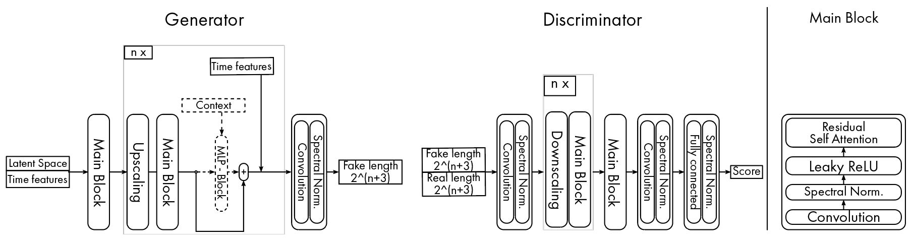
Figure 1: Left: Architecture of our proposed model, PSA-GAN. The generator contains $n$ blocks where each doubles the size of the output, by linear interpolation. It contains (dashed drawing) a multi layer perceptron block, that incorporates knowledge of the past in the generator. This block is used in the PSA-GAN-C model. The discriminator contains $n$ blocks that halve the size of the input using average pooling. Right: The main block used in the generator and discriminator.

Spectral Normalised Residual Self-Attention with Convolution

The generator and discriminator use a main function $m$ that is a composition of convolution, self-attention and spectral normalisation

$$m\circ f: \hskip 2.0pt\mathbb{R}^{n_{f}\times l}\rightarrow\mathbb{R}^{n_{f}\times l}$$ (1)

$$\hskip 2.0ptx\mapsto\gamma\operatorname{SA}(f(x))+f(x)$$

where $f(x)=\operatorname{LR}(\operatorname{SN}(c(x)))$ and $m(y)=\gamma\operatorname{SA}(y)+y$, $c$ is a one dimensional convolution operator, $\operatorname{LR}$ the LeakyReLU operator (Xu et al., 2015), $\operatorname{SN}$ the spectral normalisation operator (Miyato et al., 2018) and $\operatorname{SA}$ the self-attention module. The variable $n_{f}$ is the number of in and out-channels of $c$, $l$ is the length of the sequence. Following the work of (Zhang et al., 2019a), the parameter $\gamma$ is learnable. It is initialized to zero to allow the network to learn local features directly from the building block $f$ and is later enriched with distant features as the absolute value of gamma increases, hereby more heavily factoring the self-attention term $\operatorname{SA}$. The module $m$ is referenced as residual self-attention in Figure 1 (right).

Downscaling and Upscaling

The following sections mention upscaling ($\operatorname{UP}$) and downscaling ($\operatorname{DOWN}$) operators that double and halve the length of the time series, respectively. In this work, the upscaling operator is a linear interpolation and the downscaling operator is the average pooling.

PSA-GAN PSA-GAN is a progressively growing GAN (Karras et al., 2017); thus, trainable modules are added during training. Hereby, we model the generator and discriminator as a composition of functions: $G=g_{L+1}\circ...\circ g_{1}$ and $D=d_{1}\circ...\circ d_{L+1}$ where each function $g_{i}$ and $d_{i}$ for $i\in[1,L+1]$ corresponds to a module of the generator and discriminator.

Generator

As a preprocessing step, we first map the concatenated input $[\mathbf{n},\phi(i),\mathbf{X}_{t:t+\tau-1}]$ from a sequence of length $\tau$ to a sequence of length 8, denoted by $\tilde{Z}_{0}$, using average pooling. Then, the first layer of the generator $g_{1}$ applies the main function $m$:

$$g_{1}:\hskip 2.0pt\mathbb{R}^{n_{f}\times 2^{3}} \rightarrow\mathbb{R}^{n_{f}\times 2^{3}}$$ (2)

$$\hskip 2.0pt\tilde{Z}_{0} \mapsto\tilde{Z}_{1}=m\circ f(\tilde{Z}_{0})$$

For $i\in[2,L]$, $g_{i}$ maps an input sequence $\tilde{Z}_{i-1}$ to an output sequence $\tilde{Z}_{i}$ by applying an upscaling of the input sequence and the function $m\circ f$:

$$g_{i}:\hskip 2.0pt\mathbb{R}^{n_{f}\times 2^{i+1}} \rightarrow\mathbb{R}^{n_{f}\times 2^{i+2}}$$ (3)

$$\hskip 2.0pt\tilde{Z}_{i-1} \mapsto\tilde{Z}_{i}=m\circ f(\operatorname{UP}(\tilde{Z}_{i-1}))$$

The output of $g_{i}$ is concatenated back to the time features $\mathbf{X}_{t:t+\tau-1}$ and forwarded to the next block.

Lastly, the final layer of the generator $g_{L+1}$ reshapes the multivariate sequence $\tilde{Z}_{L}$ to a univariate time series $\hat{Z}_{i,t,\tau}$ of length $\tau=2^{L+3}$ using a one dimensional convolution and spectral normalisation.

Discriminator

The architecture of the discriminator mirrors the architecture of the generator. It maps the generator’s output $\hat{Z}_{i,t,\tau}$ and the time features $\mathbf{X}_{t:t+\tau-1}$ to a score $d$. The first module of the discriminator $d_{L+1}$ uses a one dimensional convolution $c_{1}$ and a LeakyReLU activation function:

$$d^{{}^{\prime}}_{L+1}:\hskip 2.0pt\mathbb{R}^{1+D,\tau} \rightarrow\mathbb{R}^{n_{f},\tau}$$ (4)

$$\hskip 2.0pt(\tilde{Z}_{L+1},\mathbf{X}_{t:t+\tau-1})\mapsto\tilde{Y}_{L} =\operatorname{SN}(\operatorname{LR}(c_{1}(\tilde{Z}_{L+1},\mathbf{X}_{t:t+\tau-1}))$$

For $i\in[L+1,2]$, the module $d_{i}$ applies a downscale operator and the main function $m$:

$$d_{i}:\hskip 2.0pt\mathbb{R}^{n_{f}\times 2^{i+2}} \rightarrow\mathbb{R}^{n_{f}\times 2^{i+1}}$$ (5)

$$\hskip 2.0ptY_{i} \mapsto Y_{i-1}=\operatorname{DOWN}(m(Y_{i}))$$

The last module $d_{1}$ turns its input sequence into a score:

$$d_{1}:\hskip 2.0pt\mathbb{R}^{n_{f}\times 2^{3}} \rightarrow\mathbb{R}$$ (6)

$$\hskip 2.0ptY_{1}\mapsto Y_{0} =\operatorname{SN}(\operatorname{FC}(\operatorname{LR}(\operatorname{SN}(c(m(Y_{1}))))))$$

where $\operatorname{FC}$ is a fully connected layer.

PSA-GAN-C We introduce another instantiation of PSA-GAN in which we forward to each generator block $g_{i}$ knowledge about the past. The knowledge here is a sub-series $\hat{Z}_{i,t-L_{C},L_{C}}$ in the range $[t-L_{C},t-1]$, with $L_{C}$ being the context length. The context $\hat{Z}_{i,t-L_{C},L_{C}}$ is concatenated along the feature dimension, i.e. at each time step, to the output sequence of $g_{i}$. It is then passed through a two layers perceptron to reshape the feature dimension and then added back to the output of $g_{i}$.

3.1 Loss functions

PSA-GAN is trained via the LSGAN loss (Mao et al., 2017), since it has been shown to address mode collapse (Mao et al., 2017). Furthermore, least-squares type losses in embedding space have been shown to be effective in the time series domain (Mogren, 2016; Yoon et al., 2019). Additionally, we use an auxiliary moment loss to match the first and second order moments between the batch of synthetic samples and a batch of real samples:

$$\operatorname{ML}\left(\hat{\mathbf{Z}}_{\tau},\mathbf{Z}_{\tau}\right)=\left|\mu\left(\hat{\mathbf{Z}}_{\tau}\right)-\mu\left(\mathbf{Z}_{\tau}\right)\right|+\left|\sigma\left(\hat{\mathbf{Z}}_{\tau}\right)-\sigma\left(\mathbf{Z}_{\tau}\right)\right|$$ (7)

where $\mu$ is the mean operator and $\sigma$ is the standard deviation operator. The real and synthetic batches have their time index and time series index aligned. We found this combination to work well for PSA-GAN empirically. Note that the choice of loss function was not the main focus of this study and we think that our choice can be improved in future research.

Training procedures

GANs are notoriously difficult to train, have hard-to-interpret learning curves, and are susceptible to mode collapse. The training procedure to address those issues together with other training and tuning details is presented in Appendix B–E.

4 Experiments

The evaluation of synthetic time series data from GAN models is challenging and there is no widely accepted evaluation scheme in the time series community. We evaluate the GAN models by two guiding principles: i) Measuring to what degree the time series recover the statistics of the training dataset. ii) Measuring the performances of the GAN models in challenging, downstream forecasting scenarios.

For i), we introduce the Context-FID (Context-Frechet Inception distance) score to measure whether the GAN models are able to recover the training set statistics. The FID score is widely used for evaluating synthetic data in computer vision (Heusel et al., 2017) and uses features from an inception network (Szegedy et al., 2016) to compute the difference between the real and synthetic sample statistics in this feature space. In our case, we are interested in how well the the synthetic time series windows ”fit” into the local context of the time series. Therefore, we use the time series embeddings from Franceschi et al. (2019) to learn embeddings of time series that fit into the local context. Note that we train the embedding network for each dataset separately. This allows us to directly quantify the quality of the synthetic time series samples (see Appendix D for details).

For ii), we set out to mimic several challenging time series forecasting tasks that are common for time series forecasting practitioners. These tasks often have in common that practitioners face missing or corrupted data during training or inference. Here, we set out to use the synthetic samples to complement an established baseline model, DeepAR, in these forecasting tasks. These tasks are: far-forecasting and missing values during inference, missing values during training, cold starts, and data augmentation. We evaluate these tasks by the normalized root mean squared distance (NRMSE). Additionally, we evaluate PSA-GAN model when used as a forecasting model. Note that, where applicable, we re-train our GAN models on the modified datasets to ensure that they have the same data available as the baseline model during the downstream tasks.

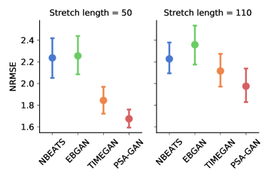
Figure S3: Performance of using different GAN models for imputation in the missing value stretch length experiment using NBEATS as the forecasting model. Markers denote the mean NRMSE averaged over datasets and error bars the 68% confidence interval over ten runs.

We also considered NBEATS (Oreshkin et al., 2020a) and Temporal Fusion Transformer (TFT) (Lim et al., 2021) as alternative forecasting models. However, we found that DeepAR performed best in our experiments and therefore we report these results in the main text (see Appendix F for experiment details). Please refer to Appendix G for the evaluation of NBEATS and TFT (Tables S2–S6 and Figures S3–S6).

In addition, we perform an ablation study of our model and discuss whether the Context-FID scores are indicative for downstream forecasting tasks.

4.1 Datasets and Baselines

We use the following public, standard benchmark datasets in the time series domain: M4, hourly time series competition data (414 time series)  (Makridakis et al., 2020); Solar, hourly solar energy collection data in Alabama State (137 stations) (Lai et al., 2018); Electricity, hourly electricity consumption data (370 customers) (Dheeru & Karra Taniskidou, 2017); Traffic: hourly occupancy rate of lanes in San Francisco (963 lanes) (Dheeru & Karra Taniskidou, 2017). Unless stated otherwise, we split all data into a training/test set with a fixed date and use all data before that date for training. For testing, we use a rolling window evaluation with a window size of 32 and seven windows. We minmax scale each dataset to be within $[0,1]$ for all experiments in this paper (we scale the data back before evaluating the forecasting experiments). In lieu of finding public datasets that represent the downstream forecasting tasks, we modify each the datasets above to mimic each tasks for the respective experiment (see later sections for more details).

We compare PSA-GAN with different GAN models from the literature (TIMEGAN (Yoon et al., 2019) and EBGAN (Zhao et al., 2017)). In what follows PSA-GAN-C and PSA-GAN denote our proposed model with and without context, respectively. In the forecasting experiments, we use the GluonTS (Alexandrov et al., 2020) implementation of DeepAR which is a well-performing forecasting model and established baseline (Salinas et al., 2020).

4.2 Direct Evaluation with Context-FID Scores

Dataset	Length	EBGAN	TIMEGAN	PSA-GAN	PSA-GAN-C
Electricity	64	$2.07$$\pm 0.3$	$0.77$$\pm 0.12$	$0.018$$\pm 0.009$	$\mathbf{0.011}$$\pm 0.002$
	128	$1.93$$\pm 0.28$	$1.03$$\pm 0.13$	$0.03$$\pm 0.01$	$\mathbf{0.022}$$\pm 0.01$
	256	$3.02$$\pm 0.25$	$1.58$$\pm 0.08$	$0.042$$\pm 0.018$	$\mathbf{0.036}$$\pm 0.02$
M4	64	$0.93$$\pm 0.15$	$0.93$$\pm 0.1$	$\mathbf{0.113}$$\pm 0.051$	$0.158$$\pm 0.088$
	128	$2.53$$\pm 0.27$	$0.6$$\pm 0.07$	$\mathbf{0.156}$$\pm 0.072$	$0.22$$\pm 0.11$
	256	$2.08$$\pm 0.13$	$0.89$$\pm 0.13$	$0.356$$\pm 0.125$	$\mathbf{0.235}$$\pm 0.066$
Solar-Energy	64	$0.48$$\pm 0.11$	$0.13$$\pm 0.02$	$0.012$$\pm 0.003$	$\mathbf{0.004}$$\pm 0.001$
	128	$1.87$$\pm 0.43$	$0.22$$\pm 0.05$	$0.007$$\pm 0.001$	$\mathbf{0.002}$$\pm 0.001$
	256	$2.38$$\pm 0.43$	$0.09$$\pm 0.02$	$0.064$$\pm 0.002$	$\mathbf{0.004}$$\pm 0.001$
Traffic	64	$2.65$$\pm 0.15$	$0.59$$\pm 0.06$	$0.241$$\pm 0.041$	$\mathbf{0.058}$$\pm 0.009$
	128	$2.09$$\pm 0.26$	$2.13$$\pm 0.12$	$0.182$$\pm 0.029$	$\mathbf{0.044}$$\pm 0.005$
	256	$1.86$$\pm 0.14$	$1.82$$\pm 0.12$	$\mathbf{0.13}$$\pm 0.017$	$0.488$$\pm 0.027$

Table 1: Context FID-scores (lower is better) of PSA-GAN and baselines. We score 5120 randomly selected windows and report the mean and standard deviation.

Table 1 shows the Context-FID scores for PSA-GAN, PSA-GAN-C and baselines. For all sequence lengths, we find that PSA-GAN or PSA-GAN-C consistently produce the lowest Context-FID scores. For a sequence length of 256 time steps, TIMEGAN is the second best performing model for all datasets. Note that even though using a context in the PSA-GAN model results in the best overall performance, we are interested to use the GAN in downstream tasks where the context is not available. Thus, the next section will use PSA-GAN without context, unless otherwise stated.

4.3 Evaluation on Forecasting Tasks

In this section, we present the results of the forecasting tasks. We find that synthetic samples do not improve over baselines in all cases. However, we view these results as a first attempt to use GAN models in these forecasting tasks and believe that future research could improve over our results.

Far-forecasting:

In this experiment, we forecast far into the future by assuming that the data points between the training end time and the rolling evaluation window are not observed. For example, the last evaluation window would have $32*6$ unobserved values between the training end time and the forecast start date. This setup reflects two possible use cases: Forecasting far into the future (where no context data is available) and imputing missing data during inference because of a data outage just before forecasting. Neural network-based forecasting models such as DeepAR struggle under these conditions because they rely on the recent context and need to impute these values during inference. Furthermore, DeepAR only imputes values in the immediate context and not for the lagged values. Here, we use the GAN models during inference to fill the missing observations with synthetic data. As a baseline, we use DeepAR and impute the missing observations of lagged values with a moving average (window size 10) during inference. Here, we find that using the synthetic data from GAN models drastically improve over the DeepAR baseline and using samples from PSA-GAN results into the lowest NRMSE for three out of four datasets (see left Table in Figure 2). Figure 2 also shows the NRMSE as a function of the forecast window. Figure 3 shows an example of a imputed time series and the resulting forecast from the Electricity dataset when using PSA-GAN.

Figure 2: NRMSE of far-forecasting experiments (lower is better). Mean and confidence intervals are obtained by re-running each method ten times. Left: NRMSE average over different forecast windows. DeepAR is only run on the real time series data. The other models correspond to DeepAR and one of the GAN models for filling missing observations. Right: NRMSE by forecast window. The first window will have no missing values during inference (we forecast the first 32 steps after the training range) and we increase the missing values during inference with each window (the last window will have $32*6$ missing values). For DeepAR, the NRMSE increases noticeably at the fourth forecast window while using PSA-GAN to impute the missing values at inference keeps the NRMSE low.

	NRMSE
Dataset	Electricity	M4	Solar	Traffic
Model
DeepAR	$3.31$$\pm 0.78$	$0.84$$\pm 0.44$	$1.43$$\pm 0.02$	$1.0$$\pm 0.15$
EBGAN	$2.46$$\pm 0.3$	$1.26$$\pm 0.29$	$2.02$$\pm 0.07$	$0.9$$\pm 0.22$
TIMEGAN	$1.57$$\pm 0.25$	$1.32$$\pm 0.13$	$\mathbf{1.21}$$\pm 0.05$	$0.86$$\pm 0.17$
PSA-GAN	$\mathbf{0.99}$$\pm 0.44$	$\mathbf{0.62}$$\pm 0.3$	$1.22$$\pm 0.05$	$\mathbf{0.59}$$\pm 0.2$

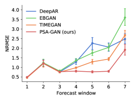
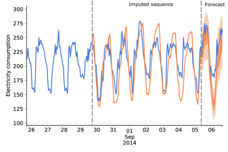
Figure 3: Example of the far-forecasting experiment for the Electricity dataset. True data is shown in blue and the imputed sequence and forecasts of the model in orange. The orange line between the dashed lines corresponds to the PSA-GAN imputed sequence and is used by DeepAR for forecasting. Note that this part is unobserved in this experiment. The imputed sequence allows to generate a reasonable forecast, even if many data points before the forecast start date are unobserved.

Missing Value Stretches:

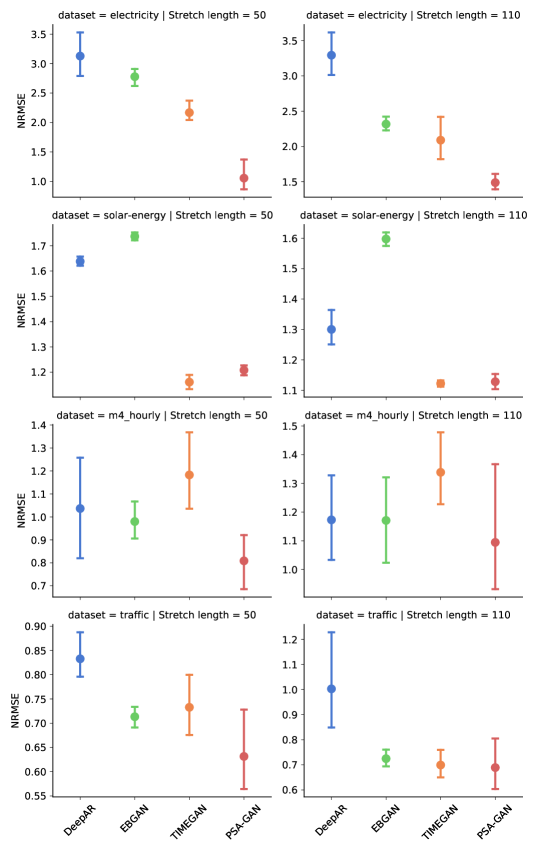
Figure S1: Detailed performance of using different GAN models for imputation in the missing value stretch length experiment. Markers denote the mean NRMSE averaged over ten runs and error bars represent the 95% confidence interval. For 50 and 110 missing value stretch length, using PSA-GAN to impute missing values results in the lowest error for three out of four datasets.

Missing values are present in many real world time series applications and are often caused by outages of a sensor or service (Zhang et al., 2019b). Therefore, missing values in real-world scenarios are often not evenly distributed over the time series but instead form missing value ”stretches”. In this experiment, we simulate missing value stretches and remove time series values of length 50 and 110 from the datasets. This results into 5.4-7.7% missing values for a stretch length of 50 and and 9.9-16.9% missing values for a stretch length of 110 (depending on the dataset.) Here, we split the training dataset into two parts along the time axis and only introduce missing values in the second part. We use the first (unchanged) part of the training dataset to train the GAN models and both parts of the training set to train DeepAR. We then use the GAN models to impute missing values during training and inference of DeepAR. Figure 4 shows that using the GAN models to impute missing values during training DeepAR on data with missing value stretches reduces its forecasting error. While all GAN models reduce the NRMSE in this setup, PSA-GAN is most effective in reducing the error in this experiment. See Figure S1 for a detailed split by dataset.

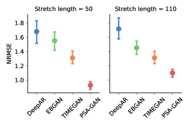
Figure 4: Performance of using different GAN models for imputation in the missing value stretch length experiment. Markers denote the mean NRMSE averaged over datasets and error bars the 68% confidence interval over ten runs. For 50 and 110 missing value stretch length, using PSA-GAN to impute missing values results in the lowest overall error, whereas DeepAR returns the highest.

Cold Starts:

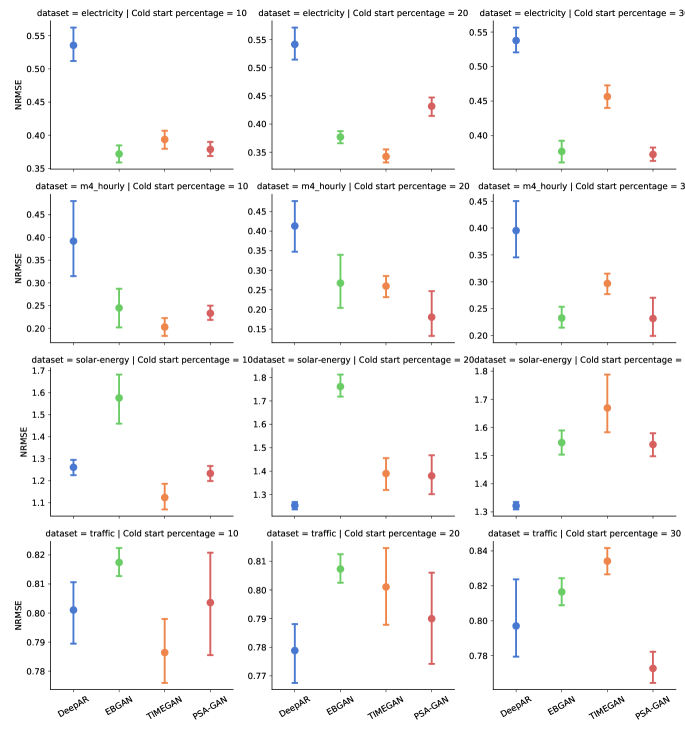
Figure S2: Detailed performance of using different GAN models for the cold start experiment. Markers denote the mean NRMSE averaged over ten runs and error bars the 95% confidence interval. TIMEGAN and PSA-GAN improve over DeepAR in three out of four datasets.

In this experiment, we explore whether the GAN models can support DeepAR in a cold start forecasting setting. Cold starts refer to new time series (like a new product in demand forecasting) for which little or no data is available. Here, we randomly truncate 10%, 20%, and 30% of the time series from our datasets such that only the last 24 (representing 24 hours of data) values before inference are present. We only consider a single forecasting window in this experiment. We then again use the GAN models to impute values for the lags and context that DeepAR conditions for forecasting the cold start time series. Figure 5 shows the forecasting error of the different models for the cold start time series only. In this experiment, PSA-GAN and TIMEGAN improve the NRMSE over DeepAR and are on-par overall (mean NMRSE $0.70$ and $0.71$ for PSA-GAN and TIMEGAN, respectively). See Figure S2 for a detailed split by dataset.

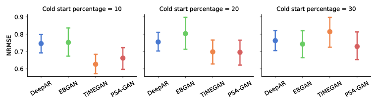
Figure 5: Performance of using different GAN models for imputation in the cold start experiment. Markers denote the mean NRMSE averaged over datasets and error bars the 68% confidence interval over ten runs. Note that this figure only shows the error of the cold start time series. Overall, TIMEGAN and PSA-GAN improve the NRMSE over DeepAR in this setup, while PSA-GAN is the best method when 30% of time series are cold starts.

Data Augmentation:

In this experiment, we average the real data and GAN samples to augment the data during training.  During inference, DeepAR is conditioned on real data only to generate forecasts. In Table 2 we we can see that none of the GAN models for data augmentation consistently improves over DeepAR. Overall, TIMEGAN is the best-performing GAN model but plain DeepAR still performs better. This finding is aligned with recent work in the image domain where data augmentation with GAN samples does not improve a downstream task (Ravuri & Vinyals, 2019). We hypothesize that the GAN models cannot improve in the data augmentation setup because they are trained to generate realistic samples and not necessarily to produce relevant invariances. Furthermore, the dataset sizes might be sufficient for DeepAR to train a well-performing model and therefore the augmentation might not be able to reduce the error further. More research is required to understand whether synthetic data can improve forecasting models via data augmentation.

	NRMSE
Dataset	Electricity	M4	Solar	Traffic
Model
DeepAR	$\mathbf{0.49}$$\pm 0.03$	$\mathbf{0.26}$$\pm 0.02$	$1.07$$\pm 0.01$	$\mathbf{0.45}$$\pm 0.01$
EBGAN	$0.64$$\pm 0.05$	$0.32$$\pm 0.09$	$1.18$$\pm 0.03$	$0.50$$\pm 0.03$
TIMEGAN	$0.56$$\pm 0.05$	$0.28$$\pm 0.02$	$\mathbf{1.06}$$\pm 0.02$	$0.47$$\pm 0.004$
PSA-GAN	$0.64$$\pm 0.22$	$0.3$$\pm 0.04$	$1.07$$\pm 0.03$	$0.50$$\pm 0.11$

Table 2: NRMSE accuracy comparison of data augmentation experiments (lower is better, best method in bold). Mean and 95% confidence intervals are obtained by re-running each method five times. DeepAR is only run on the real time series data. The other models correspond to DeepAR and one of the GAN models for data augmentation.

Forecasting Experiments:

In this experiment, we use the GAN models directly for forecasting (Table 3, example samples in Appendix H). We can see that DeepAR consistently performs best. This is expected as DeepAR takes into account context information and lagged values. This kind of information is not available to the GAN models. To test this we further consider PSA-GAN-C, i.e. PSA-GAN with 64 previous time series values as context, and further evaluate DeepAR with drawing lags only from the last 64 values (DeepAR-C). We can see that in this case PSA-GAN-C outperforms DeepAR-C in 3 out of 4 datasets and PSA-GAN performs on par with DeepAR-C. Moreover, both PSA-GAN and PSA-GAN-C are the best performing GAN models. Adding lagged values to the GAN models as context could further improve their performance and adversarial/attention architectures have been previously used for forecasting (Wu et al., 2020).

	NRMSE
Dataset	Electricity	M4	Solar	Traffic
Model
DeepAR	$\mathbf{0.49}$$\pm 0.03$	$\mathbf{0.26}$$\pm 0.02$	$\mathbf{1.07}$$\pm 0.01$	$\mathbf{0.45}$$\pm 0.01$
DeepAR-C	$1.43$$\pm 0.40$	$0.73$$\pm 0.46$	$0.95$$\pm 0.01$	$0.89$$\pm 0.16$
EBGAN	$3.63$$\pm 0.07$	$1.14$$\pm 0.01$	$2.31$$\pm 0.01$	$2.02$$\pm 0.00$
TIMEGAN	$3.04$$\pm 0.00$	$1.12$$\pm 0.00$	$1.83$$\pm 0.00$	$1.13$$\pm 0.00$
PSA-GAN	$1.53$$\pm 0.00$	$0.61$$\pm 0.00$	$1.35$$\pm 0.00$	$0.66$$\pm 0.00$
PSA-GAN-C	$1.18$$\pm 0.00$	$0.33$$\pm 0.00$	$1.32$$\pm 0.00$	$0.57$$\pm 0.00$

Table 3: NRMSE accuracy comparison of forecasting experiments (lower is better, best method in bold). Mean and 95% confidence intervals are obtained by re-running each method five times. DeepAR-C and PSA-GAN-C use the same 64 previous values as context. Among GAN models PSA-GAN and PSA-GAN-C perform best.

4.4 Ablation Study

Figure 6 shows the results of our ablation study where we disable important components of our model: moment loss, self-attention, and fading in of new layers. We measure the performance of the ablation models by Context-FID score. Overall, our propost logog ed PSA-GAN model performs better than the ablations which confirms that these components contribute to the performance of the model.

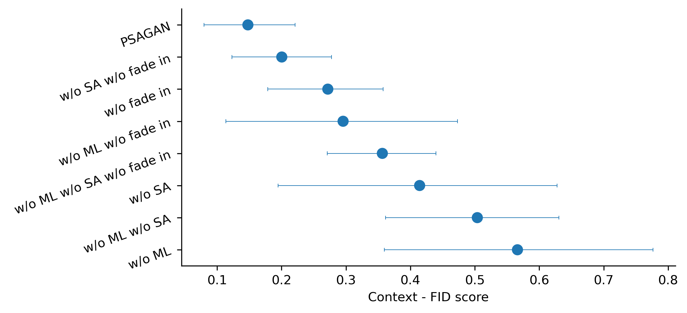
Figure 6: We perform an ablation study by disabling moment loss, self-attention, and fading in of new layers of PSA-GAN. We show the mean performance over three runs on four datasets and the 68% confidence interval. PSA-GAN has the lowest Context-FID score which confirms that the proposed model requires these components for good performance. SA: Self-attention, ML: Moment loss, fade in: Progressive fade in of new layers

4.5 Low Context-FID Score Models Correspond to Best-performing Forecasting Models

One other observation is that the lowest Context-FID score models correspond to the best models in the data augmentation and far-forecasting experiments. PSA-GAN and TIMEGAN produce the lowest Context-FID samples and both models also improve over the baseline in most downstream tasks. Overall, PSA-GAN has lowest Context-FID and also outperforms the other models in the downstream forecasting tasks, except for the cold start task. Additionally, we calculated the Context-FID scores for the ablation models mentioned in Figure 6 (but with a target length of $32$) and the NRMSE of these models in the forecasting experiment (as in Table 3). We find that the Pearson correlation coefficient between the Context-FID and forecasting NRMSE is 0.71 and the Spearman’s rank correlation coefficient is 0.67, averaged over all datasets. All datasets (except Traffic) have a correlation coefficient of at least 0.73 in either measure (see Table S1 in the Appendix).

5 Conclusion

We have presented PSA-GAN, a progressive growing time series GAN augmented with self-attention, that produces long realistic time series and improves downstream forecasting tasks that are challenging for deep learning-based time series models. Furthermore, we introduced the Context-FID score to assess the quality of synthetic time series samples produced by GAN models. We found that the lowest Context-FID scoring models correspond to the best-performing models in downstream tasks. We believe that time series GANs that scale to long sequences combined with a reliable metric to assess their performance might lead to their routine use in time series modeling.

6 Reproducibility statement

Details necessary for reproducing our experiments are given in the Appendix. In particular, details on training are provided in Sections B and C, together with hyperparameter tuning in Section E and further experimental settings in Section F. The code we used in the paper is available under:
https://github.com/mbohlkeschneider/psa-gan and we will additionally disseminate PSA-GAN via GluonTS: https://github.com/awslabs/gluon-ts.

Appendix

Appendix A Time Series Features

We use time-varying features to represent the time dimension for the GAN models to enable training on time series windows sampled from the full-length time series . We use HourOfDay, DayOfWeek, DayOfMonth and DayOfYear features. Each feature is encoded using a single index number (for example, between $[0,365[$ for DayOfYear) and normalized to be within [-0.5, 0.5]. We also use an age feature to represent the age of the time series to be $log(2.0+t)$ where $t$ is the time index. Additionally, we embed the index of the individual time series into a 10 dimensional vector with an embedding network to and use it as a non time-varying feature. DeepAR uses the same features in forecasting.

Appendix B Training Procedure

PSA-GAN uses spectral normalization and progressive fade-in of new layers to stabilize training.

Progressive fade in of new layers

As training progresses, new layers are added to double the length of time series. However, simply adding new untrained layers drastically changes the number of parameters and the loss landscape, which destabilizes training. Progressive fade in of new layers is a technique introduce by Karras et al., 2017 to mitigate this effect where each layer $g_{i}$ and $d_{i}$ is smoothly introduced. For $i\in[2,L]$ the fade in of new layers is written as:

$$g_{i}: \mathbb{R}^{n_{f}\times 2^{i+1}}\rightarrow\mathbb{R}^{n_{f}\times 2^{i+2}}$$ (8)

$$\tilde{Z}_{i-1}\mapsto\tilde{Z}_{i}=\alpha m(\operatorname{UP}(\tilde{Z}_{i-1}))+(1-\alpha)\operatorname{UP}(\tilde{Z}_{i-1})$$

$$d_{i}: \mathbb{R}^{n_{f}\times 2^{i+2}}\rightarrow\mathbb{R}^{n_{f}\times 2^{i+1}}$$ (9)

$$Y_{i}\mapsto Y_{i-1}=\alpha\operatorname{DOWN}(m(Y_{i}))+(1-\alpha)\operatorname{DOWN}(Y_{i})$$

where $\alpha$ is a scalar initialized to be zero and grows linearly to one over 500 epochs.

Spectral Normalisation

Both the generator and the discriminator benefit from using spectral normalisation layers. In the discriminator, Spectral Normalisation stabilizes training (Miyato et al., 2018). It constrains the Lipschitz constant of the discriminator to be bounded by one. In the generator the spectral normalisation stabilises the training and avoids escalation of the gradient magnitude (Zhang et al., 2019a).

Appendix C Training Details

All GAN models in this paper have been implemented using PyTorch from Paszke et al. (2019).

PSA-GAN has been trained over 6500 epochs, where a new block is added every 1000 epochs and is faded over 500 epochs. At each epoch, PSA-GAN trains on 100 batches of size 512. It optimises its parameters using the Adam (Kingma & Ba, 2014) with a learning rate of $0.0005$ and betas of $(0.9,0.999)$ for both the generator and the discriminator.

PSA-GAN (and its variants) has been trained on ml.p2.xlarge Amazon instances for $21$ hours.

The number of in-channels and out-channels $n_{f}$ in the Main Block (Figure 1, Right) equals $32$. The number of out-channels in the convolution layer $c$ equals $1$ (Eq.6 ). The number of time features $D$ equals $15$.

For the case of PSA-GAN-C, the MLP block is a two layers perceptron with LeakyReLU. It incorporates knowledge of the past by selecting the $L_{C}=64$ time points and concatenates them with its input.

Appendix D Context-FID Score on Time Series Embeddings

To compute the Context-FID, we replace InceptionV3 (Szegedy et al., 2016) with the encoder $E$ of Franceschi et al. (2019), which we train separately for each dataset.
Our proposed Context-FID score is computed as follows: we first select a time range $[t,t+\tau]$. We then sample a batch of synthetic time series $\mathbf{\hat{Z}}_{t,\tau}=[\hat{Z}_{1,t,\tau},...,\hat{Z}_{N,t,\tau}]$ and a batch of real time series $\mathbf{Z}_{t,\tau}=[Z_{1,t,\tau},...,Z_{N,t,\tau}]$ that we encode with $E$ into $\mathbf{\hat{Z}}^{e}_{t,\tau}$ and $\mathbf{Z^{e}}_{t,\tau}$ respectively. Finally, we compute the FID score of the embeddings.

Appendix E Hyperparameter tuning

We did limited hyperparameter tuning in this study to find default hyperparemters that perform well across datasets. We performed the following grid-search: the batch size, the number of batches used per epoch, the presence of Self-attention and the presence of the Progressive fade in of new layers mechanism explained in section B, paragraph B.
The range considered for each hyper-parameter is: batch size : $[64,128,256,512]$, the number of batches used per epoch: $[50,100,200]$, the presence of Self-attention: $[\text{True},\text{False}]$ and the presence of the Progressive fade in of new layers: $[\text{True},\text{False}]$.

The set of hyperparameters is shared across the four datasets we train PSA-GAN on (which means we do not tune hyperparameters per datasets). We select the final hyperparameter set by lowest Context-FID score on the training set, averaged across all datasets.

Appendix F Forecasting Experiment Details

We use the DeepAR (Salinas et al., 2020) implementation in GluonTS (Alexandrov et al., 2020) for the forecasting experiments. We use the default hyperparameters of DeepAR with the following exceptions: epochs=100, num batches per epoch=100, dropout rate=0.01, scaling=False, prediction length=32, context length=64, use feat static cat=True. We use the Adam optimizer with a learning rate of $1\mathrm{e}{-3}$ and weight decay of $1\mathrm{e}{-8}$ . Additionally, we clip the gradient to $10.0$ and reduce the learning rate by a factor of $2$ for every $10$ consecutive updates without improvement, up to a minimum learning rate of $5\mathrm{e}{-5}$. DeepAR also uses lagged values from previous time steps that are used as input to the LSTM at each time step $t$. We set the time series window size that DeepAR samples to 256 and truncate the default hourly lags to fit the context window, the prediction window, and the longest lag into the window size 256. We use the following lags: [1, 2, 3, 4, 5, 6, 7, 23, 24, 25, 47, 48, 49, 71, 72, 73, 95, 96, 97, 119, 120, 121, 143, 144, 145].

For NBEATS (Oreshkin et al., 2020a), we use the default parameters and set the trainer settings to epochs=100, num batches per epoch=50. Note that in the original paper, NBEATS is an ensemble of 180 networks. Due to the high computational cost, we only ensemble three networks with the settings context length=64, context length=96, context length=128 and mean absolute percentage error as the loss function.

For TFT (Lim et al., 2021), we use the default hyperparameters except: epochs=100, num batches per epoch=50, context length=128.

For all methods, we used the implementations available in GluonTS (Alexandrov et al., 2020).

Appendix G Additional Experiments

	Pearson	Spearman
Traffic	0.597	0.609
M4	0.858	0.455
Solar	0.852	0.773
Electricity	0.533	0.891

Table S1: Pearson and Spearman rank-order correlation coefficient between the Context-FID score and NRMSE for different datasets. These results suggest that low Context-FID scores indicate low error in forecasting and therefore Context-FID could be a useful score to develop GAN models in the time series domain.

Table S2: NRMSE of far-forecasting experiments with NBEATS as the forecasting model (lower is better). Mean and confidence intervals are obtained by re-running each method ten times.

	NRMSE
Dataset	Electricity	M4	Solar	Traffic
Model
NBEATS	$5.29\pm 0.28$	$1.92\pm 0.04$	$2.08\pm 0.0$	$0.94\pm 0.02$
EBGAN	$3.59\pm 0.21$	$1.76\pm 0.03$	$2.07\pm 0.0$	$0.96\pm 0.0$
TIMEGAN	$2.06\pm 0.02$	$1.75\pm 0.01$	$2.07\pm 0.0$	$0.8\pm 0.01$
PSA-GAN	$\mathbf{1.30}\pm 0.04$	$\mathbf{0.4}\pm 0.01$	$2.07\pm 0.0$	$\mathbf{0.65}\pm 0.0$

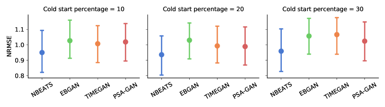
Figure S4: Performance of using different GAN models for imputation in the cold start experiment using NBEATS as the forecasting model. Markers denote the mean NRMSE averaged over datasets and error bars the 68% confidence interval over ten runs. Note that this figure only shows the error of the cold start time series.

Table S3: NRMSE accuracy comparison of data augmentation experiments (lower is better) using NBEATS as the forecasting model. Mean and 95% confidence intervals are obtained by re-running each method five times.

	NRMSE
Dataset	Electricty	M4	Solar	Traffic
Model
NBEATS	$0.86\pm 0.06$	$\mathbf{0.28}\pm 0.01$	$2.07\pm 0.0$	$0.58\pm 0.0$
EBGAN	$0.74\pm 0.03$	$0.31\pm 0.01$	$2.08\pm 0.0$	$0.58\pm 0.01$
TIMEGAN	$\mathbf{0.58}\pm 0.01$	$0.28\pm 0.01$	$2.08\pm 0.0$	$\mathbf{0.51}\pm 0.0$
PSA-GAN	$0.92\pm 0.06$	$0.3\pm 0.01$	$\mathbf{1.97}\pm 0.02$	$0.54\pm 0.01$

Table S4: NRMSE of far-forecasting experiments with Temporal Fusion Transformer (TFT) as the forecasting model (lower is better). Mean and confidence intervals are obtained by re-running each method ten times.

	NRMSE
Dataset	Electricity	M4	Solar	Traffic
Model
TFT	$4.51\pm 0.02$	$1.78\pm 0.04$	$1.74\pm 0.02$	$0.94\pm 0.0$
EBGAN	$3.54\pm 0.22$	$1.5\pm 0.05$	$2.5\pm 0.13$	$0.76\pm 0.02$
TIMEGAN	$2.03\pm 0.05$	$1.71\pm 0.04$	$\mathbf{1.26}\pm 0.03$	$0.82\pm 0.03$
PSA-GAN	$\mathbf{1.97}\pm 0.05$	$\mathbf{0.34}\pm 0.01$	$2.15\pm 0.13$	$\mathbf{0.70}\pm 0.0$

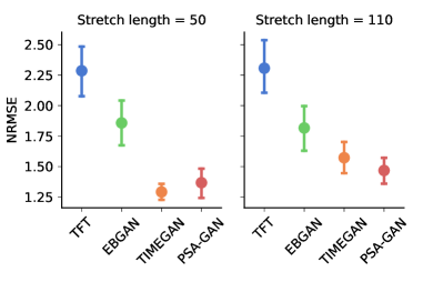
Figure S5: Performance of using different GAN models for imputation in the missing value stretch length experiment using Temporal Fusion Transformer (TFT) as the forecasting model. Markers denote the mean NRMSE averaged over datasets and error bars the 68% confidence interval over ten runs.

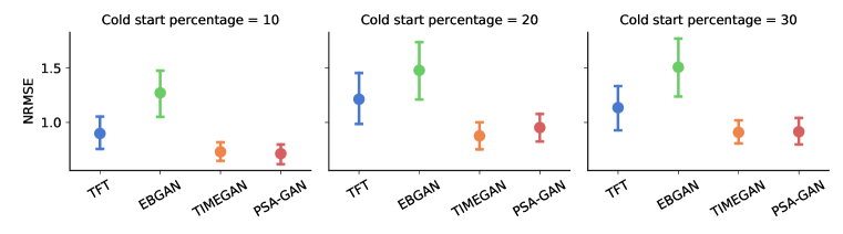
Figure S6: Performance of using different GAN models for imputation in the cold start experiment using Temporal Fusion Transformer (TFT) as the forecasting model. Markers denote the mean NRMSE averaged over datasets and error bars the 68% confidence interval over ten runs. Note that this figure only shows the error of the cold start time series.

Table S5: NRMSE accuracy comparison of data augmentation experiments (lower is better) using Temporal Fusion Transformer (TFT) as the forecasting model. Mean and 95% confidence intervals are obtained by re-running each method five times.

	NRMSE
Dataset	Electricity	M4	Solar	Traffic
Model
TFT	$\textbf{0.63}\pm 0.04$	$\textbf{0.26}\pm 0.02$	$1.29\pm 0.04$	$\textbf{0.40}\pm 0.0$
EBGAN	$0.9\pm 0.05$	$0.31\pm 0.01$	$\textbf{1.21}\pm 0.05$	$0.64\pm 0.01$
TIMEGAN	$0.83\pm 0.04$	$0.85\pm 0.06$	$1.28\pm 0.03$	$0.51\pm 0.01$
PSA-GAN	$0.94\pm 0.03$	$0.35\pm 0.02$	$1.64\pm 0.04$	$0.42\pm 0.0$

	NRMSE
Dataset	Electricity	M4	Solar	Traffic
Model
DeepAR	$\mathbf{0.49}$$\pm 0.03$	$\mathbf{0.26}$$\pm 0.02$	$\mathbf{1.07}$$\pm 0.01$	$0.45$$\pm 0.01$
NBEATS	$0.86$$\pm 0.06$	$0.28$$\pm 0.01$	$2.07$$\pm 0.00$	$0.58$$\pm 0.00$
TFT	$0.63$$\pm 0.04$	$0.26$$\pm 0.02$	$1.29$$\pm 0.04$	$\mathbf{0.40}$$\pm 0.00$
DeepAR-C	$1.43$$\pm 0.40$	$0.73$$\pm 0.46$	$0.95$$\pm 0.01$	$0.89$$\pm 0.16$
EBGAN	$3.63$$\pm 0.07$	$1.14$$\pm 0.01$	$2.31$$\pm 0.01$	$2.02$$\pm 0.00$
TIMEGAN	$3.04$$\pm 0.00$	$1.12$$\pm 0.00$	$1.83$$\pm 0.00$	$1.13$$\pm 0.00$
PSA-GAN	$1.53$$\pm 0.00$	$0.61$$\pm 0.00$	$1.35$$\pm 0.00$	$0.66$$\pm 0.00$
PSA-GAN-C	$1.18$$\pm 0.00$	$0.33$$\pm 0.00$	$1.32$$\pm 0.00$	$0.57$$\pm 0.00$

Table S6: Extended NRMSE accuracy comparison of forecasting experiments with NBEATS and Temporal Fusion Transformer (TFT) as additional forecasting models (lower is better).

Appendix H Sample forecasts

We present more sample forecasts under the framework of the forecasting experiment. In Figures S10–S10 we present sample forecast for Electricity, M4, Solar Energy, and Traffic datasets, respectively. We can see that the synthetic time series generated by PSA-GAN and PSA-GAN-C consistently convey a better approximation to the ground truth values. One can further observe that this task is particularly challenging for GANs as data generation is located in a time-frame that is not covered while training.

Figure S7: Sample forecasts for dataset Electricity

(a) EBGAN

(b) TIMEGAN

(c) PSA-GAN

(d) PSA-GAN-C

Figure S8: Sample forecasts for dataset M4

(a) EBGAN

(b) TIMEGAN

(c) PSA-GAN

(d) PSA-GAN-C

Figure S9: Sample forecasts for dataset Solar

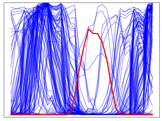
(a) EBGAN

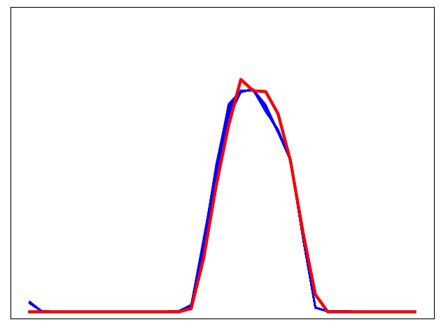
(b) TIMEGAN

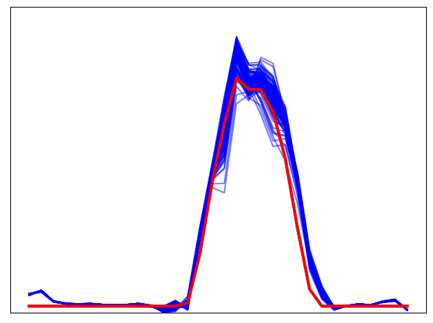
(c) PSA-GAN

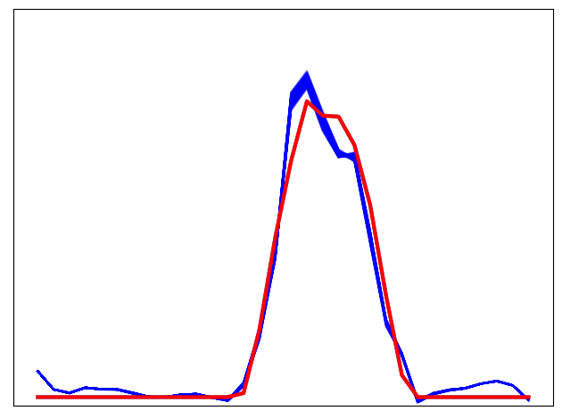
(d) PSA-GAN-C

Figure S10: Sample forecasts for dataset Traffic

(a) EBGAN

(b) TIMEGAN

(c) PSA-GAN

(d) PSA-GAN-C

References

- Alexandrov et al. (2020) Alexander Alexandrov, Konstantinos Benidis, Michael Bohlke-Schneider, Valentin Flunkert, Jan Gasthaus, Tim Januschowski, Danielle C. Maddix, Syama Rangapuram, David Salinas, Jasper Schulz, Lorenzo Stella, Ali Caner Türkmen, and Yuyang Wang. GluonTS: Probabilistic and neural time series modeling in python. Journal of Machine Learning Research, 21(116):1–6, 2020.
- Bai et al. (2018) Shaojie Bai, J. Zico Kolter, and Vladlen Koltun. An Empirical Evaluation of Generic Convolutional and Recurrent Networks for Sequence Modeling. arXiv:1803.01271, 2018.
- Brock et al. (2018) Andrew Brock, Jeff Donahue, and Karen Simonyan. Large Scale GAN Training for High Fidelity Natural Image Synthesis. arXiv:1809.11096, 2018.
- Cont (2001) R. Cont. Empirical properties of asset returns: stylized facts and statistical issues. Quantitative Finance, 1(2):223–236, feb 2001.
- Cui et al. (2016) Zhicheng Cui, Wenlin Chen, and Yixin Chen. Multi-Scale Convolutional Neural Networks for Time Series Classification. arXiv:1603.06995, 2016.
- de Bézenac et al. (2020) Emmanuel de Bézenac, Syama Sundar Rangapuram, Konstantinos Benidis, Michael Bohlke-Schneider, Richard Kurle, Lorenzo Stella, Hilaf Hasson, Patrick Gallinari, and Tim Januschowski. Normalizing kalman filters for multivariate time series analysis. Advances in Neural Information Processing Systems, 33, 2020.
- Dheeru & Karra Taniskidou (2017) Dua Dheeru and Efi Karra Taniskidou. UCI machine learning repository, 2017. URL http://archive.ics.uci.edu/ml.
- Eckerli & Osterrieder (2021) Florian Eckerli and Joerg Osterrieder. Generative adversarial networks in finance: An overview. Machine Learning eJournal, 2021.
- Engel et al. (2019) Jesse Engel, Kumar Krishna Agrawal, Shuo Chen, Ishaan Gulrajani, Chris Donahue, and Adam Roberts. GANSynth: Adversarial neural audio synthesis. In International Conference on Learning Representations, 2019.
- Esteban et al. (2017) Cristóbal Esteban, Stephanie L. Hyland, and Gunnar Rätsch. Real-valued (Medical) Time Series Generation with Recurrent Conditional GANs. arXiv: 1706.02633, 2017.
- Franceschi et al. (2019) Jean-Yves Franceschi, Aymeric Dieuleveut, and Martin Jaggi. Unsupervised scalable representation learning for multivariate time series. In Advances in Neural Information Processing Systems, 2019.
- Goodfellow et al. (2014) Ian J. Goodfellow, Jean Pouget-Abadie, Mehdi Mirza, Bing Xu, David Warde-Farley, Sherjil Ozair, Aaron Courville, and Yoshua Bengio. Generative adversarial networks. arXiv:1406.2661, 2014.
- Heusel et al. (2017) Martin Heusel, Hubert Ramsauer, Thomas Unterthiner, Bernhard Nessler, and Sepp Hochreiter. Gans trained by a two time-scale update rule converge to a local nash equilibrium. In Advances in Neural Information Processing Systems, 2017.
- Karras et al. (2017) Tero Karras, Timo Aila, Samuli Laine, and Jaakko Lehtinen. Progressive Growing of GANs for Improved Quality, Stability, and Variation. arXiv e-prints, 2017.
- Karras et al. (2019) Tero Karras, Samuli Laine, and Timo Aila. A style-based generator architecture for generative adversarial networks. In Proceedings of the IEEE/CVF Conference on Computer Vision and Pattern Recognition (CVPR), 2019.
- Kingma & Ba (2014) Diederik P. Kingma and Jimmy Ba. Adam: A Method for Stochastic Optimization. arXiv:1412.6980, 2014.
- Kurle et al. (2020) Richard Kurle, Syama Sundar Rangapuram, Emmanuel de Bézenac, Stephan Günnemann, and Jan Gasthaus. Deep rao-blackwellised particle filters for time series forecasting. In Advances in Neural Information Processing Systems, 2020.
- Lai et al. (2018) Guokun Lai, Wei-Cheng Chang, Yiming Yang, and Hanxiao Liu. Modeling long- and short-term temporal patterns with deep neural networks. In The 41st International ACM SIGIR Conference on Research and Development in Information Retrieval, SIGIR ’18, 2018.
- Li et al. (2019) Shiyang Li, Xiaoyong Jin, Yao Xuan, Xiyou Zhou, Wenhu Chen, Yu-Xiang Wang, and Xifeng Yan. Enhancing the locality and breaking the memory bottleneck of transformer on time series forecasting. In Advances in Neural Information Processing Systems, 2019.
- Lim et al. (2021) Bryan Lim, Sercan Ö. Arık, Nicolas Loeff, and Tomas Pfister. Temporal fusion transformers for interpretable multi-horizon time series forecasting. International Journal of Forecasting, 37(4), 2021.
- Lin et al. (2017) Kevin Lin, Dianqi Li, Xiaodong He, Zhengyou Zhang, and Ming-ting Sun. Adversarial ranking for language generation. In Advances in Neural Information Processing Systems, 2017.
- Makridakis et al. (2020) Spyros Makridakis, Evangelos Spiliotis, and Vassilios Assimakopoulos. The M4 Competition: 100,000 time series and 61 forecasting methods. International Journal of Forecasting, 36(1):54–74, 2020.
- Mao et al. (2017) Xudong Mao, Qing Li, Haoran Xie, Raymond Y.K. Lau, Zhen Wang, and Stephen Paul Smolley. Least squares generative adversarial networks. In Proceedings of the IEEE International Conference on Computer Vision (ICCV), 2017.
- Miyato et al. (2018) Takeru Miyato, Toshiki Kataoka, Masanori Koyama, and Yuichi Yoshida. Spectral normalization for generative adversarial networks. In International Conference on Learning Representations, 2018.
- Mogren (2016) Olof Mogren. C-RNN-GAN: Continuous recurrent neural networks with adversarial training. arXiv:1611.09904, 2016.
- Ni et al. (2020) Hao Ni, Lukasz Szpruch, Magnus Wiese, Shujian Liao, and Baoren Xiao. Conditional Sig-Wasserstein GANs for Time Series Generation. arXiv:2006.05421, 2020.
- Ni et al. (2021) Hao Ni, Lukasz Szpruch, Marc Sabate-Vidales, Baoren Xiao, Magnus Wiese, and Shujian Liao. Sig-Wasserstein GANs for Time Series Generation. arXiv:2111.01207, 2021.
- Oreshkin et al. (2020a) Boris N. Oreshkin, Dmitri Carpov, Nicolas Chapados, and Yoshua Bengio. N-beats: Neural basis expansion analysis for interpretable time series forecasting. In International Conference on Learning Representations, 2020a.
- Oreshkin et al. (2020b) Boris N Oreshkin, Dmitri Carpov, Nicolas Chapados, and Yoshua Bengio. Meta-learning framework with applications to zero-shot time-series forecasting. arXiv preprint arXiv:2002.02887, 2020b.
- Paszke et al. (2019) Adam Paszke, Sam Gross, Francisco Massa, Adam Lerer, James Bradbury, Gregory Chanan, Trevor Killeen, Zeming Lin, Natalia Gimelshein, Luca Antiga, Alban Desmaison, Andreas Köpf, Edward Z. Yang, Zach DeVito, Martin Raison, Alykhan Tejani, Sasank Chilamkurthy, Benoit Steiner, Lu Fang, Junjie Bai, and Soumith Chintala. Pytorch: An imperative style, high-performance deep learning library. CoRR, abs/1912.01703, 2019. URL http://arxiv.org/abs/1912.01703.
- Rasul et al. (2021) Kashif Rasul, Calvin Seward, Ingmar Schuster, and Roland Vollgraf. Autoregressive denoising diffusion models for multivariate probabilistic time series forecasting. In International Conference on Machine Learning, 2021.
- Ravuri & Vinyals (2019) Suman Ravuri and Oriol Vinyals. Seeing is Not Necessarily Believing: Limitations of BigGANs for Data Augmentation. March 2019.
- Salimans et al. (2016) Tim Salimans, Ian Goodfellow, Wojciech Zaremba, Vicki Cheung, Alec Radford, Xi Chen, and Xi Chen. Improved techniques for training GANs. In D. Lee, M. Sugiyama, U. Luxburg, I. Guyon, and R. Garnett (eds.), Advances in Neural Information Processing Systems, volume 29. Curran Associates, Inc., 2016.
- Salinas et al. (2020) David Salinas, Valentin Flunkert, Jan Gasthaus, and Tim Januschowski. Deepar: Probabilistic forecasting with autoregressive recurrent networks. International Journal of Forecasting, 36(3):1181–1191, 2020.
- Sun et al. (2020) He Sun, Zhun Deng, Hui Chen, and David C. Parkes. Decision-Aware Conditional GANs for Time Series Data. arXiv:2009.12682, 2020.
- Szegedy et al. (2016) Christian Szegedy, Vincent Vanhoucke, Sergey Ioffe, Jon Shlens, and Zbigniew Wojna. Rethinking the inception architecture for computer vision. In Computer Vision and Pattern Recognition, 2016.
- Takahashi et al. (2019) Shuntaro Takahashi, Yu Chen, and Kumiko Tanaka-Ishii. Modeling financial time-series with generative adversarial networks. Physica A Statistical Mechanics and its Applications, 527, 2019.
- van den Oord et al. (2016) Aaron van den Oord, Sander Dieleman, Heiga Zen, Karen Simonyan, Oriol Vinyals, Alex Graves, Nal Kalchbrenner, Andrew Senior, and Koray Kavukcuoglu. WaveNet: A Generative Model for Raw Audio. arXiv:1609.03499, 2016.
- Vaswani et al. (2017) Ashish Vaswani, Noam Shazeer, Niki Parmar, Jakob Uszkoreit, Llion Jones, Aidan N Gomez, Ł ukasz Kaiser, and Illia Polosukhin. Attention is all you need. In Advances in Neural Information Processing Systems, 2017.
- Wang et al. (2017) Zhiguang Wang, Weizhong Yan, and Tim Oates. Time series classification from scratch with deep neural networks: A strong baseline. In 2017 International Joint Conference on Neural Networks (IJCNN), 2017.
- Wiese et al. (2020) Magnus Wiese, Robert Knobloch, Ralf Korn, and Peter Kretschmer. Quant gans: deep generation of financial time series. Quantitative Finance, 20(9):1419–1440, 2020.
- Wu et al. (2020) Sifan Wu, Xi Xiao, Qianggang Ding, Peilin Zhao, Ying Wei, and Junzhou Huang. Adversarial sparse transformer for time series forecasting. In Advances in Neural Information Processing Systems, 2020.
- Xu et al. (2015) Bing Xu, Naiyan Wang, Tianqi Chen, and Mu Li. Empirical Evaluation of Rectified Activations in Convolutional Network. arXiv:1505.00853, 2015.
- Yoon et al. (2019) Jinsung Yoon, Daniel Jarrett, and Mihaela van der Schaar. Time-series generative adversarial networks. In Advances in Neural Information Processing Systems, 2019.
- Zhang et al. (2019a) Han Zhang, Ian Goodfellow, Dimitris Metaxas, and Augustus Odena. Self-attention generative adversarial networks. In International Conference on Machine Learning, 2019a.
- Zhang et al. (2019b) Yi-Fan Zhang, Peter J. Thorburn, Wei Xiang, and Peter Fitch. Ssim—a deep learning approach for recovering missing time series sensor data. IEEE Internet of Things Journal, 6(4):6618–6628, 2019b.
- Zhao et al. (2017) Junbo Jake Zhao, Michaël Mathieu, and Yann LeCun. Energy-based generative adversarial networks. In International Conference on Learning Representations, 2017.