Dynamics of entropy and information of time-dependent quantum systems: exact results

Abstract

Dynamical aspects of information-theoretic and entropic measures of quantum systems are studied. First, we show that for the time-dependent harmonic oscillator, as well as for the charged particle in certain time-varying electromagnetic fields, the increase of the entropy and dynamics of the Fisher information can be directly described and related. To illustrate these results we have considered several examples for which all the relations take the elementary form. Moreover, we show that the integrals of (geodesic) motion associated with some conformal Killing vectors lead to the Ermakov-Lewis invariants for the considered electromagnetic fields. Next, we explicitly work out the dynamics of the entanglement entropy of the oscillators coupled by a continuous time-dependent parameter as well as we analyse some aspects of quantum-classical transition (in particular decoherence). Finally, we study in some detail the behavior of quantum quenches (in the presence of the critical points) for the case of mutually non-interacting non-relativistic fermions in a harmonic trap.

1 Introduction

The study of the information-theoretic and entropic aspects of quantum systems has attracted considerable interest in the recent years. Apart from their basic applications in quantum information processing (or even technology) they are also relevant for non-equilibrium phenomena and other branches of physics. In order to describe the intrinsic “uncertainty” of the quantum states, various information-theoretic measures have been proposed; among others the Shannon [1] (in general Rényi [2]) entropy and the Fisher information [3] are the most popular. The Shannon entropy applied first to the study of fundamental limits on signal processing operations, on the quantum level was related to the uncertainty of the particle position (delocalization); it leads also to uncertainty entropic relations (alternatives for the classical Heisenberg uncertainty relation) [4]. In contrast to this, the Fisher information, which arose from the statistical estimation theory, provides a more local description of uncertainty (it contains the gradient of the density, thus it is more sensitive to the local oscillations); despite of these differences it can also lead to some uncertainty relations [5] as well as is related to other measures (for example, by the Cramér-Rao inequalities [6, 7]). Finally, there are some composite measures like the Fisher-Shannon products [8]-[10].

On the other hand, the notion of the von Neumann entropy as well as its generalization the Rényi entanglement entropy (see, e.g., the review [11]) plays the prominent role in the characterization of the quantum entanglement which, in turn, is crucial for quantum information processing and makes quantum computers so tempting. Finally, the entanglement entropy appears in other contexts such as non-equilibrium processes, many-body physics and cosmology.

In view of the above the dynamical properties of the mentioned measures seem very interesting and have been studied extensively. Various time-dependent systems were analysed and the evolution of information measures discussed. Let us mention here a few of them in the context of the results presented in this paper.

One of the basic examples of the time-dependent system is the harmonic oscillator with time-dependent frequency. Quantum dynamics of such a system have been studied since the classical works [12, 13]. It turns out that the evolution of the quantum states can be reduced to the solutions of the classical Ermakov-Milne-Pinney (EMP) equation [14, 15, 16]; in turn such a relation can simplify considerations, see the preliminary section 2.1. The Shannon entropy for such a system has been considered in Ref. [17]. Some other information measures (including the joint entropy and the Fisher information) for special cases of frequencies and states (mainly related to the ground state) were analysed in Refs. [18]-[23]. In the present work, see Sec. 2.3, we note that despite the fact that the explicit form of the Shannon, joint and Rényi entropies is not directly accessible, their increase can be easily described for a whole basis of states. Moreover, we will show that the evolution of the position and momentum Fisher informations can be directly computed also for various excited states what enables their further examination in the context of the uncertainty relations. To make these results as visible as possible first, in Sec. 2.2, we give some examples of frequencies for which the EMP equation is solvable and, what is more, the solutions can be expressed in terms of elementary functions.

Another natural example of the time-dependent system is the charged particle in time-varying electromagnetic fields. It turns out that for some cases of fields we can find the basic solutions of the Schrödinger equation what enables further analysis of information-theoretic aspects. Such a situation has been discussed in Ref. [24] for the particle which is initially in the ground state. In Sec. 3.1 we show that these considerations can be extended for more states if we change the basis of the solutions of the Schrödinger equation; we construct also the time-independent Fisher-Shannon complexities for the new basis. Moreover, the above mentioned special frequencies can be used to construct electromagnetic pulses (including the Dirac delta behavior) for which information-theoretic considerations take a simple form. We also note, see Sec. 3.2, that such a solvability can be related to the conformal symmetry. To this end, first, by means of the so-called Eisenhart-Duval lift [25]-[29] we show that some conformal Killing fields lead to Ermakov-Lewis invariants for electromagnetic fields.

Next, we analyse some examples of the dynamics of the entanglement entropy of states of continuous variables. More precisely, we consider the system of two coupled oscillators. Then the dynamics of a subsystem consisting of the one oscillator (in the bipartite decomposition of the total system) is described by the reduced density operator. When the coupling parameter (optionally, together with frequencies) is time-dependent then we observe time-dependence of the entanglement entropy. For the von Neumann (Rényi) entropy and instantaneous (infinitely-fast) quenches this problem has been studied in Ref. [30]. In addition, in Sec. 4.1, we construct exactly solvable models of continuous time-dependent coupling parameter which enable us to perform an elementary analysis of the dynamics of the entanglement entropy, complementing in this way the discussion presented in Refs. [30]; in particular, we give an example when the final value of the entanglement entropy stabilizes independently of the history of the evolution.

Moreover, in Sec. 4.2 we analyse some aspects of the transition from quantum to classical world which is important for many branches of physics: starting from quantum measurements through condensed matter physics, open system and ending with quantum gravity and cosmology (let us only mention here a few references [31]-[34]). One of the main aspects of this transition is the loss of coherence. It has attracted increasing interest in the last years due to the great importance of the (de)coherence phenomena for quantum computation and quantum telecommunication (see [32, 35, 36, 37] and references therein); the interaction of the system with the surrounding can result in loss of the quantum properties (in particular the quantum entanglement). This is especially important for the quantum memory which should be the faithful storage of quantum information (see, e.g., [38]). This problem has been recognized from the very beginning [39] and various error correction methods proposed. However, to ensure the quantum error corrections, for large-scale quantum computations, decoherence effects on quantum gates should be reduced (especially if we take into account the fact that more and more operations can accumulate decoherence). In view of this the understanding of the mechanisms of decoherence is the pivotal problem which has been studied in various ways and models. Here, we analyse these issues, by means of the models described above, for two measures of the classicality: quantum decoherence (related to the damping of the off-diagonal elements of the density matrix) and the so-called classical correlation (basing on the form of the Wigner function), see [31, 34]. To this end we use, in particular, the model of coupled oscillators to simulate the time-dependent interaction of the systems with the environment.

The notion of the entanglement entropy appears also in relation to a pure quantum state confined to some region [40, 41] of space or boundary between two parts of a quantum many-body system, e.g. [42, 43]. Quite recently, such a situation has been discussed in Ref. [44] for the entanglement entropy of a given subregion of the system of many non-relativistic fermions in external time-dependent harmonic traps. This model is interesting due the quantum field theory description of non-equilibrium and critical phenomena. In particular, it has been shown that for large number of fermions the entanglement entropy of a subregion and basic expectation values are also determined by the solution of the EMP equation. Thus, in Sec. 5 we use a special form of the frequencies to simplify discussion of (a)diabatic phenomena which appears in the presence of a critical point.

Finlay, in Sec. 6 we summarize all the results obtained as well as we outline further directions of investigations.

2 Dynamics of entropy and information for
time-dependent oscillator

2.1 Preliminaries

Let us start with the classical harmonic oscillator with the time-dependent frequency $\omega(t)$. It is described by the Hamiltonian

$$H(t)=\frac{p^{2}}{2}+\frac{1}{2}\omega^{2}(t)x^{2},$$ (2.1)

for which the equation of motion reads

$$\overset{..}{x}(t)=-\omega^{2}(t)x(t).$$ (2.2)

The time-dependent harmonic oscillator (TDHO) appears in many physical models and has been studied in various contexts. It turns out that such a system is equivalent to the so-called Ermakov-Milne-Pinney (EMP) equation [14, 15, 16]

$$\overset{..}{b}(t)+\omega^{2}(t)b(t)=\frac{c^{2}}{b^{3}(t)},$$ (2.3)

where $c$ is a constant (we assume $c\neq 0$ to ensure the non-vanishing of the function $b(t)$). In fact, let $x_{1}(t)$ and $x_{2}(t)$ be two linearly independent solutions to eq. (2.2) and $W$ the Wronskian of $x_{1}(t)$ and $x_{2}(t)$ then

$$b(t)=\sqrt{x_{1}^{2}(t)+\frac{c^{2}}{W^{2}}x_{2}^{2}(t)},$$ (2.4)

is a solution of eq. (2.3). Conversely, if $b(t)$ is a solution to eq. (2.3) then the real and imaginary parts of the function

$$B(t)=\frac{i}{\sqrt{2c}}b(t)e^{ic\tau(t)},$$ (2.5)

where

$$\tau(t)=\int\frac{dt}{b^{2}(t)},$$ (2.6)

form a fundamental set of solutions of eq. (2.2); moreover, the following identity holds

$$\dot{B}(t)\bar{B}(t)-\dot{\bar{B}}(t)B(t)=i.$$ (2.7)

Although equation (2.3) seems more complicated than the initial one (it is a non-linear one) the function $b(t)$ has a nice interpretation. Namely, the transformation

$$y=\frac{x}{b(t)}\quad\tau=\tau(t),$$ (2.8)

to the new coordinate $y$ and time $\tau$ maps eq. (2.2) into the harmonic oscillator equation

$${y}^{\prime\prime}(\tau)=-c^{2}y(\tau),$$ (2.9)

(prime denotes the derivative w.r.t to $\tau$) for which the solutions are well-known; in consequence, the equivalence of both equations (2.2) and (2.3) is now more clear.

Since equation (2.2) is a linear one, one can expect that a similar situation appears also at the quantum level. In fact, it turns out that the dynamics of the quantum TDHO can be reduced, remarkably by means of the function $b(t)$, to the ordinary quantum harmonic oscillator. This fact can be observed is several ways. It seems that the most direct approach is based on the observation (see [45]) that the transformation (2.8) can be lifted to a unitary transformation

$$\psi(x,t)=\frac{1}{\sqrt{b(t)}}\phi({x}/{b(t)},\tau(t))e^{\frac{i\dot{b}(t)x^{2}}{2b(t)}},$$ (2.10)

which maps the solution $\phi(y,\tau)$ of the Schrödinger equation with the Hamiltonian operator

$$\hat{H}_{y}=\frac{\hat{p}_{y}^{2}}{2}+\frac{c^{2}\hat{y}^{2}}{2},$$ (2.11)

to the solution $\psi(x,t)$ of the Schrödinger equation with the Hamiltonian (2.1). It is worth to notice that we can go even further and relate $\phi$ to the solution $\tilde{\phi}$ of the free particle by means of the the so-called Niederer transformation, see [46] (for more recent details of this issue see [47])

$$\phi({\bf y},t)=\frac{e^{-\frac{ic}{2}\tan(ct){\bf y}^{2}}}{\cos(ct)}\tilde{\phi}\left(\frac{{\bf y}}{\cos(ct)},\frac{\tan(ct)}{c}\right);$$ (2.12)

however, the price we pay is that the transformation (2.12) is a local one.

In view of the transformation (2.10) we immediately obtain that the general solution for the Schrödinger equation of the TDHO is a superposition of the following wave functions

$$\psi_{n}(x,t)=\frac{1}{\sqrt{2^{n}n!b(t)}}\sqrt[4]{\frac{c}{\pi}}e^{-ic(n+1/2)\tau(t)}H_{n}\left(\frac{\sqrt{c}x}{b(t)}\right)e^{-\frac{cx^{2}}{2b^{2}(t)}+\frac{i\dot{b}(t)x^{2}}{2b(t)}},$$ (2.13)

where $H_{n}$ for $n=0,1\ldots$ denote the Hermite polynomials; or equivalently, in terms of the function $B(t)$ they are given by

$$\psi_{n}(x,t)=\frac{1}{\sqrt{2^{n}n!|B(t)|}}\frac{1}{\sqrt[4]{2\pi}}\left(-\frac{\bar{B}(t)}{B(t)}\right)^{(n+1/2)/2}H_{n}\left(\frac{x}{\sqrt{2}|B(t)|}\right)e^{\frac{i\dot{B}(t)}{2B(t)}x^{2}}.$$ (2.14)

Another way to see the discussed relation is based on the conserved quantities. In this approach we start with the Hamiltonian operator (2.11) of the harmonic oscillator which is $\tau$ independent. Then, by means of the transformation (2.8), one obtains the Lewis-Riesenfeld (LR) operator

$$\hat{I}(t)=\frac{1}{2}\left(\frac{c^{2}\hat{x}^{2}}{b^{2}(t)}+(\hat{p}b(t)-\hat{x}\dot{b}(t))^{2}\right),$$ (2.15)

which satisfies the quantum Liouville-von Neumann equation: $i\partial_{t}\hat{I}+[\hat{I},\hat{H}]=0$, so it is a constant of motion (i.e., its mean values do not depend on time for any state obeying the Schrödinger equation). The same concerns the $\tau$ dependent annihilation (and creation) operator $\hat{a}(\tau)=e^{ic\tau}\hat{a}$ which after transformation (2.8) takes the form

$$\hat{a}(t)=\frac{e^{ic\tau(t)}}{\sqrt{2}}\left(\frac{\sqrt{c}\hat{x}}{b(t)}+\frac{i}{\sqrt{c}}(\hat{p}b(t)-\hat{x}\dot{b}(t))\right)=B(t)\hat{p}-\dot{B}(t)\hat{x},$$ (2.16)

(and similarly for $\hat{a}^{\dagger}$(t)). As a consistency check let us note that $\hat{I}(t)=c(\hat{a}^{\dagger}(t)\hat{a}(t)+1/2)$ and $[\hat{a}(t),\hat{a}^{\dagger}(t)]=1$. Now, following the Lewis and Riesenfeld observation [13] the eigenfunctions of the operator $\hat{I}$ are, up to a time-depend phase, solutions to the Schrödinger equation for the TDHO. In turn, the latter ones can be found by means of $\hat{a}(t)$ and $\hat{a}^{\dagger}(t)$ operators while the phase correction, for example, by the direct substitution to the Schrödinger equation. In consequence, we arrive at the desired states (2.13).

In the third approach, we construct the Fock space corresponding to the operators $\hat{a}(t)$ and $\hat{a}^{\dagger}(t)$ in the position representation. Namely, the states $\tilde{\psi}_{n}(x,t)=\langle{x}|{n,t}\rangle$ are obtained by the well-known formula $\tilde{\psi}_{n}(x,t)=\frac{1}{\sqrt{n!}}(\hat{a}^{\dagger}(t))^{n}\tilde{\psi}_{0}(x,t)$ where $\hat{a}(t)\tilde{\psi}_{0}(x,t)=0$ and $\hat{a}(t)$ is given by (2.16). Again, after some computations (see e.g. [48]) one obtains that the states $\tilde{\psi}_{n}(x,t)$ coincide with (2.13) (equivalently (2.14)) up to a time-dependent phase which can be found in the same way as above (of course this phase correction can be eliminated from the very beginning, since the state $\tilde{\psi}_{0}(x,t)$ is defined modulo a time-depend phase).

Sometimes, in physical considerations we want to analyse the dynamics of the state which at initial time $t=t_{0}$ is an eigenstate of the instantaneous Hamiltonian $\hat{H}(t_{0})$. For the quantum TDHO, by the inspection of eq. (2.13), we see that this holds when we put

$$c=\omega(t_{0})\equiv\omega_{0},\quad b(t_{0})=1,\quad\dot{b}(t_{0})=0.$$ (2.17)

Equivalently, in terms of $x_{1}(t)$ and $x_{2}(t)$ (see eq. (2.4)) $x_{1}(t_{0})=1,\dot{x}_{1}(t_{0})=0,\quad x_{2}(t_{0})=0$ or, in terms of $B(t)$ (see eq. (2.5)) $B(t_{0})=\frac{i}{\sqrt{2\omega_{0}}}$ and $\dot{B}(t_{0})=-\sqrt{\frac{\omega_{0}}{2}}$ (the last ones coincide with the identity (2.7)).

In view of the above discussion the dynamics of states of the quantum TDHO (and consequently various physical systems which can be reduced to it) is related to the function $b(t)$ satisfying eq. (2.3). In consequence, many interesting quantities can be expressed in terms of this function. A few popular ones, for the basis $\psi_{n}(x,t)$, take the form

$$\langle x^{2}\rangle_{n}(t)=\frac{b^{2}(t)}{2\omega_{0}}(2n+1),\quad\langle p^{2}\rangle_{n}(t)=\left(\frac{\omega_{0}}{b^{2}(t)}+\frac{\dot{b}^{2}(t)}{\omega_{0}}\right)\frac{(2n+1)}{2};$$ (2.18)

$$\langle H\rangle_{n}(t)=\frac{1}{4}\left(\frac{\omega^{2}(t)b^{2}(t)}{\omega_{0}}+\frac{\omega_{0}}{b^{2}(t)}+\frac{\dot{b}^{2}(t)}{\omega_{0}}\right)(2n+1),\quad\Delta_{n}x(t)\Delta_{n}p(t)=(n+\frac{1}{2})\sqrt{1+\frac{b^{2}(t)\dot{b}^{2}(t)}{\omega_{0}^{2}}}$$ (2.19)

2.2 Explicit examples

As we have noted in the previous section in the analysis of the dynamics of the quantum TDHO the solutions to equation (2.3) are crucial. Of course, the are some special frequencies when the explicit form of the function $b(t)$ is known. For discontinuous $\omega(t)$ the most popular is the so-called abrupt profile when the frequency is instantly changed from one value to another one. For the smooth $\omega(t)$ the situation is more complicated and the profiles basing on the hyperbolic tangent function are frequently used; then, however, the function $b(t)$ is given by some special functions, which in turn are difficult in a further analysis. Here, we analyse some special choices of the frequency for which the function $b(t)$ is an elementary one; in consequence, the analysis of physically interesting quantities can be simplified.

To this end let us consider the following family of the frequencies

$$\omega_{I}^{2}(t)=\frac{2}{\epsilon^{2}\cosh^{2}(t/\epsilon)}+a^{2};$$ (2.20)

then $\omega_{I}(t)$is a bell shaped function with the maximum at $t=0$ and the same initial and final value $a^{2}$ (in general non-zero).

For the case $a>0$ we consider two useful initial conditions. First, we take the initial conditions (2.17) with $t_{0}=0$ (i.e. at the maximum). Then we have

$$b^{2}(t)=\left(1+\frac{\tanh^{2}(t/\epsilon)}{a^{2}\epsilon^{2}}\right)\left(1-\frac{\sin^{2}\left(at+\tan^{-1}(\frac{\tanh(t/\epsilon)}{a\epsilon})\right)}{(1+a^{2}\epsilon^{2})^{2}}\right).$$ (2.21)

Moreover, the function $\tau(t)$ (see eq. (2.6)) can be also explicitly computed

$$\tau(t)=\frac{\epsilon}{\sqrt{2+a^{2}\epsilon^{2}}}\tan^{-1}\left(\frac{a\epsilon\sqrt{2+a^{2}\epsilon^{2}}}{1+a^{2}\epsilon^{2}}\tan\left(at+\tan^{-1}\left(\frac{\tanh(t/\epsilon)}{a\epsilon}\right)\right)\right).$$ (2.22)

For $a=0$ the functions $b(t)$ and $\tau(t)$ can be found directly or by taking a careful limit of eqs. (2.21) and (2.22); for example, one gets

$$b^{2}(t)=\left(1-\frac{t}{\epsilon}\tanh(t/\epsilon)\right)^{2}+2\tanh^{2}(t/\epsilon).$$ (2.23)

In order to obtain quenched models we define $\tilde{\omega}_{I}(t)$ as follows

$$\tilde{\omega}_{I}^{2}(t)=\left\{\begin{array}[]{cc}\omega_{0}^{2}\equiv a^{2}+2/\epsilon^{2}&\quad\textrm{for}\quad t\leq 0,\\ \omega_{I}^{2}(t)&\quad\textrm{for}\quad 0<t.\end{array}\right.$$ (2.24)

Then the initial value $a^{2}+2/\epsilon^{2}$ is quenched to $a^{2}$ and the corresponding function $\tilde{b}(t)$ reads

$$\tilde{b}(t)=\left\{\begin{array}[]{cc}1&\quad\textrm{for}\quad t\leq 0,\\ b(t)&\quad\textrm{for}\quad 0<t;\end{array}\right.$$ (2.25)

where $b(t)$ is given by (2.21) or by (2.23) for $a>0$ or $a=0$, respectively.

The second interesting initial condition is given by (2.17) with $t_{0}=-\infty$. Then the function $b(t)$ is given by

$$b^{2}(t)=\frac{a^{2}\epsilon^{2}+\tanh^{2}(t/\epsilon)}{1+a^{2}\epsilon^{2}},$$ (2.26)

while

$$\tau(t)=t+\frac{1}{a}\tan^{-1}\left(\frac{\tanh(t/\epsilon)}{a\epsilon}\right).$$ (2.27)

A remarkable property of this case is that the function (2.26) satisfies the condition (2.17) also at $t=\infty$ (there is no oscillatory behavior for $a>0$ at plus infinity). Thus the state $\psi_{n}$ at $t=\infty$ is again an eigenstate of the instantaneous Hamiltonian operator $\hat{H}(\infty)=\frac{1}{2}(p^{2}+a^{2}x^{2})$. What is more, this fact is independent of the parameter $\epsilon$ which controls the maximal value of the frequency $\omega_{I}$ (in other words, independently of the history of the evolution).

The above family of the frequencies will be useful for illustrating our further considerations; however, it does not have a parameter which control the slope rate (e.g., from $\omega_{I}^{2}(0)$ to $\omega_{I}^{2}(\infty)$), $\epsilon$ controls the maximal value of the frequency. Such a possibility is relevant for some investigations; for example, we cannot perform the abrupt limit and investigate other (a)diabatic properties. In order to improve this situation let us introduce the second family of frequencies defined as follows

$$\omega_{II}(t)=\frac{a}{t^{2}+\epsilon^{2}},$$ (2.28)

where $a,\epsilon>0$; such a profile exhibits also the bell shape with the maximum at $t=0$ but this time the parameter $\epsilon$ controls the slope rate. The general solution of eq. (2.2) is of the form

$$\begin{split}x=C_{0}\sqrt{t^{2}+\epsilon^{2}}\cos(\lambda\tan^{-1}(t/\epsilon)+C_{1}),\end{split}$$ (2.29)

where $\lambda^{2}=1+\frac{a^{2}}{\epsilon^{2}}$. Thus by virtue of eq. (2.4) we can easily find the function $b(t)$.

Namely, the initial conditions (2.17) imply the following form of $b(t)$

$$b^{2}(t)=\frac{(t^{2}+\epsilon^{2})}{\lambda^{2}\epsilon^{2}(t_{0}^{2}+\epsilon^{2})}\left((\epsilon^{2}+a^{2}+t^{2}_{0})\cos^{2}(\lambda\tan^{-1}(t/\epsilon)+C)+a^{2}\sin^{2}(\lambda\tan^{-1}(t/\epsilon)+\tilde{C})\right),$$ (2.30)

where $C=\tilde{C}-\tan^{-1}(t_{0}/(\lambda\epsilon))$ and $\tilde{C}=\lambda\tan^{-1}(t_{0}/\epsilon)$. Moreover, the function $\tau(t)$ can be also explicitly found

$$\tau(t)=\frac{t_{0}^{2}+\epsilon^{2}}{a}\tan^{-1}\left(\frac{t_{0}}{a}+\frac{t_{0}^{2}+a^{2}}{a\sqrt{a^{2}+\epsilon^{2}}}\tan(\lambda\tan^{-1}(t/\epsilon)+\tilde{C})\right).$$ (2.31)

In particular, taking $t_{0}=0$ (i.e. the point where is the maximum of the frequency) we have

$$b^{2}(t)=\frac{(t^{2}+\epsilon^{2})}{a^{2}+\epsilon^{2}}\left(\cos^{2}(\lambda\tan^{-1}(t/\epsilon))+\frac{a^{2}}{\epsilon^{2}}\right).$$ (2.32)

Furthermore, for the specific value $a=\sqrt{(k^{2}-1)}\epsilon$, $k\in N$ the right-hand side of eq. (2.32) reduces to a rational function; for example, taking $a=\sqrt{3}\epsilon$ ($k=2$) one obtains

$$b^{2}(t)=1+\frac{t^{4}}{\epsilon^{2}(t^{2}+\epsilon^{2})}.$$ (2.33)

In contrast to $\omega_{I}(t)$ described above the frequency $\omega_{II}(t)$ tends to zero at infinities. We can change this situation by considering the profile of the form

$$\tilde{\omega}_{II}(t)=\left\{\begin{array}[]{cc}\omega_{0}\equiv\frac{a}{\epsilon^{2}+t_{0}^{2}}&\quad\textrm{for}\quad t\leq t_{0},\\ \omega_{II}(t)&\quad\textrm{for}\quad t_{0}<t;\end{array}\right.$$ (2.34)

then the solution of eq. (2.3) with the initial conditions (2.17) can be obtained in a similar way as in eq. (2.25). In particular, taking in eq. (2.34) $t_{0}=0$ as well as

$$a=\alpha\epsilon^{2},\quad\alpha=const>0,$$ (2.35)

and next performing the limit $\alpha\rightarrow 0$ one obtains the instantaneous (abrupt) change of frequency and the well-known form of the corresponding function $\tilde{b}(t)$

$$\lim_{\epsilon\rightarrow 0}\tilde{\omega}_{II}(t)=\left\{\begin{array}[]{cc}\alpha&\quad\textrm{for}\quad t\leq 0,\\ 0&\quad\textrm{for}\quad t>0;\end{array}\right.\qquad\lim_{\epsilon\rightarrow 0}\tilde{b}(t)=\left\{\begin{array}[]{cc}1&\quad\textrm{for}\quad t\leq 0,\\ \sqrt{1+\alpha^{2}t^{2}}&\quad\textrm{for}\quad t>0.\end{array}\right.$$ (2.36)

The non-zero ending value can be obtained when we consider the following continuous profile

$$\tilde{\tilde{\omega}}_{II}(t)=\left\{\begin{array}[]{cc}\omega_{0}\equiv\frac{a}{\epsilon^{2}+t_{0}^{2}}&\quad\textrm{for}\quad t\leq t_{0},\\ \omega_{II}(t)&\quad\textrm{for}\quad t_{0}<t\leq t_{1},\\ \omega_{1}\equiv\frac{a}{\epsilon^{2}+t_{1}^{2}}&\quad\textrm{for}\quad t_{1}<t.\end{array}\right.$$ (2.37)

Then

$$\tilde{\tilde{b}}^{2}(t)=\left\{\begin{array}[]{c}1\quad\textrm{for}\quad t\leq t_{0},\\ b^{2}(t)\quad\textrm{for}\quad t_{0}\leq t\leq t_{1},\\ \left(b(t_{1})\cos(\omega_{1}(t-t_{1}))+\frac{\dot{b}(t_{1})}{\omega_{1}}\sin(\omega_{1}(t-t_{1}))\right)^{2}+\frac{\omega_{0}^{2}}{\omega_{1}^{2}b^{2}(t_{1})}\sin^{2}(\omega_{1}(t-t_{1}))\quad\textrm{for}\quad t_{1}<t;\end{array}\right.$$ (2.38)

where the function $b(t)$ is given by (2.30). For example, for the value $a=\sqrt{3}\epsilon$ and $t_{0}=-\epsilon=-t_{1}$ (i.e. a frequency jump on the interval $[-\epsilon,\epsilon]$) one easily find $b(t_{1})=1$ and $\dot{b}(t_{1})=\frac{3}{4\epsilon}$). Finally, let us note that for the instantaneous change of the frequency, from $\omega_{0}$ to $\omega_{1}$, at time zero one has the know result

$$\tilde{\tilde{b}}(t)=\left\{\begin{array}[]{cc}1&\quad\textrm{for}\quad t\leq 0,\\ \sqrt{\cos^{2}(\omega_{1}t)+\frac{\omega_{0}^{2}}{\omega_{1}^{2}}\sin^{2}(\omega_{1}t)}&\quad\textrm{for}\quad t>0.\end{array}\right.$$ (2.39)

Summarizing, in this section we have analysed some special choices of the time-dependent frequencies for which the corresponding classical and quantum dynamics are more transparent since the evolution is described by the elementary functions (in contrast to the popular models using, sometimes quite sophisticated, special functions or singular frequencies). This is especially relevant due to the fact that the linear oscillator appears as a building block in many physical problems what, in turn, involves its further processing; we will see it also in our investigations.

2.3 Dynamics of entropic and information measures

In this section, we analyse the time evolution of entropic and information measures in the case of the quantum TDHO. To this end let us take the state $\psi_{n}(x,t)$ which at time $t=t_{0}$ is an eigenstate of $\hat{H}(t_{0})$, i.e. the initial conditions (2.17) hold. Then the density function of the sate $\psi_{n}(x,t)$ reads

$$\rho_{n}(x,t)=\frac{1}{2^{n}n!b(t)}\sqrt{\frac{\omega_{0}}{\pi}}H_{n}^{2}\left(\frac{x\sqrt{\omega_{0}}}{b(t)}\right)e^{-\frac{\omega_{0}x^{2}}{b^{2}(t)}},$$ (2.40)

while density of the Fourier transform of $\psi_{n}(x,t)$ is given by the formula

$$\rho_{n}(p,t)=\frac{b(t)}{2^{n}n!\sqrt{\omega_{0}^{2}+b^{2}(t)\dot{b}^{2}(t)}}\sqrt{\frac{\omega_{0}}{\pi}}e^{-\frac{\omega_{0}b^{2}(t)p^{2}}{\omega_{0}^{2}+b^{2}(t)\dot{b}^{2}(t)}}H_{n}^{2}\left(\frac{\sqrt{\omega_{0}}b(t)p}{\sqrt{\omega_{0}^{2}+b^{2}(t)\dot{b}^{2}(t)}}\right).$$ (2.41)

We start with the position and momentum Shannon entropies

$$S_{n}^{x}(t)=-\int\rho_{n}(x,t)\ln\rho_{n}(x,t)dx,\qquad S^{p}_{n}(t)=-\int\rho_{n}(p,t)\ln\rho_{n}(p,t)dp.$$ (2.42)

Substituting (2.40) and (2.41) into (2.42) one arrives at quite complicated terms related to so-called Hermite entropies, see [17, 49]; moreover, both the entropies depend on $n$. In contrast to this let us note that we can directly compute the increase of the entropy for an arbitrary state $\psi_{n}$ and it does not depend on $n$. In fact, by direct calculations we find that

$$\begin{split}\Delta S_{n}^{x}(t)\equiv S^{x}_{n}(t)-S_{n}^{x}(t_{0})&=\ln(b(t)),\\ \Delta S_{n}^{p}(t)\equiv S_{n}^{p}(t)-S_{n}^{p}(t_{0})&=\frac{1}{2}\ln\left(\frac{\omega_{0}^{2}+b^{2}(t)\dot{b}^{2}(t)}{\omega_{0}^{2}b^{2}(t)}\right);\end{split}$$ (2.43)

thus the increase of the entropy depends on the function $b(t)$ only. The same concerns the joint entropy $S^{j}_{n}(t)\equiv S_{n}^{x}(t)+S_{n}^{p}(t)$

$$\Delta S^{j}_{n}(t)=\frac{1}{2}\ln\left(1+\frac{b^{2}(t)\dot{b}^{2}(t)}{\omega_{0}^{2}}\right).$$ (2.44)

Obviously, for the ordinary harmonic oscillator, i.e. $\omega(t)=const$, we have $b(t)=1$ and all the above quantities vanish.

Now, we show that a similar situation holds for the Rényi entropies given by

$$R^{\alpha,x}_{n}(t)=\frac{1}{1-\alpha}\ln\left(\int\rho^{\alpha}_{n}(x,t)dx\right),$$ (2.45)

as well as for their momentum counterparts $R^{\alpha,p}_{n}(t)$. Indeed, by virtue of eqs. (2.40) and (2.41), after straightforward computations, we obtain that in this case the increase does not dependent on $n$ as well as $\alpha$

$$\begin{split}\Delta R_{n}^{\alpha,x}(t)\equiv R_{n}^{\alpha,x}(t)-R_{n}^{\alpha,x}(t_{0})&=\ln(b(t)),\\ \Delta R_{n}^{\alpha,p}(t)\equiv R_{n}^{\alpha,p}(t)-R_{n}^{\alpha,p}(t_{0})&=\frac{1}{2}\ln\left(\frac{\omega_{0}^{2}+b^{2}(t)\dot{b}^{2}(t)}{\omega_{0}^{2}b^{2}(t)}\right).\end{split}$$ (2.46)

Let us now compute the Fisher information for the states (2.13)

$$F_{n}^{x}(t)=\int(\partial_{x}\rho_{n}(x,t))^{2}\rho_{n}^{-1}(x,t)dx,\quad F_{n}^{p}(t)=\int(\partial_{p}\rho_{n}(p,t))^{2}\rho_{n}^{-1}(p,t)dp.$$ (2.47)

Substituting (2.40) and (2.41) into eqs. (2.47) and next using the basic properties of the Hermite polynomials we get

$$F_{n}^{x}(t)=\frac{2\omega_{0}}{b^{2}(t)}(2n+1),\qquad F_{n}^{p}(t)=\frac{2b^{2}(t)\omega_{0}}{\omega_{0}^{2}+b^{2}(t)\dot{b}^{2}(t)}(2n+1).$$ (2.48)

In consequence, we find that the product of the Fisher informations is of the form

$$F_{n}^{x}(t)F_{n}^{p}(t)=\frac{4\omega_{0}^{2}(2n+1)^{2}}{\omega_{0}^{2}+b^{2}(t)\dot{b}^{2}(t)}.$$ (2.49)

These results fit into the considerations of Ref. [5] where it has been shown that for the real wave functions the product of the Fisher informations is greater than or equal to four; however, in the general case there is no lower bound. In fact, taking $\omega_{I}$ and (2.26) we see that this product can be arbitrary small. However, in our case we have a time-independent inequality $F_{n}^{x}(t)F_{n}^{p}(t)\leq 4(2n+1)^{2}$. Finally, let us note that our results coincide with the Stam and Cramér-Rao inequalities. In fact, by virtue of (2.18) and (2.19), for each $n\in{\mathbb{N}}$ we have

$$F_{n}^{x}(t)\leq 4\langle p^{2}\rangle_{n}(t),\quad F_{n}^{p}(t)\leq 4\langle x^{2}\rangle_{n}(t),$$ (2.50)

as well as

$$F_{n}^{x}(t)\geq\frac{1}{(\Delta_{n}^{2}x)(t)},\quad F_{n}^{p}(t)\geq\frac{1}{(\Delta_{n}^{2}p)(t)}.$$ (2.51)

Moreover, using eqs. (2.43) we can express the $\Delta S_{n}^{x}(t)$ and $\Delta S_{n}^{p}(t)$ in terms of the Fisher informations

$$\Delta S_{n}^{x}(t)=\frac{1}{2}\ln\left(\frac{F_{n}^{x}(t_{0})}{F_{n}^{x}(t)}\right),\quad\Delta S_{n}^{p}(t)=\frac{1}{2}\ln\left(\frac{F_{n}^{p}(t_{0})}{F_{n}^{p}(t)}\right).$$ (2.52)

In consequence, we observe that the Fisher-Shannon complexities

$$C_{n}^{FS,x}(t)\equiv F^{x}_{n}(t)e^{2S_{n}^{x}(t)},\quad C_{n}^{FS,p}(t)\equiv F^{p}_{n}(t)e^{2S_{n}^{p}(t)},$$ (2.53)

are constant in time $C_{n}^{FS,x}(t)=C_{n}^{FS,x}(t_{0})$ and $C_{n}^{FS,p}(t)=C_{n}^{FS,p}(t_{0})$. In addition, we have the following relation between the joint entropy and the Heisenberg uncertainty relation

$$\frac{e^{\Delta S_{n}^{j}(t)}}{2(2n+1)}\leq(\Delta_{n}x)(t)(\Delta_{n}p)(t).$$ (2.54)

At the end, let us recall that for the frequencies presented is Sec. 2.2 the function $b(t)$ is given in terms of elementary functions. In consequence, the increase of all discussed entropies and Fisher informations can be immediately obtained in these cases, for illustration see Figs. 1-3.

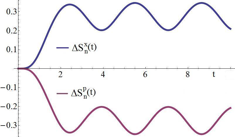
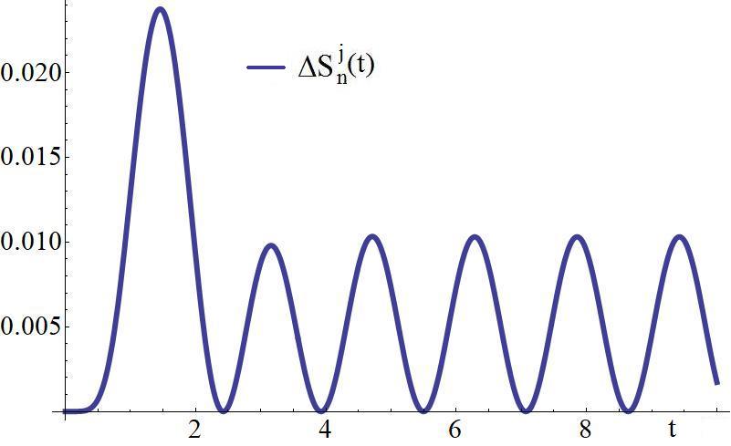
Figure 1: The increase of the position and momentum Shannon entropies as well as the joint entropy corresponding to the choice (2.21) with $a=\epsilon=1$.

Here, we only note that for the frequencies $\omega_{I}(t)$ with the initial conditions (2.17) at $t_{0}=-\infty$ (see eq. (2.26) for the function $b(t)$) we obtain that $S^{x}_{n}(-\infty)=S_{n}^{x}(\infty)$ and analogously for other entropies; in other words the final entropies stabilize independently of the history of the evolution (i.e. the parameter $\epsilon$), see Figs. 2 and 3.

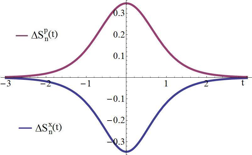
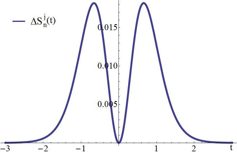
Figure 2: The increase of the position and momentum Shannon entropies as well as the joint entropy corresponding to choice (2.26) with $a=\epsilon=1$.

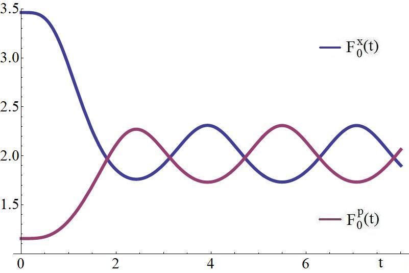
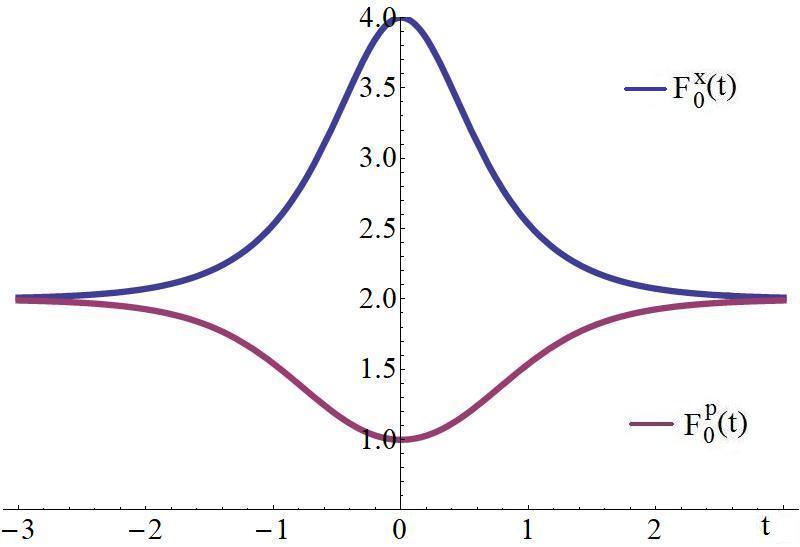
Figure 3: The dynamics of the Fisher information, for $n=0$, corresponding to (2.21) and (2.26), respectively, with $a=\epsilon=1$.

3 Uniform time-dependent magnetic fields

3.1 The dynamics of entropies

Let us consider the Hamiltonian of the charged particle in the electromagnetic field defined by the potentials $\vec{A}$ and $\Phi$

$$H=\frac{1}{2}(\vec{p}-\vec{A})^{2}+\Phi,$$ (3.1)

(for simplicity we put $e=1$ and $m=1$). Then the Schrödinger equation corresponding to the above Hamiltonian (with the potential in the Coulomb gauge) takes the form

$$i\partial_{t}\phi=-\frac{1}{2}\triangle\phi+i(\vec{A}\cdot\vec{\nabla})\phi+\frac{1}{2}\vec{A}^{2}\phi+\Phi\phi.$$ (3.2)

The case of the uniform and constant magnetic field corresponds to the famous Landau levels. When we want to relax that assumption and consider a uniform but time-varying magnetic field $\vec{B}(\vec{x},t)=2\omega(t)\vec{e}_{3}$ the situation complicates, since due to the Faraday law we have also (in general) a time-dependent electric field $\vec{E}(\vec{x},t)=-\dot{\omega}(t)|{\bf{x}}|\vec{e}_{\theta}$. However, in terms of potentials the situation can be described in a similar way as in the constant case

$$\vec{A}(\vec{x},t)=({\bf A}({\bf{x}},t),0)=(-\omega(t)x^{2},\omega(t)x^{1},0),\quad\Phi=0,$$ (3.3)

where the bold letters denote the two-dimensional vectors with the indices $1,2$. Substituting the potential (3.3) into (3.2) we get that the third coordinate decouples and the relevant dynamics is described by the equation

$$i\partial_{t}\phi({\bf{x}},t)=-\frac{1}{2}{\bf\triangle}\phi({\bf{x}},t)+\frac{1}{2}\omega^{2}(t){\bf{x}}^{2}\phi({\bf{x}},t)+\frac{p_{3}^{2}}{2}\phi({\bf{x}},t)-i\omega(t)(x^{2}\partial_{1}-x^{1}\partial_{2})\phi({\bf{x}},t),$$ (3.4)

where $p_{3}$ is the conserved momentum related to the decoupling constant. The wave functions which form a basis of the solutions of eq. (3.4) have been obtained, through the polar coordinates, in Ref. [24]. However, for such a choice of basis it is difficult, in general, to analyse their entropic properties; this is possible only for the ground state [24]. Here we apply a slightly different approach which enables us to extend these considerations to an orthonormal basis of states as well to construct the time-independent Fisher-Shannon complexities. Namely, by means of the time-depended unitary transformation

$$\psi({\bf{x}},t)=e^{it\frac{p_{3}^{2}}{2}}\phi(R(t){\bf{x}},t),\quad R(t)=\left(\begin{array}[]{cc}\cos(\Omega(t))&\sin(\Omega(t))\\ -\sin(\Omega(t))&\cos(\Omega(t))\end{array}\right),$$ (3.5)

where $\dot{\Omega}(t)=\omega(t)$, we reduce eq. (3.4) to the following one

$$i\partial_{t}\psi({\bf{x}},t)=-\frac{1}{2}{\bf\triangle}\psi({\bf{x}},t)+\frac{1}{2}\omega^{2}(t){\bf{x}}^{2}\psi({\bf{x}},t).$$ (3.6)

Thus, the wave functions

$$\phi_{mn}({\bf{x}},t)=e^{-it\frac{p_{3}^{2}}{2}}\psi_{m}(x^{1}\cos(\Omega(t))-x^{2}\sin(\Omega(t)))\psi_{n}(x^{1}\sin(\Omega(t))+x^{2}\cos(\Omega(t))),$$ (3.7)

where $\psi$’s are given by eq. (2.13) form an orthonormal basis for the solutions of the transversal Schrödinger equation (3.4).

Now, imposing on the function $b(t)$ the initial conditions (2.17), we compute the change of the two-dimensional Shannon entropies $S_{m,n}^{{\bf{x}}}$ and $S_{m,n}^{{\bf{p}}}$ of the states (3.7). First, using the fact that $\det(R(t))=1$, after some computations, we find the increase of entropy (from $t_{0}$ to $t$) is of the form

$$\triangle S_{m,n}^{{\bf{x}}}(t)=2\ln(b(t)).$$ (3.8)

Moreover, performing the Fourier transform of the states (3.7), we obtain the momentum density $\rho_{m,n}({\bf{p}},t)$ expressed as the product of the functions (2.41) with the arguments $R^{T}(t){\bf p}$. However, using again the condition $\det(R(t))=1$ we obtain that

$$\Delta S_{m,n}^{{\bf{p}}}(t)=\ln\left(\frac{\omega_{0}^{2}+b^{2}(t)\dot{b}^{2}(t)}{\omega_{0}^{2}b^{2}(t)}\right),$$ (3.9)

where $\omega_{0}=B(t_{0})/2$. Furthermore, we can also find the Fisher information for the discussed basis

$$F_{m,n}^{{\bf{x}}}(t)=\frac{4\omega_{0}}{b^{2}(t)}(m+n+1),\qquad F_{m,n}^{{\bf{p}}}(t)=\frac{4b^{2}(t)\omega_{0}}{\omega_{0}^{2}+b^{2}(t)\dot{b}^{2}(t)}(m+n+1).$$ (3.10)

Let us note that for $m=n=0$ the above results coincide with the ones obtained in Ref. [24]. Finally, the time-independent Fisher-Shannon complexities can be also constructed (cf. eqs. (2.53))

$$F^{{\bf{x}}}_{m,n}(t)e^{S_{m,n}^{{\bf{x}}}(t)}=F^{{\bf{x}}}_{m,n}(t_{0})e^{S_{m,n}^{{\bf{x}}}(t_{0})},\quad F^{{\bf{p}}}_{m,n}(t)e^{S_{m,n}^{{\bf{p}}}(t)}=F^{{\bf{p}}}_{m,n}(t_{0})e^{S_{m,n}^{{\bf{p}}}(t_{0})}.$$ (3.11)

In view of the above results we see that in order to analyse entropic relations for charged particle in the time-varying electromagnetic field (3.3), the explicit form the function $b(t)$ is needed. Such a situation appears for the electromagnetic potential defined by $\omega(t)$ given by $\omega_{II}$ (or $\omega_{I}$ with $a=0$), see (2.28) (and (2.20)). Then, we have electromagnetic pulses (with the uniform magnetic field) which disappear at plus/minus infinity. Since for such a choice of the electromagnetic pulses the function $b(t)$ is an elementary one, see Sec. 2.2, thus we immediately obtain the explicit time dependence of the discussed properties of the entropy; for illustration see Fig. 4, where we present the results for the electromagnetic pulse defined by the frequency (2.28).

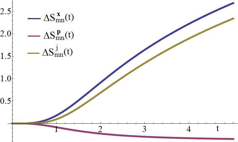
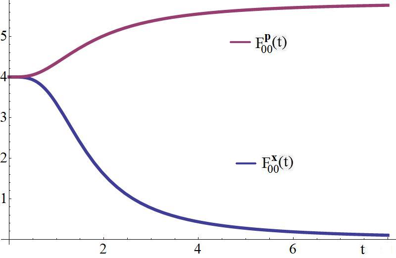
Figure 4: The increase of the position, momentum Shannon entropies and joint entropy as well as the dynamics of the Fisher information for the electromagnetic field (3.3) defined by (2.28) with $a=\epsilon=1$

It is also worth to notice that putting $a\sim\epsilon$ in $\omega_{II}(t)$ and next taking the limit $\epsilon\rightarrow 0$ one obtains the Dirac delta behavior of the magnetic field $\vec{B}(t)\sim\delta(t)\vec{e}_{3}$ . Finally, we will see in the next section that the electromagnetic field defined by $\omega_{II}(t)$ has a nice geometric interpretation.

3.2 Geometric analysis

In the previous section we have seen that for the electromagnetic field defined by $\omega_{II}(t)$ the description of the quantum dynamics of the charged particle simplifies. To better understand this situation we come back to the classical level where as we will show below such a choice has a nice geometric interpretation. To this end let us recall that the classical dynamics of the particle governed by the electromagnetic potential $\vec{A}(\vec{x},t)$ can be embedded, by means of the so-called Eisenhart-Duval lift [25]-[29], into the geodesic equation of the five-dimensional spacetime

$$g=2dtdv+2dt\vec{A}(\vec{x},t)\cdot d\vec{x}+d\vec{x}^{2}.$$ (3.12)

Namely, the geodesic equations corresponding to the $\vec{x}$ coordinates reproduce the Lorentz equations with $\vec{B}$ and $\vec{E}$ determined by $\vec{A}$; equation for the $v$ coordinate decouples while $u$ is proportional to the affine parameter. For the potential given by eq. (3.3) one arrives at the four-dimensional metric

$$g=2dtdv+2\omega(t)(x^{1}dx^{2}-x^{2}dx^{1})dt+d{\bf{x}}^{2},$$ (3.13)

for which only the one component of the Ricci tensor is non-zero, i.e. $R_{tt}(t)=(B^{3})^{2}(t)/2=2\omega^{2}(t)$ (the metric has vanishing the scalar curvature and describes a null-fluid solution to the Einstein equations). Let us now analyse the conformal Killing vectors of the metric (3.13). Of course, one can write out the suitable equations describing the conformal fields. However, a more simpler way is based on the following change of the coordinates

$${\bf{x}}=R(t)\tilde{\bf{x}},$$ (3.14)

where $R(t)$ is given by (3.5). Then, in the new coordinates, the metric takes the form

$$g=2dtdv-\omega^{2}(t)\tilde{\bf{x}}^{2}dt^{2}+d\tilde{\bf{x}}^{2},$$ (3.15)

i.e. it is a conformally flat pp-waves [50]. In consequence, for any function $\omega(t)$ the Lie algebra of the conformal Killing vectors of the metric $g$ is 15-dimensional; however, the number of Killing, homothetic and proper conformal fields depends on the choice of $\omega(t)$. Now let us recall that for the null geodesics the conformal fields yield constants of motion $J=Y_{\mu}\frac{dx^{\mu}}{d\tau}$ which, in turn, in the generic case (i.e. for the so-called chronoprojective fields) can be projected onto constants of motion of the considered classical dynamics (since the classical dynamics is embedded into the geodesic equation); for more details and further references concerning this topic see [25]-[29]. Using the results of Ref. [51] we verify that the field

$$Y=F(t)\partial_{u}-\frac{1}{4}\overset{..}{F}(t)\tilde{{\bf{x}}}^{2}\partial_{v}+\frac{1}{2}\dot{F}(t)\tilde{\bf{x}}\partial_{\tilde{\bf{x}}},$$ (3.16)

where $F(t)$ satisfies equation $\overset{...}{F}(t)+4\dot{\omega}(t)\omega(t)F(t)+4\omega^{2}(t)\dot{F}(t)=0$, is a conformal vector field of the metric (3.15) with the conformal factor $f=\dot{F}/2$. Then, the three independent solutions are: $F(t)=b^{2}(t)$, $F(t)=b^{2}(t)\sin(c\tau(t))$ and $F(t)=b^{2}(t)\cos(c\tau(t))$ where $b(t)$ satisfies the EMP equation (2.3) and $\tau(t)$ is given by (2.6). Now, returning to the initial variable ${\bf{x}}$ the conformal factor remains unchanged but $Y$ takes the form

$$Y=F(t)\partial_{u}-\frac{1}{4}\overset{..}{F}(t){{\bf{x}}}^{2}\partial_{v}+\frac{1}{2}\dot{F}(t){\bf{x}}\partial_{{\bf{x}}}-\omega(t)F(t)(x^{1}\partial_{2}-x^{2}\partial_{1}).$$ (3.17)

The field (3.17) implies the integral of motion (for null geodesics) of the from

$$J=F(t)\dot{v}-\frac{1}{4}\overset{..}{F}(t){{\bf{x}}}^{2}-F(t){\bf A}^{2}({\bf{x}},t)+\frac{1}{2}\dot{F}(t){\bf{x}}\cdot\dot{\bf{x}}.$$ (3.18)

On the other hand, by virtue of the null condition of the geodesic one has $\dot{v}=-\frac{1}{2}\dot{\bf{x}}^{2}-{\bf A}\cdot\dot{\bf{x}}$. In consequence, the constant of motion $J$ can be projected onto the integral of motion of the initial dynamics, i.e. the Lorentz equation for the electromagnetic field defined by (3.3); namely, we have

$$J=-\frac{1}{2}F(t)\dot{\bf{x}}^{2}-\frac{1}{4}\overset{..}{F}(t){{\bf{x}}}^{2}-F(t){\bf A}^{2}({\bf{x}},t)+\left(\frac{1}{2}\dot{F}(t){\bf{x}}-F(t){\bf A}({\bf{x}},t)\right)\cdot\dot{\bf{x}};$$ (3.19)

now, $J$ depends on $t$ and ${\bf{x}}$ only.

Next, let us take the conformal field generated by $F(t)=b^{2}(t)$, where $b(t)$ satisfies eq. (2.3). Then the conformal factor is of the form $f(t)=b(t)\dot{b}(t)$ and the corresponding integral of motion takes the form

$$J=-\frac{1}{2}b^{2}(t)\dot{\bf{x}}^{2}-\frac{1}{2}\left(\omega^{2}b^{2}(t)+\dot{b}^{2}(t)+\frac{c^{2}}{b^{2}(t)}\right){\bf{x}}^{2}+(b(t)\dot{b}(t){\bf{x}}-b^{2}(t){\bf A}({\bf{x}},t))\dot{\bf{x}}.$$ (3.20)

In order to make the meaning of $J$ more transparent let us note that it can be rewritten in the following form

$$J=-\frac{1}{2}\left((b(t){\bf p}-\dot{b}(t){\bf{x}})^{2}+\frac{c^{2}{\bf{x}}^{2}}{b^{2}(t)}\right),$$ (3.21)

where ${\bf p}$ is the canonical momentum, i.e. ${\bf p}=\dot{\bf x}+{\bf A}$. In summary, the integral of motion associated with such a conformal field corresponds to the Ermakov-Lewis invariant (cf. eq. (2.15)); however, we should keep in mind that it contains the canonical momenta (not the kinetic ones).

Now, let us recall [50] that among all proper conformal vectors the most interesting seem the so-called special ones, i.e. when the conformal factor $f$ satisfies $\textrm{Hess}(f)=0$ (such a condition holds, for example, for any conformal field of the Minkowski spacetime or even any vacuum solution to the Einstein equations). Following Ref. [50] we have that the metric given by (3.15) admit a special conformal Killing vector if and only if $\omega(t)=\omega_{II}(t)$. Moreover, taking into account the above considerations this holds only for the conformal Killing field (3.16) defined by

$$F(t)=b^{2}(t)=t^{2}+\epsilon^{2}.$$ (3.22)

In this case the conformal factor is $f(t)=t$ and $b(t)$ satisfies the EMP equation (2.3) with $c^{2}=a^{2}+\epsilon^{2}$. In view of this and the considerations presented in Sec. 2.1 (see the transformation (2.8)) as well as eq. (3.14) we immediately obtain the explicit solvability of the Lorentz equation with the potential (3.3) defined by $\omega(t)=\omega_{II}(t)$. Finally, the integral of motion $J$, defined by (3.21), in terms of ${\bf y},\tau$ variables corresponds to the energy of the two-dimensional, isotopic, harmonic oscillator with the frequency $c^{2}=a^{2}+\epsilon^{2}$.

4 Time dependent coupled oscillators

4.1 Entanglement dynamics of coupled oscillators

The aim of the present section is to show that the results of Sec. 2.2 can be also useful in the analysis of the entanglement entropy for the system of two harmonic (in general with time-dependent frequencies) oscillators coupled by a time-dependent parameter. More precisely, let us consider the Hamiltonian of the form

$$H(t)=\frac{1}{2}(p_{1}^{2}+p_{2}^{2})+\frac{1}{2}\omega^{2}(t)\left((x^{1})^{2}+(x^{2})^{2}\right)+\frac{1}{2}k(t)\left(x^{1}-x^{2}\right)^{2}.$$ (4.1)

Then the transformation ${\bf x}=R{\bf y}$ where $R$ is given by (3.5) with $\Omega(t)=\pi/4$ transforms the Hamiltonian (4.1) into the following one

$$H_{\bf y}(t)=\frac{1}{2}(p_{1}^{2}+p_{2}^{2})+\frac{1}{2}\left(\omega^{2}_{1}(t)(y^{1})^{2}+\omega^{2}_{2}(t)(y^{2})^{2}\right),$$ (4.2)

where now $p$’s denote the canonical momenta associated with $y$’s and $\omega_{1}^{2}(t)=\omega^{2}(t)+2k(t),\quad\omega_{2}^{2}(t)=\omega^{2}(t)$. The frequencies $\omega_{1,2}(t)$ determine the parameters of the initial Hamiltonian (4.1) as follows

$$\omega(t)=\omega_{2}(t),\quad k(t)=\frac{1}{2}(\omega_{1}^{2}(t)-\omega_{2}^{2}(t)).$$ (4.3)

The evolution $\psi_{0}({\bf{x}},t)$ of the ground state $\psi_{0}({\bf{x}},t_{0})$ of the Hamiltonian operator $\hat{H}(t_{0})$ as well as the reduced density matrix $\rho_{0,red}(x^{1},\tilde{x}^{1},t)=\int\psi_{0}(x^{1},x^{2},t)\psi^{*}_{0}(\tilde{x}^{1},x^{2},t)dx_{2}$ can be easily computed when we take into account the form of the Hamiltonian (4.2) and next return to the ${\bf{x}}$ variable. The final results is of the form (see [30])

$$\rho_{0,red}(x^{1},\tilde{x}^{1},t)=\frac{1}{\sqrt{\pi(\zeta(t)-\chi(t))}}e^{\chi(t)x^{1}\tilde{x}^{1}+i((x^{1})^{2}-(\tilde{x}^{1})^{2})\varphi(t)-\frac{\zeta(t)}{2}((x^{1})^{2}+(\tilde{x}^{1})^{2})},$$ (4.4)

where

$$\varphi(t)=\frac{\dot{b}_{1}(t)}{4b_{1}(t)}+\frac{\dot{b}_{2}(t)}{4b_{2}(t)}-\frac{\frac{c_{1}}{b_{1}^{2}(t)}-\frac{c_{2}}{b_{2}^{2}(t)}}{\frac{c_{1}}{b_{1}^{2}(t)}+\frac{c_{2}}{b_{2}^{2}(t)}}\left(\frac{\dot{b}_{1}(t)}{4b_{1}(t)}-\frac{\dot{b}_{2}(t)}{4b_{2}(t)}\right),$$ (4.5)

and $\zeta(t)>\chi(t)\geq 0$ are given by

$$\zeta(t)=\frac{\left(\frac{c_{1}}{b_{1}^{2}(t)}+\frac{c_{2}}{b_{2}^{2}(t)}\right)^{2}+4\frac{c_{1}c_{2}}{b_{1}^{2}(t)b_{2}^{2}(t)}+\left(\frac{\dot{b}_{1}(t)}{b_{1}^{2}(t)}-\frac{\dot{b}_{2}(t)}{b_{2}^{2}(t)}\right)^{2}}{4\left(\frac{c_{1}}{b_{1}^{2}(t)}+\frac{c_{2}}{b_{2}^{2}(t)}\right)},\quad\chi(t)=\frac{\left(\frac{c_{1}}{b_{1}^{2}(t)}-\frac{c_{2}}{b_{2}^{2}(t)}\right)^{2}+\left(\frac{\dot{b}_{1}(t)}{b_{1}^{2}(t)}-\frac{\dot{b}_{2}(t)}{b_{2}^{2}(t)}\right)^{2}}{4\left(\frac{c_{1}}{b_{1}^{2}(t)}+\frac{c_{2}}{b_{2}^{2}(t)}\right)},$$ (4.6)

while the functions $b_{1,2}(t)$ satisfy the EMP equation (2.3) with the frequencies $\omega_{1,2}(t)$ and the constants $c_{1}=\sqrt{\omega^{2}(t_{0})+2k(t_{0})}$ and $c_{2}=\omega(t_{0})$, respectively. Then the Rényi entropy $R^{\alpha}(t)=\ln(\textrm{tr}(\rho_{0,red}^{\alpha}))/(1-\alpha)$ and the von Neumann entropy $S=\lim_{\alpha\rightarrow 1}R^{\alpha}$ of the reduced density $\rho_{0,red}$ can be computed, see Ref. [30] (see also [52])

$$R^{\alpha}(t)=\frac{1}{1-\alpha}\ln\frac{(1-\xi(t))^{\alpha}}{1-\xi(t)},\quad S(t)=-\ln(1-\xi(t))-\frac{\xi(t)}{1-\xi(t)}\ln\xi(t),$$ (4.7)

where $\xi(t)=\frac{\chi(t)}{\zeta(t)+\sqrt{\zeta^{2}(t)-\chi^{2}(t)}}$. In view of the above formulae we see that the entanglement entropy is directly determined by the solutions of the two EMP equations with the frequencies $\omega_{1,2}(t)$.

Eqs. (4.6) and (4.7) enable us to analyse directly the dynamics of various entropies provided we have explicit solutions to the EMP equation. Such a situation holds for abrupt profiles and it was presented in Refs. [30, 54]; here, we complete these results by considering examples with the continuously changing parameters; in particular, the ones for which the entropy stabilizes. To this end, we use the exact examples presented in Sec. 2.2 to describe dynamics of the entropies for different forms of the coupling $k(t)$ and frequency $\omega(t)$ appearing in the Hamiltonian (4.1). Namely, taking $\omega_{2}^{2}(t)=\omega_{2}^{2}=const<a^{2}$ (thus $b_{2}(t)=1$) and $\omega_{1}(t)=\tilde{\omega}_{I}(t)$ (with $\tilde{b}_{1}(t)$ given by eq. (2.25)), by virtue of (4.3), we obtain the two harmonic oscillators both with the frequency $\omega_{2}$ coupled by the decreasing (quenched) function $k_{1}(t)$, for which the values start at $(2/\epsilon^{2}+a^{2}-\omega_{2}^{2})/2$ and end at $(a^{2}-\omega_{2}^{2})/2$ (see Fig. 5a). A similar situation holds when we take $\omega_{2}(t)=\omega_{2}=const<a/\epsilon^{2}$ and $\omega_{1}(t)=\tilde{\tilde{\omega}}_{II}(t)$ with $t_{0}=0$. Another example is given by $\omega_{1}(t)=\omega_{I}(t)$ and the initial condition at $t_{0}=-\infty$; then we obtain again the two harmonic oscillators coupled by the parameter $k_{2}(t)$; however this time the coupling starts and ends at $(a^{2}-\omega_{2}^{2})/2$ at minus/plus infinity and attains the maximal value at $t=0$ (see Fig. 5b). Let us stress that in this case for the function $b_{1}(t)$ we have $b_{1}(-\infty)=b_{1}(\infty)$ (see eq. (2.26)) thus the final value of the entanglement entropy (see eqs. (4.7) and (4.6)) stabilizes (there is no oscillatory behavior at $t=\infty$) and it is equal to the initial one (see also Fig. 5b). Such a situation is quite different from the generic oscillatory behavior, cf. [30, 54]; moreover, it holds independently of the history of evolution (i.e. the parameter $\epsilon$).

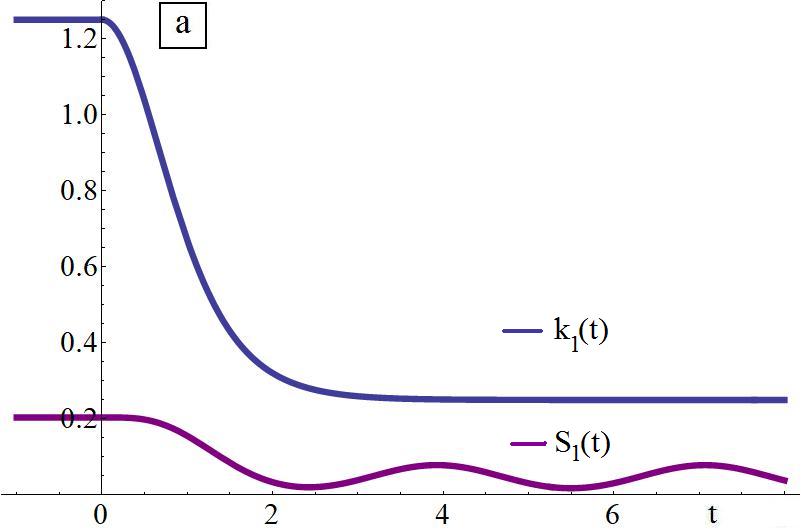
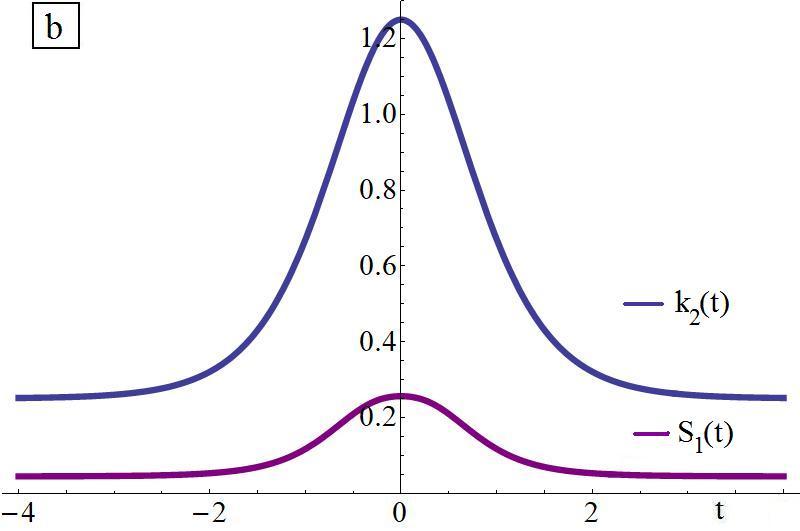
Figure 5: The coupling parameter and the corresponding entanglement entropy a) $k_{1}(t)$ b) $k_{2}(t)$, $a=\epsilon=1,\ \omega_{2}^{2}=1/2$.

Of course, one can take other combinations of frequencies $\omega$’s presented in Sec. 2.2 to obtain various forms of the time-dependent harmonic oscillators coupled by time-dependent parameters; for example taking $\omega_{1}(t)=\omega_{II}(t)$ and $\omega_{2}(t)=\omega_{I}(t)$ both with the parameter $\epsilon=1$ (implying $k\geq 0$) or changing the the values $a,\epsilon$ of the frequencies. More generally, those frequencies can be directly applied to the Wigner distribution functions, entropies or uncertainty relations of many integrating time-dependent harmonic oscillators where more functions $b(t)$’s are involved (also for excited states), see [53]-[58] for more details.

4.2 Quantum decoherence

One of the outstanding features of the quantum mechanics is the superposition principle. However, this feature is very fragile and its loss can lead to many problems, in particular the ones related to quantum computations and computers (e.g. construction of quantum memory). Usually the loss of quantum coherence, or, in general, the occurrence of the quantum-classical transition, is related to the dissipative interaction of the system with the environment. In consequence, such problems are quite complicated and involve the framework of the quantum open systems (such as master equation) [31, 32]. Moreover, various, inequivalent, measurements of decoherence (classicality) have been proposed; the main ones are based on the off-diagonal elements of the density matrix. Let us have a look on these issues in the context of the results obtained in previous sections.

First, let us recall that for the density matrix $\rho(x,\tilde{x},t)$ in the Gaussian form a measure of the degree of decoherence (related to the damping of the off-diagonal elements of $\rho$) is given by the following formula

$$\delta_{QD}(t)=\sqrt{\frac{\Gamma_{c}(t)}{\Gamma_{d}(t)}},$$ (4.8)

where $\Gamma$’s are coefficients appearing in the density matrix when it is expressed in terms of the variables $x_{c}=(x+\tilde{x})/2$ and $x_{d}=(x-\tilde{x})/2$, i.e.

$$\rho(x_{c},x_{d},t)=\exp(-\Gamma_{c}(t)x_{c}^{2}-\Gamma_{d}(t)x_{d}^{2}-\Gamma_{e}(t)x_{c}x_{d}+\textrm{linear terms}).$$ (4.9)

On the other hand, there is a second, independent, measure of the classicality of the quantum system; namely, the classical correlation $\delta_{CC}$ which measures the sharpness ($\delta_{CC}\ll 1$) of the Wigner function around the classical trajectory; for the density matrix (4.9) it is given by

$$\delta_{CC}(t)=\frac{\sqrt{\Gamma_{c}(t)\Gamma_{d}(t)}}{|\Gamma_{e}(t)|}.$$ (4.10)

For more details concerning $\delta_{QD}$ and $\delta_{CC}$ we refer to Refs. [31, 33, 34]; here we only note that $\delta_{QD}$ can be expressed by the purity of $\rho$, i.e. $\delta_{QD}=\textrm{tr}(\rho^{2})$ (thus $\delta_{QD}\leq 1$ and it is representation invariant), while $\delta_{CC}$ is a dimensionless quantity.

To begin with, let us apply the above measures to the TDHO (2.1). For the state $\psi_{n}$, see (2.13), with $n=0$ we obtain

$$\delta_{QD}^{0}(t)=1,\quad\delta_{CC}^{0}(t)=\frac{c}{2b(t)\dot{b}(t)}.$$ (4.11)

Thus there is no quantum decoherence, though the entropies change in time (see eqs. (2.43) and (2.44)). In this case the change of the entropy is related to the second measure of the classicality. In fact, by virtue of eq. (2.44) (for $n=0$ and $c=\omega_{0}$) we obtain the following relation between the joint entropy and classical correlation

$$\Delta S_{0}^{j}(t)=\frac{1}{2}\ln\left(1+\frac{1}{4\delta_{CC}^{2}(t)}\right);$$ (4.12)

it can be also easily inverted. For the ordinary harmonic oscillator and ground state ($b(t)=1$) we obtain, as expected, infinite $\delta_{CC}^{0}$ and the constant entropy. For the time-dependent case $\omega(t)$ with the final frequency equal to zero (see eq. (2.23) and (2.36) for abrupt quench) the classical correlation can be arbitrary small for sufficiently large time, while $\delta_{QD}^{0}$ remain unchanged.

According to the general belief the decoherence phenomena appear when a quantum system interacts with some environment [31, 32]. In general, such an approach involves a more complicated analysis. However, in the case of two oscillators coupled to each other the first can be treated as the system under consideration and the second one as the environment; then the reduced density matrix can be used to describe the influence of the surroundings on the system. In view of this let us consider the Hamiltonian given by (4.1). By means of eq. (4.8), or alternatively computing the trace of $\rho^{2}_{0,red}$, we find that

$$\delta_{QD}^{0}(t)=\sqrt{\frac{\zeta(t)-\chi(t)}{\zeta(t)+\chi(t)}}=\frac{1-\xi(t)}{1+\xi(t)}.$$ (4.13)

In view of this the quantum decoherence emerges and it is time-dependent (in contrast to the single, noninteracting, TDHO studied above). In terms of the solutions $b_{1}$ and $b_{2}$ of the EMP equation (4.13) takes the form

$$\delta_{QD}^{0}(t)=\frac{2{\sqrt{c_{1}c_{2}}b_{1}(t)b_{2}(t)}}{\sqrt{(c_{1}b_{2}^{2}(t)+c_{2}b_{1}^{2}(t))^{2}+(\dot{b}_{1}(t)b_{2}(t)-\dot{b}_{2}(t)b_{1}(t))^{2}b_{1}^{2}(t)b_{2}^{2}(t)}}.$$ (4.14)

The formula (4.14) simplifies for two harmonic oscillators coupled by time dependent parameter $k(t)$ (since $b_{2}(t)=1$); then we can simply use the examples discussed in Sec. 4.1 to analytically analyse the degree of quantum decoherence. In the simplest case of two harmonic oscillators coupled by a constant parameter, $\delta_{QD}^{0}$ reduces to a constant which coincides with observation made in Ref. [59]. Finally, it is also worth to notice that the relation (4.13) can be inverted $\xi(t)=(1-\delta_{QD}^{0}(t))/(1+\delta_{QD}^{0}(t))$ and then various entropies (see eqs. (4.7)) can be expressed in terms of quantum decoherence.

For the second measure, i.e. the classical correlation, we get

$$\delta_{CC}^{0}(t)=\frac{\sqrt{\zeta^{2}(t)-\chi^{2}(t)}}{4|\varphi(t)|},$$ (4.15)

where $\zeta(t),\chi(t)$ and $\varphi(t)$ are given by eqs. (4.5) and (4.6). For the the harmonic oscillators and constant coupling $\delta_{CC}^{0}(t)$ is infinite; this is in contrast with the time-dependent case where it is usually finite, enhancing in this way the classicality of the system (this can be again easily seen using the results presented in Sec. 4.1). These considerations suggest that the time-dependent coupling (interaction) of the system with environment can lead to more serious destruction of quantum properties.

To conclude our investigations let us note that the above results can be also useful in other models and thus in further studies of the decoherence phenomena. To this end let us consider the TDHO driven by an external time-dependent force, i.e.

$$\overset{..}{x}(t)=-\omega^{2}(t)x(t)+f(t).$$ (4.16)

It turns out that the quantum counterpart of (4.16) can be reduced to the force-free case [60]. Namely, the solution of the Schrödinger equation corresponding to (4.16) is of the form

$$\phi(x,t)=\psi(x-e(t),t)e^{i\dot{e}(t)(x-e(t))+i\int Ldt},$$ (4.17)

where $\psi$ is a solution of the force-free Schrödinger equation, $L$ is the classical Lagrangian for eq. (4.16) and $e(t)$ is a solution to the classical equation of motion (4.16). In view of this the frequencies $\omega(t)$ for which explicit solutions of the TDHO are known (see Sec. 2) can be also very useful when $f$ is not equal to zero. Such a situation appears, for example, in the study of the entropies and measures of the classicality mentioned above.

In fact, by means of eq. (4.17) we find, after straightforward calculations, that all entropies $S^{x}$, $S^{p}$ and $S^{j}$ reduce to the ones for the force-free case (in particular they are described by the function $b(t)$ for the states $\phi_{n}$ corresponding to $\psi_{n}$ defined in Sec. 2). Moreover, the $\delta_{QD}^{0}$ and $\delta_{CC}^{0}$ for $\phi_{0}$ are given also by (4.11) for the TDHO with an arbitrary driven force; in consequence, the relation (4.12) remains valid and there is no decoherence. However, the discussed driving model (4.16) has an interesting modification when the external force change randomly [61]. Then even in the case of the harmonic oscillator the joint entropy changes in time [22]; this suggests that for a random driving force $\delta_{QD}^{0}$ can also change with time; however, this involves more careful analysis of the ensemble average of the density matrix.

5 A quantum quench for non-relativistic fermions

One of the examples of basic phenomena where the TDHO can be useful are the ones related to non-equilibrium processes for which time-dependent parameters appear. Such systems are modeled by quantum fields subjected to a quench. It turns out that in the relativistic theory some universal phenomena emerge for the (a)diabatic regime; for example,the Kibble-Zurek scaling, for review see [62]. On the other hand, from the experimental point of view the non-relativistic theories are also interesting. In consequence, the question arises whether a similar behavior emerges for non-relativistic systems. Such a problem has been recently discussed in Ref. [44] for the system of many mutually non-interacting non-relativistic fermions in a harmonic trap (important in the context of cold atom physics). In particular, it has been shown that the description of the dynamics of basic quantities for such a system is related to the EMP equation (2.3); for example, for the expectation value $\langle\hat{O}\rangle(t)$ of the operator

$$\hat{O}(t)=\int x^{2}\hat{\Psi}(x,t)^{\dagger}\hat{\Psi}(x,t)dx,$$ (5.1)

between the ground ”in” states (defined at early times) we have

$$\langle\hat{O}\rangle(t)\sim b^{2}(t).$$ (5.2)

Furthermore, the entanglement entropy in a given finite subregion for large number of fermions can be also related to $b(t)$, it is proportional to the area of the region and $b^{-1}(t)$ (for more details we refer to [44], in particular see formulae 3.8 and 7.8 therein).

A typical situation is when the initial Hamiltonian is gapped, while the frequency crosses or approaches a critical point where the gap vanishes. The last possibility, where the initial frequency decreases to zero at late times (release from the harmonic trap) is called the ending protocol. Such a protocol has been analysed in Ref. [44] by means of $\omega^{2}(t)\sim 1-\tanh(t)$. However, for such a choice the general solution of the EMP equation (2.3) is a quite complicated special function; in consequence, the analysis of (a)diabatic regions quite involved. In contrast, for the quenched protocol modeled by the frequency (2.24) with $a=0$ or (2.34) with $t_{0}=0$, the function $b(t)$ is an elementary one and thus the (a)diabtic analysis of the expectation value (5.2) as well as the estimation of the entanglement entropy of a subregion become more accessible. Let us see this in more detail.

In order to control both the slow and fast quenches in the neighborhood of the critical point and to include the instantaneous quench, see eq. (2.36), we will use $\tilde{\omega}_{II}(t)$ with $a=\alpha\epsilon^{2}$ and $t_{0}=0$. Then the function $b(t)$ for $t\geq 0$ can be expressed as follows

$$b^{2}(s)=\frac{s^{2}+1}{2(1+\beta^{2})}(\cos(2\sqrt{1+\beta^{2}}\tan^{-1}(s))+1+2\beta^{2}),$$ (5.3)

where $s=t/\epsilon$ and $\beta=\alpha\epsilon$. Since the frequency $\tilde{\omega}_{II}(t)$ approaches the critical point at plus infinity, the adiabaticity breaks down at some time $t_{c}$ (the so-called Kibble-Zurek time). In our case the Landau criterion

$$\frac{|\dot{\omega}(t)|}{\omega^{2}(t)}\sim 1,$$ (5.4)

implies $t_{c}\sim\alpha\epsilon^{2}/2$, thus we put $s_{c}=\beta$. On the other hand, the adiabatic approximation $b_{ad}^{2}(t)=\omega_{0}/\omega(t)$ yields

$$b_{ad}^{2}(s)=1+s^{2}.$$ (5.5)

In consequence, by virtue of (5.2) we obtain the approximative relation $\langle\hat{O}\rangle(s_{c})\sim b_{ad}^{2}(s_{c})=1+\beta^{2}\sim\beta^{2}$ (in the slow regime $\beta\gg 1$). This result can be easily refinement by substituting $s=s_{c}=\beta$ into eq. (5.3)

$$b^{2}(s_{c})=\beta^{2}+\cos^{2}(\sqrt{1+\beta^{2}}\tan^{-1}(\beta)).$$ (5.6)

Thus there is an additional term which only for $\beta\gg 1$ (slow regime) can be skipped and then the scaling is consistent with the Kibble-Zurek argument.

In general, the difference between the adiabatic solution $b_{ad}^{2}(s)$ and the exact one is of the form

$$\Delta b^{2}(s)\equiv b_{ad}^{2}(s)-b^{2}(s)=\frac{s^{2}+1}{1+\beta^{2}}\sin^{2}(\sqrt{1+\beta^{2}}\tan^{-1}(s)).$$ (5.7)

From eq. (5.7) follows that for a sufficiently large value of $\beta$ (i.e. $\beta^{2}>3$) the function $\Delta b^{2}(s)$ vanishes at some initial points (for larger $\beta$ we have more points) and thus $b(s)$ is close to the adiabatic solution; for large value of $s$ ($s\gg s_{c}$) the function $\Delta b^{2}(s)$ increases to infinity (see also Fig. 6a). However, for special values, i.e. $\beta=\sqrt{4k^{2}-1}$ where $k\in{\mathbb{N}}$, we have $\lim_{s\rightarrow\infty}\Delta b^{2}(s)=1$. In particular, for $k=1$ ($\beta=\sqrt{3}$) we have that

$$\Delta b^{2}(s)=\frac{s^{2}}{1+s^{2}},$$ (5.8)

thus $0\leq\Delta b^{2}(s)<1$; despite a quite small value of the parameter $\beta$ the distance from the adiabatic solution remains bounded for all times (see also Fig. 6b for $k=2$, i.e. $\beta=\sqrt{15}$).

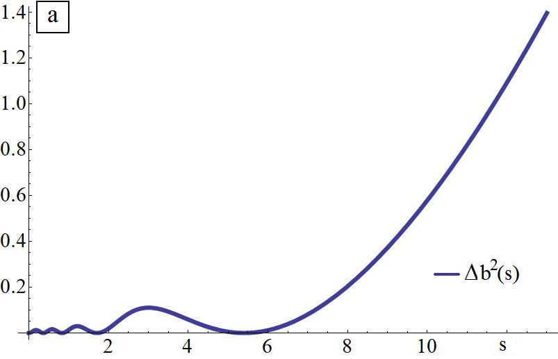
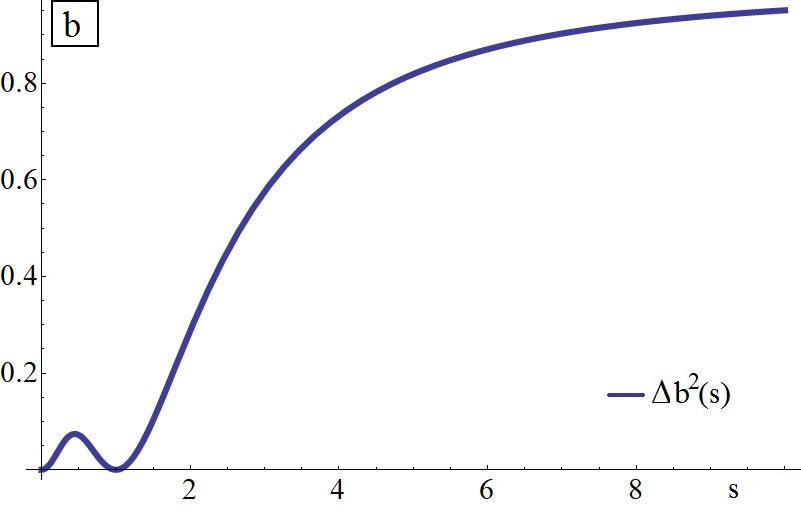
Figure 6: The function $\Delta b^{2}(s)$ a) for $\beta=9$, b) for $\beta=\sqrt{15}$

Now, let us have a look on the fast regime and late times. More precisely, we assume that $\beta\ll 1$ and $t\gg\beta$ (equivalently $s\gg 1$). Then expanding (5.3) with respect to $s$ we have

$$b^{2}(s)=\frac{1}{2\lambda^{2}}\left(s^{2}(2\lambda^{2}+\cos(\pi\lambda)-1)+2s\lambda\sin(\lambda\pi)+(2\lambda^{2}-1)(1-\cos(\lambda\pi))+O(\frac{1}{s})\right).$$ (5.9)

Now, taking into account that $\lambda^{2}=1+\beta^{2}$ and expanding eq. (5.9) up to $\beta^{2}$ we have

$$b^{2}(s)\simeq s^{2}\beta^{2}-s\frac{\pi\beta^{2}}{2}+\beta^{2}+1+O(1/s)\equiv\alpha^{2}t^{2}+1-t\frac{\pi\alpha^{2}\epsilon}{2}+\alpha^{2}\epsilon^{2}+O(1/t).$$ (5.10)

Comparing it with eq. (2.36), we see that the two last terms of (5.10) describe corrections to the abrupt quench for which the frequency suddenly changes from $\alpha$ to zero.

In summary, using $\tilde{\omega}_{II}(t)$ we can simplify the analysis of quenched processes which exhibit critical points. In consequence, some basic quantities, such as expectation values and the entanglement entropy of a finite subregion for large number of fermions takes a more accessible form.

6 Summary and outlook

In this work we have analysed dynamical aspects of information-theoretic and entropic properties of various time-dependent quantum systems. We started with the harmonic oscillator with the time-dependent frequency. In this case we showed that the increase of the position and momentum Shannon (Rényi) or joint entropies of the states which initially are eigenstates of the instantaneous Hamiltonian depend only on the solution of the EMP equation; the same concerns the dynamics of the Fisher information of those states. These results allowed us to examine the Cramér-Rao inequalities as well to find the explicit relation between the Fisher information and the increase of the Shannon entropy. As a consequence, we found that the Fisher-Shanon complexities are time independent quantities for such a basis. Next, we have shown that a similar situation holds for a suitable choice of the basic wave functions of the charge particle in the uniform and time-dependent magnetic field (supplemented by a electric field).

In order to illustrate the results we considered some examples of frequencies for which the solutions of the EMP equation are elementary ones; in consequence, all the mentioned dynamical relations take immediately the explicit forms. Moreover, by means of the Eisenhart-Duval lift, we showed that some conformal Killing vectors imply the integrals of the (geodesics) motion which, in turn, naturally lead to the Ermakov-Lewis invariants for the considered electromagnetic fields. In particular, we have shown that the existence of the special conformal vector implies solvability for the one of those fields.

Next, we have explicitly worked out the entanglement entropy of the harmonic (in general, with time-dependent frequencies) oscillators coupled by a continuous time-dependent parameter. In particular, we showed that for a special form of the coupling parameter the final value of the entanglement entropy stabilizes (independently of the history of evolution). We also showed that the above results and analytical examples can be useful for the study of the quantum-classical transition. To this end we have examined two independent measures of the classicality and their relation with the entropy; in particular, we considered some aspects of the quantum decoherence which plays the relevant role in quantum information processing (technology).

In the last part of the work we have studied in some detail the behavior of quantum quenches (in the presence of the critical points) for the case of mutually non-interacting non-relativistic fermions in a harmonic trap. In particular, we explicitly analysed the scaling behavior of the basic expectation values in the context of the Kibble-Zurek argument and adiabatic limit. Moreover, the discussed exact solutions of the EMP equation yield direct description of the entanglement entropy of a given subregion for large number of fermions.

The results obtained can serve as a starting point for further considerations. Let us point out a few of them. First, following Sec. 2 we can consider further information-theoretic aspects of quantum systems such as the Tsallis entropy or the LMC shape complexity [63] and/or introduce time-dependent mass. On the other hand, in view of Refs. [30, 55] the examples from Sec. 2.2 can be directly used to illustrate, in the exact analytical form, the time-dependent von Neumann and Rényi entropies for a system of many coupled oscillators, following a continuous quench. Moreover, they can be applied to the Wigner distribution functions and/or anisotropic oscillators [54, 57, 56]. They can be also useful in a more general frameworks of the perturbative theory [64] (note that we can compute the explicit form of propagator for the discussed frequencies). Moreover, it would be interesting to compare the results with the numerical methods based on the so-called Gaussian state approximation (such an approach has been quite recently applied for instantaneous quenches [65]) as well as to analyse the time-dependent case of vanishing frequencies (UV divergences) in the spirit of the work [66]. Finally, note that the considerations from the last section fit perfectly into the recent studies [67] of quantum quenches of the $c=1$ Matrix Model which, in turn, is related to the description of two-dimensional string theory with the time-dependent string coupling.

References

- [1] C. Shannon, W. Weaver, “A Mathematical Theory of Communication” The University of Illinois Press, Urbana, Illinois (1949)
- [2] A. Rényi, “On Measures of Entropy and Information” Proc. Fourth Berkeley Symp. Math. Stat. Probability 1 (1961) 547
- [3] R. Fisher, “Theory of Statistical Estimation” Proc. Cambridge Philos. Soc. 22 (1925) 700
- [4] I. Białynicki-Birula, J. Mycielski, “Uncertainty relations for information entropy in wave mechanics” Commun. Math. Phys. 44 (1975) 129
- [5] P. Sánchez-Moreno, A. Plastino, J. Dehesa, “A quantum uncertainty relation based on Fisher’s information” J. Phys. A: Math. Theor. 44 (2011) 065301
- [6] A. Stam, “Some inequalities satisfied by the quantities of information of Fisher and Shannon” Inf. Control. 2 (1959) 101
- [7] A. Dembo, T. Cover, J. Thomas, “Information theoretic inequalities” IEEE Trans. Inform. Theory 37 (1991) 1501
- [8] C. Vignat, J.-F. Bercher, “Analysis of signals in the Fisher-Shannon information plane” Phys. Lett. A 312 (2003) 27
- [9] J. Angulo, J. Antolín, K. Sen “Fisher-Shannon plane and statistical complexity of atoms” Phys. Lett. A 372 (2008) 670
- [10] N. Sobrino-Coll, D. Puertas-Centeno, I. Toranzo, J. Dehesa, “Complexity measures and uncertainty relations of the high-dimensional harmonic and hydrogenic systems” J. Stat. Mech. (2017) 083102
- [11] R. Horodecki, P. Horodecki, M. Horodecki, K. Horodecki, “Quantum entanglement” Rev. Mod. Phys. 81 (2009) 865
- [12] H. Lewis, “Classical and Quantum Systems with Time-Dependent Harmonic-Oscillator-Type Hamiltonians” Phys. Rev. Lett. 18 (1967) 510
- [13] H. Lewis, W. Riesenfeld “Class of Exact Invariants for Classical and Quantum Time-Dependent Harmonic Oscillators” J. Math. Phys. 10 (1969) 1458
- [14] V. Ermakov, “Second order differential equations. Conditions of complete integrability” Univ. Izv. Kiev, Series III 9 (1880) 1 (English translation: A. Harin, under redaction by P. Leach, Appl. Anal. Discrete Math. 2 (2008) 123)
- [15] E. Milne, “The Numerical Determination of Characteristic Numbers” Phys. Rev. 35 (1930) 863
- [16] E. Pinney, “The nonlinear differential equation ” Proc. Am. Math. Soc. 1 (1950) 681.
- [17] J. Choi, M.-S. Kim, D. Kim , M. Maamache, S. Menouar, I. Nahme, “Information theories for time-dependent harmonic oscillator” Ann. Phys. 326 (2011) 1381
- [18] E. Aktürk, Ö. Özcan, R. Sever, “Joint Entropy of the Harmonic Oscillator with Time Dependent Mass and/or Frequency” Int. J. Mod. Phys. B 23 (2009) 2449
- [19] V. Aguiar, I. Guedes, “Fisher information of quantum damped harmonic oscillators” Phys. Scr. 90 (2015) 045207
- [20] S. Najafizade1, H. Hassanabadi, S. Zarrinkamar, “Theoretical information measurement in nonrelativistic time-dependent approach” Indian. J. Phys. 92 (2018) 183
- [21] V. Aguiar , I. Guedes, “Joint entropy of quantum damped harmonic oscillators” Physica A 401 (2014) 159
- [22] A. Fotue, A. Wirngo, R. Keumo Tsiaze, M. Hounkonnou, “Joint entropy and decoherence without dissipation in a driven harmonic oscillator” Eur. Phys. J. Plus 136 (2016) 131
- [23] V. Aguiar, I. Guedes, I. Pedrosa, “Tsallis, Rényi, and Shannon entropies for time-dependent mesoscopic RLC circuits” PTEP (2015) 113A01
- [24] V. Aguiara, I. Guedes, “Entropy and information of a spinless charged particle in time-varying magnetic fields” J. Math. Phys. 57 (2016) 092103
- [25] G. Burdet, C. Duval, M. Perrin, “Time-dependent quantum systems and chronoprojective geometry” Lett. Math. Phys. 10 (1985) 255
- [26] C. Duval, G. Burdet, H. Kunzle, M. Perrin, “Bargmann structures and Newton-Cartan theory” Phys. Rev. D 31(1985) 1841
- [27] M. Cariglia, G. Gibbons, J.-W. van Holten, P. Horvathy, P.-M. Zhang, “Conformal Killing Tensors and covariant Hamiltonian Dynamics” J. Math. Phys. 55 (2014) 122702
- [28] M. Cariglia, A. Galajinsky, G. Gibbons, P. Horvathy, “Cosmological aspects of the Eisenhart-Duval lift” Eur. Phys. J. C 78 (2018) 314
- [29] M. Cariglia, C. Duval, G. Gibbons, P. Horvathy, “Eisenhart lifts and symmetries of time-dependent systems” Ann. Phys. 373 (2016) 631
- [30] S. Ghosh, K. Gupta, S. Srivastava, “Entanglement dynamics following a sudden quench: an exact solution” EPL 120 (2017) 50005
- [31] D. Giulini, E. Joos, C. Kiefer, J. Kupsch, I. Stamatescu, H. Zeh “Decoherence and the Appearance of a Classical World in Quantum Theory” Springer, Berlin, (1996)
- [32] W. Zurek, “Decoherence, Einselection, and the Quantum Origins of the Classical” Rev. Mod. Phys. 75 (2003) 715
- [33] J. Halliwell, “Decoherence in Quantum Cosmology” Phys. Rev. D 39 (1989) 2912
- [34] M. Morikawa, “Quantum Decoherence and Classical Correlation in Quantum Mechanics” Phys. Rev. D 42 (1990) 2929
- [35] M. Nielsen, I. Chuang, “Quantum Computation and Quantum Information” CUP, Cambridge (2011)
- [36] S. Haroche, “Entanglement, Decoherence and the Quantum/Classical Boundary” Phys. Today, 51 (1998) 36
- [37] M. Schlosshauer, “Quantum Decoherence” Phys. Rep. 831 (2019) 1
- [38] A. Bokulich, G. Jaeger “Philosophy of Quantum Information and Entanglement” CUP, Cambridge (2010)
- [39] P. Shor “Scheme for reducing decoherence in quantum computer memory” Phys. Rev. A 52 (1995) R2493(R)
- [40] L. Bombelli, R. Koul, J. Lee, R. Sorkin, “Quantum source of entropy for black holes” Phys. Rev. D 34 (1986) 373
- [41] M. Srednicki, “Entropy and Area” Phys. Rev. Lett. 71 (1993) 666
- [42] I. Klich, L. Levitov, “Quantum Noise as an Entanglement Meter” Phys. Rev. Lett. 102 (2009) 100502
- [43] H. Song, S. Rachel, C. Flindt, I. Klich, N. Laflorencie, K. Le Hur, “Bipartite Fluctuations as a Probe of Many-Body Entanglement” Phys. Rev. B 85 (2012) 035409
- [44] S. Das, S. Hampton, S. Liu, “Quantum quench in non-relativistic fermionic field theory: harmonic traps and 2d string theory” JHEP 08 (2019) 176
- [45] O. Ciftja, “A simple derivation of the exact wavefunction of a harmonic oscillator with time-dependent mass and frequency” J. Phys. A: Math. Gen.32 (1999) 6385
- [46] U. Niederer “The maximal kinematical invariance group of the harmonic oscillator” Helv. Phys. Acta 46 (1973) 191
- [47] S. Dhasmana, A. Sen, Z. Silagadze, “Equivalence of a harmonic oscillator to a free particle and Eisenhart lift” Ann. Phys. 434 (2021) 168623
- [48] S. Kim, C. Lee, “Nonequilibrium Quantum Dynamics of Second Order Phase Transitions” Phys. Rev. D 62 (2000) 125020
- [49] J. Dehesa, A. Guerrero, P. Sánchez-Moreno, “Information-Theoretic-Based Spreading Measures of Orthogonal Polynomials” Complex Anal. Oper. Theory 6 (2012) 585
- [50] R. Maartens, S. Maharaj, “Conformal symmetries of pp-waves” Class. Quant. Grav. 8 (1991) 503
- [51] A. Keane, B. Tupper, “Conformal symmetry classes for pp-wave spacetimes” Class. Quant. Grav. 21 (2004) 2037
- [52] V. Bastidas, J. Reina, C. Emary, T. Brandes “Entanglement and parametric resonance in driven quantum systems” Phys. Rev. A 81 (2010) 012316
- [53] R.-X. Chen, L.-T. Shen, Z.-B. Yang, H-Z. Wu, “Transition of entanglement dynamics in an oscillator system with weak time-dependent coupling” Phys. Rev. A 91 (2015) 012312
- [54] D. Park, “Dynamics of Entanglement and Uncertainty Relation in Coupled Harmonic Oscillator System: Exact Results” Quantum Inf. Process. 17 (2018) 147
- [55] S. Ghosh, K. Gupta, S. Srivastava, “Exact relaxation dynamics and quantum information scrambling in multiply quenched harmonic chains” Phys. Rev. E 100 (2019) 012215
- [56] D. Park, “Dynamics of entanglement in three coupled harmonic oscillator system with arbitrary time-dependent frequency and coupling constants” Quantum Inf. Process. 18 (2019) 282
- [57] D. Park, E. Jung, “Sum rule of quantum uncertainties: coupled harmonic oscillator system with time-dependent parameters” Quantum Inf. Process. 19 (2020) 259
- [58] R. Hab-Arrih, A. Jellal, A. Merdaci “Dynamics and redistribution of entanglement and coherence in three time-dependent coupled harmonic oscillators” Int. J. Geom. Methods Mod. Phys. 18 (2021) 2150120
- [59] S. Kim, A. Santana, F. Khanna, “Decoherence of Quantum Damped Oscillators” J. Korean Phys. Soc. 43 (2003) 452
- [60] K. Husimi, “Miscellanea in Elementary Quantum Mechanics, II” Prog. Theor. Phys. 9 (1953) 381
- [61] R. O’Connell, J. Zuo, “Effect of an external field on decoherence: Part II” J. Mod. Opt. 51 ( 2004) 821
- [62] S. Das, ”Old and new scaling laws in quantum quench” PTEP (2016) 12C107
- [63] R. López-Ruiz, H. Mancini, X. Calbet, “A statistical measure of complexity” Phys. Lett. A 209 (1995) 321
- [64] M. Ebert, A. Volosniev, H.-W. Hammer, “Two Cold Atoms in a Time-Dependent Harmonic Trap in One Dimension” Ann. Phys. 528 (2016) 693
- [65] C. Dinc, O. Oktay “Entanglement dynamics of coupled oscillators from Gaussian states” arXiv:2104.12332 (2021)
- [66] S. Mahesh Chandran, S. Shankaranarayanan “Divergence of entanglement entropy in quantum systems: Zero-modes” Phys. Rev. D 99 (2019) 045010
- [67] S. Das, S. Hampton, S. Liu “Quantum Quench in c=1 Matrix Model and Emergent Space-times” JHEP 04 (2020) 107