Robust Semantic Segmentation with Superpixel-Mix

Abstract

Along with predictive performance and runtime speed, robustness is a key requirement for real-world semantic segmentation. Robustness encompasses accuracy, predictive uncertainty, stability under data perturbation and distribution shift, and reduced bias. To improve robustness, we introduce Superpixel-mix, a new superpixel-based data augmentation method with teacher-student consistency training. Unlike other mixing-based augmentation techniques, mixing superpixels between images is aware of object boundaries, while yielding consistent gains in segmentation accuracy. Our proposed technique achieves state-of-the-art results in semi-supervised semantic segmentation on the Cityscapes dataset. Moreover, Superpixel-mix improves the robustness of semantic segmentation by reducing network uncertainty and bias, as confirmed by competitive results under strong distributions shift (adverse weather, image corruptions) and when facing out-of-distribution data.

1 Introduction

Semantic segmentation is an important task in computer vision with a high potential for practical applications, in particular for autonomous vehicles. Thanks to the predicted 2D segmentation maps by the deep convolutional neural networks (DCNNs), it contributes to an improved understanding of the scenes.

A large body of the recent literature on DCNNs for semantic segmentation focuses on improving predictive performance and run-time through advanced [Chen et al.(2017)Chen, Papandreou, Kokkinos, Murphy, and Yuille, Yu et al.(2017)Yu, Koltun, and Funkhouser] or lighter [Yu et al.(2018)Yu, Wang, Peng, Gao, Yu, and Sang, Zhao et al.(2018)Zhao, Qi, Shen, Shi, and Jia, Li et al.(2019a)Li, Xiong, Fan, and Sun, Li et al.(2019b)Li, Zhou, Pan, and Feng] architectures, better use of multiple resolutions [Zhao et al.(2017)Zhao, Shi, Qi, Wang, and Jia, Sun et al.(2019)Sun, Zhao, Jiang, Cheng, Xiao, Liu, Mu, Wang, Liu, and Wang] and novel loss functions [Lin et al.(2017)Lin, Goyal, Girshick, He, and Dollár, Sudre et al.(2017)Sudre, Li, Vercauteren, Ourselin, and Cardoso, Berman et al.(2018)Berman, Triki, and Blaschko, Zhu et al.(2019)Zhu, Sapra, Reda, Shih, Newsam, Tao, and Catanzaro]. However, for real-world deployments, other requirements, e.g., reliability, robustness, must be equally satisfied to avoid any failures. To reach them, there are a few major challenges yet to be fully solved. First, DCNNs have been shown to be overconfident [Guo et al.(2017)Guo, Pleiss, Sun, and Weinberger] even when their predictions are wrong [Nguyen et al.(2015)Nguyen, Yosinski, and Clune, Hein et al.(2019)Hein, Andriushchenko, and Bitterwolf]. In addition, DCNNs struggle to learn when there are few training samples are available, or data and annotations are noisy. In particular, high capacity DCNNs can find “shortcuts” that allow them to exploit spurious correlations in the data (e.g., background information [Rosenfeld et al.(2018)Rosenfeld, Zemel, and Tsotsos, Srivastava et al.(2020)Srivastava, Hashimoto, and Liang], textures and salient patterns [Geirhos et al.(2019)Geirhos, Rubisch, Michaelis, Bethge, Wichmann, and Brendel]) towards minimizing the training error at the cost of generalization. Such DCNNs have been shown to be biased, e.g. contextual bias [Xiao et al.(2021)Xiao, Engstrom, Ilyas, and Madry] or texture bias [Geirhos et al.(2019)Geirhos, Rubisch, Michaelis, Bethge, Wichmann, and Brendel]. This type of problem could be addressed by larger and higher quality datasets [Lambert et al.(2020)Lambert, Liu, Sener, Hays, and Koltun], yet the entire complexity of the world cannot be encompassed in a training dataset with a limited size. Alternative solutions leverage uncertainty estimation for detecting such failures [Gal and Ghahramani(2016), Lakshminarayanan et al.(2017)Lakshminarayanan, Pritzel, and Blundell, Franchi et al.(2020a)Franchi, Bursuc, Aldea, Dubuisson, and Bloch]. However the most effective ones are computationally inefficient as they rely on ensembles or multiple forward passes [Ovadia et al.(2019)Ovadia, Fertig, Ren, Nado, Sculley, Nowozin, Dillon, Lakshminarayanan, and Snoek, Gustafsson et al.(2020)Gustafsson, Danelljan, and Schon, Ashukha et al.(2020)Ashukha, Lyzhov, Molchanov, and Vetrov].

In this paper, we aim to increase the robustness of semantic segmentation models. For the scope of this work, we define robust as follows: a model is robust if its predictions are accurate and well calibrated when facing typical conditions from the training distribution, but also under distribution shift (epistemic and aleatoric uncertainty) and for unknown object classes which are not seen during training (epistemic uncertainty). Our definition extends the scope of robustness beyond invariance to different perturbations of the input, e.g., adversarial attacks [Szegedy et al.(2013)Szegedy, Zaremba, Sutskever, Bruna, Erhan, Goodfellow, and Fergus, Eykholt et al.(2018)Eykholt, Evtimov, Fernandes, Li, Rahmati, Xiao, Prakash, Kohno, and Song], image corruptions [Pezzementi et al.(2018)Pezzementi, Tabor, Yim, Chang, Drozd, Guttendorf, Wagner, and Koopman, Hendrycks and Dietterich(2019)], change of style [Geirhos et al.(2019)Geirhos, Rubisch, Michaelis, Bethge, Wichmann, and Brendel], where only prediction accuracy is used as a proxy for robustness. Here, a robust model must not be only accurate, but also well calibrated such that unknown objects or strong input perturbations are designated low confidence scores and easily identified as unreliable and discarded. Although difficult to attain, we argue that both accuracy and calibration are essential for deployment in real world conditions where the data distribution is not identical to the training distribution. To improve the robustness of a DCNN, given the noisy nature of the data, and to address the problem of limited numbers of training labeled images, we propose a technique that combines the teacher-student framework [Tarvainen and Valpola(2017)] with a novel data augmentation strategy (Fig. 1). Our augmentation method, named Superpixel-mix, exchanges superpixels between training images to generate more training samples that preserve object boundaries and disentangle objects’ parts from their frequent contexts. To the best of our knowledge, this is among the first investigations on the use of these techniques for reducing DCNN bias and uncertainty.

Contributions: In summary, our contributions are as follows: (i) Superpixel-mix, a new type of data augmentation for creating new unlabeled images to increase DCNNs’ accuracy and robustness. (ii) A theoretical grounding on why mixing augmentation combined with the teacher-student framework can improve robustness. The theory is confirmed by a set of experiments. (iii) A new dataset for quantifying contextual bias of DCNNs.

2 Related Work

Robust Deep Learning. Robustness of DCNNs has been studied under different perspectives in the past few years, e.g., robustness to adversarial attacks [Papernot et al.(2017)Papernot, McDaniel, Goodfellow, Jha, Celik, and Swami, Eykholt et al.(2018)Eykholt, Evtimov, Fernandes, Li, Rahmati, Xiao, Prakash, Kohno, and Song]. We focus here rather on the robustness of the perception functions, and less on security aspects. Geirhos et al [Geirhos et al.(2019)Geirhos, Rubisch, Michaelis, Bethge, Wichmann, and Brendel] observe that classification models trained on ImageNet are biased towards textures and blind to shapes. They mitigate this by augmenting the training set with stylized images [Gatys et al.(2015)Gatys, Ecker, and Bethge], yet this can be detrimental for semantic segmentation as object boundaries are distorted. Shetty et al [Shetty et al.(2019)Shetty, Schiele, and Fritz] counter contextual bias with a data augmentation strategy that removes random objects from images. Some other works focus on evaluating the robustness under different image perturbations, e.g., blur [Vasiljevic et al.(2016)Vasiljevic, Chakrabarti, and Shakhnarovich], brightness [Pei et al.(2017)Pei, Cao, Yang, and Jana]. A more systematic study of robustness of classification DCNNs to image perturbations over varying levels of corruption is proposed in [Hendrycks and Dietterich(2019)]. This idea is extended to autonomous driving datasets [Michaelis et al.(2019)Michaelis, Mitzkus, Geirhos, Rusak, Bringmann, Ecker, Bethge, and Brendel], where robustness of object detection methods is evaluated. New datasets with challenging weather conditions, e.g., rain [Hu et al.(2019)Hu, Fu, Zhu, and Heng], fog [Sakaridis et al.(2018)Sakaridis, Dai, and Van Gool], low light [Sakaridis et al.(2019)Sakaridis, Dai, and Van Gool] are created to assess and improve robustness of visual perception models. Most approaches simply evaluate evolution of accuracy under such distribution shifts, but ignore other metrics, e.g., calibration that is essential for robustness (calibrated predictions facilitate thresholding for low-confidence predictions and detection of distribution shift). We evaluate our proposed method on multiple shifted datasets [Hendrycks and Dietterich(2019), Michaelis et al.(2019)Michaelis, Mitzkus, Geirhos, Rusak, Bringmann, Ecker, Bethge, and Brendel, Sakaridis et al.(2018)Sakaridis, Dai, and Van Gool, Hu et al.(2019)Hu, Fu, Zhu, and Heng] and show robustness improvements, beyond accuracy.

DCNN Uncertainty Estimation. Uncertainty estimation, i.e., knowing when a model does not “know” the answer, is a crucial functionality for robust DCNNs. Most DCNN approaches for uncertainty estimation are inspired from Bayesian Neural Networks [Neal(1995), MacKay(1992)]. Deep Ensembles (DE) [Lakshminarayanan et al.(2017)Lakshminarayanan, Pritzel, and Blundell] train multiple instances of a DCNN with different random initializations, while MC-Dropout [Gal and Ghahramani(2016)] mimics an ensemble through multiple forward passes with active Dropout [Srivastava et al.(2014)Srivastava, Hinton, Krizhevsky, Sutskever, and Salakhutdinov] layers. In-between them, some methods generate ensembles with lower training cost (by analyzing weight trajectories during optimization [Maddox et al.(2019)Maddox, Garipov, Izmailov, Vetrov, and Wilson, Franchi et al.(2020a)Franchi, Bursuc, Aldea, Dubuisson, and Bloch]) or with lower forward cost (by generating ensembles from lower dimensional weights [Wen et al.(2020)Wen, Tran, and Ba, Franchi et al.(2020b)Franchi, Bursuc, Aldea, Dubuisson, and Bloch] or multiple network heads [Lee et al.(2015)Lee, Purushwalkam, Cogswell, Crandall, and Batra]). Other works prioritize computational efficiency to compute uncertainties from a single forward pass [Malinin and Gales(2018), Sensoy et al.(2018)Sensoy, Kaplan, and Kandemir, Postels et al.(2019)Postels, Ferroni, Coskun, Navab, and Tombari, Brosse et al.(2020)Brosse, Riquelme, Martin, Gelly, and Moulines, Van Amersfoort et al.(2020)Van Amersfoort, Smith, Teh, and Gal, Joo et al.(2020)Joo, Chung, and Seo], but become specialized to a single type of uncertainty [Hora(1996), Kendall and Gal(2017), Malinin and Gales(2018)], e.g., Out-Of-Distribution (OOD). DE methods are top-performers across benchmarks [Ovadia et al.(2019)Ovadia, Fertig, Ren, Nado, Sculley, Nowozin, Dillon, Lakshminarayanan, and Snoek, Gustafsson et al.(2020)Gustafsson, Danelljan, and Schon]. Yet, their computational costs make them unfeasible for complex vision tasks, e.g., semantic segmentation. With Superpixel-mix we aim to attain most properties of ensembles, e.g., predictive uncertainty and calibration, in a cost-effective manner.

Augmentation by mixing samples. Initially seen as a mere heuristic to address over-fitting, data augmentation is now an essential part of recent supervised [Yun et al.(2019)Yun, Han, Chun, Oh, Yoo, and Choe, DeVries and Taylor(2017), Zhang et al.(2017)Zhang, Cisse, Dauphin, and Lopez-Paz], semi-supervised [French et al.(2020)French, Laine, Aila, Mackiewicz, and Finlayson, Sohn et al.(2020)Sohn, Berthelot, Li, Zhang, Carlini, Cubuk, Kurakin, Zhang, and Raffel, Berthelot et al.(2019c)Berthelot, Carlini, Goodfellow, Papernot, Oliver, and Raffel] and self-supervised learning methods [Gidaris et al.(2020)Gidaris, Bursuc, Komodakis, Pérez, and Cord, Chen et al.(2020)Chen, Kornblith, Norouzi, and Hinton]. Mixing techniques, among the most powerful augmentation strategies, generate new “virtual” samples (and labels) from pairs of training samples. Mixup[Zhang et al.(2017)Zhang, Cisse, Dauphin, and Lopez-Paz] interpolates two images, while Manifold Mixup [Verma et al.(2019)Verma, Lamb, Beckham, Najafi, Mitliagkas, Lopez-Paz, and Bengio] interpolates hidden activations. CutMix [Yun et al.(2019)Yun, Han, Chun, Oh, Yoo, and Choe, French et al.(2020)French, Laine, Aila, Mackiewicz, and Finlayson] replace a random square inside an image with a patch from another image. Classmix [Olsson et al.(2020)Olsson, Tranheden, Pinto, and Svensson] cuts and mixes object classes. Puzzle-Mix  [Kim et al.(2020)Kim, Choo, and Song] and Co-Mixup  [Kim et al.(2021)Kim, Choo, Jeong, and Song] mix salient areas. For semantic segmentation, mixing by square blocks is agnostic to object boundaries and is likely to increase contextual bias as objects or object parts can be recognized via their context, i.e., learning shortcuts [Geirhos et al.(2020)Geirhos, Jacobsen, Michaelis, Zemel, Brendel, Bethge, and Wichmann]. Superpixel-mix mitigates this by mixing within object boundaries.

3 Proposed method

3.1 Overview

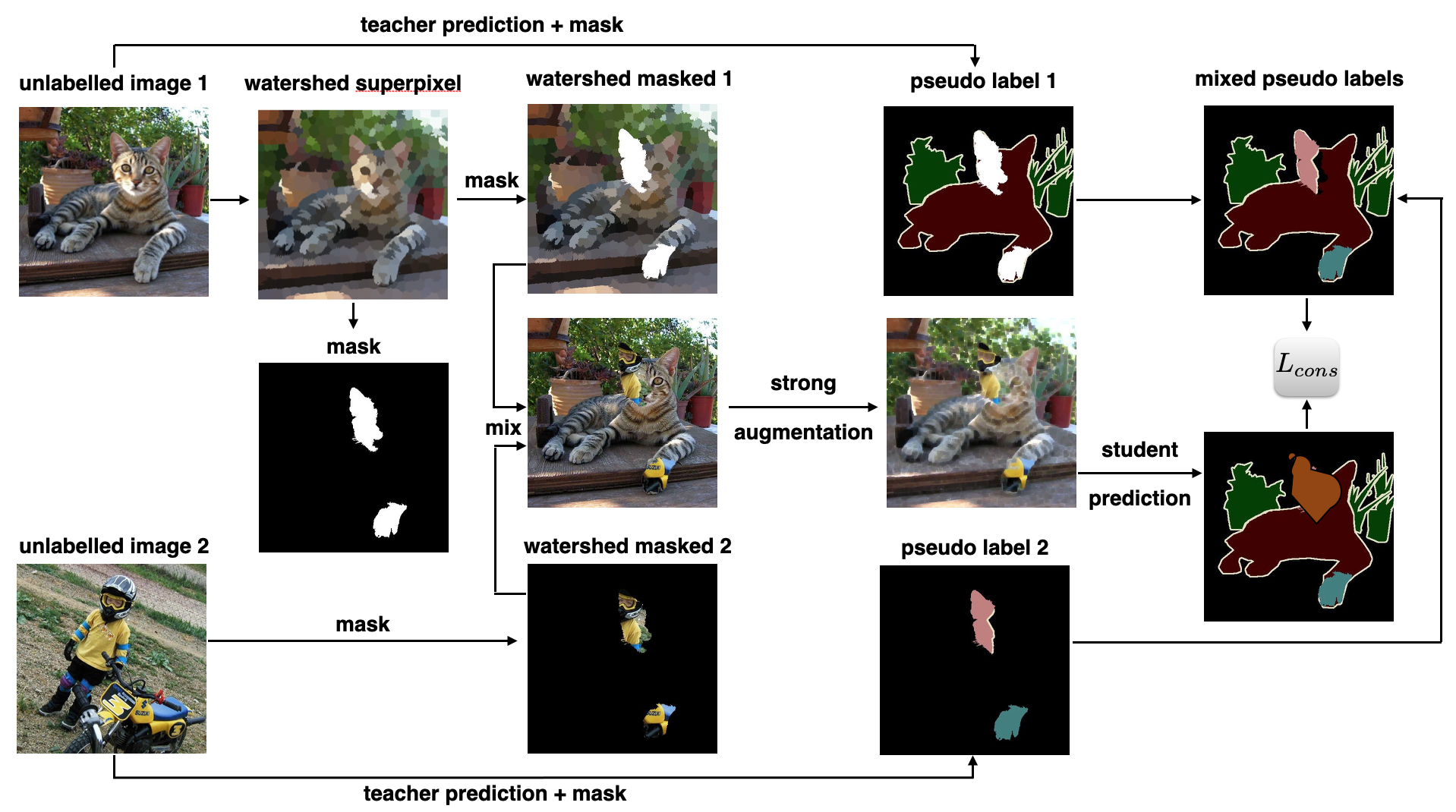
Figure 1: Consistency training with a student-teacher framework using unlabeled images (Task 2). To mix two unlabeled images, superpixels are randomly sampled to create a mixing mask. This mask is used to merge the two images and their pseudo-label outputs from the teacher network. A cross-entropy loss is applied to the student network to encourage consistency between the mixed pseudo-labels and the student network labels.

In this paper, we propose a novel superpixel-mix method to generate new training data and leverage the results of this data augmentation technique in an existing teacher-student framework [Tarvainen and Valpola(2017)]. The combination of our mixing technique and the teacher-student framework forms an optimization component that serves as a consistency constraint in our DCNN training system for semantic segmentation. We conduct experiments for evaluating our trained DCNNs on both types of uncertainties: epistemic and aleatoric. At the end, we also assess our proposed approach in semi-supervised learning.

In general, our training process for all of our experiments comprises two steps that are optimized simultaneously: (1) supervised learning where we train the DCNNs using images with ground-truth labels, and (2) using teacher-student optimization with superpixel-mix data augmentation on images as a consistency constraint that does not use ground-truth labels. In the uncertainty experiments such as OOD in § 4.2, DCNNs’ bias studying in § 4.3, and aleatoric uncertainty in § 4.4, we use datasets that contain ground-truth labels for all images. We first train the DCNNs in fully supervised learning fashion as in step 1. We then remove all those labels and use only the images to optimize for the consistency constraint as in step 2. In the semi-supervised learning experiment in § 4.5, we use the training dataset that consists of two parts: labelled images and unlabelled images. We train the DCNN using the labelled data for step 1 and the unlabelled data for step 2.

Step 1 - supervised learning with labelled images: We use a standard pixel-wise cross-entropy loss denoted by $\mathcal{L}_{\text{sup}}$ and apply it to all the labelled images. In addition, we use a weak data augmentation (WDA) that consists of horizontal flipping and/or random cropping.

Step 2 - consistency constraint with unlabelled images: We apply two transformations on an unlabelled image: one is WDA and the other is a strong data augmentation (SDA). Consistency training encourages predictions of the DCNNs to be consistent in the results of the two transformations. For SDA, we merge WDA and a superpixel mixing technique (see § 3.3). The consistency loss for optimizing this constraint is denoted as $\mathcal{L}_{\text{cons}}$.

For every experiment, we optimize the loss in the overall framework as the joint loss $\mathcal{L}=\mathcal{L}_{\text{sup}}+\lambda\cdot\mathcal{L}_{\text{cons}}$, where $\lambda$ is a weighting hyper-parameter and is set to 1.

3.2 Teacher-Student Framework

To learn from unlabeled images, we follow the teacher-student framework established in [Tarvainen and Valpola(2017)], where the teacher network produces pseudo-labels learned from the labeled data and the student network is encouraged to be consistent with the teacher. Consistency is encouraged via cross-entropy loss between the two outputs. In our case, we encourage consistency between the mixed output labels of a teacher network corresponding to the two unlabelled inputs and the output label of a student network predicted from the input that resulted by mixing the two unlabelled images. We explain this approach in details in the following paragraph.

Let $g_{\phi}$ represent the teacher network with weights $\phi$ and $f_{\theta}$ be the student network with weights $\theta$. For two unlabeled images $x^{1}_{u}$ and $x^{2}_{u}$, we can use the teacher network to generate pseudo-labels $y^{1}_{u}$ and $y^{2}_{u}$: $y^{1}_{u}=g_{\phi}(x^{1}_{u})$ and $y^{2}_{u}=g_{\phi}(x^{2}_{u})$. Assume now we are given some mixing function mix with a mixing parameter $m$. Without any assumption on the mixing itself, we denote a mixed output label $y_{m}$, where $y_{m}=\texttt{mix}(y^{1}_{u},y^{2}_{u},m)$. For the same mixing parameter $m$, we can also mix the inputs $x^{1}_{u}$ and $x^{2}_{u}$, i.e. $x_{m}=\texttt{mix}(x^{1}_{u},x^{2}_{u},m)$. Applying $x_{m}$ to the student network, we expect $f_{\theta}(x_{m})$ to be the same as the mixed output $y_{m}$. This is enforced by minimizing the consistency loss $\mathcal{L}_{\text{cons}}=\text{CE}\left(y_{m},f_{\theta}\left(\texttt{mix}(x^{1}_{u},x^{2}_{u},m)\right)\right)$, where CE is the pixel-wise cross-entropy and $y_{m}$ is the mixed pseudo-labels from the teacher.

During training, both the teacher and student networks evolve together. Similarly to [Tarvainen and Valpola(2017)], we update the teacher network weights $\phi$ after each iteration with an Exponential Moving Average (EMA), i.e. $\phi=\alpha\phi+(1-\alpha)\theta$ where $\alpha=0.99$ is a momentum-like parameter.

3.3 Superpixel-mix for semantic segmentation

To mix two unlabeled images, we use masks generated by sampling superpixels. Superpixels are local clusters of visually similar pixels. Therefore, a group of pixels belonging to the same superpixel are likely to be in the same object or the same part of the object. There are several superpixel variants, including SEEDS [Van den Bergh et al.(2012)Van den Bergh, Boix, Roig, de Capitani, and Van Gool], SLIC [Achanta et al.(2012)Achanta, Shaji, Smith, Lucchi, Fua, Süsstrunk, et al.] or Watershed superpixels [Machairas et al.(2014)Machairas, Decencière, and Walter]. We opt to use Watershed superpixels as their boundaries retain more salient object edges [Machairas et al.(2015)Machairas, Faessel, Cárdenas-Peña, Chabardes, Walter, and Decencière]. We refer the reader to the Supplementary Material for details on how we use the watershed transformation to produce superpixels.

Given an unlabeled image $x^{1}_{u}$, we apply the watershed superpixel algorithm, which results in a set of $n$ superpixels $\mathcal{S}=\{S_{1},S_{2},...,S_{n}\}$. A mixing mask $m$ (which is a binary mask) is created from a sampled subset of superpixels $S$: $m=\cup_{j\in\sigma(k,n)}S_{j}$ where $\sigma(k,n)$ is a subset of size $k$ of the $n$ indices, and $k$ is the number of superpixels we want to keep.

The mixing mask $m$ defines the pixels in $x^{1}_{u}$ which will be replaced by pixels from the unlabeled image $x^{2}_{u}$ to form the mixed input $x_{m}$, i.e. $x_{m}=\texttt{mix}(x^{1}_{u},x^{2}_{u},m)=(1-m)\odot x^{1}_{u}+m\odot x^{2}_{u}$, where $\odot$ is a pixel-wise multiplication. Superpixels are uniformly sampled given a fixed proportion of selected superpixels. Contrary to existing regularization techniques such as Cutout [DeVries and Taylor(2017)] or Cutmix [French et al.(2020)French, Laine, Aila, Mackiewicz, and Finlayson], our superpixel mixing strategy enforces each set of selected pixels in the unlabeled image $x^{1}_{u}$ to belong to the same object. However, the algorithm is allowed to select a set of superpixel clusters from different objects as illustrated in Figure 1.

We use 200 superpixels per image for all the evaluated datasets. Studies on the number and proportions of superpixels used in mixing are shown in Section 4.6 and the Supplement.

3.4 From empirical risk to teacher-student mixup

In this section, we show that the training loss of the teacher-student framework in combination with superpixel-mix data augmentation is bounded by the accuracy of the teacher network and the quality of the data augmentation. Let $\mathcal{D}=\{(x_{i},y_{i})\}_{i}\sim\mathcal{P}$ be the labelled dataset which follows the joint distribution $\mathcal{P}$ and $l$ be a loss between the target $y$ and the prediction $f_{\theta}(x)$ of the DCNN $f_{\theta}$. Typically, in deep learning, the objective is to learn $\theta$ that minimizes the expected risk defined by: $\mathbf{R}_{\mathcal{P}}(f_{\theta})=\int l(f_{\theta}(x),y)d\mathcal{P}(x,y)$. As we do not have access to the distribution $\mathcal{P}$, we optimize the loss function that is formed by the empirical risk on $\mathcal{D}$:

$$\hat{\mathbf{R}}_{\mathcal{P}_{\delta}}(f_{\theta})=\frac{1}{n}\sum_{i=1}^{n}l(f_{\theta}(x_{i}),y_{i})=\int l(f_{\theta}(x),y)d\mathcal{P}_{\delta}(x,y),$$ (1)

where the summation is converted back to the integral based on $\mathcal{P}_{\delta}(x,y)=\frac{1}{n}\sum_{i=1}\delta(x=x_{i},y=y_{i})$, as shown by [Zhang et al.(2017)Zhang, Cisse, Dauphin, and Lopez-Paz].

Therefore, we optimize the parameters of the DCNN using the empirical risk. However, the representation of the discretized data is likely to be sparse, Zhang et al [Zhang et al.(2017)Zhang, Cisse, Dauphin, and Lopez-Paz] proposed to work with $\mathcal{D}_{\text{mix}}=\{(x_{m,i},y_{m,i})\}_{i}\sim\mathcal{P}^{\text{mix}}_{X,Y}$ where $x_{m,i}$, and $y_{m,i}$ are the data of $\mathcal{D}$ where a mixing procedure has been applied. The hypothesis in [Zhang et al.(2017)Zhang, Cisse, Dauphin, and Lopez-Paz] is that the mixing procedure helps to better approximate the dataset distribution. Let $\mathcal{P}^{\text{mix}}_{\delta}$ denote the discrete distribution of this augmented dataset. The risk to fit the teacher prediction on $\mathcal{P}^{\text{mix}}_{\delta}$ can then be defined as: $\hat{\mathbf{R}}_{\mathcal{P}^{\text{mix}}_{\delta}}(f_{\theta},g_{\phi})=\int l(f_{\theta}(x),g_{\phi}(x))d\mathcal{P}^{\text{mix}}_{\delta}(x,y).$ Therefore, our training loss for the overall framework is defined in detail as the following: $\mathcal{L}(\theta)=\hat{\mathbf{R}}_{\mathcal{P}_{\delta}}(f_{\theta})+\hat{\mathbf{R}}_{\mathcal{P}^{\text{mix}}_{\delta}}(f_{\theta},g_{\phi}).$ As the loss $l$ is a norm that satisfies the triangle equality, we can prove that the training loss $\mathcal{L}(\theta)$ is bounded by the following:

$$\mathcal{L}(\theta)\leq 2\mathbf{R}_{\mathcal{P}}(f_{\theta})+M(\|\mathcal{P}^{\text{mix}}_{\delta}-\mathcal{P}\|_{1}+\|\mathcal{P}_{\delta}-\mathcal{P}\|_{1})+\hat{\mathbf{R}}_{\mathcal{P}^{\text{mix}}_{\delta}}(g_{\phi}),$$ (2)

where the four terms are linked to the true error, approximation error, mixing distribution error and teacher error, respectively. This implies that the quality of the DCNN is bounded by the accuracy of the teacher. It is also bounded by how much the mixing strategy can sample the true distribution of the dataset. Finally, the distribution of the training data with respect to the true data distribution also plays an important role. This finding can be applied to all teacher-student frameworks, such as those used in SSL, self supervised training, and domain adaptation. The detailed proof and analysis is given in the Supplementary Material.

$\|\mathcal{P}^{\text{mix}}_{\delta}-\mathcal{P}\|_{1}$ and $\|\mathcal{P}_{\delta}-\mathcal{P}\|_{1}$ reflect the capacity of the two distributions $\mathcal{P}_{\delta}$ and $\mathcal{P}^{\text{mix}}_{\delta}$ to approximate the true dataset distribution. This bound allows us to control the variation of the risk. To reduce the risk, we can increase the number of training data or improve the quality of the data augmentation and so reduce $\|\mathcal{P}^{\text{mix}}_{\delta}-\mathcal{P}\|_{1}$. This motivates our research on data augmentation strategies to approximate the true distribution in a data-efficient way. We can also improve the quality of the teacher using EMA training that stabilizes the training loss.

3.5 Uncertainty and Deep Learning

Consider a joint distribution $\mathcal{P}$ over input $x$ and labels $y$ over a set of labels $\mathcal{Y}$. When a DCNN performs inference, it predicts $f_{\theta}=\mathcal{P}(y|x,\theta)$, where $\theta$ is optimized to minimize the loss over the training set $\mathcal{D}$. This likelihood typically suffers from two kinds of uncertainty [Hora(1996), Kendall and Gal(2017)]. First is aleatoric uncertainty, linked to the unpredictability of the data acquisition process. During inference, instead of working with $x$, we may have access to $x+n$, where $n$ represents noise on the input data. Second is epistemic uncertainty, linked to the lack of knowledge of the model, i.e., the weights $\theta$ of the network. In addition, the epistemic uncertainty can be subdivided into two sub-types: one linked to the OOD  [Malinin and Gales(2018)] and the other one linked to networks’ bias. Epistemic uncertainty models the uncertainty associated with limited sizes of training datasets. Most works focus only on the ability to detect OOD. In this paper, we conduct experiments for all types of uncertainties: aleatoric (i.e., testing models on noisy data) and two sub-types of epistemic (i.e., OOD detection and models’ bias).

4 Experiments

We conduct experiments on five datasets. First, we study network robustness to epistemic uncertainty experiments on StreetHazards [Hendrycks et al.(2019)Hendrycks, Basart, Mazeika, Mostajabi, Steinhardt, and Song]. The test set contains some object classes that are not available in the training set. The goal is to detect these out-of-distribution (OOD) classes. We also evaluate the performance of the DCNNs on an contextually unbiased dataset. Furthermore, we investigate the networks’ robustness for the aleatoric uncertainty. To this end, we train a DCNN on Cityscapes  [Cordts et al.(2016)Cordts, Omran, Ramos, Rehfeld, Enzweiler, Benenson, Franke, Roth, and Schiele] and evaluate the performances on Rainy [Hu et al.(2019)Hu, Fu, Zhu, and Heng] and Foggy Cityscapes [Sakaridis et al.(2018)Sakaridis, Dai, and Van Gool]. Finally, we evaluate on the semi-supervised learning task on Cityscapes [Cordts et al.(2016)Cordts, Omran, Ramos, Rehfeld, Enzweiler, Benenson, Franke, Roth, and Schiele] and Pascal  [Everingham et al.(2012)Everingham, Van Gool, Williams, Winn, and Zisserman]. We implement the experiments using PyTorch (see Supplementary Material).

4.1 Evaluation criteria

The first criterion we use is the mIoU [Jaccard(1912)], reflecting the predictive performance of segmentation models. Second, similarly to [Lakshminarayanan et al.(2017)Lakshminarayanan, Pritzel, and Blundell] we use the negative log-likelihood (NLL), a proper scoring rule [Gneiting and Raftery(2007)], which depends on the aleatoric uncertainty and can assess the degree of overfitting [Guo et al.(2017)Guo, Pleiss, Sun, and Weinberger].. In addition, we use the expected calibration error (ECE)  [Guo et al.(2017)Guo, Pleiss, Sun, and Weinberger] that measures how the confidence score predicted by a DCNN is related to its accuracy. Finally, we use the AUPR , AUC, and the FPR-95-TPR defined in [Hendrycks and Gimpel(2017)] that evaluate the quality of a DCNN to detected OOD data. With multiple metrics, we can get a clearer picture on the performance of the DCNNs with regards to accuracy, calibration error, failure rate, OOD detection. Even though it is difficult to achieve top performance on all metrics, we argue that it is more pragmatic and convincing to evaluate on multiple metrics [Ovadia et al.(2019)Ovadia, Fertig, Ren, Nado, Sculley, Nowozin, Dillon, Lakshminarayanan, and Snoek, Fort et al.(2019)Fort, Hu, and Lakshminarayanan] than optimizing for a single metric, potentially at the expense of many others. For example, a DCNN with a low accuracy and a low confidence score is well-calibrated. Therefore, evaluating a DCNN on a single metric such as ECE or mIoU alone is not enough. We aim to have a good compromise between accuracy and calibration.

4.2 Epistemic uncertainty: Out-Of-Distribution (OOD) Detection

One cause of the epistemic uncertainty in deep learning is the limited training data that does not cover all possible object classes. The evaluation of this type of epistemic uncertainty is often linked to OOD detection. Therefore, this experiment is designed to evaluate the epistemic uncertainty using StreetHazards [Hendrycks et al.(2019)Hendrycks, Basart, Mazeika, Mostajabi, Steinhardt, and Song]. StreetHazards is a large-scale dataset that consists of different sets of synthetic images of street scenes. This dataset is composed of $5,125$ images for training and $1,500$ test images. The training dataset contains pixel-wise annotations for $13$ classes. The test dataset comprises $13$ training classes and $250$ OOD classes, unseen in the training set, making it possible to test the robustness of the algorithm when facing a diversity of possible scenarios. For this experiment, we use DeepLabv3+ [Chen et al.(2018)Chen, Zhu, Papandreou, Schroff, and Adam] with the experimental protocol from [Hendrycks et al.(2019)Hendrycks, Basart, Mazeika, Mostajabi, Steinhardt, and Song]. We use ResNet50 encoder [He et al.(2016)He, Zhang, Ren, and Sun]. For this experiment, we compare our algorithm to Deep Ensembles [Lakshminarayanan et al.(2017)Lakshminarayanan, Pritzel, and Blundell], BatchEnsemble [Wen et al.(2020)Wen, Tran, and Ba], LP-BNN [Franchi et al.(2020b)Franchi, Bursuc, Aldea, Dubuisson, and Bloch], TRADI [Franchi et al.(2020a)Franchi, Bursuc, Aldea, Dubuisson, and Bloch] , MIMO [Havasi et al.(2020)Havasi, Jenatton, Fort, Liu, Snoek, Lakshminarayanan, Dai, and Tran] achieving state-of-the-art results on epistemic uncertainty. We also compare our model with MCP which is the baseline DCNN where we consider the maximum probability class as a confidence score, and with Cutmix [French et al.(2020)French, Laine, Aila, Mackiewicz, and Finlayson] strategy. The results in Table 1 show that our method is the only one to have the best results in three out of five measures. Running up, Deep Ensemble and LP-BNN achieve best results on one measure only. Moreover, our method achieves the best results faster than Deep Ensemble and LP-BNN, we only need one inference pass compared to 4 inference passes for the others.

Dataset	OOD method	mIoU $\uparrow$	AUC $\uparrow$	AUPR $\uparrow$	FPR-95-TPR $\downarrow$	ECE $\downarrow$	# Forward passes $\downarrow$
StreetHazards DeepLabv3+ ResNet50	Baseline (MCP) [Hendrycks and Gimpel(2017)]	53.90%	0.8660	0.0691	0.3574	0.0652	1
	TRADI [Franchi et al.(2020a)Franchi, Bursuc, Aldea, Dubuisson, and Bloch]	52.46%	0.8739	0.0693	0.3826	0.0633	4
	Cutmix  [French et al.(2020)French, Laine, Aila, Mackiewicz, and Finlayson]	56.06%	0.8764	0.0770	0.3236	0.0592	1
	MIMO [Havasi et al.(2020)Havasi, Jenatton, Fort, Liu, Snoek, Lakshminarayanan, Dai, and Tran]	55.44%	0.8738	0.0690	0.3266	0.0557	4
	BatchEnsemble [Wen et al.(2020)Wen, Tran, and Ba]	56.16%	0.8817	0.0759	0.3285	0.0609	4
	LP-BNN [Franchi et al.(2020b)Franchi, Bursuc, Aldea, Dubuisson, and Bloch]	54.50%	0.8833	0.0718	0.3261	0.0520	4
	Deep Ensembles [Lakshminarayanan et al.(2017)Lakshminarayanan, Pritzel, and Blundell]	55.59%	0.8794	0.0832	0.3029	0.0533	4
	Superpixel-mix (ours)	56.39%	0.8891	0.0778	0.2962	0.0567	1

Table 1: Comparative results on the OOD task for semantic segmentation. Results are averaged over three seeds.

4.3 Epistemic uncertainty : Unbiased experiment

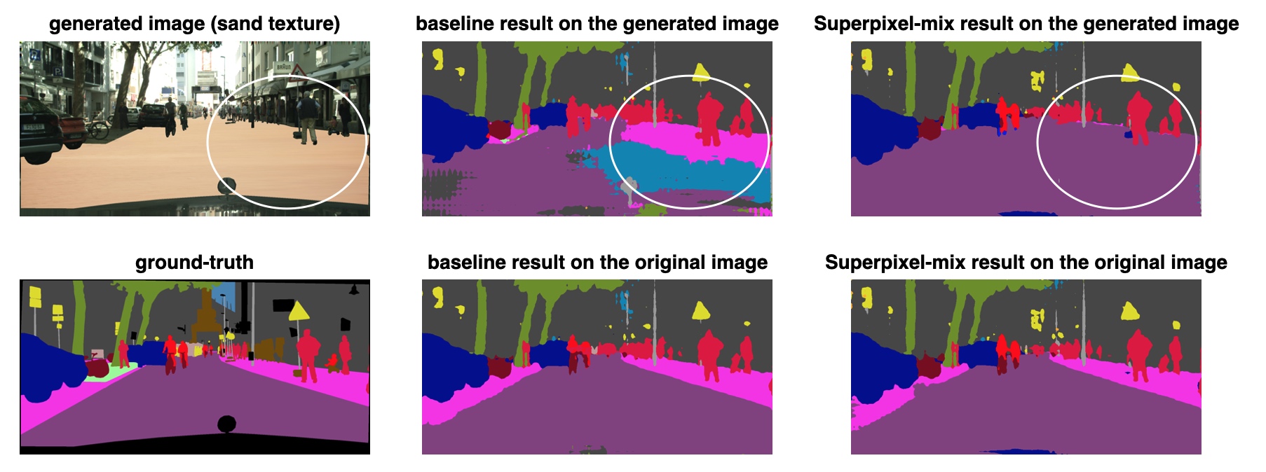
Figure 2: A qualitative example of the network bias study. When the road and pavements are replaced with sand texture, the baseline supervised network makes wrong segmentations. There is still pavement segmentation due to the association with people. Superpixel-mix produces better results without the wrong pavement segmentation, also provides a clean segmentation for the sand texture.

The second aspect of epistemic uncertainty is related to network biased caused limited samples and diversity of scenarios, e.g., certain objects always co-occur in the training data. Here, we evaluate the epistemic uncertainty under the lens of model bias. In urban datasets such as Cityscapes, road and car pixels appear most of the time together, raising the question of co-occurrence dependency between objects. If two objects are dependent, then the network will likely fail when the car object is encountered in different context other than roads. Shetty et al [Shetty et al.(2019)Shetty, Schiele, and Fritz] study object dependency and suggest using GANs to remove one object by in-painting and training the network for the new contexts. Their results show that a network that is less biased towards the co-occurrence dependency yields better accuracy for segmentation.

To measure the bias of our superpixel-mix method, we create a new dataset dubbed Out-of-Context Cityscapes (OC-Cityscapes), by replacing roads in the validation data of Cityscapes with various textures such as water, sand, grass, etc. Example images are shown in the Supplementary Material. Studies in [Geirhos et al.(2019)Geirhos, Rubisch, Michaelis, Bethge, Wichmann, and Brendel] show that DCNNs are biased towards texture. By replacing different textures for roads, we test the trained networks on these new context images and evaluate the bias level for each network.

In Table 2, we show the performances of the fully supervised network (baseline) and our network trained using the superpixel-mix method for the Cityscapes validation set and our generated dataset. The results are mIoU, ECE, and NLL scores averaged over 3 runs for classes that are not road. On our experimental dataset, the baseline’s performance drops by 21.97% while Superpixel-mix drops by 19.83% for the mIoU metric. The results also show that Superpixel-mix produces a less biased model for co-occurring objects with the best scores on mIoU and NLL measures. Superpixel-mix changes the image context while preserving object shapes, effectively regularizing the model to address shortcut learning, i.e., overfitting on the co-occurrence of objects and their typical contexts. For a visual example, see Figure 2.

Evaluation data	Cityscapes	OC-Cityscapes	Cityscapes	OC-Cityscapes	Cityscapes	OC-Cityscapes
	mIoU	mIoU	NLL	NLL	ECE	ECE
Baseline (MCP) [Hendrycks and Gimpel(2017)]	76.51%	54.54%	-0.9456	-0.7565	0.1303	0.2162
Cutmix  [French et al.(2020)French, Laine, Aila, Mackiewicz, and Finlayson]	78.37%	54.78%	-0.955	-0.7435	0.1365	0.2587
MIMO [Havasi et al.(2020)Havasi, Jenatton, Fort, Liu, Snoek, Lakshminarayanan, Dai, and Tran]	77.13%	55.87%	-0.9516	-0.7431	0.1398	0.2359
Deep Ensembles [Lakshminarayanan et al.(2017)Lakshminarayanan, Pritzel, and Blundell]	77.48%	57.09%	-0.9469	-0.7613	0.1274	0.1968
Superpixel-mix (ours)	78.99%	59.16%	-0.9563	-0.7768	0.1348	0.2244

Table 2: Comparative results for network biases on OC-Cityscapes. The results are segmentation mIoU, NLL and ECE, for classes that are not road. The baseline is the result from supervised training.

4.4 Aleatoric uncertainty experiments

Aleatoric uncertainty is associated with unpredictability of the data acquisition process that causes various noises in the data. In the following experiments we evaluate the aleatoric uncertainty of DCNNs trained on normal images (e.g., normal weather images) when facing test images with various types of noise (e.g., rainy or foggy environments). In semantic segmentation, the DCNN must be robust to aleatoric uncertainty. To check that, we use the rainy [Hu et al.(2019)Hu, Fu, Zhu, and Heng] and foggy Cityscapes [Sakaridis et al.(2018)Sakaridis, Dai, and Van Gool] datasets, which are built by adding rain of fog to the Cityscapes validation images. The goal is to evaluate the performance of DNNs to resist these perturbations. We further generate an additional Cityscapes variant with images modified with different perturbations and intensities to mimic a distribution shift [Hendrycks and Dietterich(2019)]. We apply the following perturbations: Gaussian noise, shot noise, impulse noise, defocus blur, frosted, glass blur, motion blur, zoom blur, snow, frost, fog, brightness, contrast, elastic, pixelate, JPEG. For more information, please refer to [Hendrycks and Dietterich(2019)]. We call this dataset Cityscapes-C.

To measure the robustness under aleatoric uncertainty, we compute ECE, mIoU and NLL scores averaged over 3 runs. Table 3 shows results close to the state of the art. DE reaches good results, yet this approach needs to train several DCNNs, so it is more time-consuming for training and inference. In the Supplementary Material, we report mIoU scores of different approaches for the different levels of noise. Overall, our experiments indicate that Superpixel-mix tends to be robust to high level of noise.

Evaluation data	Cityscapes			Rainy Cityscapes			Foggy Cityscapes			Cityscapes-C
	mIoU $\uparrow$	ECE $\downarrow$	NLL $\downarrow$	mIoU $\uparrow$	ECE $\downarrow$	NLL $\downarrow$	mIoU $\uparrow$	ECE $\downarrow$	NLL $\downarrow$	mIoU $\uparrow$	ECE $\downarrow$	NLL $\downarrow$
Baseline (MCP) [Hendrycks and Gimpel(2017)]	76.51%	0.1303	-0.9456	58.98%	0.1395	-0.8123	69.89%	0.1493	-0.9001	40.85%	0.2242	-0.7389
Cutmix  [French et al.(2020)French, Laine, Aila, Mackiewicz, and Finlayson]	78.37%	0.1365	-0.9550	61.86%	0.1559	-0.8200	73.57%	0.1484	-0.9289	39.16%	0.3064	-0.6865
MIMO [Havasi et al.(2020)Havasi, Jenatton, Fort, Liu, Snoek, Lakshminarayanan, Dai, and Tran]	77.13%	0.1398	-0.9516	59.27%	0.1436	-0.8135	70.24%	0.1425	-0.9014	40.73%	0.2350	-0.7313
BatchEnsemble [Wen et al.(2020)Wen, Tran, and Ba]	77.99%	0.1129	-0.9472	60.29%	0.1436	-0.7820	72.19%	0.1425	-0.9132	40.93%	0.2270	-0.7082
LP-BNN [Franchi et al.(2020b)Franchi, Bursuc, Aldea, Dubuisson, and Bloch]	77.39%	0.1105	-0.9464	60.71%	0.1338	-0.7891	72.39%	0.1358	-0.9131	43.47%	0.2085	-0.7282
Deep Ensembles [Lakshminarayanan et al.(2017)Lakshminarayanan, Pritzel, and Blundell]	77.48%	0.1274	-0.9469	59.52%	0.1078	-0.8205	71.43%	0.1407	-0.9070	43.40%	0.1912	-0.7509
Superpixel-mix (ours)	78.99%	0.1348	-0.9563	61.87%	0.1583	-0.8207	74.39%	0.1411	-0.9266	42.58%	0.2338	-0.7513

Table 3: Aleatoric uncertainty study on Cityscapes-C, Foggy Cityscapes [Hu et al.(2019)Hu, Fu, Zhu, and Heng] and Rainy Cityscapes [Sakaridis et al.(2018)Sakaridis, Dai, and Van Gool].

We note that our method does not achieve the top ECE scores across the various perturbations and weather conditions in these experiments. However, none of the considered strong baselines based on ensembles outperforms the others consistently either due to the difficulty and diversity of the considered test sets. Superpixel-mix achieves competitive ECE scores and is a top performer on mIoU and NLL.

4.5 Semi-Supervised Learning experiments

To evaluate the robustness of our method to missing annotation, we tested our approach on a semi-supervised learning task on two datasets: Cityscapes [Cordts et al.(2016)Cordts, Omran, Ramos, Rehfeld, Enzweiler, Benenson, Franke, Roth, and Schiele] and Pascal VOC 2012 [Everingham et al.(2012)Everingham, Van Gool, Williams, Winn, and Zisserman]. We follow the common practice for this task from prior works [Hung et al.(2018)Hung, Tsai, Liou, Lin, and Yang, French et al.(2020)French, Laine, Aila, Mackiewicz, and Finlayson] and use DeepLab-V2 [Chen et al.(2017)Chen, Papandreou, Kokkinos, Murphy, and Yuille] model with ResNet101 [He et al.(2016)He, Zhang, Ren, and Sun] encoder pre-trained on ImageNet [Deng et al.(2009)Deng, Dong, Socher, Li, Kai Li, and Li Fei-Fei] and MS-COCO [Lin et al.(2014)Lin, Maire, Belongie, Hays, Perona, Ramanan, Dollár, and Zitnick]. The weights of both the teacher and student models are initialized the same manner. We evaluate our method and compare with existing methods using three sets of labeled data: 1/30 (100 images), 1/8 (372 images) and 1/4 (744 images). Our results are reported as average mIoU of 12 runs (4 times on each of 3 official splits) as well as the standard deviation. The results are shown in Table 4. We present results on Pascal dataset in the Supplementary Material.

Labeled samples	1/30 (100)	1/8 (372)	1/4 (744)
Adversarial [Hung et al.(2018)Hung, Tsai, Liou, Lin, and Yang]	-	58.80%	62.30%
s4GAN [Mittal et al.(2019)Mittal, Tatarchenko, and Brox]	-	59.30%	61.90%
Cutout [DeVries and Taylor(2017)]	47.21% $\pm$ 1.74	57.72% $\pm$ 0.83	61.96% $\pm$ 0.99
Cutmix [French et al.(2020)French, Laine, Aila, Mackiewicz, and Finlayson]	51.20% $\pm$ 2.29	60.34% $\pm$ 1.24	63.87% $\pm$ 0.71
Classmix [Olsson et al.(2020)Olsson, Tranheden, Pinto, and Svensson]	54.07% $\pm$ 1.61	61.35% $\pm$ 0.62	63.63% $\pm$ 0.33
Classmix [Olsson et al.(2020)Olsson, Tranheden, Pinto, and Svensson]	54.07% $\pm$ 1.61	61.35% $\pm$ 0.62	63.63% $\pm$ 0.33
Baseline(*)	43.84% $\pm$ 0.71	54.84% $\pm$ 1.14	60.08% $\pm$ 0.62
Superpixel-mix (ours)	54.11% $\pm$ 2.88 ($\uparrow$ 7.27%)	63.44%$\pm$ 0.88 ($\uparrow$ 8.60%)	65.82%$\pm$ 1.78 ($\uparrow$ 5.74%)

Table 4: Evaluation in the semi-supervised learning regime on Cityscapes. We report mIoU scores as $mean\pm std.dev$ computed over 12 runs. The $(\uparrow)$ shows the improvement of our methods over the baselines. (*) The baselines are from [Olsson et al.(2020)Olsson, Tranheden, Pinto, and Svensson] as we use a similar base procedure.

4.6 Ablations and analysis

We perform various ablations to understand the influence of different hyper-parameters and choices in our algorithm. First, we vary the number of superpixels extracted per image from 20 to 1,000. The results (in Table 5, Supplement) show that our method achieves the highest mIoU on Cityscapes when the number of superpixels per image is from 100 to 200. Secondly, we study the proportion of chosen superpixels for mixing over the total number of superpixels per image. The proportion ranges from 0.1 to 0.9. We find that the results vary little across all the proportion values (Table 6, Supplement). The best mIoU is obtained at the proportion value of 0.6. Finally, we study the influence of different superpixel techniques to generate mixing masks: Watershed [Machairas et al.(2014)Machairas, Decencière, and Walter], SLIC [Achanta et al.(2012)Achanta, Shaji, Smith, Lucchi, Fua, Süsstrunk, et al.], and Felzenszwalb [Felzenswalb and Huttenlocher(2004)]. The results in Table 5 show that on Cityscapes segmentation the performance of Superpixel-mix is relatively stable across superpixel methods, with Watershed yielding the best mIoU score.

superpixels algorithm	Watershed  [Machairas et al.(2014)Machairas, Decencière, and Walter]	SLIC [Achanta et al.(2012)Achanta, Shaji, Smith, Lucchi, Fua, Süsstrunk, et al.]	Felzenszwalb [Felzenswalb and Huttenlocher(2004)]
mIoU	78.99 %	78.89%	77.99%

Table 5: Ablation study results over influence of different superpixel techniques. We report mIoU scores for semantic segmentation on Cityscapes.

5 Conclusions

Superpixel-mix data augmentation is a promising new training technique for semantic segmentation. This strategy for creating diverse data, combined with a teacher-student framework, leads to better accuracy and to more robust DCNNs. We are the first, to the best of our knowledge, to successfully apply the watershed algorithm in data augmentation. What sets our data augmentation technique apart from existing methods is the ability to preserve the global structure of images and the shapes of objects while creating image perturbations. We conduct various experiments with different types of uncertainty. The results show that our strategy achieves state-of-the-art robustness scores for epistemic uncertainty. For aleatoric uncertainty, our approach produces state-of-the-art results in Foggy Cityscapes and Rainy Cityscapes. In addition, our method needs just one forward pass.

Previous research in machine learning has established that creating more training data using data augmentation may improve the accuracy of the trained DCNNs substantially. Our work not only confirms that, but also provides evidence that some data augmentation methods, such as our Superpixel-mix, help to improve the robustness of DCNNs by reducing both epistemic and aleatoric uncertainty.

Robust Semantic Segmentation with Superpixel-Mix (Supplementary material)

6 Watershed tranform for Superpixel-mix

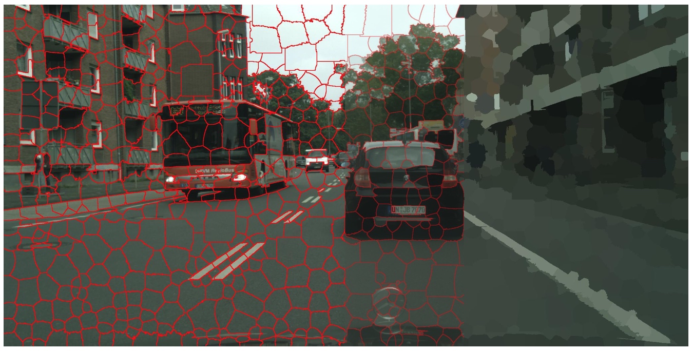
Figure 3: An example of superpixels on an image from Cityscapes dataset.

To mix two unlabeled images, we use masks generated from randomly sampled superpixels. Superpixels are local clusters of visually similar pixels, typically delimited by pronounced edges (as illustrated in Figure 3). Therefore, a group of pixels belonging to the same superpixel are likely to correspond to the same object or a part of an object. There are various methods for computing superpixels, including SEEDS [Van den Bergh et al.(2012)Van den Bergh, Boix, Roig, de Capitani, and Van Gool], SLIC [Achanta et al.(2012)Achanta, Shaji, Smith, Lucchi, Fua, Süsstrunk, et al.] or Watershed [Machairas et al.(2014)Machairas, Decencière, and Walter]. We opt to use Watershed superpixels as their boundaries retain more salient object edges [Machairas et al.(2015)Machairas, Faessel, Cárdenas-Peña, Chabardes, Walter, and Decencière].

Watershed transformation and all its variants [Beucher(1994), Beucher and Meyer(1993), Beucher(1979)] are powerful techniques for image segmentation. Watershed processes image gradients and outputs corresponding clusters for each pixel. Since the watershed input is a gradient, we convert the input image from RGB to Lab in order to compute the gradient maps. Then, on each channel, we evaluate a morphological gradient and we average the three results. Similarly to [Machairas et al.(2014)Machairas, Decencière, and Walter], instead of considering all the clusters of the watershed, we build a regular grid of points and consider these points as markers for the watershed transform. This strategy allows us to control the number of superpixels to reduce computational cost.

7 From empirical risk to teacher student mixup

In this section, we show that the training loss of the teacher-student framework in combination with superpixel-mix data augmentation is bounded by the accuracy of the teacher network and the quality of the data augmentation. This result is essential since it is the first bound for a teacher-student framework with consistency training. Different and effective variants of teacher-students approaches with consistency training have emerged in recent literature, in particular in semi-supervised learning [Berthelot et al.(2019b)Berthelot, Carlini, Goodfellow, Papernot, Oliver, and Raffel, Berthelot et al.(2019a)Berthelot, Carlini, Cubuk, Kurakin, Sohn, Zhang, and Raffel, Sohn et al.(2020)Sohn, Berthelot, Li, Zhang, Carlini, Cubuk, Kurakin, Zhang, and Raffel] and self-supervised learning [Grill et al.(2020)Grill, Strub, Altché, Tallec, Richemond, Buchatskaya, Doersch, Pires, Guo, Azar, et al., Gidaris et al.(2020)Gidaris, Bursuc, Komodakis, Pérez, and Cord, Chen and He(2021)]. All these approaches rely heavily on well-crafted agressive data augmentation strategies. This result could be useful in this context as we proove how the quality of the teacher and the quality of the data augmentation influence the accuracy of the student.

Let $\mathcal{D}=\{(x_{i},y_{i})\}\sim\mathcal{P}$ be the labelled dataset which follows the joint distribution $\mathcal{P}$ and $l$ be a loss between the target $y$ and the prediction $f_{\theta}(x)$ of the DCNN $f_{\theta}$. Typically, in deep learning, the objective is to learn $\theta$ that minimizes the expected risk defined by: $\mathbf{R}_{\mathcal{P}}(f_{\theta})=\int l(f_{\theta}(x),y)d\mathcal{P}(x,y)$. As we do not have access to the distribution $\mathcal{P}$, we optimize the loss function that is formed by the empirical risk on $\mathcal{D}$:

$$\hat{\mathbf{R}}_{\mathcal{P}_{\delta}}(f_{\theta})=\frac{1}{n}\sum_{i=1}^{n}l(f_{\theta}(x_{i}),y_{i})=\int l(f_{\theta}(x),y)d\mathcal{P}_{\delta}(x,y),$$ (3)

where the the summation is converted back to the integral based on $\mathcal{P}_{\delta}(x,y)=\frac{1}{n}\sum_{i=1}\delta(x=x_{i},y=y_{i})$, as shown by [Zhang et al.(2017)Zhang, Cisse, Dauphin, and Lopez-Paz].

Therefore, we optimize the parameters of the DCNN using the empirical risk. However, the available training samples offer only a limited sparse coverage of the data distribution. Aiming to achieve a better and denser coverage of the data distribution, Zhang et al. [Zhang et al.(2017)Zhang, Cisse, Dauphin, and Lopez-Paz] propose working instead with $\mathcal{D}_{\text{mix}}=\{(x_{m,i},y_{m,i})\}_{i}\sim\mathcal{P}^{\text{mix}}_{X,Y}$ where $x_{m,i}$, and $y_{m,i}$ are obtained from pairs samples from $\mathcal{D}$ mixed together. The hypothesis in [Zhang et al.(2017)Zhang, Cisse, Dauphin, and Lopez-Paz] is that the mixing procedure enables a better coverage and, consequently, approximation of the dataset distribution. Let $\mathcal{P}^{\text{mix}}_{\delta}$ denote the discrete distribution of this augmented dataset. Zhang et al. [Zhang et al.(2017)Zhang, Cisse, Dauphin, and Lopez-Paz] argue that the naïve estimate $\mathcal{P}_{\delta}$ is merely a suboptimal approximation out of the many possible choices towards approximating the true distribution $\mathcal{P}$. Inspired by the vicinal risk minimization principle [Chapelle et al.(2001)Chapelle, Weston, Bottou, and Vapnik] that estimates distributions around data samples, they argue that $\mathcal{P}^{\text{mix}}_{\delta}$ is a better approximation as it covers inter-sample areas through sample mixing, i.e., generating virtual samples. Here, we build upon this finding from [Zhang et al.(2017)Zhang, Cisse, Dauphin, and Lopez-Paz] and consider images computed with Superpixel-mix also as virtual samples from the vicinal distribution of the original samples. The vicinal risk to fit the teacher prediction on $\mathcal{P}^{\text{mix}}_{\delta}$ can then be defined as:

$$\hat{\mathbf{R}}_{\mathcal{P}^{\text{mix}}_{\delta}}(f_{\theta},g_{\phi})=\int l(f_{\theta}(x),g_{\phi}(x))d\mathcal{P}^{\text{mix}}_{\delta}(x,y).$$ (4)

Therefore, our training loss for the overall framework is defined in detail as the following:

$$\mathcal{L}(\theta)=\hat{\mathbf{R}}_{\mathcal{P}_{\delta}}(f_{\theta})+\hat{\mathbf{R}}_{\mathcal{P}^{\text{mix}}_{\delta}}(f_{\theta},g_{\phi}).$$ (5)

As the loss $l$ is a norm that satisfies the triangle equality, we can prove that the training loss $\mathcal{L}(\theta)$ is bounded by the following:

$$\mathcal{L}(\theta)\leq 2\mathbf{R}_{\mathcal{P}}(f_{\theta})+M(\|\mathcal{P}^{\text{mix}}_{\delta}-\mathcal{P}\|_{1}+\|\mathcal{P}_{\delta}-\mathcal{P}\|_{1})+\hat{\mathbf{R}}_{\mathcal{P}^{\text{mix}}_{\delta}}(g_{\phi}),$$ (6)

where the four terms are linked to the true error, mixing distribution error, approximation error and finally the teacher error.

Proof.

$$\mathcal{L}(\theta)=2(\mathbf{R}_{\mathcal{P}}(f_{\theta})-\mathbf{R}_{\mathcal{P}}(f_{\theta}))+\hat{\mathbf{R}}_{\mathcal{P}_{\delta}}(f_{\theta})+\hat{\mathbf{R}}_{\mathcal{P}^{\text{mix}}_{\delta}}(f_{\theta},g_{\phi})+\hat{\mathbf{R}}_{\mathcal{P}^{\text{mix}}_{\delta}}(f_{\theta})-\hat{\mathbf{R}}_{\mathcal{P}^{\text{mix}}_{\delta}}(f_{\theta})$$ (7)

$$\mathcal{L}(\theta)\leq|2(\mathbf{R}_{\mathcal{P}}(f_{\theta})-\mathbf{R}_{\mathcal{P}}(f_{\theta}))+\hat{\mathbf{R}}_{\mathcal{P}_{\delta}}(f_{\theta})+\hat{\mathbf{R}}_{\mathcal{P}^{\text{mix}}_{\delta}}(f_{\theta},g_{\phi})+\hat{\mathbf{R}}_{\mathcal{P}^{\text{mix}}_{\delta}}(f_{\theta})-\hat{\mathbf{R}}_{\mathcal{P}^{\text{mix}}_{\delta}}(f_{\theta})|$$ (8)

using the triangle inequality on the absolute value we have:

$$\mathcal{L}(\theta)\leq 2\mathbf{R}_{\mathcal{P}}(f_{\theta})+|\hat{\mathbf{R}}_{\mathcal{P}_{\delta}}(f_{\theta})-\mathbf{R}_{\mathcal{P}}(f_{\theta})|+|\hat{\mathbf{R}}_{\mathcal{P}^{\text{mix}}_{\delta}}(f_{\theta})-\mathbf{R}_{\mathcal{P}}(f_{\theta})|+|\hat{\mathbf{R}}_{\mathcal{P}^{\text{mix}}_{\delta}}(f_{\theta},g_{\phi})-\hat{\mathbf{R}}_{\mathcal{P}^{\text{mix}}_{\delta}}(f_{\theta})|$$ (9)

Let us first focus on the last term of the sum and use the integral absolute value inequality:

$$|\hat{\mathbf{R}}_{\mathcal{P}^{\text{mix}}_{\delta}}(f_{\theta},g_{\phi})-\hat{\mathbf{R}}_{\mathcal{P}^{\text{mix}}_{\delta}}(f_{\theta})|\leq\int|l(f_{\theta}(x),g_{\phi}(x))-l(f_{\theta}(x),y)|d\mathcal{P}^{\text{mix}}_{\delta}(x,y)$$ (10)

Then thanks to the triangle inequality on $l$ we have

$$|\hat{\mathbf{R}}_{\mathcal{P}^{\text{mix}}_{\delta}}(f_{\theta},g_{\phi})-\hat{\mathbf{R}}_{\mathcal{P}^{\text{mix}}_{\delta}}(f_{\theta})|\leq\int l(y,g_{\phi}(x))d\mathcal{P}^{\text{mix}}_{\delta}(x,y)=\hat{\mathbf{R}}_{\mathcal{P}^{\text{mix}}_{\delta}}(g_{\phi})$$ (11)

Now let us focus on the second term: It can be rewritten:

$$|\hat{\mathbf{R}}_{\mathcal{P}_{\delta}}(f_{\theta})-\mathbf{R}_{\mathcal{P}}(f_{\theta})|=|\int l(f_{\theta}(x),y)(\mathcal{P}_{\delta}(x,y)-\mathcal{P}(x,y))dxdy|$$ (12)

using the integral absolute value inequality:

$$|\hat{\mathbf{R}}_{\mathcal{P}_{\delta}}(f_{\theta})-\mathbf{R}_{\mathcal{P}}(f_{\theta})|\leq\int l(f_{\theta}(x),y)|\mathcal{P}_{\delta}(x,y)-\mathcal{P}(x,y)|dxdy$$ (13)

Then we have:

$$|\hat{\mathbf{R}}_{\mathcal{P}_{\delta}}(f_{\theta})-\mathbf{R}_{\mathcal{P}}(f_{\theta})|\leq M\int|\mathcal{P}_{\delta}(x,y)-\mathcal{P}(x,y)|dxdy$$ (14)

with $M=\sup(l(f_{\theta}(x),y))$, hence we have:

$$|\hat{\mathbf{R}}_{\mathcal{P}_{\delta}}(f_{\theta})-\mathbf{R}_{\mathcal{P}}(f_{\theta})|\leq M\|\mathcal{P}_{\delta}-\mathcal{P}\|_{1}$$ (15)

similarly we have:

$$|\hat{\mathbf{R}}_{\mathcal{P}^{\text{mix}}_{\delta}}(f_{\theta})-\mathbf{R}_{\mathcal{P}}(f_{\theta})|\leq M\|\mathcal{P}^{\text{mix}}_{\delta}-\mathcal{P}\|_{1}$$ (16)

∎

This implies that the quality of the DCNN is bounded by the accuracy of the teacher. It is also bounded by how much the mixing strategy can sample the true distribution of the dataset. Finally, the distribution of the training data with respect to the true data distribution also plays an important role.

8 Extra Experiments

This section adds some complementary results on the Cityscape-C experiments. Moreover, to have a better understanding of Superpixel-mix, we conduct an ablation study on its parameters. We also complete the SSL experiments by adding results to the Pascal dataset.

8.1 Complement Cityscapes-C

In semantic segmentation, the DCNN must be reliable to distributional shift uncertainty. To check that, we generate Cityscapes-C dataset based on the code of Hendrycks et al. [Hendrycks and Dietterich(2019)]. Note that Cityscapes-C is composed of 16 types of pertubutions. Here is the list of all perturbations: Gaussian noise, shot noise, impulse noise, defocus blur, frosted, glass blur, motion blur, zoom blur, snow, frost, fog, brightness, contrast, elastic, pixelate, and JPEG. In addition, each type comprises five levels of severity. Playing with these five levels is essential since we can check how an algorithm evolves with the severity.

In Figure 4 we illustrate the mIoU of different approaches for the different levels of noise. We can see that Superpixel-mix tends to be resistant to high level of noise, while except for Deep Ensembles, competitors have difficulties. This property is interesting since it shows that Superpixel-mix is more reliable even in highly uncertain environments.

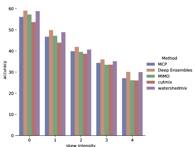
Figure 4: Results on Cityscapes-C dataset’s mIoU for the different level of noise intensity.

8.2 Ablation studies on Superpixels

Our algorithm has two parameters to set: the number of superpixels, and the proportion of selected superpixels used as masks for mixing. In this section we study the impact of the choice of these parameters over the peformance downstream. To this end, we conduct an ablation on Cityscapes over the same split of 744 images.

Our first study is related to the number of superpixels in Superpixel-mix and report results in Table 6. We can see that the performance increases with the number of superpixels up to 200. After this point, the mIoU score decreases. The number of superpixels is directly linked to their size. It is also connected the number of salient edges that will be kept from the original images. Hence, we can deduce that most of the true edges are discarded in the case of a small number of superpixels, leading to low performances. While in the case where we have a high number of superpixels, we might have an over-segmentation that likely leads to a high granularity non-informative masks that prevent learning representations for objects and object parts. In such cases, performance is lower.

Our second study is linked to the proportion of selected superpixels. The results of this survey are in Table 7. We can see that the performance is stable across the range of different values.

Nb. superpixels	20	50	100	200	500	1000
mIoU	63.81 %	64.47%	65.16%	65.0 %	64.16 %	64.2%

Table 6: Ablation study results on the number of superpixels on Cityscapes dataset. All DCNNs are trained on the same split of 1/7 image set under the same conditions.

Proportion	0.1	0.2	0.3	0.4	0.5	0.6	0.7	0.8	0.9
Performance (mIoU)	65.59 %	65.54%	65.43%	65.0%	65.29%	65.63 %	64.9%	65.59	65.41

Table 7: Ablation study results on proportion of chosen superpixels on Cityscapes dataset. All DCNNs are trained on the same split of 1/7 image set under the same conditions.

8.3 Semi-supervised experiments on Pascal

We evaluate our method for semi-supervised semantic segmentation on the Pascal VOC 2012 dataset [Everingham et al.(2012)Everingham, Van Gool, Williams, Winn, and Zisserman]. We compare against top existing methods, following the common protocol from prior works [Hung et al.(2018)Hung, Tsai, Liou, Lin, and Yang, French et al.(2020)French, Laine, Aila, Mackiewicz, and Finlayson], i.e., four sets of labeled data: 1/100 (106 images), 1/50 (212 images), 1/20 (529 images), 1/8 (1323 images). We report results in Table 8. All methods use the same training data split, however, in contrast with prior works that report results only from a single training run, we conduct six different runs to assess the stability of our approach and report mean mIoU scores and standard deviation.

Labeled samples	1/100 (106)	1/50 (212)	1/20 (529)	1/8 (1323)
Adversarial [Hung et al.(2018)Hung, Tsai, Liou, Lin, and Yang]	-	57.2%	64.7%	69.5%
s4GAN [Mittal et al.(2019)Mittal, Tatarchenko, and Brox]	-	63.3%	67.2%	71.4%
Cutout [DeVries and Taylor(2017)]	48.73%	58.26%	64.37%	66.79%
Cutmix [French et al.(2020)French, Laine, Aila, Mackiewicz, and Finlayson]	57,01%	65,99%	68,3%	71,2%
Classmix [Olsson et al.(2020)Olsson, Tranheden, Pinto, and Svensson]	54.18%	66.15%	67.77%	71.00%
DMT[Feng et al.(2020)Feng, Zhou, Cheng, Tan, Shi, and Ma]	61.6%	65.5%	69.3%	70.7%
Baseline(*)	42.47%	55.69%	61.36%	67.14%
Superpixel-mix (ours)	57,69% $\pm$ 0,53 ($\uparrow$ 15.22%)	66,73% $\pm$ 0,54 ($\uparrow$ 11.04%)	69.87% $\pm$ 0,39 ($\uparrow$ 8.51%)	72,04% $\pm$ 0,40 ($\uparrow$ 4.9%)

Table 8: Performance (mIoU) on Pascal VOC 2012 [Everingham et al.(2012)Everingham, Van Gool, Williams, Winn, and Zisserman] on the validation set, which is computed over official split used by [French et al.(2020)French, Laine, Aila, Mackiewicz, and Finlayson]. For Superpixel-mix we report scores averaged over six different runs.

8.4 Semi-supervised experiments on ISIC 2017

We evaluate our method for semi-supervised semantic segmentation on the ISIC skin lesion segmentation dataset [Codella et al.(2018)Codella, Gutman, Celebi, Helba, Marchetti, Dusza, Kalloo, Liopyris, Mishra, Kittler, et al.]. We compare ours against the top existing methods, following the common protocol from prior works [Hung et al.(2018)Hung, Tsai, Liou, Lin, and Yang, French et al.(2020)French, Laine, Aila, Mackiewicz, and Finlayson]. We use 50 out of the 2000 training images and scaled them to $248\times 248$. Then we apply a random crop of $224\times 224$ with random flips and rotations, and uniform scaling in the range from 0.9 to 1.1. We report results in Table 9. The results are averaged on 5 different splits. For this dataset, similarly to  [Hung et al.(2018)Hung, Tsai, Liou, Lin, and Yang, French et al.(2020)French, Laine, Aila, Mackiewicz, and Finlayson, Li et al.(2018)Li, Yu, Chen, Fu, and Heng], we use DenseUNet-161 pretrained on Imagenet.

Labeled samples	(50)
Self ensemble [Li et al.(2018)Li, Yu, Chen, Fu, and Heng]	75.31%
Cutout [DeVries and Taylor(2017)]	68.76%
Cutmix [French et al.(2020)French, Laine, Aila, Mackiewicz, and Finlayson]	74.57%
Baseline(*)	67.64%
Superpixel-mix (ours)	74.53% $\pm$ 1,23 ($\uparrow$ 6.89%)

Table 9: Performance (mIoU) on ISIC skin lesion segmentation dataset [Codella et al.(2018)Codella, Gutman, Celebi, Helba, Marchetti, Dusza, Kalloo, Liopyris, Mishra, Kittler, et al.] on the validation set. The results are averaged over 5 splits.

9 Novel dataset Out of Context Cityscapes (OC-Cityscapes)

In Figure 5, we illustrate a few example images from the contextual free Cityscape dataset used in the unbiaising DCNN experiment. To build this dataset, we replace the pavements and roads with natural landscapes such as sea, forest, desert background. These extreme settings allow to better identify and assess potential contextual biases of semantic segmentation models. The dataset will be made publicly available after the anonymity period.

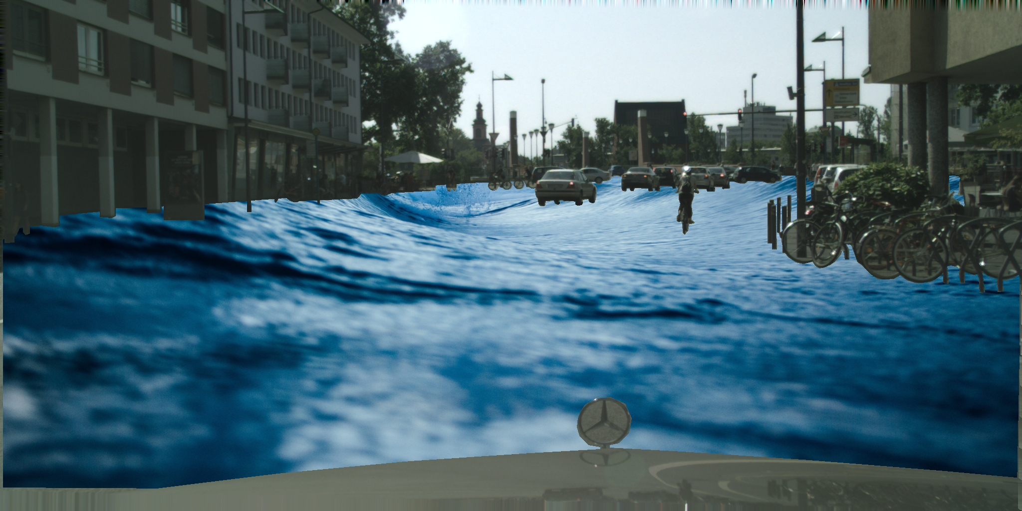
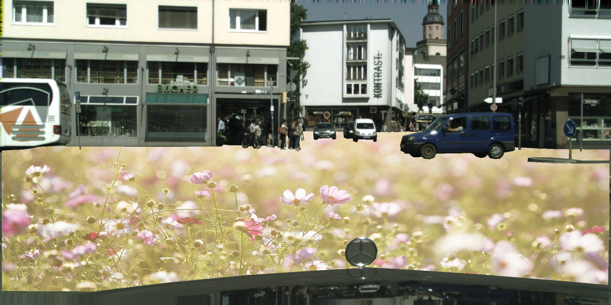
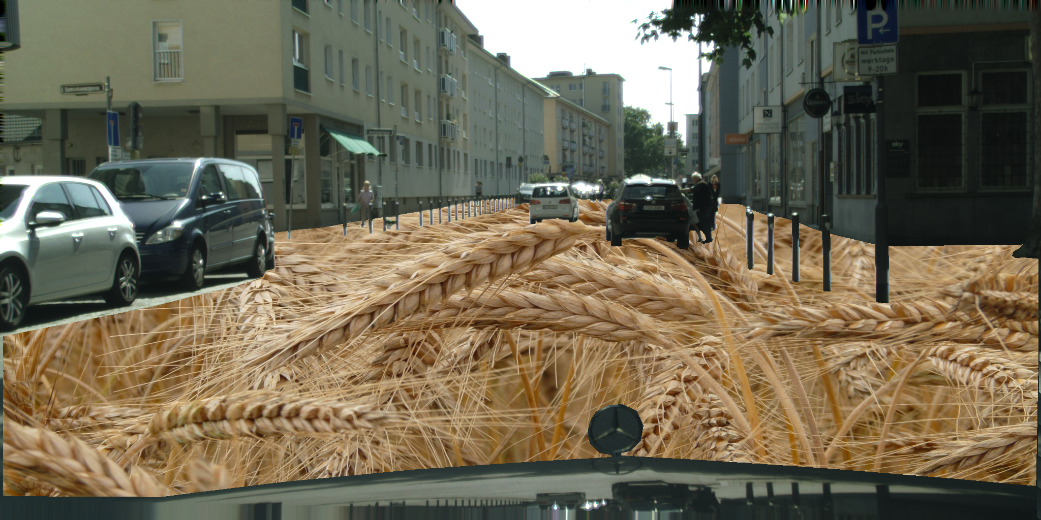
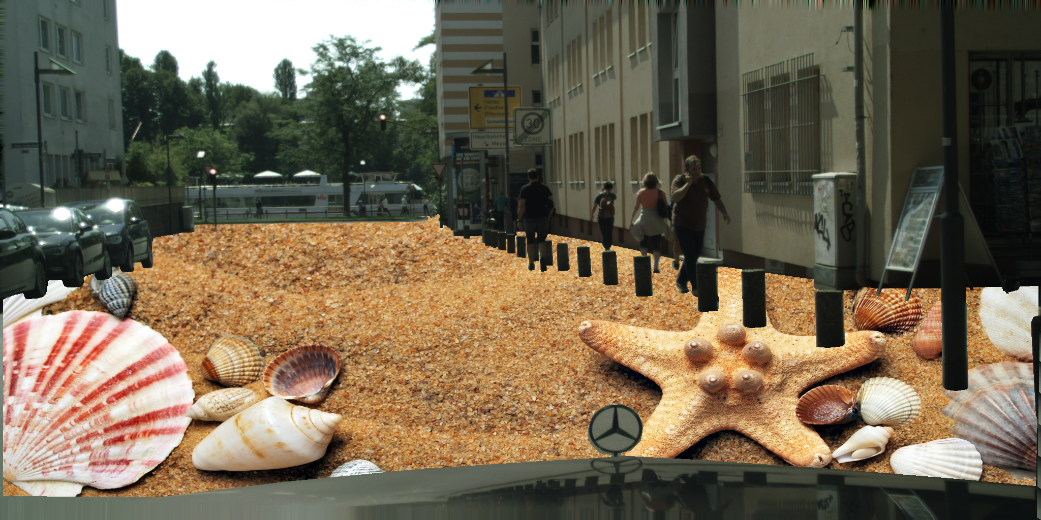
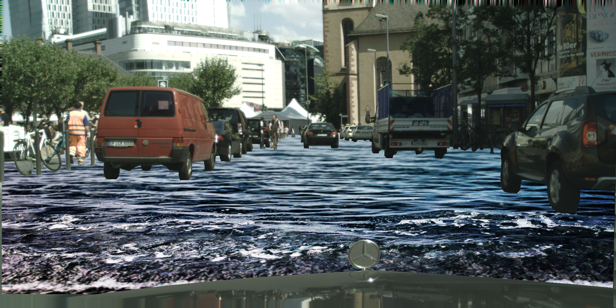
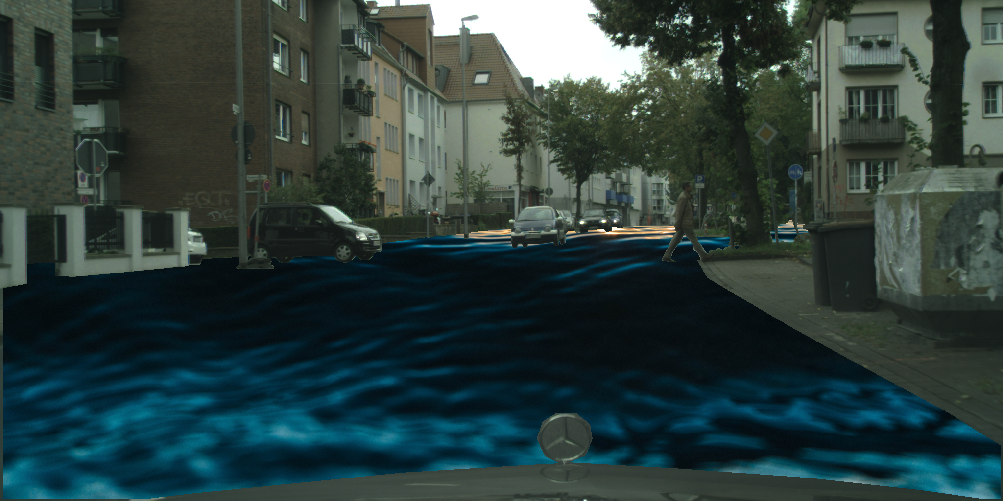
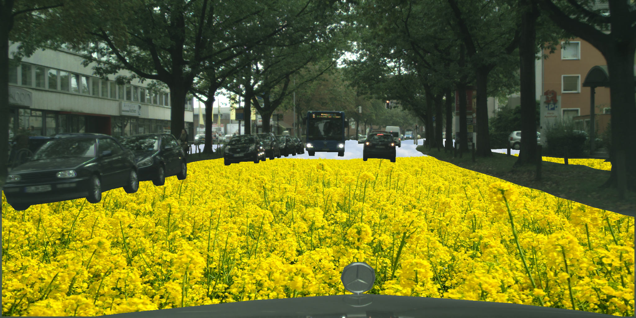
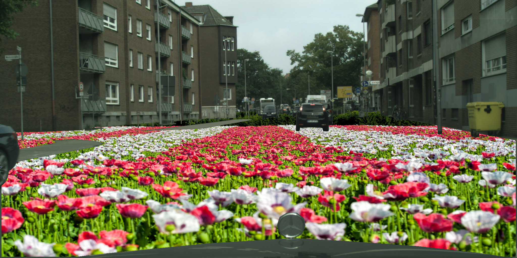
Figure 5: Illustration of some images of OC-Cityscapes dataset

10 Novel dataset Out of Context Cityscapes (OC-Cityscapes)

In Figure 5, we illustrate a few example images from the contextual free Cityscape dataset used in the unbiaising DCNN experiment. To build this dataset, we replace the pavements and roads with natural landscapes such as sea, forest, desert background. These extreme settings allow to better identify and assess potential contextual biases of semantic segmentation models.

11 Implementation details

In this section, we provide the hyper-parameters that are used in the semantic-segmentation experiments. Our code is implemented in PyTorch [Paszke et al.(2019)Paszke, Gross, Massa, Lerer, Bradbury, Chanan, Killeen, Lin, Gimelshein, Antiga, Desmaison, Kopf, Yang, DeVito, Raison, Tejani, Chilamkurthy, Steiner, Fang, Bai, and Chintala]. The code will be made publicly available after the anonymity period.

Hyper-parameter	StreetHazards	Cityscape	ISIC 2017
Architecture	Deeplab v3+	Deeplab v3+	DenseUNet-161
output stride	16	8	-
learning rate	0.1	0.1	0.1
batch size	4	16	8
number of train epochs	25	25	25
weight decay	0.0001	0.0001	0.0001
SyncEnsemble BN	False	False	False
random crop of training images	None	768	224

Table 10: Hyper-parameter configuration used in the fully supervised semantic segmentation experiments .

Hyper-parameter	Cityscape	Pascal
Architecture	Deeplab v2	Deeplab v2
output stride	16	16
learning rate	2.5e-4	2.5e-4
batch size	2	5
number of training iteration	40000	40000
weight decay	5e-4	5e-4
SyncEnsemble BN	True	True

Table 11: Hyper-parameter configuration used in the semi supervised semantic segmentation experiments .

References

- [Achanta et al.(2012)Achanta, Shaji, Smith, Lucchi, Fua, Süsstrunk, et al.] Radhakrishna Achanta, Appu Shaji, Kevin Smith, Aurelien Lucchi, Pascal Fua, Sabine Süsstrunk, et al. SLIC superpixels compared to state-of-the-art superpixel methods. TPAMI, 34, 2012.
- [Ashukha et al.(2020)Ashukha, Lyzhov, Molchanov, and Vetrov] Arsenii Ashukha, Alexander Lyzhov, Dmitry Molchanov, and Dmitry Vetrov. Pitfalls of in-domain uncertainty estimation and ensembling in deep learning. In ICLR, 2020.
- [Berman et al.(2018)Berman, Triki, and Blaschko] Maxim Berman, Amal Rannen Triki, and Matthew B Blaschko. The lovász-softmax loss: A tractable surrogate for the optimization of the intersection-over-union measure in neural networks. In CVPR, 2018.
- [Berthelot et al.(2019a)Berthelot, Carlini, Cubuk, Kurakin, Sohn, Zhang, and Raffel] David Berthelot, Nicholas Carlini, Ekin D Cubuk, Alex Kurakin, Kihyuk Sohn, Han Zhang, and Colin Raffel. Remixmatch: Semi-supervised learning with distribution alignment and augmentation anchoring. arXiv preprint arXiv:1911.09785, 2019a.
- [Berthelot et al.(2019b)Berthelot, Carlini, Goodfellow, Papernot, Oliver, and Raffel] David Berthelot, Nicholas Carlini, Ian Goodfellow, Nicolas Papernot, Avital Oliver, and Colin A Raffel. Mixmatch: A holistic approach to semi-supervised learning. In Advances in Neural Information Processing Systems, pages 5049–5059, 2019b.
- [Berthelot et al.(2019c)Berthelot, Carlini, Goodfellow, Papernot, Oliver, and Raffel] David Berthelot, Nicholas Carlini, Ian Goodfellow, Nicolas Papernot, Avital Oliver, and Colin A Raffel. MixMatch: A holistic approach to semi-supervised learning. In NeurIPS, 2019c.
- [Beucher(1979)] Serge Beucher. Use of watersheds in contour detection. In Proceedings of the International Workshop on Image Processing. CCETT, 1979.
- [Beucher(1994)] Serge Beucher. Watershed, hierarchical segmentation and waterfall algorithm. In Mathematical morphology and its applications to image processing, pages 69–76. Springer, 1994.
- [Beucher and Meyer(1993)] Serge Beucher and Fernand Meyer. The morphological approach to segmentation: the watershed transformation. Mathematical morphology in image processing, 34:433–481, 1993.
- [Brosse et al.(2020)Brosse, Riquelme, Martin, Gelly, and Moulines] Nicolas Brosse, Carlos Riquelme, Alice Martin, Sylvain Gelly, and Éric Moulines. On last-layer algorithms for classification: Decoupling representation from uncertainty estimation. arXiv preprint arXiv:2001.08049, 2020.
- [Chapelle et al.(2001)Chapelle, Weston, Bottou, and Vapnik] Olivier Chapelle, Jason Weston, Léon Bottou, and Vladimir Vapnik. Vicinal risk minimization. Advances in neural information processing systems, pages 416–422, 2001.
- [Chen et al.(2017)Chen, Papandreou, Kokkinos, Murphy, and Yuille] Liang-Chieh Chen, George Papandreou, Iasonas Kokkinos, Kevin Murphy, and Alan L Yuille. Deeplab: Semantic image segmentation with deep convolutional nets, atrous convolution, and fully connected crfs. TPAMI, 40, 2017.
- [Chen et al.(2018)Chen, Zhu, Papandreou, Schroff, and Adam] Liang-Chieh Chen, Yukun Zhu, George Papandreou, Florian Schroff, and Hartwig Adam. Encoder-decoder with atrous separable convolution for semantic image segmentation. In ECCV, 2018.
- [Chen et al.(2020)Chen, Kornblith, Norouzi, and Hinton] Ting Chen, Simon Kornblith, Mohammad Norouzi, and Geoffrey Hinton. A simple framework for contrastive learning of visual representations. In ICML, 2020.
- [Chen and He(2021)] Xinlei Chen and Kaiming He. Exploring simple siamese representation learning. In CVPR, 2021.
- [Codella et al.(2018)Codella, Gutman, Celebi, Helba, Marchetti, Dusza, Kalloo, Liopyris, Mishra, Kittler, et al.] Noel CF Codella, David Gutman, M Emre Celebi, Brian Helba, Michael A Marchetti, Stephen W Dusza, Aadi Kalloo, Konstantinos Liopyris, Nabin Mishra, Harald Kittler, et al. Skin lesion analysis toward melanoma detection: A challenge at the 2017 international symposium on biomedical imaging (isbi), hosted by the international skin imaging collaboration (isic). In 2018 IEEE 15th international symposium on biomedical imaging (ISBI 2018), pages 168–172. IEEE, 2018.
- [Cordts et al.(2016)Cordts, Omran, Ramos, Rehfeld, Enzweiler, Benenson, Franke, Roth, and Schiele] Marius Cordts, Mohamed Omran, Sebastian Ramos, Timo Rehfeld, Markus Enzweiler, Rodrigo Benenson, Uwe Franke, Stefan Roth, and Bernt Schiele. The Cityscapes dataset for semantic urban scene understanding. In CVPR, 2016.
- [Deng et al.(2009)Deng, Dong, Socher, Li, Kai Li, and Li Fei-Fei] J. Deng, W. Dong, R. Socher, L. Li, Kai Li, and Li Fei-Fei. ImageNet: A large-scale hierarchical image database. In CVPR, pages 248–255, 2009.
- [DeVries and Taylor(2017)] Terrance DeVries and Graham W Taylor. Improved regularization of convolutional neural networks with Cutout. arXiv preprint arXiv:1708.04552, 2017.
- [Everingham et al.(2012)Everingham, Van Gool, Williams, Winn, and Zisserman] M. Everingham, L. Van Gool, C. K. I. Williams, J. Winn, and A. Zisserman. The PASCAL Visual Object Classes Challenge 2012 (VOC2012) Results. http://www.pascal-network.org/challenges/VOC/voc2012/workshop/index.html, 2012.
- [Eykholt et al.(2018)Eykholt, Evtimov, Fernandes, Li, Rahmati, Xiao, Prakash, Kohno, and Song] Kevin Eykholt, Ivan Evtimov, Earlence Fernandes, Bo Li, Amir Rahmati, Chaowei Xiao, Atul Prakash, Tadayoshi Kohno, and Dawn Song. Robust physical-world attacks on deep learning models. In CVPR, 2018.
- [Felzenswalb and Huttenlocher(2004)] PF Felzenswalb and DP Huttenlocher. Efficient graph-based image segmentation. International Journal of Computer Vision, 2004.
- [Feng et al.(2020)Feng, Zhou, Cheng, Tan, Shi, and Ma] Zhengyang Feng, Qianyu Zhou, Guangliang Cheng, Xin Tan, Jianping Shi, and Lizhuang Ma. Semi-supervised semantic segmentation via dynamic self-training and classbalanced curriculum. arXiv preprint arXiv:2004.08514, 1(2):5, 2020.
- [Fort et al.(2019)Fort, Hu, and Lakshminarayanan] Stanislav Fort, Huiyi Hu, and Balaji Lakshminarayanan. Deep ensembles: A loss landscape perspective. In arXiv, 2019.
- [Franchi et al.(2020a)Franchi, Bursuc, Aldea, Dubuisson, and Bloch] Gianni Franchi, Andrei Bursuc, Emanuel Aldea, Séverine Dubuisson, and Isabelle Bloch. Tradi: Tracking deep neural network weight distributions. In ECCV, 2020a.
- [Franchi et al.(2020b)Franchi, Bursuc, Aldea, Dubuisson, and Bloch] Gianni Franchi, Andrei Bursuc, Emanuel Aldea, Severine Dubuisson, and Isabelle Bloch. Encoding the latent posterior of bayesian neural networks for uncertainty quantification. arXiv preprint arXiv:2012.02818, 2020b.
- [French et al.(2020)French, Laine, Aila, Mackiewicz, and Finlayson] Geoff French, S. Laine, Timo Aila, M. Mackiewicz, and G. Finlayson. Semi-supervised semantic segmentation needs strong, varied perturbations. In BMVC, 2020.
- [Gal and Ghahramani(2016)] Yarin Gal and Zoubin Ghahramani. Dropout as a bayesian approximation: Representing model uncertainty in deep learning. In ICML, 2016.
- [Gatys et al.(2015)Gatys, Ecker, and Bethge] Leon A. Gatys, Alexander S. Ecker, and Matthias Bethge. A neural algorithm of artistic style. CoRR, abs/1508.06576, 2015.
- [Geirhos et al.(2019)Geirhos, Rubisch, Michaelis, Bethge, Wichmann, and Brendel] Robert Geirhos, Patricia Rubisch, Claudio Michaelis, Matthias Bethge, Felix A. Wichmann, and Wieland Brendel. Imagenet-trained CNNs are biased towards texture: Increasing shape bias improves accuracy and robustness. In ICLR, 2019.
- [Geirhos et al.(2020)Geirhos, Jacobsen, Michaelis, Zemel, Brendel, Bethge, and Wichmann] Robert Geirhos, Jörn-Henrik Jacobsen, Claudio Michaelis, Richard Zemel, Wieland Brendel, Matthias Bethge, and Felix A Wichmann. Shortcut learning in deep neural networks. Nature Machine Intelligence, 2020.
- [Gidaris et al.(2020)Gidaris, Bursuc, Komodakis, Pérez, and Cord] Spyros Gidaris, Andrei Bursuc, Nikos Komodakis, Patrick Pérez, and Matthieu Cord. Learning representations by predicting bags of visual words. In CVPR, 2020.
- [Gneiting and Raftery(2007)] Tilmann Gneiting and Adrian E Raftery. Strictly proper scoring rules, prediction, and estimation. JASA, 102, 2007.
- [Grill et al.(2020)Grill, Strub, Altché, Tallec, Richemond, Buchatskaya, Doersch, Pires, Guo, Azar, et al.] Jean-Bastien Grill, Florian Strub, Florent Altché, Corentin Tallec, Pierre H Richemond, Elena Buchatskaya, Carl Doersch, Bernardo Avila Pires, Zhaohan Daniel Guo, Mohammad Gheshlaghi Azar, et al. Bootstrap your own latent: A new approach to self-supervised learning. In NeurIPS, 2020.
- [Guo et al.(2017)Guo, Pleiss, Sun, and Weinberger] Chuan Guo, Geoff Pleiss, Yu Sun, and Kilian Q Weinberger. On calibration of modern neural networks. In ICML, 2017.
- [Gustafsson et al.(2020)Gustafsson, Danelljan, and Schon] Fredrik K Gustafsson, Martin Danelljan, and Thomas B Schon. Evaluating scalable bayesian deep learning methods for robust computer vision. In CVPRW, 2020.
- [Havasi et al.(2020)Havasi, Jenatton, Fort, Liu, Snoek, Lakshminarayanan, Dai, and Tran] Marton Havasi, Rodolphe Jenatton, Stanislav Fort, Jeremiah Zhe Liu, Jasper Snoek, Balaji Lakshminarayanan, Andrew M Dai, and Dustin Tran. Training independent subnetworks for robust prediction. In arXiv, 2020.
- [He et al.(2016)He, Zhang, Ren, and Sun] Kaiming He, Xiangyu Zhang, Shaoqing Ren, and Jian Sun. Deep residual learning for image recognition. In CVPR, 2016.
- [Hein et al.(2019)Hein, Andriushchenko, and Bitterwolf] Matthias Hein, Maksym Andriushchenko, and Julian Bitterwolf. Why relu networks yield high-confidence predictions far away from the training data and how to mitigate the problem. In CVPR, 2019.
- [Hendrycks and Dietterich(2019)] Dan Hendrycks and Thomas Dietterich. Benchmarking neural network robustness to common corruptions and perturbations. In ICLR, 2019.
- [Hendrycks and Gimpel(2017)] Dan Hendrycks and Kevin Gimpel. A baseline for detecting misclassified and out-of-distribution examples in neural networks. In ICLR, 2017.
- [Hendrycks et al.(2019)Hendrycks, Basart, Mazeika, Mostajabi, Steinhardt, and Song] Dan Hendrycks, Steven Basart, Mantas Mazeika, Mohammadreza Mostajabi, Jacob Steinhardt, and Dawn Song. A benchmark for anomaly segmentation. In arXiv, 2019.
- [Hora(1996)] Stephen C Hora. Aleatory and epistemic uncertainty in probability elicitation with an example from hazardous waste management. Reliability Engineering & System Safety, 54(2-3):217–223, 1996.
- [Hu et al.(2019)Hu, Fu, Zhu, and Heng] Xiaowei Hu, Chi-Wing Fu, Lei Zhu, and Pheng-Ann Heng. Depth-attentional features for single-image rain removal. In CVPR, 2019.
- [Hung et al.(2018)Hung, Tsai, Liou, Lin, and Yang] Wei-Chih Hung, Yi-Hsuan Tsai, Yan-Ting Liou, Yen-Yu Lin, and Ming-Hsuan Yang. Adversarial learning for semi-supervised semantic segmentation. In BMVC, 2018.
- [Jaccard(1912)] Paul Jaccard. The distribution of the flora in the alpine zone. 1. New phytologist, 11(2):37–50, 1912.
- [Joo et al.(2020)Joo, Chung, and Seo] Taejong Joo, Uijung Chung, and Min-Gwan Seo. Being bayesian about categorical probability. In ICML, 2020.
- [Kendall and Gal(2017)] Alex Kendall and Yarin Gal. What uncertainties do we need in bayesian deep learning for computer vision? In NeurIPS, 2017.
- [Kim et al.(2020)Kim, Choo, and Song] Jang-Hyun Kim, Wonho Choo, and Hyun Oh Song. Puzzle mix: Exploiting saliency and local statistics for optimal mixup. In ICML, 2020.
- [Kim et al.(2021)Kim, Choo, Jeong, and Song] Jang-Hyun Kim, Wonho Choo, Hosan Jeong, and Hyun Oh Song. Co-mixup: Saliency guided joint mixup with supermodular diversity. arXiv preprint arXiv:2102.03065, 2021.
- [Lakshminarayanan et al.(2017)Lakshminarayanan, Pritzel, and Blundell] Balaji Lakshminarayanan, Alexander Pritzel, and Charles Blundell. Simple and scalable predictive uncertainty estimation using deep ensembles. In NeurIPS, 2017.
- [Lambert et al.(2020)Lambert, Liu, Sener, Hays, and Koltun] John Lambert, Zhuang Liu, Ozan Sener, James Hays, and Vladlen Koltun. Mseg: a composite dataset for multi-domain semantic segmentation. In CVPR, 2020.
- [Lee et al.(2015)Lee, Purushwalkam, Cogswell, Crandall, and Batra] Stefan Lee, Senthil Purushwalkam, Michael Cogswell, David Crandall, and Dhruv Batra. Why m heads are better than one: Training a diverse ensemble of deep networks. arXiv preprint arXiv:1511.06314, 2015.
- [Li et al.(2019a)Li, Xiong, Fan, and Sun] Hanchao Li, Pengfei Xiong, Haoqiang Fan, and Jian Sun. Dfanet: Deep feature aggregation for real-time semantic segmentation. In CVPR, 2019a.
- [Li et al.(2018)Li, Yu, Chen, Fu, and Heng] Xiaomeng Li, Lequan Yu, Hao Chen, Chi-Wing Fu, and Pheng-Ann Heng. Semi-supervised skin lesion segmentation via transformation consistent self-ensembling model. arXiv preprint arXiv:1808.03887, 2018.
- [Li et al.(2019b)Li, Zhou, Pan, and Feng] Xin Li, Yiming Zhou, Zheng Pan, and Jiashi Feng. Partial order pruning: for best speed/accuracy trade-off in neural architecture search. In CVPR, 2019b.
- [Lin et al.(2014)Lin, Maire, Belongie, Hays, Perona, Ramanan, Dollár, and Zitnick] Tsung-Yi Lin, Michael Maire, Serge Belongie, James Hays, Pietro Perona, Deva Ramanan, Piotr Dollár, and C. Lawrence Zitnick. Microsoft COCO: Common objects in context. In ECCV, 2014.
- [Lin et al.(2017)Lin, Goyal, Girshick, He, and Dollár] Tsung-Yi Lin, Priya Goyal, Ross Girshick, Kaiming He, and Piotr Dollár. Focal loss for dense object detection. In CVPR, 2017.
- [Machairas et al.(2014)Machairas, Decencière, and Walter] V. Machairas, E. Decencière, and T. Walter. Waterpixels: Superpixels based on the watershed transformation. In ICIP, 2014.
- [Machairas et al.(2015)Machairas, Faessel, Cárdenas-Peña, Chabardes, Walter, and Decencière] Vaïa Machairas, Matthieu Faessel, David Cárdenas-Peña, Théodore Chabardes, Thomas Walter, and Etienne Decencière. Waterpixels. TIP, 24, 2015.
- [MacKay(1992)] David JC MacKay. Bayesian methods for adaptive models. PhD thesis, California Institute of Technology, 1992.
- [Maddox et al.(2019)Maddox, Garipov, Izmailov, Vetrov, and Wilson] Wesley Maddox, Timur Garipov, Pavel Izmailov, Dmitry Vetrov, and Andrew Gordon Wilson. A simple baseline for bayesian uncertainty in deep learning. In NeurIPS, 2019.
- [Malinin and Gales(2018)] Andrey Malinin and Mark Gales. Predictive uncertainty estimation via prior networks. In NeurIPS, 2018.
- [Michaelis et al.(2019)Michaelis, Mitzkus, Geirhos, Rusak, Bringmann, Ecker, Bethge, and Brendel] Claudio Michaelis, Benjamin Mitzkus, Robert Geirhos, Evgenia Rusak, Oliver Bringmann, Alexander S Ecker, Matthias Bethge, and Wieland Brendel. Benchmarking robustness in object detection: Autonomous driving when winter is coming. CoRR, abs/1907.07484, 2019.
- [Mittal et al.(2019)Mittal, Tatarchenko, and Brox] S. Mittal, M. Tatarchenko, and T. Brox. Semi-supervised semantic segmentation with high- and low-level consistency. TPAMI, 2019.
- [Neal(1995)] Radford M Neal. Bayesian learning for neural networks. PhD thesis, University of Toronto, 1995.
- [Nguyen et al.(2015)Nguyen, Yosinski, and Clune] A. Nguyen, J. Yosinski, and J. Clune. Deep neural networks are easily fooled: High confidence predictions for unrecognizable images. In CVPR, 2015.
- [Olsson et al.(2020)Olsson, Tranheden, Pinto, and Svensson] Viktor Olsson, Wilhelm Tranheden, Juliano Pinto, and Lennart Svensson. ClassMix: segmentation-based data augmentation for semi-supervised learning. arXiv preprint arXiv:2007.07936, 2020.
- [Ovadia et al.(2019)Ovadia, Fertig, Ren, Nado, Sculley, Nowozin, Dillon, Lakshminarayanan, and Snoek] Yaniv Ovadia, Emily Fertig, Jie Ren, Zachary Nado, David Sculley, Sebastian Nowozin, Joshua V Dillon, Balaji Lakshminarayanan, and Jasper Snoek. Can you trust your model’s uncertainty? evaluating predictive uncertainty under dataset shift. In NeurIPS, 2019.
- [Papernot et al.(2017)Papernot, McDaniel, Goodfellow, Jha, Celik, and Swami] Nicolas Papernot, Patrick McDaniel, Ian Goodfellow, Somesh Jha, Z Berkay Celik, and Ananthram Swami. Practical black-box attacks against machine learning. In ACCCS, 2017.
- [Paszke et al.(2019)Paszke, Gross, Massa, Lerer, Bradbury, Chanan, Killeen, Lin, Gimelshein, Antiga, Desmaison, Kopf, Yang, DeVito, Raison, Tejani, Chilamkurthy, Steiner, Fang, Bai, and Chintala] Adam Paszke, Sam Gross, Francisco Massa, Adam Lerer, James Bradbury, Gregory Chanan, Trevor Killeen, Zeming Lin, Natalia Gimelshein, Luca Antiga, Alban Desmaison, Andreas Kopf, Edward Yang, Zachary DeVito, Martin Raison, Alykhan Tejani, Sasank Chilamkurthy, Benoit Steiner, Lu Fang, Junjie Bai, and Soumith Chintala. Pytorch: An imperative style, high-performance deep learning library. In NeurIPS, 2019.
- [Pei et al.(2017)Pei, Cao, Yang, and Jana] Kexin Pei, Yinzhi Cao, Junfeng Yang, and Suman Jana. Deepxplore: Automated whitebox testing of deep learning systems. In proceedings of the 26th Symposium on Operating Systems Principles, pages 1–18, 2017.
- [Pezzementi et al.(2018)Pezzementi, Tabor, Yim, Chang, Drozd, Guttendorf, Wagner, and Koopman] Zachary Pezzementi, Trenton Tabor, Samuel Yim, Jonathan K Chang, Bill Drozd, David Guttendorf, Michael Wagner, and Philip Koopman. Putting image manipulations in context: Robustness testing for safe perception. In SSRR, 2018.
- [Postels et al.(2019)Postels, Ferroni, Coskun, Navab, and Tombari] Janis Postels, Francesco Ferroni, Huseyin Coskun, Nassir Navab, and Federico Tombari. Sampling-free epistemic uncertainty estimation using approximated variance propagation. In ICCV, pages 2931–2940, 2019.
- [Rosenfeld et al.(2018)Rosenfeld, Zemel, and Tsotsos] Amir Rosenfeld, Richard Zemel, and John K. Tsotsos. The elephant in the room. CoRR, abs/1808.03305, 2018.
- [Sakaridis et al.(2018)Sakaridis, Dai, and Van Gool] Christos Sakaridis, Dengxin Dai, and Luc Van Gool. Semantic foggy scene understanding with synthetic data. IJCV, 126(9):973–992, 2018.
- [Sakaridis et al.(2019)Sakaridis, Dai, and Van Gool] Christos Sakaridis, Dengxin Dai, and Luc Van Gool. Guided curriculum model adaptation and uncertainty-aware evaluation for semantic nighttime image segmentation. In ICCV, 2019.
- [Sensoy et al.(2018)Sensoy, Kaplan, and Kandemir] Murat Sensoy, Lance M Kaplan, and Melih Kandemir. Evidential deep learning to quantify classification uncertainty. In NeurIPS, 2018.
- [Shetty et al.(2019)Shetty, Schiele, and Fritz] R. Shetty, B. Schiele, and M. Fritz. Not using the car to see the sidewalk — quantifying and controlling the effects of context in classification and segmentation. In CVPR, 2019.
- [Sohn et al.(2020)Sohn, Berthelot, Li, Zhang, Carlini, Cubuk, Kurakin, Zhang, and Raffel] Kihyuk Sohn, David Berthelot, Chun-Liang Li, Zizhao Zhang, Nicholas Carlini, Ekin D Cubuk, Alex Kurakin, Han Zhang, and Colin Raffel. Fixmatch: Simplifying semi-supervised learning with consistency and confidence. In NeurIPS, 2020.
- [Srivastava et al.(2020)Srivastava, Hashimoto, and Liang] M. Srivastava, T. Hashimoto, and P. Liang. Robustness to spurious correlations via human annotations. In ICML, 2020.
- [Srivastava et al.(2014)Srivastava, Hinton, Krizhevsky, Sutskever, and Salakhutdinov] Nitish Srivastava, Geoffrey Hinton, Alex Krizhevsky, Ilya Sutskever, and Ruslan Salakhutdinov. Dropout: a simple way to prevent neural networks from overfitting. JMLR, 15, 2014.
- [Sudre et al.(2017)Sudre, Li, Vercauteren, Ourselin, and Cardoso] Carole H Sudre, Wenqi Li, Tom Vercauteren, Sebastien Ourselin, and M Jorge Cardoso. Generalised dice overlap as a deep learning loss function for highly unbalanced segmentations. In Deep learning in medical image analysis and multimodal learning for clinical decision support, pages 240–248. Springer, 2017.
- [Sun et al.(2019)Sun, Zhao, Jiang, Cheng, Xiao, Liu, Mu, Wang, Liu, and Wang] Ke Sun, Yang Zhao, Borui Jiang, Tianheng Cheng, Bin Xiao, Dong Liu, Yadong Mu, Xinggang Wang, Wenyu Liu, and Jingdong Wang. High-resolution representations for labeling pixels and regions. arXiv preprint arXiv:1904.04514, 2019.
- [Szegedy et al.(2013)Szegedy, Zaremba, Sutskever, Bruna, Erhan, Goodfellow, and Fergus] Christian Szegedy, Wojciech Zaremba, Ilya Sutskever, Joan Bruna, Dumitru Erhan, Ian Goodfellow, and Rob Fergus. Intriguing properties of neural networks. CoRR, abs/1312.6199, 2013.
- [Tarvainen and Valpola(2017)] Antti Tarvainen and Harri Valpola. Mean teachers are better role models: Weight-averaged consistency targets improve semi-supervised deep learning results. In NeurIPS, 2017.
- [Van Amersfoort et al.(2020)Van Amersfoort, Smith, Teh, and Gal] Joost Van Amersfoort, Lewis Smith, Yee Whye Teh, and Yarin Gal. Uncertainty estimation using a single deep deterministic neural network. In ICMLR, 2020.
- [Van den Bergh et al.(2012)Van den Bergh, Boix, Roig, de Capitani, and Van Gool] Michael Van den Bergh, Xavier Boix, Gemma Roig, Benjamin de Capitani, and Luc Van Gool. Seeds: Superpixels extracted via energy-driven sampling. In ECCV, 2012.
- [Vasiljevic et al.(2016)Vasiljevic, Chakrabarti, and Shakhnarovich] Igor Vasiljevic, Ayan Chakrabarti, and Gregory Shakhnarovich. Examining the impact of blur on recognition by convolutional networks. arXiv preprint arXiv:1611.05760, 2016.
- [Verma et al.(2019)Verma, Lamb, Beckham, Najafi, Mitliagkas, Lopez-Paz, and Bengio] Vikas Verma, Alex Lamb, Christopher Beckham, Amir Najafi, Ioannis Mitliagkas, David Lopez-Paz, and Yoshua Bengio. Manifold mixup: Better representations by interpolating hidden states. In ICML, 2019.
- [Wen et al.(2020)Wen, Tran, and Ba] Yeming Wen, Dustin Tran, and Jimmy Ba. Batchensemble: an alternative approach to efficient ensemble and lifelong learning. In ICLR, 2020.
- [Xiao et al.(2021)Xiao, Engstrom, Ilyas, and Madry] Kai Xiao, Logan Engstrom, Andrew Ilyas, and Aleksander Madry. Noise or signal: The role of image backgrounds in object recognition. In ICLR, 2021.
- [Yu et al.(2018)Yu, Wang, Peng, Gao, Yu, and Sang] C Yu, J Wang, C Peng, C Gao, G Yu, and N Sang. Bisenet: Bilateral segmentation network for real-time semantic segmentation. In ECCV, 2018.
- [Yu et al.(2017)Yu, Koltun, and Funkhouser] Fisher Yu, Vladlen Koltun, and Thomas Funkhouser. Dilated residual networks. In CVPR, 2017.
- [Yun et al.(2019)Yun, Han, Chun, Oh, Yoo, and Choe] S. Yun, D. Han, S. Chun, S. J. Oh, Y. Yoo, and J. Choe. CutMix: Regularization strategy to train strong classifiers with localizable features. In ICCV, 2019.
- [Zhang et al.(2017)Zhang, Cisse, Dauphin, and Lopez-Paz] Hongyi Zhang, Moustapha Cisse, Yann N Dauphin, and David Lopez-Paz. mixup: Beyond empirical risk minimization. In ICLR, 2017.
- [Zhao et al.(2017)Zhao, Shi, Qi, Wang, and Jia] Hengshuang Zhao, Jianping Shi, Xiaojuan Qi, Xiaogang Wang, and Jiaya Jia. Pyramid scene parsing network. In CVPR, 2017.
- [Zhao et al.(2018)Zhao, Qi, Shen, Shi, and Jia] Hengshuang Zhao, Xiaojuan Qi, Xiaoyong Shen, Jianping Shi, and Jiaya Jia. Icnet for real-time semantic segmentation on high-resolution images. In ECCV, 2018.
- [Zhu et al.(2019)Zhu, Sapra, Reda, Shih, Newsam, Tao, and Catanzaro] Yi Zhu, Karan Sapra, Fitsum A Reda, Kevin J Shih, Shawn Newsam, Andrew Tao, and Bryan Catanzaro. Improving semantic segmentation via video propagation and label relaxation. In CVPR, 2019.