Scope-Bounded Reachability in Valence Systems

Abstract

Multi-pushdown systems are a standard model for concurrent recursive programs, but they have an undecidable reachability problem. Therefore, there have been several proposals to underapproximate their sets of runs so that reachability in this underapproximation becomes decidable. One such underapproximation that covers a relatively high portion of runs is scope boundedness. In such a run, after each push to stack $i$, the corresponding pop operation must come within a bounded number of visits to stack $i$.

In this work, we generalize this approach to a large class of infinite-state systems. For this, we consider the model of valence systems, which consist of a finite-state control and an infinite-state storage mechanism that is specified by a finite undirected graph. This framework captures pushdowns, vector addition systems, integer vector addition systems, and combinations thereof. For this framework, we propose a notion of scope boundedness that coincides with the classical notion when the storage mechanism happens to be a multi-pushdown.

We show that with this notion, reachability can be decided in $\PSPACE$ for every storage mechanism in the framework. Moreover, we describe the full complexity landscape of this problem across all storage mechanisms, both in the case of (i) the scope bound being given as input and (ii) for fixed scope bounds. Finally, we provide an almost complete description of the complexity landscape if even a description of the storage mechanism is part of the input.

1 Introduction

Multi-pushdown systems are a natural model for recursive programs with threads that communicate via shared memory. Unfortunately, even safety verification (state reachability) is undecidable for this model [22]. However, by considering underapproximations of the set of all executions, it is still possible to discover safety violations. The first such underapproximation in the literature was bounded context switching [21]. Here, one only considers executions that switch between threads a bounded number of times. In terms of multi-pushdown systems, this places a bound on the number of times we can switch between stacks.

One underapproximation that covers a relatively large portion of all executions and still permits decidable reachability is scope-boundedness as proposed by La Torre, Napoli, and Parlato [25, 27]. Here, instead of bounding the number of context switches across the entire run, we bound the number of context switches per letter on a stack (i.e. procedure execution). More precisely, whenever we push a letter on some stack $i$, then we can switch back to stack $i$ at most $k$ times before we have to pop that letter again. This higher coverage of runs comes at the cost of higher complexity: While reachability with bounded context switching is $\NP$-complete [12, 21], the scope-bounded reachability problem is $\PSPACE$-complete (if the number of pushdowns or the scope bound is part of the input) [27].

Aside from multi-pushdown systems, there is a wide variety of other infinite-state models that are used to model program behaviours. For these, reachability problems are also sometimes undecidable or have prohibitively high complexity. For example, vector addition systems with states (VASS) is one of the most prominent models for concurrent systems, but its reachability problem has non-elementary complexity [8]. This raises the question of whether underapproximations for multi-pushdown systems can be interpreted in other infinite-state systems and what complexity would ensue.

The notion of bounded context switching has recently been generalized to a large class of infinite-state systems [20], in the framework of valence systems over graph monoids. These consist of a finite-state control that has access to a storage mechanism. The shape of this storage mechanism is described by a finite, undirected graph. By choosing an appropriate graph, one can realize many infinite-state models. Examples include (multi-)pushdown systems, VASS, integer VASS, but also combinations thereof, such as pushdown VASS [17] and sequential recursive Petri nets [16]. Under this notion, bounded context reachability is in $\NP$ for each graph, and thus each storage mechanism in the framework [20]. Moreover, the paper [20] presents some subclasses of graphs for which bounded context reachability has lower complexity ($\NL$ or $\P$). However, the exact complexity of reachability under bounded context switching remains open in many cases, such as the path with four nodes [20].

Contribution We present an abstract notion of scope-bounded runs for valence systems over graph monoids. As we show, this notion always leads to a reachability problem decidable in $\PSPACE$. In particular, our notion applies to all infinite-state models mentioned above. Moreover, applied to multi-pushdown systems, it coincides with the notion of La Torre, Napoli, and Parlato.

We also obtain an almost complete complexity landscape of scope-bounded reachability. First, we show that if both (i) the graph $\Gamma$ describing the storage mechanism and (ii) the scope bound $k$ are part of the input, the problem is $\PSPACE$-complete. Second, we study how the complexity depends on the employed storage mechanism. We show that for each $\Gamma$, the problem is either $\NL$-complete, $\P$-complete, or $\PSPACE$-complete, depending on $\Gamma$ (Corollary 4.2). Since the complexity drops below $\PSPACE$ only in extremely restricted cases, we also study the setting where the scope bound $k$ is fixed. In this case, we show that the problem is either $\NL$-complete or $\P$-complete, depending on $\Gamma$ (Corollary 4.4).

Finally, applying scope-boundedness to classes of infinite-state systems requires understanding the complexity if $\Gamma$ is drawn from an infinite class of graphs. For example, for each fixed dimension $d$, there is a graph $\Gamma_{d}$ such that valence automata over $\Gamma_{d}$ correspond to VASS of dimension $d$. The class of all VASS (of arbitrary dimension), however, corresponds to valence automata over all cliques. Thus, we also study scope-bounded reachability if $\Gamma$ is restricted to a class of graphs $\mathcal{G}$. Under a mild assumption on $\mathcal{G}$, we again obtain a complexity trichotomy of $\NL$-, $\P$-, or $\PSPACE$-completeness, both for $k$ as input (Theorem 4.1) and for fixed $k$ (Theorem 4.3). In fact, all results mentioned above follow from these general results.

Related work Similar in spirit to our work are the lines of research on systems with bounded tree-width by Madhusudan and Parlato [19] and on bounded split-width by Aiswarya [6]. In these settings, the storage mechanism is represented as a class of possible matching relations on the positions of a computation. Then, under the assumption that the resulting behavior graphs have bounded tree-width or split-width, respectively, there are general decidability results. In particular, decidability of scope-bounded reachability in multi-pushdown systems has been deduced via tree-width [28] and via split-width [7]. Different from underapproximations based on bounded tree-width or split-width, our framework includes multi-counter systems (such as VASS or integer VASS), but also counters nested in stacks. While VASS can be seen as special cases of multi-pushdown systems, our framework allows us, e.g. to study the complexity of scope-bounded reachability if the storage mechanism is restricted to multi-counters. On the other hand, while tree-width and split-width can be considered for queues [19, 1], they cannot be realized as storage mechanisms in valence systems.

Furthermore, after their introduction [25] scope-bounded multi-pushdown systems have been studied in terms of accepted languages [26], temporal logic model checking [28, 3]. Moreover, scope-boundedness has been studied in the timed setting [2],[4].

Over the last decade, the framework of valence automata over graph monoids has been used to study how several types of analysis are impacted by the choice of storage mechanism. For example: For which storage mechanisms (i) can silent transitions be algorithmically eliminated? [29]; (ii) do we have a Parikh’s theorem [5], (iii) is (general) reachability decidable [33]; (iv) is first-order logic with reachability decidable? [10]; (v) can downward closures be computed effectively? [30].

Details of all proofs can be found in the full version of the paper.

2 Preliminaries

In this section, we recall the basics of valence systems over graph monoids [31].

Graph Monoids This class of monoids accommodate a variety of storage mechanisms. They are defined by undirected graphs without parallel edges $\Gamma=(V,I)$ where $V$ is a finite set of vertices and $I\subseteq\{e\subseteq V\mid 1\leq|e|\leq 2\}$ is a finite set of undirected edges, which can be self-loops. Thus, if $\{v\}\in I$, we say that $v$ is looped; otherwise, $v$ is unlooped. The edge relation is also called an independence relation. We also write $uIv$ for $\{u,v\}\in I$. A subset $U\subseteq V$ is a clique if $uIv$ for any two distinct $u,v\in U$. If in addition, all $v\in U$ are looped, then $U$ is a looped clique. If $U$ is a clique and all $v\in U$ are unlooped, then $U$ is an unlooped clique. We say that $U\subseteq V$ is an anti-clique if we do not have $uIv$ for any distinct $u,v\in U$. Given the graph, we define a monoid as follows. We have the alphabet $X_{\Gamma}=\{v^{+},v^{-}\mid v\in V\}$, where we write $xIy$ for $x,y\in X_{\Gamma}$ if for some $u,v\in V$, we have $x\in\{u^{+},u^{-}\}$, $y\in\{v^{+},v^{-}\}$, $x\neq y$, and $uIv$. Moreover, $\equiv_{\Gamma}$ is the smallest congruence on $X_{\Gamma}^{*}$ with $v^{+}v^{-}\equiv_{\Gamma}\varepsilon$ for $v\in V$ and $xy\equiv_{\Gamma}yx$ for $xIy$. Here, $\varepsilon$ denotes the empty word. Thus, if $v$ has a self-loop, then $v^{-}v^{+}\equiv_{\Gamma}\varepsilon$. We define the monoid $\mathbb{M}\Gamma:=X_{\Gamma}^{*}/\equiv_{\Gamma}$.

Valence Systems Graph monoids are used in valence systems, which are finite automata whose edges are labeled with elements of a monoid. Then, a run is considered valid if the product of the monoid elements is the neutral element. Here, we only consider the case where the monoid is of the form $\mathbb{M}\Gamma$, so we define the concept directly for graphs.

Given a graph $\Gamma$, a valence system $\mathcal{A}$ over $\Gamma$ consists of a finite set of states $Q$, and a transition relation $\rightarrow\subseteq Q\times X_{\Gamma}^{*}\times Q$. A configuration of $\mathcal{A}$ is a tuple $(q,w)$ where $q\in Q$, $w\in X_{\Gamma}^{*}$ is the sequence of storage operations executed so far. From a configuration $(q_{1},u)$, on a transition $q_{1}\stackrel{{\scriptstyle v}}{{\rightarrow}}q_{2}$, we reach the configuration $(q_{2},uv)$. A run of $\mathcal{A}$ is a sequence of transitions. The reachability problem in valence systems is the following: Given states $q_{\mathit{init}}$ and $q_{\mathit{fin}}$, is there a run from $(q_{\mathit{init}},\varepsilon)$ that reaches $(q_{\mathit{fin}},w)$ for some $w\in X_{\Gamma}^{*}$ with $w\equiv_{\Gamma}\varepsilon$?

Many classical storage types can be realized with graph monoids. Consider $\bar{\Gamma}_{3}=(V,I)$ in Figure 1. We have $I=\{\{a,c\},\{b,c\},\{c\}\}$. For $w\in X_{\bar{\Gamma}_{3}}^{*}$ we have $w\equiv_{\bar{\Gamma}_{3}}\varepsilon$ if and only if two conditions are met: First, if we project to $\{a^{+},a^{-},b^{+},b^{-}\}$, then the word corresponds to a sequence of push- and pop-operations that transform the empty stack into the empty stack. Here, $x^{+}$ corresponds to pushing $x$, and $x^{-}$ to popping $x$, for $x\in\{a,b\}$. Second, the number of $c^{+}$ is the same as the number of $c^{-}$ in $w$. Thus, valence automata over $\bar{\Gamma}_{3}$ can be seen as pushdown automata that have access to a $\mathbb{Z}$-valued counter. Similarly, the storage mechanism of $\Gamma_{2}$ in Figure 1 is a stack, where each stack entry is not a letter, but contains two $\mathbb{N}$-valued counters. A push ($c^{+}$) starts a new stack entry and a pop ($c^{-}$) is only possible if the topmost two counters are zero. For more examples and explanation, see [32].

Example 2.1 (Example storage mechanisms).

Let us mention a few particular (classes of) graphs and how they correspond to infinite-state systems. In the following, the direct product of two graphs $\Gamma$ and $\Delta$ is the graph obtained by taking the disjoint union of $\Gamma$ and $\Delta$ and adding an edge between each vertex from $\Gamma$ and each vertex from $\Delta$.

Pushdown

For $s\in\mathbb{N}$, let $\mathsf{P}_{s}$ be the graph on $s$ vertices without edges. Then valence automata over $\mathsf{P}_{s}$ correspond to pushdown systems with $s$ stack symbols.

Multi-pushdown

Let $\mathsf{MP}_{r,s}$ be the direct product of $r$ disjoint copies of $\mathsf{P}_{s}$. Then valence systems over $\mathsf{MP}_{r,s}$ correspond to multi-pushdown systems with $r$ stacks, each of which has $s$ stack symbols. In Figure 1, the induced subgraph of graph $\Gamma_{1}$ on $\{b_{1},b_{2},b_{3},c_{1},c_{2},c_{3}\}$ represents $\mathsf{MP}_{2,3}$.

VASS

If $\mathsf{UC}_{d}$ is an unlooped clique with $d$ vertices, then valence systems over $\mathsf{UC}_{d}$ correspond to $d$-dimensional vector addition systems with states.

Integer VASS

If $\mathsf{LC}_{d}$ be a looped clique with $d$ vertices, then valence systems over $\mathsf{LC}_{d}$ correspond to $d$-dimensional integer VASS.

Pushdown VASS

If $\mathsf{UC}^{-}_{d}$ is the graph obtained from $\mathsf{UC}_{d+2}$ by removing a single edge, then valence systems over $\mathsf{UC}^{-}_{d}$ correspond to $d$-dimensional pushdown VASS.

3 Scope-bounded runs in valence systems

In this section, we introduce our notion of bounded scope to valence systems over arbitrary graph monoids. For each of the used concepts, we will explain how they relate to the existing notion of scope-boundedness for multi-pushdown systems. Fixing $\Gamma=(V,I)$ as before, first we introduce some preliminary notations and definitions.

Dependent sets and contexts Recall that valence systems over the graph $\mathsf{MP}_{r,s}$ realize a storage consisting of $r$ pushdowns, each with $s$ stack symbols. The graph $\mathsf{MP}_{r,s}$ is a direct product of $r$-many disjoint anti-cliques, each with $s$ vertices. Here, each anti-clique corresponds to a pushdown with $s$ stack symbols: For a vertex $v$ in such an anti-clique, the symbol $v^{+}$ is the push operation for this stack symbol, and $v^{-}$ is its pop operation.

In a multi-pushdown system, a run is naturally decomposed into contexts, where each context is a sequence of operations belonging to one stack. In [20], the notion of context was generalized to valence systems as follows. A set $U\subseteq V$ is called dependent if it does not contain distinct vertices $u_{1},u_{2}\in V$ such that $u_{1}Iu_{2}$. A set of operations $Y\subseteq X_{\Gamma}$ is dependent if its underlying set of vertices $\{v\in V\mid v^{+}\in Y$ or $v^{-}\in Y\}$ is dependent. A computation is called dependent if the set of operations occurring in it is dependent. A dependent computation is also called a context. In $\Gamma_{1}$ of Figure 1, contexts can be formed over $\{b_{1},b_{2},b_{3}\}$, $\{c_{1},c_{2},c_{3}\}$ and $\{a\}$.

Context decomposition Note that a word $w\in X_{\Gamma}^{*}$ need not have a unique decomposition into contexts. For example, for $\Gamma_{2}$ in Figure 1, the word $a^{+}c^{+}b^{+}$ can be decomposed as $(a^{+}c^{+})b^{+}$ and as $a^{+}(c^{+}b^{+})$. Therefore, we now define a canonical decomposition into contexts, which decomposes the word from left to right. Formally, the canonical context decomposition of a computation $w\in X_{\Gamma}^{+}$ (that is, $|w|>0$) is defined inductively. If $w$ is over a dependent set of operations, then $w$ is a single context. Otherwise, find the maximal, non-empty prefix $w_{1}$ of $w$ over a dependent set of operations. The canonical decomposition of $w$ into contexts is then $w=w_{1}w_{2}\dots w_{m}$ where $w_{2}\dots w_{m}$ is the decomposition of the remaining word into contexts. In the following, when we mention the contexts of a word, we always mean those in the canonical decomposition. Observe that in the case of $\mathsf{MP}_{r,s}$, this is exactly the decomposition into contexts of multi-pushdown systems.

Reductions. Given a computation $w=x_{1}\dots x_{n}$ where each $x_{i}\in X_{\Gamma}$, we identify each operation $x_{i}$ with its position. We denote by $w[i]$ the $i$th operation of $w$. A reduction of $w$ is a finite sequence of applications of the following rewriting rules that transform $w$ into $\varepsilon$.

(R1) $w^{\prime}.w[x].w[y].w^{\prime\prime}\mapsto_{red}w^{\prime}w^{\prime\prime}$, applicable if $w[x]=o^{+},w[y]=o^{-}$ for some $o$.

(R2) $w^{\prime}.w[x].w[y].w^{\prime\prime}\mapsto_{red}w^{\prime}w^{\prime\prime}$, applicable if $w[x]=o^{-},w[y]=o^{+}$ for some $oIo$.

(R3) $w^{\prime}.w[x].w[y].w^{\prime\prime}\mapsto_{red}w^{\prime}w[y]w[x]w^{\prime\prime}$, applicable if $w[x]Iw[y]$.

Reducing a word $u$ to a word $v$ using these rules is denoted by $u\stackrel{{\scriptstyle*}}{{\mapsto_{red}}}v$. A reduction of $w=a_{1}\dots a_{n}\in X_{\Gamma}^{*}$ to $\varepsilon$ is the same as the free reduction of the sequence $a_{1},a_{2},\dots,a_{n}$. For any computation $w\in X_{\Gamma}^{*}$, we have $w\equiv_{\Gamma}\varepsilon$ iff $w$ admits a reduction to $\varepsilon$ [31, Equation (8.2)].

Assume that $\pi=w\stackrel{{\scriptstyle*}}{{\mapsto_{red}}}\varepsilon$ is a reduction that transforms $w$ into $\varepsilon$. The relation $R_{\pi}$ relates positions of $w$ which cancel in $\pi$.

$$w[x]R_{\pi}w[y]\leavevmode\nobreak\ \leavevmode\nobreak\ \text{if}\leavevmode\nobreak\ \leavevmode\nobreak\ w^{\prime}.w[x].w[y].w^{\prime\prime}\mapsto_{red}w^{\prime}.w^{\prime\prime}\leavevmode\nobreak\ \leavevmode\nobreak\ \text{or}\leavevmode\nobreak\ \leavevmode\nobreak\ w^{\prime}.w[y].w[x].w^{\prime\prime}\mapsto_{red}w^{\prime}.w^{\prime\prime}\leavevmode\nobreak\ \leavevmode\nobreak\ \text{is used in}\leavevmode\nobreak\ \leavevmode\nobreak\ \pi$$

This is inductively lifted to infixes of $w$ as $t_{1}s_{1}R_{\pi}s_{2}t_{2}$ if there are contexts $w_{i}=w_{i1}.t_{1}.s_{1}.w_{i2}$ and $w_{j}=w_{j1}.s_{2}.t_{2}.w_{j2}$ of $w$ such that $s_{1}R_{\pi}s_{2}$ and $t_{1}R_{\pi}t_{2}$.

Greedy reductions A word $w\in X_{\Gamma}^{*}$ is called irreducible if neither of the rules R1 and R2 is applicable in $w$. A reduction $\pi\colon w\stackrel{{\scriptstyle*}}{{\mapsto_{red}}}\varepsilon$ is called greedy if it begins with a sequence of applications of R1 and R2 for each context so that the resulting context is irreducible. Note that every word $w$ with $w\equiv_{\Gamma}\varepsilon$ has a greedy reduction: One can first (greedily) apply R1 and R2 until each context is irreducible. Since the resulting word $w^{\prime}$ still satisfies $w^{\prime}\equiv_{\Gamma}\varepsilon$, there exists a reduction $w^{\prime}\stackrel{{\scriptstyle*}}{{\mapsto_{red}}}\varepsilon$. In total, this yields a greedy reduction.

Figure 1: The storage mechanism of $\Gamma_{1}$ is 2 stacks and one partially blind counter. Symbols of the same stack are weakly dependent. In the storage mechanism of $\Gamma_{2}$, $a,b,c$ are weakly dependent.

Weak dependence In the case of $\Gamma=\mathsf{MP}_{r,s}$, we know that any two vertices $u,v$ are either dependent (i.e. belong to the same pushdown) or $\Gamma$ is the direct product of graphs $\Gamma_{u}$ and $\Gamma_{v}$ such that $u$ belongs to $\Gamma_{u}$ and $v$ belongs to $\Gamma_{v}$. This means, two operations that are not dependent can, inside every computation, be moved past each other without changing the effect on the stacks. This is not the case in general graphs. In $\Gamma_{2}$ in Figure 1, the vertices $a$ and $b$ are not dependent, but in the computation $acb$, they cannot be moved past each other, because none of them commutes with $c$. We therefore need the additional notion of weak dependence. We say that two vertices $u,v\in V$ are weakly dependent if there is a path between them in the complement of the graph. Here, the complement of a graph $\Gamma=(V,I)$ is obtained by complementing the independence relation ($v_{1}Iv_{2}$ in $\Gamma$ iff we do not have $v_{1}Iv_{2}$ in the complement of $\Gamma$). Equivalently, $u$ and $v$ are not weakly dependent if $\Gamma$ is the direct product of graphs $\Gamma_{u}$ and $\Gamma_{v}$ such that $u$ belongs to $\Gamma_{u}$ and $v$ belongs to $\Gamma_{v}$. As observed above, $\Gamma_{2}$ shows that in general, weakly dependent vertices need not be dependent.

It can be seen that weak dependence is an equivalence relation on the set of vertices $V$, where the equivalence classes are the connected components in the complement of $\Gamma$. Note that all operations inside a context must belong to the same weak dependence class. We therefore say that two contexts $c_{1},c_{2}$ are weakly dependent if their operations belong to the same weakly dependent equivalence class. Equivalently, two contexts are weakly dependent if all their letters are pairwise weakly dependent. In particular, weak dependency is an equivalence relation on contexts also. Let us denote the weak dependence equivalence relation by $\sim_{W}$ and by $[\leavevmode\nobreak\ ]_{\sim_{W}}$ the set of all equivalence classes induced by $\sim_{W}$.

Scope bounded runs We now define the notion of bounded scope computations. We first phrase the classical notion of scope-boundedness [27] in our framework. If $\Gamma=\mathsf{MP}_{r,s}$, then $w\in X_{\Gamma}^{*}$ is considered $k$-scope bounded if there is a reduction $\pi$ for $w$ such that in between any two symbols $w[i]$ and $w[j]$ related in $R_{\pi}$, at most $k$ contexts visit the same anti-clique of $w[i]$ and $w[j]$. Note that in $\mathsf{MP}_{r,s}$, for every reduction, there is a greedy reduction that induces the same relation $R_{\pi}$. Indeed, any applications of R1 and R2 that are applicable in a context at the start will eventually be made anyway: In $\mathsf{MP}_{r,s}$, if a word reduces to $\varepsilon$, then every position has a uniquely determined “partner position” with which is cancels in every possible reduction. Therefore, we generalize scope boundedness as follows.

Definition 3.1 (Scope Bounded Computations).

Consider a computation $w\in X_{\Gamma}^{+}$. We say $w$ is $k$-scoped if there is a greedy reduction $\pi=w\stackrel{{\scriptstyle*}}{{\mapsto_{\mathit{red}}}}\varepsilon$ such that in between any two symbols $w[i]$ and $w[j]$ related by $R_{\pi}$, at most $k-1$ contexts between $w[i]$ and $w[j]$ belong to the same weak dependence class as $w[i]$ and $w[j]$.

By $\mathsf{sc}(w)$, we denote the smallest number $k$ so that $w$ is $k$-scoped. Note that there is such a $k$ if and only if $w\equiv_{\Gamma}\varepsilon$. Thus, if $w\not\equiv_{\Gamma}\varepsilon$, we set $\mathsf{sc}(w)=\infty$. In the example in Figure 1 (graph $\Gamma_{1}$) the computation $w={\color[rgb]{0,1,0}b_{1}^{+}}({\color[rgb]{.5,0,.5}c_{2}^{+}}{\color[rgb]{1,0,0}a^{+}}{\color[rgb]{.5,0,.5}c_{1}^{+}}{\color[rgb]{1,0,0}a^{+}}{\color[rgb]{.5,0,.5}c_{1}^{-}}{\color[rgb]{1,0,0}a^{-}}{\color[rgb]{.5,0,.5}c_{2}^{-}}{\color[rgb]{1,0,0}a^{-}})^{m}{\color[rgb]{0,1,0}b_{1}^{-}}$ is 3 scope bounded for all values of $m$, even though the number of context switches grows with $m$.

Interaction distance. We make the notion of scope bound more formal using the notion of interaction distance. Given a computation $w\in X_{\Gamma}^{+}$. Let $c_{1}c_{2}\dots c_{n}$ be the canonical decomposition of $w$ into contexts. We say that two contexts $c_{i},c_{j}$ with $i<j$ have an interaction distance $K$ if there are $K-1$ contexts between $c_{i}$ and $c_{j}$ which are weakly dependent with $c_{i}$. Consider the computation ${\color[rgb]{0,1,0}b_{1}^{+}}({\color[rgb]{1,0,0}a^{+}}{\color[rgb]{.5,0,.5}c_{1}^{+}})^{m_{1}}{\color[rgb]{0,1,0}b_{2}^{+}}({\color[rgb]{1,0,0}a^{+}}{\color[rgb]{.5,0,.5}c_{2}^{+}})^{m_{2}}{\color[rgb]{0,1,0}b_{3}^{+}}({\color[rgb]{1,0,0}a^{+}}{\color[rgb]{.5,0,.5}c_{3}^{+}})^{m_{3}}{\color[rgb]{0,1,0}b_{3}^{-}}({\color[rgb]{.5,0,.5}c_{3}^{-}}{\color[rgb]{1,0,0}a^{-}})^{m_{3}}{\color[rgb]{0,1,0}b_{2}^{-}}({\color[rgb]{.5,0,.5}c_{2}^{-}}{\color[rgb]{1,0,0}a^{-}})^{m_{2}}{\color[rgb]{0,1,0}b_{1}^{-}}({\color[rgb]{.5,0,.5}c_{1}^{-}}{\color[rgb]{1,0,0}a^{-}})^{m_{1}}$. Each differently colored sequence is a context. The interaction distance between ${\color[rgb]{0,1,0}b_{1}^{+}}$ and ${\color[rgb]{0,1,0}b_{1}^{-}}$ is 5, since the weakly dependent contexts strictly between them are ${\color[rgb]{0,1,0}b_{2}^{+}},{\color[rgb]{0,1,0}b_{3}^{+}},{\color[rgb]{0,1,0}b_{3}^{-}},{\color[rgb]{0,1,0}b_{2}^{-}}$.

Thus, $w$ is $k$-scoped if and only if there is a greedy reduction $\pi\colon w\mapsto_{\mathit{red}}\varepsilon$ such that whenever $w[i]R_{\pi}w[j]$, then the contexts of $w[i]$ and $w[j]$ have interaction distance at most $k$.

The following is the central decision problem studied in this paper.

The Bounded Scope Reachability Problem($\mathsf{BSREACH}$) Given: Graph $\Gamma$, scope bound $k$, valence system $\mathcal{A}$ over $\Gamma$, initial state $q_{\mathit{init}}$, final state $q_{\mathit{fin}}$ Decide: Is there a run from $(q_{\mathit{init}},\varepsilon)$ to $(q_{\mathit{fin}},w)$, for some $w\in X_{\Gamma}^{*}$ with $\mathsf{sc}(w)\leq k$?

Thus, in $\mathsf{BSREACH}$, both $\Gamma$ and $k$ are part of the input. We also consider versions where certain parameters are fixed: If $\Gamma$ is fixed, we denote the problem by $\mathsf{BSREACH}(\Gamma)$. If $\Gamma$ is part of the input, but can be drawn from a class $\mathcal{G}$ of graphs, we write $\mathsf{BSREACH}(\mathcal{G})$. Finally, if we fix $k$, we use a subscript $k$, resulting in the problems $\mathsf{BSREACH}_{k}$, $\mathsf{BSREACH}_{k}(\Gamma)$, $\mathsf{BSREACH}_{k}(\mathcal{G})$.

Deciding whether there is a run $(q_{\mathit{init}},\varepsilon)$ to $(q_{\mathit{fin}},w)$ with $w\equiv_{\Gamma}\varepsilon$ corresponds to general configuration reachability [30]. Hence, we consider the scope-bounded version of configuration reachability.

Strongly Induced Subgraphs. When we study decision problems for valence systems over graph monoids, then typically, if $\Delta$ is an induced subgraph of $\Gamma$, then a problem instance for $\Delta$ can trivially be reduced to an instance over $\Gamma$. Here, induced subgraph means that $\Delta$ can be embedded into $\Gamma$ so that there is an edge in $\Delta$ iff there is one in $\Gamma$.

This is not necessarily the case for $\mathsf{BSREACH}$: An induced subgraph might decompose into different weak dependence classes than $\Gamma$. Therefore, we use a stronger notion of embedding. We say that $\Gamma^{\prime}=(V^{\prime},I^{\prime})$ is a strongly induced subgraph of $\Gamma=(V,I)$ if there is an injective map $\iota\colon V\to V^{\prime}$ such that for any $u,v\in V$, we have (i) $uIv$ iff $\iota(u)I^{\prime}\iota(v)$ and (ii) $u\sim_{W}v$ iff $\iota(u)\sim_{W}\iota(v)$. For example, the graph $\Gamma$ consisting of two adjacent vertices (without loops) is an induced subgraph of $\Gamma_{2}$ in Figure 1. However, $\Gamma$ is not a strongly induced subgraph of $\Gamma_{2}$: In $\Gamma_{2}$, $a$ and $b$ are weakly dependent, whereas the vertices of $\Gamma$ are not.

Neighbor Antichains Let $\Gamma=(V,I)$ be a graph. In our algorithms, we will need to store information about a dependent set $U\subseteq V$ from which we can conclude whether for another dependent set $U^{\prime}\subseteq V$, we have $UIU^{\prime}$; that is, for all $u\in U,u^{\prime}\in U^{\prime},uIu^{\prime}$. To estimate the required information, we use the notion of neighbor antichains. Let $\Gamma=(V,I)$ be a graph. Given $v\in V$, let $N(v)$ represent the neighbors of $v$, that is $N(v)=\{u\in V\mid uIv\}$. We define a quasi-ordering on $V$ as follows. For $u,v\in V$, we have $u\leq v$ if $N(u)\subseteq N(v)$. It is possible that for distinct, $u,v\in V$ we have $u\leq v$ and $v\leq u$ and thus $\leq$ is not necessarily a partial order. In the following, we will assume that the graphs $\Gamma$ are always equipped with some linear order $\ll$ on $V$. For example, one can just take the order in which the vertices appear in a description of $\Gamma$. Using $\ll$, we can turn $\leq$ into a partial order, which is easier to use algorithmically: We set $u\preceq v$ if and only if $u\leq v$ and $u\ll v$.

Now, given $U\subseteq V$, let ${\mathop{\mathsf{min}}\,}U=\{u\in U\mid\forall v\in U\setminus\{u\},v\not\preceq u\}$ and ${\mathop{\mathsf{max}}\,}U=\{u\in U\mid\forall v\in U\setminus\{u\},u\not\preceq v\}$ represent respectively, the minimal and maximal elements from $U$.

Lemma 3.2.

For sets $U,U^{\prime}\subseteq V$, $UIU^{\prime}$ if and only if $({\mathop{\mathsf{min}}\,}U)I({\mathop{\mathsf{min}}\,}U^{\prime})$.

Since ${\mathop{\mathsf{min}}\,}U$ and ${\mathop{\mathsf{min}}\,}U^{\prime}$ are antichains w.r.t. $\preceq$, if we bound the size of such antichains in our graph $\Gamma$, we bound the amount of information needed to store to determine whether $UIU^{\prime}$. We call a subset $A\subseteq V$ a neighbor antichain if (i) $A$ is dependent (i.e. an anti-clique, no edges between any two vertices of $A$) and (ii) $A$ is an antichain with respect to $\preceq$. For the graph $\Gamma_{1}$ in Figure 1, each vertex is a neighbor antichain, while for $\overline{\Gamma}_{1}$, each $\{a,b_{i},c_{j}\}$ is a neighbor antichain for all $i,j$. By $\tau(\Gamma)$, we denote the maximal size of a neighbor antichain in $\Gamma$. Thus $\tau(\Gamma_{1})=1,\tau(\overline{\Gamma}_{1})=3$. We say that a class $\mathcal{G}$ of graphs is neighbor antichain bounded if there is a number $t$ such that $\tau(\Gamma)\leq t$ for every graph $\Gamma$ in $\mathcal{G}$.

For example, the class of graphs $\mathcal{G}$ consisting of bipartite graphs $B_{n}$ with nodes $\{u_{i},v_{i}\mid i\in\{1,\ldots,n\}\}$, where $\{u_{i},v_{j}\}$ is an edge iff $i\neq j$, is not neighbor antichain bounded.

4 Main results

In this section, we present the main results of this work. If both the graph and the scope bound $k$ are part of the input, the bounded scope reachability problem is $\PSPACE$-complete (as we will show in Theorem 4.1). Since graph monoids provide a much richer class of storage mechanisms than multi-pushdowns, this raises the question of how the complexity is affected if the storage mechanism (i.e. the graph) is drawn from a subclass of all graphs.

Theorem 4.1 (Scope bound in input).

Let $\mathcal{G}$ be a class of graphs. Then $\mathsf{BSREACH}(\mathcal{G})$ is

1. $\NL$-complete if the graphs in $\mathcal{G}$ have at most one vertex,

2. $\P$-complete if every graph in $\mathcal{G}$ is an anti-clique and $\mathcal{G}$ contains a graph with $\geq 2$ vertices,

3. $\PSPACE$-complete otherwise.

Corollary 4.2.

Let $\Gamma$ be a graph. Then $\mathsf{BSREACH}(\Gamma)$ is

1. $\NL$-complete if $\Gamma$ has at most one vertex,

2. $\P$-complete if $\Gamma$ is an anti-clique with $\geq 2$ vertices,

3. $\PSPACE$-complete otherwise.

Fixed scope bound

We notice that the problem $\mathsf{BSREACH}(\mathcal{G})$ is below $\PSPACE$ only for severely restricted classes $\mathcal{G}$, where bounded scope reachability degenerates into ordinary reachability in pushdown automata or one-counter automata. Therefore, we also study the setting where the scope bound $k$ is fixed. However, our result requires two assumptions on the graph class $\mathcal{G}$. The first assumption is that $\mathcal{G}$ be closed under taking strongly induced subgraphs. This just rules out pathological exceptions: otherwise, it could be that there are hard instances for $\mathsf{BSREACH}_{k}$ that only occur embedded in extremely large graphs in $\mathcal{G}$, resulting in lower complexity. In other words, we restrict our attention to the cases where an algorithm for $\mathcal{G}$ also has to work for strongly induced subgraphs. For each individual graph, this is always the case: if $\Delta$ is a strongly induced subgraph of $\Gamma$, then $\mathsf{BSREACH}_{k}(\Delta)$ trivially reduces to $\mathsf{BSREACH}_{k}(\Gamma)$.

Our second assumption is that $\mathcal{G}$ be neighbor antichain bounded. This is a non-trivial assumption that still covers many interesting types of infinite-state systems from the literature. For example, every graph mentioned in Example 2.1 has neighbor antichains of size at most $1$. In particular, our result still generalizes the case of multi-pushdown systems.

Moreover, consider the graphs $\mathsf{SC}_{m}$ for $m\in\mathbb{N}$, where (i) $\mathsf{SC}_{0}$ is a single unlooped vertex, (ii) $\mathsf{SC}_{2m+1}$ is obtained from $\mathsf{SC}_{2m}$ by adding a new vertex adjacent to all existing vertices, and (iii) $\mathsf{SC}_{2m+2}$ is obtained from $\mathsf{SC}_{2m+1}$ by adding an isolated unlooped vertex. Then neighbor antichains in $\mathsf{SC}_{m}$ are of size at most $1$. Furthermore, using reductions from [33, Proposition 3.6], it follows that whenever reachability for valence systems over $\Gamma$ is decidable, then this problem reduces in polynomial time to reachability over some $\mathsf{SC}_{m}$. Whether reachability is decidable for the graphs $\mathsf{SC}_{m}$ remains an open problem [33]. Thus the graphs $\mathsf{SC}_{m}$ form an extremely expressive class that is still neighbor antichain bounded.

Theorem 4.3 (Fixed scope bound).

Let $\mathcal{G}$ be closed under strongly induced subgraphs and neighbor antichain bounded. For every $k\geq 1$, the problem $\mathsf{BSREACH}_{k}(\mathcal{G})$ is

1. $\NL$-complete if $\mathcal{G}$ consists of cliques of bounded size,

2. $\P$-complete if $\mathcal{G}$ contains some graph that is not a clique, and the size of cliques in $\mathcal{G}$ is bounded,

3. $\PSPACE$-complete otherwise.

In Theorem 4.3, we do not know if one can lift the restriction of neighbor antichain boundedness. In Section 8, we describe a class of graphs that is closed under strongly induced subgraphs, but we do not know the exact complexity of $\mathsf{BSREACH}_{k}(\mathcal{G})$.

Theorem 4.3 allows us to deduce the complexity of $\mathsf{BSREACH}_{k}(\Gamma)$ for every $\Gamma$.

Corollary 4.4.

Let $\Gamma$ be a graph. Then for every $k\geq 1$, the problem $\mathsf{BSREACH}_{k}(\Gamma)$ is

1. $\NL$-complete if $\Gamma$ is a clique,

2. $\P$-complete otherwise.

Proof 4.5.

Apply Theorem 4.3 to the class consisting of $\Gamma$ and its strongly induced subgraphs.

Discussion of results

In the case of multi-pushdown systems, La Torre, Napoli, and Parlato [27] show that scope-bounded reachability belongs to $\PSPACE$, and is $\PSPACE$-hard if either the number of stacks or the scope bound $k$ is part of the input. Our results complete the picture in several ways. If $k$ is part of the input, then $\PSPACE$-hardness even holds if we have two $\mathbb{N}$-valued counters instead of stacks (Theorem 4.1). Moreover, hardness also holds when we have two $\mathbb{Z}$-valued counters (which often exhibit lower complexities [14]). Moreover, we determine the complexity the case that both $k$ and the number $s$ of stacks is fixed.

Our results can also be interpreted in terms of vector addition systems with states (VASS). In the case of VASS (i.e. unlooped cliques), our results imply that scope-bounded reachability is $\PSPACE$-complete if either (i) the number $d$ of counters or (ii) the scope-bound $k$ are part of the input (and $d\geq 2$). The same is true if we have integer VASS [14] (looped cliques).

Thus, for VASS, scope-bounding reduces the complexity of reachability from at least non-elementary [8] to $\PSPACE$. Interestingly, for two counters, the complexity goes up from $\NL$ for general reachability [11] to $\PSPACE$. For integer VASS, we go up from $\NP$ for general reachability [14] and for a fixed number of counters even from $\NL$ [13], to $\PSPACE$.

Note that we obtain a much more complete picture compared to what is known for bounded context switching [20]. There, even the complexity for many individual graphs is not known. Moreover, the case of fixed context bounds has not been studied in the case of bounded context switching.

5 Block decompositions

In this section, we lay the foundation for our decision procedure in Section 6. We show that in every scope-bounded run $w$, each context can be decomposed into a bounded number of “blocks”, which will guarantee that $w$ can be reduced to $\varepsilon$ by way of “block-wise” reductions. In our algorithms, this will allow us to abstract from each block (which can have unbounded length) by a finite amount of data. This is similar to the block decomposition in [20].

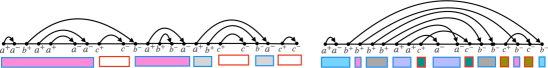
Figure 2: Context and block decomposition for a computation over $\overline{\Gamma}_{2}$ in Figure 1. The blue and red lined rectangles are the two contexts. The color filled rectangles represent blocks, with partner cancelling blocks having the same color filling.

Let $w\in X_{\Gamma}^{*}$ such that $w\equiv_{\Gamma}\varepsilon$ with a reduction $\pi$. We call a decomposition $w=w_{1}\cdots w_{m}$ a block decomposition if it refines the canonical context decomposition and for each $w_{i}$, there is a $w_{j}$ such that $R_{\pi}$ relates every position in $w_{i}$ with a position in $w_{i}$ itself or in $w_{j}$. Here, we do not rule out $i=j$: A block may itself reduce to $\varepsilon$.

Free reductions Block decompositions are closely related to free reductions. Let $w_{1},\dots,w_{m}$ be a sequence of computations in $X_{\Gamma}^{*}$. A free reduction is a finite sequence of applications of the rewriting rules below to consecutive entries of the sequence so that $w_{1},\dots,w_{m}$ gets transformed into the empty sequence.

(FR1) $w_{i},w_{j}\mapsto_{\mathit{free}}\varepsilon$ if $w_{i}w_{j}\equiv_{\Gamma}\varepsilon$

(FR2) $w_{i},w_{j}\mapsto_{\mathit{free}}w_{j},w_{i}$ if $w_{i}Iw_{j}$

(FR3) $w_{i}\mapsto_{\mathit{free}}\hat{w}_{i}$ if $w_{i}\stackrel{{\scriptstyle*}}{{\mapsto_{red}}}\hat{w}_{i}$ using rules R1 and R2

We say that $w_{1},\dots,w_{m}$ is freely reducible if it admits a free reduction to the empty sequence.

As in [20], we have :

Proposition 5.1.

If the decomposition $w=w_{1}\cdots w_{m}$ refines the context decomposition, then it is a block decomposition if and only if the sequence $w_{1},\ldots,w_{m}$ is freely reducible.

The main result of this section is that in a scope-bounded run, there exists a block decomposition with a bounded number of factors in each context.

Theorem 5.2.

Let $w\in X_{\Gamma}^{*}$ with $\mathsf{sc}(w)\leq k$. Then, there exists a block decomposition of $w$ such that each context splits into at most $2k$ blocks.

Let us sketch the proof. The block decomposition is obtained by scanning each context $c$ from left to right. As long as there is another context $c^{\prime}$ such that all symbols either cancel inside $c$ or with a symbol in $c^{\prime}$, we add symbols to the current block. When we encounter a symbol that cancels with a position outside of $c$ and $c^{\prime}$, we start a new block. This clearly yields a block decomposition (see Figure 2 for an example) and with arguments similar to [20], one can show that it results in at most $2k$ blocks per context.

6 Decision procedure

In this section, we present the algorithms for the upper bounds of Theorems 4.1 and 4.3.

Block abstractions The algorithm for bounded context switching in [20] abstracts each block by a non-deterministic automaton. This approach uses polynomial space per block, which would not be a problem for our $\PSPACE$ algorithm. However, for our $\P$ and $\NL$ algorithms, this would require too much space. Therefore, we begin with a new notion of “block abstraction”, which is more space efficient.

Let $w=w_{1}\cdots w_{m}$ be a block decomposition for a run of a valence system $\mathcal{A}$. Then it follows from Proposition 5.1 that there are words $\hat{w}_{1},\ldots,\hat{w}_{m}$ such that $w_{i}\stackrel{{\scriptstyle*}}{{\mapsto_{red}}}\hat{w}_{i}$ for each $i$ such that the sequence $\hat{w}_{1},\ldots,\hat{w}_{m}$ can be reduced to the empty sequence using the rewriting rules FR1 and FR2. For each $i$, we store (i) the states occupied at the beginning and end of $w_{i}$, (ii) its first operation $f\in X_{\Gamma}$ in $w_{i}$, (iii) a non-deterministically chosen operation $o\in X_{\Gamma}$ occurring in $w_{i}$, and (iv) sets $U_{i}^{\mathop{\mathsf{min}}\,}$ and $U_{i}^{\mathop{\mathsf{max}}\,}$, such that every maximal vertex occurring in $w_{i}$ is contained in $U_{i}^{\mathop{\mathsf{max}}\,}$ and every minimal vertex occurring in $\hat{w}_{i}$ is contained in $U_{i}^{\mathop{\mathsf{min}}\,}$. In this case, we will say that the block abstraction “represents” the word $\hat{w}_{i}$. Thus, a block abstration is a tuple $N=(q_{1},q_{2},f,o,U^{\mathop{\mathsf{min}}\,},U^{\mathop{\mathsf{max}}\,})$, where $q_{1},q_{2}$ are states in $\mathcal{A}$, $f,o\in X_{\Gamma}$ are symbols, and $U^{\mathop{\mathsf{min}}\,},U^{\mathop{\mathsf{max}}\,}\subseteq V$ are neighbor antichains. Note that for every set $B\subseteq V$, the sets ${\mathop{\mathsf{min}}\,}B$ and ${\mathop{\mathsf{max}}\,}B$ are neighbor antichains. Formally, we say that $N=(q_{1},q_{2},f,o,U^{\mathop{\mathsf{min}}\,},U^{\mathop{\mathsf{max}}\,})$ represents $\hat{u}\in X_{\Gamma}^{*}$ if there is a word $u\in X_{\Gamma}^{*}$ such that (i) $u\stackrel{{\scriptstyle*}}{{\mapsto_{red}}}\hat{u}$, (ii) $u$ is read on some path from $q_{1}$ to $q_{2}$, (iii) $u$ begins with $f$, (iv) $o$ occurs in $u$, (iv) the set of vertices $B$ occurring in $u$ is a dependent set, (v) we have ${\mathop{\mathsf{max}}\,}B\subseteq U^{\mathop{\mathsf{max}}\,}$, and (vi) ${\mathop{\mathsf{min}}\,}\hat{B}\subseteq U^{\mathop{\mathsf{min}}\,}$, where $\hat{B}$ is the set of vertices occurring in $\hat{u}$. Then, $L(N)$ denotes the set of all words represented by $N$. We say that two block abstractions $N=(q_{1},q_{2},f,o,U^{\mathop{\mathsf{min}}\,},U^{\mathop{\mathsf{max}}\,})$ and $N^{\prime}=(q^{\prime}_{1},q^{\prime}_{2},f^{\prime},o^{\prime},U^{\prime{\mathop{\mathsf{min}}\,}},U^{\prime{\mathop{\mathsf{max}}\,}})$ are dependent if $U^{\mathop{\mathsf{max}}\,}\cup U^{\prime{\mathop{\mathsf{max}}\,}}$ is a dependent set.

Context abstractions Similarly, we will also need to abstract contexts. For this, we need to abstract each of its blocks. In addition, we need to store the whole context’s first symbol ($f$) and some non-deterministically chosen other symbol ($o$). These additional symbols will be used to verify that we correctly guessed the context decomposition of $w$. Thus, a context abstraction is a tuple $\mathcal{C}=(N_{1},\ldots,N_{2k},f,o)$, where $N_{1},\ldots,N_{2k}$ are pairwise dependent block abstractions, and $f$ and $o$ are symbols. We say that a context abstraction $\mathcal{C}=(N_{1},\ldots,N_{2k},f,o)$ is independent with a context abstraction $\mathcal{C^{\prime}}=(N^{\prime}_{1},\ldots,N^{\prime}_{2k},f^{\prime},o^{\prime})$ if (i) $f^{\prime}Io$ and (ii) for some $i\in\{1,\ldots,2k\}$, the block abstraction $N_{i}=(q^{i}_{1},q^{i}_{2},f_{i},o_{i},U_{i}^{\mathop{\mathsf{min}}\,},U_{i}^{\mathop{\mathsf{max}}\,})$ satisfies $o=o_{i}$. Intuitively, this means if we have a word represented by $\mathcal{C^{\prime}}$ and then append a word represented by $\mathcal{C}$, then these words will be the contexts in the canonical context decomposition.

In our algorithms, we will need to check whether a block decomposition admits a free reduction. This means, we need to check whether the words represented by block abstractions can cancel (to apply rule FR1) or commute (to apply FR2). Let us see how to do this. We say that the block abstractions $N=(q_{1},q_{2},f,o,U^{\mathop{\mathsf{min}}\,},U^{\mathop{\mathsf{max}}\,})$ and $N^{\prime}=(q^{\prime}_{1},q^{\prime}_{2},f^{\prime},o^{\prime},U^{\prime{\mathop{\mathsf{min}}\,}},U^{\prime{\mathop{\mathsf{max}}\,}})$ commute if $U^{\mathop{\mathsf{min}}\,}IU^{\prime{\mathop{\mathsf{min}}\,}}$. Note that if $N$ and $N^{\prime}$ commute, then $uIu^{\prime}$ for every $u\in L(N)$ and $u^{\prime}\in L(N^{\prime})$. We need an analogous condition for cancellation. We say that $N$ and $N^{\prime}$ cancel if there are words $u\in L(N)$ and $u^{\prime}\in L(N^{\prime})$ such that $uu^{\prime}\equiv_{\Gamma}\varepsilon$. This allows us to define an analogue of free reductions on block abstractions.

Definition 6.1.

A free reduction on a sequence $N_{1},\ldots,N_{m}$ of block abstractions is a sequence of operations

(FRA1) $N_{i},N_{j}\rightarrow_{\mathit{free}}\varepsilon$, if $N_{i}$ and $N_{j}$ cancel
(FRA2) $N_{i},N_{j}\rightarrow_{\mathit{free}}N_{j},N_{i}$, if $N_{i}$ and $N_{j}$ commute.

Together with Lemma 3.2, the following Lemma allows us to verify the steps in a free reduction on block abstractions.

Lemma 6.2.

Given $\Gamma$, a valence system over $\Gamma$, and block abstractions $N_{1}$ and $N_{2}$, one can decide in $\mathsf{P}$ whether $N_{1}$ and $N_{2}$ cancel. If $\Gamma$ is a clique, this can be decided in $\NL$.

Given block abstractions $N_{1}$ and $N_{2}$, (i) first perform saturation [20], obtaining irreducible blocks. Saturation can be implemented using reachability in a one counter automaton, known to be NL-complete [9], (ii) second, construct a pushdown automaton that is non-empty if and only if the saturated $N_{1}$ and $N_{2}$ cancel. Emptiness of pushdown automata is decidable in $\P$. If $\Gamma$ is a clique, then the pushdown automaton uses only a single stack symbol. Hence, we only need a one-counter automaton, for which emptiness is decidable in $\NL$ [9]. This yields the two upper bounds claimed in Lemma 6.2.

Reduction to a Reachability Graph In all our algorithms, we reduce $\mathsf{BSREACH}$ for a valence system $\mathcal{A}$ over $\Gamma$ to reachability in a finite graph $\mathcal{R}$. For the $\PSPACE$ algorithm, we argue that each node of $\mathcal{R}$ requires polynomially many bits and the edge relation can be decided in $\PSPACE$. For the $\P$ and the $\NL$ algorithm, we argue that $\mathcal{R}$ is polynomial in size. Moreover, for the $\P$ algorithm, we compute $\mathcal{R}$ in polynomial time. For the $\NL$ algorithm, we show that the edge relation of $\mathcal{R}$ can be decided in $\NL$.

The vertices of $\mathcal{R}$ maintain $k$ context abstractions (hence $2k^{2}$ block abstractions) per weak dependence class. Let $d\leq|V|$ be the number of weak dependence classes. The idea behind this choice of vertices is to build up a computation $w$ from left to right, by guessing $k$ context abstractions $\left(\mathcal{C}^{\gamma}_{1},\mathcal{C}^{\gamma}_{2},\cdots,\mathcal{C}^{\gamma}_{k}\right)$ per equivalence class $\gamma$ which forms the “current window” of $w$. The initial vertex consists of $k$ tuples $(\mathcal{E},\dots,\mathcal{E})$ per weak dependence equivalence class, where $\mathcal{E}$ is a placeholder representing a cancelled block or an empty block. An edge is added from a vertex $v_{1}$ to a vertex $v_{2}$ in the graph when the left most context in $v_{1}$ corresponding to an equivalence class $\gamma$ cancels out completely, and $v_{2}$ is obtained by appending a fresh context abstraction $\mathcal{C}_{y}^{\gamma}$ to $v_{1}$. Indeed if $w$ is $k$ scope bounded, then the blocks of the first context abstraction $\mathcal{C}^{\gamma}_{1}$ must cancel out with blocks from the remaining context abstractions $\mathcal{C}^{\gamma}_{2},\cdots,\mathcal{C}^{\gamma}_{k}$ using the free reduction rules discussed above. We can guess an equivalence class $\gamma$ whose context abstraction $\mathcal{C}^{\gamma}_{1}$ cancels out, and extend $w$ by guessing the next context abstraction $\mathcal{C}_{y}^{\gamma}$ in the same equivalence class. An edge between two vertices in $\mathcal{R}$ represents an extension of $w$ where a new context of an appropriate equivalence class is added, after the leftmost context has cancelled out using some free reduction rules.

For a weak dependence class, we refer to the tuple of $k$ contexts of interest as a configuration. Thus, a vertex in $\mathcal{R}$ consists of $d$ configurations. As discussed earlier in section 6, we represent the $2k^{2}$ blocks in each configuration using block abstractions.

Definition 6.3.

Given a weak dependence class $\gamma\in[\leavevmode\nobreak\ ]_{\sim_{W}}$, a configuration of $\gamma$ is a $k$-tuple of the form $s_{\gamma}=(\mathcal{C}^{\gamma}_{1},\mathcal{C}^{\gamma}_{2},\cdots,\mathcal{C}^{\gamma}_{k})$, where each $\mathcal{C}^{\gamma}_{c}$ for $1\leq c\leq k$ is a context abstraction.

As mentioned above, in slight abuse of terminology, in case of cancellation in free reductions, we also allow $\mathcal{E}$ as a placeholder for cancelled contexts.

Intuitively, the configuration tracks the remaining non-cancelled blocks of the last $k$ contexts of this weak dependence class along with their relative positions in their contexts.

Definition 6.4.

A vertex in the graph $\mathcal{R}$ has the form $(s_{\gamma_{1}},\dots,s_{\gamma_{d}}|i,q)$ where (i) $\gamma_{1},\dots,\gamma_{d}$ are the distinct equivalence classes in $[\leavevmode\nobreak\ ]_{\sim_{W}}$, (ii) each $s_{\gamma_{j}}$ is a configuration, (iii) $i\in\{1,\cdots,d\}$ is the current weak dependence class we are on, and (iv) $q$ is the last state occurring in $s_{\gamma_{i}}$.

Here, if $s_{\gamma_{i}}$ consists just of $\mathcal{E}$, then the last condition is satisfied automatically.

Definition 6.5.

For $\gamma\in[\leavevmode\nobreak\ ]_{\sim_{W}}$, a configuration $s^{\prime}_{\gamma}$ is one-step reachable from a configuration $s_{\gamma}=(\mathcal{C}_{1}^{\gamma},\dots,\mathcal{C}_{k}^{\gamma})$ iff there exists some context abstraction $\mathcal{C}$ and a sequence of free reduction operations on the sequence of block abstractions

$$N^{\gamma 1}_{1},\ldots,N^{\gamma 1}_{2k},N^{\gamma 2}_{1},\ldots,N^{\gamma 2}_{2k},\ldots N^{\gamma k}_{1},\ldots,N^{\gamma k}_{2k},N_{1},\ldots,N_{2k}$$

resulting in the new sequence (placing $\mathcal{E}$ in a position if the block was cancelled due to the free reduction rules; otherwise we keep the same block abstraction)

$$N^{\prime\gamma 1}_{1},\ldots,N^{\prime\gamma 1}_{2k},N^{\prime\gamma 2}_{1},\ldots,N^{\prime\gamma 2}_{2k},\ldots N^{\prime\gamma k}_{1},\ldots,N^{\prime\gamma k}_{2k},N^{\prime\gamma(k+1)}_{1},\ldots,N^{\prime\gamma(k+1)}_{2k}$$

such that $N^{\prime\gamma 1}_{\ell}=\mathcal{E}$, for all $\ell\in\{1,\ldots,2k\}$, and $\left({\mathcal{C^{\prime}}^{\gamma}_{2}},\mathcal{C^{\prime}}^{\gamma}_{3},\cdots,\mathcal{C^{\prime}}^{\gamma}_{k},\mathcal{C^{\prime}}^{\gamma}_{k+1}\right)=s^{\prime}_{\gamma}$, where $\mathcal{C^{\prime}}^{\gamma}_{\ell}=(N^{\prime\gamma\ell}_{1},N^{\prime\gamma\ell}_{2},\cdots,N^{\prime\gamma\ell}_{2k},f^{\gamma\ell},o^{\gamma\ell})$ for $\ell\in\{1,\ldots,k+1\}$, and $N_{1},\ldots,N_{2k}$ are the block abstractions in $\mathcal{C}$. In this case, we write $s_{\gamma}\xrightarrow{\mathcal{C}}s^{\prime}_{\gamma}$.

In short, we can go from $s_{\gamma}$ to $s^{\prime}_{\gamma}$ in one step if we can add some context abstraction to $s_{\gamma}$ so that using free reduction steps, we can reach $s^{\prime}_{\gamma}$ along with clearing the oldest context.

We are now ready to define the edge relation of $\mathcal{R}$.

Definition 6.6.

There is an edge in $\mathcal{R}$ from a vertex $v=(s_{\gamma_{1}},\dots,s_{\gamma_{d}}|j,q)$ to a vertex $v^{\prime}$ iff there is some $i\in\{1,\ldots,d\}$ and a configuration $s^{\prime}_{\gamma_{i}}$ such that (i) $s_{\gamma_{i}}\xrightarrow{\mathcal{C^{\prime}}}s^{\prime}_{\gamma_{i}}$ for some context abstraction $\mathcal{C^{\prime}}$ such that $\mathcal{C^{\prime}}$ is independent with the last context abstraction $\mathcal{C}$ of $s_{\gamma_{j}}$ and (ii) $q$ is the first state in $\mathcal{C^{\prime}}$ and (iii) $v^{\prime}=(s_{\gamma_{1}},\dots,s_{\gamma_{i-1}},s^{\prime}_{\gamma_{i}},s_{\gamma_{i+1}},\dots,s_{\gamma_{d}}|i,q^{\prime})$, where $q^{\prime}$ is the last state of $\mathcal{C^{\prime}}$.

Since a context is a maximal dependent sequence, this check suffices to guarantee independence of words represented by $\mathcal{C^{\prime}}$ and $\mathcal{C}$.

As mentioned above, our algorithm reduces scope-bounded reachability to reachability between two nodes in $\mathcal{R}$. Details can be found in the full version.

Complexity We turn to the upper bounds in Theorems 4.1 and 4.3. Asymptotically, a block abstraction requires $\log|Q|+2t\cdot\log|V|$ bits, where $t$ is an upper bound on the size of neighbor antichains. Per context, we store $2k$ block abstractions and two symbols. Let $d$ be the number of weak dependence classes. In a node of $\mathcal{R}$, we store $k$ contexts per weak dependence class, a number in $\{1,\ldots,d\}$, and a state. Hence, asymptotically, we need $M=dk^{2}(\log|Q|+t\cdot\log|V|)+\log d+\log|Q|$ bits per node of $\mathcal{R}$. To simulate the free reduction, we only need a constant multiple of this. We can thus decide reachability in $\mathcal{R}$ in $\PSPACE$.

Proposition 6.7.

$\mathsf{BSREACH}$ is in $\PSPACE$.

We now look at the upper bounds for the first and second cases of Theorem 4.3.

Proposition 6.8.

Let $\mathcal{G}$ be a class of graphs that is closed under strongly induced subgraphs and neighbor antichain bounded. If $\mathcal{G}$ consists of cliques of bounded size, then for each $k\geq 1$, the problem $\mathsf{BSREACH}_{k}(\mathcal{G})$ belongs to $\NL$.

Proof 6.9.

Our assumptions imply that $d\leq|V|$, $t$, and $k$ are bounded. Thus $M$ is at most logarithmic in the input. Moreover, we can simulate free reductions using logarithmic space, because checking whether two block abstractions cancel can be done in $\NL$ by Lemma 6.2.

Proposition 6.10.

Let $\mathcal{G}$ be a class of graphs that is closed under strongly induced subgraphs and neighbor antichain bounded. If the size of cliques in $\mathcal{G}$ is bounded, then for every $k\geq 1$, the problem $\mathsf{BSREACH}_{k}(\mathcal{G})$ belongs to $\P$.

Proof 6.11.

First observe that as in Proposition 6.8, the parameters $d$, $t$, and $k$ are bounded. To see this for $d$, let $\ell$ be an upper bound on the size of cliques in $\mathcal{G}$. Then, every graph $\Gamma$ in $\mathcal{G}$ can have at most $\ell$ weak dependence classes: Otherwise, $\Gamma$ would have a clique with $\ell+1$ nodes as a strongly induced subgraph, and thus $\mathcal{G}$ would contain a clique with $\ell+1$ nodes. Hence, $d$ is bounded and for a node in $\mathcal{R}$, we need only logarithmic space. Moreover, by Lemma 6.2, we can verify a free reduction step in $\P$.

Special Graphs We turn to the $\NL$ and $\P$ upper bounds for Theorem 4.1. In each case, all graphs are anti-cliques. Thus, every run has a single context and $\mathsf{BSREACH}$ reduces to membership for pushdown automata, which is in $\P$. If there is just one vertex, we can even obtain a one-counter automaton, for which emptiness is in $\NL$ [9].

Proposition 6.12.

If $\mathcal{G}$ is the class of anti-cliques, then $\mathsf{BSREACH}(\mathcal{G})$ is in $\P$. Moreover, if $\Gamma$ has only one vertex, then $\mathsf{BSREACH}(\Gamma)$ is in $\NL$.

7 Hardness

In this section, we show the hardness results of Theorems 4.1 and 4.3.

Proposition 7.1.

If $\Gamma$ is not a clique, then $\mathsf{BSREACH}_{k}(\Gamma)$ is $\P$-hard for each $k\geq 1$.

This uses standard techniques. If a valence system uses only the two non-adjacent vertices in $\Gamma$, then scope-bounded reachability is the same as ordinary reachability. If both vertices are looped, then this is the rational subset membership problem for a free group of rank 2, for which $\P$-hardness was observed in [15, Theorem III.4]. If at least one vertex is unlooped, a standard encoding yields a reduction from emptiness of pushdown automata.

Two adjacent vertices and bounded queue automata Our second hardness proof shows $\PSPACE$-hardness in Theorem 4.1.

Proposition 7.2.

If $\Gamma$ has two adjacent nodes, then $\mathsf{BSREACH}(\Gamma)$ is $\PSPACE$-hard.

For the proof of Proposition 7.2, we employ the model of bounded queue automata. A bounded queue automaton (BQA) is a tuple $\mathcal{A}=(Q,n,T,q_{0},q_{f})$, where (i) $Q$ is a finite set of states, (ii) $n\in\mathbb{N}$ is the queue length, given in unary, (iii) $T$ is its set of transitions, (iv) $q_{0}\in Q$ is its initial state, and (iv) $q_{f}\subseteq Q$ is its final state. A configuration of a BQA is a pair $(q,w)\in Q\times\{0,1\}^{n}$. A transition is of the form $(q,x,y,q^{\prime})$, where $q,q^{\prime}\in Q$ and $x,y\in\{0,1\}$. We write $(q,w)\rightarrow(q^{\prime},w^{\prime})$ if there is a transition $(q,x,y,q^{\prime})$ such that (i) $w$ has prefix $x$ and (ii) removing $x$ from the left and appending $y$ on the right yields $w^{\prime}$. The reachability problem for BQA is the following: Given a bounded queue automaton $(Q,n,T,q_{0},q_{f})$, is it true that $(q_{0},0^{n})\xrightarrow{*}(q_{f},0^{n})$? It is straightforward to simulate a linear bounded automaton using a bounded queue automaton and vice-versa, hence reachability for BQA is $\PSPACE$-complete.

General idea and challenge Let us first assume that the nodes $u$ and $v$ in $\Gamma$ are not weakly dependent. The initial approach for Proposition 7.2 is to encode the queue content in the current window of $k=n$ contexts. In each context, we encode a $0$-bit using an occurrence of the letter $u^{+}$ that can only be cancelled with a future $u^{-}$. We call this a $0$-context. Likewise, a $1$-bit is encoded by two occurrences of $u$, which we call a $1$-context. Therefore, we abbreviate $\mathbf{0}=u^{+}$ and $\mathbf{1}=u^{+}u^{+}$. We also have the right inverses $\bar{\mathbf{0}}=u^{-}$ and $\bar{\mathbf{1}}=u^{-}u^{-}$. To start a new context, we multiply $v^{+}v^{-}$ and use the abbreviation $\|=v^{+}v^{-}$. With this encoding, it is easy to check that the oldest context is a $0$-context: Just multiply $\bar{\mathbf{0}}=u^{-}$ and then start a new context using $\|=v^{+}v^{-}$. This can only succeed if the oldest context encodes a $0$: If it had encoded a $1$, there would be another occurrence of $u^{+}$ that can never be cancelled.

However, it is not so easy to check that the oldest context is a $1$-context. One could multiply with $\bar{\mathbf{1}}\|=u^{-}u^{-}v^{+}v^{-}$, but this can succeed even if the oldest context is a $0$-context: Indeed, the first occurrence of $u^{-}$ can cancel with the $u^{+}$ in the oldest context $c$, but the second $u^{-}$ could cancel with $u^{+}$ in a context to the right of $c$.

Solution We overcome this as follows. Instead of one context per bit, we use three contexts. To encode a $0$ in the queue, we use a $0$-context, a $1$-context, and another $1$-context, resulting in the string $011$. To encode a $1$, we do the same with the bit string $100$. Then, we use the above approach to check for $011$ or $100$: Since a successful check for a $0$-context guarantees that there was a $0$-context, checking for $0,1,1$ guarantees that the oldest context is a $0$-context, thus the three oldest contexts must carry $011$. When we check for $1,0,0$, then among the three oldest contexts, at least two are $0$-contexts, hence the three oldest contexts carry $100$.

Let us calculate the required scope bound to implement this idea. Since we only use the operations $u^{+},u^{-},v^{+},v^{-}$, we only have $u$-contexts (consisting of $u^{+},u^{-}$) and $v$-contexts (consisting of $v^{+},v^{-}$). When we read the oldest bit in the queue, we produce three new $u$-contexts (separated by $v$-contexts). Then, we need to write a new bit in the queue, which requires another three $u$-contexts (separated by $v$-contexts). The interaction distance to the oldest $u$-context that is part of the leftmost queue bit is always $k=3(2n-1)$: The oldest bit is encoded using three $u$-contexts. For each further queue entry $i\in\{2,\ldots,n\}$, we have three $u$-contexts that were used to read an even older bit, and then three $u$-contexts that encode the $i$-th bit in the queue. In total, this yields $3(1+2(n-1))=3(2n-1)$ many $u$-contexts.

To initialize the queue, we use $t_{0}=(\mathbf{0}\|\mathbf{1}\|\mathbf{1}\|)(\mathbf{e}\|\mathbf{e}\|\mathbf{e}\|\mathbf{0}\|\mathbf{1}\|\mathbf{1}\|)^{n-1}$. Here, $\mathbf{e}=u^{+}u^{-}$ is a “gap context” that ensures that the leftmost bit has interaction distance exactly $k=3(2n-1)$ from the right end of $t_{0}$. Thus, $t_{0}$ puts $n$ copies of the bit string $011$, plus $n-1$ gap contexts into our window of $k=3(2n-1)$ contexts. To simulate a transition $(p,x,y,p^{\prime})$, we check that $x$ is the bit encoded by the three oldest contexts. Afterwards, we put the new bit $y$ into the queue. Therefore, if $x=0$, define the triple $(x_{1},x_{2},x_{3})=(\bar{\mathbf{0}},\bar{\mathbf{1}},\bar{\mathbf{1}})$; if $x=1$, let $(x_{1},x_{2},x_{3})=(\bar{\mathbf{1}},\bar{\mathbf{0}},\bar{\mathbf{0}})$. Moreover, if $y=0$, then let $(y_{1},y_{2},y_{3})=(\mathbf{0},\mathbf{1},\mathbf{1})$; if $y=1$, then let $(y_{1},y_{2},y_{3})=(\mathbf{1},\mathbf{0},\mathbf{0})$. Then we use the string $t_{x,y}=x_{1}\|x_{2}\|x_{3}\|y_{1}\|y_{2}\|y_{3}\|$. Finally, to check that the encoded queue content consists entirely of $0$’s, we use $t_{f}=(\bar{\mathbf{0}}\|\bar{\mathbf{1}}\|\bar{\mathbf{1}}\|)(\mathbf{e}\|\mathbf{e}\|\mathbf{e}\|\bar{\mathbf{0}}\|\bar{\mathbf{1}}\|\bar{\mathbf{1}}\|)^{n-1}$. With this encoding, it is straightforward to translate a BQA into a valence system over $\Gamma$.

Note that if $u$ and $v$ are weakly dependent, then the same construction works, except that we have to set $k=6(2n-1)$, because now the $v$-contexts $\|=v^{+}v^{-}$ between two $u$-contexts count towards the interaction distance.

Unbounded cliques and bit vector automata We turn to $\PSPACE$-hardness in Theorem 4.3.

Proposition 7.3.

Suppose $\mathcal{G}$ be either the class of unlooped cliques or the class of looped cliques. Then for every $k\geq 1$, the problem $\mathsf{BSREACH}_{k}(\mathcal{G})$ is $\PSPACE$-hard.

Here it is convenient to reduce from bit vector automata, whose configuration consists of a state and a bit vector. In each step, they can read and modify one of the bits. A bit vector automaton (BVA) is a tuple $(Q,n,T,q_{0},q_{f})$, where (i) $Q$ is a finite set of states, (ii) $n$ is the vector length, given in unary, (iii) a set $T$ of transitions, (iv) $q_{0}\in Q$ is its initial state, and (v) $q_{f}\in Q$ is its final state. A transition is of the form $(p,i,x,y,q)$ with $p,q\in Q$, $i\in\{0,\ldots,n\}$, and $x,y\in\{0,1\}$. It checks that $i$-th bit is currently $x$, and sets the $i$-th bit to $y$. Thus, a configuration of a bit vector automaton is a pair $(q,w)\in Q\times\{0,1\}^{n}$. By $\xrightarrow{*}$, we denote the reachability relation. The reachability problem for BVA asks, given a BVA $(Q,n,T,q_{0},q_{f})$, is it true that $(q_{0},0^{n})\xrightarrow{*}(q_{f},0^{n})$? Again, a simulation of linear bounded automata is straightforward and this problem is $\PSPACE$-complete.

Proof 7.4 (Proof of Proposition 7.3).

Let $\mathcal{A}=(Q,n,T,q_{0},q_{f})$ be a BVA. Moreover, depending on whether $\mathcal{G}$ is the class of looped or unlooped cliques, let $\Gamma=(V,I)$ be either a looped or an unlooped clique with $2n$ vertices, so let $V=\{a_{i},b_{i}\mid i\in\{1,\ldots,n\}\}$. Our construction does not depend on whether $\Gamma$ is looped or unlooped and we will show that it is correct in either case. We first illustrate the idea for maintaining a single bit using the vertices $a_{i},b_{i}$. To ease notation, we now write $v$ for $v^{+}$ and $\bar{v}$ for $v^{-}$ when $v\in V$. Consider the string

$$w=(a_{i}^{r_{1}}b_{i}\bar{b}_{i}\bar{a}_{i}^{s_{1}}b_{i}\bar{b}_{i})(a_{i}\bar{a}_{i}b_{i}\bar{b}_{i})^{k}(a_{i}^{r_{2}}b_{i}\bar{b}_{i}\bar{a}_{i}^{s_{2}}b_{i}\bar{b}_{i})\cdots(a_{i}\bar{a}_{i}b_{i}\bar{b}_{i})^{k}(a_{i}^{r_{m}}b_{i}\bar{b}_{i}\bar{a}_{i}^{s_{m}}b_{i}\bar{b}_{i}).$$

Moreover, assume that for each $j=1,\ldots,m$, we have $r_{j},s_{j}\in\{k,3k\}$. We think of $a_{i}^{r_{j}}b_{i}\bar{b}_{i}$ as an operation that stores $0$ if $r_{j}=k$ and stores $1$ if $r_{j}=3k$. We think of $\bar{a}_{i}^{s_{j}}b_{i}\bar{b}_{i}$ as a read operation, where again $s_{j}=k$ stands for 0 and $s_{j}=3k$ stands for $1$. Here, the purpose of $b_{i}\bar{b}_{i}$ is to start a new context (since $\Gamma$ is a clique). Moreover, each factor $(a_{i}\bar{a}_{i}b_{i}\bar{b}_{i})^{k}$ produces $k$ contexts in the weak dependence class of $a_{i}$, where each context contains $a_{i}\bar{a}_{i}$. This means, each factor $(a_{i}\bar{a}_{i}b_{i}\bar{b}_{i})^{k}$ enforces an interaction distance of $k+1$ between $\bar{a}_{i}^{s_{j}}$ and $a_{i}^{r_{j+1}}$, and thus prevents them from canceling with each other.

We claim that $\mathsf{sc}(w)\leq k$ if and only if each read operation reads the bit that was stored before. In other words, we have $\mathsf{sc}(w)\leq k$ if and only if $r_{j}=s_{j}$ for each $j\in\{1,\ldots,m\}$. Moreover, this is true regardless of whether $\Gamma$ is looped or unlooped. For the “if”, note that each $a_{i}^{r_{j}}$ can cancel with $\bar{a}_{i}^{s_{j}}$ and in every other context, every letter ($a_{i}$, $\bar{a}_{i}$, $b_{i}$, $\bar{b}_{i}$) can cancel with its direct neighbor. Conversely, suppose $r_{j}\neq s_{j}$ for some $j$. If $r_{j}=3k$ and $s_{j}=k$, then the context $a_{i}^{r_{j}}=a_{i}^{3k}$ sees only $3k-1$ occurrences of $\bar{a}_{i}$ in contexts at interaction distance $\leq k$: First, the context $\bar{a}_{i}^{s_{i}}=\bar{a}_{i}^{k}$ yields $k$ occurrences. The other $2k-1$ contexts are of the form $a_{i}\bar{a}_{i}$ and each provides one occurrence of $\bar{a}_{i}$. In total, we have $k+2k-1=3k-1$. It is thus impossible to cancel every letter in $a_{i}^{r_{j}}$. The case $r_{j}=k$ and $s_{j}=3k$ is symmetric. This proves our claim. Using this encoding, it is now straightforward to simulate $n$ bits.

Propositions 7.1, 7.2 and 7.3 are the last remaining ingredients for Theorems 4.1 and 4.3: Theorem 4.1 follows from Propositions 6.7, 6.12, 7.1 and 7.2. Moreover, Theorem 4.3 follows from Propositions 6.7, 6.8, 6.10, 7.1 and 7.3.

8 Conclusion

We have introduced a notion of scope-bounded reachability for valence systems over graph monoids. In the special case of graphs that correspond to multi-pushdowns, this notion coincides with the original notion of scope-boundedness introduced by La Torre, Napoli, and Parlato [27]. We have shown that with this notion, scope-bounded reachability is decidable in $\PSPACE$, even if the graph and the scope bound $k$ are part of the input.

In addition, we have studied the complexity of the problem under four types of restrictions: (i) $k$ and the graph are part of the input, and the graph is drawn from some class $\mathcal{G}$ of graphs, (Theorem 4.1), (ii) $k$ is part of the input and the graph is fixed (Corollary 4.2), (iii) $k$ is fixed and the graph is drawn from some class $\mathcal{G}$ of graphs that is neighbor antichain bounded and closed under strongly induced subgraphs (Theorem 4.3) and (iv) $k$ is fixed and the graph is fixed (Corollary 4.4). We have completely determined the complexity landscape in the situations (i)–(iv): In every case, we obtain $\NL$-, $\P$-, or $\PSPACE$-completeness.

These results settle the complexity of scope-bounded reachability for most types of infinite-state systems that fit in the framework of valence systems and have been considered in the literature.

Open Problem: Dropping neighbor antichain boundedness

However, we leave open what complexities can arise if in case (iii) above, we drop the assumption of neighbor antichain boundedness. In other words: $k$ is fixed and the graph comes from a class $\mathcal{G}$ that is closed under strongly induced subgraphs. For all we know, it is possible that there are classes $\mathcal{G}$ for which the problem is neither $\NL$-, nor $\P$-, nor $\PSPACE$-complete.

For example, for each $n\geq 0$, consider the bipartite graph $B_{n}$ with nodes $\{u_{i},v_{i}\mid i\in\{1,\ldots,n\}\}$, where $\{u_{i},v_{j}\}$ is an edge if and only if $i\neq j$. Moreover, let $\mathcal{G}$ be the class of graphs containing $B_{n}$ for every $n\in\mathbb{N}$ and all strongly induced subgraphs. Observe that the cliques in $\mathcal{G}$ have size at most 2: $B_{n}$ is bipartite and thus every clique in $B_{n}$ has size at most $2$. In particular, if a clique is a strongly induced subgraph of $B_{n}$, then it can be of size at most $2$. Moreover, the graphs $B_{n}$ have neighbor antichains of unbounded size: The set $\{u_{1},\ldots,u_{n}\}$ is a neighbor antichain in $B_{n}$.

We currently do not know the exact complexity of $\mathsf{BSREACH}_{k}(\mathcal{G})$. By Theorem 4.3, the problem is $\P$-hard and in $\PSPACE$. Intuitively, our $\P$ upper bound does not apply because in each node of $\mathcal{R}$, one would have to remember $n$ bits in order to keep enough information about commutation of blocks: For a subset $S\subseteq\{1,\ldots,n\}$, let $u_{S}$ be the product of all $u_{1}^{+},\ldots,u_{n}^{+}$, where we only include $u_{i}^{+}$ if $i\in S$. Then $u_{S}v_{j}^{+}\equiv v_{j}^{+}u_{S}$ if and only if $j\notin S$.

Appendix A Additional material for Section 3

Proof of Lemma 3.2

Proof A.1.

Assume $UIU^{\prime}$. That is, for all $u\in U$, $u^{\prime}\in U^{\prime}$, $uIu^{\prime}$. Assume that $\neg[({\mathop{\mathsf{min}}\,}U)I({\mathop{\mathsf{min}}\,}U^{\prime})]$. Then there is some $v\in{\mathop{\mathsf{min}}\,}(U)\subseteq U,v^{\prime}\in\min(U^{\prime})\subseteq U^{\prime}$ such that $v,v^{\prime}$ are dependent. This contradicts $UIU^{\prime}$. Likewise, if $({\mathop{\mathsf{min}}\,}U)I({\mathop{\mathsf{min}}\,}U^{\prime})$ then $uIu^{\prime}$ for all $u\in{\mathop{\mathsf{min}}\,}(U),u^{\prime}\in{\mathop{\mathsf{min}}\,}(U^{\prime})$. Assume $\neg(UIU^{\prime})$. Consider $u\prec v,v\in U$ and $u^{\prime}\prec v^{\prime},v^{\prime}\in U^{\prime}$ such that $\neg(vIv^{\prime})$. The last condition is possible by assumption that $\neg(UIU^{\prime})$. Then we have $N(u)\subset N(v),N(u^{\prime})\subset N(v^{\prime})$ but $\neg(vIv^{\prime})$. Since $uIu^{\prime}$ and $u\prec v,u^{\prime}\prec v^{\prime}$, we have $v^{\prime}\in N(u)$ and $v\in N(u^{\prime})$. Hence, $v^{\prime}\in N(v),v\in N(v^{\prime})$ giving $vIv^{\prime}$. Since this is true for any $u\prec v,u^{\prime}\prec v^{\prime}$, we obtain $vIv^{\prime}$ for all such $v,v^{\prime}$, contradicting $\neg(UIU^{\prime})$. Hence we have $UIU^{\prime}$.

Appendix B Additional material for Section 4

Counterexample with neighbor antichain boundedness Consider the bipartite graph $B_{n}$ with nodes $\{u_{i},v_{i}\mid i\in\{1,\ldots,n\}\}$, where $\{u_{i},v_{j}\}$ is an edge if and only if $i\neq j$. Moreover, let $\mathcal{G}$ be the class of graphs containing $B_{n}$ for every $n\in\mathbb{N}$ and all strongly induced subgraphs. Observe that the cliques in $\mathcal{G}$ have size at most 2: $B_{n}$ is bipartite and thus contains cliques of size at most $2$. In particular, if a clique is a strongly induced subgraph of $B_{n}$, then it can be of size at most $2$. Moreover, the graphs $B_{n}$ have neighbor antichains of unbounded size: The set $\{u_{1},\ldots,u_{n}\}$ is a neighbor antichain in $B_{n}$.

We currently do not know the exact complexity of $\mathsf{BSREACH}_{k}(\mathcal{G})$. By Theorem 4.3, the problem is $\P$-hard and in $\PSPACE$. Intuitively, our $\P$ upper bound does not apply because in each node of $\mathcal{R}$, one would have to remember $n$ bits in order to keep enough information about commutation of blocks: For a subset $S\subseteq\{1,\ldots,n\}$, let $u_{S}$ be the product of all $u_{1}^{+},\ldots,u_{n}^{+}$, where we only include $u_{i}^{+}$ if $i\in S$. Then we have $u_{S}v_{j}^{-}\equiv v_{j}^{+}u_{S}$ if and only if $j\notin S$.

Appendix C Additional material for Section 5

In this section, we provide detailed proofs for Proposition 5.1 and Theorem 5.2.

Block decompositions and free reductions

We begin with Proposition 5.1. For this (and for Theorem 5.2), we need a simple lemma that allows us to conclude independencies from relations $R_{\pi}$.

Lemma C.1.

Suppose $\pi$ is a reduction for $w\stackrel{{\scriptstyle*}}{{\mapsto_{red}}}\varepsilon$. If $i,j,k,\ell$ are positions in $w$ such that $iR_{\pi}j$ and $kR_{\pi}\ell$ with $i<k<j<\ell$, then $w[k]Iw[j]$.

Proof C.2.

Towards a contradiction, suppose that $w[k]$ and $w[\ell]$ are dependent. Then for every word $w^{\prime}$ obtained during the reduction $\pi$, there are positions $i^{\prime}<k^{\prime}<j^{\prime}<\ell^{\prime}$ with $w^{\prime}[i^{\prime}]=w[i]$, $w^{\prime}[k^{\prime}]=w[k]$, $w^{\prime}[j^{\prime}]=w[j]$, and $w^{\prime}[\ell^{\prime}]=w[\ell]$. This follows directly from the definition of reductions by induction on the number of reduction steps: In this situation, we can never move any of the letters $w[i],w[k],w[j],w[\ell]$ past each other and hence we can never cancel any of them as prescribed in $R_{\pi}$. Thus, every word produced during $\pi$ has at least length $4$, in contradiction to the fact that $\pi$ produces $\varepsilon$.

With Lemma C.1, we can now prove: See 5.1

Proof C.3.

Note that the “if” direction is easy to see: If the sequence $w_{1},\ldots,w_{m}$ is freely reducible, then there clearly exists a reduction $\pi$ so that $w_{1},\ldots,w_{m}$ is a block decomposition with respect to $\pi$: We just take the reduction that cancels as the free reduction dictates.

For the converse, suppose there is a reduction $\pi$ of $w_{1}\cdots w_{m}$ such that $w_{1},\ldots,w_{m}$ is a block decomposition with respect to $\pi$. Then for each $w_{i}$, there is a block $w_{j}$ such that every position in $w_{i}$ cancels either with a letter in $w_{i}$ or with a letter in $w_{j}$. In the first step, we consider all those position pairs in $w_{i}$ that are canceled with each other by $\pi$ and cancel them using the rule F3 to obtain a word $\hat{w}_{i}$. Now for the sequence $\hat{w}_{1},\ldots,\hat{w}_{m}$, we have: (i) every $\hat{w}_{i}$ is dependent and (ii) for each $\hat{w}_{i}$, there is a word $\hat{w}_{j}$ such that every position in $\hat{w}_{i}$ cancels with a position in $\hat{w}_{j}$ (and vice versa). A sequence of words for which a reduction with properties (i) and (ii) exists will be called block-like.

We now prove by induction on $m$ that for every block-like sequence $\hat{w}_{1},\ldots,\hat{w}_{m}$, there exists a free reduction (using only rules F1 and F2). For $m=0$, this is trivial, so assume $m>0$. The property (ii) allows us to define a binary relation $\hat{R}$ on $\{1,\ldots,m\}$: We have $i\hat{R}j$ if all the letters in $\hat{w}_{i}$ are $R_{\pi}$-related to letters in $\hat{w}_{j}$. We now call a pair $(i,j)\in\hat{R}$ with $i<j$ minimal if there is no other pair $(i^{\prime},j^{\prime})\in\hat{R}$ with $i^{\prime}<j^{\prime}$ such that $i<i^{\prime}<j^{\prime}<j$.

Clearly, there must be some minimal pair $(i,j)\in\hat{R}$. Now for every $\hat{w}_{k}$ with $i<k<j$, the index $\ell$ with $(k,\ell)\in\hat{R}$ must either satisfy $\ell<i$ or $j<\ell$: Any other arrangement would contradict minimality of $(i,j)$. By Lemma C.1, this implies that all the letters in $\hat{w}_{k}$ are independent with the letters in $\hat{w}_{i}$ and $\hat{w}_{j}$. Therefore, we can apply the following sequence of rules:

1. For every $\hat{w}_{k}$ with $i<k<j$: Move $\hat{w}_{k}$ past $\hat{w}_{j}$ using FR2. We do this starting with the rightmost such $\hat{w}_{k}$. We arrive at the sequence

   $$\hat{w}_{1},\ldots,\hat{w}_{i},\hat{w}_{j},\hat{w}_{i+1},\ldots,\hat{w}_{j-1},\hat{w}_{j+1},\ldots,\hat{w}_{m}.$$

2. We can now apply FR1 to eliminate $\hat{w}_{i},\hat{w}_{j}$. We thus have the sequence

   $$\hat{w}_{1},\ldots,\hat{w}_{i+1},\ldots,\hat{w}_{j-1},\hat{w}_{j+1},\ldots,\hat{w}_{m},$$ (1)

   which differs from $\hat{w}_{1},\ldots,\hat{w}_{m}$ only in the removal of $\hat{w}_{i}$ and $\hat{w}_{j}$.

Now the new sequence (1) is still block-like: The reduction $\pi$ that witnesses block-likeness of $\hat{w}_{1},\ldots,\hat{w}_{m}$ can clearly be turned into one for (1), because the latter is just missing a pair of words that were related by $R_{\pi}$. Thus, by induction, there is a free reduction for (1) and hence also for $\hat{w}_{1},\ldots,\hat{w}_{m}$.

The number of blocks per context

We now prove Theorem 5.2: See 5.2 For the proof of Theorem 5.2, given a word $w$ with a decomposition $w=w_{1}\cdots w_{n}$ into contexts, we associate with any reduction $\pi\colon w\stackrel{{\scriptstyle*}}{{\mapsto_{red}}}\varepsilon$ a refining decomposition. This is the decomposition induced by $\pi$, which is defined as follows.

Consider a computation $w\in\mathcal{O}^{+}$ (that is, $|w|>0$) and a decomposition $w=w_{1}\cdots w_{n}$ into contexts. Let $\pi\colon w\stackrel{{\scriptstyle*}}{{\mapsto_{red}}}\varepsilon$ be a reduction that transforms $w$ into $\varepsilon$.

The decomposition of $w$ induced by $\pi$ is obtained as follows. Parse each context from left to right. Suppose we have a context $w_{i}=w_{i}[1]w_{i}[2]\dots w_{i}[m]$. Each factor in our new decomposition begins at the leftmost position of a context. If the symbol $w_{i}[k]$ at position $k$ cancels with a symbol $w_{j}[\ell]$ (that is, $w_{i}[k]R_{\pi}w_{j}[\ell]$) in some context $w_{j}$ with $j\neq i$ and no other position in the current factor has canceled with a symbol in context $w_{j}$, then we start a new factor from position $w_{i}[k]$. Otherwise, we include $w_{i}[k]$ in the current factor.

Figure 2 illustrates (i) the decomposition of a computation over the graph $\overline{\Gamma}_{2}$ into contexts and (ii) the decomposition induced by $\pi$.

Note that this induced decomposition can be defined for any $w\in X_{\Gamma}^{*}$ with $w\stackrel{{\scriptstyle*}}{{\mapsto_{red}}}\varepsilon$. However, in general, it does not guarantee that the number of factors in a context would be bounded. For example, if we have two adjacent vertices $a,b$, then for every $m\geq 0$, the word $(a^{+}b^{+}b^{-})^{m}(a^{-})^{m}$ decomposes into $m+1$ contexts: $m$ times the context $a^{+}b^{+}b^{-}$ and once the context $(a^{-})^{m}$. However, the last context decomposes into $m$ factors of the form $a^{-}$.

Therefore, for Theorem 5.2, we need to establish two facts, under the assumption that $\pi$ is a reduction witnessing $k$-scope boundedness of $w$: (i) the decomposition induced by $\pi$ is a block decomposition and (ii) this block decomposition splits each context into at most $2k$ blocks. Compared to the block decomposition given in [20], the main difference here is that the number of context switches is unbounded, whereas [20] considered computations with bounded number of context switches.

Lemma C.4.

Let $w=w_{1}\cdots w_{n}$ be a context decomposition and let $\pi\colon w\stackrel{{\scriptstyle*}}{{\mapsto_{red}}}\varepsilon$ be a greedy reduction. Then the decomposition of $w$ induced by $\pi$ has the following property: For any two contexts $w_{i}$ and $w_{j}$, there is at most one factor in $w_{i}$ that is $R_{\pi}$-related to a factor of $w_{j}$.

Proof C.5.

If every position in $w_{i}$ cancels with a position in $w_{i}$, then $w_{i}$ has only one factor, so this case is trivial. If however, there is a position in $w_{i}$ that cancels with another context, then for each factor $f$ in $w_{i}$ from our decomposition, there is a uniquely determined context $w_{j}$, $j\neq i$, such that every position in $f$ cancels either with a position in $w_{i}$ or with a position in $w_{j}$. In this situation, we simply say that $f$ cancels with $w_{j}$.

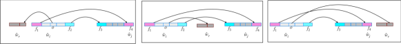
Figure 3: Possible cases for matching in Lemma C.4

We consider for each context $w_{i}$ the word $\hat{w}_{i}$ obtained from $w_{i}$ by removing all positions that cancel with a position in $w_{i}$ itself. Since $\pi$ is greedy, we know that $\hat{w}_{i}$ is irreducible. Moreover, the decomposition $\hat{w}_{1}\cdots\hat{w}_{n}$ is a decomposition into contexts.

Now $\pi$ yields a reduction $\hat{\pi}$ on the decomposition $\hat{w}_{1},\ldots,\hat{w}_{n}$. If we can show our claim for $\hat{w}_{1},\ldots,\hat{w}_{n}$ instead of $w_{1},\ldots,w_{n}$, then this implies the lemma: If there are two distinct factors in $w_{i}$ that both cancel with $w_{j}$, then this yields the same situation in $\hat{w}_{i}$ and $\hat{w}_{j}$.

Toward a contradiction, suppose there were two distinct factors $f_{1}$ and $f_{2}$ in $\hat{w}_{i}$ that both cancel with $\hat{w}_{j}$, but there is a factor in between them.

We begin with some terminology. Consider a position with letter $o$ between $f_{1}$ and $f_{2}$. By assumption, it cancels with some context $\hat{w}_{r}$, $r\neq j$. See Figure 3. If $i<r<j$, then we call this position an inner position (because it cancels with a context between $\hat{w}_{i}$ and $\hat{w}_{j}$). In Figure 3, this is the case shown in the middle. If $r<i$ or $j<r$, then we call this position an outer position. In Figure 3, these are the cases on the left and on the right.

According to Lemma C.1, every inner position must commute with every letter in $f_{2}$. Likewise, every outer position must commute with every letter in $f_{1}$. However, commutation between two positions inside a context is only possible if both letters belong to the same vertex $v$ and one letter is $v^{+}$ and the other is $v^{-}$. Therefore, the position immediately to the right of $f_{1}$ must be an inner position: Otherwise, $\hat{w}_{i}$ would not be irreducible. Likewise, the position immediately to the left of $f_{2}$ must be an outer position. However, that means that somewhere between $f_{1}$ and $f_{2}$, there must be an inner position directly to the left of an outer position. Then, however, Lemma C.1 implies that these two neighboring positions must commute, which again means that they can cancel directly. This is in contradiction to irreducibility of $\hat{w}_{i}$.

Lemma C.6.

Let $w=w_{1}\cdots w_{n}$ be a context decomposition and let $\pi\colon w\stackrel{{\scriptstyle*}}{{\mapsto_{red}}}\varepsilon$ be a reduction. Then the decomposition induced by $\pi$ is a block decomposition.

Proof C.7.

Suppose $\sc(w)\leq k$ and let $\pi\colon w\stackrel{{\scriptstyle*}}{{\mapsto_{red}}}\varepsilon$ be a reduction that witnesses $\sc(w)\leq k$. We first show that the decomposition induced by $\pi$ is indeed a block decomposition. Towards a contradiction, suppose there is a factor $f$ in a context $w_{i}$ such that there exist distinct factors $g$ and $h$ in contexts $w_{j}$ and $w_{k}$, respectively, such that $i\notin\{j,k\}$ and (a) some position in $f$ cancels with a position in $g$ and (b) some position in $f$ cancels with a position in $h$. Then by definition of the induced decomposition, we must have $j=k$, because otherwise we would have started a new factor mid-way in $f$. But this implies that $w_{j}$ has two distinct factors ($g$ and $h$) that each cancel with some position in $w_{i}$, which contradicts Lemma C.4.

Because of Lemma C.6, from now on, we also speak of the block decomposition induced by $\pi$.

We are now ready to prove Theorem 5.2.

Proof C.8 (Proof of Theorem 5.2).

Suppose $\sc(w)\leq k$, let $w=w_{1}\cdots w_{n}$ be decomposition into contexts, and let $\pi\colon w\stackrel{{\scriptstyle*}}{{\mapsto_{red}}}\varepsilon$ be a reduction witnessing $\sc(w)\leq k$. We show that the block decomposition induced by $\pi$ splits each context into at most $2k$ blocks.

Consider a context $w_{i}$. Let $\{b_{1},\ldots,b_{r}\}$ the set of blocks in $w_{i}$. If each position in $w_{i}$ cancels with a position in $w_{i}$, then $w_{i}$ consists of a single block. Thus, we assume that at least one position in $w_{i}$ cancels with a position in some other context. In that case, for each block $b_{\ell}$ in $w_{i}$, there is a unique context $w_{f(\ell)}$ such that every position in $b_{\ell}$ cancels with some position in $w_{i}$ or in $w_{f(\ell)}$. By Lemma C.4, we know that the function $f\colon\{1,\ldots,\ell\}\to\{1,\ldots,n\}$ is injective. Moreover, since $\pi$ is a witness for $k$-scope boundedness, we know that each context $w_{f(\ell)}$ has interaction distance at most $k$ from $w_{i}$. Moreover, $w_{f(\ell)}$ must belong to the same weak dependence class as $w_{i}$. Since there are at most $2k$ blocks at interaction distance $k$ in the same weak dependence class as $w_{i}$, we know that the image $\{f(1),\ldots,f(r)\}$ has at most $2k$ elements. Since $f$ is injective, this implies $r\leq 2k$.

Appendix D Additional material for Section 6

Algorithm 1 $\mathsf{BSREACH}(\Gamma,k)$ : $k$-scope bound reachability for a Valence System

1:Valence System $\mathcal{A}$ over a graph monoid $\mathbb{M}\Gamma$, scope bound $k$.

2:ACCEPT if there a $k$ scope bounded computation $w\in X^{*}_{\Gamma}$, else REJECT.

3:$q\leftarrow q_{init}$

4:$o\leftarrow\phi$

5:$class\leftarrow\phi$

6:for $x\in\{1,\cdots,d\}$, where $d=|[\leavevmode\nobreak\ ]_{\sim_{W}}|$ do

7:     $s_{\gamma_{x}}\leftarrow s_{init}=\left((\mathcal{C}_{1},\varepsilon,\varepsilon),(\mathcal{C}_{2},\varepsilon,\varepsilon),\cdots,(\mathcal{C}_{k},\varepsilon,\varepsilon)\right)$, where $\mathcal{C}_{c}=(\mathcal{E},\mathcal{E},\cdots,\mathcal{E})$

8:end for

9:/* Initialize the configuration */

10:while True do

11:     Guess an equivalence class $x\in\{1,\cdots,d\}$, where $d=|[\leavevmode\nobreak\ ]_{\sim_{W}}|$

12:     $\forall i\in\{1,\cdots,2k\}$ $q^{c}_{i}\leftarrow$ Guess end state for each block abstraction $i$

13:     $\forall i\in\{1,\cdots,2k\}$ Guess ${\mathop{\mathsf{min}}\,}(B_{i}),{\mathop{\mathsf{max}}\,}(B_{i})$ such that

14:     $\leavevmode\nobreak\ \leavevmode\nobreak\ \leavevmode\nobreak\ \leavevmode\nobreak\ \leavevmode\nobreak\ \forall i,j$, ${\mathop{\mathsf{max}}\,}(B_{i})$ and ${\mathop{\mathsf{max}}\,}(B_{j})$ are dependent /* Symbols of blocks $B_{1},\dots,B_{2k}$ mutually dependent */

15:     $\forall i\in\{1,\cdots,2k\}$ Guess $f^{c}_{i}\in V$, the start symbol for each block

16:     if $\neg(f^{c}_{1}\leavevmode\nobreak\ I\leavevmode\nobreak\ o)$ then REJECT

17:     end if

18:     $\forall i\in\{1,\cdots,2k\}$ Guess $o^{c}_{i}\in V$, a symbol that necessarily appears in the block

19:     Guess $o_{c}\in\{o^{c}_{1},\cdots,o^{c}_{2k}\}$ which appears in context $\mathcal{C}_{c}$ /* $o_{c}$ is used to check independence with the first symbol of next context */

20:     Thus, form the next context $\mathcal{C}_{c}=(N^{c}_{1},\cdots,N^{c}_{2k},f_{c},o_{c})$ for $\gamma_{x}$ where $q^{c}_{0}\leftarrow q$ /* start from the last state of previous context */ $f_{c}=f^{c}_{1}$ and $N^{c}_{i}=(q^{c}_{i-1},q^{c}_{i},f^{c}_{i},o^{c}_{i},{\mathop{\mathsf{min}}\,}(B_{i}),{\mathop{\mathsf{max}}\,}(B_{i}))$ $\forall i\in\{1,\cdots,2k\}$

21:     Guess a sequence of free reduction operations $\rightsquigarrow_{red}$ (possibly 0 operations),

22:     to eliminate the leftmost context /* This converts $N^{1}_{1},\cdots,N^{1}_{2k},N^{2}_{1},\cdots,N^{2}_{2k},\cdots N^{k}_{1},\cdots,N^{k}_{2k},N^{c}_{1},\cdots,N^{c}_{2k}$ to $N^{\prime 1}_{1},\cdots,N^{\prime 1}_{2k},N^{\prime 2}_{1},\cdots,N^{\prime 2}_{2k},\cdots N^{\prime k}_{1},\cdots,N^{\prime k}_{2k},N^{\prime c}_{1},\cdots,N^{\prime c}_{2k}$ */

23:     if $\exists i\in\{1,\cdots,2k\}\leavevmode\nobreak\ N^{\prime 1}_{i}\neq\mathcal{E}$ then REJECT

24:     end if

25:     $q\leftarrow q^{c}_{2k}$ /* Store last state of the context in $q$ */

26:     $o\leftarrow o_{c}$ /* Store some seen symbol from this context in $o$ */

27:     $class\leftarrow x$

28:     $s_{\gamma_{x}}\leftarrow((\mathcal{C}^{\prime}_{2},f_{2},o_{2})\cdots,(\mathcal{C}^{\prime}_{k},f_{k},o_{k}),(\mathcal{C}^{\prime}_{c},f_{c},o_{c}))$

29:     if $\forall\gamma\in[\leavevmode\nobreak\ ]_{\sim_{W}}\ \forall c\in\{1,\cdots,k\}\ \forall i\in\{1,\cdots,2k\}\ N^{c}_{i}=\mathcal{E}$ and $q=q_{fin}$ then

30:         ACCEPT

31:     end if

32:end while

D.1 Proof of Lemma 6.2

Given a context abstraction $\mathcal{C}=(N_{bl}^{1},\dots,N_{bl}^{2k},f,o)$ where each $N_{bl}^{i}$ has the form
$(q_{0}^{i},q_{1}^{i},f_{bl},o_{bl},U_{i}^{\mathop{\mathsf{min}}\,},U_{i}^{\mathop{\mathsf{max}}\,})$, one can check whether for any pair of block abstractions $N_{bl}^{i},N_{bl}^{j}$, they are over mutually dependent symbols. To do this, it suffices to check if $U_{i}^{\mathop{\mathsf{max}}\,}$ is dependent with $U_{j}^{\mathop{\mathsf{max}}\,}$. That is, each $u\in U_{i}^{\mathop{\mathsf{max}}\,}$ is dependent with each $u^{\prime}\in U_{j}^{\mathop{\mathsf{max}}\,}$.

Lemma D.1.

(Dependence check between block abstractions) Two block abstractions $N_{bl}^{i},N_{bl}^{j}$ are over mutually dependent symbols iff $U_{i}^{\mathop{\mathsf{max}}\,}$ is dependent with $U_{j}^{\mathop{\mathsf{max}}\,}$.

Proof D.2.

Assume that $N_{bl}^{i},N_{bl}^{j}$ are over mutually dependent symbols. Then clearly, $U_{i}^{\mathop{\mathsf{max}}\,}$ is dependent with $U_{j}^{\mathop{\mathsf{max}}\,}$. Conversely, assume that $U_{i}^{\mathop{\mathsf{max}}\,}$ is dependent with $U_{j}^{\mathop{\mathsf{max}}\,}$. Consider $v_{i}\in U_{i}^{\mathop{\mathsf{max}}\,}$, $w_{i}\in B_{i}$ such that $w_{i}<v_{i}$, and likewise $v_{j}\in U_{j}^{\mathop{\mathsf{max}}\,}$ and $w_{j}\in B_{j}$, with $w_{j}<v_{j}$. Assume $w_{i}Iw_{j}$. Then $w_{i}\in N(v_{j}),w_{j}\in N(v_{i})$ resulting in $v_{i}\in N(v_{j}),v_{j}\in N(v_{i})$. This contradicts the mutual dependence of $U_{i}^{\mathop{\mathsf{max}}\,}$ and $U_{j}^{\mathop{\mathsf{max}}\,}$.

Checking a free reduction between block abstractions

Check if two blocks commute. With the representation of block abstractions, to check if two block abstractions $N_{u},N_{v}$ commute, it is enough to check if $U_{u}^{\mathop{\mathsf{min}}\,}IU_{v}^{\mathop{\mathsf{min}}\,}$ (Lemma 3.2).

Check if two blocks cancel. We now discuss how to use block abstractions to check if two blocks $N_{u},N_{v}$ cancel with each other. Given the block abstractions $N_{u}=(q_{1},q_{2},f_{u},o_{u},U_{u}^{\mathop{\mathsf{min}}\,},U_{u}^{\mathop{\mathsf{max}}\,})$ and $N_{v}$=$(q_{3},q_{4},f_{v},o_{v},U_{v}^{\mathop{\mathsf{min}}\,},U_{v}^{\mathop{\mathsf{max}}\,})$, we first compute

$$B_{i} =\{x\in V\mid\exists y\in U_{i}^{\mathop{\mathsf{max}}\,}\colon x\preceq y\}$$

$$\hat{B}_{i} =\{x\in B_{i}\mid\exists y\in U_{i}^{\mathop{\mathsf{min}}\,}\colon y\preceq x\}$$

for $i\in\{u,v\}$. and the corresponding alphabets

$$X_{i} =\{o^{+},o^{-}\mid o\in B_{i}\}$$

$$\hat{X}_{i} =\{o^{+},o^{-}\mid o\in\hat{B}_{i}\}$$

for $i\in\{u,v\}$.

Then, by definition of cancellation, we have to check whether there are words $w_{u},\hat{w}_{u},w_{v},\hat{w}_{v}$, such that

1. $w_{u}$ is read one some path from $q_{1}$ to $q_{2}$

2. $w_{v}$ is read one some path from $q_{3}$ to $q_{4}$

3. $w_{i}\in X_{i}^{*}$, $\hat{w}_{i}\in\hat{X}_{i}^{*}$ for $i\in\{u,v\}$,

4. $w_{i}\stackrel{{\scriptstyle*}}{{\mapsto_{red}}}\hat{w}_{i}$ using rules R1 and R2, for $i\in\{u,v\}$

5. $\hat{w}_{u}\hat{w}_{v}\equiv_{\Gamma}\varepsilon$.

6. $o_{i}$ occurs in $w_{i}$, for $i\in\{u,v\}$

7. $w_{i}$ begins with $f_{i}$, for $i\in\{u,v\}$

Note that since $\hat{B}_{i}\subseteq B_{i}$, if such words exist, then they exist such that $\hat{w}_{u}$ and $\hat{w}_{v}$ are irreducible. In that case, we must have $\hat{w}_{u},\hat{w}_{v}\in(\hat{X}_{u}\cap\hat{X}_{v})^{*}$.

We now construct a PDA $\mathcal{P}_{uv}$ for the language of all words $w_{u}\#w_{v}$ such that words $\hat{w}_{u}$ and $\hat{w}_{v}$ exist so that conditions 1, 2, 3, 4 and 5 are satisfied. This proves that we can decide cancellation in polynomial time: By intersecting with the regular language

$$\{w_{u}\#w_{v}\mid\text{$o_{i}$ occurs in $w_{i}$, and $w_{i}$ begins with $f_{i}$, for $i\in\{u,v\}$}\},$$

we obtain a PDA that accepts a non-empty set if and only if the two block abstractions cancel.

The PDA $\mathcal{P}_{uv}$ is constructed as follows. Intuitively, we first read the word $w_{u}$ and on the stack, we leave the word $\hat{w}_{v}$. To this end, the stack alphabet contains $\hat{X}_{u}\cap\hat{X}_{u}$ and also separate symbols $\{(x,i)\mid x\in X_{i}\setminus(\hat{X}_{u}\cap\hat{X}_{v})\}$ for $i\in\{u,v\}$. Here, the letters $(x,i)$ are used to simulate internal cancellations in the word $w_{i}$, $i\in\{u,v\}$. Note that we have to make sure that $\hat{w}_{i}$ does not contain any letters from $X_{i}\setminus\hat{X}_{i}$. Therefore, while reading $w_{v}$, our PDA cannot pop letters $(x,u)$, so that it is guaranteed that the word $\hat{w}_{u}$ contains only letters in $\hat{X}_{u}$. Then, after reading $\#$, the automaton reads $w_{v}$ and and makes sure that $\hat{w}_{v}$ cancels with the stack content that existed when it read $\#$.

Its stack alphabet is $\Delta=(\hat{X}_{u}\cap\hat{X}_{v})\cup\{(x,i)\mid x\in X_{i}\setminus(\hat{X}_{u}\cap\hat{X}_{v}),\leavevmode\nobreak\ i\in\{u,v\}\}$. Its set of states is $Q\times\{u,v\}$, where the states $(q,u)$ are used to read $w_{u}$ and the states $(q,v)$ are used to read $w_{v}$. We have the following transitions:

• For every $x\in\hat{B}_{u}\cap\hat{B}_{v}$ and $i\in\{u,v\}$:

  • For every transition $p\xrightarrow{x^{+}}q$, we add a transition from $(p,i)$ to $(q,i)$ that pushes $x^{+}$ and reads $x^{+}$.

  • For every transition $p\xrightarrow{x^{-}}q$, we add a transition from $(p,i)$ to $(q,i)$ that pops $x^{+}$ and reads $x^{-}$.

  • If $xIx$, then for every transition $p\xrightarrow{x^{-}}q$, we add a transition from $(p,i)$ to $(q,i)$ that pushes $x^{-}$ and reads $x^{-}$.

  • If $xIx$, then for every transition $p\xrightarrow{x^{+}}q$, we add a transition from $(p,i)$ to $(q,i)$ that pops $x^{-}$ and reads $x^{+}$.

• For every $x\in B_{i}\setminus(\hat{B}_{u}\cap\hat{B}_{v})$ and $i\in\{u,v\}$:

  • For every transition $p\xrightarrow{x^{+}}q$, we add a transition from $(p,i)$ to $(q,i)$ that pushes $(x^{+},i)$ and reads $x^{+}$.

  • For every transition $p\xrightarrow{x^{-}}q$, we add a transition from $(p,i)$ to $(q,i)$ that pops $(x^{+},i)$ and reads $x^{-}$.

  • If $xIx$, then for every transition $p\xrightarrow{x^{-}}q$, we add a transition from $(p,i)$ to $(q,i)$ that pushes $(x^{-},i)$ and reads $x^{-}$.

  • If $xIx$, then for every transition $p\xrightarrow{x^{+}}q$, we add a transition from $p$ to $q$ that pops $(x^{-},i)$ and reads $x^{+}$.

• We add a transition from $(q_{2},u)$ to $(q_{3},v)$, reading $\#$.

Finally, the initial state of our PDA is $(q_{1},u)$ and its final state is $(q_{4},v)$.

D.2 Proof of Proposition 6.12

We now come to the proof of Proposition 6.12: See 6.12 We prove each of the two statements in a separate lemma.

Lemma D.3.

If $\mathcal{G}$ only contais anti-cliques, then $\mathsf{BSREACH}(\mathcal{G})$ belongs to $\P$.

Proof D.4.

Suppose we are given a graph $\Gamma=(V,I)$ in $\mathcal{G}$, a valence system $\mathcal{A}=(Q,\to)$ over $\Gamma$, states $q_{0},q_{f}\in Q$, and a scope bound $k$.

Observe since no two distinct vertices are adjacent in $\Gamma$, every word over $X_{\Gamma}$ contains only one context. Therefore, $\mathsf{BSREACH}$ is just the problem whether there is any word $w\in X_{\Gamma}^{*}$ with $w\equiv_{\Gamma}1$ and $(q_{0},\varepsilon)\xrightarrow{*}(q_{f},w)$. We reduce this problem to emptiness of pushdown automata.

We construct a pushdown automaton $\mathcal{P}$ as follows. It has the state set $Q$, initial state $q_{0}$, and final state $q_{f}$. It stack alphabet is $\Delta=\{v^{+},v^{-},v^{\circ}\mid v\in V\}$. The transitions are as follows:

1. For every transition $p\xrightarrow{v^{+}}q$, add a transition from $p$ to $q$ that pushes $v^{+}$ on the stack.

2. For every transition $p\xrightarrow{v^{-}}q$, add a transition from $p$ to $q$ that pops $v^{+}$ from the stack.

3. For every transition $p\xrightarrow{v^{-}}q$ such that $v$ has a self-loop in $\Gamma$, add a transition from $p$ to $q$ that pushes $v^{\circ}$ on the stack.

4. For every transition $p\xrightarrow{v^{+}}q$ such that $v$ has a self-loop in $\Gamma$, add a transition from $p$ to $q$ that pops $v^{\circ}$ from the stack.

Each of these transitions reads the empty word $\varepsilon$ from the input.

It is now straightforward to check that $(q_{0},\varepsilon)\xrightarrow{*}(q_{f},w)$ for some $w\in X_{\Gamma}^{*}$ with $w\equiv 1$ if and only if $\mathcal{P}$ accepts the empty word, if acceptance is defined by reaching the configuration $(q_{f},\varepsilon)$. Since membership of pushdown automata can be decided in polynomial time (see, e.g. [23, Proposition 5.8 and Theorem 4.30], the Lemma follows.

Lemma D.5.

If $\Gamma$ has a single vertex, then $\mathsf{BSREACH}{\Gamma}$ belongs to $\NL$.

Proof D.6.

Since $\Gamma=(V,I)$ has a single vertex, we have $X_{\Gamma}=\{v^{+},v^{-}\}$ for the vertex $v\in V$. Furthermore, let $\mathcal{A}$ be a valence system over $\Gamma$.

Since every subset of $X_{\Gamma}$ is a single context, $\mathsf{BSREACH}$ is just the problem of whether there exists a word $w\in X_{\Gamma}^{*}$ with $(q_{0},\varepsilon)\xrightarrow{*}(q_{f},w)$ such that $w\equiv_{\Gamma}\varepsilon$. The condition $w\equiv_{\Gamma}\varepsilon$ is a simple counting condition:

1. If $v$ has a self-loop, then $w\equiv_{\Gamma}\varepsilon$ if and only if $|w|_{v^{+}}=|w|_{v^{-}}$.

2. If $v$ has no self-loop, then $w\equiv_{\Gamma}\varepsilon$ if and only if $|w|_{v^{+}}=|w|_{v^{-}}$ and for every prefix $u$ of $w$, we have $|w|_{v^{+}}\geq|w|_{v^{-}}$.

In each case, we shall see that it is easy to construct a one-counter automaton for the set of $w\in X_{\Gamma}^{*}$ such that $(q_{0},\varepsilon)\xrightarrow{*}(q_{f},w)$ and $w\equiv_{\Gamma}\varepsilon$. Since non-emptiness of one-counter automata is decidable in $\NL$ (see, e.g. [9]), this implies the Lemma.

First, suppose $v$ has a self-loop. Then, after reading a prefix $u$, the one-counter automaton stores the number $|u|_{v^{+}}-|u|_{v^{-}}$ using its counter. Here, if the number is negative, the counter contains its absolute value and remembers the sign in its state.

If $v$ has no self-loop, then after reading a prefix $u\in X_{\Gamma}^{*}$, then the one-counter automaton also stores $|u|_{v^{+}}-|u|_{v^{-}}$ on the counter. However, now it must make sure that this value never drops below zero, meaning that it does not need the extra bit for the sign.

Appendix E Additional material for Section 7

E.1 Proof of Proposition 7.1

We prove the following: See 7.1

Proof E.1.

Suppose $\Gamma=(V,I)$ and $u,v\in V$ are non-adjacent. A valence system that only uses the vertices corresponding to $u,v$ will only have runs that consist of one context. Therefore, the general reachability problem reduces to $\mathsf{BSREACH}_{k}(\Gamma)$ for each $k\geq 1$.

If both $u$ and $v$ are looped, the general reachability problem is the rational subset membership for the graph group of the graph consisting of two non-adjacent vertices, for which $\P$-hardness was observed in [15, Theorem III.4]. (More precisely, our problem here is membership of the neutral element in a rational subset, but the general rational subset membership problem reduces to this case in logspace [18]).

If both $u$ and $v$ are unlooped, then it is easy to reduce emptiness of a pushdown automaton to general reachability: We may assume that the pushdown automaton has a binary stack alphabet, $\{u,v\}$. We turn the pushdown automaton into a valence system over $\Gamma$ as follows: If it pushes $x$ for $x\in\{u,v\}$, we multiply $x^{+}$. If it pops $x$, we multiply $x^{-}$. Then clearly, the pushdown automaton has a run from the empty stack to the empty stack if and only if the reachability instance is positive.

Finally, suppose $u$ is unlooped and $v$ is looped. Let $\Delta$ be the graph with vertices $a$ and $b$, where both $a$ and $b$ are unlooped. By our previous argument, we know that $\mathsf{BSREACH}_{k}(\Delta)$ is $\P$-hard. We reduce $\mathsf{BSREACH}_{k}(\Delta)$ to $\mathsf{BSREACH}_{k}(\Gamma)$ as follows. Given a valence system $\mathcal{A}$ over $\Delta$, we construct a valence system $\hat{\mathcal{A}}$ over $\Gamma$ with the same set of states and the following transitions:

$$p\xrightarrow{u^{+}v^{+}}q p\xrightarrow{a^{+}}q$$ for every transition

$$p\xrightarrow{v^{-}u^{-}}q \text{for every transition $p\xrightarrow{a^{-}}q$}.$$

$$p\xrightarrow{u^{+}v^{+}v^{+}}q p\xrightarrow{b^{+}}q$$ for every transition

$$p\xrightarrow{v^{-}v^{-}u^{-}}q \text{for every transition $p\xrightarrow{b^{-}}q$}.$$

Moreover, $\hat{\mathcal{A}}$ has the same initial and final state as $\mathcal{A}$. Then it is easy to see that $\hat{\mathcal{A}}$ is a positive instance if and only if $\mathcal{A}$ is a positive instance.

E.2 Construction in proof of Proposition 7.2

Let $\Gamma=(V,I)$ and suppose $u,v\in V$ are adjacent. Let $\mathcal{A}=(Q,T,q_{0},w_{0})$ be a BQA and $q\in Q$ be a state.

As above, we use the shorthands

$$\mathbf{0}=u^{+},\leavevmode\nobreak\ \leavevmode\nobreak\ \leavevmode\nobreak\ \bar{\mathbf{0}}=u^{-},\leavevmode\nobreak\ \leavevmode\nobreak\ \leavevmode\nobreak\ \mathbf{1}=u^{+}u^{+},\leavevmode\nobreak\ \leavevmode\nobreak\ \leavevmode\nobreak\ \bar{\mathbf{1}}=u^{-}u^{-},\leavevmode\nobreak\ \leavevmode\nobreak\ \leavevmode\nobreak\ \|=v^{+}v^{-},\leavevmode\nobreak\ \leavevmode\nobreak\ \leavevmode\nobreak\ \mathbf{e}=u^{+}u^{-}.$$

We construct a valence automaton $\hat{\mathcal{A}}=(\hat{Q},\hat{T},\hat{q}_{0},\hat{q}_{f})$ over $\Gamma$ as follows. Its state set is $\hat{Q}=Q\cup\{\hat{q}_{0},\hat{q}_{f}\}$, where $\hat{q}_{0}$ and $\hat{q}_{f}$ are fresh (initial and final) states.

In the beginning, our valence automaton multiplies

$$t_{0}=(\mathbf{0}\|\mathbf{1}\|\mathbf{1}\|)(\mathbf{e}\|\mathbf{e}\|\mathbf{e}\|\mathbf{0}\|\mathbf{1}\|\mathbf{1}\|)^{n-1},$$

meaning there is a transition $(\hat{q}_{0},t_{0},q_{0})$. Moreover, in the end, our valence system multiplies

$$t_{f}=(\bar{\mathbf{0}}\|\bar{\mathbf{1}}\|\bar{\mathbf{1}}\|)(\mathbf{e}\|\mathbf{e}\|\mathbf{e}\|\bar{\mathbf{0}}\|\bar{\mathbf{1}}\|\bar{\mathbf{1}}\|)^{n-1}.$$

This means there is a transition $(q_{f},t_{f},\hat{q}_{f})$. Finally, for each transition $(p,x,y,p^{\prime})$ in $\mathcal{A}$, we have a transition $(p,t_{x,y},p^{\prime})$ in $\hat{\mathcal{A}}$, where

$$t_{x,y}=x_{1}\|x_{2}\|x_{3}\|y_{1}\|y_{2}\|y_{3}\|,$$

in which

$$(x_{1},x_{2},x_{3})=\begin{cases}(\bar{\mathbf{0}},\bar{\mathbf{1}},\bar{\mathbf{1}})&\text{if $x=0$},\\ (\bar{\mathbf{1}},\bar{\mathbf{0}},\bar{\mathbf{0}})&\text{if $x=1$},\end{cases}\leavevmode\nobreak\ \leavevmode\nobreak\ \leavevmode\nobreak\ \text{and}\leavevmode\nobreak\ \leavevmode\nobreak\ \leavevmode\nobreak\ (y_{1},y_{2},y_{3})=\begin{cases}(\mathbf{0},\mathbf{1},\mathbf{1})&\text{if $y=0$},\\ (\mathbf{1},\mathbf{0},\mathbf{0})&\text{if $y=1$}\end{cases}.$$

Finally, if the vertices $1$ and $2$ in $\Gamma$ belong to different weak dependence classes, we set $k=3(2n-1)$. If they are weakly dependent, we set $k=6(2n-1)$. As described in Section 7, it is now straightforward to verify that there is a $k$-scope-bounded run from $\hat{q}_{0}$ to $\hat{q}_{f}$ in $\hat{\mathcal{A}}$ if and only if $(q_{0},0^{n})\xrightarrow{*}(q_{f},0^{n})$ in $\mathcal{A}$.

E.3 Construction in proof of Proposition 7.3

We construct a valence system $\hat{\mathcal{A}}$ as follows. It has states $\hat{Q}=Q\cup\{\hat{q}_{0},\hat{q}_{f}\}$, where $\hat{q}_{0}$ and $\hat{q}_{f}$ are its final and initial state, respectively. We use the idea sketched to maintain the $i$-th bit using $a_{i}$, $\bar{a}_{i}$, $b_{i}$, and $\bar{b}_{i}$. Thus, we first initialize all $n$ bits by using the string

$$t_{0}=t_{0,1}\cdots t_{0,n},\leavevmode\nobreak\ \leavevmode\nobreak\ \leavevmode\nobreak\ \text{where}\leavevmode\nobreak\ \leavevmode\nobreak\ \leavevmode\nobreak\ t_{0,i}=a_{i}^{k}b_{i}\bar{b}_{i}\leavevmode\nobreak\ \text{for $i=1,\ldots,n$}.$$

This means, there is an edge $(\hat{q}_{0},t_{0},q_{0})$. At the end of the computation, we make sure that all bits are set to zero using the string

$$t_{f}=t_{f,1}\cdots t_{f,n},\leavevmode\nobreak\ \leavevmode\nobreak\ \leavevmode\nobreak\ \text{where}\leavevmode\nobreak\ \leavevmode\nobreak\ \leavevmode\nobreak\ t_{f,i}=\bar{a}_{i}^{k}b_{i}\bar{b}_{i}\leavevmode\nobreak\ \text{for $i=1,\ldots,n$}.$$

Thus, there is an edge $(q_{f},t_{f},\hat{q}_{f})$.

In order to simulate a transition $(p,i,x,y,p^{\prime})$ of the BVA, we have to first read the value $x$ from counter $i$, using $\bar{a}_{i}^{(1+2x)k}b_{i}\bar{b}_{i}$, then use $(a_{i}\bar{a}_{i}b_{i}\bar{b}_{i})^{k}$ to create a large interaction distance, and finally use $a_{i}^{(1+2y)k}b_{i}\bar{b}_{i}$ to store the value $y$. Hence, for every transition $(p,i,x,y,p^{\prime})$ in the BVA, we have a transition $(p,t_{i,x,y},p^{\prime})$ in $\hat{\mathcal{A}}$, where

$$t_{i,x,y}=\bar{a}_{i}^{(1+2x)k}b_{i}\bar{b}_{i}(a_{i}\bar{a}_{i}b_{i}\bar{b}_{i})^{k}a_{i}^{(1+2y)k}b_{i}\bar{b}_{i}.$$

Note that we now indeed use $a_{i}^{k}b_{i}\bar{b}_{i}$ to store $0$ and $a_{i}^{3k}b_{i}\bar{b}_{i}$ to store $1$ (and analogously for reading the bits). Hence, by the observation, we have $(q_{0},0^{n})\xrightarrow{*}(q_{f},0^{n})$ in $\mathcal{A}$ if and only if $(\hat{q}_{0},\varepsilon)\xrightarrow{*}(\hat{q}_{f},w)$ for some $w\in X_{\Gamma}^{*}$ with $w\equiv 1$ and $\mathsf{sc}(w)\leq k$.

E.4 Proofs of Theorem 4.1 and Theorem 4.3

Proof of Theorem 4.1

Let $\mathcal{G}$ be a graph class. If all the graphs in $\mathcal{G}$ are anti-cliques, then the upper bounds are provided by Proposition 6.12. $\NL$-hardness is inherited from the reachability problem in finite directed graphs. Moreover, $\P$-hardness in the case that $\mathcal{G}$ contains a graph with two non-adjacent vertices follows from Proposition 7.1. If there is a graph $\Gamma$ in $\mathcal{G}$ that is not an anti-clique, then $\Gamma$ has two non-adjacent vertices and thus Proposition 7.2 yields $\PSPACE$-hardness of $\mathsf{BSREACH}(\Gamma)$ and hence of $\mathsf{BSREACH}(\mathcal{G})$.

Proof of Theorem 4.3

Now let $k\geq 1$ be fixed and let $\mathcal{G}$ be a class of graphs that is closed under strongly induced subgraphs. If $\mathcal{G}$ only contains cliques and the graphs in $\mathcal{G}$ have bounded size, then $\mathsf{BSREACH}_{k}(\mathcal{G})$ is in $\NL$ by Proposition 6.8. Moreover, if the cliques in $\mathcal{G}$ have bounded size, then $\mathsf{BSREACH}_{k}(\mathcal{G})$ is in $\P$ by Proposition 6.10. As above, $\NL$-hardness is inherited from reachability in finite directed graphs. Furthermore, $\P$-hardness follows from Proposition 7.1. Finally, if these two conditions are not met, then $\mathcal{G}$ contains arbitrarily large cliques. Since $\mathcal{G}$ is closed under strongly induced subgraphs, this implies that $\mathcal{G}$ either (i) contains an unlooped clique of every size or (ii) contains a looped clique of every size. Thus $\PSPACE$-hardness of $\mathsf{BSREACH}_{k}(\mathcal{G})$ follows from Proposition 7.3.

References

- [1] C. Aiswarya, Paul Gastin, and K. Narayan Kumar. Verifying communicating multi-pushdown systems via split-width. In Automated Technology for Verification and Analysis - 12th International Symposium, ATVA 2014, Sydney, NSW, Australia, November 3-7, 2014, Proceedings, volume 8837 of Lecture Notes in Computer Science, pages 1–17. Springer, 2014. doi:10.1007/978-3-319-11936-6\_1.
- [2] S. Akshay, Paul Gastin, Shankara Narayanan Krishna, and Sparsa Roychowdhury. Revisiting underapproximate reachability for multipushdown systems. In Tools and Algorithms for the Construction and Analysis of Systems - 26th International Conference, TACAS 2020, Held as Part of the European Joint Conferences on Theory and Practice of Software, ETAPS 2020, Dublin, Ireland, April 25-30, 2020, Proceedings, Part I, volume 12078 of Lecture Notes in Computer Science, pages 387–404. Springer, 2020. doi:10.1007/978-3-030-45190-5\_21.
- [3] Mohamed Faouzi Atig, Ahmed Bouajjani, K. Narayan Kumar, and Prakash Saivasan. Linear-time model-checking for multithreaded programs under scope-bounding. In Automated Technology for Verification and Analysis - 10th International Symposium, ATVA 2012, Thiruvananthapuram, India, October 3-6, 2012. Proceedings, volume 7561 of Lecture Notes in Computer Science, pages 152–166. Springer, 2012. doi:10.1007/978-3-642-33386-6\_13.
- [4] Devendra Bhave, Shankara Narayanan Krishna, Ramchandra Phawade, and Ashutosh Trivedi. On timed scope-bounded context-sensitive languages. In Developments in Language Theory - 23rd International Conference, DLT 2019, Warsaw, Poland, August 5-9, 2019, Proceedings, volume 11647 of Lecture Notes in Computer Science, pages 168–181. Springer, 2019. doi:10.1007/978-3-030-24886-4\_12.
- [5] P. Buckheister and Georg Zetzsche. Semilinearity and context-freeness of languages accepted by valence automata. In Mathematical Foundations of Computer Science 2013 - 38th International Symposium, MFCS 2013, Klosterneuburg, Austria, August 26-30, 2013. Proceedings, volume 8087 of Lecture Notes in Computer Science, pages 231–242. Springer, 2013. doi:10.1007/978-3-642-40313-2\_22.
- [6] Aiswarya Cyriac. Verification of communicating recursive programs via split-width. (Vérification de programmes récursifs et communicants via split-width). PhD thesis, École normale supérieure de Cachan, France, 2014. URL: https://tel.archives-ouvertes.fr/tel-01015561.
- [7] Aiswarya Cyriac, Paul Gastin, and K. Narayan Kumar. MSO decidability of multi-pushdown systems via split-width. In CONCUR 2012 - Concurrency Theory - 23rd International Conference, CONCUR 2012, Newcastle upon Tyne, UK, September 4-7, 2012. Proceedings, volume 7454 of Lecture Notes in Computer Science, pages 547–561. Springer, 2012. doi:10.1007/978-3-642-32940-1\_38.
- [8] Wojciech Czerwinski, Slawomir Lasota, Ranko Lazic, Jérôme Leroux, and Filip Mazowiecki. The reachability problem for petri nets is not elementary. In Proceedings of STOC 2019, pages 24–33. ACM, 2019. doi:10.1145/3313276.3316369.
- [9] Stéphane Demri and Régis Gascon. The effects of bounding syntactic resources on presburger LTL. In Proceedings of TIME 2007, pages 94–104. IEEE Computer Society, 2007. doi:10.1109/TIME.2007.63.
- [10] Emanuele D’Osualdo, Roland Meyer, and Georg Zetzsche. First-order logic with reachability for infinite-state systems. In Proceedings of LICS 2016, pages 457–466. ACM, 2016. doi:10.1145/2933575.2934552.
- [11] Matthias Englert, Ranko Lazic, and Patrick Totzke. Reachability in two-dimensional unary vector addition systems with states is nl-complete. In Proceedings of LICS 2016, pages 477–484. ACM, 2016. doi:10.1145/2933575.2933577.
- [12] Javier Esparza, Pierre Ganty, and Tomás Poch. Pattern-based verification for multithreaded programs. ACM Trans. Program. Lang. Syst., 36(3):9:1–9:29, 2014. doi:10.1145/2629644.
- [13] Eitan M. Gurari and Oscar H. Ibarra. The complexity of decision problems for finite-turn multicounter machines. Journal of Computer and System Sciences, 22(2):220–229, 1981. doi:https://doi.org/10.1016/0022-0000(81)90028-3.
- [14] Christoph Haase and Simon Halfon. Integer vector addition systems with states. In Proceedings of RP 2014, volume 8762 of Lecture Notes in Computer Science, pages 112–124. Springer, 2014. doi:10.1007/978-3-319-11439-2\_9.
- [15] Christoph Haase and Georg Zetzsche. Presburger arithmetic with stars, rational subsets of graph groups, and nested zero tests. In Proceedings of LICS 2019, pages 1–14. IEEE, 2019. doi:10.1109/LICS.2019.8785850.
- [16] Serge Haddad and Denis Poitrenaud. Recursive Petri nets. Acta Informatica, 44(7):463–508, 2007.
- [17] Jérôme Leroux, Grégoire Sutre, and Patrick Totzke. On the coverability problem for pushdown vector addition systems in one dimension. In Proceedings of ICALP 2015, volume 9135 of Lecture Notes in Computer Science, pages 324–336. Springer, 2015. doi:10.1007/978-3-662-47666-6\_26.
- [18] Markus Lohrey. The rational subset membership problem for groups: a survey. In Groups St Andrews 2013, London Mathematical Society Lecture Notes Series, pages 368–379. Cambridge University Press, 2016.
- [19] P. Madhusudan and Gennaro Parlato. The tree width of auxiliary storage. In Proceedings of POPL 2011, pages 283–294. ACM, 2011. doi:10.1145/1926385.1926419.
- [20] Roland Meyer, Sebastian Muskalla, and Georg Zetzsche. Bounded context switching for valence systems. In 29th International Conference on Concurrency Theory, CONCUR 2018, September 4-7, 2018, Beijing, China, volume 118 of LIPIcs, pages 12:1–12:18. Schloss Dagstuhl - Leibniz-Zentrum für Informatik, 2018. doi:10.4230/LIPIcs.CONCUR.2018.12.
- [21] Shaz Qadeer and Jakob Rehof. Context-bounded model checking of concurrent software. In Proceedings of TACAS 2005, pages 93–107. Springer, 2005.
- [22] Ganesan Ramalingam. Context-sensitive synchronization-sensitive analysis is undecidable. ACM Transactions on Programming languages and Systems (TOPLAS), 22(2):416–430, 2000.
- [23] Seppo Sippu and Eljas Soisalon-Soininen. Springer Berlin Heidelberg, Berlin, Heidelberg, 1988. doi:10.1007/978-3-642-61345-6_5.
- [24] Salvatore La Torre and Margherita Napoli. Reachability of multistack pushdown systems with scope-bounded matching relations. In CONCUR 2011 - Concurrency Theory - 22nd International Conference, CONCUR 2011, Aachen, Germany, September 6-9, 2011. Proceedings, volume 6901 of Lecture Notes in Computer Science, pages 203–218. Springer, 2011. doi:10.1007/978-3-642-23217-6\_14.
- [25] Salvatore La Torre and Margherita Napoli. A temporal logic for multi-threaded programs. In Theoretical Computer Science - 7th IFIP TC 1/WG 2.2 International Conference, TCS 2012, Amsterdam, The Netherlands, September 26-28, 2012. Proceedings, volume 7604 of Lecture Notes in Computer Science, pages 225–239. Springer, 2012. doi:10.1007/978-3-642-33475-7\_16.
- [26] Salvatore La Torre, Margherita Napoli, and Gennaro Parlato. Scope-bounded pushdown languages. Int. J. Found. Comput. Sci., 27(2):215–234, 2016. doi:10.1142/S0129054116400074.
- [27] Salvatore La Torre, Margherita Napoli, and Gennaro Parlato. Reachability of scope-bounded multistack pushdown systems. Inf. Comput., 275:104588, 2020. doi:10.1016/j.ic.2020.104588.
- [28] Salvatore La Torre and Gennaro Parlato. Scope-bounded multistack pushdown systems: Fixed-point, sequentialization, and tree-width. In IARCS Annual Conference on Foundations of Software Technology and Theoretical Computer Science, FSTTCS 2012, December 15-17, 2012, Hyderabad, India, volume 18 of LIPIcs, pages 173–184. Schloss Dagstuhl - Leibniz-Zentrum für Informatik, 2012. doi:10.4230/LIPIcs.FSTTCS.2012.173.
- [29] Georg Zetzsche. Silent transitions in automata with storage. In Proceedings of ICALP 2013, volume 7966 of Lecture Notes in Computer Science, pages 434–445. Springer, 2013. doi:10.1007/978-3-642-39212-2\_39.
- [30] Georg Zetzsche. Computing downward closures for stacked counter automata. In Proceedings of STACS 2015, volume 30 of LIPIcs, pages 743–756. Schloss Dagstuhl - Leibniz-Zentrum für Informatik, 2015. doi:10.4230/LIPIcs.STACS.2015.743.
- [31] Georg Zetzsche. Monoids as Storage Mechanisms. PhD thesis, Kaiserslautern University of Technology, Germany, 2016. URL: https://kluedo.ub.uni-kl.de/frontdoor/index/index/docId/4400.
- [32] Georg Zetzsche. Monoids as storage mechanisms. Bull. EATCS, 120, 2016. URL: http://eatcs.org/beatcs/index.php/beatcs/article/view/459.
- [33] Georg Zetzsche. The emptiness problem for valence automata over graph monoids. Inf. Comput., 277:104583, 2021. doi:10.1016/j.ic.2020.104583.