Bilevel optimization in flow networks – A message-passing approach

Abstract

Optimizing embedded systems, where the optimization of one depends on the state of another, is a formidable computational and algorithmic challenge, that is ubiquitous in real world systems. We study flow networks, where bilevel optimization is relevant to traffic planning, network control and design, and where flows are governed by an optimization requirement subject to the network parameters. We employ message-passing algorithms in flow networks with sparsely coupled structures to adapt network parameters that govern the network flows, in order to optimize a global objective. We demonstrate the effectiveness and efficiency of the approach on randomly generated graphs.

Many problems in science and engineering involve hierarchical optimization, whereby some of the variables cannot be freely varied but are governed by another optimization problem Sinha et al. (2018). As a motivating example, consider the task of designing a network (e.g., a road or communication network) that maximizes the throughput of commodities or information flow. While the designer controls the network parameters (upper-level optimization), traffic flows are determined by the network users who maximize their own benefit (lower-level optimization) Wardrop (1952). Therefore, the designer needs to adapt the network intricately, taking into account the reaction of network users. Similarly, many physical systems admit a certain extremization principle for given controllable system parameters, e.g., minimal free energy in thermal equilibrium Plischke and Bergersen (2006), electric flows in resistor networks that minimize dissipation Thomson and Tait (2009); Doyle and Snell (1984) and, entropy maximization and parameter optimization that are used across disciplines in inference and learning tasks Jaynes (1957); Murphy (2012). Adapting system parameters to extremize a given objective requires bilevel optimization, which considers both system parameters and the inherent optimization of the physical variables.

Bilevel optimization is intrinsically difficult to solve Colson et al. (2007). In fact, even the simple instance where both levels are linear programming tasks is NP-hard Jeroslow (1985); Hansen et al. (1992). Generic methods for bilevel optimization include (i) bilevel programming approach, by expressing the lower-level optimization problem as nonlinear constraints and solving the bilevel problem as global optimization Bard and Falk (1982); Bard (1988); (ii) gradient-descent method by computing the descent direction of the upper-level objectives while keeping the valid lower-level state variables Kolstad and Lasdon (1990); Savard and Gauvin (1994). The former introduces complicated nonlinear constraints, making the reduced single-level problem difficult in general, while the latter can be challenging in computing the descent direction Colson et al. (2007). Moreover, such generic methods do not utilize existing system structure to simplify the task.

In this Letter, we develop message-passing (MP) algorithms to tackle bilevel optimization in sparse flow networks. The advances presented in this work are three-fold: (i) the derived MP algorithms are intrinsically distributed, scalable, and generally efficient; (ii) they are applicable to bilevel optimization problems with combinatorial constraints, which are difficult for generic bilevel programming approaches; (iii) these algorithms can successfully deal with nonsmooth flow problems, having potential applications for transport based approaches in machine learning Rustamov and Klosowski (2018); Essid and Solomon (2018); Peyré and Cuturi (2019).

Routing Game. We focus on a network planning problem in the routing game setting, widely used in modeling route choices of drivers Patriksson (2015). Users on the road network make their route choices in a selfish and rational manner, where the corresponding Nash equilibrium is generally not the most beneficial for the global utility, measured by the total travel time of all users Wardrop (1952); Roughgarden (2005). The operator’s task is to set the appropriate tolls or rewards on network edges to reduce the total travel time while taking into account the reactions of users to the tolls Beckmann et al. (1956); Smith (1979); Cole et al. (2006). Recently, the idea of reducing traffic congestion by economic incentives to influence drivers’ behaviors has regained interest Çolak et al. (2016); ERP (2019); Barak (2019), partly due to the deployment of smart devices and data availability Alonso-Mora et al. (2017); Lim et al. (2011); Li et al. (2020). Here, we focus on the algorithmic aspect of toll optimization.

The road network is represented by a directed graph $G(V,E)$, where $V$ is the set of nodes (junctions) and $E$ the set of directed edges (unidirectional roadways), having one connected component. Users routing from an origin node $i_{0}$ to a destination node $\mathcal{D}$ would select a path $\mathcal{P}=((i_{0},i_{1}),(i_{1},i_{2}),...,(i_{n-2},i_{n-1}),(i_{n-1},\mathcal{D}))$ by minimizing their total travel time $\sum_{e\in\mathcal{P}}\ell_{e}(x_{e})$, or alternative cost, where the edge flow $x_{e}$ represents the number of users choosing edge $e$ and $\ell_{e}(x_{e})$ is the corresponding latency function. It is assumed that $\ell_{e}$ is monotonically increasing with the edge flow $x_{e}$. The social cost is defined as the total travel time of all users $H=\sum_{e\in E}x_{e}\ell_{e}(x_{e})$, which is the overall objective of the bilevel optimization problem.

We consider the limit of a large number of users, where each user controls an infinitesimal fraction of the overall traffic, such that the edge flow $x_{e}$ is a continuous variable. This is termed the nonatomic game setting Roughgarden (2005). As the equilibrium reached by the selfish decisions of users does not generally achieve the lowest social cost, we seek to place tolls $\{\tau_{e}\}$ on edges to influence users’ route choices. Gauging the monetary penalty at the same scale as latency, users will choose a path $\mathcal{P}$ that minimizes the combined total journey cost in latency and tolls $\sum_{e\in\mathcal{P}}\big{[}\ell_{e}(x_{e})+\tau_{e}\big{]}$. If tolls can be placed freely on all edges, marginal cost pricing is known to induce socially optimal flow for nonatomic games Smith (1979). However, it is usually infeasible to set an unbounded toll on every road, which renders marginal cost pricing less applicable. We therefore consider restricted tolls $0\leq\tau_{e}\leq\tau_{e}^{\max}$; an edge $e$ is not chargeable when $\tau_{e}^{\max}=0$. For simplicity, we do not consider the income from tolls to contribute to the social cost Karakostas and Kolliopoulos (2005). In total, $\Lambda_{i}$ users are traveling from node $i$ to a universal destination $\mathcal{D}$, where the case with multiple destinations is discussed in the supplemental material (SM) BoL . The resulting edge flows satisfy the non-negativity $x_{e}\geq 0$ and the flow conservation constraints

$$R_{i}=\Lambda_{i}+\sum_{e\in\partial_{i}^{\text{in}}}x_{e}-\sum_{e\in\partial_{i}^{\text{out}}}x_{e}=0,$$ (1)

where $\partial_{i}^{\text{in}}$ and $\partial_{i}^{\text{out}}$ are the sets of incoming and outgoing edges adjacent to node $i$. It has been established that the edge flows in user equilibrium (i.e., the Wardrop’s equilibrium Wardrop (1952)) can be obtained by minimizing a potential function $\Phi=\sum_{e\in E}\phi_{e}(x_{e}):=\sum_{e\in E}\int_{0}^{x_{e}}[\ell_{e}(y)+\tau_{e}]\mathrm{d}y$ subject to the constraints of Eq. (1)  Monderer and Shapley (1996); Bar-Gera (2002). We emphasize that the potential function $\Phi(\boldsymbol{x})$ only plays an auxiliary role in defining the equilibrium flows; the values of $\Phi$ do not correspond to the routing costs of users.

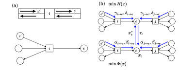
Figure 1: (a) Top: a directed road network section with a junction node $i$. Bottom: the corresponding factor graph representation; node $i$ is a factor node and is marked by a square. (b) Bilevel MP for toll planning. Blue arrows indicate the directions of messages. The equilibrium flow $x_{e}^{*}$ is determined in the lower level, while the toll $\tau_{e}$ is set in the upper level.

The lower-level optimization is a nonlinear min-cost flow problem, where edge flows are coupled through the conservation constraints in Eq. (1), represented as factor nodes in Fig. 1(a). We employ the MP approach developed in Ref. Wong and Saad (2007) to tackle the nonlinear optimization problem. It turns the global optimization of the potential into a local computation of the following message functions

$$\Phi_{i\to e}(x_{e})=\min_{\{x_{e^{\prime}}\geq 0\}|R_{i}=0}\sum_{e^{\prime}\in\partial i\backslash e}\bigg{[}\Phi_{e^{\prime}\to i}(x_{e^{\prime}})+\phi_{e^{\prime}}(x_{e^{\prime}})\bigg{]},$$ (2)

where $\partial i=\partial_{i}^{\text{in}}\cup\partial_{i}^{\text{out}}$ and $\Phi_{i\to e}(x_{e})$ relates to the optimal potential function contributed by the flows adjacent to node $i$ where the flow on edge $e$ is set to $x_{e}$, taking into account flow conservation at node $i$. In Eq. (2), denoting $e^{\prime}=(k,i)$, we can write $\Phi_{e^{\prime}\to i}(x_{e^{\prime}})=\Phi_{k\to e^{\prime}}(x_{e^{\prime}})$; therefore only factor-to-variable messages are needed. The message $\Phi_{k\to e^{\prime}}(x_{e^{\prime}})$ can be obtained recursively by an expression similar to Eq. (2), but using the incoming messages from its upstream edges $\{l\to k|(l,k)\in\partial k\backslash i\}$. Upon computing the messages iteratively until convergence, we can determine the equilibrium flow $x_{e}^{*}$ on edge $e=(i,j)$ by minimizing the edgewise full energy dictated by the nonlinear cost $\phi_{e}(x_{e})$ and messages from both ends of edge $e$, defined as $\Phi_{e}^{\text{full}}(x_{e})=\Phi_{i\to e}(x_{e})+\Phi_{j\to e}(x_{e})+\phi_{e}(x_{e})$.

This algorithm can be demanding when different values of $x_{e}$ are needed to determine the profile of the message $\Phi_{i\to e}(x_{e})$. To reduce the computational cost, we consider the approximation of the message in the vicinity of some working point $\tilde{x}_{i\to e}$ as

$$\Phi_{i\to e}(\tilde{x}_{i\to e}+\varepsilon_{e})\approx\text{$\Phi_{i\to e}$($\tilde{x}_{i\to e}$})+\beta_{i\to e}\varepsilon_{e}+\frac{1}{2}\alpha_{i\to e}\big{(}\varepsilon_{e}\big{)}^{2},$$ (3)

where $\beta_{i\to e}$ and $\alpha_{i\to e}$ are the first and second derivatives of $\Phi_{i\to e}$ evaluated at $\tilde{x}_{i\to e}$, assuming the derivatives exist. For a particular $\tilde{x}_{i\to e}$, the computation of the message function $\Phi_{i\to e}(x_{e})$ in Eq. (2) reduces to the optimization of $\beta_{i\to e}$ and $\alpha_{i\to e}$ by using $\{\tilde{x}_{k\to e^{\prime}},\beta_{k\to e^{\prime}},\alpha_{k\to e^{\prime}}|e^{\prime}=(k,i)\in\partial i\backslash e\}$. The working point $\tilde{x}_{i\to e}$ is updated by pushing it towards the minimizer $x_{e}^{*}$ of the full energy $\Phi_{e}^{\text{full}}(x_{e})$ gradually BoL . The iterative updates of the coefficients $\{\beta_{i\to e},\alpha_{i\to e}\}$ and the working points $\{\tilde{x}_{i\to e}\}$ constitute a perturbative version of the original MP algorithm, which only requires to keep track of a few coefficients rather than the full profile of $\Phi_{i\to e}$, making it tractable Wong and Saad (2007). It has been shown to work remarkably well in many network flow problems Wong et al. (2016), while the algorithm may not converge in problems with nonsmooth characteristics Wong and Saad (2007). We discover that the non-negativity constraints on flows can result in a nonsmooth message function $\Phi_{i\to e}(x_{e})$, which makes the approximation of Eq. (3) inadequate. One solution is to approximate $\Phi_{i\to e}(x_{e})$ by a continuous and piecewise quadratic function with at most two branches, where each branch $m$ is a quadratic function governed by three coefficients $\{\tilde{x}_{i\to e},\beta_{i\to e}^{(m)},\alpha_{i\to e}^{(m)}\}$, as illustrated in Fig. 2(a). Taking into account the nonsmooth structures, MP algorithms converge well even in loopy networks and provide the correct solutions BoL . We demonstrate the case of random regular graphs (RRG) with degree 3 in Fig. 2(b).

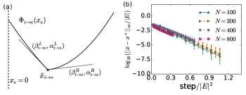
Figure 2: (a) A nonsmooth message function $\Phi_{i\to e}(x_{e})$ with one breakpoint. (b) Convergence of the single-level MP algorithm for computing equilibrium flows in routing games in random regular graphs with degree 3 of different sizes $N=|V|$. An affine latency model $\ell_{e}(x_{e})=t_{e}(1+sx_{e}/c_{e})$ is considered, where $t_{e}$ and $c_{e}$ are the free traveling time and edge capacity, respectively, while $s$ is a sensitivity measure of latency to congestion Roughgarden (2005). Random sequential schedule of MP updates has been used.

For bilevel optimization, we notice that the cost function of the upper layer $H(x)$ has a similar structure as $\Phi(x)$. Therefore, one can apply a similar MP procedure as $H_{i\to e}(x_{e})=\min_{\{x_{e^{\prime}}\}|R_{i}=0}\sum_{e^{\prime}\in\partial i\backslash e}[H_{e^{\prime}\to i}(x_{e^{\prime}})+x_{e^{\prime}}\ell_{e}(x_{e^{\prime}})]$. The message $H_{i\to e}(x_{e})$ can also be approximated by a piecewise quadratic function with at most one break point, where each branch $m$ has the form $H_{i\to e}^{(m)}(\tilde{x}_{i\to e}+\varepsilon_{e})\approx\text{$H_{i\to e}^{(m)}$($\tilde{x}_{i\to e}$})+\gamma_{i\to e}^{(m)}\varepsilon_{e}+\frac{1}{2}\delta_{i\to e}^{(m)}\big{(}\varepsilon_{e}\big{)}^{2}$. As the equilibrium state is determined in the lower level, the working points $\{\tilde{x}_{i\to e}\}$ in the lower-level MP are also used for the upper level. The landscape of the edgewise full cost $H_{e}^{\text{full}}(x_{e})=H_{i\to e}(x_{e})+H_{j\to e}(x_{e})+x_{e}\ell(x_{e})$ provides the information for setting the toll. Specifically, the toll is updated by $\min_{\tau_{e}}H_{e}^{\text{full}}(x_{e}^{*}(\tau_{e}))$, where the toll-dependent equilibrium flow $x_{e}^{*}$ is provided by the lower-level messages. In practice, an approximate $H_{e}^{\text{full}}$ is sufficiently informative for updating tolls. The basic structure of such bilevel MP is illustrated in Fig. 1(b), while details are provided in the SM BoL .

We demonstrate the effectiveness of the proposed bilevel MP algorithm for tasks on RRG in Fig. 3(a), where the set-up is the same as in Fig. 2(b). Experiments on other networks and the cases of multiple destinations are discussed in the SM BoL . Although bilevel message-passing does not generally converge to a set of unique optimal tolls due to the non-convex nature of the problem, we found that the social costs are reduced when tolls are updated during MP. The scaling relation in the inset of Fig. 3(a) empirically indicates that the number of updates is $O(|E|^{2})$ for achieving a given cost reduction. Moreover, the MP algorithm can be implemented in a fully distributed manner, unlike the generic global optimization approach BoL . Note that we have utilized the special set-up of routing games here, where the social optimum $H_{S}=\min_{x}H(x)$ can be obtained a priori for this benchmark. Such information may be unavailable in other bilevel-optimization problems. The toll optimization problem can also be tackled by the bilevel programming approach Bard and Falk (1982); Bard (1988); however, it requires a treatment with mixed integer programming, which is centralized and generally not scalable, unlike the MP approach BoL .

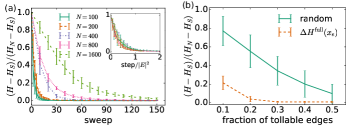
Figure 3: Bilevel MP algorithm for routing games on RRG. (a) Effect of tolls on the fractional social cost reduction $(H(\boldsymbol{x}^{*}(\boldsymbol{\tau}))-H_{S})/(H_{N}-H_{S})$, where $H_{S}$ and $H_{N}$ represent the social costs at the social optimum and the Nash equilibrium without tolls. Tolls $\boldsymbol{\tau}$ are recorded during bilevel MP updates, based on the resulting equilibrium flows $\boldsymbol{x}^{*}(\boldsymbol{\tau})$ and social cost $H(\boldsymbol{x}^{*}(\boldsymbol{\tau}))$. Each data point is the average of 10 different problem realizations. Each sweep consists of $40|E|$ local MP steps and $100$ edgewise toll updates in a random sequential schedule. A fixed number of sweeps without toll updates are performed to warm up the system. Inset: panel (a) with $x$-axis as MP steps rescaled by $|E|^{2}$. (b) Fractional cost reduction as a function of the fraction of tollable edges on an RRG with $N=200$. A random selection of edges to be charged is compared with selections based on edgewise full cost reduction $H_{e}^{\text{full}}(x_{e}^{*})$.

Combinatorial Problems. In practice, it may be infeasible to charge for every edge, but desirable to choose a subset of tollable edges for toll-setting Hoefer et al. (2008), which is a difficult combinatorial optimization problem. As the cost landscape is manifested locally by the message functions, we heuristically select the tollable edges according to the largest possible reduction in edgewise full cost $H_{e}^{\text{full}}(x_{e}^{*})$ due to tolling, which effectively selects the chargeable links as seen in Fig. 3(b). Such combinatorial problems are generally very difficult for traditional bilevel-optimization methods, while MP algorithms can provide approximate solutions in some scenarios.

Another important class of combinatorial problems is the atomic games which consider integer flow variables $\{x_{e}\}$ Rosenthal (1973). In principle, atomic games can be solved via the same MP procedure as in Eq. (2), where the message $\Phi_{i\to e}(x_{e})$ is defined on a one dimensional grid. Using the techniques in Refs. Yeung and Saad (2012); Yeung (2013); Bacco et al. (2014); Yeung et al. (2013); Po et al. (2021), the MP approach provides a scalable algorithm to approximately tackle the difficult combinatorial optimization of atomic games in a single level; it can also solve instances of the bilevel toll-optimization problems. However, its performance is sub-optimal in large networks and for cases with heavy loads BoL . Nevertheless, we found some interesting patterns of the optimal tolls in a realistic test case network using this method BoL .

Flow Control. We consider the problem of tuning network flows to achieve certain functionality. In this example, resources need to be transported from source nodes to destination along edges in an undirected network $G(V,E)$, where the equilibrium flows $\{x_{ij}^{*}\}$ minimize the transportation cost $C=\sum_{(i,j)\in E}\frac{1}{2}r_{ij}x_{ij}^{2}$, subject to flow conservation constraints similar to Eq. (1). The major difference of this model from routing games is that the network is undirected, where edge $(i,j)$ can accommodate either the flow from node $j$ to $i$ or $i$ to $j$. The objective is to control the parameters $\{r_{ij}\}$ to reduce or increase the flows on some edges. The task of reducing edge flows has applications in power grid congestion mitigation in the direct-current (DC) approximation Wood et al. (2013), where $r_{ij}$ is related to the reactance of edge $(i,j)$, controllable through devices in a flexible alternating current transmission system (FACTS) Zhang et al. (2006). On the other hand, the task of increasing certain edge flows has been used to model the tunability of network functions, which is applicable in mechanical and biological networks Rocks et al. (2019) as well as learning machines in metamaterials Stern et al. (2021).

As an example, we consider the task of flow control such that the relative increments of flows on the targeted edges $\mathcal{T}$ exceed a limit $\theta$ Rocks et al. (2019), i.e., $\rho_{ij}=\frac{|x_{ij}|-|x_{ij}^{0}|}{|x_{ij}^{0}|}-\theta\geq 0,\forall(i,j)\in\mathcal{T}$ (with $x_{ij}^{0}$ being the flow prior to tuning). It can be achieved by minimizing the hinge loss (upper-level objective) $\mathcal{O}=\sum_{(i,j)\in\mathcal{T}}-\rho_{ij}\Theta(-\rho_{ij})=:\sum_{(i,j)\in\mathcal{T}}\mathcal{O}_{ij}$, where $\Theta(\cdot)$ is the Heaviside step function. The task of congestion mitigation in power grids can be studied similarly. We adopt the usual MP algorithm to compute the equilibrium flows as

$$C_{i\to j}(x_{ij})=\min_{\{x_{ki}\}|R_{i}=0}\bigg{[}\frac{1}{2}r_{ij}x_{ij}^{2}+\sum_{k\in\mathcal{N}_{i}\backslash j}C_{k\to i}(x_{ki})\bigg{]},$$ (4)

where $\mathcal{N}_{i}$ is the set of neighboring nodes adjacent to node $i$. The definition of the message $C_{i\to j}(x_{ij})$ differs from the one of Eq. (2) in that it includes the interaction term on edge $(i,j)$, which yields a more concise update rule here. Similar to Eq. (3), we approximate the message function by a quadratic form $C_{i\to j}(x_{ij})=\frac{1}{2}\alpha_{i\to j}(x_{ij}-\hat{x}_{i\to j})^{2}+\text{const}$, such that the optimization in Eq. (4) reduces to the computation of the real-valued messages $m_{i\to j}\in\{\alpha_{i\to j},\hat{x}_{i\to j}\}$ by passing the upstream messages $\{m_{k\to i}\}_{k\in\mathcal{N}_{i}\backslash j}$, as illustrated on the left panel of Fig. 4(a) BoL . Upon convergence, the equilibrium flow $x_{ij}^{*}$ can be obtained by minimizing the edgewise full cost $C_{ij}^{\text{full}}(x_{ij})=C_{i\to j}(x_{ij})+C_{j\to i}(x_{ij})-\frac{1}{2}r_{ij}x_{ij}^{2}$.

The variation of the control parameters $\{r_{ij}\}$ will impact on the messages $\{m_{i\to j}\}$, which in turn affects the equilibrium flows $\boldsymbol{x}^{*}$ and therefore the upper-level objective $\mathcal{O}(\boldsymbol{x}^{*})$. Specifically, one considers the effect of the change of $r_{ij}$ on the targeted edge flows $\{x_{pq}^{*}\}_{(p,q)\in\mathcal{T}}$, derived by computing the gradient $\frac{\partial\mathcal{O}}{\partial m_{i\to j}}$. The targeted edges provide the boundary conditions as $\frac{\partial\mathcal{O}_{pq}}{\partial m_{p\to q}}=\frac{\partial\mathcal{O}_{pq}}{\partial x_{pq}^{*}}\frac{\partial x_{pq}^{*}}{\partial m_{p\to q}},\forall(p,q)\in\mathcal{T}$. As the messages from node $i$ to $j$ are functions of the upstream messages, i.e., $m_{i\to j}=m_{i\to j}(\{m_{k\to i}\}_{k\in\mathcal{N}_{i}\backslash j})$, the gradients on edge $i\to j$ are passed backward to its upstream edges $\{k\to i\}_{k\in\mathcal{N}_{i}\backslash j}$ through the chain rule, as illustrated in the right panel of Fig. 4(a). The full gradient on a non-targeted edge $k\to i$ can be obtained by summing the gradients on its downstream edges, computed as

$$\frac{\partial\mathcal{O}}{\partial m_{k\to i}}=\sum_{l\in\mathcal{N}_{i}\backslash k}\,\,\sum_{m_{i\to l}\in\{\alpha_{i\to l},\hat{x}_{i\to l}\}}\frac{\partial\mathcal{O}}{\partial m_{i\to l}}\frac{\partial m_{i\to l}}{\partial m_{k\to i}}.$$ (5)

The gradient messages $\{\frac{\partial\mathcal{O}}{\partial m_{k\to i}}\}$ are passed in a random and asynchronous manner, resulting in a decentralized algorithm.

The gradient with respect to the control parameter on the non-targeted edge $(k,i)$ can be obtained straightforwardly as

$$\frac{\partial\mathcal{O}}{\partial r_{ki}}=\sum_{m\in\{\alpha,\hat{x}\}}\bigg{(}\frac{\partial\mathcal{O}}{\partial m_{k\to i}}\frac{\partial m_{k\to i}}{\partial r_{ki}}+\frac{\partial\mathcal{O}}{\partial m_{i\to k}}\frac{\partial m_{i\to k}}{\partial r_{ki}}\bigg{)},$$ (6)

which serves to update the control parameter in a gradient descent manner $r_{ki}\leftarrow r_{ki}-s\frac{\partial\mathcal{O}}{\partial r_{ki}}$ with certain step size $s$. The gradient for targeted edges can be similarly defined BoL . The control parameters are bounded to be $r_{ij}\in[0.9,1.1]$, achieved by necessary thresholding after gradient descent updates. In this flow model, the gradient $\frac{\partial\mathcal{O}}{\partial r_{ki}}$ can be calculated exactly, leading to a global gradient descent (GGD) algorithm. However, the GGD approach requires computing the inverse of the Laplacian matrix in every iteration, which can be time-consuming for large networks. On the contrary, the gradients are computed in a local and distributed manner in the MP approach. Similar ideas of gradient propagation of MP have been proposed in Refs Eaton and Ghahramani (2009); Domke (2013) in the context of approximate inference, which are usually implemented centrally in the reversed order of MP updates, unlike the decentralized approach presented here.

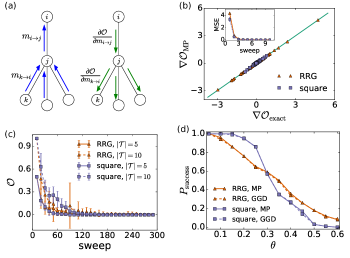
Figure 4: Bilevel optimization for flow control. An RRG ($N=200$, degree $3$) and a square lattice of size $15\times 15$ are considered. The source and destination nodes, and the targeted edges are randomly selected. (a) Left: MP for solving the lower-level equilibrium flow problem. Right: Computing gradients of the upper-level objective function $\mathcal{O}$. (b) Comparison of the gradients at initial $\boldsymbol{r}$ computed by the MP approach (obtained by fixing $\boldsymbol{r}$ and passing messages $\{m_{i\to j}\}$ and gradients $\{\frac{\partial\mathcal{O}}{\partial m_{i\to j}}\}$) and the GGD approach, with $|\mathcal{T}|=5,\theta=0.1$. Inset: mean square error (MSE) of the gradients by the MP approach during iterations, in comparison to the GGD approach. Each sweep consists of $4|E|$ local MP steps. (c) MP for minimizing the upper-level objective function $\mathcal{O}$ with $\theta=0.1$, where one randomly selected control parameter is updated following the descent direction every $4|E|/10$ steps. (d) Fraction of successfully tuned cases (satisfying $\mathcal{O}=0$) $P_{\text{success}}$ out of $100$ different problem realizations of source/destination nodes, with $|\mathcal{T}|=5$, as a function of the threshold $\theta$.

The gradient computed by the MP algorithm provides an excellent estimation to the exact gradient, as illustrated in Fig. 4(b). For bilevel optimization, we do not wait for the convergence of the gradient-passing, but update the control parameters during the MP iterations to make the algorithm more efficient. It provides approximated gradient information, which is already effective for optimizing the global objective, as shown in Fig. 4(c). The MP approach yields similar success rates in managing the network flows for different thresholds compared to the GGD approach as shown in Fig. 4(d), demonstrating the effectiveness of the MP approach for the bilevel optimization.

In summary, we propose MP algorithms for solving bilevel optimization in flow networks, focusing on applications in the routing game and flow control problems. In routing games, the objective functions in both levels admit a similar structure, which leads to two sets of similar messages being passed. Updates of the control variables based on localized information appear effective for toll optimization. However, the long-range impact of control-variable changes should be considered in some applications. This is accommodated by a separate distributed gradient-passing process, which is effective and efficient in flow control problems. Leveraging the sparse network structure, the MP approach offers efficient and intrinsically distributed algorithms in contrast to global optimization methods such as nonlinear programming, which is more generic, but is generally not scalable and therefore unsuitable for large-scale systems. The MP approach provides effective algorithms for bilevel optimization problems that are intractable or difficult to solve by global optimization approaches, such as combinatorial problems. We believe that these MP methods provide a valuable tool for solving difficult bilevel optimization problems, especially in systems with sparsely coupled structures.

Source codes of this work can be found in https://github.com/boli8/bilevelMP_flow.