An Applied Deep Learning Approach for Estimating Soybean Relative Maturity from UAV Imagery to Aid Plant Breeding Decisions

Abstract

For a global breeding organization, identifying the next generation of superior crops is vital for its success. Recognizing new genetic varieties requires years of in-field testing to gather data about the crop’s yield, pest resistance, heat resistance, etc. At the conclusion of the growing season, organizations need to determine which varieties will be advanced to the next growing season (or sold to farmers) and which ones will be discarded from the candidate pool. Specifically for soybeans, identifying their relative maturity is a vital piece of information used for advancement decisions. However, this trait needs to be physically observed, and there are resource limitations (time, money, etc.) that bottleneck the data collection process. To combat this, breeding organizations are moving toward advanced image capturing devices. In this paper, we develop a robust and automatic approach for estimating the relative maturity of soybeans using a time series of UAV images. An end-to-end hybrid model combining Convolutional Neural Networks (CNN) and Long Short-Term Memory (LSTM) is proposed to extract features and capture the sequential behavior of time series data. The proposed deep learning model was tested on six different environments across the United States. Results suggest the effectiveness of our proposed CNN-LSTM model compared to the local regression method. Furthermore, we demonstrate how this newfound information can be used to aid in plant breeding advancement decisions.

1 Introduction

Agriculture has been one of the most critical industries since human civilization. From manual-powered efforts thousands of years ago to the modern large-scale machine-driven farming, this industry is evolving to feed the increasing population while facing limited resources. In agriculture, soybeans (Glycine max) rank among one of the most important crops worldwide (Lee et al., 2015; Pagano and Miransari, 2016). Soybeans are not only a key source of protein for humans and livestock but also a key ingredient for biodiesel and vegetable oils. In 2019, the United States soybean exports totaled 19 billion USD with the global soybean market estimated to be over 50 billion USD each year since 2015 (USDA, 2019).

Given the economic impact of soybeans, breeding companies, both in the private and public sector, endeavor to release improved soybean varieties to meet market demands where these new varieties are hopefully higher yielding than the previous generation. The process to identify superior varieties is through years of observed field trials. Within all soybean breeding pipelines, the relative maturity of a genetic soybean variety is an important characteristic to determine optimal growing environments, based mostly on latitude (Ortel et al., 2020). Identifying a soybean’s relative maturity enables plant breeders to make optimal planting placement decisions to ensure a soybean reaches its maximum growth potential. That is, placing a genetic soybean variety in the correct latitude band will allow for the proper accumulation of sunlight needed for optimal growth. If a soybean variety is not placed into its optimal growing environment, the soybean may freeze before harvest, ultimately wasting precious resources and its yield potential. For a commercial breeding organization, at the end of each growing season, soybean advancement decisions must be made to determine which soybeans will be chosen to progress towards another year of field testing and which ones will be discarded. These meetings are typically considered the backbone of any breeding organization, and a company’s success depends on identifying the best crops to move forward. It is common for these decisions to encompass 40,000 genetically different soybean varieties, and having key information is the difference between a confident decision and an educated guess. Soybean relative maturity is one of the most important factors (in addition to yield) in determining if a soybean is advanced or not. Therefore, it is vital that this information is accurately and efficiently collected before these decisions need to be made.

To determine the relative maturity of a soybean variety, soybean field trials are manually screened approximately once or twice per week by soybean physiology experts to determine the day of the year that 95% of soybean pods within a plot have reached their mature brown color (Fehr and Caviness, 1977). However, for a global breeding organization, manually screening soybean fields is labor-intensive, time-consuming, and prone to human error, making the data collection process a difficult task. Of the 40,000 genetically different soybean varieties, only a fraction will have their relative maturity identified, leading to less optimal advancement decisions.

In recent years, digital and data-driven breeding/farming has led agriculture to a new era (Yost et al., 2011; Aubert et al., 2012; Kurkalova and Carter, 2017; Karimzadeh and Olafsson, 2019; Shahhosseini and Hu, 2020; Moeinizade et al., 2019, 2020a, 2021; Emirhüseyinoğlu and Ryan, 2020; Amini et al., 2021; Han et al., 2021). Satellite imaging, live GPS tracking, drone-based fertilizing and screening, micro-sensors in the soil, etc., are all examples of new techniques that have brought significant changes to the agricultural industry. Modern image capturing devices such as unmanned aerial vehicles (UAVs) allow researchers to gather images of crop fields at a faster rate with reduced dependency on error-prone, manual labor. Combined with modern analytical techniques, these images provide crop level data that breeders and farmers can use to enhance decision making (Nguyen et al., 2020; Peng et al., 2020; Khaki et al., 2021b). A scalable image capturing technology has the ability to increase information throughput as well as reduce human error. However, the adoption of a new process leads to a new set of challenges, such as when and how frequently images should be collected and how algorithms can be trained to best convert images into useful data for decision making. Oftentimes, the turnaround from the last drone flight to the advancement decision deadline is a couple of days. Therefore, any established data pipeline needs to be scalable to provide efficient data turnaround that is accurate for end goal needs.

Within machine learning, deep neural networks (DNN) are commonly used models that contain many sequentially stacked layers allowing the model to learn features that encode information from the image. Using a DNN, features are automatically learned from input data without manual feature creation. With increased computing power, automating image analysis is possible for agricultural tasks such as image classification, object detection, and object counting. These approaches often rely on a special type of DNN called convolutional neural networks (CNN). CNNs excel at image-based tasks because they take advantage of the spatial structure of the pixels. Additionally, CNNs require a fewer number of learned parameters, achieve superior computational performance compared to traditional machine learning, and reduce the risk of overfitting (O’Shea and Nash, 2015). Given the flexibility and strength of CNNs, it comes as no surprise the vast amount of domains and applications in which they are used (Heinrich et al., 2021; Liu et al., 2021; Tang and Röllin, 2021).

Cornerstone deep learning frameworks such as RetinaNet (Alon et al., 2019), Mask-RCNN (Yu et al., 2019b), and YOLO (Mosley et al., 2020) have been applied to detect sorghum heads, count strawberries, and classify tree species. Also given that commercial corn is a staple crop around the world due to being used for animal feed and biofuels, it is no surprise that there is substantial work combining corn images and deep learning (Khaki et al., 2020a, b, 2021a). Aside from deep learning, many other researchers have combined traditional statistical modeling, machine learning, and image processing with agricultural data (Singh et al., 2016; Naik et al., 2017; Moeinizade, 2018; Dobbels and Lorenz, 2019; Moeinizade et al., 2020b; Pothen and Pai, 2020; Li et al., 2020; Volpato et al., 2021; Shahhosseini et al., 2019, 2020, 2021). With the rapid combination of analytical techniques and plant breeding, this large body of recent work illustrate that large-scale analysis of imagery for improved decision making is possible.

Soybean relative maturity is an excellent example of a trait that can be measured using image analysis techniques. Recent efforts have used drone-based imagery to estimate the days to soybean maturity, that is, the day of the year in which 95% of pods within a plot have turned to their mature brown color. These approaches have relied on multiple linear regression (Christenson et al., 2016), LOESS regression (Volpato et al., 2021), segmented regression (Narayanan et al., 2019), and partial least squares regression (Zhou et al., 2019). Each of these methods relies on condensing each RGB image to a single value, such as the normalized difference vegetation index or the green leaf index. However, such an approach lends itself to information loss due to summarizing a complete image towards a single number. Moreover, to date, Trevisan et al. (2020) is the only work that has used a CNN to estimate soybean maturity dates. However, their work does not take into account the temporal relationship between drone flight dates and simply uses an image classification approach. Therefore any extension of the literature requires addressing the temporal relationship between drone images, such as by using a long short term memory (LSTM) recurrent neural network (Yu et al., 2019a). Like a CNN, an LSTM is a special type of deep neural network that can process multiple data points and sequences. Thus, they naturally lend themselves to be used for time series analysis. Given that important decisions depend on the accuracy of these predictions, it is vital that any edge in prediction accuracy is obtained.

Given this information, our research aims to

1. Create a temporal, image-based, deep learning model (CNN-LSTM) to estimate soybean maturity

2. Determine how our model’s accuracy changes under the differing temporal frequency of flights

3. Create a data-driven support system that will inform plant breeders when sufficient UAV imagery is captured for a soybean variety advancement decision

Ideally, throughout a soybean’s growth cycle, a drone flight should be conducted each day. However, in practice, due to limited resources (time, labor, money, etc.) and varying weather conditions, drone images may only be taken at most once or twice a week. Therefore it is the goal of this paper to create a system so that commercial breeding organizations can make decisions on when to best conduct drone flights and identify when enough flights are taken for an accurate soybean maturity date estimation to, ultimately, aid in advancement decisions. Additionally, if a prediction is within $\pm$ two days of the actual maturity date, that is enough to make a confident advancement decision.

2 Methods

In this section, we introduce an end-to-end framework to systematically estimate the relative maturity of soybeans using computer vision and deep learning techniques. Our proposed framework comprises of four phases which are the data extraction and assembly, data pre-processing, feature extraction, and prediction phases. The data extraction and assembly phase first extracts plot images from each flight’s full field orthomosaic and then assembles the time series of plot images for a given date. That is, each variety is snipped into a single image and then sequenced together by drone flight date. The data pre-processing phase includes rotating and resizing images to make the data consistent. In the feature extraction phase, time distributed convolutional neural networks are designed to automatically extract features from the time series of images for each variety. Finally, long short-term memory recurrent neural networks are used to predict the relative maturity of soybeans given features extracted from the previous phase. Figure 1 illustrates this process for a single flight orthomosaic (one drone flight on a single day) for numerous soybean varieties. At each stage, we make use of open-source software for our end-to-end process. In practice, this entire pipeline is completed in an efficient manner, so that plant breeders have sufficient data to make necessary soybean advancement decisions.

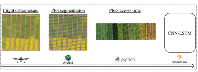
Figure 1: Illustration of the image capturing, data processing, and prediction process

2.1 Proposed deep learning model

Figure 2 demonstrates the structure of the deep learning model. In this hybrid model, for each plot snip, time-distributed CNNs are used for deep feature extraction, and LSTM is used for capturing the sequential behavior of time series data. Time distributed layers have the advantage of applying convolution on each image in the time series independently.

In detail, each image is first passed to a set of convolutional and max pooling layers to produce a fixed-length vector representation. Convolutional layers act as a feature extractor that automatically learns specific details about the image. This contrasts with traditional machine learning methods, where features need to be handcrafted by a domain expert. Acting as our feature extractor, we have four convolutional layers and two max pooling layers. The repetitive nature of the convolutions helps to extract a more detailed structure about the images. As an illustration, the first couple of convolutional layers learn simple features such as colors and edges, but as the number of convolutions increase, the new features identify shading patterns, areas of interest, and pixel densities. At a high level, the max pooling layers act to reduce the dimensions from learned feature maps, and therefore reduce the number of parameters to learn, thus leading to less computational demand. In short, the convolutional layers act as a way to reduce an image down to a single vector of features so that the resulting output can be read into a learning algorithm.

Figure 3 demonstrates the architecture of CNN layers (see section 3.3 for more details about the network architecture). The outputs of CNN for the sequence of plot images are passed to an LSTM model. Long short-term memory (LSTM) is a special type of recurrent neural network (RNN) that is well suited for making predictions based on time series data. LSTMs solve the vanishing gradient problem that can be encountered in classical RNNs by using information gates to store useful information and forget unnecessary information. The output of the LSTM layer is passed to an output layer, and finally, relative maturity is estimated. More instructions about experiment design are presented in section 3.3.

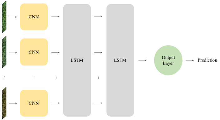
Figure 2: The CNN-LSTM structure used to predict soybean relative maturity from images.

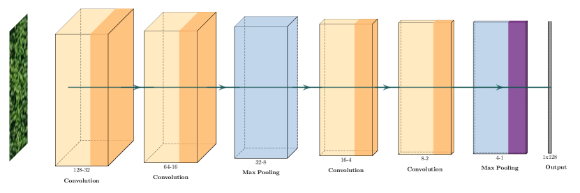
Figure 3: Illustration of the CNN architecture. The convolution layers apply convolution operation between the raw data and convolution kernels producing new features. The numerical values represent the dimensions of each layer (depth-width). The max pooling layers are down sampling the convolved features and help to make the system more robust since small changes of the input will not change the pooling output.

2.1.1 Loss Function

To make the model more robust to outliers, we used Huber loss function (Huber, 1992) which is defined as follows:

$$L_{\delta}(y,\hat{y})=\left\{\begin{array}[]{ll}\frac{1}{2}(y-\hat{y})^{2}&\text{ for }\ |y-\hat{y}|\leq\delta\\ \delta|y-\hat{y}|-\frac{1}{2}\delta^{2}&\text{ otherwise }\end{array}\right.$$ (1)

Here $y$ is the true label, and $\hat{y}$ is the prediction. For small values of $\delta$, this function is quadratic and for large values it is linear. Moreover, $\delta$ is a hyper-parameter that can be tuned. This loss function brings the advantages of mean square error (MSE) loss and mean absolute error (MAE) loss together by combining them in a piecewise manner.

2.2 Benchmark

We compare the performance of our proposed deep learning model against a recent state-of-the-art benchmark created by Volpato et al. (2021) where a local regression model is fitted to the RGB color transformation values over time. That is, for each plot and drone flight date, an RGB transformation is performed, and the output is fed into the regression model. Volpato et al. (2021) demonstrated that using the mean greenness leaf index (GLI) on each plot combined with locally estimated scatter plot smoothing (LOESS) regression results in higher correlations between the predicted and ground truth maturity days. The LOESS model combines much of the simplicity of linear least squares regression with the flexibility of nonlinear regression by fitting linear models to localized subsets of data determined by a nearest neighbor algorithm (Cleveland and Devlin, 1988). In this study, the LOESS model was implemented using the “lowess” function from “statmodels” package in Python to interpolate the GLI values extracted from the time series of images. This function implements the algorithm described in Cleveland (1979). The GLI index can be calculated as follows:

$$GLI=\frac{2G-R-B}{2G+R+B}$$ (2)

where R, G, and B are the mean values of red, green, and blue channels respectively for each image. Finally, the relative maturity date is predicted as the day with the closest value to a predefined threshold, where the threshold value corresponds to a level of greenness. Volpato et al. (2021) suggested that a GLI threshold of 0.02 was optimal from their extensive testing. However, this value can vary based on the environment and equipment, and optimizing a single threshold is not scalable. This is one limitation we hope to address with our CNN-LSTM approach.

3 Experiments and Results

In this section, we present the data sets used in this study, the deep learning model’s hyper-parameter tuning, and the results for both the deep learning model and the LOESS model.

3.1 Data

Data from 6 different locations across the United States in two growing seasons (2018 and 2019) is used in this study. All data (orthomosaics, plot delineations, and ground-truth) except environment 3 (Elkhart, IA, 2019) were adopted from the University of Minnesota Soybean breeding project (Lorenz, 2020). The environment 3 data set is provided by a commercial breeding organization. The following table includes more details about the data sets used in this study. Environments 3 and 6 have the largest number of plots (soybean varieties), which is almost twice the number of plots in other environments. During the growing season, a commercial breeding organization can have upwards of 40,000 genetically different soybeans planted in 200 geographically different locations (ranging from Mississippi to Canada). Due to the labor requirements and plant breeding expertise needed to accurately observe soybean maturity, it is challenging to have extensive ground-truth data.

Environment	Location	Year	Number of plots	Planting date	UAS Platform
1	Waseca, MN	2018	874	May 17	DJI Phantom 3 Pro
2	Lamberton, MN	2018	796	May 16	DJI Phantom 3 Pro
3	Elkhart, IA	2019	1686	April 24	DJI Phantom 3 Pro
4	Waseca, MN	2019	688	May 15	DJI Phantom 3 Pro
5	Lamberton, MN	2019	896	May 16	DJI Phantom 3 Pro
6	Rosemount, MN	2019	1410	May 26	DJI Inspire 1

Table 1: Data set descriptions. Each environment varies in number of plots, planting dates and unmanned aircraft system (UAS) platform.

Each data set includes orthomosaics, plot boundary delineations, ground control points, and the ground-truth notes that were taken by soybean physiology experts visiting plots and manually observing the soybean’s relative maturity. To extract individual plots from orthomosaic images, we used a Python script to parse the plot boundaries, and we tagged each image with the drone flight date and unique identifier (soybean’s name). We performed this process for each orthomosaic across all flight dates as shown in Table 2. In total, we processed 31,750 unique images. It should be noted that the number of plots is not exactly the same as the previous work conducted by Volpato et al. (2021) since we kept outliers in the data sets to test the robustness of our proposed models. Whereas Volpato et al. (2021) removed outliers.

Environment	Flight dates
1	Sep 6, Sep 13, Sep 20, Sep 27, Oct 8
2	Sep 5, Sep 14, Sep 17, Sep 25, Oct 4
3	Sep 7, Sep 13, Sep 20, Sep 26, Oct 3
4	Sep 6, Sep 14, Sep 21, Sep 27, Oct 7
5	Sep 6, Sep 14, Sep 18, Sep 25, Oct 4
6	Sep 6, Sep 13, Sep 20, Sep 27, Oct 7

Table 2: Flight dates across 6 environments. For each environment, 5 images are selected on a weekly basis starting from September till the first week of October. Bi-weekly images can be obtained by selecting the first, middle and last dates among these flights.

The relative maturity days are calculated as the number of calendar days after August 31. That is, our model simply estimates a numeric value that we add to August 31 to get a month-day estimation for the maturity date. Figure 4 visualizes the distribution of relative maturity days for each environment. As shown in Figure 4 distributions vary in shape and spread. The median of relative maturity days across these 6 environments is 20, 24, 15, 25, 26, and 27, respectively. As expected, environment 3 (with the earliest planting date) has the lowest median, that is, the earliest maturity date.

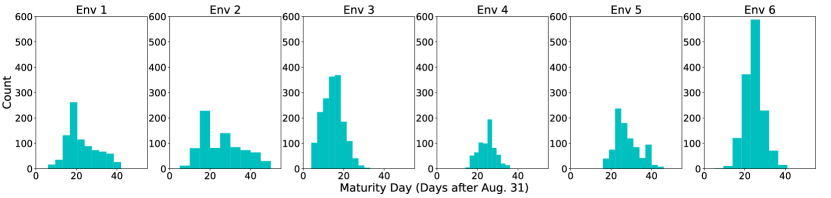
Figure 4: Histograms of relative maturity days for 6 environments. Relative maturity day is defined as days since August 31.

All flights start from mid-August and last in mid-October, and each environment varies in flight dates. To be consistent, we selected weekly flights considering a 5-week period, including 4 weeks in September and the first week of October for each environment. We train our models on weekly and bi-weekly flights, including 5 and 3 images, respectively, to investigate the effect of less frequent flights on prediction performance. In practice, if accurate performance can be obtained from fewer flights, that would increase the speed of information gain, thus allowing sufficient time for plant breeders to make advancement decisions. Operationally, a reduced frequency in the number of drone flights would present significant cost savings both in time and reduce drone costs. In an ideal scenario, a breeding organization can fly drones every day, but due to restrictive factors (weather, time, labor, etc.), flights can only be conducted at most once or twice a week. A system that can yield accurate and confident results with fewer drone flights would have numerous positive outcomes for a breeding organization.

3.2 Data Processing

A number of pre-processing steps are applied to the images before moving on to the prediction task. The first step is to resize all images to a fixed width and length. The original images of plots have a rectangular shape with width varying from 57 to 65 and length varying from 146 to 280. We tried different sizes and find out that the prediction is not very sensitive to the image size since we are mostly extracting features related to color and shape. Therefore, we decided to resize all images to a fixed size of $64\times 256$ for consistency.

Next, we applied some data augmentation techniques to test the robustness of the proposed deep learning model against some variation of images which can be caused due to cloudiness and the relative position between the camera and sun. These techniques include changing the brightness and contrast and making some images blur. Data augmentation techniques have been conducted on 20% of total images. To change the brightness of images, we added a constant to each pixel. Similarly, contrast can be changed by multiplying each pixel by a constant. To make the images blur, we used Gaussian smoothing to remove noise.

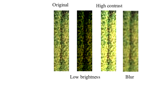
Figure 5: Representation of data augmentation for a single plot. To make an image dark, a negative constant (-100) is added to each pixel of the image (low brightness). High contrast image is obtained by multiplying each pixel by a constant (1.5) and the blur image is obtained by removing noise using guassian blur.

3.3 Design of Experiments

The CNN-LSTM model consists of four time-distributed convolutional layers of 32 filters and two LSTM layers. The detailed structure of the network is provided in Table 3. In the CNN model, downsampling is performed by max pooling with a stride of 2. The output of the last max pooling layer is flattened and used as input features for LSTM layers. The LSTM model has 256 hidden units. The first LSTM layer (LSTM₁) returns a sequence that goes as input to the second LSTM layer (LSTM₂) that outputs a vector. Finally, a dense layer with 1 neuron is applied to estimate the relative maturity of each plot. After trying different network designs, we found this architecture to provide the best overall performance. This architecture has a total of 948,449 trainable parameters.

The weights of the network are initialized using Xavier initialization (Glorot and Bengio, 2010), and activation functions are all rectified linear units (ReLU) except for the last layer, which is linear. The hyperparameter $\delta$ in the Huber loss function is set as 1. To determine this value, we applied a search grid over different values of $\delta$ and chose the optimal one. The loss function is optimized using stochastic gradient descent (SGD) with a batch size of 64 (LeCun et al., 1998). The optimization algorithm is Adaptive Moment Estimation (Adam) with a learning rate of $10^{-3}$ and decay rate of $10^{-1}$ (Kingma and Ba, 2014). The model is trained for 300 iterations.

The proposed model was implemented in Python using the Keras library with the Tensorflow backend, and training time took about half an hour on an NVIDIA Tesla V100 SXM2 GPU.

Layer name	Filter size	# Filters	Stride	Padding	Input size
Time distributed Conv2D1	$3\times 3$	32	2	Same	(5, 256, 64, 3)
Time distributed Conv2D2	$3\times 3$	32	2	Same	(5, 128, 32, 32)
Time distributed MaxPooling2D1	$2\times 2$	-	2	-	(5, 64, 16, 32)
Time distributed Conv2D3	$3\times 3$	32	2	Same	(5, 32, 8, 32)
Time distributed Conv2D4	$3\times 3$	32	2	Same	(5, 16, 4, 32)
Time distributed MaxPooling2D2	$2\times 2$	-	2	-	(5, 8, 2, 32)
Time distributed Flatten	$3\times 3$	-	2	-	(5, 4, 1, 32)
LSTM1	$3\times 3$	32	2	Same	(5, 128)
LSTM2	$3\times 3$	32	2	Same	(5, 256)
Dense (1 neuron)	-	-	-	-	256

Table 3: The full summary of our CNN-LSTM network.

According to Table 1 there exists total $N=6350$ plots. We randomly select 85% of plots as the input and use the rest as the test data to evaluate performance. Since the number of plots varies across different environments, we kept approximately 15% of total plots per environment as test data. As such, the test size across the six environments is 117, 112, 260, 104, 134, and 226, respectively. The input data is split into train and validation sets randomly. The validation set (10 % of input data) is used to monitor the training process.

3.4 Performance Evaluation Metrics

To measure the performance of the proposed model, we use the mean absolute error (MAE) and mean squared error (MSE) metrics, which are defined as follows:

$$MAE=\frac{1}{N}\sum_{i=1}^{N}\left|y_{i}^{pred}-y_{i}^{GT}\right|$$ (3)

$$MSE=\frac{1}{N}\sum_{i=1}^{N}\left|y_{i}^{pred}-y_{i}^{GT}\right|^{2}$$ (4)

Here $y_{i}^{GT}$ denotes the true relative maturity for the $i^{\text{th}}$ plot, $y_{i}^{pred}$ denotes the predicted relative maturity, and $N$ is the total number of plots.

3.5 Results

In this section, we provide the final results for the proposed CNN-LSTM model and the benchmark (LOESS model) and compare their performance.

3.5.1 CNN-LSTM Performance

The CNN-LSTM model is trained using weekly and bi-weekly flight images. Figure 6 demonstrates the performance of the deep learning model across six environments using 5 images on a weekly basis. According to the test performance, the $\text{r}^{2}$ between the ground truth and estimated relative maturity days are higher than 0.8 for all environments except environment 6. Environment 6 has achieved an $\text{r}^{2}$ of 0.5 on the test data. Having more outliers and a different UAV platform has resulted in a decrease in performance for this environment.

Environment 3 has the lowest mean absolute error (less than 1 day) amongst all environments. Environments 1, 4, and 5 have achieved a mean absolute error of fewer than 2 days, whereas environments 2 and 6 have a mean absolute error of almost 2 days.

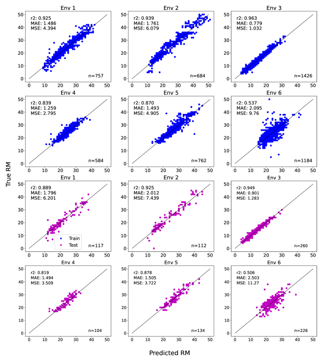
Figure 6: CNN-LSTM model’s train (blue) and test (purple) performance across six environments for 5 images. Figures present the predicted RM versus ground truth. The black line corresponds to $x=y$. The performance metrics are presented in the upper left corner of figures and number of training and test samples are provided in the lower right corner.

Figure 7 presents training and test results across six environments using 3 images. As expected, in most of the cases, $\text{r}^{2}$ has decreased with respect to the previous weekly model. Take, for example, environments 2, 3, 4, 5, and 6 have less $\text{r}^{2}$ compared to the previous model for both train and test sets. However, environment 1 has performed slightly better in terms of all three metrics, which can be explained by highly correlated images.

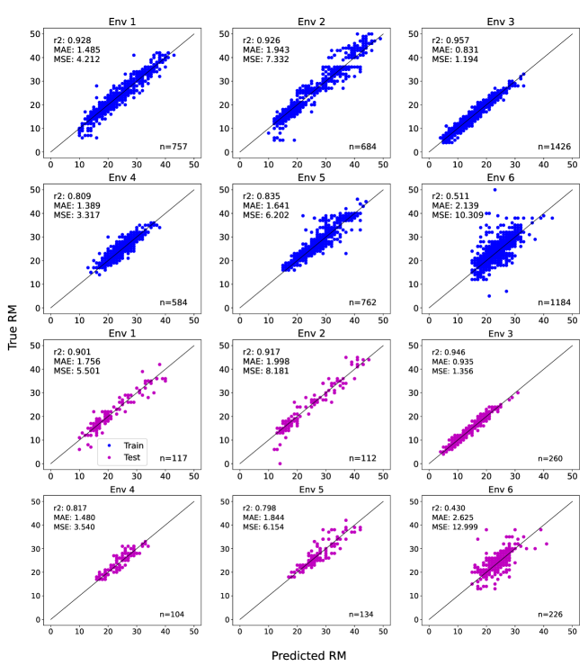
Figure 7: CNN-LSTM model’s train (blue) and test (purple) performance across 6 environments for 3 images.

3.5.2 Comparison

As previously mentioned, the LOESS model depends upon setting a threshold value that is chosen through trial and error. Therefore, we estimate the LOESS model’s performance using 9 different threshold values between 0.01 and 0.09. Detailed results are available in tables 5 and 6 (see appendix). The threshold value corresponding to the best performance differs across environments. Even in some cases, the optimal threshold differs with respect to the chosen metric (see Env2 and Env5 in table 6). Using the LOESS model is difficult in practice due to the sensitivity of identifying the correct threshold. For soybean field trials placed around the entire Midwestern United States, identifying a different threshold value for each environment is not practical and makes scalable implementation difficult.

Table 4 summarizes CNN-LSTM and LOESS performance for both weekly (using 5 images) and bi-weekly (using 3 images) analysis. It should be noted that the LOESS model is fitted to the time series of each plot separately, whereas the deep learning model fits a universal CNN-LSTM on training data and uses the test data for evaluation.

In all cases, the CNN-LSTM model has achieved higher $\text{r}^{2}$ and lower MAE and MSE values, except for environment 1 where LOESS performs slightly better than the CNN-LSTM test performance. For environment 6, the LOESS model is not able to predict any variations on the response ($\text{r}^{2}<0$), whereas the CNN-LSTM model can predict almost 50% of the variation. Furthermore, decreasing the number of input images from 5 to 3 has affected the performance of the LOESS model more than the CNN-LSTM model.

Environment	Metric	Method (Weekly)			Method (Bi-weekly)
		CNN-LSTM		LOESS	CNN-LSTM		LOESS
		Train	Test		Train	Test
1	$\text{r}^{2}$	0.925	0.889	0.906	0.928	0.901	0.851
	MAE	1.486	1.796	1.760	1.485	1.756	2.152
	MSE	4.394	6.201	5.562	4.212	5.501	8.637
2	$\text{r}^{2}$	0.939	0.925	0.788	0.926	0.917	0.746
	MAE	1.761	2.012	3.068	1.943	1.998	3.520
	MSE	6.079	7.439	21.078	7.332	8.181	25.317
3	$\text{r}^{2}$	0.963	0.949	0.940	0.957	0.946	0.908
	MAE	0.779	0.901	0.921	0.831	0.935	1.217
	MSE	1.032	1.283	1.644	1.194	1.356	2.523
4	$\text{r}^{2}$	0.839	0.819	0.719	0.809	0.817	0.313
	MAE	1.259	1.494	1.653	1.389	1.480	2.852
	MSE	2.795	3.509	4.955	3.317	3.540	812.125
5	$\text{r}^{2}$	0.870	0.878	0.759	0.835	0.798	0.616
	MAE	1.493	1.505	2.155	1.641	1.844	3.086
	MSE	4.905	3.722	8.843	6.202	6.154	14.071
6	$\text{r}^{2}$	0.537	0.506	-0.001	0.511	0.430	-0.160
	MAE	2.095	2.503	3.377	2.139	2.625	3.913
	MSE	9.760	11.270	21.362	10.309	12.999	24.770

Table 4: Summary of weekly and bi-weekly analysis using CNN-LSTM and LOESS models. Performance of these two models with respect to three metrics, including $\text{r}^{2}$, MAE, and MSE, is demonstrated across six environments. For the CNN-LSTM model, both train and test performances are reported. For the LOESS model, a search grid is applied to find the optimal threshold, and then the best performance with respect to the corresponding metric is reported.

4 Discussion and Implications

For a commercial plant breeding organization, identifying the maturity date of soybeans is critical. When a soybean’s relative maturity is not classified correctly, it affects harvest operations, can cause seed germination issues, affects advancement decisions, and contributes to a loss in genetic gain. With this approach, we have shown that our CNN-LSTM provides a robust approach to estimating a soybean’s maturity date within $\pm$ 2 days of the actual maturity date without the ambiguity of the LOESS model. That is, we are robust to outliers and do not need to set arbitrary thresholds for prediction. Even using just three drone flights taken two weeks apart for predictions, we achieve high performance accuracy.

The impact of this work demonstrates that drone flights do not need to be conducted every day and that if a drone flight can only be conducted in two week intervals, predictions will still be accurate. This will present itself as a cost saving measure, and no longer do operational specialists have to rush to the field to capture frequent drone flights or even to manually traverse the fields.

Additionally, given the geographical considerations of environment locations, we also notice that some locations may need more drone flights than others, on average. For example, Environment 2 and Environment 6 will need at least 5 drone flights. Whereas Environments 1, 3, 4, and 5 having three drone flights is sufficient. This discrepancy can be attributed to differences in land topography, weather, or soil conditions. This inadvertently leads itself into other plant breeding questions that connect soybean genetics to the environment and farm management practices, all of which are important pieces to consider for soybean advancement.

Moreover, from the perspective of the plant breeder, knowing that an advancement decision can be made after taking three drone flights for a subset of locations is reassuring. Once a subset of locations has enough information for a confident decision, breeders can then focus their time gathering data about the rest of their field. Moreover, since an increase in drone flight only marginally improves accuracy for a subset of fields, a plant breeder can work with the operations team to create a schedule of drone flights that is flexible yet allows for enough data collection for the fields that are known to require more flights. Additionally, the need for fewer flights allows for more plots to be captured. As stated previously, it is common for a commercial organization to have 40,000 genetically different soybeans being grown at a single time, yet, our training data set only consists of 1,650 soybeans. Therefore with less demand on flight frequencies, organizations are now able to capture more data with fewer flights. That is, instead of simply having soybean relative maturity data for a small subset of varieties, organizations can now consider expanding drone programs to cover all their varieties. This leads to better decision making when determining the next soybean to advance to the next stage, and ultimately, be grown by farmers.

5 Conclusions

In this study, we demonstrated how an applied deep learning system could be used to help aid soybean breeding decisions. To achieve this, we developed an end-to-end framework to estimate the relative maturity of soybeans given the time series of UAV images. A hybrid deep learning model is proposed to extract features from images and capture the temporal behavior of the time series data. Analyses are conducted for 6350 plots across six environments in Minnesota and Iowa in two growing seasons given two different flight frequencies (weekly and bi-weekly). The deep learning model can estimate the relative maturity days with less than 2 days of error for five environments among six total environments. The sixth environment has less than 3 days of error in prediction.

In predicting soybean relative maturity, color is the most important feature since soybean becomes mature when 95% of the pods turn brown. Therefore, a successful model should be able to detect color properly. In a deep learning context, color is considered a simple feature that can be detected through earlier layers. This explains why we can achieve such a good performance using only four conventional layers in our proposed model.

To evaluate our estimations, we compared the deep learning results with a benchmark. The benchmark is a local regression model (LOESS), which models the greenness decay over time. We demonstrated the sensitivity of this method to its predefined threshold value. Although the local regression model is simple and fast, optimizing the threshold value can be analytically challenging and computationally expensive. This method maps each image to a single value (vegetation index) and does not keep all features of the images as what CNNs do. Furthermore, a separate model should be learned for the time series of each plot, which means the model cannot be generalized to new data.

One of the advantages of the CNN-LSTM model is its robustness to data quality issues (e.g., dark and blur images). The other advantage of the deep learning model is its good performance in less frequent flights. Furthermore, our proposed method can be generalized to data from new environments.

With the accessibility of satellite imagery, future research in this area can expand on using satellite imagery to estimate soybean maturity. Moreover, given this framework, another research path would be to identify other soybean traits or traits from other crops that can be analyzed from drone imagery with the ultimate goal of improving decision making.

Conflicts of Interest

The authors declare no conflicts of interest.

6 Appendix

Environment	Metric	Threshold
		0.01	0.02	0.03	0.04	0.05	0.06	0.07	0.08	0.09
1	$\text{r}^{2}$	0.782	0.889	0.906	0.869	0.793	0.699	0.582	0.454	0.307
	MAE	2.835	1.926	1.760	2.145	2.810	3.526	4.276	0.454	5.738
	MSE	12.68	6.454	5.562	7.628	12.037	17.455	24.273	31.717	40.23
2	$\text{r}^{2}$	0.625	0.788	0.727	0.626	0.512	0.388	0.261	0.122	-0.025
	MAE	4.710	3.068	3.868	4.863	5.770	6.647	7.457	8.255	9.020
	MSE	37.340	21.078	27.200	37.222	48.534	60.898	73.598	87.433	102.028
3	$\text{r}^{2}$	0.130	0.557	0.763	0.874	0.925	0.940	0.922	0.883	0.825
	MAE	4.558	3.149	2.164	1.439	1.018	0.921	1.109	1.463	1.909
	MSE	23.964	12.194	6.528	3.483	2.060	1.644	2.144	3.219	4.834
4	$\text{r}^{2}$	-0.348	0.443	0.700	0.719	0.650	0.511	0.321	0.100	-0.168
	MAE	3.828	2.353	1.711	1.653	1.840	2.266	2.798	3.391	4.00
	MSE	23.794	9.824	5.301	4.955	6.183	8.632	11.978	15.879	20.605
5	$\text{r}^{2}$	-0.079	0.563	0.739	0.759	0.688	0.561	0.395	0.212	0.002
	MAE	5.400	3.263	2.321	2.155	2.621	3.297	4.041	4.781	5.515
	MSE	39.520	16.018	9.556	8.843	11.444	16.092	22.144	28.855	36.539
6	$\text{r}^{2}$	-0.001	-0.048	-0.365	-0.738	-1.151	-1.582	-2.03	-2.518	-3.000
	MAE	3.377	3.650	4.387	5.184	5.933	6.647	7.333	8.011	8.635
	MSE	21.362	22.367	29.144	37.096	45.931	55.128	64.688	75.111	85.400

Table 5: LOESS model performance across 6 environments (weekly analysis, using 5 images) with 9 different threshold values. For each metric, the best performance is highlighted.

Environment	Metric	Threshold
		0.01	0.02	0.03	0.04	0.05	0.06	0.07	0.08	0.09
1	$\text{r}^{2}$	0.277	0.616	0.777	0.845	0.851	0.806	0.722	0.605	0.45
	MAE	5.403	3.727	2.675	2.196	2.152	2.545	3.197	4.003	4.888
	MSE	41.943	22.299	12.966	9.026	8.637	11.279	16.11	22.949	31.938
2	$\text{r}^{2}$	0.317	0.746	0.745	0.667	0.549	0.413	0.267	0.102	-0.082
	MAE	6.815	3.618	3.520	4.180	5.131	6.141	7.078	8.044	8.989
	MSE	68.011	25.317	25.359	33.139	44.874	58.417	72.960	89.358	107.68
3	$\text{r}^{2}$	-0.910	-0.185	0.247	0.539	0.728	0.839	0.897	0.908	0.887
	MAE	6.830	5.265	4.073	3.076	2.258	1.680	1.316	1.217	1.353
	MSE	52.625	32.647	20.751	12.693	7.500	4.437	2.85	2.523	3.113
4	$\text{r}^{2}$	-2.605	-1.242	-0.419	0.025	0.261	0.313	0.217	-0.021	-0.380
	MAE	7.096	5.430	4.180	3.458	2.988	2.852	2.964	3.352	3.958
	MSE	63.61	39.564	25.041	17.202	13.038	12.125	13.821	18.02	24.344
5	$\text{r}^{2}$	-0.594	-0.005	0.347	0.542	0.616	0.591	0.489	0.331	0.099
	MAE	6.783	5.390	4.331	3.557	3.158	3.086	3.355	3.940	4.821
	MSE	58.377	36.796	23.903	16.767	14.071	14.985	18.723	24.511	33.000
6	$\text{r}^{2}$	-0.609	-0.160	-0.242	-0.537	-0.954	-1.457	-2.029	-2.673	-3.378
	MAE	4.595	3.913	4.086	4.649	5.440	6.315	7.227	8.157	9.055
	MSE	34.360	24.770	26.527	32.812	41.718	52.450	64.668	78.418	93.460

Table 6: LOESS model performance across 6 environments (bi-weekly analysis, using 3 images) with 9 different threshold values. For each metric, the best performance is highlighted.

References

- Alon et al. (2019) Alon, A.S., Festijo, E.D., Juanico, D.E.O., 2019. Tree detection using genus-specific retinanet from orthophoto for segmentation access of airborne lidar data, in: 2019 IEEE 6th International Conference on Engineering Technologies and Applied Sciences (ICETAS), IEEE. pp. 1–6.
- Amini et al. (2021) Amini, F., Franco, F.R., Hu, G., Wang, L., 2021. The look ahead trace back optimizer for genomic selection under transparent and opaque simulators. Scientific Reports 11, 1–13.
- Aubert et al. (2012) Aubert, B.A., Schroeder, A., Grimaudo, J., 2012. It as enabler of sustainable farming: An empirical analysis of farmers’ adoption decision of precision agriculture technology. Decision support systems 54, 510–520.
- Christenson et al. (2016) Christenson, B.S., Schapaugh Jr, W.T., An, N., Price, K.P., Prasad, V., Fritz, A.K., 2016. Predicting soybean relative maturity and seed yield using canopy reflectance. Crop Science 56, 625–643.
- Cleveland (1979) Cleveland, W.S., 1979. Robust locally weighted regression and smoothing scatterplots. Journal of the American statistical association 74, 829–836.
- Cleveland and Devlin (1988) Cleveland, W.S., Devlin, S.J., 1988. Locally weighted regression: an approach to regression analysis by local fitting. Journal of the American statistical association 83, 596–610.
- Dobbels and Lorenz (2019) Dobbels, A.A., Lorenz, A.J., 2019. Soybean iron deficiency chlorosis high-throughput phenotyping using an unmanned aircraft system. Plant methods 15, 1–9.
- Emirhüseyinoğlu and Ryan (2020) Emirhüseyinoğlu, G., Ryan, S.M., 2020. Land use optimization for nutrient reduction under stochastic precipitation rates. Environmental Modelling & Software 123, 104527.
- Fehr and Caviness (1977) Fehr, W.R., Caviness, C.E., 1977. Stages of soybean development. Iowa State University. Agricultural and Home Economics Experiment Station .
- Glorot and Bengio (2010) Glorot, X., Bengio, Y., 2010. Understanding the difficulty of training deep feedforward neural networks, in: Proceedings of the thirteenth international conference on artificial intelligence and statistics, JMLR Workshop and Conference Proceedings. pp. 249–256.
- Han et al. (2021) Han, Y., Cameron, J.N., Wang, L., Pham, H., Beavis, W.D., 2021. Dynamic programming for resource allocation in multi-allelic trait introgression. Frontiers in Plant Science 12, 1181.
- Heinrich et al. (2021) Heinrich, K., Zschech, P., Janiesch, C., Bonin, M., 2021. Process data properties matter: Introducing gated convolutional neural networks (gcnn) and key-value-predict attention networks (kvp) for next event prediction with deep learning. Decision Support Systems 143, 113494.
- Huber (1992) Huber, P.J., 1992. Robust estimation of a location parameter, in: Breakthroughs in statistics. Springer, pp. 492–518.
- Karimzadeh and Olafsson (2019) Karimzadeh, S., Olafsson, S., 2019. Data clustering using proximity matrices with missing values. Expert Systems with Applications 126, 265–276.
- Khaki et al. (2020a) Khaki, S., Pham, H., Han, Y., Kent, W., Wang, L., 2020a. High-throughput image-based plant stand count estimation using convolutional neural networks. arXiv preprint arXiv:2010.12552 .
- Khaki et al. (2020b) Khaki, S., Pham, H., Han, Y., Kuhl, A., Kent, W., Wang, L., 2020b. Convolutional neural networks for image-based corn kernel detection and counting. Sensors 20, 2721.
- Khaki et al. (2021a) Khaki, S., Pham, H., Han, Y., Kuhl, A., Kent, W., Wang, L., 2021a. Deepcorn: A semi-supervised deep learning method for high-throughput image-based corn kernel counting and yield estimation. Knowledge-Based Systems , 106874.
- Khaki et al. (2021b) Khaki, S., Pham, H., Wang, L., 2021b. Simultaneous corn and soybean yield prediction from remote sensing data using deep transfer learning. Scientific Reports 11, 1–14.
- Kingma and Ba (2014) Kingma, D.P., Ba, J., 2014. Adam: A method for stochastic optimization. arXiv preprint arXiv:1412.6980 .
- Kurkalova and Carter (2017) Kurkalova, L.A., Carter, L., 2017. Sustainable production: Using simulation modeling to identify the benefits of green information systems. Decision Support Systems 96, 83–91.
- LeCun et al. (1998) LeCun, Y., Bottou, L., Bengio, Y., Haffner, P., 1998. Gradient-based learning applied to document recognition. Proceedings of the IEEE 86, 2278–2324.
- Lee et al. (2015) Lee, C., Choi, M.S., Kim, H.T., Yun, H.T., Lee, B., Chung, Y.S., Kim, R.W., Choi, H.K., 2015. Soybean [glycine max (l.) merrill]: Importance as a crop and pedigree reconstruction of korean varieties. Korean Society of Breeding Science .
- Li et al. (2020) Li, J., Reisner, J., Pham, H., Olafsson, S., Vardeman, S., 2020. Biclustering with missing data. Information Sciences 510, 304–316. doi:https://doi.org/10.1016/j.ins.2019.09.047.
- Liu et al. (2021) Liu, Y., Sun, P., Wergeles, N., Shang, Y., 2021. A survey and performance evaluation of deep learning methods for small object detection. Expert Systems with Applications , 114602.
- Lorenz (2020) Lorenz, A.J., 2020. Optimization of temporal uas-based imagery analysis to estimate plant maturity date for soybean breeding. CyVerse Data Commons URL: https://doi.org/10.25739/bc4f-x382.
- Moeinizade (2018) Moeinizade, S., 2018. A stochastic simulation approach for improving response in genomic selection. Master’s thesis, , Iowa State University.
- Moeinizade et al. (2021) Moeinizade, S., Han, Y., Pham, H., Hu, G., Wang, L., 2021. A look-ahead monte carlo simulation method for improving parental selection in trait introgression. Scientific reports 11, 1–12.
- Moeinizade et al. (2019) Moeinizade, S., Hu, G., Wang, L., Schnable, P.S., 2019. Optimizing selection and mating in genomic selection with a look-ahead approach: An operations research framework. G3: Genes, Genomes, Genetics 9, 2123–2133.
- Moeinizade et al. (2020a) Moeinizade, S., Kusmec, A., Hu, G., Wang, L., Schnable, P.S., 2020a. Multi-trait genomic selection methods for crop improvement. Genetics 215, 931–945.
- Moeinizade et al. (2020b) Moeinizade, S., Wellner, M., Hu, G., Wang, L., 2020b. Complementarity-based selection strategy for genomic selection. Crop Science 60, 149–156.
- Mosley et al. (2020) Mosley, L., Pham, H., Bansal, Y., Hare, E., 2020. Image-based sorghum head counting when you only look once. arXiv e-prints , arXiv–2009.
- Naik et al. (2017) Naik, H.S., Zhang, J., Lofquist, A., Assefa, T., Sarkar, S., Ackerman, D., Singh, A., Singh, A.K., Ganapathysubramanian, B., 2017. A real-time phenotyping framework using machine learning for plant stress severity rating in soybean. Plant methods 13, 23.
- Narayanan et al. (2019) Narayanan, B., Floyd, B., Tu, K., Ries, L., Hausmann, N., 2019. Improving soybean breeding using uas measurements of physiological maturity, in: Autonomous Air and Ground Sensing Systems for Agricultural Optimization and Phenotyping IV, International Society for Optics and Photonics. p. 110080U.
- Nguyen et al. (2020) Nguyen, T.T., Hoang, T.D., Pham, M.T., Vu, T.T., Nguyen, T.H., Huynh, Q.T., Jo, J., 2020. Monitoring agriculture areas with satellite images and deep learning. Applied Soft Computing 95, 106565.
- Ortel et al. (2020) Ortel, C.C., Roberts, T.L., Hoegenauer, K.A., Purcell, L.C., Slaton, N.A., Gbur, E.E., 2020. Soybean maturity group and planting date influence grain yield and nitrogen dynamics. Agrosystems, Geosciences & Environment 3, e20077.
- O’Shea and Nash (2015) O’Shea, K., Nash, R., 2015. An introduction to convolutional neural networks. arXiv preprint arXiv:1511.08458 .
- Pagano and Miransari (2016) Pagano, M.C., Miransari, M., 2016. The importance of soybean production worldwide, in: Abiotic and biotic stresses in soybean production. Elsevier, pp. 1–26.
- Peng et al. (2020) Peng, F., Zhao, S., Chen, C., Cong, D., Wang, Y., Ouyang, H., 2020. Evaluation and comparison of the precipitation detection ability of multiple satellite products in a typical agriculture area of china. Atmospheric Research 236, 104814.
- Pothen and Pai (2020) Pothen, M.E., Pai, M.L., 2020. Detection of rice leaf diseases using image processing, in: 2020 Fourth International Conference on Computing Methodologies and Communication (ICCMC), IEEE. pp. 424–430.
- Shahhosseini and Hu (2020) Shahhosseini, M., Hu, G., 2020. Improved weighted random forest for classification problems. arXiv preprint arXiv:2009.00534 .
- Shahhosseini et al. (2020) Shahhosseini, M., Hu, G., Archontoulis, S., 2020. Forecasting corn yield with machine learning ensembles. Frontiers in Plant Science 11, 1120–1120.
- Shahhosseini et al. (2021) Shahhosseini, M., Hu, G., Huber, I., Archontoulis, S.V., 2021. Coupling machine learning and crop modeling improves crop yield prediction in the us corn belt. Scientific reports 11, 1–15.
- Shahhosseini et al. (2019) Shahhosseini, M., Martinez-Feria, R.A., Hu, G., Archontoulis, S.V., 2019. Maize yield and nitrate loss prediction with machine learning algorithms. Environmental Research Letters 14, 124026.
- Singh et al. (2016) Singh, A., Ganapathysubramanian, B., Singh, A.K., Sarkar, S., 2016. Machine learning for high-throughput stress phenotyping in plants. Trends in plant science 21, 110–124.
- Tang and Röllin (2021) Tang, W.H., Röllin, A., 2021. Model identification for arma time series through convolutional neural networks. Decision Support Systems , 113544.
- Trevisan et al. (2020) Trevisan, R., Pérez, O., Schmitz, N., Diers, B., Martin, N., 2020. High-throughput phenotyping of soybean maturity using time series uav imagery and convolutional neural networks. Remote Sensing 12, 3617.
- USDA (2019) USDA, 2019. Soybeans 2019 export highlights. https://www.fas.usda.gov/soybeans-2019-export-highlights.
- Volpato et al. (2021) Volpato, L., Dobbels, A., Borem, A., Lorenz, A.J., 2021. Optimization of temporal uas-based imagery analysis to estimate plant maturity date for soybean breeding. The Plant Phenome Journal 4, e20018.
- Yost et al. (2011) Yost, R., Attanandana, T., Pierce Colfer, C., Itoga, S., 2011. Decision support systems in agriculture: some successes and a bright future. Efficient Decision Support Systems: Practice and Challenges from Current to Future, Intech , 291–330.
- Yu et al. (2019a) Yu, Y., Si, X., Hu, C., Zhang, J., 2019a. A review of recurrent neural networks: Lstm cells and network architectures. Neural computation 31, 1235–1270.
- Yu et al. (2019b) Yu, Y., Zhang, K., Yang, L., Zhang, D., 2019b. Fruit detection for strawberry harvesting robot in non-structural environment based on mask-rcnn. Computers and Electronics in Agriculture 163, 104846.
- Zhou et al. (2019) Zhou, J., Yungbluth, D., Vong, C.N., Scaboo, A., Zhou, J., 2019. Estimation of the maturity date of soybean breeding lines using uav-based multispectral imagery. Remote Sensing 11, 2075.