On sharp scattering threshold for the mass-energy double critical NLS via double track profile decomposition

Abstract

The present paper is concerned with the large data scattering problem for the mass-energy double critical NLS

$$i\partial_{t}u+\Delta u\pm|u|^{\frac{4}{d}}u\pm|u|^{\frac{4}{d-2}}u=0$$ (DCNLS)

in $H^{1}(\mathbb{R}^{d})$ with $d\geq 3$. In the defocusing-defocusing regime, Tao, Visan and Zhang show that the unique solution of DCNLS is global and scattering in time for arbitrary initial data in $H^{1}(\mathbb{R}^{d})$. This does not hold when at least one of the nonlinearities is focusing, due to the possible formation of blow-up and soliton solutions. However, precise thresholds for a solution of DCNLS being scattering were open in all the remaining regimes. Following the classical concentration compactness principle, we impose sharp scattering thresholds in terms of ground states for DCNLS in all the remaining regimes. The new challenge arises from the fact that the remainders of the standard $L^{2}$- or $\dot{H}^{1}$-profile decomposition fail to have asymptotically vanishing diagonal $L^{2}$- and $\dot{H}^{1}$-Strichartz norms simultaneously. To overcome this difficulty, we construct a double track profile decomposition which is capable to capture the low, medium and high frequency bubbles within a single profile decomposition and possesses remainders that are asymptotically small in both of the diagonal $L^{2}$- and $\dot{H}^{1}$-Strichartz spaces.

1 Introduction and main results

In this paper, we study the large data scattering problem for the mass-energy double critical NLS

$$i\partial_{t}u+\Delta u+\mu_{1}|u|^{{2_{*}}-2}u+\mu_{2}|u|^{{2^{*}}-2}u=0\quad\text{in $\mathbb{R}\times\mathbb{R}^{d}$}$$ (DCNLS)

with $d\geq 3$, $\mu_{1},\mu_{2}\in\{\pm 1\}$, ${2_{*}}=2+\frac{4}{d}$ and ${2^{*}}=2+\frac{4}{d-2}$. The equation (DCNLS) is a special case of the NLS with combined nonlinearities

$$i\partial_{t}u+\Delta u+\mu_{1}|u|^{p_{1}-2}u+\mu_{2}|u|^{p_{2}-2}u=0\quad\text{in $\mathbb{R}\times\mathbb{R}^{d}$}$$ (1.1)

with $\mu_{1},\mu_{2}\in\mathbb{R}$ and $p_{1},p_{2}\in(2,\infty)$. (1.1) is a prototype model arising from numerous physical applications such as nonlinear optics and Bose-Einstein condensation. The signs $\mu_{i}$ can be tuned to be defocusing ($\mu_{i}<0$) or focusing ($\mu_{i}>0$), indicating the repulsivity or attractivity of the nonlinearity. For a comprehensive introduction on the physical background of (1.1), we refer to [2, 7, 31] and the references therein. Formally, (1.1) preserves

the mass $$\quad\mathcal{M}(u) =\int_{\mathbb{R}^{d}}|u|^{2}\,dx,$$

the Hamiltonian $$\quad\mathcal{H}(u) =\int_{\mathbb{R}^{d}}\frac{1}{2}|\nabla u|^{2}-\frac{\mu_{1}}{p_{1}}|u|^{p_{1}}-\frac{\mu_{2}}{p_{2}}|u|^{p_{2}}\,dx,$$

the momentum $$\quad\mathcal{P}(u) =\int_{\mathbb{R}^{d}}\mathrm{Im}(\bar{u}\nabla u)\,dx$$

over time. It is also easy to check that any solution $u$ of (1.1) is invariant under time and space translation. Direct calculation also shows that (1.1) remains invariant under the Galilean transformation

$$u(t,x)\mapsto e^{i\xi\cdot x}e^{-it|\xi|^{2}}u(t,x-2\xi t)$$

for any $\xi\in\mathbb{R}^{d}$. Moreover, we say that a function $P$ is a soliton solution of (1.1) if $P$ solves the equation

$$-\Delta P+\omega P-\mu_{1}|P|^{p_{1}-2}P-\mu_{2}|P|^{p_{2}-2}P=0$$ (1.2)

for some $\omega\in\mathbb{R}$. One easily verifies that $u(t,x):=e^{i\omega t}P(x)$ is a solution of (1.1). As we will see later, the soliton solutions play a very important role in the study of dispersive equations, since they can be seen as the balance point between dispersive and nonlinear effects.

When $\mu_{1}=0$, (1.1) reduces to the NLS

$$i\partial_{t}u+\Delta u+\mu|u|^{p-2}u=0$$ (1.3)

with pure power type nonlinearity, which has been extensively studied in literature. In particular, a solution of (1.3) also exhibits the scaling invariance

$$u(t,x)\mapsto\lambda^{\frac{2}{p-2}}u(\lambda^{2}t,\lambda x)$$ (1.4)

for any $\lambda>0$, which plays a fundamental role in the study of (1.3). We also say that (1.3) is $s_{c}$-critical with $s_{c}=s_{c}(p)=\frac{d}{2}-\frac{2}{p-2}$. It is easy to verify that the $\dot{H}^{s_{c}}$-norm is also invariant under the scaling (1.4). We are particularly interested in the cases $s_{c}=0$ and $s_{c}=1$: In order to guarantee one or more conservation laws, we demand the solution of the NLS to be at least of class $L^{2}$ or $\dot{H}^{1}$. Moreover, we see that the mass and Hamiltonian are invariant under the $0$- and $1$-scaling respectively.

Concerning the Cauchy problem (1.3), Cazenave and Weissler [11, 12] show that (1.3) with $p\in(2,{2^{*}}]$ defined on some interval $I\ni t_{0}$ is locally well-posed in $H^{1}(\mathbb{R}^{d})$ on the maximal lifespan $I_{\max}\ni t_{0}$. In particular, if $p\in(2,{2^{*}})$ (namely the problem is energy-subcritical), then $u$ blows-up at finite time $t_{\sup}:=\sup I_{\max}$ if and only if

$$\lim_{\,\,t\,\uparrow\,t_{\sup}}\|\nabla u(t)\|_{2}=\infty.$$ (1.5)

A similar result holds for the negative time direction. Combining with the Gagliardo-Nirenberg inequality, it is immediate that (1.3) having defocusing energy-subcritical nonlinearity or mass-subcritical nonlinearity (regardless of the sign) is always globally well-posed in $H^{1}(\mathbb{R}^{d})$. However, this does not hold for focusing mass-supercritical and energy-subcritical (1.3): One can construct blow-up solutions using the celebrated virial identity due to Glassey [23] for initial data possessing negative energy. By a straightforward modification (see for instance [10]) the results from [11, 12] extend naturally to (1.1).

The blow-up criterion (1.5) does not carry over to the energy-critical case, since in this situation the well-posedness result also depends on the profile of the initial data. Using the so called induction on energy method, Bourgain [6] is able to show that the defocusing energy-critical NLS is globally well-posed and scattering (we refer to Definition 1.4 below for a precise definition of a scattering solution) for any radial initial data in $\dot{H}^{1}(\mathbb{R}^{d})$ in the case $d=3$. Using the interaction Morawetz inequalities, the I-team [16] successfully removes the radial assumption in [6]. The result in [16] is later extended to arbitrary dimension $d\geq 4$ [35, 38] and the well-posedness and scattering problem for the defocusing energy-critical NLS is completely resolved.

Utilizing the Glassey’s virial arguments one verifies that a solution of the focusing energy-critical NLS is not always globally well-posed and scattering. On the other hand, appealing to standard contraction iteration we are able to show that the focusing energy-critical NLS is globally well-posed and scattering for small initial data. It turns out that the strict threshold, under which the small data theory takes place, can be described by the Aubin-Talenti-function

$$W(x):=\Big{(}1+\frac{|x|^{2}}{d(d-2)}\Big{)}^{-\frac{d-2}{2}},$$

which solves the Lane-Emden equation

$$-\Delta W=W^{{2^{*}}-1}$$

and is an optimizer of the Sobolev inequality

$$\mathcal{S}:=\inf_{u\in\mathcal{D}^{1,2}(\mathbb{R}^{d})}\frac{\|u\|^{2}_{\dot{H}^{1}}}{\|u\|^{2}_{2^{*}}}.$$

Using the concentration compactness principle, Kenig and Merle [26] are able to prove the following large data scattering result concerning the focusing energy-critical NLS:

Theorem 1.1 ([26]).

Let $d\in\{3,4,5\}$, $p={2^{*}}$ and $\mu=1$. Let also $u$ be a solution of (1.3) with $u(0)=u_{0}\in\dot{H}^{1}_{\mathrm{rad}}(\mathbb{R}^{d})$, $\mathcal{H}^{*}(u_{0})<\mathcal{H}^{*}(W)$ and $\|u_{0}\|_{\dot{H}^{1}}<\|W\|_{\dot{H}^{1}}$, where

$$\mathcal{H}^{*}(u):=\frac{1}{2}\|u\|_{2}^{2}-\frac{1}{{2^{*}}}\|u\|_{2^{*}}^{2^{*}}.$$

Then $u$ is global and scattering in time.

The result by Kenig and Merle is later extended by Killip and Visan [29] to arbitrary dimension $d\geq 5$, where the radial assumption is also removed. Until very recently, Dodson [21] also removes the radial assumption in the case $d=4$. The 3D large data scattering problem for general initial data in $\dot{H}^{1}(\mathbb{R}^{3})$ still remains open.

Based on the methodologies developed for the energy-critical NLS, Dodson is able to prove similar global well-posedness and scattering results for the mass-critical NLS. For the defocusing case, Dodson [19, 20, 17] shows that a solution of the defocusing mass-critical NLS is always global and scattering in time for any initial data $u_{0}\in L^{2}(\mathbb{R}^{d})$ with $d\geq 1$. To formulate the corresponding result for the focusing case, we denote by $Q$ the unique positive and radial solution of the stationary focusing mass-critical NLS

$$-\Delta Q+Q=Q^{{2_{*}}-1}.$$

For the existence and uniqueness of $Q$, we refer to [40] and [30] respectively. The following result is due to Dodson [18] concerning the focusing mass-critical NLS:

Theorem 1.2 ([18]).

Let $d\geq 1$, $p={2_{*}}$ and $\mu=1$. Let also $u$ be a solution of (1.3) with $u(0)=u_{0}\in L^{2}(\mathbb{R}^{d})$ and $\mathcal{M}(u_{0})<\mathcal{M}(Q)$. Then $u$ is global and scattering in time.

In recent years, problems with combined nonlinearities (1.1) have been attracting much attention from the mathematical community. The mixed type nature of (1.1) prevents itself to be scale-invariant and several arguments for (1.3) fail to hold, which makes the analysis for (1.1) rather delicate and challenging. A systematic study on (1.1) is initiated by Tao, Visan and Zhang in their seminal paper [37]. In particular, based on the interaction Morawetz inequalities the authors show that a solution of (1.1) with $\mu_{1},\mu_{2}<0$ and $p_{1}={2_{*}}$, $p_{2}={2^{*}}$ (namely the defocusing-defocusing double critical regime) is always global and scattering in time for any initial data $u_{0}\in H^{1}(\mathbb{R}^{d})$. As can be expected, this does not hold when at least one of the $\mu_{i}$ in (1.1) is negative. Using concentration compactness and perturbation arguments initiated by [24], Akahori, Ibrahim, Kikuchi and Nawa [1] are able to formulate a sharp scattering threshold for (1.1) in the case $d\geq 5$, $\mu_{1},\mu_{2}>0$, $p_{1}\in({2_{*}},{2^{*}})$ and $p_{2}={2^{*}}$ (namely the focusing energy-critical NLS perturbed by a focusing mass-supercritical and energy-subcritical nonlinearity). The methodology of [24, 1] becomes nowadays a golden rule for the study on large data scattering problems of NLS with combined nonlinearities. In this direction, we refer to the representative papers [15, 27, 13, 9, 33] for large data scattering results of (1.1) in different regimes, where at least one of the nonlinearities possesses critical growth.

Main results

In this paper, we study the most interesting and difficult case (DCNLS), where the mass- and energy-critical nonlinearities exist simultaneously in the equation. Roughly speaking, we can not consider (DCNLS) as the energy-critical NLS perturbed by the mass-critical nonlinearity, nor vice versa, due to the endpoint critical nature of the potential terms. Nevertheless, it is quite natural to have the following heuristics on the long time dynamics of (DCNLS) based on the results for NLS with single mass- or energy-critical potentials:

• For the defocusing-defocusing case, we expect that both of the mass- and energy-critical nonlinear terms are harmless, and a solution of (DCNLS) should be global and scattering in time for arbitrary initial data $u_{0}$ from $H^{1}(\mathbb{R}^{d})$.

• For the focusing-defocusing case, we expect that under the stabilization of the defocusing energy-critical potential, a solution of (DCNLS) should always be global. However, a bifurcation of scattering and soliton solutions might occur, which is determined by the mass of the initial data. In view of scaling, we conjecture that the threshold is given by $\mathcal{M}(Q)$.

• For the defocusing-focusing case, we expect that the scattering threshold should be uniquely determined by the Hamiltonian of the initial data. In view of scaling, we conjecture that the threshold is given by $\mathcal{H}^{*}(W)$.

We should discuss the focusing-focusing case separately, which is the most subtle one among the four regimes. One might expect that the restriction for the scattering threshold is coming from both of the mass and energy sides. In particular, a reasonable guess about the threshold would be

$$\mathcal{M}(u_{0})<\mathcal{M}(Q)\,\wedge\,\mathcal{H}(u_{0})<\mathcal{H}^{*}(W).$$

This is however not the case. As shown by the following result by Soave, the actual energy threshold is strictly less than $\mathcal{H}^{*}(W)$.

Theorem 1.3 ([36]).

Let $d\geq 3$ and $\mu_{1}=\mu_{2}=1$. Define

$$m_{c}:=\inf_{u\in H^{1}(\mathbb{R}^{d})}\{\mathcal{H}(u):\mathcal{M}(u)=c,\,\mathcal{K}(u)=0\},$$ (1.6)

where $\mathcal{K}$ is defined by

$$\mathcal{K}(u) :=\|\nabla u\|_{2}^{2}-\frac{d}{d+2}\|u\|_{2_{*}}^{2_{*}}-\|u\|_{2^{*}}^{2^{*}}.$$

Then

• Existence of ground state: For any $c\in(0,\mathcal{M}(Q))$, the variational problem (1.6) has a positive and radially symmetric minimizer $P_{c}$ with $m_{c}=\mathcal{H}(P_{c})\in(0,\mathcal{H}^{*}(W))$. Moreover, $P_{c}$ is a solution of

  $$-\Delta P_{c}+\omega P_{c}=P_{c}^{{2_{*}}-1}+P_{c}^{{2^{*}}-1}$$ (1.7)

  for some $\omega>0$.

• Blou-up criterion: Assume that $u_{0}\in H^{1}(\mathbb{R}^{d})$ satisfies

  $$\mathcal{M}(u_{0})\in(0,\mathcal{M}(Q))\,\wedge\,\mathcal{H}(u_{0})<m_{\mathcal{M}(u_{0})}\,\wedge\,\mathcal{K}(u_{0})<0.$$

  Assume also that $|x|u_{0}\in L^{2}(\mathbb{R}^{d})$. Then the solution $u$ of (DCNLS) with $u(0)=u_{0}$ blows-up in finite time.

Remark 1.4.

The quantity $\mathcal{K}(u)$ is referred to the virial of $u$, which is closely related to the Glassey’s virial identity and plays a fundamental role in the study of NLS. ∎

We make the intuitive heuristics into the following rigorous statements:

Conjecture 1.5.

Let $d\geq 3$ and consider (DCNLS) on some time interval $I\ni 0$. Let $u$ be the unique solution of (DCNLS) with $u(0)=u_{0}\in H^{1}(\mathbb{R}^{d})$. We also define

$$\mathcal{K}(u):=\|\nabla u\|_{2}^{2}-\mu_{1}\frac{d}{d+2}\|u\|_{2_{*}}^{2_{*}}-\mu_{2}\|u\|_{2^{*}}^{2^{*}}.$$

Then

• Defocusing-defocusing regime: Let $\mu_{1}=\mu_{2}=-1$. Then $u$ is global and scattering in time.

• Focusing-defocusing regime: Let $\mu_{1}=1$ and $\mu_{2}=-1$. Then $u$ is a global solution. If additionally $\mathcal{M}(u_{0})<\mathcal{M}(Q)$, then $u$ is also scattering in time.

• Defocusing-focusing regime: Let $\mu_{1}=-1$ and $\mu_{2}=1$. Assume that

  $$\mathcal{H}(u_{0})<\mathcal{H}^{*}(W)\,\wedge\,\mathcal{K}(u_{0})>0.$$

  Then $u$ is global and scattering in time.

• Focusing-focusing regime: Let $\mu_{1}=\mu_{2}=1$. Assume that

  $$\mathcal{M}(u_{0})<\mathcal{M}(Q)\,\wedge\,\mathcal{H}(u_{0})<m_{\mathcal{M}(u_{0})}\,\wedge\,\mathcal{K}(u_{0})>0.$$

  Then $u$ is global and scattering in time.

As mentioned previously, Conjecture 1.5 (i) is already proved by Tao, Visan and Zhang [37]. Moreover, Conjecture 1.5 (iii) is proved by Cheng, Miao and Zhao [15] in the case $d\leq 4$ and the author [32] in the case $d\geq 5$, both under the additional assumption that $u_{0}$ is radially symmetric.

In this paper, we prove Conjecture 1.5 for general initial data from $H^{1}(\mathbb{R}^{d})$. Our main result is as follows:

Theorem 1.6.

We assume in the cases $d=3$, $\mu_{1}=-1$, $\mu_{2}=1$ and $d=3$, $\mu_{1}=\mu_{2}=1$ additionally that $u_{0}$ is radially symmetric. Then Conjecture 1.5 holds for any $d\geq 3$.

Remark 1.7.

The radial assumption by Theorem 1.6 is removable as long as Theorem 1.1 also holds for general non-radial initial data from $\dot{H}^{1}(\mathbb{R}^{3})$, which is widely believed to be true. ∎

The sharpness of the scattering threshold for the focusing-focusing (DCNLS) is already revealed by Theorem 1.3. The criticality of the threshold for the defocusing-focusing (DCNLS) is more subtle, since in general there exists no soliton solution for the corresponding stationary equation, see [36, Thm. 1.2]. Nevertheless, we have the following variational characterization of the scattering threshold:

Proposition 1.8.

Let $\mu_{1}=-1$ and $\mu_{2}=1$. Let $m_{c}$ be defined through (1.6). Then $m_{c}=\mathcal{H}^{*}(W)$ and (1.6) has no optimizer for any $c\in(0,\infty)$.

The proof of Proposition 1.8 follows the same line of [15, Prop. 1.2], but we will consider the variational problem on a manifold with prescribed mass, which complexifies the arguments at several places. Moreover, it is shown in [15] that any solution of the defocusing-focusing (DCNLS) with initial data $u_{0}$ satisfying

$$|x|u_{0}\in L^{2}(\mathbb{R}^{d})\,\wedge\,\mathcal{H}(u_{0})<\mathcal{H}^{*}(W)\,\wedge\,\mathcal{K}(u_{0})<0$$

must blow-up in finite time. This gives a complete description of the criticality of the scattering threshold for the defocusing-focusing (DCNLS).

For the focusing-defocusing regime, it is shown by Zhang [41] and Tao, Visan and Zhang [37] that a solution of the focusing-defocusing (DCNLS) is always globally well-posed, hence the blow-up solutions are ruled out. Using simple variational arguments we will show the existence of ground states at arbitrary mass level larger than $\mathcal{M}(Q)$.

Proposition 1.9.

Let $\mu_{1}=1$ and $\mu_{2}=-1$. Define

$$\gamma_{c}:=\inf_{u\in H^{1}(\mathbb{R}^{d})}\{\mathcal{H}(u):M(u)=c\}.$$ (1.8)

Then

• The mapping $c\mapsto\gamma_{c}$ is monotone decreasing on $(0,\infty)$, equal to zero on $(0,M(Q)]$ and negative on $(M(Q),\infty)$.

• For all $c\in(0,M(Q)]$, (1.8) has no minimizer.

• For all $c\in(M(Q),\infty)$, (1.8) has a positive and radially symmetric minimizer $S_{c}$. Consequently, $S_{c}$ is a solution of

  $$-\Delta S_{c}+\omega S_{c}=S_{c}^{{2_{*}}-1}-S_{c}^{{2^{*}}-1}$$ (1.9)

  with some $\omega\in\Big{(}0,\frac{2}{d}\Big{(}\frac{d}{d+2}\Big{)}^{\frac{d}{2}}\Big{)}$.

It remains an interesting problem what can be said about the focusing-defucosing model by the borderline case $\mathcal{M}(u_{0})=\mathcal{M}(Q)$. As suggested by the results in [8, 34], we conjecture that scattering also takes place at the critical mass. We plan to tackle this problem in a forthcoming paper.

Roadmap for the large data scattering results

To prove Theorem 1.6, we follow the standard concentration compactness arguments initiated by Kenig and Merle [26]. In view of the stability theory (Lemma 2.4), the main challenge will be to verify the smallness condition

$$\|\langle\nabla\rangle e\|_{L_{t,x}^{\frac{2(d+2)}{d+4}}(\mathbb{R})}\ll 1$$ (1.10)

for the error term $e$. Roughly speaking, to achieve (1.10) we demand the remainders $w_{n}^{k}$ given by the linear profile decomposition to satisfy the asymptotic smallness condition

$$\lim_{k\to K^{*}}\lim_{n\to\infty}\|e^{it\Delta}w_{n}^{k}\|_{L_{t,x}^{\frac{2(d+2)}{d}}\,\cap\,L_{t,x}^{\frac{2(d+2)}{d-2}}(\mathbb{R})}=0.$$ (1.11)

However, this is impossible by applying solely the $L^{2}$- or $\dot{H}^{1}$-profile decomposition. To solve this problem, Cheng, Miao and Zhao [15] establish a profile decomposition which is obtained by first applying the $L^{2}$-profile decomposition to the (radial) underlying sequence $(\langle\nabla\rangle\psi_{n})_{n}$ and then undoing the transformation. The robustness of such profile decomposition lies in the fact that the remainders satisfy the even stronger asymptotic smallness condition

$$\lim_{k\to K^{*}}\lim_{n\to\infty}\|\langle\nabla\rangle e^{it\Delta}w_{n}^{k}\|_{L_{t,x}^{\frac{2(d+2)}{d}}(\mathbb{R})}=0.$$

(1.11) follows immediately from the Strichartz inequality. However, the radial assumption is essential, which guarantees that the Galilean boosts appearing in the $L^{2}$-profile decomposition are constantly equal to zero. Indeed, we may also apply the full $L^{2}$-profile decomposition to the possibly non-radial underlying sequence, by also taking the non-vanishing Galilean boosts into account. However, by doing in such a way the Galilean boosts are generally unbounded, and such unboundedness induces a very strong loss of compactness which leads to the failure of decomposition of the Hamiltonian. Heuristically, the occurrence of the compactness defect is attributed to the fact that the profile decomposition in [15] can still be seen as a variant of the $L^{2}$-profile decomposition, hence it is insufficiently sensitive to the high frequency bubbles.

Our solution is based on a refinement of the classical profile decompositions. Notice that the profile decompositions are obtained by an iterative process. At each iterative step we will face a bifurcate decision: either

(i) $$\limsup_{n\to\infty}\|e^{it\Delta}w_{n}^{k}\|_{L_{t,x}^{\frac{2(d+2)}{d}}(\mathbb{R})}\geq\limsup_{n\to\infty}\|e^{it\Delta}w_{n}^{k}\|_{L_{t,x}^{\frac{2(d+2)}{d-2}}(\mathbb{R})},\text{ or}$$

(ii) $$\limsup_{n\to\infty}\|e^{it\Delta}w_{n}^{k}\|_{L_{t,x}^{\frac{2(d+2)}{d}}(\mathbb{R})}<\limsup_{n\to\infty}\|e^{it\Delta}w_{n}^{k}\|_{L_{t,x}^{\frac{2(d+2)}{d-2}}(\mathbb{R})}.$$

In the former case, we apply the $L^{2}$-decomposition to continue, while in the latter case we apply the $\dot{H}^{1}$-decomposition. Then (1.11) follows immediately from the construction of the profile decomposition. Moreover, since at each iterative step we are applying the profile decomposition to a bounded sequence in $H^{1}(\mathbb{R}^{d})$, the resulting Galilean boosts are thus bounded. Using this additional property of the Galilean boosts we are able to show that the Hamiltonian of the bubbles are perfectly decoupled as desired. We refer to Lemma 3.7 for details.

On the other hand, we will build up the minimal blow-up solution using the mass-energy-indicator (MEI) functional $\mathcal{D}$. This is firstly introduced in [27] for studying the large data scattering problems for 3D focusing-defocusing cubic-quintic NLS and later further applied in [33] for the 2D and 3D focusing-focusing cubic-quintic NLS. The usage of the MEI-functional is motivated by the fact that the underlying inductive scheme relies only on the mass and energy of the initial data and the scattering regime is immediately readable from the mass-energy diagram, see Fig. 1 below. The idea can be described as follows: a mass-energy pair $(\mathcal{M}(u),\mathcal{H}(u))$ being admissible will imply $\mathcal{D}(u)\in(0,\infty)$; In order to escape the admissible region $\Omega$, a function $u$ must approach the boundary of $\Omega$ and one deduces that $\mathcal{D}(u)\to\infty$. We can therefore assume that the supremum $\mathcal{D}^{*}$ of $\mathcal{D}(u)$ running over all admissible $u$ is finite, which leads to a contradiction and we conclude that $\mathcal{D}^{*}=\infty$, which will finish the desired proof. However, in the regime $\mu_{2}=1$ a mass-energy pair being admissible does not automatically imply the positivity of the virial $\mathcal{K}$. In particular, it is not trivial at the first glance that the linear profiles have positive virial. We will appeal to the geometric properties of the MEI-functional $\mathcal{D}$, combining with the variational arguments from [1], to overcome this difficulty.

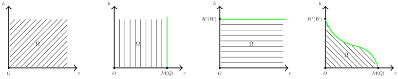
Figure 1: An illustration for the admissible domains $\Omega$ in different regimes, where the shadow region is the intersection of $\Omega$ and $(0,\infty)^{2}$. From left to right: D-D-regime, F-D-regime, D-F-regime and F-F-regime.

Remark 1.10.

By straightforward modification of the method developed in this paper, we are also able to give a new proof for the scattering result in the defocusing-defocusing regime using the concentration compactness principle. ∎

Outline of the paper

The paper is organized as follows: In Section 2 we establish the small data and stability theories for the (DCNLS). In Section 3 we construct the double track profile decomposition. Section 4 to Section 6 are devoted to the proof of Theorem 1.6, Proposition 1.8 and Proposition 1.9. In Appendix A we establish the endpoint values of the curve $c\mapsto m_{c}$ for the focusing-focusing (DCNLS).

1.1 Notations and definitions

We will use the notation $A\lesssim B$ whenever there exists some positive constant $C$ such that $A\leq CB$. Similarly we define $A\gtrsim B$ and we will use $A\sim B$ when $A\lesssim B\lesssim A$. We denote by $\|\cdot\|_{p}$ the $L^{p}(\mathbb{R}^{d})$-norm for $p\in[1,\infty]$. We similarly define the $H^{1}(\mathbb{R}^{d})$-norm by $\|\cdot\|_{H^{1}}$. The following quantities will be used throughout the paper:

$$\mathcal{M}(u) :=\|u\|^{2}_{2},$$

$$\mathcal{H}(u) :=\frac{1}{2}\|\nabla u\|_{2}^{2}-\frac{\mu_{1}}{{2_{*}}}\|u\|^{{2_{*}}}_{{2_{*}}}-\frac{\mu_{2}}{{2^{*}}}\|u\|^{{2^{*}}}_{{2^{*}}},$$

$$\mathcal{K}(u) :=\|\nabla u\|_{2}^{2}-\mu_{1}\frac{d}{d+2}\|u\|_{2_{*}}^{2_{*}}-\mu_{2}\|u\|_{2^{*}}^{2^{*}},$$

$$\mathcal{I}(u) :=\mathcal{H}(u)-\frac{1}{2}\mathcal{K}(u)=\frac{\mu_{2}}{d}\|u\|_{2^{*}}^{2^{*}}.$$

We will also frequently use the scaling operator

$$T_{\lambda}u(x) :=\lambda^{\frac{d}{2}}u(\lambda x).$$

One easily verifies that the $L^{2}$-norm is invariant under this scaling. Throughout the paper, we denote by $g_{\xi_{0},x_{0},\lambda_{0}}$ the $L^{2}$-symmetry transformation which is defined by

$$g_{\xi_{0},x_{0},\lambda_{0}}f(x):=\lambda_{0}^{-\frac{d}{2}}e^{i\xi_{0}\cdot x}f(\lambda_{0}^{-1}(x-x_{0}))$$

for $(\xi_{0},x_{0},\lambda_{0})\in\mathbb{R}^{d}\times\mathbb{R}^{d}\times(0,\infty)$.

We denote by $Q$ the unique positive and radially symmetric solution of

$$-\Delta Q+Q=Q^{{2_{*}}-1}.$$

We denote by $\mathrm{C}_{\mathrm{GN}}$ the optimal $L^{2}$-critical Gagliardo-Nirenberg constant, i.e.

$$\mathrm{C}_{\mathrm{GN}}=\inf_{u\in H^{1}(\mathbb{R}^{d})\setminus\{0\}}\frac{\|\nabla u\|_{2}^{2}\|u\|_{2}^{\frac{4}{d}}}{\|u\|_{{2_{*}}}^{{2_{*}}}}.$$ (1.12)

Using Pohozaev identities (see for instance [4]), the uniqueness of $Q$ and scaling arguments one easily verifies that

$$\mathrm{C}_{\mathrm{GN}}=\frac{d}{d+2}(\mathcal{M}(Q))^{\frac{2}{d}}.$$ (1.13)

We also denote by $\mathcal{S}$ the optimal constant for the Sobolev inequality, i.e.

$$\mathcal{S}:=\inf_{u\in\mathcal{D}^{1,2}(\mathbb{R}^{d})\setminus\{0\}}\frac{\|\nabla u\|_{2}^{2}}{\|u\|_{2^{*}}^{2}}.$$

Here, the space $\mathcal{D}^{1,2}(\mathbb{R}^{d})$ is defined by

$$\mathcal{D}^{1,2}(\mathbb{R}^{d}):=\{u\in L^{2^{*}}(\mathbb{R}^{d}):\nabla u\in L^{2}(\mathbb{R}^{d})\}.$$

For an interval $I\subset\mathbb{R}$, the space $L_{t}^{q}L_{x}^{r}(I)$ is defined by

$$L_{t}^{q}L_{x}^{r}(I):=\{u:I\times\mathbb{R}^{2}\to\mathbb{C}:\|u\|_{L_{t}^{q}L_{x}^{r}(I)}<\infty\},$$

where

$$\|u\|^{q}_{L_{t}^{q}L_{x}^{r}(I)}:=\int_{\mathbb{R}}\|u\|^{q}_{r}\,dt.$$

The following spaces will be frequently used throughout the paper:

$$S(I) :=L_{t}^{\infty}L_{x}^{2}(I)\cap L_{t}^{2}L_{x}^{{2^{*}}}(I),$$

$$V_{{2^{*}}}(I) :=L_{t}^{\frac{2(d+2)}{d-2}}L_{x}^{\frac{2d(d+2)}{d^{2}+4}}(I),$$

$$W_{{2^{*}}}(I) :=L_{t,x}^{\frac{2(d+2)}{d-2}}(I),$$

$$W_{{2_{*}}}(I) :=L_{t,x}^{\frac{2(d+2)}{d}}(I).$$

A pair $(q,r)$ is said to be $L^{2}$-admissible if $q,r\in[2,\infty]$, $\frac{2}{q}+\frac{d}{r}=\frac{d}{2}$ and $(q,r,d)\neq(2,\infty,2)$. For any $L^{2}$-admissible pairs $(q_{1},r_{1})$ and $(q_{2},r_{2})$ we have the following Strichartz estimates: if $u$ is a solution of

$$i\partial_{t}u+\Delta u=F(u)$$

in $I\subset\mathbb{R}$ with $t_{0}\in I$ and $u(t_{0})=u_{0}$, then

$$\|u\|_{L_{t}^{q}L_{x}^{r}(I)}\lesssim\|u_{0}\|_{2}+\|F(u)\|_{L_{t}^{q_{2}^{\prime}}L_{x}^{r_{2}^{\prime}}(I)},$$

where $(q_{2}^{\prime},r_{2}^{\prime})$ is the Hölder conjugate of $(q_{2},r_{2})$. For a proof, we refer to [25, 10].

In this paper, we use the following concepts for solution and scattering of (DCNLS):

Definiton 1.11 (Solution).

A function $u:I\times\mathbb{R}^{d}\to\mathbb{C}$ is said to be a solution of (DCNLS) on the interval $I\subset\mathbb{R}$ if for any compact $J\subset I$, $u\in C(J;H^{1}(\mathbb{R}^{d}))$ and for all $t,t_{0}\in I$

$$u(t)=e^{i(t-t_{0})\Delta}u(t_{0})+i\int_{t_{0}}^{t}e^{i(t-s)\Delta}[\mu_{1}|u|^{\frac{4}{d}}u+\mu_{2}|u|^{\frac{4}{d-2}}u](s)\,ds.$$

Definiton 1.12 (Scattering).

A global solution $u$ of (DCNLS) is said to be forward in time scattering if there exists some $\phi_{+}\in H^{1}(\mathbb{R}^{d})$ such that

$$\lim_{t\to\infty}\|u(t)-e^{it\Delta}\phi_{+}\|_{H^{1}}=0.$$

A backward in time scattering solution is similarly defined. $u$ is then called a scattering solution when it is both forward and backward in time scattering.

We define the Fourier transformation of a function $f$ by

$$\hat{f}(\xi)=\mathcal{F}(f)(\xi):=(2\pi)^{-\frac{d}{2}}\int_{\mathbb{R}^{d}}f(x)e^{-i\xi\cdot x}\,dx.$$

For $s\in\mathbb{R}$, the multipliers $|\nabla|^{s}$ and $\langle\nabla\rangle^{s}$ are defined by the symbols

$$|\nabla|^{s}f(x) =\mathcal{F}^{-1}\Big{(}|\xi|^{s}\hat{f}(\xi)\Big{)}(x),$$

$$\langle\nabla\rangle^{s}f(x) =\mathcal{F}^{-1}\Big{(}(1+|\xi|^{2})^{\frac{s}{2}}\hat{f}(\xi)\Big{)}(x).$$

Let $\psi\in C^{\infty}_{c}(\mathbb{R}^{2})$ be a fixed radial, non-negative and radially decreasing function such that $\psi(x)=1$ if $|x|\leq 1$ and $\psi(x)=0$ for $|x|\geq\frac{11}{10}$. Then for $N>0$, we define the Littlewood-Paley projectors by

$$P_{\leq N}f(x) =\mathcal{F}^{-1}\Big{(}\psi\Big{(}\frac{\xi}{N}\Big{)}\hat{f}(\xi)\Big{)}(x),$$

$$P_{N}f(x) =\mathcal{F}^{-1}\Big{(}\Big{(}\psi\Big{(}\frac{\xi}{N}\Big{)}-\psi\Big{(}\frac{2\xi}{N}\Big{)}\Big{)}\hat{f}(\xi)\Big{)}(x),$$

$$P_{>N}f(x) =\mathcal{F}^{-1}\Big{(}\Big{(}1-\psi\Big{(}\frac{\xi}{N}\Big{)}\Big{)}\hat{f}(\xi)\Big{)}(x).$$

We also record the following well-known Bernstein inequalities which will be frequently used throughout the paper: For all $s\geq 0$ and $1\leq p\leq q\leq\infty$ we have

$$\|P_{>N}f\|_{L^{p}} \lesssim N^{-s}\||\nabla|^{s}P_{>N}f\|_{L^{p}},$$

$$\||\nabla|^{s}P_{\leq N}f\|_{L^{p}} \lesssim N^{s}\|P_{\leq N}f\|_{L^{p}},$$

$$\||\nabla|^{\pm s}P_{N}f\|_{L^{p}} \sim N^{\pm s}\|P_{N}f\|_{L^{p}},$$

$$\|P_{\leq N}f\|_{L^{q}} \lesssim N^{\frac{n}{p}-\frac{n}{q}}\|P_{\leq N}f\|_{L^{p}},$$

$$\|P_{N}f\|_{L^{q}} \lesssim N^{\frac{n}{p}-\frac{n}{q}}\|P_{N}f\|_{L^{p}}.$$

The following useful elementary inequality will be frequently used in the paper: For $s\in\{0,1\}$ and $z_{1},\cdots,z_{k}\in\mathbb{C}$ we have

$$\Big{|}|\nabla|^{s}\Big{(}\Big{|}\sum_{j=1}^{k}z_{j}\Big{|}^{\alpha}\Big{(}\sum_{j=1}^{k}z_{j}\Big{)}-\sum_{j=1}^{k}|z_{j}|^{\alpha}z_{j}\Big{)}\Big{|}$$

$$\lesssim_{k,\alpha} \left\{\begin{array}[]{ll}\sum_{j\neq j^{\prime}}||\nabla|^{s}z_{j}||z_{j^{\prime}}|^{\alpha},&\text{if $0<\alpha\leq 1$},\\ \sum_{j\neq j^{\prime}}||\nabla|^{s}z_{j}||z_{j^{\prime}}|(|z_{j}|+|z_{j^{\prime}}|)^{\alpha-1},&\text{if $\alpha>1$}.\end{array}\right.$$ (1.16)

We end this section with the following useful local smoothing result:

Lemma 1.13 ([29]).

Given $\phi\in\dot{H}^{1}(\mathbb{R}^{d})$ we have

$$\|\nabla e^{it\Delta}\phi\|^{3}_{L_{t,x}^{2}([-T,T]\times\{|x|\leq R\})}\lesssim T^{\frac{2}{d+2}}R^{\frac{3d+2}{d+2}}\|e^{it\Delta}\phi\|_{W_{2^{*}}(\mathbb{R})}\|\nabla\phi\|^{2}_{2}.$$ (1.17)

2 Small data and stability theories

We record in this section the small data and stability theories for (DCNLS). The proof of the small data theory is standard, see for instance [10, 28]. We will therefore omit the details of the proof here.

Lemma 2.1 (Small data theory).

For any $A>0$ there exists some $\beta>0$ such that the following is true: Suppose that $t_{0}\in I$ for some interval $I$. Suppose also that $u_{0}\in H^{1}(\mathbb{R}^{d})$ with

$$\|u_{0}\|_{H^{1}}\leq A,$$ (2.1)

$$\|e^{i(t-t_{0})\Delta}u_{0}\|_{W_{{2_{*}}}\cap W_{{2^{*}}}(I)}\leq\beta.$$ (2.2)

Then (DCNLS) has a unique solution $u\in C(I;H^{1}(\mathbb{R}^{d}))$ with $u(t_{0})=u_{0}$ such that

$$\|\langle\nabla\rangle u\|_{S(I)} \lesssim\|u_{0}\|_{H^{1}},$$ (2.3)

$$\|u\|_{W_{{2_{*}}}\cap W_{{2^{*}}}(I)} \leq 2\|e^{i(t-t_{0})\Delta}u_{0}\|_{W_{{2_{*}}}\cap W_{{2^{*}}}(I)}.$$ (2.4)

By the uniqueness of the solution $u$ we can extend $I$ to some maximal open interval $I_{\max}=(T_{\min},T_{\max})$. We have the following blow-up criterion: If $T_{\max}<\infty$, then

$$\|u\|_{W_{{2_{*}}}\cap W_{2^{*}}([T,T_{\max}))}=\infty$$

for any $T\in I_{\max}$. A similar result holds for $T_{\min}>-\infty$. Moreover, if

$$\|u\|_{W_{{2_{*}}}\cap W_{2^{*}}(I_{\max})}<\infty,$$

then $I_{\max}=\mathbb{R}$ and $u$ scatters in time.

Remark 2.2.

Using Strichartz and Sobolev inequalities we infer that

$$\|e^{i(t-t_{0})\Delta}u_{0}\|_{W_{{2_{*}}}\cap W_{{2^{*}}}(I)}\lesssim\|u_{0}\|_{H^{1}}.$$

Thus Lemma 2.1 is applicable for all $u_{0}$ with sufficiently small $H^{1}$-norm. ∎

We will also need the following persistence of regularity result for (DCNLS).

Lemma 2.3 (Persistence of regularity for (DCNLS)).

Let $u$ be a solution of (DCNLS) on some interval $I$ with $t_{0}\in I$ and $\|u\|_{W_{2_{*}}\cap W_{2^{*}}(I)}<\infty$. Then

$$\||\nabla|^{s}u\|_{S(I)}\leq C(\|u\|_{W_{2_{*}}\cap W_{2^{*}}(I)},\||\nabla|^{s}u(t_{0})\|_{2}).$$ (2.5)

Proof.

We divide $I$ into $m$ subintervals $I_{1},I_{2},\cdots,I_{m}$ with $I_{j}=[t_{j-1},t_{j}]$ such that

$$\|u\|_{W_{2_{*}}\cap W_{2^{*}}(I_{j})}\leq\eta\ll 1.$$

for some small $\eta$ which is to be determined later. Then by Strichartz we have

$$\||\nabla|^{s}u\|_{S(I_{j})}\lesssim\||\nabla|^{s}u(t_{j})\|_{2}+(\eta^{\frac{4}{d}}+\eta^{\frac{4}{d-2}})\||\nabla|^{s}u\|_{S(I_{j})}.$$

Therefore choosing $\eta$ sufficiently small (where the smallness depends only on the Strichartz constants and is uniform for all subintervals $I_{j}$) and starting with $j=1$ we have

$$\||\nabla|^{s}u\|_{S(I_{1})}\leq C(\||\nabla|^{s}u(t_{0})\|_{2}).$$

In particular,

$$\||\nabla|^{s}u(t_{1})\|_{2}\leq C(\||\nabla|^{s}u(t_{0})\|_{2}).$$

Arguing inductively for all $j=2,\cdots,m-1$ and summing the estimates on all subintervals up yield the desired claim. ∎

Now we prove the stability theory for (DCNLS), which is a stronger version of the ones from [15, 32] under the enhanced condition (2.9).

Lemma 2.4 (Stability theory).

Let $d\geq 3$ and let $u\in C(I;H^{1}(\mathbb{R}^{d}))$ be a solution of (DCNLS) defined on some interval $I\ni t_{0}$. Assume also that $w\in C(I;H^{1}(\mathbb{R}^{d}))$ is an approximate solution of the following perturbed NLS

$$i\partial_{t}w+\Delta w+\mu_{1}|w|^{\frac{4}{d}}w+\mu_{2}|w|^{\frac{4}{d-2}}w+e=0$$ (2.6)

such that

$$\|u\|_{L_{t}^{\infty}H_{x}^{1}(I)} \leq B_{1},$$ (2.7)

$$\|w\|_{W_{2_{*}}\cap W_{2^{*}}(I)} \leq B_{2}$$ (2.8)

for some $B_{1},B_{2}>0$. Then there exists some positive $\beta_{0}=\beta_{0}(B_{1},B_{2})\ll 1$ with the following property: if

$$\|u(t_{0})-w(t_{0})\|_{H^{1}} \leq\beta,$$ (2.9)

$$\|\langle\nabla\rangle e\|_{L_{t,x}^{\frac{2(d+2)}{d+4}}(I)} \leq\beta$$ (2.10)

for some $0<\beta<\beta_{0}$, then

$$\|\langle\nabla\rangle(u-w)\|_{S(I)}\lesssim_{B_{1},B_{2}}\beta^{\kappa}.$$ (2.11)

for some $\kappa\in(0,1)$.

Proof.

From the results given in [15, 32] we already know that

$$\|u-w\|_{W_{2_{*}}\cap W_{2^{*}}(I)} \lesssim_{B_{1},B_{2}}\beta^{\kappa},$$

$$\|\langle\nabla\rangle u\|_{S(I)}+\|\langle\nabla\rangle w\|_{S(I)} \lesssim_{B_{1},B_{2}}1$$

for some $\kappa\in(0,1)$. We divide $I$ into $O\Big{(}\frac{C(B_{1},B_{2})}{\delta}\Big{)}$ intervals $I_{1},\cdots,I_{m}$ such that

$$\|u\|_{W_{2_{*}}\cap W_{2^{*}}(I_{j})}+\|w\|_{W_{2_{*}}\cap W_{2^{*}}(I_{j})}\leq\delta$$

for all $j=1,\cdots,m$, where $\delta>0$ is some small number to be determined. Denote $I_{1}=[t_{0},t_{1}]$. Using Hölder and (1.1) we infer that

$$\||\nabla|^{s}(|u|^{\frac{4}{d}}u-|w|^{\frac{4}{d}}w)\|_{L_{t,x}^{\frac{2(d+2)}{d+4}}(I_{1})}$$

$$\lesssim \left\{\begin{array}[]{ll}\|u-w\|_{W_{2_{*}}(I_{1})}(\|u\|^{\frac{4-d}{d}}_{W_{2_{*}}(I_{1})}+\|w\|^{\frac{4-d}{d}}_{W_{2_{*}}(I_{1})})\||\nabla|^{s}w\|_{W_{2_{*}}(I_{1})}\\ \quad+(\|v\|^{\frac{4}{d}}_{W_{2_{*}}(I_{1})}+\|w\|^{\frac{4}{d}}_{W_{2_{*}}(I_{1})})\||\nabla|^{s}(u-w)\|_{W_{2_{*}}(I_{1})},&\text{if $d=3$},\\ \\ (\|u\|^{\frac{4}{d}}_{W_{2_{*}}(I_{1})}+\|w\|^{\frac{4}{d}}_{W_{2_{*}}(I_{1})})\||\nabla|^{s}(u-w)\|_{W_{2_{*}}(I_{1})}\\ \quad+\|u-w\|^{\frac{4}{d}}_{W_{2_{*}}(I_{1})}(\||\nabla|^{s}u\|_{W_{2_{*}}(I_{1})}+\||\nabla|^{s}w\|_{W_{2_{*}}(I_{1})}),&\text{if $d\geq 4$},\\ \end{array}\right.$$ (2.17)

$$\||\nabla|^{s}(|u|^{\frac{4}{d-2}}u-|w|^{\frac{4}{d-2}}w)\|_{L_{t,x}^{\frac{2(d+2)}{d+4}}(I_{1})}$$

$$\lesssim \left\{\begin{array}[]{ll}\|u-w\|_{W_{2^{*}}(I_{1})}(\|u\|^{\frac{6-d}{d-2}}_{W_{2^{*}}(I_{1})}+\|w\|^{\frac{6-d}{d-2}}_{W_{2^{*}}(I_{1})})\||\nabla|^{s}w\|_{W_{2_{*}}(I_{1})}\\ \quad+(\|u\|^{\frac{4}{d-2}}_{W_{2^{*}}(I_{1})}+\|w\|^{\frac{4}{d-2}}_{W_{2^{*}}(I_{1})})\||\nabla|^{s}(u-w)\|_{W_{2_{*}}(I_{1})},&\text{if $d\leq 5$},\\ \\ (\|u\|^{\frac{4}{d-2}}_{W_{2^{*}}(I_{1})}+\|w\|^{\frac{4}{d-2}}_{W_{2^{*}}(I_{1})})\||\nabla|^{s}(u-w)\|_{W_{2_{*}}(I_{1})}\\ \quad+\|u-w\|^{\frac{4}{d-2}}_{W_{2^{*}}(I_{1})}(\||\nabla|^{s}u\|_{W_{2_{*}}(I_{1})}+\||\nabla|^{s}w\|_{W_{2_{*}}(I_{1})}),&\text{if $d\geq 6$}\\ \end{array}\right.$$ (2.23)

for $s\in\{0,1\}$. By Strichartz we also see that

$$\||\nabla|^{s}(u-w)\|_{S(I_{1})} \lesssim\||\nabla|^{s}(u(t_{0})-w(t_{0}))\|_{L^{2}}+\||\nabla|^{s}(|u|^{\frac{4}{d}}u-|w|^{\frac{4}{d}}w)\|_{L_{t,x}^{\frac{2(d+2)}{d+4}}(I_{1})}$$

$$\quad\quad+\||\nabla|^{s}(|u|^{\frac{4}{d-2}}u-|w|^{\frac{4}{d-2}}w)\|_{L_{t,x}^{\frac{2(d+2)}{d+4}}(I_{1})}+\||\nabla|^{s}e\|_{L_{t,x}^{\frac{2(d+2)}{d+4}}(I_{1})}.$$ (2.24)

Now we absorb the terms on the r.h.s. with $\|\nabla(u-w)\|_{W_{2_{*}}(I_{1})}$ to the l.h.s. (which is possible by choosing $\delta$ sufficiently small) to deduce that

$$\||\nabla|^{s}(u-w)\|_{S(I_{1})}\lesssim\beta^{\kappa}$$

for some (possibly smaller) $\kappa\in(0,1)$. In particular, we have

$$\|u(t_{1})-w(t_{1})\|_{H^{1}}\lesssim\beta^{\kappa}.$$

Therefore we can proceed with the previous arguments for all $I_{2},\cdots,I_{m}$ to conclude that

$$\||\nabla|^{s}(u-w)\|_{S(I_{j})}\lesssim\beta^{\kappa}$$

for all $j=1,\cdots,m$. The claim follows by summing the estimates on each subinterval up. ∎

3 Double track profile decomposition

In this section we construct the double track profile decomposition for a bounded sequence in $H^{1}(\mathbb{R}^{d})$. We begin with the following inverse Strichartz inequality along the $\dot{H}^{1}$-track, which is originally proved in [27] in the case $d=3$ and can be extended to arbitrary dimension $d\geq 3$ straightforwardly.

Lemma 3.1 (Inverse Strichartz inequality, $\dot{H}^{1}$-track, [27]).

Let $d\geq 3$ and $(f_{n})_{n}\subset H^{1}(\mathbb{R}^{d})$. Suppose that

$$\lim_{n\to\infty}\|f_{n}\|_{H^{1}}=A<\infty\quad\text{and}\quad\lim_{n\to\infty}\|e^{it\Delta}f_{n}\|_{W_{2^{*}}(\mathbb{R})}=\varepsilon>0.$$ (3.1)

Then up to a subsequence, there exist $\phi\in\dot{H}^{1}(\mathbb{R}^{d})$ and $(t_{n},x_{n},\lambda_{n})_{n}\subset\mathbb{R}\times\mathbb{R}^{d}\times(0,\infty)$ such that $\lambda_{n}\to\lambda_{\infty}\in[0,\infty)$, and if $\lambda_{\infty}>0$, then $\phi\in H^{1}(\mathbb{R}^{d})$. Moreover,

$$\lambda_{n}^{\frac{d}{2}-1}(e^{it_{n}\Delta}f_{n})(\lambda_{n}x+x_{n})\rightharpoonup\phi(x)\text{ weakly in }\left\{\begin{array}[]{ll}H^{1}(\mathbb{R}^{d}),&\text{if $\lambda_{\infty}>0$},\\ \dot{H}^{1}(\mathbb{R}^{d}),&\text{if $\lambda_{\infty}=0$}.\end{array}\right.$$ (3.4)

Setting

$$\phi_{n}:=\left\{\begin{array}[]{ll}\lambda_{n}^{-\frac{d}{2}-1}e^{-it_{n}\Delta}\Big{[}\phi(\frac{x-x_{n}}{\lambda_{n}})\Big{]},&\text{if $\lambda_{\infty}>0$},\\ \\ \lambda_{n}^{-\frac{d}{2}-1}e^{-it_{n}\Delta}\Big{[}(P_{>\lambda_{n}^{\theta}}\phi)(\frac{x-x_{n}}{\lambda_{n}})\Big{]},&\text{if $\lambda_{\infty}=0$}\end{array}\right.$$ (3.8)

for some fixed $\theta\in(0,1)$, we have

$$\lim_{n\to\infty}(\|f_{n}\|^{2}_{\dot{H}^{1}}-\|f_{n}-\phi_{n}\|^{2}_{\dot{H}^{1}})=\|\phi\|^{2}_{\dot{H}^{1}}\gtrsim A^{2}\Big{(}\frac{\varepsilon}{A}\Big{)}^{\frac{d(d+2)}{4}},$$ (3.9)

$$\lim_{n\to\infty}(\|f_{n}\|^{2}_{\dot{H}^{1}}-\|f_{n}-\phi_{n}\|^{2}_{\dot{H}^{1}}-\|\phi_{n}\|^{2}_{\dot{H}^{1}})=0,$$ (3.10)

$$\lim_{n\to\infty}(\|f_{n}\|^{2}_{2}-\|f_{n}-\phi_{n}\|^{2}_{2}-\|\phi_{n}\|^{2}_{2})=0.$$ (3.11)

Furthermore, we have

(i) $$\lambda_{n}\equiv 1\quad\text{or}\quad\lambda_{n}\to 0,$$ (3.12)

(ii) $$t_{n}\equiv 0\quad\text{or}\quad\frac{t_{n}}{\lambda_{n}^{2}}\to\pm\infty$$ (3.13)

and

$$\|f_{n}\|_{2_{*}}^{2_{*}}=\|\phi_{n}\|_{2_{*}}^{2_{*}}+\|f_{n}-\phi_{n}\|_{2_{*}}^{2_{*}}+o_{n}(1),$$ (3.14)

$$\|f_{n}\|_{2^{*}}^{2^{*}}=\|\phi_{n}\|_{2^{*}}^{2^{*}}+\|f_{n}-\phi_{n}\|_{2^{*}}^{2^{*}}+o_{n}(1).$$ (3.15)

Next, we establish the inverse Strichartz inequality along the $L^{2}$-track by using the arguments from the proof of Lemma 3.1 and from [28, 14]. For each $j\in{\mathbb{Z}}$, define $\mathcal{C}_{j}$ by

$$\mathcal{C}_{j}:=\Big{\{}\Pi_{i=1}^{d}[2^{j}k_{i},2^{j}(k_{i}+1))\subset\mathbb{R}^{d}:k\in{\mathbb{Z}}^{d}\Big{\}}$$

and $\mathcal{C}:=\cup_{j\in{\mathbb{Z}}}\,\mathcal{C}_{j}$. Given $Q\in\mathcal{C}$ we define $f_{Q}$ by $\hat{f}_{Q}:=\chi_{Q}\hat{f}$, where $\chi_{Q}$ is the characteristic function of the cube $Q$. We have the following improved Strichartz estimate:

Lemma 3.2 (Improved Strichartz estimate, [28]).

Let $d\geq 1$ and $q:=\frac{2(d^{2}+3d+1)}{d^{2}}$. Then

$$\|e^{it\Delta}f\|_{W_{2_{*}}(\mathbb{R})}\lesssim\|f\|_{2}^{\frac{d+1}{d+2}}\Big{(}\sup_{Q\in\mathcal{C}}|Q|^{\frac{d+2}{dq}-\frac{1}{2}}\|e^{it\Delta}f_{Q}\|_{L_{t,x}^{q}(\mathbb{R})}\Big{)}^{\frac{1}{d+2}}.$$ (3.16)

Lemma 3.3 (Inverse Strichartz inequality, $L^{2}$-track).

Let $d\geq 3$ and $(f_{n})_{n}\subset H^{1}(\mathbb{R}^{d})$. Suppose that

$$\lim_{n\to\infty}\|f_{n}\|_{H^{1}}=A<\infty\quad\text{and}\quad\lim_{n\to\infty}\|e^{it\Delta}f_{n}\|_{W_{2_{*}}(\mathbb{R})}=\varepsilon>0.$$ (3.17)

Then up to a subsequence, there exist $\phi\in L^{2}(\mathbb{R}^{d})$ and $(t_{n},x_{n},\xi_{n},\lambda_{n})_{n}\subset\mathbb{R}\times\mathbb{R}^{d}\times\mathbb{R}^{d}\times(0,\infty)$ such that $\limsup_{m\to\infty}|\xi_{n}|<\infty$ and $\lim_{n\to\infty}\lambda_{n}=:\lambda_{\infty}\in(0,\infty]$. Moreover,

$$\,\,\lambda_{n}^{\frac{d}{2}}e^{-i\xi_{n}\cdot(\lambda_{n}x+x_{n})}(e^{it_{n}\Delta}f_{n})(\lambda_{n}x+x_{n})$$

$$\rightharpoonup \,\,\phi(x)\text{ weakly in }\left\{\begin{array}[]{ll}H^{1}(\mathbb{R}^{d}),&\text{if $\limsup_{n\to\infty}|\lambda_{n}\xi_{n}|<\infty$},\\ L^{2}(\mathbb{R}^{d}),&\text{if $|\lambda_{n}\xi_{n}|\to\infty$}.\end{array}\right.$$ (3.20)

Addtionally, if $\limsup_{n\to\infty}|\lambda_{n}\xi_{n}|<\infty$, then $\xi_{n}\equiv 0$. Setting

$$\phi_{n}:=\left\{\begin{array}[]{ll}\lambda_{n}^{-\frac{d}{2}}e^{-it_{n}\Delta}\Big{[}\phi(\frac{x-x_{n}}{\lambda_{n}})\Big{]},&\text{if $\lambda_{\infty}<\infty$},\\ \\ \lambda_{n}^{-\frac{d}{2}}e^{-it_{n}\Delta}\Big{[}e^{i\xi_{n}\cdot x}(P_{\leq\lambda_{n}^{\theta}}\phi)(\frac{x-x_{n}}{\lambda_{n}})\Big{]},&\text{if $\lambda_{\infty}=\infty$}\end{array}\right.$$ (3.24)

for some fixed $\theta\in(0,1)$, we have

$$\lim_{n\to\infty}(\|f_{n}\|^{2}_{2}-\|f_{n}-\phi_{n}\|^{2}_{2})=\|\phi\|^{2}_{2}\gtrsim A^{2}\Big{(}\frac{\varepsilon}{A}\Big{)}^{2(d+1)(d+2)},$$ (3.25)

$$\lim_{n\to\infty}(\|f_{n}\|^{2}_{\dot{H}^{1}}-\|f_{n}-\phi_{n}\|^{2}_{\dot{H}^{1}}-\|\phi_{n}\|^{2}_{\dot{H}^{1}})=0,$$ (3.26)

$$\lim_{n\to\infty}(\|f_{n}\|^{2}_{2}-\|f_{n}-\phi_{n}\|^{2}_{2}-\|\phi_{n}\|^{2}_{2})=0.$$ (3.27)

Proof.

For $R>0$, denote by $f^{R}$ the function such that $\mathcal{F}(f^{R})=\chi_{R}\hat{f}$, where $\chi_{R}$ is the characteristic function of the ball $B_{R}(0)$. First we obtain that

$$\sup_{n\in\mathbb{N}}\|f_{n}-f_{n}^{R}\|_{2}^{2}=\sup_{n\in\mathbb{N}}\int_{|\xi|\geq R}|\hat{f}_{n}(\xi)|^{2}\,d\xi\leq R^{-2}\sup_{n\in\mathbb{N}}\|f_{n}\|_{\dot{H}^{1}}^{2}\lesssim R^{-2}A^{2}\to 0$$ (3.28)

as $R\to\infty$. Combining with Strichartz, we infer that there exists some $K_{1}>0$ such that for all $R\geq K_{1}$ one has

$$\sup_{n\in\mathbb{N}}\|f^{R}_{n}\|_{2}\lesssim A\quad\text{and}\quad\sup_{n\in\mathbb{N}}\|e^{it\Delta}f^{R}_{n}\|_{W_{2_{*}}(\mathbb{R})}\gtrsim\varepsilon.$$

Applying Lemma 3.2 to $(f^{R}_{n})_{n}$, we know that there exists $(Q_{n})_{n}\subset\mathcal{C}$ such that

$$\varepsilon^{d+2}A^{-(d+1)}\lesssim\inf_{n\in\mathbb{N}}|Q_{n}|^{\frac{d+2}{dq}-\frac{1}{2}}\|e^{it\Delta}(f^{R}_{n})_{Q_{n}}\|_{L^{q}_{t,x}(\mathbb{R})}.$$ (3.29)

Let $\lambda_{n}^{-1}$ be the side-length of $Q_{n}$. Denote also by $\xi_{n}$ the center of $Q_{n}$. Since $q\in(\frac{2(d+2)}{d},\frac{2(d+2)}{d-2})$ for $d\geq 3$, using Hölder and Strichartz we obtain that

$$\sup_{n\in\mathbb{N}}\|e^{it\Delta}(f^{R}_{n})_{Q_{n}}\|_{L^{q}_{t,x}(\mathbb{R})}\lesssim\sup_{n\in\mathbb{N}}\|f_{n}\|_{H^{1}}\lesssim A.$$

Combining with the fact that $\frac{d+2}{dq}-\frac{1}{2}<0$, we deduce that $\sup_{n\in\mathbb{N}}|Q_{n}|\lesssim 1$. Since $(\mathcal{F}(f_{n}^{R}))_{n}$ are supported in $B_{R}(0)$, we may assume that $(Q_{n})_{n}\subset B_{R^{\prime}}(0)$ for some sufficiently large $R^{\prime}>0$. Therefore $(\lambda_{n})_{n}$ is bounded below and $(\xi_{n})_{n}$ is bounded in $\mathbb{R}^{d}$. Hölder yields

$$|Q_{n}|^{\frac{d+2}{dq}-\frac{1}{2}}\|e^{it\Delta}(f^{R}_{n})_{Q_{n}}\|_{L^{q}_{t,x}(\mathbb{R})} \lesssim\lambda_{n}^{\frac{d}{2}-\frac{d+2}{q}}\|e^{it\Delta}(f^{R}_{n})_{Q_{n}}\|^{\frac{d(d+2)}{d^{2}+3d+1}}_{W_{2_{*}}(\mathbb{R})}\|e^{it\Delta}(f^{R}_{n})_{Q_{n}}\|^{\frac{d+1}{d^{2}+3d+1}}_{L_{t,x}^{\infty}(\mathbb{R})}$$

$$\lesssim\lambda_{n}^{\frac{d}{2}-\frac{d+2}{q}}\varepsilon^{\frac{d(d+2)}{d^{2}+3d+1}}\|e^{it\Delta}(f^{R}_{n})_{Q_{n}}\|^{\frac{d+1}{d^{2}+3d+1}}_{L_{t,x}^{\infty}(\mathbb{R})}.$$

Combining with (3.29) we infer that there exist $(t_{n},x_{n})_{n}\subset\mathbb{R}\times\mathbb{R}^{d}$ such that

$$\liminf_{n\to\infty}\lambda_{n}^{\frac{d}{2}}|[e^{it_{n}\Delta}(f^{R}_{n})_{Q_{n}}](x_{n})|\gtrsim\varepsilon^{(d+1)(d+2)}A^{-(d^{2}+3d+1)}.$$ (3.30)

Define

$$h_{n}(x) :=\lambda_{n}^{\frac{d}{2}}e^{-i\xi_{n}(\lambda_{n}x+x_{n})}(e^{it_{n}\Delta}f_{n})(\lambda_{n}x+x_{n}),$$

$$h^{R}_{n}(x) :=\lambda_{n}^{\frac{d}{2}}e^{-i\xi_{n}(\lambda_{n}x+x_{n})}(e^{it_{n}\Delta}f^{R}_{n})(\lambda_{n}x+x_{n}).$$

It is easy to verify that $\|h_{n}\|_{2}=\|f_{n}\|_{2}$. By the $L^{2}$-boundedness of $(f_{n})_{n}$ we know that there exists some $\phi\in L^{2}(\mathbb{R}^{d})$ such that $h_{n}\rightharpoonup\phi$ weakly in $L^{2}(\mathbb{R}^{d})$. Arguing similarly, we infer that $(h^{R}_{n})_{n}$ converges weakly to some $\phi^{R}\in L^{2}(\mathbb{R}^{d})$. By definition of $\phi$ and $\phi^{R}$ we see that

$$\|\phi-\phi^{R}\|^{2}_{2}=\lim_{n\to\infty}\langle h_{n}-h_{n}^{R},\phi-\phi^{R}\rangle_{L^{2}}\leq(\limsup_{n\to\infty}\|h_{n}-h_{n}^{R}\|_{2})\|\phi-\phi^{R}\|_{2}.$$

Using (3.28) we then obtain that

$$\phi^{R}\to\phi\quad\text{in $L^{2}(\mathbb{R}^{d})$ as $R\to\infty$}.$$ (3.31)

Now define the function $\chi$ such that $\hat{\chi}$ is the characteristic function of the cube $[-\frac{1}{2},\frac{1}{2})^{d}$. From (3.30), the weak convergence of $h^{R}_{n}$ to $\phi^{R}$ in $L^{2}(\mathbb{R}^{d})$ and change of variables it follows

$$\langle\phi^{R},\chi\rangle=\lim_{n\to\infty}\lambda_{n}^{\frac{d}{2}}|[e^{it_{n}\Delta}(f^{R}_{n})_{Q_{n}}](x_{n})|\gtrsim\varepsilon^{(d+1)(d+2)}A^{-(d^{2}+3d+1)}.$$ (3.32)

On the other hand, using Hölder we also have

$$|\langle\phi^{R},\chi\rangle|\leq\|\phi^{R}\|_{2}\|\chi\|_{2}.$$

Thus

$$\|\phi^{R}\|_{2}^{2}\geq C\varepsilon^{2(d+1)(d+2)}A^{-2(d^{2}+3d+1)}$$ (3.33)

for some $C=C(d)>0$ which is uniform for all $R\geq K_{1}$. Now using (3.31) and (3.33) we finally deduce that

$$\|\phi\|_{2}^{2}\geq\|\phi^{R}\|_{2}^{2}-\frac{C}{2}\varepsilon^{2(d+1)(d+2)}A^{-2(d^{2}+3d+1)}\geq\frac{C}{2}\varepsilon^{2(d+1)(d+2)}A^{-2(d^{2}+3d+1)}$$ (3.34)

for sufficiently large $R$, which gives the lower bound of (3.25). From now on we fix $R$ such that the lower bound of (3.25) is valid for this chosen $R$ and let $(t_{n},x_{n},\xi_{n},\lambda_{n})_{n}$ be the corresponding symmetry parameters. Since $L^{2}(\mathbb{R}^{d})$ is a Hilbert space, from the weak convergence of $h_{n}$ to $\phi$ in $L^{2}(\mathbb{R}^{d})$ we obtain that

$$\lim_{n\to\infty}(\|h_{n}\|^{2}_{2}-\|\phi\|^{2}_{2}-\|h_{n}-\phi\|^{2}_{2})=2\lim_{n\to\infty}\mathrm{Re}\,\langle\phi,h_{n}-\phi\rangle_{L^{2}}=0.$$

Combining with the fact that

$$\|P_{\leq\lambda_{n}^{\theta}}\phi-\phi\|_{2}\to 0\quad\text{as $n\to\infty$}$$

for $\lambda_{n}\to\infty$ we conclude the equalities of (3.25) and (3.27). In the case $\limsup_{n\to\infty}|\lambda_{n}\xi_{n}|<\infty$, using the boundedness of $(\lambda_{n}\xi_{n})_{n}$ and chain rule, we also infer that $\|h_{n}\|_{H^{1}}\lesssim\|f_{n}\|_{H^{1}}$. By the $H^{1}$-boundedness of $(f_{n})_{n}$ and uniqueness of weak convergence we deduce additionally that $\phi\in H^{1}(\mathbb{R}^{d})$ and (3.3) follows.

Next we show that we may assume $\xi_{n}\equiv 0$ under the additional condition $\limsup_{n\to\infty}|\lambda_{n}\xi_{n}|<\infty$. Define

$$\mathcal{T}_{a,b}u(x):=be^{ia\cdot x}u(x)$$

for $a\in\mathbb{R}^{d}$ and $b\in\mathbb{C}$ with $|b|=1$. Let also

$$(\lambda\xi)_{\infty} :=\lim_{n\to\infty}\lambda_{n}\xi_{n},$$

$$e^{i(\xi\cdot x)_{\infty}} :=\lim_{n\to\infty}e^{i\xi_{n}\cdot x_{n}}.$$

By the boundedness of $(\lambda_{n}\xi_{n})_{n}$ we infer that $\mathcal{T}_{\lambda_{n}\xi_{n},e^{i\xi_{n}\cdot x_{n}}}$ is an isometry on $L^{2}(\mathbb{R}^{d})$ and converges strongly to $\mathcal{T}_{(\lambda\xi)_{\infty},e^{i(\xi\cdot x)_{\infty}}}$ as operators on $H^{1}(\mathbb{R}^{d})$. We may replace $h_{n}$ by $\lambda_{n}^{\frac{d}{2}}(e^{it_{n}\Delta}f_{n})(\lambda_{n}x+x_{n})$ and $\phi$ by $\mathcal{T}_{(\lambda\xi)_{\infty},e^{i(\xi\cdot x)_{\infty}}}\phi$ and (3.3), (3.25) and (3.26) carry over.

Finally, we prove (3.26). For the case $\lambda_{\infty}<\infty$ we additionally know that $\phi\in H^{1}(\mathbb{R}^{d})$ and $\xi_{n}\equiv 0$. Using the fact that $\dot{H}^{1}$ is a Hilbert space and change of variables we obtain that

$$o_{n}(1)=\|h_{n}\|_{\dot{H^{1}}}-\|h_{n}-\phi\|_{\dot{H^{1}}}-\|\phi\|_{\dot{H^{1}}}=\lambda_{n}^{2}(\|f_{n}\|_{\dot{H^{1}}}-\|f_{n}-\phi_{n}\|_{\dot{H^{1}}}-\|\phi_{n}\|_{\dot{H^{1}}}).$$

Combining with the lower boundedness of $(\lambda_{n})_{n}$, this implies that

$$\|f_{n}\|_{\dot{H^{1}}}-\|f_{n}-\phi_{n}\|_{\dot{H^{1}}}-\|\phi_{n}\|_{\dot{H^{1}}}=\lambda_{n}^{-2}o_{n}(1)=o_{n}(1),$$

which gives (3.26) in the case $\lambda_{\infty}<\infty$. Assume now $\lambda_{\infty}=\infty$. Using change of variables and chain rule we obtain that

$$\,\|f_{n}\|^{2}_{\dot{H}^{1}}-\|f_{n}-\phi_{n}\|^{2}_{\dot{H}^{1}}-\|\phi_{n}\|^{2}_{\dot{H}^{1}}$$

$$= \,|\xi_{n}|^{2}\Big{(}\|h_{n}\|_{2}^{2}-\|h_{n}-P_{\leq\lambda_{n}^{\theta}}\phi\|^{2}_{2}-\|P_{\leq\lambda_{n}^{\theta}}\phi\|^{2}_{2}\Big{)}$$

$$+2\lambda_{n}^{-1}\mathrm{Re}\Big{(}\langle i\xi_{n}(h_{n}-P_{\leq\lambda_{n}^{\theta}}\phi),\nabla P_{\leq\lambda_{n}^{\theta}}\phi\rangle+\langle i\xi_{n}P_{\leq\lambda_{n}^{\theta}}\phi,\nabla(h_{n}-P_{\leq\lambda_{n}^{\theta}}\phi)\rangle\Big{)}$$

$$+\lambda_{n}^{-2}\Big{(}\|h_{n}\|^{2}_{\dot{H}^{1}}-\|h_{n}-P_{\leq\lambda_{n}^{\theta}}\phi\|^{2}_{\dot{H}^{1}}-\|P_{\leq\lambda_{n}^{\theta}}\phi\|^{2}_{\dot{H}^{1}}\Big{)}$$

$$=: \,I_{1}+I_{2}+I_{3}.$$ (3.35)

Using the boundedness of $(\xi_{n})_{n}$ and (3.27) we infer that $I_{1}\to 0$. For $I_{2}$, using Bernstein and the boundedness of $(\xi_{n})_{n}$ in $\mathbb{R}^{d}$ and of $(h_{n}-P_{\leq\lambda_{n}^{\theta}}\phi)$ in $L^{2}(\mathbb{R}^{d})$ we see that

$$|I_{2}|\lesssim\lambda_{n}^{-1}\|h_{n}-P_{\leq\lambda_{n}^{\theta}}\phi\|_{2}\|\nabla P_{\leq\lambda_{n}^{\theta}}\phi\|_{2}\lesssim\lambda_{n}^{-(1-\theta)}\to 0.$$

Finally, $I_{3}$ can be similarly estimated using Bernstein inequality, we omit the details here. Summing up we conclude (3.27). ∎

Lemma 3.4.

We have

(i) $$\lambda_{n}\equiv 1\quad\text{or}\quad\lambda_{n}\to\infty,$$ (3.36)

(ii) $$t_{n}\equiv 0\quad\text{or}\quad\frac{t_{n}}{\lambda_{n}^{2}}\to\pm\infty.$$ (3.37)

Proof.

If $\lambda_{n}\to\infty$, then there is nothing to prove. Otherwise assume that $\lambda_{\infty}<\infty$. By the boundedness of $(\xi_{n})_{n}$ we also know that $\phi\in H^{1}(\mathbb{R}^{d})$ and $(\lambda_{n}\xi_{n})_{n}$ is bounded, thus $\xi_{n}\equiv 0$ and $h_{n}(x)$ reduces to $\lambda_{n}^{\frac{d}{2}}(e^{it_{n}\Delta}f_{n})(\lambda_{n}x+x_{n})$. Define

$$\mathcal{J}_{\lambda}f(x):=\lambda^{-\frac{d}{2}}f(\lambda^{-1}x).$$

Then $\mathcal{J}_{\lambda_{n}}$ and $\mathcal{J}^{-1}_{\lambda_{n}}$ converge strongly to $\mathcal{J}_{\lambda_{\infty}}$ and $\mathcal{J}^{-1}_{\lambda_{\infty}}$ strongly as operators in $H^{1}(\mathbb{R}^{d})$. We may redefine $\lambda_{n}\equiv 1$ and replace $\phi$ by $\mathcal{J}_{\lambda_{\infty}}\phi$, and all the statements from Lemma 3.3 continue to hold.

We now prove (ii). If $\frac{t_{n}}{\lambda_{n}^{2}}\to\pm\infty$, then we are done. Otherwise assume that $\frac{t_{n}}{\lambda_{n}^{2}}\to\tau_{\infty}\in\mathbb{R}$. Recall that for $(\xi_{0},x_{0},\lambda_{0})\in\mathbb{R}^{d}\times\mathbb{R}^{d}\times(0,\infty)$ the operator $g_{\xi_{0},x_{0},\lambda_{0}}$ is defined by

$$g_{\xi_{0},x_{0},\lambda_{0}}f(x)=\lambda_{0}^{-\frac{d}{2}}e^{i\xi_{0}\cdot x}f(\lambda_{0}^{-1}(x-x_{0})).$$

Then

$$f_{n}=e^{-it_{n}\Delta}[g_{\xi_{n},x_{n},\lambda_{n}}h_{n}](x)$$

and

$$\phi_{n}=\left\{\begin{array}[]{ll}e^{-it_{n}\Delta}[g_{\xi_{n},x_{n},\lambda_{n}}\phi](x),&\text{if $\lambda_{\infty}<\infty$},\\ \\ e^{-it_{n}\Delta}[g_{\xi_{n},x_{n},\lambda_{n}}P_{\leq\lambda_{n}^{\theta}}\phi](x),&\text{if $\lambda_{\infty}=\infty$}.\end{array}\right.$$

Using the invariance of the NLS-flow under the Galilean transformation we infer that

$$e^{-it_{n}\Delta}[g_{\xi_{n},x_{n},\lambda_{n}}f](x)=g_{\xi_{n},x_{n}-2t_{n}\xi_{n},\lambda_{n}}[e^{it_{n}|\xi_{n}|^{2}}e^{-i\frac{t_{n}}{\lambda_{n}^{2}}\Delta}f](x).$$ (3.38)

Denote $\beta:=\lim_{n\to\infty}e^{it_{n}|\xi_{n}|^{2}}$. We can therefore redefine $t_{n}$ by $0$, $x_{n}$ by $x_{n}-2t_{n}\xi_{n}$ and $\phi$ by $\beta e^{-i\tau_{\infty}\Delta}\phi$. One easily checks that up to (3.26) in the case $\lambda_{\infty}=\infty$, the statements from Lemma 3.3 carry over, due to the strong continuity of the linear Schrödinger flow on $H^{1}(\mathbb{R}^{d})$ and the fact that $g$ is an isometry on $L^{2}(\mathbb{R}^{d})$. To see (3.26) in the case $\lambda_{\infty}=\infty$, we obtain that

$$\|g_{\xi_{n},x_{n}-2t_{n}\xi_{n},\lambda_{n}}[e^{it_{n}|\xi_{n}|^{2}}e^{-i\frac{t_{n}}{\lambda_{n}^{2}}\Delta}P_{\leq\lambda_{n}^{\theta}}\phi]-g_{\xi_{n},x_{n}-2t_{n}\xi_{n},\lambda_{n}}[\beta e^{-i\tau_{\infty}\Delta}P_{\leq\lambda_{n}^{\theta}}\phi]\|_{\dot{H}^{1}}$$

$$\lesssim \,|\xi_{n}|\|e^{it_{n}|\xi_{n}|^{2}}e^{-i\frac{t_{n}}{\lambda_{n}^{2}}\Delta}P_{\leq\lambda_{n}^{\theta}}\phi-\beta e^{-i\tau_{\infty}\Delta}P_{\leq\lambda_{n}^{\theta}}\phi\|_{2}$$

$$+\lambda_{n}^{-1}\|e^{it_{n}|\xi_{n}|^{2}}e^{-i\frac{t_{n}}{\lambda_{n}^{2}}\Delta}P_{\leq\lambda_{n}^{\theta}}\phi-\beta e^{-i\tau_{\infty}\Delta}P_{\leq\lambda_{n}^{\theta}}\phi\|_{\dot{H}^{1}}=:I_{1}+I_{2}.$$ (3.39)

By the boundedness of $(\xi_{n})_{n}$ one easily verifies that $I_{1}\to 0$. Using Bernstein we see that

$$|I_{2}|\lesssim\lambda_{n}^{-(1-\theta)}\|P_{\leq\lambda_{n}^{\theta}}\phi\|_{2}\lesssim\lambda^{-(1-\theta)}_{n}\|\phi\|_{2}\to 0.$$ (3.40)

This completes the desired proof. ∎

Remark 3.5.

Using (3.38), redefining the parameters and taking Lemma 3.1 into account we may assume that

$$\phi_{n}=\left\{\begin{array}[]{ll}\lambda_{n}g_{0,x_{n},\lambda_{n}}[e^{it_{n}\Delta}P_{>\lambda_{n}^{\theta}}\phi](x),&\text{if $\lambda_{\infty}=0$},\\ \\ e^{it_{n}\Delta}\phi(x-x_{n}),&\text{if $\lambda_{\infty}=1$},\\ \\ g_{\xi_{n},x_{n},\lambda_{n}}[e^{it_{n}\Delta}P_{\leq\lambda_{n}^{\theta}}\phi](x),&\text{if $\lambda_{\infty}=\infty$}.\end{array}\right.$$

∎

Lemma 3.6.

We have

$$\|f_{n}\|_{2_{*}}^{2_{*}}=\|\phi_{n}\|_{2_{*}}^{2_{*}}+\|f_{n}-\phi_{n}\|_{2_{*}}^{2_{*}}+o_{n}(1),$$ (3.41)

$$\|f_{n}\|_{2^{*}}^{2^{*}}=\|\phi_{n}\|_{2^{*}}^{2^{*}}+\|f_{n}-\phi_{n}\|_{2^{*}}^{2^{*}}+o_{n}(1).$$ (3.42)

Proof.

Assume first that $\lambda_{\infty}=\infty$. Using Bernstein and Sobolev we infer that

$$\|\phi_{n}\|_{2^{*}}=\lambda^{-1}_{n}\|P_{\leq\lambda_{n}^{\theta}}\phi\|_{\dot{H}^{1}}\lesssim\lambda^{-(1-\theta)}_{n}\|\phi\|_{2}\to 0.$$

Hence $\|\phi_{n}\|_{2^{*}}=o_{n}(1)$. Therefore by triangular inequality

$$\Big{|}\|f_{n}\|_{2^{*}}-\|f_{n}-\phi_{n}\|_{2^{*}}\Big{|}\leq\|\phi_{n}\|_{2^{*}}\to 0$$

and (3.42) follows. Now suppose that $\lambda_{\infty}=1$ and $t_{n}\to\pm\infty$. For $\beta>0$ let $\psi\in\mathcal{S}(\mathbb{R}^{d})$ such that

$$\|\phi-\psi\|_{H^{1}}\leq\beta.$$

Define

$$\psi_{n}:=e^{it_{n}\Delta}\psi(x-x_{n}).$$

Then by dispersive estimate we deduce that

$$\|\psi_{n}\|_{{2^{*}}}\lesssim|t_{n}|^{-1}\|\psi\|_{({2^{*}})^{\prime}}\to 0.$$

On the other hand, by Sobolev we have

$$\|\psi_{n}-\phi_{n}\|_{2^{*}}\lesssim\|\psi-\phi\|_{\dot{H}^{1}}\leq\beta.$$

Hence $\|\psi_{n}\|_{2^{*}}\lesssim\beta$ for all sufficiently large $n$. Therefore by triangular inequality

$$\Big{|}\|f_{n}\|_{2^{*}}-\|f_{n}-\psi_{n}\|_{2^{*}}\Big{|}\lesssim\beta$$

and (3.42) follows by taking $\beta$ arbitrarily small. Now we assume $\lambda_{\infty}=1$ and $t_{n}\equiv 0$. Then we additionally know that $\phi\in H^{1}(\mathbb{R}^{d})$ and $h_{n}\rightharpoonup\phi$ in $H^{1}(\mathbb{R}^{d})$. Using the Brezis-Lieb lemma we deduce that

$$\|h_{n}\|_{2^{*}}^{2^{*}}=\|\phi\|_{2^{*}}^{2^{*}}+\|h_{n}-\phi\|_{2^{*}}^{2^{*}}+o_{n}(1).$$

Undoing the transformation we obtain (3.42).

We now consider (3.41). When $\lambda_{\infty}=\infty$ or $\lambda_{\infty}=1$ and $t_{n}\to\pm\infty$, then $\|\psi_{n}\|_{2^{*}}\to 0$, and by Hölder we will also have $\|\psi_{n}\|_{2_{*}}\to 0$, thus (3.41) follows. For the case $\lambda_{\infty}=1$ and $t_{n}\equiv 0$, (3.41) follows again from the Brezis-Lieb lemma. This completes the desired proof. ∎

Having all the preliminaries we are in the position to establish the double track profile decomposition.

Lemma 3.7 (Double track profile decomposition).

Let $(\psi_{n})_{n}$ be a bounded sequence in $H^{1}(\mathbb{R}^{d})$. Then up to a subsequence, there exist nonzero linear profiles $({\phi}^{j})_{j}\subset\dot{H}^{1}(\mathbb{R}^{d})\cup L^{2}(\mathbb{R}^{d})$, remainders $(w_{n}^{k})_{k,n}\subset H^{1}(\mathbb{R}^{d})$, parameters $(t^{j}_{n},x^{j}_{n},\xi^{j}_{n},\lambda^{j}_{n})_{j,n}\subset\mathbb{R}\times\mathbb{R}^{d}\times\mathbb{R}^{d}\times(0,\infty)$ and $K^{*}\in\mathbb{N}\cup\{\infty\}$, such that

• For any finite $1\leq j\leq K^{*}$ the parameters satisfy

  $$1 \gtrsim_{j}\lim_{n\to\infty}|\xi_{n}^{j}|,$$

  $$\lim_{n\to\infty}\lambda^{j}_{n} =:t_{\infty}^{j}\in\{0,\pm\infty\},$$

  $$\lim_{n\to\infty}\lambda^{j}_{n} =:\lambda_{\infty}^{j}\in\{0,1,\infty\},$$

  $$t_{n}^{j} \equiv 0\quad\text{if $t_{\infty}^{j}=0$},$$

  $$\lambda_{n}^{j} \equiv 1\quad\text{if $\lambda_{\infty}^{j}=1$},$$

  $$\xi_{n}^{j} \equiv 0\quad\text{if $\lambda_{\infty}^{j}\in\{0,1\}$}.$$ (3.43)

• For any finite $1\leq k\leq K^{*}$ we have the decomposition

  $$\psi_{n}=\sum_{j=1}^{k}T^{j}_{n}P_{n}^{j}{\phi}^{j}+w_{n}^{k}.$$ (3.44)

  Here, the operators $T_{n}^{j}$ and $P_{n}^{j}$ are defined by

  $$T^{j}_{n}u(x):=\left\{\begin{array}[]{ll}\lambda^{j}_{n}g_{0,x^{j}_{n},\lambda^{j}_{n}}[e^{it^{j}_{n}\Delta}u](x),&\text{if $\lambda^{j}_{\infty}=0$},\\ \\ \,\,[e^{it^{j}_{n}\Delta}u](x-x^{j}_{n}),&\text{if $\lambda^{j}_{\infty}=1$},\\ \\ g_{\xi^{j}_{n},x^{j}_{n},\lambda^{j}_{n}}[e^{it^{j}_{n}\Delta}u](x),&\text{if $\lambda^{j}_{\infty}=\infty$}\end{array}\right.$$ (3.50)

  and

  $$P^{j}_{n}u:=\left\{\begin{array}[]{ll}P_{>(\lambda_{n}^{j})^{\theta}}u,&\text{if $\lambda^{j}_{\infty}=0$},\\ \\ u,&\text{if $\lambda^{j}_{\infty}=1$},\\ \\ P_{\leq(\lambda_{n}^{j})^{\theta}}u,&\text{if $\lambda^{j}_{\infty}=\infty$}\end{array}\right.$$ (3.56)

  for some $\theta\in(0,1)$. Moreover,

  $${\phi}^{j}\in\left\{\begin{array}[]{ll}\dot{H}^{1}(\mathbb{R}^{d}),&\text{if $\lambda^{j}_{\infty}=0$},\\ \\ H^{1}(\mathbb{R}^{d}),&\text{if $\lambda^{j}_{\infty}=1$},\\ \\ L^{2}(\mathbb{R}^{d}),&\text{if $\lambda^{j}_{\infty}=\infty$}.\end{array}\right.$$ (3.62)

• The remainders $(w_{n}^{k})_{k,n}$ satisfy

  $$\lim_{k\to K^{*}}\lim_{n\to\infty}\|e^{it\Delta}w_{n}^{k}\|_{W_{2_{*}}\cap W_{2^{*}}(\mathbb{R})}=0.$$ (3.63)

• The parameters are orthogonal in the sense that

  $$\frac{\lambda_{n}^{k}}{\lambda_{n}^{j}}+\frac{\lambda_{n}^{j}}{\lambda_{n}^{k}}+\lambda_{n}^{k}|\xi_{n}^{j}-\xi_{n}^{k}|+\Big{|}t_{k}\Big{(}\frac{\lambda_{n}^{k}}{\lambda_{n}^{j}}\Big{)}^{2}-t_{n}^{j}\Big{|}+\Big{|}\frac{x_{n}^{j}-x_{n}^{k}-2t_{n}^{k}(\lambda_{n}^{k})^{2}(\xi_{n}^{j}-\xi_{n}^{k})}{\lambda_{n}^{k}}\Big{|}\to\infty$$ (3.64)

  for any $j\neq k$.

• For any finite $1\leq k\leq K^{*}$ we have the energy decompositions

  $$\||\nabla|^{s}\psi_{n}\|_{2}^{2} =\sum_{j=1}^{k}\||\nabla|^{s}T_{n}^{j}P_{n}^{j}{\phi}^{j}\|_{2}^{2}+\||\nabla|^{s}w_{n}^{k}\|_{2}^{2}+o_{n}(1),$$ (3.65)

  $$\mathcal{H}(\psi_{n}) =\sum_{j=1}^{k}\mathcal{H}(T_{n}^{j}P_{n}^{j}{\phi}^{j})+\mathcal{H}(w_{n}^{k})+o_{n}(1),$$ (3.66)

  $$\mathcal{K}(\psi_{n}) =\sum_{j=1}^{k}\mathcal{K}(T_{n}^{j}P_{n}^{j}{\phi}^{j})+\mathcal{K}(w_{n}^{k})+o_{n}(1),$$ (3.67)

  $$\mathcal{I}(\psi_{n}) =\sum_{j=1}^{k}\mathcal{I}(T_{n}^{j}P_{n}^{j}{\phi}^{j})+\mathcal{I}(w_{n}^{k})+o_{n}(1)$$ (3.68)

  with $s\in\{0,1\}$.

Proof.

We construct the linear profiles iteratively and start with $k=0$ and $w_{n}^{0}:=\psi_{n}$. We assume initially that the linear profile decomposition is given and its claimed properties are satisfied for some $k$. Define

$$\varepsilon_{k}:=\lim_{n\to\infty}\|e^{it\Delta}w_{n}^{k}\|_{W_{2_{*}}\cap W_{2^{*}}(\mathbb{R})}.$$

If $\varepsilon_{k}=0$, then we stop and set $K^{*}=k$. Otherwise we have

(i) $$\limsup_{n\to\infty}\|e^{it\Delta}w_{n}^{k}\|_{W_{2_{*}}(\mathbb{R})}\geq\limsup_{n\to\infty}\|e^{it\Delta}w_{n}^{k}\|_{W_{2^{*}}(\mathbb{R})},\text{ or}$$

(ii) $$\limsup_{n\to\infty}\|e^{it\Delta}w_{n}^{k}\|_{W_{2_{*}}(\mathbb{R})}<\limsup_{n\to\infty}\|e^{it\Delta}w_{n}^{k}\|_{W_{2^{*}}(\mathbb{R})}.$$ (3.69)

For the first situation we apply the $L^{2}$-decomposition to $w_{n}^{k}$, while for the latter case we apply the $\dot{H}^{1}$-decomposition. In both cases we obtain the sequence $({\phi}^{k+1},w_{n}^{k+1},t_{n}^{k+1},x_{n}^{k+1},\xi_{n}^{k+1},\lambda_{n}^{k+1})_{n}.$ We should still need to check that the items (iii) and (iv) are satisfied for $k+1$. That the other items are also satisfied for $k+1$ follows directly from the construction of the linear profile decomposition. If $\varepsilon_{k}=0$, then item (iii) is automatic; otherwise we have $K^{*}=\infty$ and $\varepsilon_{j}>0$ for all $j\in\mathbb{N}\cup\{0\}$. Let $S_{1}\subset\mathbb{N}$ denote the set of indices such that for each $j\in S_{1}$, we apply the $\dot{H}^{1}$-profile decomposition at the $j-1$-step. Also define $S_{2}:=\mathbb{N}\setminus S_{1}$. Using (3.9), (3.25) and (3.65) we obtain that

$$\sum_{j\in S_{1}}A_{j-1}^{2}\Big{(}\frac{\varepsilon_{j-1}}{A_{j-1}}\Big{)}^{\frac{d(d+2)}{4}}+\sum_{j\in S_{2}}A_{j-1}^{2}\Big{(}\frac{\varepsilon_{j-1}}{A_{j-1}}\Big{)}^{2(d+1)(d+2)}$$

$$\lesssim \sum_{j\in S_{1}}\|{\phi}^{j}\|^{2}_{\dot{H}^{1}}+\sum_{j\in S_{2}}\|{\phi}^{j}\|^{2}_{2}=\sum_{j\in S_{1}}\lim_{n\to\infty}\|T_{j}P_{n}^{j}\phi^{j}\|^{2}_{\dot{H}^{1}}+\sum_{j\in S_{2}}\lim_{n\to\infty}\|T_{j}P_{n}^{j}\phi^{j}\|^{2}_{2}$$

$$\leq \lim_{n\to\infty}\|\psi_{n}\|^{2}_{H^{1}}=A_{0}^{2},$$ (3.70)

where $A_{j}:=\lim_{n\to\infty}\|w_{n}^{j}\|_{H^{1}}$. By (3.65) we know that $(A_{j})_{j}$ is monotone decreasing, thus also bounded. Since $S_{1}\cup S_{2}=\mathbb{N}$, at least one of both is an infinite set. Suppose that $|S_{1}|=\infty$. Then

$$A_{j}^{2}\Big{(}\frac{\varepsilon_{j}}{A_{j}}\Big{)}^{\frac{d(d+2)}{4}}\to 0\quad\text{as $j\to\infty$}.$$

Combining with the boundedness of $(A_{j})_{j}$ we immediately conclude that $\varepsilon_{i}\to 0$. The same also holds for the case $|S_{2}|=\infty$ and the proof of item (iii) is complete. Finally we show item (iv). Denote

$$g_{n}^{j}:=\left\{\begin{array}[]{ll}\lambda^{j}_{n}g_{0,x^{j}_{n},\lambda^{j}_{n}},&\text{if $\lambda^{j}_{\infty}=0$},\\ \\ g_{\xi^{j}_{n},x^{j}_{n},\lambda^{j}_{n}},&\text{if $\lambda^{j}_{\infty}\in\{1,\infty\}$}.\end{array}\right.$$

Assume that item (iv) does not hold for some $j<k$. By the construction of the profile decomposition we have

$$w_{n}^{k-1}=w_{n}^{j}-\sum_{l=j+1}^{k-1}g_{n}^{l}e^{-it_{n}^{l}}P_{n}^{l}{\phi}^{l}.$$

Then by definition of ${\phi}^{k}$ we know that

$${\phi}^{k} ={\text{w-lim}}\,_{n\to\infty}e^{-it_{n}^{k}\Delta}[(g_{n}^{k})^{-1}w_{n}^{k-1}]$$

$$={\text{w-lim}}\,_{n\to\infty}e^{-it_{n}^{k}\Delta}[(g_{n}^{j})^{-1}w_{n}^{j}]-\sum_{l=j+1}^{k-1}{\text{w-lim}}\,_{n\to\infty}e^{-it_{n}^{k}\Delta}[(g_{n}^{k})^{-1}P_{n}^{l}{\phi}^{l}],$$ (3.71)

where the weak limits are taken in the $\dot{H}^{1}$- or $L^{2}$-topology, depending on the bifurcation (3.69). Our aim is to show that ${\phi}^{k}$ is zero, which leads to a contradiction and proves item (iv). We first consider the case $\lambda_{\infty}^{k}=\infty$. Then the weak limit is taken w.r.t. the $L^{2}$-topology. For the first summand, we obtain that

$$e^{-it_{n}^{k}\Delta}[(g_{n}^{k})^{-1}w_{n}^{j}]=(e^{-it_{n}^{k}\Delta}(g_{n}^{k})^{-1}g_{n}^{j}e^{it_{n}^{j}\Delta})[e^{-it_{n}^{j}\Delta}(g_{n}^{j})^{-1}w_{n}^{j}].$$

Direct calculation yields

$$e^{-it_{n}^{k}\Delta}(g_{n}^{k})^{-1}g_{n}^{j}e^{it_{n}^{j}\Delta}$$

$$= \,\beta_{n}^{j,k}g_{\lambda_{n}^{k}(\xi_{n}^{j}-\xi_{n}^{k}),\frac{x_{n}^{j}-x_{n}^{k}-2t_{n}^{k}(\lambda_{n}^{k})^{2}(\xi_{n}^{j}-\xi_{n}^{k})}{\lambda_{n}^{k}},\frac{\lambda_{n}^{j}}{\lambda_{n}^{k}}}e^{-i\Big{(}t_{n}^{k}\Big{(}\frac{\lambda_{n}^{k}}{\lambda_{n}^{j}}\Big{)}^{2}-t_{n}^{j}\Big{)}\Delta}.$$ (3.72)

with $\beta_{n}^{j,k}=e^{i(\xi_{n}^{j}-\xi_{n}^{k})x_{n}^{k}+t_{n}^{k}(\lambda_{n}^{k})^{2}|\xi_{n}^{j}-\xi_{n}^{k}|^{2}}$. Therefore, the failure of item (iv) will lead to the strong convergence of the adjoint of $e^{-it_{n}^{k}\Delta}(g_{n}^{k})^{-1}g_{n}^{j}e^{it_{n}^{j}\Delta}$ in $L^{2}(\mathbb{R}^{d})$. On the other hand, we must have $\lambda_{\infty}^{j}=\infty$, otherwise item (iv) would be satisfied. By construction of the profile decomposition we have

$$e^{-it_{n}^{j}\Delta}(g_{n}^{j})^{-1}w_{n}^{j}\rightharpoonup 0\quad\text{in $L^{2}(\mathbb{R}^{d})$}$$

and we conclude that the first summand weakly converges to zero in $L^{2}(\mathbb{R}^{d})$. Now we consider the single terms in the second summand. We can rewrite each single summand to

$$e^{-it_{n}^{k}\Delta}[(g_{n}^{k})^{-1}P_{n}^{l}{\phi}^{l}]=(e^{-it_{n}^{k}\Delta}(g_{n}^{k})^{-1}g_{n}^{j}e^{it_{n}^{j}\Delta})[e^{-it_{n}^{j}\Delta}(g_{n}^{j})^{-1}P_{n}^{l}{\phi}^{l}].$$

By the previous arguments it suffices to show that

$$e^{-it_{n}^{j}\Delta}(g_{n}^{j})^{-1}P_{n}^{l}{\phi}^{l}\rightharpoonup 0\quad\text{in $L^{2}(\mathbb{R}^{d})$}.$$

Assume first $\lambda_{\infty}^{l}=0$. In this case, we can in fact show that

$$e^{-it_{n}^{j}\Delta}(g_{n}^{j})^{-1}P_{n}^{l}{\phi}^{l}\to 0\quad\text{in $L^{2}(\mathbb{R}^{d})$}.$$ (3.73)

Indeed, using Bernstein we have

$$\|e^{-it_{n}^{j}\Delta}(g_{n}^{j})^{-1}P_{n}^{l}{\phi}^{l}\|_{2}=\lambda_{n}^{l}\|P_{>(\lambda_{n}^{l})^{\theta}}{\phi}^{l}\|_{2}\lesssim(\lambda_{n}^{l})^{1-\theta}\|{\phi}^{l}\|_{\dot{H}^{1}}\to 0.$$

Next we consider the cases $\lambda_{\infty}^{l}\in\{1,\infty\}$. By the construction of the decomposition and the inductive hypothesis we know that ${\phi}^{l}\in L^{2}(\mathbb{R}^{d})$ and item (iv) is satisfied for the pair $(j,l)$. Using the fact that

$$\|P_{\leq(\lambda_{n}^{l})^{\theta}}{\phi}^{l}-{\phi}^{l}\|_{2}\to 0\quad\text{when $\lambda_{n}^{l}\to\infty$}$$

and density arguments, it suffices to show that

$$I_{n}:=e^{-it_{n}^{j}\Delta}(g_{n}^{j})^{-1}g_{n}^{l}e^{it_{n}^{l}\Delta}{\phi}\rightharpoonup 0\quad\text{in $L^{2}(\mathbb{R}^{d})$}$$

for arbitrary ${\phi}\in C_{c}^{\infty}(\mathbb{R}^{d})$. Using (3) we obtain that

$$I_{n}=\beta_{n}^{j,l}g_{\lambda_{n}^{l}(\xi_{n}^{j}-\xi_{n}^{l}),\frac{x_{n}^{j}-x_{n}^{l}-2t_{n}^{l}(\lambda_{n}^{l})^{2}(\xi_{n}^{j}-\xi_{n}^{l})}{\lambda_{n}^{l}},\frac{\lambda_{n}^{j}}{\lambda_{n}^{l}}}e^{-i\Big{(}t^{l}_{n}\Big{(}\frac{\lambda_{n}^{l}}{\lambda_{n}^{j}}\Big{)}^{2}-t_{n}^{j}\Big{)}\Delta}{\phi}.$$

Assume first that $\lim_{n\to\infty}\frac{\lambda_{n}^{j}}{\lambda_{n}^{l}}+\frac{\lambda_{n}^{l}}{\lambda_{n}^{j}}=\infty$. Then for any $\psi\in C_{c}^{\infty}(\mathbb{R}^{d})$ we have

$$|\langle I_{n},\psi\rangle|\leq\min\Big{\{}\Big{(}\frac{\lambda_{n}^{j}}{\lambda_{n}^{l}}\Big{)}^{\frac{d}{2}}\|{\phi}\|_{1}\|\psi\|_{\infty},\,\Big{(}\frac{\lambda_{n}^{j}}{\lambda_{n}^{l}}\Big{)}^{-\frac{d}{2}}\|\psi\|_{1}\|{\phi}\|_{\infty}\Big{\}}\to 0.$$

So we may assume that $\lim_{n\to\infty}\frac{\lambda_{n}^{j}}{\lambda_{n}^{l}}\in(0,\infty)$. Suppose now $t^{l}_{n}\Big{(}\frac{\lambda_{n}^{l}}{\lambda_{n}^{j}}\Big{)}^{2}-t_{n}^{j}\to\pm\infty$. Then the weak convergence of $I_{n}$ to zero in $L^{2}(\mathbb{R}^{d})$ follows immediately from the dispersive estimate. Hence we may also assume that $\lim_{n\to\infty}t^{l}_{n}\Big{(}\frac{\lambda_{n}^{l}}{\lambda_{n}^{j}}\Big{)}^{2}-t_{n}^{j}\in\mathbb{R}$. Finally, it is left with the options

$$|\lambda_{n}^{l}(\xi_{n}^{j}-\xi_{n}^{l})|\to\infty\quad\text{or}\quad\Big{|}\frac{x_{n}^{j}-x_{n}^{l}-2t_{n}^{l}(\lambda_{n}^{l})^{2}(\xi_{n}^{j}-\xi_{n}^{l})}{\lambda_{n}^{l}}\Big{|}\to\infty.$$

For the latter case, we utilize the fact that the symmetry group composing by unbounded translations weakly converges to zero as operators in $L^{2}(\mathbb{R}^{d})$ to deduce the claim; For the former case, we can use the same arguments as the ones for the translation symmetry by considering the Fourier transformation of $I_{n}$ in the frequency space. This completes the desired proof for the case $\lambda_{n}^{k}=\infty$. It remains to show the claim for the cases $\lambda_{\infty}^{k}\in\{0,1\}$. We only need to prove that for $\lambda_{\infty}^{l}=\infty$, we must have

$$e^{-it_{n}^{j}\Delta}(g_{n}^{j})^{-1}g_{n}^{l}e^{it_{n}^{l}\Delta}P_{\leq(\lambda_{n}^{l})^{\theta}}{\phi}^{l}\to 0\quad\text{in $\dot{H}^{1}(\mathbb{R}^{d})$},$$ (3.74)

the other cases can be dealt similarly as by the case $\lambda_{\infty}^{k}=\infty$ (or alternatively, one can consult [27, Thm. 7.5] for full details). Notice in this case, $e^{-it_{n}^{j}\Delta}(g_{n}^{j})^{-1}$ is an isometry on $\dot{H}^{1}$. Using Bernstein, the boundedness of $(\xi_{n}^{l})_{n}$ and chain rule we obtain that

$$\,\|e^{-it_{n}^{j}\Delta}(g_{n}^{j})^{-1}g_{n}^{l}e^{it_{n}^{l}\Delta}P_{\leq(\lambda_{n}^{l})^{\theta}}{\phi}^{l}\|_{\dot{H}^{1}}$$

$$\lesssim \,(\lambda_{n}^{l})^{-1}|\xi_{n}^{l}|\|P_{\leq(\lambda_{n}^{l})^{\theta}}{\phi}^{l}\|_{2}+(\lambda_{n}^{l})^{-1}\|P_{\leq(\lambda_{n}^{l})^{\theta}}{\phi}^{l}\|_{\dot{H}^{1}}$$

$$\lesssim \,(\lambda_{n}^{l})^{-1}\|{\phi}^{l}\|_{2}+(\lambda_{n}^{l})^{-(1-\theta)}\|{\phi}^{l}\|_{2}\to 0.$$

This finally completes the proof of item (iv). ∎

4 Scattering threshold for the focusing-focusing (DCNLS)

Throughout this section we restrict ourselves to the focusing-focusing (DCNLS)

$$i\partial_{t}u+\Delta u+|u|^{{2_{*}}-2}u+|u|^{{2^{*}}-2}u=0$$ (4.1)

We also define the set $\mathcal{A}$ by

$$\mathcal{A}:=\{u\in H^{1}(\mathbb{R}^{d}):\mathcal{M}(u)<\mathcal{M}(Q),\,\mathcal{H}(u)<m_{\mathcal{M}(u)},\,\mathcal{K}(u)>0\}.$$

4.1 Variational estimates and MEI-functional

We derive below the necessary variational estimates which will be later used in Section 4.3 and Section 4.4. Particularly, we give the precise construction of the MEI-functional $\mathcal{D}$, which will help us to set up the inductive hypothesis given in Section 4.3.

Lemma 4.1.

Let $u\in H^{1}(\mathbb{R}^{d})\setminus\{0\}$ with $\mathcal{M}(u)<{\mathcal{M}(Q)}$. Then there exists a unique $\lambda(u)>0$ such that

$$\mathcal{K}(T_{\lambda}u)\left\{\begin{array}[]{ll}>0,&\text{if $\lambda\in(0,\lambda(u))$},\\ =0,&\text{if $\lambda=\lambda(u)$},\\ <0,&\text{if $\lambda\in(\lambda(u),\infty)$}.\end{array}\right.$$

Proof.

We first obtain that

$$\mathcal{K}(T_{\lambda}u) =\lambda^{2}\Big{(}\|\nabla u\|_{2}^{2}-\frac{d}{d+2}\|u\|_{2_{*}}^{2_{*}}\Big{)}-\lambda^{{2^{*}}}\|u\|_{2^{*}}^{2^{*}},$$

$$\frac{d}{d\lambda}\mathcal{K}(T_{\lambda}u) =2\lambda\Big{(}\|\nabla u\|_{2}^{2}-\frac{d}{d+2}\|u\|_{{2_{*}}}^{2_{*}}\Big{)}-{2^{*}}\lambda^{{2^{*}}-1}\|u\|_{2^{*}}^{2^{*}}$$

with

$$\|\nabla u\|_{2}^{2}-\frac{d}{d+2}\|u\|_{{2_{*}}}^{2_{*}}\geq\Big{(}1-\Big{(}\frac{\mathcal{M}(u)}{{\mathcal{M}(Q)}}\Big{)}^{\frac{2}{d}}\Big{)}\|\nabla u\|_{2}^{2}>0.$$ (4.2)

Since ${2^{*}}>2$, $\frac{d}{d\lambda}\mathcal{K}(T_{\lambda}u)$ has a unique zero $\beta(u)\in(0,\infty)$ which is the global maxima of $\mathcal{K}(T_{\lambda}u)$. Also, $\mathcal{K}(T_{\lambda}u)$ is increasing on $(0,\beta(u))$ and decreasing on $(\beta(u),\infty)$. One easily verifies that $\mathcal{K}(T_{\lambda}u)$ is positive on $(0,\beta(u))$ and $\mathcal{K}(T_{\lambda}u)\to-\infty$ as $\lambda\to\infty$. Consequently, $\mathcal{K}(T_{\lambda}u)$ has a first and unique zero $\lambda(u)\in(\beta(u),\infty)$ and $\mathcal{K}(T_{\lambda}u)$ is positive on $(0,\lambda(u))$ and negative on $(\lambda(u,\infty))$. This completes the proof. ∎

Lemma 4.2.

Assume that $\mathcal{K}(u)\geq 0$. Then $\mathcal{H}(u)\geq 0$. If additionally $\mathcal{K}(u)>0$, then also $\mathcal{H}(u)>0$.

Proof.

We have

$$\mathcal{H}(u)\geq\mathcal{H}(u)-\frac{1}{2}\mathcal{K}(u)=\frac{1}{d}\|u\|_{{2^{*}}}^{2^{*}}\geq 0.$$ (4.3)

It is trivial that (4.3) becomes strict when $u\neq 0$, which is the case when $\mathcal{K}(u)>0$. ∎

Lemma 4.3.

Let $u\in\mathcal{A}$. Suppose also that $\mathcal{M}(u)\leq(1-\delta)^{\frac{d}{2}}\mathcal{M}(Q)$ with some $\delta\in(0,1)$. Then

$$\|u\|_{2^{*}}^{2^{*}} \leq\|\nabla u\|_{2}^{2},$$ (4.4)

$$\frac{\delta}{d}\|\nabla u\|_{2}^{2} \leq\mathcal{H}(u)\leq\frac{1}{2}\|\nabla u\|_{2}^{2}.$$ (4.5)

Proof.

(4.4) follows immediately from the fact that $\mathcal{K}(u)\geq 0$ for $u\in{\mathcal{A}}$ and the non-positivity of the nonlinear potentials. The first $\leq$ in (4.5) follows from

$$\mathcal{H}(u) \geq\mathcal{H}(u)-\frac{1}{{2^{*}}}\mathcal{K}(u)$$

$$=\frac{1}{d}(\|\nabla u\|_{2}^{2}-\frac{d}{d+2}\|u\|_{2_{*}}^{2_{*}})$$

$$\geq\frac{1}{d}\Big{(}1-\Big{(}\frac{\mathcal{M}(u)}{{\mathcal{M}(Q)}}\Big{)}^{\frac{2}{d}}\Big{)}\|\nabla u\|_{2}^{2}\geq\frac{\delta}{d}\|\nabla u\|_{2}^{2}$$

and the second $\leq$ follows immediately from the non-positivity of the power potentials. ∎

Lemma 4.4.

The mapping $c\mapsto m_{c}$ is continuous and monotone decreasing on $(0,{\mathcal{M}(Q)})$.

Proof.

The proof follows the arguments of [3], where we also need to take the mass constraint into account. We first show that the function $f$ defined by

$$f(a,b):=\max_{t>0}\{at^{2}-bt^{{2^{*}}}\}$$

is continuous on $(0,\infty)^{2}$. In fact, the global maxima can be calculated explicitly. Let

$$g(t,a,b):=at^{2}-bt^{{2^{*}}}.$$

and let $t^{*}\in(0,\infty)$ such that $\partial_{t}g(t^{*},a,b)=0$. Then $t^{*}=\Big{(}\frac{2a}{{2^{*}}b}\Big{)}^{\frac{d-2}{4}}$. Particularly, $\partial_{t}g(t,a,b)$ is positive on $(0,t^{*})$ and negative on $(t^{*},\infty)$. Thus

$$f(a,b)=g(t^{*},a,b)=\Big{(}\frac{2a}{{2^{*}}b}\Big{)}^{\frac{d-2}{2}}\frac{2a}{d}$$

and we conclude the continuity of $f$ on $(0,\infty)^{2}$.

We now show the monotonicity of $c\mapsto m_{c}$. It suffices to show that for any $0<c_{1}<c_{2}<{\mathcal{M}(Q)}$ and $\varepsilon>0$ we have

$$m_{c_{2}}\leq m_{c_{1}}+\varepsilon.$$

Define the set $V(c)$ by

$$V(c):=\{u\in H^{1}(\mathbb{R}^{d}):\mathcal{M}(u)=c,\,\mathcal{K}(u)=0\}.$$

By the definition of $m_{c_{1}}$ there exists some $u_{1}\in V(c_{1})$ such that

$$\mathcal{H}(u_{1})\leq m_{c_{1}}+\frac{\varepsilon}{2}.$$ (4.6)

Let $\eta\in C^{\infty}_{c}(\mathbb{R}^{d})$ be a cut-off function such that $\eta=1$ for $|x|\leq 1$, $\eta=0$ for $|x|\geq 2$ and $\eta\in[0,1]$ for $|x|\in(1,2)$. For $\delta>0$, define

$$\tilde{u}_{1,\delta}(x):=\eta(\delta x)\cdot u_{1}(x).$$

Then $\tilde{u}_{1,\delta}\to u_{1}$ in $H^{1}(\mathbb{R}^{d})$ as $\delta\to 0$. Therefore,

$$\|\nabla\tilde{u}_{1,\delta}\|_{2} \to\|\nabla u_{1}\|_{2},$$

$$\|\tilde{u}_{1,\delta}\|_{p} \to\|u_{1}\|_{p}$$

for all $p\in[2,{2^{*}}]$ as $\delta\to 0$. Using Gagliardo-Nirenberg we know that $\frac{1}{2}\|\nabla v\|_{2}^{2}>\frac{1}{{2_{*}}}\|v\|_{2_{*}}^{2_{*}}$ for all $v\in H^{1}(\mathbb{R}^{d})$ with $\mathcal{M}(v)<{\mathcal{M}(Q)}$. Since $c_{1}\in(0,{\mathcal{M}(Q)})$, we infer that $\mathcal{M}(\tilde{u}_{1,\delta})\in(0,{\mathcal{M}(Q)})$ for sufficiently small $\delta$. Combining with the continuity of $f$ we conclude that

$$\max_{t>0}\mathcal{H}(T_{t}\tilde{u}_{1,\delta}) =\max_{t>0}\{t^{2}(\frac{1}{2}\|\nabla\tilde{u}_{1,\delta}\|_{2}^{2}-\frac{1}{{2_{*}}}\|\tilde{u}_{1,\delta}\|_{2_{*}}^{2_{*}})-\frac{t^{2^{*}}}{{2^{*}}}\|\tilde{u}_{1,\delta}\|_{2^{*}}^{2^{*}}\}$$

$$\leq\max_{t>0}\{t^{2}(\frac{1}{2}\|\nabla u_{1}\|_{2}^{2}-\frac{1}{{2_{*}}}\|u_{1}\|_{2_{*}}^{2_{*}})-\frac{t^{2^{*}}}{{2^{*}}}\|u_{1}\|_{2^{*}}^{2^{*}}\}+\frac{\varepsilon}{4}$$

$$=\max_{t>0}\mathcal{H}(T_{t}u_{1})+\frac{\varepsilon}{4}$$ (4.7)

for sufficiently small $\delta>0$. Now let $v\in C_{c}^{\infty}(\mathbb{R}^{d})$ with $\mathrm{supp}\,v\subset\mathbb{R}^{d}\backslash B(0,2\delta^{-1})$ and define

$$v_{0}:=\frac{(c_{2}-\mathcal{M}(\tilde{u}_{1,\delta}))^{\frac{1}{2}}}{(\mathcal{M}(v))^{\frac{1}{2}}}\,v.$$

We have $\mathcal{M}(v_{0})=c_{2}-\mathcal{M}(\tilde{u}_{1,\delta})$. Define

$$w_{\lambda}:=\tilde{u}_{1,\delta}+T_{\lambda}v_{0}$$

with some to be determined $\lambda>0$. For sufficiently small $\delta$ the supports of $\tilde{u}_{1,\delta}$ and $v_{0}$ are disjoint, thus

$$\|w_{\lambda}\|^{p}_{p}=\|\tilde{u}_{1,\delta}\|^{p}_{p}+\|T_{\lambda}v_{0}\|^{p}_{p}$$

for all $p\in[2,2^{*}]$. Hence $\mathcal{M}(w_{\lambda})=c_{2}$. Moreover, one easily verifies that

$$\|\nabla w_{\lambda}\|_{2} \to\|\nabla\tilde{u}_{1,\delta}\|_{2},$$

$$\|w_{\lambda}\|_{p} \to\|\tilde{u}_{1,\delta}\|_{p}$$

for all $p\in(2,2^{*}]$ as $\lambda\to 0$. Using the continuity of $f$ once again we obtain that

$$\max_{t>0}\mathcal{H}(T_{t}w_{\lambda})\leq\max_{t>0}\mathcal{H}(T_{t}\tilde{u}_{1,\delta})+\frac{\varepsilon}{4}$$

for sufficiently small $\lambda>0$. Finally, combing with (4.6) and (4.1) we infer that

$$m_{c_{2}} \leq\max_{t>0}\mathcal{H}(T_{t}w_{\lambda})\leq\max_{t>0}\mathcal{H}(T_{t}\tilde{u}_{1,\delta})+\frac{\varepsilon}{4}$$

$$\leq\max_{t>0}\mathcal{H}(u_{1}^{t})+\frac{\varepsilon}{2}=\mathcal{H}(u_{1})+\frac{\varepsilon}{2}\leq m_{c_{1}}+\varepsilon,$$

which implies the monotonicity of $c\mapsto m_{c}$ on $(0,\mathcal{M}(Q))$.

Finally, we show the continuity of the curve $c\mapsto m_{c}$. Since $c\mapsto m_{c}$ is non-increasing, it suffices to show that for any $c\in(0,\mathcal{M}(Q))$ and any sequence $c_{n}\downarrow c$ we have

$$m_{c}\leq\lim_{n\to\infty}m_{c_{n}}.$$

By the same reasoning we can also prove that $m_{c}\geq\lim_{n\to\infty}m_{c_{n}}$ for any sequence $c_{n}\uparrow c$ and the continuity follows. Let $\varepsilon>0$ be an arbitrary positive number. By the definition of $m_{c_{n}}$ we can find some $u_{n}\in V(c_{n})$ such that

$$\mathcal{H}(u_{n})\leq m_{c_{n}}+\frac{\varepsilon}{2}\leq m_{c}+\frac{\varepsilon}{2}.$$ (4.8)

We define $\tilde{u}_{n}=(c_{n}^{-1}c)^{\frac{1}{2}}\cdot u_{n}:=\rho_{n}u_{n}$. Then $\mathcal{M}(\tilde{u}_{n})=c$ and $\rho_{n}\uparrow 1$. Since $u_{n}\in V(c_{n})$, we obtain that

$$m_{c}+\frac{\varepsilon}{2}\geq m_{c_{n}}+\frac{\varepsilon}{2} \geq\mathcal{H}(u_{n})=\mathcal{H}(u_{n})-\frac{1}{{2^{*}}}\mathcal{K}(u_{n})$$

$$=\frac{1}{d}\Big{(}\|\nabla u_{n}\|_{2}^{2}-\frac{d}{d+2}\|u_{n}\|_{2_{*}}^{2_{*}}\Big{)}$$

$$\geq\frac{1}{d}\Big{(}1-\Big{(}\frac{\mathcal{M}(u_{n})}{{\mathcal{M}(Q)}}\Big{)}^{\frac{2}{d}}\Big{)}\|\nabla u_{n}\|_{2}^{2}$$

$$=\frac{1}{d}\Big{(}1-\Big{(}\frac{c+o_{n}(1)}{{\mathcal{M}(Q)}}\Big{)}^{\frac{2}{d}}\Big{)}\|\nabla u_{n}\|_{2}^{2}.$$ (4.9)

Thus $(u_{n})_{n}$ is bounded in $H^{1}(\mathbb{R}^{d})$ and up to a subsequence we infer that there exist $A,B\geq 0$ such that

$$\|\nabla u_{n}\|_{2}^{2}-\frac{d}{d+2}\|u_{n}\|_{2_{*}}^{2_{*}}=A+o_{n}(1),\quad\|u_{n}\|_{2^{*}}^{2^{*}}=B+o_{n}(1).$$ (4.10)

On the other hand, using $\mathcal{K}(u_{n})=0$ and Sobolev inequality we see that

$$\frac{1}{d}\Big{(}1-\Big{(}\frac{c+o_{n}(1)}{{\mathcal{M}(Q)}}\Big{)}^{\frac{2}{d}}\Big{)}\|\nabla u_{n}\|_{2}^{2}\leq\frac{1}{d}\Big{(}\|\nabla u_{n}\|_{2}^{2}-\frac{d}{d+2}\|u_{n}\|_{2_{*}}^{2_{*}}\Big{)}=\frac{1}{d}\|u_{n}\|_{2^{*}}^{2^{*}}\leq\frac{\mathcal{S}^{\frac{d}{2-d}}}{d}\|\nabla u_{n}\|_{2}^{2^{*}}.$$ (4.11)

Hence $\liminf_{n\to\infty}\|\nabla u_{n}\|_{2}^{2}>0$, which combining with (4.11) also implies

$$A=\lim_{n\to\infty}\Big{(}\|\nabla u_{n}\|_{2}^{2}-\frac{d}{d+2}\|u_{n}\|_{2_{*}}^{2_{*}}\Big{)}>0,\quad B=\lim_{n\to\infty}\|u_{n}\|_{2^{*}}^{2^{*}}>0.$$

Therefore $f$ is continuous at the point $(A,B)$. Using also the fact that $\rho_{n}\uparrow 1$ we obtain

$$m_{c} \leq\max_{t>0}\mathcal{H}(T_{t}\tilde{u}_{n})=\max_{t>0}\Big{\{}\frac{t^{2}\rho_{n}^{2}}{2}\|\nabla{u}_{n}\|_{2}^{2}-\frac{t^{2}\rho_{n}^{2_{*}}}{{2_{*}}}\|{u}_{n}\|_{2_{*}}^{2_{*}}-\frac{t^{2^{*}}\rho_{n}^{2^{*}}}{{2^{*}}}\|{u}_{n}\|_{2^{*}}^{2^{*}}\Big{\}}$$

$$\leq\max_{t>0}\Big{\{}t^{2}\frac{A}{2}-t^{2^{*}}\frac{B}{{2^{*}}}\Big{\}}+\frac{\varepsilon}{4}$$

$$\leq\max_{t>0}\Big{\{}\frac{t^{2}}{2}\|\nabla{u}_{n}\|_{2}^{2}-\frac{t^{2}}{{2_{*}}}\|{u}_{n}\|_{2_{*}}^{2_{*}}-\frac{t^{2^{*}}}{{2^{*}}}\|{u}_{n}\|_{2^{*}}^{2^{*}}\Big{\}}+\frac{\varepsilon}{2}$$

$$=\max_{t>0}\mathcal{H}(T_{t}u_{n})+\frac{\varepsilon}{2}=\mathcal{H}(u_{n})+\frac{\varepsilon}{2}\leq m_{c_{n}}+\varepsilon$$ (4.12)

by choosing $n$ sufficiently large. The claim follows from the arbitrariness of $\varepsilon$. ∎

The following lemma shows that the NLS-flow leaves solutions starting from ${\mathcal{A}}$ invariant.

Lemma 4.5.

Let $u$ be a solution of (4.1) with $u(0)\in{\mathcal{A}}$. Then $u(t)\in{\mathcal{A}}$ for all $t$ in the maximal lifespan. Assume also $\mathcal{M}(u)=(1-\delta)^{\frac{d}{2}}\mathcal{M}(Q)$, then

$$\,\inf_{t\in I_{\max}}\mathcal{K}(u(t))$$

$$\geq \,\min\Big{\{}\frac{4\delta}{d}\mathcal{H}(u(0)),\Big{(}\Big{(}\frac{d}{\delta(d-2)}\Big{)}^{\frac{d-2}{4}}-1\Big{)}^{-1}\Big{(}m_{\mathcal{M}(u(0))}-\mathcal{H}(u(0))\Big{)}\Big{\}}.$$ (4.13)

Proof.

By the mass and energy conservation, to show the invariance of solutions starting from $\mathcal{A}$ under the NLS-flow, we only need to show that $\mathcal{K}(u(t))>0$ for all $t\in I_{\max}$. Suppose that there exist some $t$ such that $\mathcal{K}(u(t))\leq 0$. By continuity of $u(t)$ there exists some $s\in(0,t]$ such that $\mathcal{K}(u(s))=0$. By conservation of mass we also know that $0<\mathcal{M}(u(s))<{\mathcal{M}(Q)}$. By the definition of $m_{c}$ we immediately obtain that

$$m_{\mathcal{M}(u(s))}\leq\mathcal{H}(u(s))<m_{\mathcal{M}(u(0))}=m_{\mathcal{M}(u(s))},$$

a contradiction. We now show (4.5). Direct calculation yields

$$\frac{d^{2}}{d\lambda^{2}}\mathcal{H}(T_{\lambda}u(t))=-\frac{1}{\lambda^{2}}\mathcal{K}(T_{\lambda}u(t))+\frac{2}{\lambda^{2}}\Big{(}\mathcal{K}(T_{\lambda}u(t))-\frac{2}{d-2}\|T_{\lambda}u(t)\|_{2^{*}}^{2^{*}}\Big{)}.$$ (4.14)

If $\mathcal{K}(u(t))-\frac{2}{d-2}\|u(t)\|_{2^{*}}^{2^{*}}\geq 0$, then using (4.2) we see that

$$\mathcal{K}(u(t)) =\|\nabla u\|_{2}^{2}-\frac{d}{d+2}\|u\|_{2_{*}}^{2_{*}}-\|u\|_{2^{*}}^{2^{*}}$$

$$\geq\delta\|\nabla u\|_{2}^{2}-\frac{d-2}{2}\mathcal{K}(u(t)),$$

which combining with (4.5) implies that

$$\mathcal{K}(u(t))\geq\frac{2\delta}{d}\|\nabla u(t)\|_{2}^{2}\geq\frac{4\delta}{d}\mathcal{H}(u(0)),$$ (4.15)

where for the last inequality we also used the conservation of energy. Suppose now that

$$\mathcal{K}(u(t))-\frac{2}{d-2}\|u(t)\|_{2^{*}}^{2^{*}}<0.$$ (4.16)

Then

$$\frac{2}{d-2}\|u(t)\|_{2^{*}}^{2^{*}} >\|\nabla u(t)\|_{2}^{2}-\frac{d}{d+2}\|u\|_{2_{*}}^{2_{*}}-\|u\|_{2^{*}}^{2^{*}}$$

$$\geq\delta\|\nabla u(t)\|_{2}^{2}-\|u(t)\|_{2^{*}}^{2^{*}}.$$

Hence

$$\|u(t)\|_{2^{*}}^{2^{*}}>\frac{\delta(d-2)}{d}\|\nabla u(t)\|_{2}^{2}.$$ (4.17)

Since $\mathcal{K}(u(t))>0$, by Lemma 4.1 we know that there exists some $\lambda_{*}\in(1,\infty)$ such that

$$\mathcal{K}(T_{\lambda}u(t))>0\quad\forall\,\lambda\in[1,\lambda_{*})$$ (4.18)

and

$$0=\mathcal{K}(T_{\lambda_{*}}u(t))=\lambda_{*}^{2}\Big{(}\|\nabla u(t)\|_{2}^{2}-\frac{d}{d+2}\|u(t)\|_{2_{*}}^{2_{*}}\Big{)}-\lambda_{*}^{2^{*}}\|u(t)\|_{2^{*}}^{2^{*}},$$

which gives

$$\|u(t)\|_{2^{*}}^{2^{*}} \leq\lambda_{*}^{2-{2^{*}}}(\|\nabla u(t)\|_{2}^{2}-\frac{d}{d+2}\|u(t)\|_{2_{*}}^{2_{*}})\leq\lambda_{*}^{2-{2^{*}}}\|\nabla u(t)\|_{2}^{2}.$$ (4.19)

(4.17) and (4.19) then yield

$$\lambda_{*}\leq\Big{(}\frac{d}{\delta(d-2)}\Big{)}^{\frac{d-2}{4}}.$$ (4.20)

On the other hand, one easily checks that

$$\frac{d}{d\lambda}\Big{(}\frac{1}{\lambda^{2}}\Big{(}\mathcal{K}(T_{\lambda}u(t))-\frac{2}{d-2}\|T_{\lambda}u(t)\|_{2^{*}}^{2^{*}}\Big{)}\Big{)}=-\frac{2({2^{*}}-2)}{d-2}\lambda^{2^{*}-3}\|u(t)\|_{2^{*}}^{2^{*}}<0.$$ (4.21)

Integrating (4.21) and using (4.16), we find that for $\lambda\geq 1$ we have

$$\frac{1}{\lambda^{2}}\Big{(}\mathcal{K}(T_{\lambda}u(t))-\frac{2}{d-2}\|T_{\lambda}u(t)\|_{2^{*}}^{2^{*}}\Big{)}\leq 0.$$ (4.22)

(4.14), (4.18) and (4.22) then imply that $\frac{d^{2}}{d\lambda^{2}}\mathcal{H}(T_{\lambda}u(t))\leq 0$ for all $\lambda\in[1,\lambda_{*}]$. Finally, combining with (4.20), the fact that $\mathcal{K}(T_{\lambda_{*}}u(t))=0$ and Taylor expansion we infer that

$$\,\Big{(}\Big{(}\frac{d}{\delta(d-2)}\Big{)}^{\frac{d-2}{4}}-1\Big{)}\mathcal{K}(u(t))$$

$$\geq \,\,(\lambda_{*}-1)\Big{(}\frac{d}{d\lambda}\mathcal{H}(T_{\lambda}u(t))\Big{|}_{\lambda=1}\Big{)}$$

$$\geq \,\,\mathcal{H}(T_{\lambda_{*}}u(t))-\mathcal{H}(u(t))$$

$$\geq \,\,m_{\mathcal{M}(u(0))}-\mathcal{H}(u(0)).$$ (4.23)

This together with (4.15) yields (4.5). ∎

Lemma 4.6.

Let

$$\tilde{m}_{c} :=\inf_{u\in H^{1}(\mathbb{R}^{d})}\{\mathcal{I}(u):\mathcal{M}(u)=c,\,\mathcal{K}(u)\leq 0\}.$$ (4.24)

Then $m_{c}={\tilde{m}}_{c}$ for any $c\in(0,\mathcal{M}(Q))$.

Proof.

Let $(u_{n})_{n}$ be a minimizing sequence for the variational problem (4.24), i.e.

$$\lim_{n\to\infty}\mathcal{I}(u_{n})=\tilde{m}_{c},\quad\mathcal{M}(u_{n})=c,\quad\mathcal{K}(u_{n})\leq 0.$$

Using Lemma 4.1 we know that there exists some $\lambda_{n}\in(0,1]$ such that $\mathcal{K}(T_{\lambda_{n}}u_{n})=0$. Thus

$$m_{c}\leq\mathcal{H}(T_{\lambda_{n}}u_{n})=\mathcal{I}(T_{\lambda_{n}}u_{n})\leq\mathcal{I}(u_{n})=\tilde{m}_{c}+o_{n}(1).$$

Sending $n\to\infty$ we infer that $m_{c}\leq{\tilde{m}}_{c}$. On the other hand,

$${\tilde{m}}_{c} \leq\inf_{u\in H^{1}(\mathbb{R}^{d})}\{\mathcal{I}(u):\mathcal{M}(u)=c,\mathcal{K}(u)=0\}$$

$$=\inf_{u\in H^{1}(\mathbb{R}^{d})}\{\mathcal{H}(u):\mathcal{M}(u)=c,\mathcal{K}(u)=0\}=m_{c}.$$ (4.25)

This completes the proof. ∎

Let $m_{0}:=\lim_{c\downarrow 0}m_{c}$ and $m_{Q}:=\lim_{c\uparrow{\mathcal{M}(Q)}}m_{c}$. We define the set $\Omega$ by its complement

$$\Omega^{c} :=\{(c,h)\in\mathbb{R}^{2}:c\geq{\mathcal{M}(Q)}\}\cup\{(c,h)\in\mathbb{R}^{2}:c\in[0,\mathcal{M}(Q)),\,h\geq m_{c}\}$$ (4.26)

and the function $\mathcal{D}:\mathbb{R}^{2}\to[0,\infty]$ by

$$\mathcal{D}(c,e,k)=\left\{\begin{array}[]{ll}h+\frac{h+c}{\mathrm{dist}((c,h),\Omega^{c})},&\text{if $(c,h)\in\Omega$},\\ \infty,&\text{otherwise}.\end{array}\right.$$ (4.29)

For $u\in H^{1}(\mathbb{R}^{d})$ also define $\mathcal{D}(u):=\mathcal{D}(\mathcal{M}(u),\mathcal{H}(u))$.

Remark 4.7.

By modifying the arguments in [36, Thm. 1.2] and [39, Lem. 3.3] we are able to show that

$$m_{0}=\mathcal{H}^{*}(W),\quad m_{Q}=0.$$

Nevertheless, the precise values of $m_{0}$ and $m_{Q}$ have no impact on the scattering result, all we need here is the monotonicity and continuity of the curve $c\mapsto m_{c}$. We will therefore postpone the proof to Appendix A. ∎

Lemma 4.8.

Assume $v\in H^{1}(\mathbb{R}^{d})$ such that $\mathcal{K}(v)\geq 0$. Then

• $\mathcal{D}(v)=0$ if and only if $v=0$.

• $0<\mathcal{D}(v)<\infty$ if and only if $v\in\mathcal{A}$.

• $\mathcal{D}$ leaves $\mathcal{A}$ invariant under the NLS flow.

• Let $u_{1},u_{2}\in\mathcal{A}$ with $\mathcal{M}(u_{1})\leq\mathcal{M}(u_{2})$ and $\mathcal{H}(u_{1})\leq\mathcal{H}(u_{2})$, then $\mathcal{D}(u_{1})\leq\mathcal{D}(u_{2})$. If in addition either $\mathcal{M}(u_{1})<\mathcal{M}(u_{2})$ or $\mathcal{H}(u_{1})<\mathcal{H}(u_{2})$, then $\mathcal{D}(u_{1})<\mathcal{D}(u_{2})$.

• Let $\mathcal{D}_{0}\in(0,\infty)$. Then

  $$\|\nabla u\|^{2}_{2} \sim_{\mathcal{D}_{0}}\mathcal{H}(u),$$ (4.30)

  $$\|u\|^{2}_{H^{1}} \sim_{\mathcal{D}_{0}}\mathcal{H}(u)+\mathcal{M}(u)\sim_{\mathcal{D}_{0}}\mathcal{D}(u)$$ (4.31)

  uniformly for all $u\in\mathcal{A}$ with $\mathcal{D}(u)\leq\mathcal{D}_{0}$.

• For all $u\in\mathcal{A}$ with $\mathcal{D}(u)\leq\mathcal{D}_{0}$ with $\mathcal{D}_{0}\in(0,\infty)$we have

  $$|\mathcal{H}(u)-m_{\mathcal{M}(u)}|\gtrsim 1.$$ (4.32)

Proof.

• That $v=0$ implies $\mathcal{D}(v)=0$ is trivial. The other direction follows immediately from (4.5) and the definition of $\mathcal{D}$.

• It is trivial that $v\in\mathcal{A}$ implies $\mathcal{D}(v)<\infty$. By Lemma 4.2 we also know that $\mathcal{H}(v)>0$, which implies $\mathcal{D}(v)>0$. Now let $0<\mathcal{D}(v)<\infty$. Then $\mathcal{M}(v)\in(0,{\mathcal{M}(Q)})$. By definition of $\mathcal{D}$ and Lemma 4.2 we infer that $0\leq\mathcal{H}(v)<m_{\mathcal{M}(v)}$, which also implies $\mathcal{K}(v)>0$ by the definition of $m_{\mathcal{M}(v)}$. Hence we conclude that $v\in\mathcal{A}$.

• This follows immediately from the conservation of mass and energy of the NLS flow, the definition of $\mathcal{D}$ and Lemma 4.5.

• This follows from the fact that $c\mapsto m_{c}$ is monotone decreasing on $(0,{\mathcal{M}(Q)})$ and the definition of $\mathcal{D}$.

• Since $u\in\mathcal{A}$, we know that $\mathcal{M}(u)\in(0,\mathcal{M}(Q))$ and using Lemma 4.2 also $\mathcal{H}(u)\in[0,m_{\mathcal{M}(u)})$. Thus

  $$\mathrm{dist}\Big{(}(\mathcal{M}(u),\mathcal{H}(u)),\Omega^{c}\Big{)}\leq\mathrm{dist}\Big{(}(\mathcal{M}(u),\mathcal{H}(u)),(\mathcal{M}(Q),\mathcal{H}(u))\Big{)}=\mathcal{M}(Q)-\mathcal{M}(u).$$

  Since $\mathcal{H}(u)\geq 0$, we have

  $$\mathcal{D}(u)\geq\frac{\mathcal{M}(u)}{\mathcal{M}(Q)-\mathcal{M}(u)},$$ (4.33)

  which implies that

  $$\frac{1}{1+\mathcal{D}(u)}\leq 1-\frac{\mathcal{M}(u)}{\mathcal{M}(Q)}.$$

  Since $1-\alpha\lesssim_{d}1-\alpha^{\frac{2}{d}}$ for $\alpha\in[0,1]$, we deduce that

  $$\frac{1}{1+\mathcal{D}(u)}\lesssim 1-\Big{(}\frac{\mathcal{M}(u)}{\mathcal{M}(Q)}\Big{)}^{\frac{2}{d}}.$$

  Using $\mathcal{K}(u)\geq 0$ we have

  $$\mathcal{D}(u)\geq \,\mathcal{H}(u)\geq\mathcal{H}(u)-\frac{1}{{2^{*}}}\mathcal{K}(u)$$

  $$= \,\frac{1}{d}(\|\nabla u\|_{2}^{2}-\frac{d}{d+2}\|u\|_{2_{*}}^{2_{*}})$$

  $$\geq \,\frac{1}{d}\Big{(}1-\Big{(}\frac{\mathcal{M}(u)}{{\mathcal{M}(Q)}}\Big{)}^{\frac{2}{d}}\Big{)}\|\nabla u\|_{2}^{2}\gtrsim\frac{\|\nabla u\|_{2}^{2}}{d(1+\mathcal{D}(u))}.$$ (4.34)

  Therefore $\|\nabla u\|_{2}^{2}\lesssim_{\mathcal{D}_{0}}\mathcal{H}(u)$. Combining with (4.5) we conclude that

  $$\|\nabla u\|_{2}^{2}\sim_{\mathcal{D}_{0}}\mathcal{H}(u),\quad\|u\|_{H^{1}}^{2}\sim_{\mathcal{D}_{0}}\mathcal{H}(u)+\mathcal{M}(u).$$

  It remains to show $\mathcal{H}(u)+\mathcal{M}(u)\sim_{\mathcal{D}_{0}}\mathcal{D}(u)$. Using (4.33) and ((v)) we infer that

  $$\mathcal{H}(u)+\mathcal{M}(u)\sim_{\mathcal{D}_{0}}\|u\|^{2}_{H^{1}}\lesssim_{\mathcal{D}_{0}}\mathcal{D}(u).$$

  To show $\mathcal{D}(u)\lesssim_{\mathcal{D}_{0}}\mathcal{H}(u)+\mathcal{M}(u)$ we discuss the following different cases: If $\mathcal{M}(u)\geq\frac{1}{2}\mathcal{M}(Q)$, then using the fact that $\mathcal{H}(u)\geq 0$ we have

  $$\mathrm{dist}\Big{(}(\mathcal{M}(u),\mathcal{H}(u)),\Omega^{c}\Big{)}\geq\frac{\mathcal{M}(u)}{\mathcal{D}_{0}}\geq\frac{\mathcal{M}(Q)}{2\mathcal{D}_{0}},$$

  which implies

  $$\mathcal{D}(u)\leq\frac{2\mathcal{D}_{0}}{\mathcal{M}(Q)}\Big{(}\mathcal{M}(u)+\mathcal{H}(u)\Big{)}+\mathcal{H}(u).$$

  If $\mathcal{M}(u)<\frac{1}{2}\mathcal{M}(Q)$ and $\mathcal{H}(u)\geq\frac{1}{2}m_{\frac{1}{2}\mathcal{M}(Q)}$, then analogously we obtain

  $$\mathcal{D}(u)\leq\frac{2\mathcal{D}_{0}}{m_{\frac{1}{2}\mathcal{M}(Q)}}\Big{(}\mathcal{M}(u)+\mathcal{H}(u)\Big{)}+\mathcal{H}(u).$$

  If $\mathcal{M}(u)<\frac{1}{2}\mathcal{M}(Q)$ and $\mathcal{H}(u)<\frac{1}{2}m_{\frac{1}{2}\mathcal{M}(Q)}$, then

  $$\mathrm{dist}\Big{(}(\mathcal{M}(u),\mathcal{H}(u)),\Omega^{c}\Big{)}\geq\mathrm{dist}\Big{(}\Big{(}\frac{1}{2}\mathcal{M}(Q),\frac{1}{2}m_{\frac{1}{2}\mathcal{M}(Q)}\Big{)},\Omega^{c}\Big{)}=:\alpha_{0}>0,$$

  where the first inequality and the positivity of $\alpha_{0}$ follows form the monotonicity of $c\mapsto m_{c}$. Therefore

  $$\mathcal{D}(u)\leq\frac{1}{\alpha_{0}}\Big{(}\mathcal{M}(u)+\mathcal{H}(u)\Big{)}+\mathcal{H}(u).$$

  Summing up the proof of (v) is complete.

• If this were not the case, then we could find a sequence $(u_{n})_{n}\subset\mathcal{A}$ such that

  $$|\mathcal{H}(u_{n})-m_{\mathcal{M}(u_{n})}|=o_{n}(1).$$ (4.35)

  But then

  $$\mathrm{dist}\Big{(}\Big{(}\mathcal{M}(u_{n}),\mathcal{H}(u_{n})\Big{)},\Omega^{c}\Big{)}\leq \,\mathrm{dist}\Big{(}\Big{(}\mathcal{M}(u_{n}),\mathcal{H}(u_{n})\Big{)},\Big{(}\mathcal{M}(u_{n}),m_{\mathcal{M}(u_{n})}\Big{)}\Big{)}$$

  $$= \,|m_{\mathcal{M}(u_{n})}-\mathcal{H}(u_{n})|=o_{n}(1).$$

  If $\mathcal{M}(u_{n})\gtrsim 1$, then $\mathcal{D}(u_{n})\gtrsim\frac{1}{o_{n}(1)}$, contradicting $\mathcal{D}(u_{n})\leq\mathcal{D}_{0}$. If $\mathcal{M}(u_{n})=o_{n}(1)$, then by (4.35) we know that $\mathcal{H}(u_{n})\gtrsim 1$ and similarly we may again derive the contradiction $\mathcal{D}(u_{n})\gtrsim\frac{1}{o_{n}(1)}$. This finishes the proof of (vi) and also the desired proof of Lemma 4.8.

∎

4.2 Large scale approximation

In this section, we show that the nonlinear profiles corresponding to low frequency and high frequency bubbles can be well approximated by the solutions of the mass- and energy-critical NLS respectively.

Lemma 4.9 (Large scale approximation for $\lambda_{\infty}=\infty$).

Let $u$ be the solution of the focusing mass-critical NLS

$$i\partial_{t}u+\Delta u+|u|^{\frac{4}{d}}u=0$$ (4.36)

with $u(0)=u_{0}\in H^{1}(\mathbb{R}^{d})$ and $\mathcal{M}(u_{0})<\mathcal{M}(Q)$. Then $u$ is global and

$$\|u\|_{W_{2_{*}}(\mathbb{R})} \leq C(\mathcal{M}(u_{0})),$$ (4.37)

$$\||\nabla|^{s}u\|_{S(\mathbb{R})} \lesssim_{\mathcal{M}(u_{0})}\||\nabla|^{s}u_{0}\|_{2}$$ (4.38)

for $s\in\{0,1\}$. Moreover, we have the following large scale approximation result for (4.36): Let $(\lambda_{n})_{n}\subset(0,\infty)$ such that $\lambda_{n}\to\infty$, $(t_{n})_{n}\subset\mathbb{R}$ such that either $t_{n}\equiv 0$ or $t_{n}\to\pm\infty$ and $(\xi_{n})_{n}\subset\mathbb{R}^{d}$ such that $(\xi_{n})_{n}$ is bounded. Define

$$\phi_{n}:=g_{\xi_{n},x_{n},\lambda_{n}}e^{it_{n}\Delta}P_{\leq\lambda_{n}^{\theta}}{\phi}$$

for some $\theta\in(0,1)$. Then for all sufficiently large $n$ the solution $u_{n}$ of (4.1) with $u_{n}(0)=\phi_{n}$ is global and scattering in time with

$$\limsup_{n\to\infty}\|\langle\nabla\rangle u_{n}\|_{S(\mathbb{R})} \leq C(\mathcal{M}({\phi})),$$ (4.39)

$$\lim_{n\to\infty}\|u_{n}\|_{W_{2^{*}}(\mathbb{R})} =0.$$ (4.40)

Furthermore, for every $\beta>0$ there exists $N_{\beta}\in\mathbb{N}$ and $\phi_{\beta}\in C_{c}^{\infty}(\mathbb{R}\times\mathbb{R}^{d})$ such that

$$\Big{\|}u_{n}-\lambda_{n}^{-\frac{d}{2}}e^{-it|\xi_{n}|^{2}}e^{i\xi_{n}\cdot x}\phi_{\beta}\Big{(}\frac{t}{\lambda_{n}^{2}}+t_{n},\frac{x-x_{n}-2t\xi_{n}}{\lambda_{n}}\Big{)}\Big{\|}_{W_{2_{*}}(\mathbb{R})}\leq\beta,$$ (4.41)

$$\Big{\|}\nabla u_{n}-i\xi_{n}\lambda_{n}^{-\frac{d}{2}}e^{-it|\xi_{n}|^{2}}e^{i\xi_{n}\cdot x}\phi_{\beta}\Big{(}\frac{t}{\lambda_{n}^{2}}+t_{n},\frac{x-x_{n}-2t\xi_{n}}{\lambda_{n}}\Big{)}\Big{\|}_{W_{2_{*}}(\mathbb{R})}\leq\beta$$ (4.42)

for all $n\geq N_{\beta}$.

Proof.

(4.37) and the fact that $u$ is global are proved in [18]. We denote $C_{1}=C(\mathcal{M}(u_{0}))$. By Strichartz and Hölder, for any time interval $I\ni s_{0}$, we have

$$\||\nabla|^{s}v\|_{S(I)}\leq C_{2}(\||\nabla|^{s}v(s_{0})\|_{2}+\|v\|^{\frac{4}{d}}_{W_{2_{*}}(I)}\||\nabla|^{s}v\|_{S(I)})$$ (4.43)

for any solution $v$ of (4.36) defined on $I$, where $C_{2}$ is some positive constant depending only on $d$. We divide $I$ into $m$ intervals $I_{1},I_{2},\cdots,I_{m}$ such that

$$\|u\|_{W_{2_{*}}(I_{j})}\leq(2C_{2})^{-\frac{d}{4}}\quad\forall j=1,\cdots,m.$$

Then $m\leq C_{1}(2C_{2})^{\frac{d}{4}}+1$. For $I_{1}=[t_{0},t_{1}]$, we have particularly

$$\||\nabla|^{s}u\|_{S(I_{1})}\leq 2C_{2}\||\nabla|^{s}u(t_{0})\|_{2}$$

and thus also

$$\||\nabla|^{s}u(t_{1})\|_{2}\leq 2C_{2}\||\nabla|^{s}u(t_{0})\|_{2}.$$

Arguing inductively for all $j=2,\cdots,m-1$ and summing the estimates on all subintervals up yield (4.38), since $C_{1}$ depends only on $\mathcal{M}(u_{0})$ and $C_{2}$ only on $d$.

Next, we prove the claims concerning the large scale approximation. Let $w$ and $w_{n}$ be the solutions of (4.36) with $w(0)=\phi$ and $w_{n}(0)=\phi_{n}$ respectively when $t_{n}\equiv 0$. For $t_{n}\to\pm\infty$ we define $w$ and $w_{n}$ as solutions of (4.36) which scatter to $e^{it\Delta}{\phi}$ and $e^{it\Delta}P_{\leq\lambda_{n}^{\theta}}{\phi}$ in $L^{2}(\mathbb{R}^{d})$ as $t\to\pm\infty$ respectively. By [18] we know that $w$ is global, scatters in time and

$$\|w\|_{S(\mathbb{R})}\leq C(\mathcal{M}({\phi})).$$

On the other hand, since

$$\lim_{n\to\infty}\lim_{t\to\pm\infty}\|w_{n}(t)-w(t)\|_{2}$$

$$\leq \lim_{n\to\infty}\lim_{t\to\pm\infty}\Big{(}\|w_{n}(t)-e^{it\Delta}P_{\leq\lambda_{n}^{\theta}}{\phi}\|_{2}+\|w(t)-e^{it\Delta}{\phi}\|_{2}+\|{\phi}-P_{\leq\lambda_{n}^{\theta}}{\phi}\|_{2}\Big{)}=0,$$

by the standard stability result for mass-critical NLS (see for instance [28]) we know that $w_{n}$ is global and scattering in time for all sufficiently large $n$ and

$$\limsup_{n\to\infty}\|w_{n}\|_{W_{2_{*}}(\mathbb{R})}\lesssim_{\mathcal{M}({\phi})}1.$$

Using Bernstein, Strichartz and Lemma 4.9 we additionally have

$$\|w_{n}\|_{W_{2^{*}}(\mathbb{R})}\lesssim\|\nabla w_{n}\|_{S(\mathbb{R})}\lesssim_{\mathcal{M}({\phi})}\lambda_{n}^{\theta}.$$

We now define

$$\tilde{u}_{n}(t,x):=\lambda_{n}^{-\frac{d}{2}}e^{i\xi_{n}\cdot x}e^{-it|\xi_{n}|^{2}}w_{n}\Big{(}\frac{t}{\lambda_{n}^{2}}+t_{n},\frac{x-x_{n}-2t\xi_{n}}{\lambda_{n}}\Big{)}.$$ (4.44)

Using the symmetry invariance for mass-critical NLS one easily verifies that $\tilde{u}_{n}$ is also a global and scattering solution of (4.36). In particular, we have

$$\|\langle\nabla\rangle\tilde{u}_{n}\|_{S(\mathbb{R})} \lesssim(1+|\xi_{n}|)\|w_{n}\|_{S(\mathbb{R})}+\lambda_{n}^{-1}\|w_{n}\|_{S(\mathbb{R})}\lesssim 1+\lambda_{n}^{-(1-\theta)}\to 1,$$ (4.45)

$$\|\tilde{u}_{n}\|_{W_{2^{*}}(\mathbb{R})} =\lambda_{n}^{-1}\|w_{n}\|_{W_{2^{*}}(\mathbb{R})}\lesssim\lambda^{-1}_{n}\|\nabla w_{n}\|_{S(\mathbb{R})}\lesssim\lambda_{n}^{-(1-\theta)}\to 0$$ (4.46)

as $n\to\infty$. We next show that $\tilde{u}_{n}$ is asymptotically a good approximation of $u_{n}$ using Lemma 2.4. Rewrite (4.36) for $\tilde{u}_{n}$ to

$$i\partial_{t}\tilde{u}_{n}+\Delta\tilde{u}_{n}+|\tilde{u}_{n}|^{\frac{4}{d}}\tilde{u}_{n}+|\tilde{u}_{n}|^{\frac{4}{d-2}}\tilde{u}_{n}+e=0,$$ (4.47)

where $e=-|\tilde{u}_{n}|^{\frac{4}{d-2}}\tilde{u}_{n}$. Using (4.2), Sobolev and conservation of energy we obtain that

$$\|\nabla u_{n}(t)\|^{2}_{2}\lesssim\mathcal{H}(u_{n}(t))+\frac{1}{{2^{*}}}\|u_{n}(t)\|_{2^{*}}^{2^{*}}\lesssim\mathcal{H}(\phi_{n})+\|\nabla u_{n}(t)\|_{2}^{2^{*}}.$$

But using Bernstein we also see that

$$\|\nabla\phi_{n}\|_{2}\lesssim\lambda_{n}^{-1}|\xi_{n}|\|\phi\|_{2}+\lambda_{n}^{-(1-\theta)}\|\phi\|_{2}\to 0,$$

which implies

$$\mathcal{H}(\phi_{n})\lesssim\|\nabla\phi_{n}\|_{2}^{2}\to 0.$$

By standard continuity arguments we conclude that $\limsup_{n\to\infty}\|u_{n}\|_{L_{t}^{\infty}\dot{H}^{1}_{x}(I)}<\infty$, and (2.7) is satisfied by combining with conservation of mass for sufficiently large $n$. It remains to show (2.10). Indeed, using Hölder we obtain that

$$\|\langle\nabla\rangle e\|_{L_{t,x}^{\frac{2(d+2)}{d+4}}}\leq\|\tilde{u}_{n}\|_{W_{2^{*}}(\mathbb{R})}^{\frac{4}{d-2}}\|\langle\nabla\rangle\tilde{u}_{n}\|_{W_{2_{*}}(\mathbb{R})}.$$ (4.48)

Then (2.10) follows from (4.45) and (4.46). (4.39) and (4.40) now follow from Lemma 2.3, (2.11) and (4.46). Finally, to show (4.41) and (4.42) we first choose $\phi_{\beta}\in C_{c}^{\infty}(\mathbb{R}\times\mathbb{R}^{d})$ and sufficiently large $n$ such that

$$\|w-\phi_{\beta}\|_{W_{2_{*}}(\mathbb{R})}+\|w-w_{n}\|_{W_{2_{*}}(\mathbb{R})}+\|\langle\nabla\rangle\tilde{u}_{n}-\langle\nabla\rangle u_{n}\|_{W_{2_{*}}(\mathbb{R})}\lesssim\beta.$$

Using chain rule and Bernstein we also deduce that

$$\|\nabla\tilde{u}_{n}-i\xi_{n}\tilde{u}_{n}\|_{W_{2_{*}}(\mathbb{R})}=\lambda_{n}^{-1}\|\nabla w_{n}\|_{W_{2_{*}}(\mathbb{R})}\lesssim\lambda_{n}^{-(1-\theta)}\to 0.$$ (4.49)

Then (4.41) and (4.42) follow from triangular inequality and taking $n$ sufficiently large. ∎

Analogously, we have the following energy-critical version of Lemma 4.9, where the arguments from [18] are replaced by [26, 21, 29]. We therefore omit the proof.

Lemma 4.10 (Large scale approximation for $\lambda_{\infty}=0$).

Let $u$ be the solution of the focusing energy-critical NLS

$$i\partial_{t}u+\Delta u+|u|^{\frac{4}{d-2}}u=0$$ (4.50)

with $u(0)=u_{0}\in H^{1}(\mathbb{R}^{d})$, $\mathcal{H}^{*}(u_{0})<\mathcal{H}^{*}(W)$ and $\|u_{0}\|_{\dot{H}^{1}}<\|W\|_{\dot{H}^{1}}$. Additionally assume that $u_{0}$ is radial when $d=3$. Then $u$ is global and

$$\|u\|_{W_{2^{*}}(\mathbb{R})} \leq C(\mathcal{H}^{*}(u_{0})),$$ (4.51)

$$\||\nabla|^{s}u\|_{S(\mathbb{R})} \lesssim_{\mathcal{H}^{*}(u_{0})}\||\nabla|^{s}u_{0}\|_{2}$$ (4.52)

for $s\in\{0,1\}$. Moreover, we have the following large scale approximation result for (4.50): Let $(\lambda_{n})_{n}\subset(0,\infty)$ such that $\lambda_{n}\to 0$, $(t_{n})_{n}\subset\mathbb{R}$ such that either $t_{n}\equiv 0$ or $t_{n}\to\pm\infty$. Define

$$\phi_{n}:=\lambda_{n}g_{0,x_{n},\lambda_{n}}e^{it_{n}\Delta}P_{>\lambda_{n}^{\theta}}{\phi}$$

for some $\theta\in(0,1)$. Then for all sufficiently large $n$ the solution $u_{n}$ of (4.1) with $u_{n}(0)=\phi_{n}$ is global and scattering in time with

$$\limsup_{n\to\infty}\|\langle\nabla\rangle u_{n}\|_{S(\mathbb{R})} \leq C(\mathcal{H}^{*}({\phi})),$$ (4.53)

$$\lim_{n\to\infty}\|u_{n}\|_{W_{2_{*}}(\mathbb{R})} =0.$$ (4.54)

Furthermore, for every $\beta>0$ there exists $N_{\beta}\in\mathbb{N}$, $\phi_{\beta}\in C_{c}^{\infty}(\mathbb{R}\times\mathbb{R}^{d})$ and $\psi_{\beta}\in C_{c}^{\infty}(\mathbb{R}\times\mathbb{R}^{d};\mathbb{C}^{d})$ such that

$$\Big{\|}u_{n}-\lambda_{n}^{-\frac{d}{2}+1}\phi_{\beta}\Big{(}\frac{t}{\lambda_{n}^{2}}+t_{n},\frac{x-x_{n}}{\lambda_{n}}\Big{)}\Big{\|}_{W_{2^{*}}(\mathbb{R})}\leq\beta,$$ (4.55)

$$\Big{\|}\nabla u_{n}-\lambda_{n}^{-\frac{d}{2}}\psi_{\beta}\Big{(}\frac{t}{\lambda_{n}^{2}}+t_{n},\frac{x-x_{n}}{\lambda_{n}}\Big{)}\Big{\|}_{W_{2_{*}}(\mathbb{R})}\leq\beta$$ (4.56)

for all $n\geq N_{\beta}$.

4.3 Existence of the minimal blow-up solution

Having all the preliminaries we are ready to construct the minimal blow-up solution. Define

$$\tau(\mathcal{D}_{0}):=\sup\Big{\{} \|\psi\|_{{W_{2_{*}}\cap W_{2^{*}}}(I_{\max})}:$$

$$\quad\quad\quad\quad\text{$\psi$ is solution of \eqref{NLS}, }\psi(0)\in{\mathcal{A}},\mathcal{D}(\psi(0))\leq\mathcal{D}_{0}\Big{\}}$$

and

$$\mathcal{D}^{*} :=\sup\{\mathcal{D}_{0}>0:\tau(\mathcal{D}_{0})<\infty\}.$$ (4.57)

By Lemma 2.1, Remark 2.2 and Lemma 4.8 (v) we know that $\mathcal{D}^{*}>0$ and $\tau(\mathcal{D}_{0})<\infty$ for sufficiently small $\mathcal{D}_{0}$. We will therefore assume that $\mathcal{D}^{*}<\infty$ and aim to derive a contradiction, which will imply $\mathcal{D}^{*}=\infty$ and the whole proof will be complete in view of Lemma 4.8 (ii). By the inductive hypothesis we may find a sequence $(\psi_{n})_{n}$ with $(\psi_{n}(0))_{n}\subset{\mathcal{A}}$ which are solutions of (4.1) with maximal lifespan $(I_{n})_{n}$ such that

$$\lim_{n\to\infty}\|\psi_{n}\|_{{W_{2_{*}}\cap W_{2^{*}}}((\inf I_{n},0])}=\lim_{n\to\infty}\|\psi_{n}\|_{{W_{2_{*}}\cap W_{2^{*}}}([0,\sup I_{n}))}=\infty,$$ (4.58)

$$\lim_{n\to\infty}\mathcal{D}(\psi_{n}(0))=\mathcal{D}^{*}.$$ (4.59)

Up to a subsequence we may also assume that

$$(\mathcal{M}(\psi_{n}(0)),\mathcal{H}(\psi_{n}(0)),\mathcal{I}(\psi_{n}(0)))\to(\mathcal{M}_{0},\mathcal{H}_{0},\mathcal{I}_{0})\quad\text{as $n\to\infty$}.$$

By continuity of $\mathcal{D}$ and finiteness of $\mathcal{D}^{*}$ we know that

$$\mathcal{D}^{*}=\mathcal{D}(\mathcal{M}_{0},\mathcal{H}_{0}),\quad\mathcal{M}_{0}\in(0,\mathcal{M}(Q)),\quad\mathcal{H}_{0}\in[0,m_{\mathcal{M}_{0}}).$$

From Lemma 4.8 (v) it follows that $(\psi_{n}(0))_{n}$ is a bounded sequence in $H^{1}(\mathbb{R}^{d})$ and Lemma 3.7 is applicable for $(\psi_{n}(0))_{n}$. We define the nonlinear profiles as follows: For $\lambda_{\infty}^{k}\in\{0,\infty\}$, we define $v_{n}^{k}$ as the solution of (4.1) with $v_{n}^{k}(0)=T_{n}^{k}P_{n}^{k}{\phi}^{k}$. For $\lambda_{\infty}^{k}=1$ and $t^{k}_{\infty}=0$, we define $v^{k}$ as the solution of (4.1) with $v^{k}(0)={\phi}^{k}$; For $\lambda_{\infty}^{k}=1$ and $t^{k}_{\infty}\to\pm\infty$, we define $v^{k}$ as the solution of (4.1) that scatters forward (backward) to $e^{it\Delta}{\phi}^{k}$ in $H^{1}(\mathbb{R}^{d})$. In both cases for $\lambda_{\infty}^{k}=1$ we define

$$v_{n}^{k}:=v^{j}(t+t_{n},x-x_{n}^{k}).$$

Then $v_{n}^{j}$ is also a solution of (4.1). In all cases we have for each finite $1\leq k\leq K^{*}$

$$\lim_{n\to\infty}\|v_{n}^{k}(0)-T_{n}^{k}P_{n}^{k}{\phi}^{k}\|_{H^{1}}=0.$$ (4.60)

In the following, we establish a Palais-Smale type lemma which is essential for the construction of the minimal blow-up solution.

Lemma 4.11 (Palais-Smale-condition).

Let $(\psi_{n})_{n}$ be a sequence of solutions of (4.1) with maximal lifespan $I_{n}$, $\psi_{n}\in\mathcal{A}$ and $\lim_{n\to\infty}\mathcal{D}(u_{n})=\mathcal{D}^{*}$. Assume also that there exists a sequence $(t_{n})_{n}\subset\prod_{n}I_{n}$ such that

$$\lim_{n\to\infty}\|\psi_{n}\|_{W_{2_{*}}\cap W_{2^{*}}((\inf I_{n},\,t_{n}])}=\lim_{n\to\infty}\|\psi_{n}\|_{W_{2_{*}}\cap W_{2^{*}}([t_{n},\,\sup I_{n})}=\infty.$$ (4.61)

Then up to a subsequence, there exists a sequence $(x_{n})_{n}\subset\mathbb{R}^{d}$ such that $(\psi_{n}(t_{n},\cdot+x_{n}))_{n}$ strongly converges in $H^{1}(\mathbb{R}^{d})$.

Proof.

By time translation invariance we may assume that $t_{n}\equiv 0$. Let $(v_{n}^{j})_{j,n}$ be the nonlinear profiles corresponding to the linear profile decomposition of $(\psi_{n}(0))_{n}$. Define

$$\Psi_{n}^{k}:=\sum_{j=1}^{k}v_{n}^{j}+e^{it\Delta}w_{n}^{k}.$$

We will show that there exists exactly one non-trivial bad linear profile, relying on which the desired claim follows. We divide the remaining proof into three steps.

Step 1: Decomposition of energies and large scale proxies

In the first step we show that the low and high frequency bubbles asymptotically meet the preconditions of Lemma 4.9 and Lemma 4.10 respectively. We first show that

$$\mathcal{H}(T_{n}^{j}P_{n}^{j}\phi^{j}) >0,$$ (4.62)

$$\mathcal{K}(T_{n}^{j}P_{n}^{j}\phi^{j}) >0$$ (4.63)

for any finite $1\leq j\leq K^{*}$ and all sufficiently large $n=n(j)\in\mathbb{N}$. Since $\phi^{j}\neq 0$ we know that $T_{n}^{j}P_{n}^{j}\phi^{j}\neq 0$ for sufficiently large $n$. Suppose now that (4.63) does not hold. Up to a subsequence we may assume that $\mathcal{K}(T_{n}^{j}P_{n}^{j}\phi^{j})\leq 0$ for all sufficiently large $n$. By the non-negativity of $\mathcal{I}$, (3.68) and (4.32) we know that there exists some sufficiently small $\delta>0$ depending on $\mathcal{D}^{*}$ and some sufficiently large $N_{1}$ such that for all $n>N_{1}$ we have

$${\tilde{m}}_{\mathcal{M}(T_{n}^{j}P_{n}^{j}\phi^{j})} \leq\mathcal{I}(T_{n}^{j}P_{n}^{j}\phi^{j})\leq\mathcal{I}(\psi_{n}(0))+\delta$$

$$\leq\mathcal{H}(\psi_{n}(0))+\delta\leq m_{\mathcal{M}(\psi_{n}(0))}-2\delta,$$ (4.64)

where ${\tilde{m}}$ is the quantity defined by Lemma 4.6. By continuity of $c\mapsto m_{c}$ we also know that for sufficiently large $n$ we have

$$m_{\mathcal{M}(\psi_{n}(0))}-2\delta\leq m_{\mathcal{M}_{0}}-\delta.$$ (4.65)

Using (3.65) we deduce that for any $\varepsilon>0$ there exists some large $N_{2}$ such that for all $n>N_{2}$ we have

$$\mathcal{M}(T_{n}^{j}P_{n}^{j}\phi^{j})\leq\mathcal{M}_{0}+\varepsilon.$$

From the continuity and monotonicity of $c\mapsto m_{c}$ and Lemma 4.6, we may choose some sufficiently small $\varepsilon$ to see that

$${\tilde{m}}_{\mathcal{M}(T_{n}^{j}P_{n}^{j}\phi^{j})}=m_{\mathcal{M}(T_{n}^{j}P_{n}^{j}\phi^{j})}\geq m_{\mathcal{M}_{0}+\varepsilon}\geq m_{\mathcal{M}_{0}}-\frac{\delta}{2}.$$ (4.66)

Now (4.3), (4.65) and (4.66) yield a contradiction. Thus (4.63) holds, which combining with Lemma 4.2 also yields (4.62). Similarly, for each $1\leq k\leq K^{*}$ we deduce

$$\mathcal{H}(w_{n}^{k}) >0,$$ (4.67)

$$\mathcal{K}(w_{n}^{k}) >0$$ (4.68)

for sufficiently large $n$. Now using (3.65) to (3.68) we have for any $1\leq k\leq K^{*}$

$$\mathcal{M}_{0} =\mathcal{M}(\psi_{n}(0))+o_{n}(1)=\sum_{j=1}^{k}\mathcal{M}(S_{n}^{j}{\phi}^{j})+\mathcal{M}(w_{n}^{k})+o_{n}(1),$$ (4.69)

$$\mathcal{H}_{0} =\mathcal{H}(\psi_{n}(0))+o_{n}(1)=\sum_{j=1}^{k}\mathcal{H}(S_{n}^{j}{\phi}^{j})+\mathcal{H}(w_{n}^{k})+o_{n}(1),$$ (4.70)

$$\mathcal{I}_{0} =\mathcal{H}(\psi_{n}(0))+o_{n}(1)=\sum_{j=1}^{k}\mathcal{I}(S_{n}^{j}{\phi}^{j})+\mathcal{I}(w_{n}^{k})+o_{n}(1).$$ (4.71)

From (4.69) it is immediate that Lemma 4.9 is applicable for solutions with initial data $T_{n}^{j}P_{n}^{j}{\phi}^{j}$ for all sufficiently large $n$ in the case $\lambda_{\infty}^{j}=\infty$. We will show that Lemma 4.10 is applicable for solutions with initial data $T_{n}^{j}P_{n}^{j}{\phi}^{j}$ for all sufficiently large $n$ in the case $\lambda_{\infty}^{j}=0$. From Theorem 1.3, Lemma 4.6 and Lemma 4.8 we know that there exists some $\varepsilon>0$ such that

$$\mathcal{M}(u_{0})\leq\mathcal{M}(Q)-2\varepsilon,\quad\mathcal{H}_{0}\leq\mathcal{H}^{*}(W)-2\varepsilon,\quad\mathcal{I}_{0}\leq\mathcal{H}^{*}(W)-2\varepsilon.$$ (4.72)

Since $\|T_{n}^{j}P_{n}^{j}{\phi}^{j}\|_{2}\to 0$, by interpolation we have that

$$\mathcal{H}(T_{n}^{j}P_{n}^{j}{\phi}^{j})-\mathcal{H}^{*}(T_{n}^{j}P_{n}^{j}{\phi}^{j})\to 0,$$

which implies

$$\mathcal{H}^{*}(T_{n}^{j}P_{n}^{j}{\phi}^{j})\leq\mathcal{H}_{0}+\varepsilon\leq\mathcal{H}^{*}(W)-\varepsilon$$

for all sufficiently large $n$. Similarly,

$$\|T_{n}^{j}P_{n}^{j}{\phi}^{j}\|_{\dot{H}^{1}} =2\mathcal{H}^{*}(T_{n}^{j}P_{n}^{j}{\phi}^{j})+\frac{d-2}{d}\mathcal{I}(T_{n}^{j}P_{n}^{j}{\phi}^{j})$$

$$\leq 2(\mathcal{H}_{0}+\varepsilon)+\frac{d-2}{d}(\mathcal{I}_{0}+\varepsilon)$$

$$\leq 2(\mathcal{H}^{*}(W)-\varepsilon)+\frac{d-2}{d}(\mathcal{H}^{*}(W)-\varepsilon)=\|W\|_{\dot{H}^{1}}-\Big{(}3-\frac{2}{d}\Big{)}\varepsilon$$

for all sufficiently large $n$. This completes the proof of Step 1.

Step 2: There exists at least one bad profile.

First we claim that there exists some $1\leq J\leq K^{*}$ such that for all $j\geq J+1$ and all sufficiently large $n$, $v_{n}^{j}$ is global and

$$\sup_{J+1\leq j\leq K^{*}}\lim_{n\to\infty}\|v_{n}^{j}\|_{W_{2_{*}}\cap W_{2^{*}}(\mathbb{R})}\lesssim 1.$$ (4.73)

Indeed, using (3.65) we infer that

$$\lim_{k\to K^{*}}\lim_{n\to\infty}\sum_{j=1}^{k}\|T_{n}^{j}P_{n}^{j}{\phi}^{j}\|_{H^{1}}<\infty.$$ (4.74)

Then (4.73) follows from Lemma 2.1. In the same manner, by Lemma 2.1 we infer that

$$\sup_{J+1\leq k\leq K^{*}}\lim_{n\to\infty}\|\sum_{j=J+1}^{k}\langle\nabla\rangle v_{n}^{j}\|_{S(\mathbb{R})}\lesssim 1$$ (4.75)

for any $J+1\leq k\leq K^{*}$. We now claim that there exists some $1\leq J_{0}\leq J$ such that

$$\limsup_{n\to\infty}\|v_{n}^{J_{0}}\|_{W_{2_{*}}\cap W_{2^{*}}(\mathbb{R})}=\infty.$$ (4.76)

We argue by contradiction and assume that

$$\limsup_{n\to\infty}\|v_{n}^{j}\|_{W_{2_{*}}\cap W_{2^{*}}(\mathbb{R})}<\infty\quad\forall\,1\leq j\leq J.$$ (4.77)

Combining with (4.75) and Lemma 2.3 we deduce that

$$\sup_{J+1\leq k\leq K^{*}}\lim_{n\to\infty}\|\sum_{j=1}^{k}\langle\nabla\rangle v_{n}^{j}\|_{S(\mathbb{R})}\lesssim 1.$$ (4.78)

Therefore, using (3.65), (4.60) and Strichartz we confirm that the conditions (2.7) to (2.9) are satisfied for sufficiently large $k$ and $n$, where we set $u=\psi_{n}$ and $w=\Psi_{n}^{k}$ therein. Once we can show that (2.10) is satisfied, we may apply Lemma 2.4 to obtain the contradiction

$$\limsup_{n\to\infty}\|\psi_{n}\|_{W_{2_{*}}\cap W_{2^{*}}(\mathbb{R})}<\infty.$$ (4.79)

It is readily to see that

$$e =\,i\partial_{t}\Psi_{n}^{k}+\Delta\Psi_{n}^{k}+|\Psi_{n}^{k}|^{\frac{4}{d}}\Psi_{n}^{k}+|\Psi_{n}^{k}|^{\frac{4}{d-2}}\Psi_{n}^{k}$$

$$=\Big{(}\sum_{j=1}^{k}(i\partial_{t}v_{n}^{j}+\Delta v_{n}^{j})+|\sum_{j=1}^{k}v_{n}^{j}|^{\frac{4}{d}}\sum_{j=1}^{k}v_{n}^{j}+|\sum_{j=1}^{k}v_{n}^{j}|^{\frac{4}{d-2}}\sum_{j=1}^{k}v_{n}^{j}\Big{)}$$

$$\quad+\Big{(}|\Psi_{n}^{k}|^{\frac{4}{d}}\Psi_{n}^{k}-|\Psi_{n}^{k}-e^{it\Delta}w_{n}^{k}|^{\frac{4}{d}}(\Psi_{n}^{k}-e^{it\Delta}w_{n}^{k})\Big{)}$$

$$\quad+\Big{(}|\Psi_{n}^{k}|^{\frac{4}{d-2}}\Psi_{n}^{k}-|\Psi_{n}^{k}-e^{it\Delta}w_{n}^{k}|^{\frac{4}{d-2}}(\Psi_{n}^{k}-e^{it\Delta}w_{n}^{k})\Big{)}$$

$$=:I_{1}+I_{2}+I_{3}.$$ (4.80)

In the following we show the asymptotic smallness of $I_{1}$ to $I_{3}$.

Step 2a: Smallness of $I_{1}$

We will show that

$$\lim_{k\to K^{*}}\lim_{n\to\infty}\|\langle\nabla\rangle I_{1}\|_{L_{t,x}^{\frac{2(d+2)}{d+2}}}=0.$$ (4.81)

Since $v_{n}^{j}$ solves (4.1), we can rewrite $I_{1}$ to

$$I_{1} =\sum_{j=1}^{k}\Big{(}-|v_{n}^{j}|^{\frac{4}{d}}v_{n}^{j}-|v_{n}^{j}|^{\frac{4}{d-2}}v_{n}^{j}\Big{)}+|\sum_{j=1}^{k}v_{n}^{j}|^{\frac{4}{d}}\sum_{j=1}^{k}v_{n}^{j}-|\sum_{j=1}^{k}v_{n}^{j}|^{\frac{4}{d-2}}\sum_{j=1}^{k}v_{n}^{j}$$

$$=-\Big{(}\sum_{j=1}^{k}|v_{n}^{j}|^{\frac{4}{d}}v_{n}^{j}-|\sum_{j=1}^{k}v_{n}^{j}|^{\frac{4}{d}}\sum_{j=1}^{k}v_{n}^{j}\Big{)}-\Big{(}\sum_{j=1}^{k}|v_{n}^{j}|^{\frac{4}{d-2}}v_{n}^{j}-|\sum_{j=1}^{k}v_{n}^{j}|^{\frac{4}{d-2}}\sum_{j=1}^{k}v_{n}^{j}\Big{)}$$

By Hölder and (1.1) we obtain for $s\in\{0,1\}$ that

$$\||\nabla|^{s}I_{1}\|_{L_{t,x}^{\frac{2(d+2)}{d+4}}}$$

$$\lesssim_{k} \left\{\begin{array}[]{ll}\sum_{j\neq j^{\prime}}\Big{(}\|v_{n}^{j}|\nabla|^{s}v_{n}^{j^{\prime}}\|_{L_{t,x}^{\frac{d+2}{d}}(\mathbb{R})}(\|v_{n}^{j}\|^{\frac{4}{d}-1}_{W_{2_{*}}(\mathbb{R})}+\|v_{n}^{j^{\prime}}\|^{\frac{4}{d}-1}_{W_{2_{*}}(\mathbb{R})})\\ \quad\quad\quad\quad\quad\quad\quad\quad+\|v_{n}^{j}|\nabla|^{s}v_{n}^{j^{\prime}}\|_{L_{t,x}^{\frac{d+2}{d-1}}(\mathbb{R})}(\|v_{n}^{j}\|^{\frac{4}{d-2}-1}_{W_{2^{*}}(\mathbb{R})}+\|v_{n}^{j^{\prime}}\|^{\frac{4}{d-2}-1}_{W_{2^{*}}(\mathbb{R})})\Big{)},&\text{if $d=3$,}\\ \\ \sum_{j\neq j^{\prime}}\Big{(}\|v_{n}^{j}|\nabla|^{s}v_{n}^{j^{\prime}}\|^{\frac{4}{d}}_{L_{t,x}^{\frac{d+2}{d}}(\mathbb{R})}\||\nabla|^{s}v_{n}^{j^{\prime}}\|^{1-\frac{4}{d}}_{W_{2_{*}}(\mathbb{R})}\\ \quad\quad\quad\quad\quad\quad\quad\quad+\|v_{n}^{j}|\nabla|^{s}v_{n}^{j^{\prime}}\|_{L_{t,x}^{\frac{d+2}{d-1}}(\mathbb{R})}(\|v_{n}^{j}\|^{\frac{4}{d-2}-1}_{W_{2^{*}}(\mathbb{R})}+\|v_{n}^{j^{\prime}}\|^{\frac{4}{d-2}-1}_{W_{2^{*}}(\mathbb{R})})\Big{)},&\text{if $d\in\{4,5\}$,}\\ \\ \sum_{j\neq j^{\prime}}\Big{(}\|v_{n}^{j}|\nabla|^{s}v_{n}^{j^{\prime}}\|^{\frac{4}{d}}_{L_{t,x}^{\frac{d+2}{d}}(\mathbb{R})}\||\nabla|^{s}v_{n}^{j^{\prime}}\|^{1-\frac{4}{d}}_{W_{2_{*}}(\mathbb{R})}\\ \quad\quad\quad\quad\quad\quad\quad\quad+\|v_{n}^{j}|\nabla|^{s}v_{n}^{j^{\prime}}\|^{\frac{4}{d-2}}_{L_{t,x}^{\frac{d+2}{d-1}}(\mathbb{R})}\||\nabla|^{s}v_{n}^{j^{\prime}}\|^{1-\frac{4}{d-2}}_{W_{2^{*}}(\mathbb{R})}\Big{)},&\text{if $d\geq 6$.}\end{array}\right.$$ (4.90)

In view of (4.73) and (4.77) we only need to show that for any fixed $1\leq i,j\leq K^{*}$ with $i\neq j$ and any $s\in\{0,1\}$

$$\lim_{n\to\infty}\Big{(}\|v_{n}^{i}|\nabla|^{s}v_{n}^{j}\|_{L_{t,x}^{\frac{d+2}{d}}(\mathbb{R}^{d})}+\|v_{n}^{i}|\nabla|^{s}v_{n}^{j}\|_{L_{t,x}^{\frac{d+2}{d-1}}(\mathbb{R}^{d})}\Big{)}=0.$$ (4.91)

We first consider the term $\|v_{n}^{i}v_{n}^{j}\|_{L_{t,x}^{\frac{d+2}{d}}(\mathbb{R}^{d})}$. Notice that it suffices to consider the case $\lambda_{\infty}^{i},\lambda_{\infty}^{j}\in\{1,\infty\}$. Indeed, using (4.54) (which is applicable due to Step 1) and Hölder we already conclude that

$$\|v_{n}^{i}v_{n}^{j}\|_{L_{t,x}^{\frac{d+2}{d}}(\mathbb{R})}\lesssim\|v_{n}^{i}\|_{W_{2_{*}}(\mathbb{R})}\|v_{n}^{j}\|_{W_{2_{*}}(\mathbb{R})}\to 0$$ (4.92)

when $\lambda_{\infty}^{i}$ or $\lambda_{\infty}^{j}$ is equal to zero. Next, we claim that for any $\beta>0$ there exists some $\psi^{i}_{\beta},\psi_{\beta}^{j}\in C_{c}^{\infty}(\mathbb{R}\times\mathbb{R}^{d})$ such that

$$\Big{\|}v^{i}_{n}-(\lambda^{i}_{n})^{-\frac{d}{2}}e^{-it|\xi^{i}_{n}|^{2}}e^{i\xi^{i}_{n}\cdot x}\psi^{i}_{\beta}\Big{(}\frac{t}{(\lambda^{i}_{n})^{2}}+t^{i}_{n},\frac{x-x^{i}_{n}-2t\xi^{i}_{n}}{\lambda^{i}_{n}}\Big{)}\Big{\|}_{W_{2_{*}}(\mathbb{R})}\leq\beta,$$ (4.93)

$$\Big{\|}v^{j}_{n}-(\lambda^{j}_{n})^{-\frac{d}{2}}e^{-it|\xi^{j}_{n}|^{2}}e^{i\xi^{j}_{n}\cdot x}\psi^{j}_{\beta}\Big{(}\frac{t}{(\lambda^{j}_{n})^{2}}+t^{j}_{n},\frac{x-x^{j}_{n}-2t\xi^{j}_{n}}{\lambda^{j}_{n}}\Big{)}\Big{\|}_{W_{2_{*}}(\mathbb{R})}\leq\beta.$$ (4.94)

Indeed, for $\lambda_{\infty}^{i},\lambda_{\infty}^{j}=\infty$, this follows already from (4.41), while for $\lambda_{\infty}^{i},\lambda_{\infty}^{j}=1$ we choose some $\psi^{i}_{\beta},\psi^{j}_{\beta}\in C_{c}^{\infty}(\mathbb{R}\times\mathbb{R}^{d})$ such that

$$\|v^{i}-\psi^{i}_{\beta}\|_{W_{2_{*}}(\mathbb{R})}\leq\beta,\,\|v^{j}-\psi^{j}_{\beta}\|_{W_{2_{*}}(\mathbb{R})}\leq\beta$$ (4.95)

and the claim follows. Define

$$\Lambda_{n}(\psi_{\beta}^{i}):=(\lambda^{i}_{n})^{-\frac{d}{2}}\psi^{i}_{\beta}\Big{(}\frac{t}{(\lambda^{i}_{n})^{2}}+t^{i}_{n},\frac{x-x^{i}_{n}-2t\xi^{i}_{n}}{\lambda^{i}_{n}}\Big{)}.$$

Using Hölder we infer that

$$\|v_{n}^{i}v_{n}^{j}\|_{L_{t,x}^{\frac{d+2}{d}}(\mathbb{R}^{d})}\lesssim\beta+\|\Lambda_{n}(\psi_{\beta}^{i})\Lambda_{n}(\psi_{\beta}^{j})\|_{L_{t,x}^{\frac{d+2}{d}}(\mathbb{R}^{d})}.$$

Since $\beta$ can be chosen arbitrarily small, it suffices to show

$$\lim_{n\to\infty}\|\Lambda_{n}(\psi_{\beta}^{i})\Lambda_{n}(\psi_{\beta}^{j})\|_{L_{t,x}^{\frac{d+2}{d}}(\mathbb{R}^{d})}=0.$$ (4.96)

Assume that $\frac{\lambda_{n}^{i}}{\lambda_{n}^{j}}+\frac{\lambda_{n}^{j}}{\lambda_{n}^{i}}\to\infty$. By symmetry we may w.l.o.g. assume that $\frac{\lambda_{n}^{i}}{\lambda_{n}^{j}}\to 0$. Using change of variables we obtain that

$$\,\|\Lambda_{n}(\psi_{\beta}^{i})\Lambda_{n}(\psi_{\beta}^{j})\|_{L_{t,x}^{\frac{d+2}{d}}(\mathbb{R}^{d})}$$

$$= \,\Big{(}\frac{\lambda_{n}^{i}}{\lambda_{n}^{j}}\Big{)}^{\frac{d}{2}}\Big{\|}\psi_{\beta}^{i}(t,x)\psi_{\beta}^{j}\Big{(}\Big{(}\frac{\lambda_{n}^{i}}{\lambda_{n}^{j}}\Big{)}^{2}t-\Big{(}\Big{(}\frac{\lambda_{n}^{i}}{\lambda_{n}^{j}}\Big{)}^{2}t_{n}^{i}-t_{n}^{j}\Big{)},$$

$$\quad\quad\quad\quad\Big{(}\frac{\lambda_{n}^{i}}{\lambda_{n}^{j}}\Big{)}x+2\Big{(}\frac{\lambda_{n}^{i}}{\lambda_{n}^{j}}\Big{)}\lambda_{n}^{i}(\xi_{n}^{i}-\xi_{n}^{j})t+\frac{x_{n}^{i}-x_{n}^{j}-2t_{n}^{i}(\lambda_{n}^{i})^{2}(\xi_{n}^{i}-\xi_{n}^{j})}{\lambda_{n}^{j}}\Big{)}\Big{\|}_{L_{t,x}^{\frac{d+2}{d}}(\mathbb{R}^{d})}$$ (4.97)

$$\lesssim \,\Big{(}\frac{\lambda_{n}^{i}}{\lambda_{n}^{j}}\Big{)}^{\frac{d}{2}}\|\psi_{\beta}^{i}\|_{L_{t,x}^{\frac{d+2}{d}}(\mathbb{R}^{d})}\|\psi_{\beta}^{j}\|_{L_{t,x}^{\infty}(\mathbb{R}^{d})}\to 0.$$

Suppose therefore $\frac{\lambda_{n}^{i}}{\lambda_{n}^{j}}+\frac{\lambda_{n}^{j}}{\lambda_{n}^{i}}\to\lambda_{0}\in(0,\infty)$. If $\Big{(}\frac{\lambda_{n}^{i}}{\lambda_{n}^{j}}\Big{)}^{2}t_{n}^{i}-t_{n}^{j}\to\pm\infty$, then by (4.97) the supports of the integrands become disjoint in the temporal direction.

We may therefore further assume that $\Big{(}\frac{\lambda_{n}^{i}}{\lambda_{n}^{j}}\Big{)}^{2}t_{n}^{i}-t_{n}^{j}\to t_{0}\in\mathbb{R}$. If $\Big{|}\frac{x_{n}^{i}-x_{n}^{j}-2t_{n}^{i}(\lambda_{n}^{i})^{2}(\xi_{n}^{i}-\xi_{n}^{j})}{\lambda_{n}^{j}}\Big{|}\to\infty$ and $\xi_{n}^{i}=\xi_{n}^{j}$ for infinitely many $n$, then the supports of the integrands become disjoint in the spatial direction. If $\Big{|}\frac{x_{n}^{i}-x_{n}^{j}-2t_{n}^{i}(\lambda_{n}^{i})^{2}(\xi_{n}^{i}-\xi_{n}^{j})}{\lambda_{n}^{j}}\Big{|}\to\infty$ and $\xi_{n}^{i}\neq\xi_{n}^{j}$ for infinitely many $n$, then we apply the change of temporal variable $t\mapsto\frac{t}{\lambda_{n}^{i}|\xi_{n}^{i}-\xi_{n}^{j}|}$ to see the decoupling of the supports of the integrands in the spatial direction.

Finally, if $\frac{x_{n}^{i}-x_{n}^{j}-2t_{n}^{i}(\lambda_{n}^{i})^{2}(\xi_{n}^{i}-\xi_{n}^{j})}{\lambda_{n}^{j}}\to x_{0}\in\mathbb{R}^{d}$, then by (3.64) we must have $\lambda_{n}^{i}|\xi_{n}^{i}-\xi_{n}^{j}|\to\infty$. Hence for all $t\neq 0$ the integrand converges pointwise to zero. Using the dominated convergence theorem (setting $\|\psi_{\beta}^{j}\|_{L_{t,x}^{\infty}(\mathbb{R})}\psi_{\beta}^{i}$ as the majorant) we finally conclude (4.96).

We now consider the remaining terms. For $\|v_{n}^{i}\nabla v_{n}^{j}\|_{L_{t,x}^{\frac{d+2}{d}}(\mathbb{R})}$, arguing similarly as by (4.92) and using (4.54) we know that $\lambda_{\infty}^{i}\in\{1,\infty\}$. For $\nabla v_{n}^{j}$, we use (4.42) or (4.56) as proxy for $\nabla v_{n}^{j}$, depending on the value of $\lambda_{\infty}^{j}$; For $\|v_{n}^{i}v_{n}^{j}\|_{L_{t,x}^{\frac{d+2}{d-1}}(\mathbb{R})}$, we first obtain that

$$\|v_{n}^{i}v_{n}^{j}\|_{L_{t,x}^{\frac{d+2}{d-1}}(\mathbb{R})}\leq\min\Big{\{}\|v_{n}^{i}\|_{W_{2^{*}}(\mathbb{R})}^{\frac{d-2}{d-1}}\|v_{n}^{j}\|_{W_{2_{*}}(\mathbb{R})}^{\frac{1}{d-1}},\|v_{n}^{j}\|_{W_{2^{*}}(\mathbb{R})}^{\frac{d-2}{d-1}}\|v_{n}^{i}\|_{W_{2_{*}}(\mathbb{R})}^{\frac{1}{d-1}}\Big{\}}.$$

Therefore using (4.40) and (4.54) we can reduce the analysis to the case $\lambda_{\infty}^{i},\lambda_{\infty}^{j}=1$; Finally, for $\|v_{n}^{i}\nabla v_{n}^{j}\|_{L_{t,x}^{\frac{d+2}{d-1}}(\mathbb{R})}$ we can reduce our analysis to the case $\lambda_{\infty}^{i}\in\{0,1\}$ and use (4.42) or (4.56) as proxy for $\nabla v_{n}^{j}$ and (4.55) for $v_{n}^{i}$. Combining also with the boundedness of $(\xi_{n}^{j})_{n}$, we can proceed as before to conclude the claim. We omit the details of the similar arguments. This completes the proof of Step 2a.

Step 2b: Smallness of $I_{2}$ and $I_{3}$

We establish in this substep the asymptotic smallness of $I_{2}$ and $I_{3}$. Using Hölder and (1.1) we obtain that

$$\||\nabla|^{s}(I_{2}+I_{3})\|_{L_{t,x}^{\frac{2(d+2)}{d+4}}}$$

$$\lesssim_{k} \left\{\begin{array}[]{ll}\|\Psi_{n}^{k}|\nabla|^{s}e^{it\Delta}w_{n}^{k}\|_{L_{t,x}^{\frac{d+2}{d}}(\mathbb{R})}(\|\Psi_{n}^{k}\|^{\frac{4}{d}-1}_{W_{2_{*}}(\mathbb{R})}+\|e^{it\Delta}w_{n}^{k}\|^{\frac{4}{d}-1}_{W_{2_{*}}(\mathbb{R})})\\ \quad\quad\quad\quad+\||\nabla|^{s}\Psi_{n}^{k}e^{it\Delta}w_{n}^{k}\|_{L_{t,x}^{\frac{d+2}{d}}(\mathbb{R})}(\|\Psi_{n}^{k}\|^{\frac{4}{d}-1}_{W_{2_{*}}(\mathbb{R})}+\|e^{it\Delta}w_{n}^{k}\|^{\frac{4}{d}-1}_{W_{2_{*}}(\mathbb{R})})\\ \quad\quad\quad\quad+\|\Psi_{n}^{k}|\nabla|^{s}e^{it\Delta}w_{n}^{k}\|_{L_{t,x}^{\frac{d+2}{d-1}}(\mathbb{R})}(\|\Psi_{n}^{k}\|^{\frac{4}{d-2}-1}_{W_{2^{*}}(\mathbb{R})}+\|e^{it\Delta}w_{n}^{k}\|^{\frac{4}{d-2}-1}_{W_{2^{*}}(\mathbb{R})})\\ \quad\quad\quad\quad+\||\nabla|^{s}\Psi_{n}^{k}e^{it\Delta}w_{n}^{k}\|_{L_{t,x}^{\frac{d+2}{d-1}}(\mathbb{R})}(\|\Psi_{n}^{k}\|^{\frac{4}{d-2}-1}_{W_{2^{*}}(\mathbb{R})}+\|e^{it\Delta}w_{n}^{k}\|^{\frac{4}{d-2}-1}_{W_{2^{*}}(\mathbb{R})})\\ \quad\quad\quad\quad+\|e^{it\Delta}w_{n}^{k}\|^{\frac{4}{d}}_{W_{2_{*}}(\mathbb{R})}\||\nabla|^{s}e^{it\Delta}w_{n}^{k}\|_{W_{2_{*}}(\mathbb{R})}\\ \quad\quad\quad\quad+\|e^{it\Delta}w_{n}^{k}\|^{\frac{4}{d-2}}_{W_{2^{*}}(\mathbb{R})}\||\nabla|^{s}e^{it\Delta}w_{n}^{k}\|_{W_{2_{*}}(\mathbb{R})},&\text{if $d=3$,}\\ \\ \|\Psi_{n}^{k}|\nabla|^{s}e^{it\Delta}w_{n}^{k}\|^{\frac{4}{d}}_{L_{t,x}^{\frac{d+2}{d}}(\mathbb{R})}\||\nabla|^{s}e^{it\Delta}w_{n}^{k}\|^{1-\frac{4}{d}}_{W_{2_{*}}(\mathbb{R})}\\ \quad\quad\quad\quad+\||\nabla|^{s}\Psi_{n}^{k}e^{it\Delta}w_{n}^{k}\|^{\frac{4}{d}}_{L_{t,x}^{\frac{d+2}{d}}(\mathbb{R})}\||\nabla|^{s}\Psi_{n}^{k}\|^{1-\frac{4}{d}}_{W_{2_{*}}(\mathbb{R})}\\ \quad\quad\quad\quad+\|\Psi_{n}^{k}|\nabla|^{s}e^{it\Delta}w_{n}^{k}\|_{L_{t,x}^{\frac{d+2}{d-1}}(\mathbb{R})}(\|\Psi_{n}^{k}\|^{\frac{4}{d-2}-1}_{W_{2^{*}}(\mathbb{R})}+\|e^{it\Delta}w_{n}^{k}\|^{\frac{4}{d-2}-1}_{W_{2^{*}}(\mathbb{R})})\\ \quad\quad\quad\quad+\||\nabla|^{s}\Psi_{n}^{k}e^{it\Delta}w_{n}^{k}\|_{L_{t,x}^{\frac{d+2}{d-1}}(\mathbb{R})}(\|\Psi_{n}^{k}\|^{\frac{4}{d-2}-1}_{W_{2^{*}}(\mathbb{R})}+\|e^{it\Delta}w_{n}^{k}\|^{\frac{4}{d-2}-1}_{W_{2^{*}}(\mathbb{R})})\\ \quad\quad\quad\quad+\|e^{it\Delta}w_{n}^{k}\|^{\frac{4}{d}}_{W_{2_{*}}(\mathbb{R})}\||\nabla|^{s}e^{it\Delta}w_{n}^{k}\|_{W_{2_{*}}(\mathbb{R})}\\ \quad\quad\quad\quad+\|e^{it\Delta}w_{n}^{k}\|^{\frac{4}{d-2}}_{W_{2^{*}}(\mathbb{R})}\||\nabla|^{s}e^{it\Delta}w_{n}^{k}\|_{W_{2_{*}}(\mathbb{R})},&\text{if $d\in\{4,5\}$,}\\ \\ \|\Psi_{n}^{k}|\nabla|^{s}e^{it\Delta}w_{n}^{k}\|^{\frac{4}{d}}_{L_{t,x}^{\frac{d+2}{d}}(\mathbb{R})}\||\nabla|^{s}e^{it\Delta}w_{n}^{k}\|^{1-\frac{4}{d}}_{W_{2_{*}}(\mathbb{R})}\\ \quad\quad\quad\quad+\||\nabla|^{s}\Psi_{n}^{k}e^{it\Delta}w_{n}^{k}\|^{\frac{4}{d}}_{L_{t,x}^{\frac{d+2}{d}}(\mathbb{R})}\||\nabla|^{s}\Psi_{n}^{k}\|^{1-\frac{4}{d}}_{W_{2_{*}}(\mathbb{R})}\\ \quad\quad\quad\quad+\|\Psi_{n}^{k}|\nabla|^{s}e^{it\Delta}w_{n}^{k}\|^{\frac{4}{d-2}}_{L_{t,x}^{\frac{d+2}{d-1}}(\mathbb{R})}\||\nabla|^{s}e^{it\Delta}w_{n}^{k}\|^{1-\frac{4}{d-2}}_{W_{2^{*}}(\mathbb{R})}\\ \quad\quad\quad\quad+\||\nabla|^{s}\Psi_{n}^{k}e^{it\Delta}w_{n}^{k}\|^{\frac{4}{d-2}}_{L_{t,x}^{\frac{d+2}{d-1}}(\mathbb{R})}\||\nabla|^{s}\Psi_{n}^{k}\|^{1-\frac{4}{d-2}}_{W_{2^{*}}(\mathbb{R})}\\ \quad\quad\quad\quad+\|e^{it\Delta}w_{n}^{k}\|^{\frac{4}{d}}_{W_{2_{*}}(\mathbb{R})}\||\nabla|^{s}e^{it\Delta}w_{n}^{k}\|_{W_{2_{*}}(\mathbb{R})}\\ \quad\quad\quad\quad+\|e^{it\Delta}w_{n}^{k}\|^{\frac{4}{d-2}}_{W_{2^{*}}(\mathbb{R})}\||\nabla|^{s}e^{it\Delta}w_{n}^{k}\|_{W_{2_{*}}(\mathbb{R})},&\text{if $d\geq 6$.}\end{array}\right.$$ (4.118)

In view of (3.63), (3.65), Strichartz and (4.78) it suffices to show that for $s\in\{0,1\}$

$$\lim_{k\to K^{*}}\lim_{n\to\infty} \Big{(}\|\Psi_{n}^{k}|\nabla|^{s}e^{it\Delta}w_{n}^{k}\|_{L_{t,x}^{\frac{d+2}{d}}(\mathbb{R})}+\||\nabla|^{s}\Psi_{n}^{k}e^{it\Delta}w_{n}^{k}\|_{L_{t,x}^{\frac{d+2}{d}}(\mathbb{R})}$$

$$\quad\quad+\|\Psi_{n}^{k}|\nabla|^{s}e^{it\Delta}w_{n}^{k}\|_{L_{t,x}^{\frac{d+2}{d-1}}(\mathbb{R})}+\||\nabla|^{s}\Psi_{n}^{k}e^{it\Delta}w_{n}^{k}\|_{L_{t,x}^{\frac{d+2}{d-1}}(\mathbb{R})}\Big{)}=0.$$ (4.119)

For $\||\nabla|^{s}\Psi_{n}^{k}e^{it\Delta}w_{n}^{k}\|_{L_{t,x}^{\frac{d+2}{d}}(\mathbb{R})}$ and $\||\nabla|^{s}\Psi_{n}^{k}e^{it\Delta}w_{n}^{k}\|_{L_{t,x}^{\frac{d+2}{d-1}}(\mathbb{R})}$, using Hölder, (4.78), Strichartz, (3.65) and (3.63) we have

$$\lim_{k\to K^{*}}\lim_{n\to\infty}\Big{(}\||\nabla|^{s}\Psi_{n}^{k}e^{it\Delta}w_{n}^{k}\|_{L_{t,x}^{\frac{d+2}{d}}(\mathbb{R})}+\||\nabla|^{s}\Psi_{n}^{k}e^{it\Delta}w_{n}^{k}\|_{L_{t,x}^{\frac{d+2}{d-1}}(\mathbb{R})}\Big{)}$$

$$\lesssim \lim_{k\to K^{*}}\lim_{n\to\infty}\Big{(}\||\nabla|^{s}\Big{(}\sum_{j=1}^{k}v_{n}^{k}\Big{)}\|_{W_{2_{*}}(\mathbb{R})}\|e^{it\Delta}w_{n}^{k}\|_{W_{2_{*}}(\mathbb{R})}+\||\nabla|^{s}\Big{(}\sum_{j=1}^{k}v_{n}^{k}\Big{)}\|^{\frac{1}{d-2}}_{W_{2_{*}}(\mathbb{R})}\|e^{it\Delta}w_{n}^{k}\|^{\frac{d-2}{d-1}}_{W_{2^{*}}(\mathbb{R})}$$

$$\quad\quad+\||\nabla|^{s}e^{it\Delta}w_{n}^{k}\|_{W_{2_{*}}(\mathbb{R})}\|e^{it\Delta}w_{n}^{k}\|_{W_{2_{*}}(\mathbb{R})}+\||\nabla|^{s}e^{it\Delta}w_{n}^{k}\|^{\frac{1}{d-2}}_{W_{2_{*}}(\mathbb{R})}\|e^{it\Delta}w_{n}^{k}\|^{\frac{d-2}{d-1}}_{W_{2^{*}}(\mathbb{R})}\Big{)}$$

$$\lesssim \lim_{k\to K^{*}}\lim_{n\to\infty}\Big{(}\Big{(}1+\|w_{n}^{k}\|_{H^{1}}+\|w_{n}^{k}\|^{\frac{1}{d-2}}_{H^{1}}\Big{)}\Big{(}\|e^{it\Delta}w_{n}^{k}\|_{W_{2_{*}}(\mathbb{R})}+\|e^{it\Delta}w_{n}^{k}\|^{\frac{d-2}{d-1}}_{W_{2^{*}}(\mathbb{R})}\Big{)}\Big{)}=0.$$ (4.120)

It is left to estimate $\|\Psi_{n}^{k}\nabla e^{it\Delta}w_{n}^{k}\|_{L_{t,x}^{\frac{d+2}{d}}(\mathbb{R})}$ and $\|\Psi_{n}^{k}\nabla e^{it\Delta}w_{n}^{k}\|_{L_{t,x}^{\frac{d+2}{d-1}}(\mathbb{R})}$. By (4.75), Hölder, Strichartz and (3.65) we know that for each $\eta>0$ there exists some $1\leq J^{\prime}=J^{\prime}(\eta)\leq K^{*}$ such that

$$\sup_{J^{\prime}\leq k\leq K^{*}}\lim_{n\to\infty}\Big{(}\|(\sum_{j=J^{\prime}}^{k}v_{n}^{j})\nabla e^{it\Delta}w_{n}^{k}\|_{L_{t,x}^{\frac{d+2}{d}}(\mathbb{R})}+\|(\sum_{j=J^{\prime}}^{k}v_{n}^{j})\nabla e^{it\Delta}w_{n}^{k}\|_{L_{t,x}^{\frac{d+2}{d-1}}(\mathbb{R})}\Big{)}\lesssim\eta.$$ (4.121)

Hence, it suffices to show that

$$\lim_{k\to K^{*}}\lim_{n\to\infty}\Big{(}\|v_{n}^{j}\nabla e^{it\Delta}w_{n}^{k}\|_{L_{t,x}^{\frac{d+2}{d}}(\mathbb{R})}+\|v_{n}^{j}\nabla e^{it\Delta}w_{n}^{k}\|_{L_{t,x}^{\frac{d+2}{d-1}}(\mathbb{R})}\Big{)}=0.$$ (4.122)

for any $1\leq j<J^{\prime}$. For $\|v_{n}^{j}\nabla e^{it\Delta}w_{n}^{k}\|_{L_{t,x}^{\frac{d+2}{d}}(\mathbb{R})}$, using (4.54) we may further assume that $\lambda_{\infty}^{j}\in\{1,\infty\}$. For $\beta>0$, let $\phi_{\beta}\in C_{c}^{\infty}(\mathbb{R}\times\mathbb{R}^{d})$ be given according to (4.41). Let $T,R>0$ such that $\mathrm{supp}\,\phi_{\beta}\subset[-T,T]\times\{|x|\leq R\}$. Then using Hölder we infer that

$$\|v_{n}^{j}\nabla e^{it\Delta}w_{n}^{k}\|_{L_{t,x}^{\frac{d+2}{d}}(\mathbb{R})} \lesssim\beta\|\nabla e^{it\Delta}w_{n}^{k}\|_{W_{2_{*}}(\mathbb{R})}+\Lambda,$$ (4.123)

where

$$\Lambda: =\Big{\|}\phi_{\beta}(t,x)\,\Big{(}(\lambda_{n}^{j})^{\frac{d}{2}}[e^{it\Delta}\nabla w_{n}^{k}]\Big{(}(\lambda_{n}^{j})^{2}t-(\lambda_{n}^{j})^{2}t_{n}^{j},$$

$$\quad\quad\quad\quad\lambda_{n}^{j}x+2\xi_{n}^{j}(\lambda_{n}^{j})^{2}t+x_{n}^{j}-2\xi_{n}^{j}(\lambda_{n}^{j})^{2}t_{n}^{j}\Big{)}\Big{)}\Big{\|}_{L_{t,x}^{\frac{d+2}{d}}(\mathbb{R})}$$

$$=\Big{\|}\phi_{\beta}(t,x)\,G_{n}^{j}\Big{(}[e^{it\Delta}\nabla w_{n}^{k}](t,x+2\xi_{n}^{j}t)\Big{)}\Big{\|}_{L_{t,x}^{\frac{d+2}{d}}(\mathbb{R})}$$ (4.124)

and

$$G_{n}^{j}u(t,x):=(\lambda_{n}^{j})^{\frac{d}{2}}u((\lambda_{n}^{j})^{2}(t-t_{n}^{j}),\lambda_{n}^{j}x+x_{n}^{j}).$$

By the arbitrariness of $\beta$ it suffices to show the asymptotic smallness of $\Lambda$. Using the invariance of the NLS flow under Galilean transformation we know that

$$\,[e^{it\Delta}\nabla w_{n}^{k}](t,x+2\xi_{n}^{j}t)$$

$$= \,e^{i\xi_{n}^{j}\cdot x}e^{it|\xi_{n}^{j}|^{2}}\Big{[}e^{it\Delta}[e^{-i\xi_{n}^{j}\cdot x}\nabla w_{n}^{k}]\Big{]}(t,x)$$

$$= \,e^{i\xi_{n}^{j}\cdot x}e^{it|\xi_{n}^{j}|^{2}}\Big{[}e^{it\Delta}[\nabla(e^{-i\xi_{n}^{j}\cdot x}w_{n}^{k})]\Big{]}(t,x)+i\xi_{n}^{j}e^{i\xi_{n}^{j}\cdot x}e^{it|\xi_{n}^{j}|^{2}}\Big{[}e^{it\Delta}[e^{-i\xi_{n}^{j}\cdot x}w_{n}^{k}]\Big{]}(t,x)$$

$$= \,e^{i\xi_{n}^{j}\cdot x}e^{it|\xi_{n}^{j}|^{2}}\Big{[}\nabla\Big{[}e^{it\Delta}[e^{-i\xi_{n}^{j}\cdot x}w_{n}^{k}]\Big{]}\Big{]}(t,x)+i\xi_{n}^{j}[e^{it\Delta}w_{n}^{k}](t,x+2\xi_{n}^{j}t)$$

$$=: \,e^{i\xi_{n}^{j}\cdot x}e^{it|\xi_{n}^{j}|^{2}}\Lambda_{1}+\Lambda_{2}.$$ (4.125)

Using Hölder, (3.63) and the boundedness of $(\xi_{n}^{j})_{n}$ we infer that

$$\|\phi_{\beta}G_{n}^{j}(\Lambda_{2})\|_{L_{t,x}^{\frac{d+2}{d}}(\mathbb{R})} \lesssim\|\phi_{\beta}\|_{L_{t,x}^{\frac{2(d+2)}{d}}(\mathbb{R})}\|\Lambda_{2}\|_{L_{t,x}^{\frac{2(d+2)}{d}}(\mathbb{R})}$$

$$=|\xi_{n}^{j}|\|\phi_{\beta}\|_{L_{t,x}^{\frac{2(d+2)}{d}}(\mathbb{R})}\|e^{it\Delta}w_{n}^{k}\|_{L_{t,x}^{\frac{2(d+2)}{d}}(\mathbb{R})}=o_{n}(1).$$ (4.126)

Finally, using Hölder, the change of variables, (1.17) and the boundedness of $(\xi_{n}^{j})_{n}$ we obtain that

$$\|\phi_{\beta}G_{n}^{j}(e^{i\xi_{n}^{j}\cdot x}e^{it|\xi_{n}^{j}|^{2}}\Lambda_{2})\|_{L_{t,x}^{\frac{d+2}{d}}(\mathbb{R})} \leq C(T,R)\|G_{n}^{j}(\Lambda_{2})\|_{L_{t,x}^{2}([-T,T]\times\{|x|\leq R\})}$$

$$\leq C(T,R)\|e^{it\Delta}w_{n}^{k}\|^{\frac{1}{3}}_{W_{2^{*}}(\mathbb{R})}\|e^{-i\xi_{n}^{j}\cdot x}w_{n}^{k}\|^{\frac{2}{3}}_{\dot{H}^{1}}$$

$$\leq C(T,R,\sup_{n}|\xi_{n}^{j}|)\|e^{it\Delta}w_{n}^{k}\|^{\frac{1}{3}}_{W_{2^{*}}(\mathbb{R})}\|w_{n}^{k}\|^{\frac{2}{3}}_{H^{1}}.$$ (4.127)

The claim then follows by invoking (3.63) and (3.65). For $d\geq 4$, $\|v_{n}^{j}\nabla e^{it\Delta}w_{n}^{k}\|_{L_{t,x}^{\frac{d+2}{d-1}}(\mathbb{R})}$ can be estimated similarly as for $\|v_{n}^{j}\nabla e^{it\Delta}w_{n}^{k}\|_{L_{t,x}^{\frac{d+2}{d}}(\mathbb{R})}$. In this case we can further assume that $\lambda_{\infty}^{j}\in\{0,1\}$ and $\xi_{n}^{j}\equiv 0$ (which also holds for $d=3$) and the proof is in fact much easier, we therefore omit the details here. For $d=3$, we notice that $\frac{d+2}{d-1}>2$ and hence we will use the interpolation estimate

$$\|\phi_{\beta}\nabla\tilde{w}_{n}^{k}\|_{L_{t,x}^{\frac{5}{2}}(\mathbb{R})}\lesssim C(T,R)\|\nabla\tilde{w}^{k}_{n}\|^{\frac{1}{2}}_{W_{2_{*}}}\|\nabla\tilde{w}^{k}_{n}\|^{\frac{1}{2}}_{L^{2}_{t,x}([-T,T]\times\{|x|\leq R\})}$$ (4.128)

in order to apply (1.17), where $\phi_{\beta}$ is deduced from (4.55) and $\tilde{w}_{n}^{k}:=\lambda_{n}^{j}G_{n}^{j}w_{n}^{k}$. This completes the proof of Step 2b and thus also the desired proof of Step 2.

Step 3: Reduction to one bad profile and conclusion.

From Step 2 we conclude that there exists some $1\leq J_{1}\leq K^{*}$ such that

$$\|v_{n}^{j}\|_{W_{2_{*}}\cap W_{2^{*}}(\mathbb{R})} =\infty\quad\forall\,1\leq j\leq J_{1},$$ (4.129)

$$\|v_{n}^{j}\|_{W_{2_{*}}\cap W_{2^{*}}(\mathbb{R})} <\infty\quad\forall\,J_{1}+1\leq j\leq K^{*}.$$ (4.130)

By Lemma 4.9 and Lemma 4.10 we deduce that $\lambda_{\infty}^{j}=1$ for all $1\leq j\leq J_{1}$. If $J_{1}>1$, then using (4.69), (4.70) and Lemma 4.8 (iv) we know that $\mathcal{D}^{*}(v_{n}^{i}),\mathcal{D}^{*}(v_{n}^{j})<\mathcal{D}^{*}$, which violates (4.129) due to the inductive hypothesis. Thus $J_{1}=1$ and

$$\psi_{n}(0,x)=e^{it_{n}^{1}\Delta}{\phi}^{1}(x-x_{n}^{1})+w_{n}^{1}(x).$$

In particular, ${\phi}^{1}\in H^{1}(\mathbb{R}^{d})$. Similarly, we must have $\mathcal{M}(w_{n}^{1})=o_{n}(1)$ and $\mathcal{H}(w_{n}^{1})=o_{n}(1)$, otherwise we could deduce the contradiction (4.79) using Lemma 2.4. Combining with Lemma 4.8 (v) we conclude that $\|w_{n}^{1}\|_{H^{1}}=o_{n}(1)$. Finally, we exclude the case $t^{1}_{n}\to\pm\infty$. We only consider the case $t_{n}^{1}\to\infty$, the case $t_{n}^{1}\to-\infty$ can be similarly dealt. Indeed, using Strichartz we obtain that

$$\|e^{it\Delta}\psi_{n}(0)\|_{W_{{2_{*}}}\cap W_{2^{*}}([0,\infty))}\lesssim\|e^{it\Delta}{\phi}^{1}\|_{W_{{2_{*}}}\cap W_{2^{*}}([t_{n},\infty))}+\|w_{n}^{1}\|_{H^{1}}\to 0$$ (4.131)

and using Lemma 2.1 we deduce the contradiction (4.79) again. This completes the desired proof. ∎

Lemma 4.12 (Existence of the minimal blow-up solution).

Suppose that $\mathcal{D}^{*}<\infty$. Then there exists a global solution $u_{c}$ of (4.1) such that $\mathcal{D}(u_{c})=\mathcal{D}^{*}$ and

$$\|u_{c}\|_{W_{2_{*}}\cap W_{2^{*}}((-\infty,0])}=\|u_{c}\|_{W_{2_{*}}\cap W_{2^{*}}([0,\infty))}=\infty.$$ (4.132)

Moreover, $u_{c}$ is almost periodic in $H^{1}(\mathbb{R}^{d})$ modulo translations, i.e. the set $\{u(t):t\in\mathbb{R}\}$ is precompact in $H^{1}(\mathbb{R}^{d})$ modulo translations.

Proof.

As discussed at the beginning of this section, under the assumption $\mathcal{D}^{*}<\infty$ one can find a sequence such that (4.58) and (4.59) hold. We apply Lemma 4.11 to the sequence $(\psi_{n}(0))_{n}$ to infer that $(\psi_{n}(0))_{n}$ (up to modifying time and space translation) is precompact in $H^{1}(\mathbb{R}^{d})$. We denote its strong $H^{1}$-limit by $\psi$. Let $u_{c}$ be the solution of (4.1) with $u_{c}(0)=\psi$. Then $\mathcal{D}(u_{c}(t))=\mathcal{D}(\psi)=\mathcal{D}^{*}$ for all $t$ in the maximal lifespan $I_{\max}$ of $u_{c}$ (recall that $\mathcal{D}$ is a conserved quantity by Lemma 4.8).

We first show that $u_{c}$ is a global solution. We only show that $s_{0}:=\sup I_{\max}=\infty$, the negative direction can be similarly proved. If this does not hold, then by Lemma 2.1 there exists a sequence $(s_{n})_{n}\subset\mathbb{R}$ with $s_{n}\to s_{0}$ such that

$$\limsup_{n\to\infty}\|u_{c}\|_{W_{2_{*}}\cap W_{2^{*}}([s_{n},s_{0}))}=\infty.$$

Define $\psi_{n}(t):=u_{c}(t+s_{n})$. Then (4.61) is satisfied with $t_{n}\equiv 0$. We then apply Lemma 4.11 to the sequence $(\psi_{n}(0))_{n}$ to infer that there exists some $\varphi\in H^{1}(\mathbb{R}^{d})$ such that, up to modifying the space translation, $u_{c}(s_{n})$ strongly converges to $\varphi$ in $H^{1}(\mathbb{R}^{d})$. But then using Strichartz we obtain

$$\|e^{it\Delta}u_{c}(s_{n})\|_{W_{2_{*}}\cap W_{2^{*}}([s_{n},s_{0}))}=\|e^{it\Delta}\varphi\|_{W_{2_{*}}\cap W_{2^{*}}([s_{n},s_{0}))}+o_{n}(1)=o_{n}(1).$$

By Lemma 2.1 we can extend $u_{c}$ beyond $s_{0}$, which contradicts the maximality of $s_{0}$. Now by (4.58) and Lemma 2.4 it is necessary that

$$\|u_{c}\|_{W_{2_{*}}\cap W_{2^{*}}((-\infty,0])}=\|u_{c}\|_{W_{2_{*}}\cap W_{2^{*}}([0,\infty))}=\infty.$$ (4.133)

We finally show that the orbit $\{u_{c}(t):t\in\mathbb{R}\}$ is precompact in $H^{1}(\mathbb{R}^{d})$ modulo translations. Let $(\tau_{n})_{n}\subset\mathbb{R}$ be an arbitrary time sequence. Then (4.133) implies

$$\|u_{c}\|_{W_{2_{*}}\cap W_{2^{*}}((-\infty,\tau_{n}])}=\|u_{c}\|_{W_{2_{*}}\cap W_{2^{*}}([\tau_{n},\infty))}=\infty.$$

The claim follows by applying Lemma 4.11 to $(u_{c}(\tau_{n}))_{n}$. ∎

4.4 Extinction of the minimal blow-up solution

The following lemma is an immediate consequence of the fact that $u_{c}$ is almost periodic in $H^{1}(\mathbb{R}^{d})$ and conservation of momentum. The proof is standard, we refer to [22] for the details of the proof.

Lemma 4.13.

Let $u_{c}$ be the minimal blow-up solution given by Lemma 4.12. Then there exists some function $x:\mathbb{R}\to\mathbb{R}^{d}$ such that

• For each $\varepsilon>0$, there exists $R>0$ so that

  $$\int_{|x+x(t)|\geq R}|\nabla u_{c}(t)|^{2}+|u_{c}(t)|^{2}+|u_{c}|^{2_{*}}+|u_{c}|^{2^{*}}\,dx\leq\varepsilon\quad\forall\,t\in\mathbb{R}.$$ (4.134)

• The center function $x(t)$ obeys the decay condition $x(t)=o(t)$ as $|t|\to\infty$.

Proof of Theorem 1.6 for the focusing-focusing regime.

We will show the contradiction that the minimal blow-up solution $u_{c}$ given by Lemma 4.12 is equal to zero, which will finally imply Theorem 1.6 for the focusing-focusing case. Let $\chi$ be a smooth radial cut-off function satisfying

$$\chi=\left\{\begin{array}[]{ll}|x|^{2},&\text{if $|x|\leq 1$},\\ 0,&\text{if $|x|\geq 2$}.\end{array}\right.$$

Define also the local virial function

$$z_{R}(t):=\int R^{2}\chi\Big{(}\frac{x}{R}\Big{)}|u_{c}(t,x)|^{2}\,dx.$$

Direct calculation yields

$$\partial_{t}z_{R}(t)= \,2\,\mathrm{Im}\int R\nabla\chi\Big{(}\frac{x}{R}\Big{)}\cdot\nabla u_{c}(t)\bar{u}_{c}(t)\,dx,$$ (4.135)

$$\partial_{tt}z_{R}(t)= \,4\int\partial^{2}_{jk}\chi\Big{(}\frac{x}{R}\Big{)}\partial_{j}u_{c}\partial_{k}\bar{u}_{c}-\frac{1}{R^{2}}\int\Delta^{2}\chi\Big{(}\frac{x}{R}\Big{)}|u_{c}|^{2}$$

$$\,-\frac{4}{d+2}\int\Delta\chi\Big{(}\frac{x}{R}\Big{)}|u_{c}|^{2_{*}}\,dx-\frac{4}{d}\int\Delta\chi\Big{(}\frac{x}{R}\Big{)}|u_{c}|^{2^{*}}\,dx.$$ (4.136)

We then obtain that

$$\partial_{tt}z_{R}(t)=8\mathcal{K}(u_{c})+A_{R}(u_{c}(t)),$$ (4.137)

where

$$A_{R}(u_{c}(t))= \,4\int\Big{(}\partial_{jj}\chi\Big{(}\frac{x}{R}\Big{)}-2\Big{)}|\partial_{j}u_{c}|^{2}+4\sum_{j\neq k}\int_{R\leq|x|\leq 2R}\partial_{jk}\chi\Big{(}\frac{x}{R}\Big{)}\partial_{j}u\partial_{k}\bar{u}_{c}$$

$$\,-\frac{1}{R^{2}}\int\Delta^{2}\chi\Big{(}\frac{x}{R}\Big{)}|u_{c}|^{2}-\frac{4}{d+2}\int\Big{(}\Delta\chi\Big{(}\frac{x}{R}\Big{)}-2d\Big{)}|u_{c}|^{2_{*}}\,dx$$

$$\,-\frac{4}{d}\int\Big{(}\Delta\chi\Big{(}\frac{x}{R}\Big{)}-2d\Big{)}|u_{c}|^{2^{*}}\,dx.$$

We thus infer the estimate

$$|A_{R}(u(t))|\leq C_{1}\int_{|x|\geq R}|\nabla u(t)|^{2}+\frac{1}{R^{2}}|u(t)|^{2}+|u|^{2_{*}}+|u|^{2^{*}}$$

for some $C_{1}>0$. Assume that $\mathcal{M}(u_{c})=(1-\delta)^{\frac{d}{2}}\mathcal{M}(Q)$ for some $\delta\in(0,1)$. Using (4.5) we deduce that

$$\mathcal{K}(u_{c}(t))\geq\min\Big{\{}\frac{4\delta}{d}\mathcal{H}(u(0)),\Big{(}\Big{(}\frac{d}{\delta(d-2)}\Big{)}^{\frac{d-2}{4}}-1\Big{)}^{-1}\Big{(}m_{\mathcal{M}(u(0))}-\mathcal{H}(u(0))\Big{)}\Big{\}}=:\frac{\eta_{1}}{4}$$ (4.138)

for all $t\in\mathbb{R}$. From Lemma 4.13 it follows that there exists some $R_{0}\geq 1$ such that

$$\int_{|x+x(t)|}|\nabla u_{c}|^{2}+|u_{c}|^{2}+|u|^{2_{*}}+|u|^{2^{*}}\,dx\leq\frac{\eta}{C_{1}}.$$

Thus for any $R\geq R_{0}+\sup_{t\in[t_{0},t_{1}]}|x(t)|$ with some to be determined $t_{0},t_{1}\in[0,\infty)$, we have

$$\partial_{tt}z_{R}(t)\geq\eta_{1}$$ (4.139)

for all $t\in[t_{0},t_{1}]$. By Lemma 4.13 we can choose $t_{0}$ sufficiently large such that there exists some $\eta_{2}$ to be determined later (and can be chosen sufficiently small) such that $|x(t)|\leq\eta_{2}t$ for all $t\geq t_{0}$. Now set $R=R_{0}+\eta_{2}t_{1}$. Integrating (4.139) over $[t_{0},t_{1}]$ yields

$$\partial_{t}z_{R}(t_{1})-\partial_{t}z_{R}(t_{0})\geq\eta_{1}(t_{1}-t_{0}).$$ (4.140)

Using (4.135), Cauchy-Schwarz and Lemma 4.8 we have

$$|\partial_{t}z_{R}(t)|\leq C_{2}\mathcal{D}^{*}R=C_{2}\mathcal{D}^{*}(R_{0}+\eta_{2}t_{1})$$ (4.141)

for some $C_{2}=C_{2}(\mathcal{D}^{*})>0$. (4.140) and (4.141) give us

$$2C_{2}\mathcal{D}^{*}(R_{0}+\eta_{2}t_{1})\geq\eta_{1}(t_{1}-t_{0}).$$

Setting $\eta_{2}=\frac{1}{4C_{2}\mathcal{D}^{*}}$ and then sending $t_{1}$ to infinity we will obtain a contradiction unless $\eta_{1}=0$, which implies $\mathcal{H}_{0}=\mathcal{H}(u_{c})=0$. From Lemma 4.8 we know that $\nabla u_{c}=0$, which implies $u_{c}=0$. This completes the proof. ∎

5 Scattering threshold for the focusing-defocusing (DCNLS)

In this Section we prove Theorem 1.6 for the defocusing-focusing model and Proposition 1.8. Throughout the section, we assume that (DCNLS) reduces to

$$i\partial u+\Delta u-|u|^{\frac{4}{d}}u+|u|^{\frac{4}{d-2}}u=0$$ (5.1)

We also define the set $\mathcal{A}$ by

$$\mathcal{A}:=\{u\in H^{1}(\mathbb{R}^{d}):\mathcal{H}(u)<\mathcal{H}^{*}(W),\,\mathcal{K}(u)>0\}.$$

5.1 Variational formulation for $m_{c}$

Lemma 5.1.

The following statements hold true:

• Let $u\in H^{1}(\mathbb{R}^{d})\setminus\{0\}$. Then there exists a unique $\lambda(u)>0$ such that

  $$\mathcal{K}(T_{\lambda}u)\left\{\begin{array}[]{ll}>0,&\text{if $\lambda\in(0,\lambda(u))$},\\ =0,&\text{if $\lambda=\lambda(u)$},\\ <0,&\text{if $\lambda\in(\lambda(u),\infty)$}.\end{array}\right.$$

• The mapping $c\mapsto m_{c}$ is continuous and monotone decreasing on $(0,\infty)$.

• Let

  $$\tilde{m}_{c} :=\inf_{u\in H^{1}(\mathbb{R}^{d})}\{\mathcal{I}(u):\mathcal{M}(u)=c,\,\mathcal{K}(u)\leq 0\}.$$

  Then $m_{c}={\tilde{m}}_{c}$ for any $c\in(0,\infty)$.

Proof.

This is a straightforward modification of Lemma 4.1, Lemma 4.4 and Lemma 4.6, we therefore omit the details here. ∎

Lemma 5.2.

Let $\mathcal{K}^{c}(u):=\|\nabla u\|_{2}^{2}-\|u\|_{2^{*}}^{2^{*}}$ and

$$\widehat{m}_{c}:=\inf_{u\in H^{1}(\mathbb{R}^{d})}\{\mathcal{I}(u):\mathcal{M}(u)=c,\,\mathcal{K}^{c}(u)\leq 0\}.$$ (5.2)

Then $m_{c}=\hat{m}_{c}$ for any $c\in(0,\infty)$.

Proof.

If $\mathcal{M}(u)=c$ and $\mathcal{K}(u)=0$, then it is clear that $\mathcal{K}^{c}(u)<0$ and $\mathcal{H}(u)=\mathcal{I}(u)$, which implies $m_{c}\geq\widehat{m}_{c}$. For the inverse direction, in view of Lemma 5.1, it suffices to show $\tilde{m}_{c}\leq\widehat{m}_{c}$. By Lemma 5.1 we can further define $\tilde{m}_{c}$ by

$$\tilde{m}_{c} =\inf_{u\in H^{1}(\mathbb{R}^{d})}\{\mathcal{I}(u):\mathcal{M}(u)\in(0,c],\,\mathcal{K}(u)\leq 0\}.$$ (5.3)

Assume that $u\in H^{1}(\mathbb{R}^{d})$ with $\mathcal{M}(u)=c$ and $\mathcal{K}^{c}(u)\leq 0$. Then

$$\frac{d}{dt}\mathcal{K}^{c}(T_{t}u)\Big{|}_{t=1}=2\mathcal{K}^{c}(u)-\frac{4}{d-2}\|u\|_{2^{*}}^{2^{*}}<0.$$ (5.4)

Hence there exists some sufficiently small $\delta>0$ such that $\mathcal{K}^{c}(T_{t}u)<0$ for all $t\in(1,1+\delta)$. In particular,

$$\mathcal{I}(T_{t}u)\to\mathcal{I}(u),\,\mathcal{K}^{c}(T_{t}u)\to\mathcal{K}^{c}(u)\quad\text{as $t\downarrow 1$}.$$

We now define

$$U_{\lambda}u(x):=\lambda^{\frac{d-2}{2}}u(\lambda x).$$

Then $\mathcal{K}^{c}(U_{\lambda}u)=\mathcal{K}^{c}(u)$ and $\mathcal{I}(U_{\lambda}u)=\mathcal{I}(u)$ for any $\lambda>0$. Moreover,

$$\mathcal{K}(U_{\lambda}u) =\mathcal{K}^{c}(u)+\frac{2\lambda^{-\frac{4}{d}}}{d+2}\|u\|_{2_{*}}^{2_{*}}\to\mathcal{K}^{c}(u),$$ (5.5)

$$\mathcal{M}(U_{\lambda}u) =\lambda^{-2}\mathcal{M}(u)\to 0$$ (5.6)

as $\lambda\to\infty$. Let $\varepsilon>0$ be an arbitrary positive number. We can then find some $t>1$ sufficiently close to $1$ such that

$$|\mathcal{I}(T_{t}u)-\mathcal{I}(u)|\leq\varepsilon.$$

Moreover, we can further find some sufficiently large $\lambda=\lambda(t)$ such that $\mathcal{K}(U_{\lambda}T_{t}u)<0$. Then by (5.3) and (5.6) we infer that

$$\mathcal{I}(u)\geq\mathcal{I}(U_{\lambda}T_{t}u)-\varepsilon\geq\tilde{m}_{c}-\varepsilon.$$

The claim follows by the arbitrariness of $u$ and $\varepsilon$. ∎

Proof of Proposition 1.8.

Let $c>0$ and let $u_{\varepsilon}\in C_{c}^{\infty}(\mathbb{R}^{d})$ with $\|u_{\varepsilon}-W\|_{\dot{H}^{1}}\leq\varepsilon$ for some given small $\varepsilon>0$. We define

$$v_{\varepsilon}:=\sqrt{\frac{c}{\mathcal{M}(u_{\varepsilon})}}\,u_{\varepsilon},$$

Then $\mathcal{M}(v_{\varepsilon})=c$. Let $t_{\varepsilon}\in(0,\infty)$ be given such that $\mathcal{K}^{c}(T_{t_{\varepsilon}}v_{\varepsilon})=0$. Direct calculation yields

$$t_{\varepsilon}=\Big{(}\frac{\|\nabla v_{\varepsilon}\|_{2}^{2}}{\|v_{\varepsilon}\|_{2^{*}}^{2^{*}}}\Big{)}^{\frac{d-2}{4}}.$$ (5.7)

By Lemma 5.2 we have

$$m_{c}\leq\mathcal{I}(T_{t_{\varepsilon}}v_{\varepsilon})=\frac{1}{d}\Big{(}\frac{\|\nabla v_{\varepsilon}\|_{2}^{2}}{\|v_{\varepsilon}\|_{2^{*}}^{2}}\Big{)}^{\frac{d}{2}}=\frac{1}{d}\Big{(}\frac{\|\nabla u_{\varepsilon}\|_{2}^{2}}{\|u_{\varepsilon}\|_{2^{*}}^{2}}\Big{)}^{\frac{d}{2}}.$$ (5.8)

Taking $\varepsilon\to 0$ we immediately conclude that $m_{c}\leq\frac{1}{d}\cdot\Big{(}\frac{\|\nabla W\|_{2}^{2}}{\|W\|_{2^{*}}^{2}}\Big{)}^{\frac{d}{2}}=\mathcal{H}^{*}(W).$ On the other hand, one easily verifies that

$$\mathcal{K}^{c}(u)\leq 0\Rightarrow\mathcal{I}(u)\geq\Big{(}\frac{\|\nabla u\|_{2}^{2}}{\|u\|_{2^{*}}^{2}}\Big{)}^{\frac{d}{2}}.$$

But by Sobolev inequality we always have $\Big{(}\frac{\|\nabla u\|_{2}^{2}}{\|u\|_{2^{*}}^{2}}\Big{)}^{\frac{d}{2}}\geq\mathcal{S}^{\frac{d}{2}}=d\mathcal{H}^{*}(W)$. Hence $m_{c}=\mathcal{H}^{*}(W)$. By [36, Thm. 1.2], any optimizer $P$ of $m_{c}$ must satisfy $\mathcal{H}(P)>\mathcal{H}^{*}(W)$, which is a contradiction. This completes the proof of Proposition 1.8. ∎

5.2 Scattering for the defocusing-focusing (DCNLS)

In this section we establish similar variational estimates as the ones given in Section 4.1. The scattering result then follows from the variational estimates by using the arguments given in Section 4.3 and 4.4 verbatim.

Lemma 5.3.

The following statements hold true:

• Assume that $\mathcal{K}(u)\geq 0$. Then $\mathcal{H}(u)\geq 0$. If additionally $\mathcal{K}(u)>0$, then also $\mathcal{H}(u)>0$.

• Let $u\in\mathcal{A}$. Then

  $$\|u\|_{2^{*}}^{2^{*}} \leq\|\nabla u\|_{2}^{2}+\frac{d}{d+2}\|u\|_{2_{*}}^{2_{*}},$$ (5.9)

  $$\frac{1}{d}\Big{(}\|\nabla u\|_{2}^{2}+\frac{d}{d+2}\|u\|_{2_{*}}^{2_{*}}\Big{)} \leq\mathcal{H}(u)\leq\frac{1}{2}\Big{(}\|\nabla u\|_{2}^{2}+\frac{d}{d+2}\|u\|_{2_{*}}^{2_{*}}\Big{)}.$$ (5.10)

• Let $u$ be a solution of (5.1) with $u(0)\in{\mathcal{A}}$. Then $u(t)\in{\mathcal{A}}$ for all $t$ in the maximal lifespan. Moreover, we have

  $$\,\inf_{t\in I_{\max}}\mathcal{K}(u(t))$$

  $$\geq \,\min\Big{\{}\frac{4}{d}\mathcal{H}(u(0)),\Big{(}\Big{(}\frac{d}{d-2}\Big{)}^{\frac{d-2}{4}}-1\Big{)}^{-1}\Big{(}\mathcal{H}^{*}(W)-\mathcal{H}(u(0))\Big{)}\Big{\}}.$$ (5.11)

Proof.

This is a straightforward modification of Lemma 4.2, Lemma 4.3 and Lemma 4.5, we therefore omit the details here. ∎

We now define the MEI-functional for (5.1). Let $\Omega:=\mathbb{R}^{2}\setminus([0,\infty)\times[\mathcal{H}^{*}(W),\infty))$ and let the MEI-functional $\mathcal{D}$ be given by (4.29). One has the following analogue of Lemma 4.8.

Lemma 5.4.

Assume $v\in H^{1}(\mathbb{R}^{d})$ such that $\mathcal{K}(v)\geq 0$. Then

• $\mathcal{D}(v)=0$ if and only if $v=0$.

• $0<\mathcal{D}(v)<\infty$ if and only if $v\in\mathcal{A}$.

• $\mathcal{D}$ leaves $\mathcal{A}$ invariant under the NLS flow.

• Let $u_{1},u_{2}\in\mathcal{A}$ with $\mathcal{M}(u_{1})\leq\mathcal{M}(u_{2})$ and $\mathcal{H}(u_{1})\leq\mathcal{H}(u_{2})$, then $\mathcal{D}(u_{1})\leq\mathcal{D}(u_{2})$. If in addition either $\mathcal{M}(u_{1})<\mathcal{M}(u_{2})$ or $\mathcal{H}(u_{1})<\mathcal{H}(u_{2})$, then $\mathcal{D}(u_{1})<\mathcal{D}(u_{2})$.

• Let $\mathcal{D}_{0}\in(0,\infty)$. Then

  $$\|\nabla u\|^{2}_{2} \sim_{\mathcal{D}_{0}}\mathcal{H}(u),$$ (5.12)

  $$\|u\|^{2}_{H^{1}} \sim_{\mathcal{D}_{0}}\mathcal{H}(u)+\mathcal{M}(u)\sim_{\mathcal{D}_{0}}\mathcal{D}(u)$$ (5.13)

  uniformly for all $u\in\mathcal{A}$ with $\mathcal{D}(u)\leq\mathcal{D}_{0}$.

• For all $u\in\mathcal{A}$ with $\mathcal{D}(u)\leq\mathcal{D}_{0}$ with $\mathcal{D}_{0}\in(0,\infty)$we have

  $$|\mathcal{H}(u)-\mathcal{H}^{*}(W)|\gtrsim 1.$$ (5.14)

Proof.

(i) to (iv) can be similarly proved as the ones from Lemma 4.8, we omit the details here.

Next we verify (v). Let $u\in\mathcal{A}$ with $\mathcal{D}(u)\leq\mathcal{D}_{0}$. Using (5.10) we already have $\|\nabla u\|_{2}^{2}\leq d\mathcal{H}(u)$. On the other hand, by the definition of $\mathcal{D}$ it is readily to see that

$$\mathcal{D}_{0}\geq\mathcal{D}(u)=\mathcal{H}(u)+\frac{\mathcal{H}(u)+\mathcal{M}(u)}{\mathcal{H}^{*}(W)-\mathcal{H}(u)}\geq\frac{\mathcal{M}(u)}{\mathcal{H}^{*}(W)},$$ (5.15)

which implies $\mathcal{M}(u)\leq\mathcal{D}_{0}\mathcal{H}^{*}(W)$. Using Gagliardo-Nirenberg we infer that

$$\frac{d}{d+2}\|u\|_{2_{*}}^{2_{*}}\leq\Big{(}\frac{\mathcal{M}(u)}{\mathcal{M}(Q)}\Big{)}^{\frac{2}{d}}\|\nabla u\|_{2}^{2}\leq\Big{(}\frac{\mathcal{D}_{0}\mathcal{H}^{*}(W)}{\mathcal{M}(Q)}\Big{)}^{\frac{2}{d}}\|\nabla u\|_{2}^{2}$$ (5.16)

Applying (5.10) one more time we conclude that

$$\mathcal{H}(u)\leq\frac{1}{2}\Big{(}\|\nabla u\|_{2}^{2}+\frac{d}{d+2}\|u\|_{2_{*}}^{2_{*}}\Big{)}\leq\frac{1}{2}\Big{(}1+\Big{(}\frac{\mathcal{D}_{0}\mathcal{H}^{*}(W)}{\mathcal{M}(Q)}\Big{)}^{\frac{2}{d}}\Big{)}\|\nabla u\|_{2}^{2}$$ (5.17)

and (5.12) and the first equivalence of (5.13) follow. From (5.15) it also follows $\mathcal{H}(u)+\mathcal{M}(u)\lesssim_{\mathcal{D}_{0}}\mathcal{D}(u)$. To prove the inverse direction, we first obtain that

$$\mathcal{D}_{0}\geq\mathcal{D}(u)=\mathcal{H}(u)+\frac{\mathcal{H}(u)+\mathcal{M}(u)}{\mathcal{H}^{*}(W)-\mathcal{H}(u)}\geq\frac{\mathcal{H}(u)}{\mathcal{H}^{*}(W)-\mathcal{H}(u)},$$

which implies $\mathcal{H}(u)\leq(1+\mathcal{D}_{0})^{-1}\mathcal{D}_{0}\mathcal{H}^{*}(W)$. Then

$$\mathcal{D}(u) =\mathcal{H}(u)+\frac{\mathcal{H}(u)+\mathcal{M}(u)}{\mathcal{H}^{*}(W)-\mathcal{H}(u)}\leq\mathcal{H}(u)+\frac{\mathcal{H}(u)+\mathcal{M}(u)}{(1-(1+\mathcal{D}_{0})^{-1}\mathcal{D}_{0})\mathcal{H}^{*}(W)}$$

$$=\mathcal{H}(u)+\frac{(1+\mathcal{D}_{0})(\mathcal{H}(u)+\mathcal{M}(u))}{\mathcal{H}^{*}(W)},$$

which finishes the proof of (v). For (vi), if this were not the case, then we could find a sequence $(u_{n})_{n}\subset\mathcal{A}$ such that

$$\mathcal{H}^{*}(W)-\mathcal{H}(u_{n})=o_{n}(1).$$ (5.18)

Then (5.18) implies $\mathcal{H}(u_{n})\gtrsim 1$ and therefore

$$\mathcal{D}(u_{n})\geq\frac{\mathcal{H}(u_{n})}{\mathcal{H}^{*}(W)-\mathcal{H}(u_{n})}\to\infty,$$

which is a contradiction to $\mathcal{D}(u_{n})\leq\mathcal{D}_{0}$. This completes the proof of (vi) and also the desired proof of Lemma 5.4. ∎

Proof of Theorem 1.6 for the defocusing-focusing regime.

The proof is almost identical to the one for the focusing-focusing regime, one only needs to replace the results from [18] applied in Lemma 4.9 by the ones from [19, 20, 17], the arguments from Lemma 4.8 by the ones from Lemma 5.4 and (4.138) by ((iii)). We therefore omit the details here. ∎

6 Scattering threshold, existence and non-existence of ground states for the focusing-defocusing (DCNLS)

In this Section we prove Theorem 1.6 for the focusing-defocusing model and Proposition 1.9. Throughout the section, we assume that (DCNLS) reduces to

$$i\partial u+\Delta u+|u|^{\frac{4}{d}}u-|u|^{\frac{4}{d-2}}u=0$$ (6.1)

The corresponding stationary equation reads

$$-\Delta u+\omega u-|u|^{\frac{4}{d}}u+|u|^{\frac{4}{d-2}}u=0.$$ (6.2)

We also define the set $\mathcal{A}$ by

$$\mathcal{A}:=\{u\in H^{1}(\mathbb{R}^{d}):0<\mathcal{M}(u)<\mathcal{M}(Q)\}.$$

6.1 Monotonicity formulae and nonexistence of minimizers for $c\leq\mathcal{M}(Q)$

Lemma 6.1.

Suppose that $u$ is a solution of (6.2). Then

$$0= \|\nabla u\|_{2}^{2}+\omega\|u\|_{2}^{2}-\|u\|_{2_{*}}^{2_{*}}+\|u\|_{2^{*}}^{2^{*}},$$ (6.3)

$$0= \|\nabla u\|_{2}^{2}+\frac{d}{d-2}\omega\|u\|_{2}^{2}-\frac{d^{2}}{d^{2}-4}\|u\|_{2_{*}}^{2_{*}}+\|u\|_{2^{*}}^{2^{*}},$$ (6.4)

and

$$\omega\|u\|_{2}^{2}=\frac{2}{d+2}\|u\|_{2_{*}}^{2_{*}}.$$ (6.5)

Moreover, if $u\neq 0$, then $\omega\in(0,\frac{2}{d}\Big{(}\frac{d}{d+2}\Big{)}^{\frac{d}{2}})$.

Proof.

(6.3) follows from multiplying (6.2) with $\bar{u}$ and then integrating by parts. (6.4) is the Pohozaev inequality, see for instance [5]. (6.5) follows immediately from (6.3) and (6.4). That $\omega>0$ for $u\neq 0$ follows directly from (6.5). To see $\omega<\frac{2}{d}\Big{(}\frac{d}{d+2}\Big{)}^{\frac{d}{2}}$, one can easily check this by using the fact that the polynomial

$$t^{\frac{4}{d-2}}-\frac{d^{2}}{d^{2}-4}t^{\frac{4}{d}}+\frac{d}{d-2}\omega$$

is non-negative for $\omega\geq\frac{2}{d}\Big{(}\frac{d}{d+2}\Big{)}^{\frac{d}{2}}$. ∎

Lemma 6.2.

The mapping $c\to\gamma_{c}$ is non-positive on $(0,\infty)$ and equal to zero on $(0,\mathcal{M}(Q)]$. Consequently, $\gamma_{c}$ has no minimizer for any $c\in(0,\mathcal{M}(Q)]$.

Proof.

First we obtain that

$$\mathcal{H}(T_{\lambda}u) =\frac{\lambda^{2}}{2}\Big{(}\|\nabla u\|_{2}^{2}-\frac{d}{d+2}\|u\|_{2_{*}}^{2_{*}}\Big{)}+\frac{\lambda^{{2^{*}}}}{{2^{*}}}\|u\|_{2^{*}}^{2^{*}}.$$

By sending $\lambda\to 0$ we see that $\gamma_{c}\leq 0$. On the other hand, using (4.2) we infer that

$$\mathcal{H}(u)\geq\frac{1}{2}\Big{(}1-\Big{(}\frac{\mathcal{M}(u)}{{\mathcal{M}(Q)}}\Big{)}^{\frac{2}{d}}\Big{)}\|\nabla u\|_{2}^{2}+\frac{\lambda^{{2^{*}}}}{{2^{*}}}\|u\|_{2^{*}}^{2^{*}}\geq 0$$

for $\mathcal{M}(u)\in(0,\mathcal{M}(Q)]$. In particular, since $\Big{(}1-\Big{(}\frac{\mathcal{M}(u)}{{\mathcal{M}(Q)}}\Big{)}^{\frac{2}{d}}\Big{)}$ is non-negative for $\mathcal{M}(u)\in(0,\mathcal{M}(Q)]$, we deduce that $\mathcal{H}(u)=0$ is only possible when $u=0$, which is a contradiction since $\mathcal{M}(u)>0$. Thus there is no minimizer for $\gamma_{c}$ when $c\in(0,\mathcal{M}(Q)]$. ∎

Lemma 6.3.

The mapping $c\mapsto\gamma_{c}$ is monotone decreasing and $\gamma_{c}>-\infty$ on $(0,\infty)$. Moreover, $\gamma_{c}$ is negative on $(\mathcal{M}(Q),\infty)$.

Proof.

We define the scaling operator $U_{\lambda}$ by

$$U_{\lambda}u(x):=\lambda^{\frac{d-2}{2}}u(\lambda x).$$

Then

$$\mathcal{H}(U_{\lambda}u) =\mathcal{H}(u)+\frac{1}{{2_{*}}}(1-\lambda^{-\frac{4}{d}})\|u\|_{2_{*}}^{2_{*}},$$

$$\mathcal{M}(U_{\lambda}u) =\lambda^{-2}\mathcal{M}(u).$$

For $u\neq 0$ we see that $\mathcal{H}(U_{\lambda}u)\to-\infty$ and $\mathcal{M}(U_{\lambda}u)\to\infty$ as $\lambda\to 0$, which implies that $\gamma_{c}<0$ for large $c$. Next we show the monotonicity of $c\mapsto\gamma_{c}$. Let $0<c_{1}<c_{2}<\infty$. By definition of $\gamma_{c_{1}}$ there exists a sequence $(u_{n})_{n}\subset H^{1}(\mathbb{R}^{d})$ satisfying

$$\mathcal{M}(u_{n}) =c_{1},$$

$$\mathcal{H}(u_{n}) =\gamma_{c_{1}}+o_{n}(1).$$

Let $\lambda_{*}:=\sqrt{\frac{c_{1}}{c_{2}}}<1$. Then $\mathcal{M}(U_{\lambda_{*}}u_{n})=c_{2}$ and we conclude that

$$\gamma_{c_{1}}=\mathcal{H}(u_{n})+o_{n}(1)\geq\mathcal{H}(U_{\lambda_{*}}u_{n})+o_{n}(1)\geq\gamma_{c_{2}}+o_{n}(1).$$

Sending $n\to\infty$ follows the monotonicity. To see that $\gamma_{c}$ is negative on $(\mathcal{M}(Q),\infty)$, we define $S=tQ$ for some to be determined $t\in(1,\infty)$. Using Pohozaev we infer that

$$\|\nabla Q\|_{2}^{2}=\frac{d}{d+2}\|Q\|_{2_{*}}^{2_{*}},$$

which yields

$$\mathcal{H}(T_{\lambda}S)=-\frac{\lambda^{2}}{{2_{*}}}(t^{{2_{*}}}-t^{2})\|Q\|_{2_{*}}^{2_{*}}+\frac{\lambda^{2^{*}}}{{2^{*}}}t^{2^{*}}\|Q\|_{2^{*}}^{2^{*}}.$$

By direct calculation we also see that

$$0<\lambda<\Big{(}\frac{{2^{*}}(t^{2_{*}}-t^{2})\|Q\|_{2_{*}}^{2_{*}}}{{2_{*}}t^{2^{*}}\|Q\|_{2^{*}}^{2^{*}}}\Big{)}^{\frac{d-2}{4}}\Rightarrow\mathcal{H}(T_{\lambda}S)<0.$$

This shows that $\gamma_{c}<0$ on $(\mathcal{M}(Q),\infty)$. Finally we show that $\gamma_{c}$ is bounded below. By Hölder inequality we obtain that

$$\|u\|_{2_{*}}^{2_{*}}\leq(\mathcal{M}(u))^{\frac{2}{d}}\|u\|_{2^{*}}^{2}.$$

Then for $u\in H^{1}(\mathbb{R}^{d})$ with $\mathcal{M}(u)=c$ we have

$$\mathcal{H}(u)\geq-\frac{c^{\frac{2}{d}}}{{2_{*}}}\|u\|_{2^{*}}^{2}+\frac{1}{{2^{*}}}\|u\|_{2^{*}}^{2^{*}}.$$ (6.6)

But the function $t\mapsto-\frac{c^{\frac{2}{d}}}{{2_{*}}}t^{2}+\frac{1}{{2^{*}}}t^{2^{*}}$ is bounded below on $[0,\infty)$. This completes the proof. ∎

6.2 Existence of minimizers of $\gamma_{c}$ for $c>\mathcal{M}(Q)$

Lemma 6.4.

For each $c>\mathcal{M}(Q)$, the variational problem $\gamma_{c}$ has a minimizer which is positive and radially symmetric.

Proof.

Let $(u_{n})_{n}\subset H^{1}(\mathbb{R}^{d})$ be a minimizing sequence, i.e.

$$\mathcal{M}(u_{n}) =c,$$

$$\mathcal{H}(u_{n}) =\gamma_{c}+o_{n}(1).$$

Since $\mathcal{H}$ is stable under the Steiner symmetrization, we may further assume that $u_{n}$ is radially symmetric. Using (6.6) we infer that

$$\gamma_{c}+o_{n}(1)\geq-\frac{c^{\frac{2}{d}}}{{2_{*}}}\|u_{n}\|_{2^{*}}^{2}+\frac{1}{{2^{*}}}\|u_{n}\|_{2^{*}}^{2^{*}},$$

thus $(\|u_{n}\|_{2^{*}})_{n}$ is a bounded sequence. Hence

$$\frac{1}{2}\|\nabla u_{n}\|^{2}_{2}\leq\gamma_{c}+o_{n}(1)+\frac{c^{\frac{2}{d}}}{{2_{*}}}\|u_{n}\|_{2^{*}}^{2}\lesssim 1,$$

and therefore $(u_{n})_{n}$ is a bounded sequence in $H^{1}(\mathbb{R}^{d})$. Up to a subsequence $(u_{n})_{n}$ converges to some radially symmetric $u\in H^{1}(\mathbb{R}^{d})$ weakly in $H^{1}(\mathbb{R}^{d})$ and $\mathcal{M}(u)\leq c$. By weak lower semicontinuity of norms and the Strauss compact embedding for radial functions we know that

$$\mathcal{H}(u)\leq\gamma_{c}<0,$$

and therefore $u\neq 0$. Suppose that $\mathcal{M}(u)<c$. Then $\mathcal{M}(U_{\lambda}u)=\lambda^{-2}\mathcal{M}(u)<c$ for $\lambda$ in a neighborhood of $1$ and

$$\mathcal{H}(U_{\lambda}u) =\mathcal{H}(u)+\frac{1}{{2_{*}}}(1-\lambda^{-\frac{4}{d}})\|u\|_{2_{*}}^{2_{*}}=\gamma_{c}+\frac{1}{{2_{*}}}(1-\lambda^{-\frac{4}{d}})\|u\|_{2_{*}}^{2_{*}}<\gamma_{c}$$

for $\lambda<1$ sufficiently close to $1$. This contradicts the monotonicity of $c\mapsto\gamma_{c}$, thus $\mathcal{M}(u)=c$. By Lagrange multiplier theorem we know that any minimizer of $\gamma_{c}$ is automatically a solution of (6.2) and thus the positivity of $u$ follows from the strong maximum principle. The proof is then complete. ∎

Proof of Proposition 1.9.

This follows immediately from Lemma 6.1 to Lemma 6.4. ∎

6.3 Scattering for the focusing-defocusing (DCNLS)

Lemma 6.5.

Let $u$ be a solution of (6.1) with $u(0)\in\mathcal{A}$. Then $u(t)\in{\mathcal{A}}$ for all $t\in\mathbb{R}$. Assume also $\mathcal{M}(u)=(1-\delta)^{\frac{d}{2}}\mathcal{M}(Q)$, then

$$\inf_{t\in I_{\max}}\mathcal{K}(u(t))\geq 2\mathcal{H}(u(0)).$$ (6.7)

Proof.

That $u(t)\in\mathcal{A}$ for all $t\in\mathbb{R}$ follows immediately from the conservation of mass. Moreover, (6.7) follows from

$$\mathcal{K}(u(t))=2\mathcal{H}(u(t))+\frac{2}{d}\|u\|_{2^{*}}^{2^{*}}\geq 2\mathcal{H}(u(0)),$$

where we also used the conservation of energy. ∎

We now define the MEI-functional for (6.1). Let $\Omega:=(-\infty,\mathcal{M}(Q))\times\mathbb{R}$ and let the MEI-functional $\mathcal{D}$ be given by (4.29). One has the following analogue of Lemma 4.8.

Lemma 6.6.

Assume $u\in H^{1}(\mathbb{R}^{d})$. Then

• $\mathcal{D}(u)=0$ if and only if $u=0$.

• $0<\mathcal{D}(u)<\infty$ if and only if $u\in\mathcal{A}$.

• $\mathcal{D}$ leaves $\mathcal{A}$ invariant under the NLS flow.

• Let $u_{1},u_{2}\in\mathcal{A}$ with $\mathcal{M}(u_{1})\leq\mathcal{M}(u_{2})$ and $\mathcal{H}(u_{1})\leq\mathcal{H}(u_{2})$, then $\mathcal{D}(u_{1})\leq\mathcal{D}(u_{2})$. If additionally either $\mathcal{M}(u_{1})<\mathcal{M}(u_{2})$ or $\mathcal{H}(u_{1})<\mathcal{H}(u_{2})$, then $\mathcal{D}(u_{1})<\mathcal{D}(u_{2})$.

• Let $\mathcal{D}_{0}\in(0,\infty)$. Then

  $$\|\nabla u\|^{2}_{2} \sim_{\mathcal{D}_{0}}\mathcal{H}(u),$$ (6.8)

  $$\|u\|^{2}_{H^{1}} \sim_{\mathcal{D}_{0}}\mathcal{H}(u)+\mathcal{M}(u)\sim_{\mathcal{D}_{0}}\mathcal{D}(u)$$ (6.9)

  uniformly for all $u\in\mathcal{A}$ with $\mathcal{D}(u)\leq\mathcal{D}_{0}$.

Remark 6.7.

Due to the positivity of the defocusing energy-critical potential we do not need to impose the additional condition $\mathcal{K}(u)\geq 0$. ∎

Proof.

(i) to (iv) are trivial. We still need to verify (v). Let $u\in\mathcal{A}$ with $\mathcal{D}(u)\leq\mathcal{D}_{0}$. It is readily to see that

$$\mathcal{D}_{0}\geq\mathcal{D}(u)=\mathcal{H}(u)+\frac{\mathcal{H}(u)+\mathcal{M}(u)}{\mathcal{M}(Q)-\mathcal{M}(u)}\geq\frac{\mathcal{M}(u)}{\mathcal{M}(Q)-\mathcal{M}(u)},$$ (6.10)

which implies $\mathcal{M}(u)\leq(1+\mathcal{D}_{0})^{-1}\mathcal{D}_{0}\mathcal{M}(Q)$. Hence

$$\mathcal{H}(u)\geq\frac{1}{2}\Big{(}1-\Big{(}\frac{\mathcal{M}(u)}{\mathcal{M}(Q)}\Big{)}^{\frac{2}{d}}\Big{)}\|\nabla u\|_{2}^{2}+\frac{1}{{2^{*}}}\|u\|_{2^{*}}^{2^{*}}\geq\frac{1}{2}\Big{(}1-\big{(}(1+\mathcal{D}_{0})^{-1}\mathcal{D}_{0}\big{)}^{\frac{2}{d}}\Big{)}\|\nabla u\|_{2}^{2}.$$ (6.11)

Similarly, we obtain

$$\mathcal{D}_{0}\geq\mathcal{H}(u)\geq\frac{1}{2}\Big{(}1-\big{(}(1+\mathcal{D}_{0})^{-1}\mathcal{D}_{0}\big{)}^{\frac{2}{d}}\Big{)}\|\nabla u\|_{2}^{2},$$

which implies

$$\|\nabla u\|_{2}^{2}\leq\frac{2\mathcal{D}_{0}}{1-\big{(}(1+\mathcal{D}_{0})^{-1}\mathcal{D}_{0}\big{)}^{\frac{2}{d}}}.$$

Using Sobolev inequality and (6.11) we obtain that

$$\mathcal{H}(u) \leq\frac{1}{2}\|\nabla u\|_{2}^{2}+\frac{1}{{2^{*}}}\|u\|_{2^{*}}^{2^{*}}\leq\frac{1}{2}\|\nabla u\|_{2}^{2}+\frac{1}{{2^{*}}}\|u\|_{2^{*}}^{2^{*}}$$

$$\leq\frac{1}{2}\|\nabla u\|_{2}^{2}+\frac{\mathcal{S}^{-\frac{d}{d-2}}}{{2^{*}}}\Big{(}\frac{2\mathcal{D}_{0}}{1-\big{(}(1+\mathcal{D}_{0})^{-1}\mathcal{D}_{0}\big{)}^{\frac{2}{d}}}\Big{)}^{\frac{2}{d-2}}\|\nabla u\|_{2}^{2}.$$ (6.12)

(6.8) and the first equivalence of (6.9) now follow from (6.11) and (6.3). From (6.10) it also follows $\mathcal{H}(u)+\mathcal{M}(u)\lesssim_{\mathcal{D}_{0}}\mathcal{D}(u)$. That $\mathcal{D}(u)\lesssim_{\mathcal{D}_{0}}\mathcal{H}(u)+\mathcal{M}(u)$ follows immediately from

$$\mathcal{D}(u) =\mathcal{H}(u)+\frac{\mathcal{H}(u)+\mathcal{M}(u)}{\mathcal{M}(Q)-\mathcal{M}(u)}\leq\mathcal{H}(u)+\frac{\mathcal{H}(u)+\mathcal{M}(u)}{(1-(1+\mathcal{D}_{0})^{-1}\mathcal{D}_{0})\mathcal{M}(Q)}$$

$$=\mathcal{H}(u)+\frac{(1+\mathcal{D}_{0})(\mathcal{H}(u)+\mathcal{M}(u))}{\mathcal{M}(Q)}.$$

∎

Proof of Theorem 1.6 for the focusing-defocusing regime.

The proof is almost identical to the one for the focusing-focusing regime, one only needs to replace the results from [26, 29, 21] applied in Lemma 4.10 by the ones from [16, 35, 38], the arguments from Lemma 4.8 by the ones from Lemma 6.6 and (4.138) by (6.7). We therefore omit the details here. ∎

Acknowledgments

The author acknowledges the funding by Deutsche Forschungsgemeinschaft (DFG) through the Priority Programme SPP-1886.

Appendix A Endpoint values of the curve $c\mapsto m_{c}$ for the focusing-focusing (DCNLS)

Proposition A.1.

Let $\mu_{1}=\mu_{2}=1$ and $m_{c}$ be defined through (1.6). Let

$$m_{0}:=\lim_{c\,\downarrow\,0}m_{c},\quad m_{Q}:=\lim_{c\,\uparrow\,\mathcal{M}(Q)}m_{c}.$$

Then $m_{0}=\mathcal{H}^{*}(W)$ and $m_{Q}=0$.

Proof.

By Theorem 1.3 we already know that $m_{0}\leq\mathcal{H}^{*}(W)$. For $c\in(0,\mathcal{M}(Q))$, let $P_{c}$ be an optimizer of the variational problem $m_{c}$, whose existence is guaranteed by Theorem 1.3. We first show $m_{0}=\mathcal{H}^{*}(W)$ and let $c\downarrow 1$. Then by $\mathcal{K}(P_{c})=0$ and (4.2) we obtain that

$$m_{c} =\mathcal{H}(P_{c})=\mathcal{H}(P_{c})-\frac{1}{{2^{*}}}\mathcal{K}(P_{c})$$

$$=\frac{1}{d}\Big{(}\|\nabla P_{c}\|_{2}^{2}-\frac{d}{d+2}\|P_{c}\|_{2_{*}}^{2_{*}}\Big{)}$$

$$\geq\frac{1}{d}\Big{(}1-\Big{(}\frac{\mathcal{M}(P_{c})}{{\mathcal{M}(Q)}}\Big{)}^{\frac{2}{d}}\Big{)}\|\nabla P_{c}\|_{2}^{2}$$

$$=\frac{1}{d}\Big{(}1-\Big{(}\frac{o_{c}(1)}{{\mathcal{M}(Q)}}\Big{)}^{\frac{2}{d}}\Big{)}\|\nabla P_{c}\|_{2}^{2}.$$ (A.1)

Hence $(P_{c})_{c\,\downarrow\,0}$ is bounded in $H^{1}(\mathbb{R}^{d})$. On the other hand, using $\mathcal{K}(P_{c})=0$ and Sobolev inequality we infer that

$$\frac{1}{d}\Big{(}1-\Big{(}\frac{o_{c}(1)}{{\mathcal{M}(Q)}}\Big{)}^{\frac{2}{d}}\Big{)}\|\nabla P_{c}\|_{2}^{2}\leq\frac{1}{d}\Big{(}\|\nabla P_{c}\|_{2}^{2}-\frac{d}{d+2}\|P_{c}\|_{2_{*}}^{2_{*}}\Big{)}=\frac{1}{d}\|P_{c}\|_{2^{*}}^{2^{*}}\leq\frac{\mathcal{S}^{\frac{d}{2-d}}}{d}\|\nabla P_{c}\|_{2}^{2^{*}},$$

which implies that (up to a subsequence) $l:=\lim_{c\,\downarrow\,0}\|\nabla P_{c}\|_{2}^{2}>0$. But then by the Gagliardo-Nirenberg inequality and $\mathcal{K}(P_{c})=0$ we obtain that

$$\|\nabla P_{c}\|_{2}^{2^{*}}\mathcal{S}^{\frac{d}{2-d}}\geq\|P_{c}\|_{2^{*}}^{2^{*}}=\|\nabla P_{c}\|_{2}^{2}-\frac{d}{d+2}\|P_{c}\|_{2_{*}}^{2_{*}}\geq\Big{(}1-\Big{(}\frac{o_{n}(1)}{{\mathcal{M}(Q)}}\Big{)}^{\frac{2}{d}}\Big{)}\|\nabla P_{c}\|_{2}^{2}\to l.$$

Therefore $l^{{2^{*}}}\mathcal{S}^{\frac{d}{2-d}}\geq l$. Since $l\neq 0$, we infer that $l\geq\mathcal{S}^{\frac{d}{2}}$. But then (A) implies $m_{c}\geq\frac{\mathcal{S}^{\frac{d}{2}}}{d}=\mathcal{H}^{*}(W)$, which completes the proof.

Next we show $m_{Q}=0$. Let $(u_{n})_{n}$ be a minimizing sequence for (1.12). By rescaling we may assume that $\mathcal{M}(u_{n})=\delta\mathcal{M}(Q)$ and $\|u_{n}\|_{2_{*}}=1$ for a fixed $\delta\in(0,1)$ which will be sended to $1$ later. Then combining with (1.13) we obtain that $\|\nabla u_{n}\|_{2}^{2}=\frac{d}{d+2}\delta^{-\frac{2}{d}}+o_{n}(1)$. We then conclude that

$$\mathcal{K}(T_{\lambda}u_{n})=\frac{d\lambda^{2}}{d+2}\Big{(}\delta^{-\frac{2}{d}}-1+o_{n}(1)\Big{)}-\lambda^{2^{*}}\|u_{n}\|_{2^{*}}^{2^{*}}.$$

By setting

$$\lambda_{n,\delta}=\Big{(}\frac{d}{(d+2)\|u_{n}\|_{2^{*}}^{2^{*}}}\Big{(}\delta^{-\frac{2}{d}}-1+o_{n}(1)\Big{)}\Big{)}^{\frac{d-2}{4}}$$

we see that $\mathcal{K}(T_{\lambda_{n,\delta}}u_{n})=0$. By Hölder we deduce that

$$\|u_{n}\|_{2^{*}}^{2^{*}}\geq\mathcal{M}(u_{n})^{-\frac{2}{d-2}}\|u_{n}\|_{2_{*}}^{\frac{2(d+2)}{d-2}}=(\delta\mathcal{M}(Q))^{-\frac{2}{d-2}}.$$

We now choose $N=N(\delta)\in\mathbb{N}$ such that $|o_{n}(1)|\leq\delta^{-\frac{2}{d}}-1$ for all $n>N$. Summing up and using the definition of $m_{c}$ we finally conclude that

$$m_{\delta M(Q)} \leq\sup_{n>N}\mathcal{H}(T_{\lambda_{n,\delta}}u_{n})=\sup_{n>N}\Big{(}\mathcal{H}(T_{\lambda_{n,\delta}}u_{n})-\frac{1}{2}\mathcal{K}(T_{\lambda_{n,\delta}}u_{n})\Big{)}$$

$$=\sup_{n>N}\frac{1}{{2^{*}}}\|T_{\lambda_{n,\delta}}u_{n}\|_{2^{*}}^{2^{*}}=\sup_{n>N}\frac{\lambda_{n,\delta}^{2^{*}}}{{2^{*}}}\|u_{n}\|_{2^{*}}^{2^{*}}$$

$$\leq\frac{2^{\frac{d}{2}}}{{2^{*}}}\Big{(}\frac{d}{d+2}\Big{)}^{\frac{d}{2}}(\delta^{-\frac{2}{d}}-1)\delta\mathcal{M}(Q)\to 0$$

as $\delta\to 1$. This proves $m_{Q}=0$. ∎

References

- [1] Akahori, T., Ibrahim, S., Kikuchi, H., and Nawa, H. Existence of a ground state and scattering for a nonlinear Schrödinger equation with critical growth. Selecta Math. (N.S.) 19, 2 (2013), 545–609.
- [2] Barashenkov, I. V., Gocheva, A. D., Makhankov, V. G., and Puzynin, I. V. Stability of the soliton-like “bubbles”. Phys. D 34, 1-2 (1989), 240–254.
- [3] Bellazzini, J., Jeanjean, L., and Luo, T. Existence and instability of standing waves with prescribed norm for a class of Schrödinger-Poisson equations. Proc. Lond. Math. Soc. (3) 107, 2 (2013), 303–339.
- [4] Berestycki, H., and Lions, P.-L. Nonlinear scalar field equations. I. Existence of a ground state. Arch. Rational Mech. Anal. 82, 4 (1983), 313–345.
- [5] Berestycki, H., and Lions, P.-L. Nonlinear scalar field equations. II. Existence of infinitely many solutions. Arch. Rational Mech. Anal. 82, 4 (1983), 347–375.
- [6] Bourgain, J. Global wellposedness of defocusing critical nonlinear Schrödinger equation in the radial case. J. Amer. Math. Soc. 12, 1 (1999), 145–171.
- [7] Buslaev, V. S., and Grikurov, V. E. Simulation of instability of bright solitons for NLS with saturating nonlinearity. Math. Comput. Simulation 56, 6 (2001), 539–546.
- [8] Carles, R., Klein, C., and Sparber, C. On soliton (in-)stability in multi-dimensional cubic-quintic nonlinear schrödinger equations, 2020, 2012.11637.
- [9] Carles, R., and Sparber, C. Orbital stability vs. scattering in the cubic-quintic Schrödinger equation. Rev. Math. Phys. 33, 3 (2021), 2150004, 27.
- [10] Cazenave, T. Semilinear Schrödinger equations, vol. 10 of Courant Lecture Notes in Mathematics. New York University, Courant Institute of Mathematical Sciences, New York; American Mathematical Society, Providence, RI, 2003.
- [11] Cazenave, T., and Weissler, F. B. Some remarks on the nonlinear Schrödinger equation in the critical case. In Nonlinear semigroups, partial differential equations and attractors (Washington, DC, 1987), vol. 1394 of Lecture Notes in Math. Springer, Berlin, 1989, pp. 18–29.
- [12] Cazenave, T., and Weissler, F. B. The Cauchy problem for the critical nonlinear Schrödinger equation in . Nonlinear Anal. 14, 10 (1990), 807–836.
- [13] Cheng, X. Scattering for the mass super-critical perturbations of the mass critical nonlinear Schrödinger equations. Illinois J. Math. 64, 1 (2020), 21–48.
- [14] Cheng, X., Guo, Z., Yang, K., and Zhao, L. On scattering for the cubic defocusing nonlinear Schrödinger equation on the waveguide . Rev. Mat. Iberoam. 36, 4 (2020), 985–1011.
- [15] Cheng, X., Miao, C., and Zhao, L. Global well-posedness and scattering for nonlinear Schrödinger equations with combined nonlinearities in the radial case. J. Differential Equations 261, 6 (2016), 2881–2934.
- [16] Colliander, J., Keel, M., Staffilani, G., Takaoka, H., and Tao, T. Global well-posedness and scattering for the energy-critical nonlinear Schrödinger equation in . Ann. of Math. (2) 167, 3 (2008), 767–865.
- [17] Dodson, B. Global well-posedness and scattering for the defocusing, -critical nonlinear Schrödinger equation when . J. Amer. Math. Soc. 25, 2 (2012), 429–463.
- [18] Dodson, B. Global well-posedness and scattering for the mass critical nonlinear Schrödinger equation with mass below the mass of the ground state. Adv. Math. 285 (2015), 1589–1618.
- [19] Dodson, B. Global well-posedness and scattering for the defocusing, critical, nonlinear Schrödinger equation when . Amer. J. Math. 138, 2 (2016), 531–569.
- [20] Dodson, B. Global well-posedness and scattering for the defocusing, -critical, nonlinear Schrödinger equation when . Duke Math. J. 165, 18 (2016), 3435–3516.
- [21] Dodson, B. Global well-posedness and scattering for the focusing, cubic Schrödinger equation in dimension . Ann. Sci. Éc. Norm. Supér. (4) 52, 1 (2019), 139–180.
- [22] Duyckaerts, T., Holmer, J., and Roudenko, S. Scattering for the non-radial 3D cubic nonlinear Schrödinger equation. Math. Res. Lett. 15, 6 (2008), 1233–1250.
- [23] Glassey, R. T. On the blowing up of solutions to the Cauchy problem for nonlinear Schrödinger equations. J. Math. Phys. 18, 9 (1977), 1794–1797.
- [24] Ibrahim, S., Masmoudi, N., and Nakanishi, K. Scattering threshold for the focusing nonlinear Klein-Gordon equation. Anal. PDE 4, 3 (2011), 405–460.
- [25] Keel, M., and Tao, T. Endpoint Strichartz estimates. Amer. J. Math. 120, 5 (1998), 955–980.
- [26] Kenig, C. E., and Merle, F. Global well-posedness, scattering and blow-up for the energy-critical, focusing, non-linear Schrödinger equation in the radial case. Invent. Math. 166, 3 (2006), 645–675.
- [27] Killip, R., Oh, T., Pocovnicu, O., and Vişan, M. Solitons and scattering for the cubic-quintic nonlinear Schrödinger equation on . Arch. Ration. Mech. Anal. 225, 1 (2017), 469–548.
- [28] Killip, R., and Vişan, M. Nonlinear Schrödinger equations at critical regularity. In Evolution equations, vol. 17 of Clay Math. Proc. Amer. Math. Soc., Providence, RI, 2013, pp. 325–437.
- [29] Killip, R., and Visan, M. The focusing energy-critical nonlinear Schrödinger equation in dimensions five and higher. Amer. J. Math. 132, 2 (2010), 361–424.
- [30] Kwong, M. K. Uniqueness of positive solutions of in . Arch. Rational Mech. Anal. 105, 3 (1989), 243–266.
- [31] LeMesurier, B. J., Papanicolaou, G., Sulem, C., and Sulem, P.-L. Focusing and multi-focusing solutions of the nonlinear Schrödinger equation. Phys. D 31, 1 (1988), 78–102.
- [32] Luo, Y. Scattering threshold for radial defocusing-focusing mass-energy double critical nonlinear Schrödinger equation in , 2021, 2106.06993.
- [33] Luo, Y. Sharp scattering threshold for the cubic-quintic NLS in the focusing-focusing regime, 2021, 2105.15091.
- [34] Murphy, J. Threshold scattering for the 2d radial cubic-quintic NLS. Comm. Partial Differential Equations (2021), 1–22.
- [35] Ryckman, E., and Visan, M. Global well-posedness and scattering for the defocusing energy-critical nonlinear Schrödinger equation in . Amer. J. Math. 129, 1 (2007), 1–60.
- [36] Soave, N. Normalized ground states for the NLS equation with combined nonlinearities: the Sobolev critical case. J. Funct. Anal. 279, 6 (2020), 108610, 43.
- [37] Tao, T., Visan, M., and Zhang, X. The nonlinear Schrödinger equation with combined power-type nonlinearities. Comm. Partial Differential Equations 32, 7-9 (2007), 1281–1343.
- [38] Visan, M. The defocusing energy-critical nonlinear Schrödinger equation in higher dimensions. Duke Math. J. 138, 2 (2007), 281–374.
- [39] Wei, J., and Wu, Y. Normalized solutions for Schrödinger equations with critical Sobolev exponent and mixed nonlinearities, 2021, 2102.04030.
- [40] Weinstein, M. I. Nonlinear Schrödinger equations and sharp interpolation estimates. Comm. Math. Phys. 87, 4 (1982/83), 567–576.
- [41] Zhang, X. On the Cauchy problem of 3-D energy-critical Schrödinger equations with subcritical perturbations. J. Differential Equations 230, 2 (2006), 422–445.