Extending Sticky-Datalog^± via Finite-Position Selection Functions:  Tractability, Algorithms, and Optimization

Abstract

Weakly-Sticky (WS ) Datalog^± is an expressive member of the family of Datalog^± program classes that is defined on the basis of the conditions of stickiness and weak-acyclicity. Conjunctive query answering (QA) over the WS programs has been investigated, and its tractability in data complexity has been established. However, the design and implementation of practical QA algorithms and their optimizations have been open. In order to fill this gap, we first study Sticky and WS programs from the point of view of the behavior of the chase procedure. We extend the stickiness property of the chase to that of generalized stickiness of the chase (GSCh) modulo an oracle that selects (and provides) the predicate positions where finitely values appear during the chase. Stickiness modulo a selection function $\mathcal{S}$ that provides only a subset of those positions defines sch$(\mathcal{S})$, a semantic subclass of GSCh. Program classes with selection functions include Sticky and WS, and another syntactic class that we introduce and characterize, namely JWS, of jointly-weakly-sticky programs, which contains WS. The selection functions for these last three classes are computable, and no external, possibly non-computable oracle is needed. We propose a bottom-up QA algorithm for programs in the class sch($\mathcal{S}$), for a general selection $\mathcal{S}$.  As a particular case, we obtain a polynomial-time QA algorithm for JWS and weakly-sticky programs. Unlike WS, JWS turns out to be closed under magic-sets query optimization. As a consequence, both the generic polynomial-time QA algorithm and its magic-set optimization can be particularized and applied to WS.

1 Introduction

Ontology-based data access (OBDA) [42] allows to access data, usually stored in a relational database, through a conceptual layer that takes the form of an ontology. Queries can be expressed in terms of the ontology language, but are answered by eventually requesting data from the extensional data source underneath. Common languages of choice for representing ontologies are certain syntactic classes of description logic (DL) [5] and, more recently, of Datalog^± [16, 22, 21]. Those classes are expected to be both sufficiently expressive and computationally well-behaved in relation to query answering (QA) for conjunctive queries (CQs). In this work we use Datalog^±.

Datalog^± extends the Datalog relational query language [25] by allowing: (a) Existentially quantified variables ($\exists$-variables) in rule heads, and so extending classical Datalog rules. These new and old rules represent tuple-generating dependencies (tgds) [1]. (b) Constraints in the form of rules with equality atoms or an always false propositional atom $\bot$. The former represent “equality-generating dependencies” (egds) and the latter, “negative constraints” [22]. The “$+$” in Datalog^± stands for those extensions, while the “$-$” reflects syntactic restrictions on programs for better computational properties.

Datalog^± is expressive enough to represent in logical and declarative terms useful ontologies, in particular those that capture and extend the common conceptual data models [20] and Semantic Web data [4]. The rules of a Datalog^± program can be seen as forming an ontology on top of an extensional database (EDB), $D$, which may be incomplete. In particular, the ontology: (a) provides a “query layer” for $D$, enabling OBDA, and (b) specifies the completion of $D$ through program rules that can be enforced to generate new data. Several approaches and techniques have been proposed for QA under DL  [5, 42] and Datalog^±  [16] ontologies.

In the rest of this work we assume that Datalog^± programs contain only tgds, plus extensional data, but no constraints. When programs are subject to syntactic restrictions, we talk about Datalog^± programs, whereas when no conditions are assumed or applied, we sometimes talk about Datalog⁺ programs, also called Datalog^∃ programs [6, 16, 33, 31].  Queries are always conjunctive; and whenever otherwise stated, every complexity claim refers to data complexity, that is, time complexity in terms of the size of the EDB $D$ [1].

From the semantic and computational point of view, the completion of the EDB $D$ is achieved through the so-called chase procedure (usually simply called “the chase”) that, starting from the data in $D$, iteratively enforces the rules in the ontology. That is, when a rule body (the antecedent) becomes true in the instance constructed so far, but not the head (the consequent), a new tuple is generated to make the rule true (as an implication). This process may propagate existing values to the same or other positions (or arguments) in predicates; or create new values (nulls) corresponding to existentially quantified variables in rule heads. The following example informally illustrates this process and the notions involved (cf. Section 2 for details).

Example 1.1.

Consider a Datalog⁺ program consisting of the set $\mathcal{P}$ of rules below and the EDB $D=\{R(a,b)\}$:

$$R(x,y)\!~{} \rightarrow~{}\!\exists z\ R(y,z).$$ (1)

$$R(x,y),R(y,z)\!~{} \rightarrow~{}\!S(x,y,z).\hskip 28.45274pt$$ (2)

The program’s schema has a binary (i.e. two-argument) predicate, $R$, with positions $R[1],R[2]$, and a ternary predicate $S$, with positions $S[1],S[2],S[3]$. The join variable $y$ in rule (2), i.e. repeated in its body, appears in positions $R[2]$ and $R[1]$.  The initial instance $D$ makes the antecedent of rule (1) true, but not its head. So, a new tuple, $R(b,\zeta_{1})$, is generated by the chase. Now the body of rule (2) becomes true, and its head has to be made true, generating a tuple $S(a,b,\zeta_{1})$. Continuing in this way, the extension of $D$ produced by the chase includes the following tuples (among infinitely many others due to further rule enforcements): $R(b,\zeta_{1}),$ $S(a,b,\zeta_{1}),R(\zeta_{1},\zeta_{2}),S(b,\zeta_{2},\zeta_{1})$. Notice that $S(a,b,\zeta_{1})$ and $S(b,\zeta_{1},\zeta_{2})$ are obtained by replacing the join variable $y$ by $b$ and $\zeta_{1}$, resp. $\blacksquare$

The result of the chase, as a possibly infinite instance for the program’s schema, is also called “the chase”, and extends the instance $D$ that contains the extensional data. This chase gives the semantics to the Datalog^± ontology, by providing an intended model, and can be used, at least in principle and conceptually, for QA in the sense that a query could be posed directly to the materialized chase instance. However, this may not be the best way to go about QA, and computationally better alternatives have to be explored.

Actually, when the chase may be infinite, (conjunctive) QA may be undecidable [29]. However, for some classes of programs that may produce an infinite chase, QA is still computable (decidable), and even tractable in the size of $D$. In fact, syntactically restricted subclasses of Datalog⁺ programs have been identified and characterized for which QA is decidable, among them: linear, guarded and weakly-guarded, sticky and weakly-sticky (WS) Datalog^± [16, 22] (cf. also Section 2.3).

Sticky Datalog^± is a class of programs characterized by syntactic restrictions on join variables. WS Datalog^± extends Sticky Datalog^± by also capturing the well-known class of weakly-acyclic programs, which is defined through the syntactic notions of finite- and infinite-rank position [27]. Accordingly, WS Datalog^± is characterized by restrictions on certain join variables occurring in infinite-rank positions. A non-deterministic QA algorithm for WS Datalog^± was presented in [22], and was used to establish that QA can be done in polynomial-time. However, this algorithm was not proposed for practical purposes, but only theoretical ones.

Accordingly, the initial motivation for this work is that of providing a practical, polynomial-time QA algorithm for WS Datalog^±​, including the optimization via magic-sets (MS). This is interesting per se, but is also practically relevant, because WS Datalog^±​ has found natural and interesting applications to the extraction of quality data from possibly dirty databases, as shown in our previous work [13, 39]. This task is accomplished through QA. However, in order to achieve these goal for WS Datalog^±​, we have to go beyond this class: WS Datalog^±​  is not closed under MS. In this direction, we investigate in more abstract terms classes of programs that extend Sticky and WS Datalog^±​, and are defined in terms of the stickiness property of the chase for values identified by a selection function, among those that appear in body joins and in finite positions in the program (more details below in this introduction).  More concretely, but still in high-level terms, our main goals and results in this work are as follows:

• We introduce the generic class of sch$(\mathcal{S})$-Datalog^±​ programs, where $\mathcal{S}$ identifies some of the finite positions in a program body, i.e. those that take finitely many values during the chase. This is a semantic class in that the behavior of a program in it depends on the program’s extensional data. WS Datalog^±​ is a syntactic subclass of one of those semantic classes.

• We investigate tractability of QA for sch$(\mathcal{S})$-Datalog^±​  modulo the availability or computability of the selection function $\mathcal{S}$; and propose a generic, bottom-up, chase-based QA algorithm for this class that calls $\mathcal{S}$ as an oracle or a subroutine. This QA algorithm applies the classical chase procedure, but with a novel termination condition, as needed for QA (cf. Section 4.3).

• We introduce the class of jointly-weakly-sticky  (JWS) Datalog^± programs, as a particular program class that extends WS Datalog^±​, is determined by a computable selection function, and is closed under magic-set-based program rewriting (cf. Figure 1).

• We show that the generic QA algorithm in (B) becomes a deterministic and polynomial-time for  JWS.  Since the chase may be infinite, depending on the query, only a finite, small and query-dependent initial portion of the chase is generated and queried.

• We propose a magic-sets optimization algorithm, MagicD⁺, of the QA algorithm for WS and JWS programs. We show that the query-dependent rewriting of program in JWS Datalog^±also belongs to JWS Datalog^±. This algorithm is based on [3].

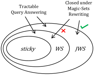
Figure 1: The existing and new settings

In relation to item (A) above, we consider both semantic and syntactic classes of Datalog^±.  By a semantic class of programs we refer to one whose programs also include their EDBs, and with that EDB the chase exhibits a certain behavior and has some special properties. A syntactic class characterizes its members, i.e. programs, in terms of a condition that is computable or decidable on the basis of the program’s rules alone, without involving an EDB (e.g. Sticky and WS Datalog^± are syntactic classes). A particularly prominent semantic condition (or class of programs that satisfy it) is that of stickiness of the chase (in short, the sch-property):

$${\it SCh} : \mathcal{P}\cup D$$ A program belongs to the SCh class if, due to the enforcement (3)

of a rule during the chase, a value replaces a join variable in a rule

body, then that value is propagated through all the possible subsequent

chase steps, i.e. the value “sticks”.

Example 1.2.

(ex. 1.1 cont.) Consider programs $\mathcal{P}$ and $\mathcal{P}^{\prime}$ below, both with EDB $D=\{R(a,b)\}$.

$$\begin{array}[]{rcl c rcl}&\mathcal{P}&&&&\mathcal{P}^{\prime}&\\ R(x,y)&~{}\rightarrow&~{}\exists z\;R(y,z),&&R(x,y)&~{}\rightarrow&~{}\exists z\;R(y,z),\\ R(x,y),R(y,z)&~{}\rightarrow&~{}S(x,y,z).&&R(x,y),R(y,z)&~{}\rightarrow&~{}S(x,y,z),\\ &&&&S(x,y,z)&~{}\rightarrow&~{}P(x,z).\end{array}$$

Figure 2: The sch-property.

$\mathcal{P}$ has the sch-property, as a portion of its chase in Figure 2(a) shows. $\mathcal{P}^{\prime}$ does not have the sch-property, as shown in Figure 2(b): value $b$ is not propagated to $P(a,\zeta_{1})$. $\blacksquare$

Stickiness of the chase defines a semantic class of programs in the sense that they involve an EDB. This class, SCh, contains every Sticky Datalog^± program [22] accompanied by any EDB, as long as the latter is schema-compatible with the program. So, in this case, a purely syntactic property of the program, independent from the EDB, guarantees stickiness.  For a program, stickiness of the chase, i.e. membership of SCh, guarantees tractability of QA, because CQs on such a program can be answered on an initial portion of the chase that has a fixed depth that is independent from the EDB (but depends only on the program and the query), and has a size that is polynomially bounded by the size of the EDB [22].

The class of WS Datalog^± programs we start from is defined in such a way it is guaranteed that values not appearing in any finite-rank position in a body join are propagated all the way up through the chase, for every EDB. Without going into the technical details about finite-rank positions for the moment, let’s just say that they are all finite positions of the program, where, for a program $\mathcal{P}\cup D$, a a position is finite if and only if finitely many different values may appear in it during the chase.  Accordingly, if we denote with ${\it FinPos}(\mathcal{P}\cup D)$ the set of finite positions of a program $\mathcal{P}\cup D$ consisting of a set of rules $\mathcal{P}$ and extensional database $D$, the set of finite-rank positions of $\mathcal{P}$ is contained in ${\it FinPos}(\mathcal{P}\cup D)$ (for every $D$). (There may be positions in ${\it FinPos}(\mathcal{P}\cup D)$ that are not finite-rank positions of $\mathcal{P}$ though.)

We can see that the definition of WS Datalog^±: (a) is based on a very particular way of choosing finite positions of the program; and (b) is crafted to guarantee that join values not appearing in those finite positions have the propagation property in relation to the chase. So, WS Datalog^± is in essence determined by a selection function (of finite positions), which is denoted by $\mathcal{S}^{\it rank}$, and turns out to be syntactic in the sense that in can be computed from the program $\mathcal{P}$, independently from $D$ (cf. Section 2.3.4).

This idea can be generalized in a very natural manner by replacing in (3), the condition “join variable” by the stronger one requiring “join variable not appearing in any of the finite positions selected by $\mathcal{S}$”, where $\mathcal{S}$ is an abstract selection function $\mathcal{S}$ that identifies a set of finite positions, say the “​$\mathcal{S}$-finite positions”, i.e. $\mathcal{S}(\mathcal{P}\cup D)\subseteq{\it FinPos}(\mathcal{P}\cup D)$, a possibly proper inclusion.

$$\mbox{{\it sch}}(\mathcal{S}) : \mbox{\em A program }\mathcal{P}\cup D\ \mbox{\em belongs to the }\mbox{{\it sch}}(\mathcal{S})\mbox{\em class if, due to the enforcement}$$ (4)

of a rule during the chase, a value replaces a join variable in the rule

$$\mbox{\em body that does not appear in any position in }\mathcal{S}(\mathcal{P}\cup D),\mbox{\em then that value}$$

is propagated through all the possible subsequent chase steps.

Since the condition on the join variables is stronger than that for sch, the new property defines a possibly larger semantic class of programs (the positions that have to be checked for value propagation may be a subset of those to check for SCh). For this class of programs sch$(\mathcal{S})$ that enjoy the $\mathcal{S}$-stickiness property of the chase, it holds  ${\it SCh}\subseteq\mbox{{\it sch}}(\mathcal{S})$.

We can define a whole range of program classes by considering different selection functions. There are two extreme cases. On one side, if $\mathcal{S}$ returns the empty set of finite positions, we reobtain Sch in (3). At the other extreme, if $\mathcal{S}$ selects all the finite positions, i.e. $\mathcal{S}(\mathcal{P}\cup D):={\it FinPos}(\mathcal{P}\cup D)$, then we obtain the class GSCh of programs with the generalized-stickiness property of the chase: A program $\mathcal{P}\cup D$ belongs to the GSCh class if, due to the enforcement of a rule during the chase, a value replaces a join variable in the rule body that does not appear in any position in ${\it FinPos}(\mathcal{P}\cup D)$, then that value is propagated through all the possible subsequent chase steps.

Clearly the GSCh class contains the SCh class, and all the other classes sch$(\mathcal{S})$. We should notice that, given a Datalog⁺ program $\mathcal{P}\cup D$, computing (deciding) ${\it FinPos}(\mathcal{P}\cup D)$ is unsolvable (undecidable) [26]. Accordingly, it is also undecidable if a Datalog⁺ program belongs to the GSCh class. The same may happen with some of the other sch$(\mathcal{S})$ classes.

As another particular case of (4), we obtain the semantic class sch($\mathcal{S}^{\it rank}$) related to WS Datalog^± by using the syntactic selection function $\mathcal{S}^{\it rank}$ that characterizes the finite-rank positions (cf. Section 2.3.4). Although WS Datalog^± is a syntactic class (membership does not depend on the EDBs), sch($\mathcal{S}^{\it rank}$) is still semantic, because -even with a syntactic $\mathcal{S}$- the stickiness property may depend on the EDB. However, every program in the syntactic WS Datalog^± class belongs to sch($\mathcal{S}^{\it rank}$), for every EDB.

In Section 3.4 we will introduce another syntactic selection function, $\mathcal{S}^{\exists}$, that will lead to the semantic class sch$(\mathcal{S}^{\exists})$. The associated syntactic class will be that of JWS Datalog^±. $\mathcal{S}^{\exists}$ that is inspired by the existential dependency graph of a program [31]. Since $\mathcal{S}^{\it rank}(\mathcal{P}\cup D)\subseteq\mathcal{S}^{\exists}(\mathcal{P}\cup D)\subseteq{\it FinPos}(\mathcal{P}\cup D)$, it holds sch($\mathcal{S}^{\it rank}$) $\subseteq$ sch($\mathcal{S}^{\exists}$). The programs in the associated syntactic class JWS Datalog^± will all belong to sch($\mathcal{S}^{\exists}$), for every EDB.  The containment relationships between the syntactic and semantic classes discussed so far are shown in Figure 3, with containment from left to right.  We define the semantic classes in Section 3, generalizing sticky Datalog^± on the basis of the classical chase.

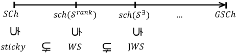
Figure 3: Some program classes in the range

We propose a general QA algorithm for the sch$(\mathcal{S})$ classes (cf. Section 4). It assumes that the positions identified by the selection $\mathcal{S}$ are computationally accessible, which may happen through an efficient, data-independent computation as in the case of syntactic classes above, or through an oracle that just returns them (say, in constant time) when $\mathcal{S}$ is not computable (and the finiteness of the positions it returns may depend on the data).

More precisely, the algorithm relies on the stickiness property of the chase for the program class at hand; and becomes of polynomial-time in data complexity, modulo access to sch$(\mathcal{S})$, on the assumption that $\mathcal{S}$ returns positions where polynomially many values appear during the chase. This is the case, in particular, for the semantic classes sch($\mathcal{S}^{\it rank}$) and sch$(\mathcal{S}^{\exists})$. Therefore, we obtain polynomial-time QA algorithms for their syntactic subclasses, WS and JWS Datalog^±, resp.

In general terms, the just described approach to QA works as follows: Given a query over a program in sch$(\mathcal{S})$, the $\mathcal{S}$-stickiness property of the program restricts the number of values that replace the join variables in non-$\mathcal{S}$-finite positions, because those values are propagated all the way to the query atom, which has a fixed arity. On the other hand, the join variables in $\mathcal{S}$-finite positions can only be replaced with finitely many values. As a result, the depth of the proof-schema, which depends on these join values, is also limited by the size of the query and the number of values in $\mathcal{S}$-finite positions. This guarantees the decidability of QA for programs in sch$(\mathcal{S})$. Furthermore, if the number of those join values is polynomial in the size of the EDB, the depth of proof-schema will be polynomial in EDB,  and QA becomes tractable.

The paper is structured as follows: Section 2 is a review of some basics of the database theory, the chase procedure, and Datalog^± program classes. Section 3 contains our semantic and syntactic generalizations of stickiness using selection functions. Section 4 and Section 5 contain the QA algorithm and MagicD⁺​. In this paper we use mainly intuitive and informal introductions of concepts and techniques, illustrated by examples. This work extends and is build upon our earlier work on QA for extensions of WS Datalog^± programs [38, 40].

2 Preliminaries and Background

In this section, we briefly review relational databases and the Datalog^± program classes.

2.1 Relational Databases

We consider relational schemas $\mathcal{R}$ with two disjoint domains: $\Gamma^{C}$, with possibly infinitely many constants, and $\Gamma^{N}$, of infinitely many labeled nulls. $\mathcal{R}$ also contains predicates of fixed finite arities. If $P$ is an $n$-ary predicate (i.e. with $n$ arguments) and $1\leq i\leq n$, $P[i]$ denotes its $i$-th position. $\mathcal{R}$ gives rise to a language $\mathfrak{L}(\mathcal{R})$ of first-order (FO) predicate logic with equality ($=$). Variables are usually denoted with $x,y,z,...$, and finite sequences thereof by $\bar{x},...$. Constants are usually denoted with $a,b,c,...$; and nulls are denoted with $\zeta,\zeta_{1},...$. An atom is of the form $P(t_{1},\ldots,t_{n})$, with $P$ an $n$-ary predicate and $t_{1},\ldots,t_{n}$ terms, i.e. constants, nulls, or variables. The atom is ground (aka. a tuple) if it contains no variables. An instance $I$ for schema $\mathcal{R}$ is a possibly infinite set of ground atoms. The active domain of an instance $I$, denoted ${\it Adom}(I)$, is the set of constants and nulls that appear in atoms of $I$. Instances can be used as interpretation structures for language $\mathfrak{L}(\mathcal{R})$. A database instance is a finite instance that contains no nulls.

A homomorphism from instance $I$ to instance $I^{\prime}$ for the same schema is a structure-preserving mapping, ${\it Adom}(I)\!\rightarrow\!{\it Adom}(I^{\prime})$, such that: (a) $t\in\Gamma^{C}$ implies $h(t)=t$, and (b) for every ground atom $P(\bar{t})\in I$, it holds $P(h(\bar{t}))\in I^{\prime}$. ($h(\bar{t})$ is defined componentwise.)

A conjunctive query (CQ) is a FO formula, $\mathcal{Q}(\bar{x})$, of the form:

$$\exists\bar{y}\;(P_{1}(\bar{x}_{1})\wedge\dots\wedge P_{n}(\bar{x}_{n})),$$ (5)

with (distinct) free variables $\bar{x}:=(\bigcup\bar{x}_{i})\smallsetminus\bar{y}$. If $\mathcal{Q}$ has $m$ (free) variables, for an instance $I$, $\bar{t}\in(\Gamma^{C}\cup\Gamma^{N})^{m}$  is an answer to $\mathcal{Q}$ if $I\models\mathcal{Q}[\bar{t}]$, meaning that $Q[\bar{t}]$ becomes true in $I$ when the variables in $\bar{x}$ are componentwise replaced by the values in $\bar{t}$. $\mathcal{Q}(I)$ denotes the set of answers to $\mathcal{Q}$ in $I$. $\mathcal{Q}$ is a boolean conjunctive query (BCQ) when $\bar{x}$ is empty; and if it is true in $I$, $\mathcal{Q}(I):=\{{\it true}\}$. Otherwise, $\mathcal{Q}(I)=\emptyset$, and we say it is false.

A tuple-generating dependency (tgd), also called a rule, is an implicitly universally quantified sentence of $\mathfrak{L}(\mathcal{R})$ of the form:

$$\sigma\!:\ \ P_{1}(\bar{x}_{1}),\ldots,P_{n}(\bar{x}_{n})\ \rightarrow\ \exists\bar{y}\ P(\bar{x},\bar{y}),$$ (6)

with $\bar{x}\subseteq\bigcup_{i}\bar{x}_{i}$, and the dots in the antecedent standing for conjunctions. The variables in $\bar{y}$ (that could be empty) are the existential variables. We assume $\bar{y}\cap\cup\bar{x}_{i}=\emptyset$. With ${\it head}(\sigma)$ and ${\it body}(\sigma)$ we denote the atom in the consequent and the set of atoms in the antecedent of $\sigma$, respectively. A tgd may contain constants from $\Gamma^{C}$ in predicate positions.

A constraint is an equality-generating dependency (egd) or a negative constraint (nc), which are also sentences of $\mathfrak{L}(\mathcal{R})$, respectively, of the forms:

$$P_{1}(\bar{x}_{1}),\ldots,P_{n}(\bar{x}_{n})\ \rightarrow\ x=x^{\prime},$$ (7)

$$P_{1}(\bar{x}_{1}),\ldots,P_{n}(\bar{x}_{n})\ \rightarrow\ \bot,$$ (8)

where $x,x^{\prime}\in\bigcup_{i}\bar{x}_{i}$, and $\bot$ is a symbol that denotes the Boolean constant (propositional variable) that is always false. Satisfaction of constraints by an instance is as in FO logic. Tgds, egds, and ncs are particular kinds of relational integrity constraints (ICs) [1]. In particular, egds include key constraints and functional dependencies (FDs). ICs also include inclusion dependencies (IDs) that are subsumed by tgds.

Relational databases work under the closed world assumption (CWA) [1]: ground atoms not belonging to a database instance are assumed to be false. As a result of this form of data-completeness assumption, an IC is always true or false when checked for satisfaction on a database instance, never undetermined. As we will see below, if instances are allowed to be incomplete or open, i.e. with undetermined or missing ground atoms, ICs can be used, by enforcing them, to generate new tuples.

Datalog  is a declarative query language for relational databases that is based on the logic programming paradigm, and allows to define recursive views [1, 25]. A Datalog  program $\mathcal{P}$ for schema $\mathcal{R}$ is a finite set of non-existential rules, i.e. as in (6) above but without $\exists$-variables. Some of the predicates in $\mathcal{P}$ are extensional, i.e. they do not appear in rule heads, and the extensions for them (i.e. their sets of tuples) are given by a complete database instance $D$ (for the extensional subschema of $\mathcal{R}$), which is called the extensional database  (EDB). The other, intentional, predicates are defined by rules that have them in their heads. For Datalog programs, we may assume, without loss of generality, that intentional predicates appear only in rules, but not in the EDB.

The minimal-model semantics of a Datalog  program with respect to (wrt.) an extensional database instance $D$ is given by a fixed-point semantics: the extensions of the intentional predicates are obtained by, starting from $D$, iteratively enforcing the rules and creating tuples for the intentional predicates, i.e. whenever a ground (or instantiated) rule body becomes true in the extension obtained so far, but not the head, the corresponding ground head atom is added to the extension under computation. If the set of initial ground atoms is finite, the process reaches a fixed-point after a number of steps that is polynomially bounded in the size of $D$.

A CQ as in (5) can be expressed as a Datalog  rule of the form:

$$P_{1}(\bar{x}_{1}),...,P_{n}(\bar{x}_{n})\rightarrow{\it ans}_{\mathcal{Q}}(\bar{x}),$$ (9)

where ${\it ans}_{\mathcal{Q}}(\cdot)$ is an auxiliary, answer-collecting predicate. The answers to query $\mathcal{Q}$ form the extension of predicate ${\it ans}_{\mathcal{Q}}(\cdot)$ in the minimal model. When $\mathcal{Q}$ is a BCQ, ${\it ans}_{\mathcal{Q}}$ is a propositional atom; and $\mathcal{Q}$ is true in the undelying instance exactly when the atom ${\it ans}_{\mathcal{Q}}$ belongs to the minimal model of the program.

Example 2.1.

A Datalog  program $\mathcal{P}$ containing the rules

$$P(x,y)~{}\rightarrow~{}R(x,y),$$

$$P(x,y),R(y,z)~{}\rightarrow~{}R(x,z)$$

recursively defines, on top of the extensional relation $P$, the intentional predicate $R$ as the transitive closure of $P$. For $D=\{P(a,b),P(b,d)\}$ as extensional database, the extension of $R$ can be computed by iteratively adding tuples enforcing the program rules, which results in $\{R(a,b),R(b,d),R(a,d)\}$.

The CQ $\mathcal{Q}(x)\!:\ R(x,b)\wedge R(x,d)$ can be expressed by the rule  $R(x,b),R(x,d)$ $\rightarrow\ {\it ans}_{\mathcal{Q}}(x)$. The set of answer is the computed extension for ${\it ans}_{\mathcal{Q}}(x)$, namely $\{a\}$. $\blacksquare$

2.2 Datalog^±

Datalog^± is an extension of Datalog. The “$+$” stands for the extension, and the “$-$”, for some syntactic restrictions on the program that guarantee some good computational properties. We will refer to some of those restrictions in Section 2.3. Accordingly, until then we will consider Datalog⁺ programs.

A Datalog⁺ program may contain, in addition to (non-existential) Datalog rules, existential rules of the form (6), constraints of the forms (7) and (8), and a finite extensional database $D$ that may be incomplete and contains ground atoms for the extensional predicates, i.e. those that do not appear in rule heads, and possibly also for the intensional predicates, i.e. those appearing in rule heads.  We will usually denote with $\mathcal{P}$ the set of rules and constraints, and with $D$ the extensional database (EDB). Accordingly a program is of the form $\mathcal{P}\cup D$. When no possible confusion arises, we simply refer to $\mathcal{P}$ as the “program”.  A program has an associated schema formed by the predicates in it.  The set of positions (for the predicates) in a program $\mathcal{P}$ is denoted with ${\it Pos}(\mathcal{P})$.  We may safely assume all the predicates in an EDB for program $\mathcal{P}$ also appear in $\mathcal{P}$.

The semantics of a Datalog⁺ program $\mathcal{P}\cup D$ is model-theoretic, and given by the class ${\it Mod}(\mathcal{P},D)$ of all instances $D^{\prime}$ for the program’s schema that extend $D$ and make $\mathcal{P}$ true. In particular, given a an $n$-ary CQ $\mathcal{Q}(\bar{x})$, $\bar{t}\in(\Gamma^{C}\cup\Gamma^{N})^{n}$ is an answer wrt. $\mathcal{P}$ and $D$ iff $D^{\prime}\models\mathcal{Q}[\bar{t}]$ for every $D^{\prime}\in{\it Mod}(\mathcal{P},D)$. This is certain answer semantics that requests truth in all models. Without any restrictions on the program, and even for programs without constraints, conjunctive query answering (CQA) may be undecidable [10].

CQA appeals to all possible models of the program. However, the chase procedure [34] can be used to generate a single instance that represents the class ${\it Mod}(\mathcal{P},D)$ for this purpose. We show it by means of an example containing only tgds.

Example 2.2.

Consider a program $\mathcal{P}$ with the set of rules  $\sigma\!:R(x,y)\ \rightarrow\ \exists z\ R(y,z)$,  and  $\sigma^{\prime}\!:R(x,y),R(y,z)\ \rightarrow\ S(x,y,z)$, and an extensional instance $D=\{R(a,b)\}$, providing an incomplete extension for the program’s schema. With the $I_{0}:=D$, the pair $(\sigma,\theta_{1})$, with (value) assignment (for variables) $\theta_{1}\!:\ x\mapsto a,y\mapsto b$, is applicable: $\theta_{1}({\it body}(\sigma))=\{R(a,b)\}\subseteq I_{0}$. The chase enforces $\sigma$ by inserting a new tuple $R(b,\zeta_{1})$ into $I_{0}$, with $\zeta_{1}$ a fresh null, i.e. not in $D_{0}$, resulting in instance $I_{1}=\{R(a,b),R(b,\zeta_{1})\}$. This chase step is denoted as  $I_{0}\rightarrow_{(\sigma,\theta_{1})}I_{1}$.

Now, $(\sigma^{\prime},\theta_{2})$, with $\theta_{2}\!:\ x\mapsto a,y\mapsto b,z\mapsto\zeta_{1}$, is applicable in $I_{1}$, because $\theta_{2}({\it body}(\sigma^{\prime}))$ $=$ $\{R(a,b),R(b,\zeta_{1})\}\subseteq I_{1}$. The chase adds $S(a,b,\zeta_{1})$ into $I_{1}$, resulting in instance $I_{2}$. The chase continues, without stopping, creating an infinite instance, usually called the chase (instance):

$${\it chase}(\mathcal{P},D)=\{R(a,b),R(b,\zeta_{1}),S(a,b,\zeta_{1}),R(\zeta_{1},\zeta_{2}),R(\zeta_{2},\zeta_{3}),S(b,\zeta_{1},\zeta_{2}),\ldots\}.$$

A query over $\mathcal{P}\cup D$ can be answered on a finite, initial portion of the infinite chase instance. For example, only after adding $R(b,\zeta_{1})$, we can return true as the answer to the BCQ $\mathcal{Q}:\exists x\;R(b,x)$. For certain syntactic classes of programs, such as the “sticky” program in this example (c.f. Section 2.3), it is also possible to return a negative answer to BCQ. For example, we can return false as the answer to $\mathcal{Q}^{\prime}:\exists x,y\;S(x,y,a)$ after a finite number of chase steps, confirming that constant $a$ will never occur in position $S[3]$. For a given program (with the right properties), the size of the initial, finite portion of the chase for QA depends on the query. For example, to answer $\mathcal{Q}^{\prime\prime}:\exists x,y,z,w,u\;(S(x,y,z)\wedge S(y,z,w)\wedge S(z,w,u)$, actually positively, we need to generate more atoms than those needed to answer $\mathcal{Q}$, to map them to the three atoms in $\mathcal{Q}^{\prime\prime}$. $\blacksquare$

Some natural questions arise from Example 2.2, among them: Assuming the program has good properties in relation to the chase (say it belongs to one of the classes we investigate in this work), (a) How far do we have to finitely develop the chase to correctly answer a given CQ?  (b) How does it depend on the query?  (c) Having that finite portion of the chase, possibly materialized, what other CQs can be answered on that portion?  We address these question in Section 4.

In a nutshell, we use a modified version of the chase that includes two special ingredients, namely homomorphism checking along the chase, and “freezing” of some nulls, i.e. treating them as constants. The latter technique was introduced in [33] for a different program class. The application of these two elements depend on the query, and produces a finite portion of the (classical) chase that is large enough to correctly answer the query.

Depending on the programs and instances, the chase may be finite or infinite; and different orders of chase steps may result in different sequences and instances. However, it is possible to define a canonical chase procedure that determines a canonical sequence of chase steps, and consequently, a canonical chase instance [23].

Given a program $\mathcal{P}$ and EDB $D$, the chase (instance) is a universal model [27]: For every $I\in{\it Mod}(\mathcal{P},D)$, there is a homomorphism from the chase into $I$. For this reason, the (certain) answers to a CQ $\mathcal{Q}$ under $\mathcal{P}$ and $D$ can be computed by evaluating $\mathcal{Q}$ over the chase instance (discarding the answers containing nulls) [27].

If the program $\mathcal{P}\cup D$ has ncs, they are expected to be satisfied by the chase. That is, the BCQ associated to the nc (8), i.e. $\mathcal{Q}_{\eta}\!:\ \exists\bar{x}_{1}\cdots\bar{x}_{n}(P_{1}(\bar{x}_{1})\wedge\cdots\wedge P_{n}(\bar{x}_{n})$, obtained from the the body of (8), must be false. If this is not the case, we say $\mathcal{P}$ is inconsistent. If $\mathcal{P}$ has egds, they are also expected to be satisfied by the chase. However, one can modify the chase in order to enforce the egds, which may be possible or not. In the latter case, we say the chase fails. (It is possible to define a canonical chase that involves egds [23].)

Example 2.3.

Consider a program $\mathcal{P}$ with $D=\{R(a,b)\}$ with two rules and an egd:

$$R(x,y)~{} \rightarrow~{}\exists z\;\exists w\;S(y,z,w),$$ (10)

$$S(x,y,y)~{} \rightarrow~{}P(x,y),$$ (11)

$$S(x,y,z)~{} \rightarrow~{}y=z.$$ (12)

The chase of $\mathcal{P}$ first applies (10) and results in $I_{1}=\{R(a,b),S(b,\zeta_{1},\zeta_{2})\}$. There are no more tgd/assignment applicable pairs. But, if we enforce the egd (12), equating $\zeta_{1}$ and $\zeta_{2}$, we obtain $I_{2}=\{R(a,b),S(b,\zeta_{1},\zeta_{1})\}$. Now, (11) and $\theta^{\prime}:x\mapsto b,y\mapsto\zeta_{1}$ are applicable, so we add $P(b,\zeta_{1})$ to $I_{2}$, generating $I_{3}=\{R(a,b),S(b,\zeta_{1},\zeta_{1}),P(b,\zeta_{1})\}$. The chase terminates (no applicable tgds or egds), obtaining ${\it chase}(\mathcal{P},D)=I_{3}$.  Notice that the program consisting only of (10) and (11) produces $I_{1}$ as the chase, which makes the BCQ $\exists x\exists yP(x,y)$ evaluate to false. With the program also including the egd (12) the answer is now true.

Now consider program $\mathcal{P}^{\prime}$ that is $\mathcal{P}$ with the extra rule  $R(x,y)~{}\rightarrow~{}\exists z\;S(z,x,y)$, which enforced on $I_{3}$ results in $I_{4}=\{R(a,b),S(b,\zeta_{1},\zeta_{1}),P(b,\zeta_{1}),S(\zeta_{3},a,b)\}$. Now (12) is applied, which creates a chase failure as it tries to equate constants $a$ and $b$. In this case the set of tgds and the egd are mutually inconsistent. $\blacksquare$

Characterizations of computationally well-behaved classes of Datalog^± programs usually do not consider any kind of egds and ncs in the program, but only the tgds. However, considering ncs is not complicated for these characterizations since they may have a trivial effect of QA or no effect at all. More precisely, if a program $\mathcal{P}$ consists of a set of tgds $\mathcal{P}^{R}$ and a set of ncs $\mathcal{P}^{C}$, then CQA amounts to deciding if $\mathcal{P}^{R}\cup\mathcal{P}^{C}\cup D\models\mathcal{Q}$, for which the following result holds.

Proposition 1.

[22, theo. 6.1] $\mathcal{P}^{R}\cup\mathcal{P}^{C}\cup D\models\mathcal{Q}$  iff  (a) $\mathcal{P}^{R}\cup D\models\mathcal{Q}$,  or  (b) for some $\eta\in\mathcal{P}^{C}$, $\mathcal{P}^{R}\cup D\models\mathcal{Q}_{\eta}$, where $\mathcal{Q}_{\eta}$ is the BCQ obtained as the existential closure of the body of $\eta$. $\blacksquare$

Proof:  ​​  Assume (b) does not hold, then ${\it Mod}(\mathcal{P}^{R}\cup\mathcal{P}^{C}\!,D)\neq\emptyset$. We have to show that $\mathcal{P}^{R}\cup\mathcal{P}^{C}\cup D\models\mathcal{Q}$ iff $\mathcal{P}^{R}\cup D\models\mathcal{Q}$. From right to left is obvious. Now, from left to right, assume $\mathcal{P}^{R}\cup\mathcal{P}^{C}\cup D\models\mathcal{Q}$, and let $D^{\prime}\in{\it Mod}(\mathcal{P}^{R},D)$. We have to show that $I\models\mathcal{Q}$. Let $I^{{\it ch}}$ be ${\it chase}(\mathcal{P}^{R},D)$, for which $I^{{\it ch}}\models\mathcal{P}^{C}$ holds (otherwise, due to the universality of the chase and preservation of CQA under homomorphisms, $\mathcal{P}^{R}\cup\mathcal{P}^{C}\cup D$ would be inconsistent). Then, $I^{{\it ch}}\in{\it Mod}(\mathcal{P}^{R}\cup\mathcal{P}^{C},D)$, and then, by hypothesis, $I^{{\it ch}}\models\mathcal{Q}$. Since $I^{{\it ch}}$ can be homomorphically embedded into $I$, we obtain  $I\models\mathcal{Q}$. $\blacksquare$

Case (b) above holds exactly when $\mathcal{P}\cup D$ is inconsistent, and $\mathcal{Q}$ becomes trivially true. This shows that CQA evaluation under ncs can be reduced to the same problem without ncs, and the data complexity of CQA does not change. Furthermore, ncs may have an effect on CQA only if they are mutually inconsistent with the rest of the program, in which case every BCQ becomes trivially true. The presence of egds may have a more dramatic effect of QA, which can become undecidable, and the presence of egds may also change query answers, as in Example 2.3 (cf. [13, sec. 2] for a more detailed discussion).  As a consequence, we assume in the rest of this work that programs do not have egds  or ncs.

2.3 Programs Classes

CQ answering over Datalog⁺ programs with arbitrary sets of tgds is undecidable [10]. Actually, it is undecidable whether the chase terminates, even for a fixed instance [10, 26]. Several sufficient conditions, syntactic [26, 27, 31, 37] or data-dependent [35], that guarantee chase termination have been identified. Weak-acyclicity [27] and joint-acyclicity [31] are syntactic conditions that use a static analysis of a dependency graph of predicate positions in the program.

A non-terminating chase does not imply that CQ answering is undecidable. Several program classes are identified for which the chase may be infinite, but QA is still decidable. That is the case for linear, guarded, sticky, weakly-sticky Datalog^± [16, 17, 19, 22], shy Datalog^∃ [33], and finite expansion sets (fes), finite unification sets (fus), bounded-treewidth sets (bts) [6, 7, 8]. Each program class defines conditions on the program rules that lead to good computational properties for QA. In the following, we focus on Sticky and WS Datalog^± programs.

2.3.1 Weakly-acyclic programs

The dependency graph (DG) of a program $\mathcal{P}$ with schema $\mathcal{R}$ (cf. Figure 4) is a directed graph whose vertices are the positions (of predicates) in $\mathcal{P}$. The edges are defined as follows: for every $\sigma\in\mathcal{P}$, and every universally quantified variable ($\forall$-variable) $x$ in ${\it head}(\sigma)$ in position $p$ in ${\it body}(\sigma)$ (among possibly other positions where $x$ appears in ${\it body}(\sigma)$):  (a) for each occurrence of $x$ in position $p^{\prime}$ in ${\it head}(\sigma)$, create an edge from $p$ to $p^{\prime}$, (b) for each $\exists$-variable $z$ in position $p^{\prime\prime}$ in ${\it head}(\sigma)$, create a special (dashed) edge from $p$ to $p^{\prime\prime}$.

The rank of a position $p$ in the graph, denoted by ${\it rank}(p)$, is the maximum number of special edges over all (finite or infinite) paths ending at $p$. $\Pi_{F}(\mathcal{P})$ and $\Pi_{\infty}(\mathcal{P})$ denote the sets of finite-rank and infinite-rank positions in $\mathcal{P}$, resp. It is possible to prove that finite-rank positions are finite positions, i.e. they belong to ${\it FinPos}(\mathcal{P}\cup D)$ for every EDB $D$ [27].  A program is weakly-acyclic (WA) if all of the positions belong to $\Pi_{F}(\mathcal{P})$ [27].

Example 2.4.

Let $\mathcal{P}$ be a program with rules:

$$R(x,y),R(y,z) ~{}\rightarrow~{}R(x,z),$$

$$R(x,y) ~{}\rightarrow~{}\exists z\;P(y,z).$$

The DG  of $\mathcal{P}$ is shown in Figure 4. Positions $R[1]$, $R[2]$ and $P[1]$ have rank $0$; and $P[2]$, rank $1$.  $\mathcal{P}$ is WA since all positions have finite-rank. There is a cycle in the DG of $\mathcal{P}$, but it does not involve any special edge.

Now, let $\mathcal{P}^{\prime}$ be WS program with rules:

$$R(x,y) ~{}\rightarrow~{}P(y,x),$$

$$P(x,y) ~{}\rightarrow~{}\exists z\;R(y,z).$$

The DG of $\mathcal{P}^{\prime}$ is shown in Figure 5. Positions $R[1]$ and $P[2]$ have rank $0$. The program is not WA since $R[2]$ and $P[1]$ have infinite rank. $\mathcal{P}^{\prime}$ is not WS, because its DG graph has a cycle with a special edge. $\blacksquare$

Figure 4: Dependency graph of $\mathcal{P}$

oo

Figure 5: Dependency graph of $\mathcal{P}^{\prime}$

The problem of BCQ answering over a WA program is ptime-complete in data complexity [27]. This is because the chase for these programs stops in polynomial time in the size of the data [27]. The same problem is 2exptime-complete in combined complexity, i.e. in the size of both program rules and the data [30].

2.3.2 Jointly-acyclic programs

The definition of the class of jointly-acyclic (JA) programs appeals to the existential dependency graph (EDG) of a program $\mathcal{P}$ [31], denoted EDG$(\mathcal{P})$, that we briefly review here.

Assume that program $\mathcal{P}$ has its rules standardized apart, i.e. no variable appears in more than one rule. For a variable $x$ in rule $\sigma$, let $B_{x}$ and $H_{x}$ be the sets of positions where $x$ occurs in the body, resp. in the head, of $\sigma$. For an $\exists$-variable $z$, the set of target positions of $z$, denoted by $T_{z}$, is the smallest set of positions such that: (a) $H_{z}\subseteq T_{z}$, and (b) $H_{x}\subseteq T_{z}$ for every $\forall$-variable $x$ with $B_{x}\subseteq T_{z}$. Roughly speaking, $T_{z}$ is the set of positions where the invented (fresh) null values for the $\exists$-variable $z$ may appear during the chase.

EDG$(\mathcal{P})$ is a directed graph with the $\exists$-variables of $\mathcal{P}$ as its nodes. There is an edge from $z\in\sigma$ to $z^{\prime}\in\sigma^{\prime}$ if there is a body variable $x$ in $\sigma^{\prime}$ such that $B_{x}\subseteq T_{z}$. Intuitively, the edge shows that the values invented by $z$ may appear in the body of $\sigma^{\prime}$, and cause (null) value invention for $z^{\prime}$. Therefore, a cycle represents the possibility of inventing infinitely many null values for the $\exists$-variables in the cycle. A program is jointly-acyclic (JA) if its EDG  is acyclic.

Example 2.5.

Consider a program $\mathcal{P}$ with the following rules:

$$P(x_{1},y_{1})\!~{} \rightarrow~{}\!\exists z_{1}\ R(y_{1},z_{1}),$$ (13)

$$R(x_{2},y_{2}),U(x_{2}),U(y_{2})\!~{} \rightarrow~{}\!\exists z_{2}\ P(y_{2},z_{2}),$$ (14)

$$P(x_{3},y_{3})\!~{} \rightarrow~{}\!\exists z_{3}\ S(x_{3},y_{3},z_{3}).$$ (15)

Figure 6: EDG$(\mathcal{P})$

$B_{y_{1}}=\{P[2]\}$ and $H_{y_{1}}=\{R[1]\}$ are the sets of positions where the variable $y_{1}$ appears in the body and, resp. the head of rule (13). Similarly, $B_{x_{2}}=\{R[1],U[1]\}$, $B_{y_{2}}=\{R[2],U[1]\}$, and $B_{y_{3}}=\{P[2]\}$. $T_{z_{1}}=\{R[2]\}$ and $T_{z_{2}}=\{P[2],R[1],S[2]\}$ are the sets of target positions of $z_{1}$ and resp. $z_{2}$.

In EDG$(\mathcal{P})$ in Figure 6 there is an edge from $z_{2}$ to $z_{1}$ since for the body variable $y_{1}$ in rule (13), where $z_{1}$ appears, $B_{y_{1}}\subseteq T_{z_{2}}$ holds, which means $y_{1}$ occurs only in the target positions of $z_{2}$. Similarly, there is an edge from $z_{2}$ to $z_{3}$ since for the body variable $y_{3}$ in rule (15), where $z_{3}$ appears, $B_{y_{3}}\subseteq T_{z_{2}}$ holds, which means $y_{3}$ occurs only in the target positions of $z_{2}$. There is no edge from $z_{1}$ to $z_{2}$ since, in rule (14), $B_{x_{2}}\not\subseteq T_{z_{1}}$ and $B_{y_{2}}\not\subseteq T_{z_{1}}$. For a similar reason, there is no self-loop for $z_{2}$. The graph is acyclic, and then, $\mathcal{P}$ is JA. $\blacksquare$

JA programs have polynomial size (finite) chase wrt. the size of the extensional data, and properly extend WA programs. BCQ answering over JA programs is ptime-complete in data complexity, and 2exptime-complete is combined complexity [31].

2.3.3 Sticky programs

They are characterized through a body variable marking procedure whose input is the set of rules of a program $\mathcal{P}$ (the extensional data do not participate in it). The procedure has two steps:

• Preliminary step: For each $\sigma\in\mathcal{P}$ and variable $x$ in ${\it body}(\sigma)$, if there is an atom $A$ in ${\it head}(\sigma)$ where $x$ does not appear, mark each occurrence of $x$ in ${\it body}(\sigma)$.

• Propagation step: For each $\sigma\in\mathcal{P}$, if a marked variable in ${\it body}(\sigma)$ appears in position $p$, then for every $\sigma^{\prime}\in\mathcal{P}$ (including $\sigma$), mark the variables in ${\it body}(\sigma^{\prime})$ that appear in ${\it head}(\sigma^{\prime})$ in position $p$.

We say that $\mathcal{P}$ is sticky (or belongs to the program class Sticky) when, after applying the marking procedure, there is no rule with a marked variable appearing more than once in its body (i.e. not a join variable). Notice that a variable never appears both marked and unmarked in a same body.

Example 2.6.

(ex. 1.2 cont.) For program $\mathcal{P}$ on the left-hand side below, the first rule below already shows marked variable $x$ (with a hat) after the preliminary step. The set of rules on the right-hand side is the final result of the marking procedure applied to $\mathcal{P}$:

$$\begin{array}[]{rcl c rcl}R(\hat{x},y)&~{}\rightarrow&~{}\exists z\;R(y,z),&&R(\hat{x},\hat{y})&~{}\rightarrow&~{}\exists z\;R(y,z),\\ R(x,y),R(y,z)&~{}\rightarrow&~{}S(x,y,z),&&R(x,y),R(y,z)&~{}\rightarrow&~{}S(x,y,z).\end{array}$$

Variable $y$ in the first rule-body ends up marked after the propagation step: it appears in the rule head, in position $R[1]$, where marked variable $x$ appear in the same rule. Accordingly, $\mathcal{P}$ is sticky: there is no marked variable that appears more than once in a rule body.

For program $\mathcal{P}^{\prime}$, the result of the marking procedure is as follows:

$$\begin{array}[]{rl}R(\hat{x},\hat{y})&~{}\rightarrow~{}\exists z\;R(y,z).\\ R(x,\hat{y}),R(\hat{y},z)&~{}\rightarrow~{}S(x,y,z).\\ S(x,\hat{y},z)&~{}\rightarrow~{}P(x,z).\end{array}$$

$\mathcal{P}^{\prime}$ is not sticky: $y$ in the second rule body is marked and occurs twice in it (in $R[2]$ and $R[1]$). $\blacksquare$

The syntactic stickiness condition guarantees that QA can be done in ptime in data complexity; and is exptime-complete in combined complexity [22]. The chase of a Sticky program may not terminate, as shown in Example 2.6. However, a CQ can be answered by rewriting it into a FO query, actually a union of CQs, doing backward-chaining through the rules, and answering the FO query directly on the EDB. The rewriting depends only on the rules and the query; and the size of the rewriting is independent from the EDB [22, 28].

2.3.4 Weakly-sticky programs

They form a syntactic class that extends those of WA and Sticky programs. Its characterization does not depend on the extensional data, and uses the notions of finite-rank and marked variable introduced in Sections 2.3.1 and 2.3.3, resp.: A set of rules $\mathcal{P}$ is weakly-sticky (WS) if, for every rule in it and every repeated variable in its body, the variable is either non-marked or appears in a position in $\Pi_{F}(\mathcal{P})$.

Example 2.7.

Consider $\mathcal{P}$ with the set of rules:

$$R(x,y)~{}\rightarrow ~{}\exists z\;R(y,z),$$

$$R(x,y),U(y),R(y,z)~{}\rightarrow ~{}R(x,z),$$

for which $\Pi_{F}(\mathcal{P})=\{U[1]\}$ and $\Pi_{\infty}(\mathcal{P})=\{R[1],R[2]\}$. After applying the marking procedure, every body variable in $\mathcal{P}$ becomes marked. $\mathcal{P}$ is WS since the only repeated marked variable is $y$, in the second rule, and it appears in $U[1]\in\Pi_{F}(\mathcal{P})$.

Now, let $\mathcal{P}^{\prime}$ be the program with the first rule of $\mathcal{P}$ and the second rule as follows:

$$R(x,y),R(y,z)~{}\rightarrow ~{}R(x,z).$$

Now, $\Pi_{F}(\mathcal{P}^{\prime})=\emptyset$ and $\Pi_{\infty}(\mathcal{P}^{\prime})=\{R[1],R[2]\}$. After applying the marking procedure, every body variable in $\mathcal{P}^{\prime}$ is marked. $\mathcal{P}^{\prime}$ is not WS since $y$ in the second rule is repeated, marked and appears in $R[1]$ and $R[2]$, both in $\Pi_{\infty}(\mathcal{P})$. $\blacksquare$

The WS condition guarantees tractability of CQ answering w.r.t. the size of the EDB [20]. Intuitively, WS generalizes the syntactic condition of sticky rules by preventing a repeated, marked variable from appearing only in infinite-rank positions, where it has no bound on the values it can take. However, appearing at least once in a finite position propagates boundedness to its other occurrences. For WS programs, QA can be done by rewriting a CQ into a union of CQs, and answering the resulting query over the EDB [20]. However, unlike Sticky programs, for WS programs the rewritten query and its size may depend on the EDB, but the latter is polynomially bounded by the size of the EDB.

3 Chase-Based Generalizations of Sticky Datalog^±

In Section 1 we stated our goal of identifying a class of Datalog^± programs that extends WS, has a tractable QA problem, and is also closed under magic-set optimization. These desiderata lead us to analyze more closely the syntactic conditions for Sticky and WS programs on one side, and, on the other side, value propagation under the chase for those classes.  In this section, generalizing from this analysis, we will characterize and use selection functions $\mathcal{S}$ that identify sets of finite positions of programs $\mathcal{P}\cup D$.

3.1 Selection Functions

Definition 1.

(a) A selection function $\mathcal{S}$ associates every program $\mathcal{P}\cup D$ with a subset $\mathcal{S}(\mathcal{P}\cup D)$ of ${\it FinPos}(\mathcal{P}\cup D)$, which is the set of positions that take finitely many values in ${\it chase}(\mathcal{P},D)$. (b) The selection functions $\mathcal{S}^{\bot}$,  $\mathcal{S}^{\top}$ and $\mathcal{S}^{\it rank}$ are defined by:  $\mathcal{S}^{\bot}(\mathcal{P}\cup D):=\emptyset$,  $\mathcal{S}^{\top}(\mathcal{P}\cup D):={\it FinPos}(\mathcal{P}\cup D)$, and $\mathcal{S}^{\it rank}(\mathcal{P}\cup D):=\Pi_{F}(\mathcal{P})$, the set of finite-rank positions of $\mathcal{P}$, resp. $\blacksquare$

Notice that $\mathcal{S}^{\top}$ is in general non-computable [26], but $\mathcal{S}^{\bot}$ is clearly computable. $\mathcal{S}^{\it rank}$ is a selection function because finitely many values appear in these positions during the chase of the program [27, Theorem 3.9]. It is also computable since the finite-rank positions can be computed from the dependency graph of the program.

Definition 2.

A selection function $\mathcal{S}$ is syntactic iff:  (a) there is a computable function $\mathcal{S}^{\prime}$ that associates each program $\mathcal{P}$ with a subset $\mathcal{S}^{\prime}(\mathcal{P})$ of  ${\it Pos}(\mathcal{P})$, such that $\mathcal{S}(\mathcal{P}\cup D)=\mathcal{S}^{\prime}(\mathcal{P})$, for every $D$;  and (b) $\mathcal{S}^{\prime}(\mathcal{P})\subseteq{\it FinPos}(\mathcal{P}\cup D)$, for every $D$. $\blacksquare$

Intuitively, the result of a syntactic selection function depends on the program, but not on the EDB. It soundly returns (some) positions that are finite for a program with any accompanying EDB. Both $\mathcal{S}^{\bot}$ and $\mathcal{S}^{\it rank}$ are syntactic selection functions, because they only depend on the program, not on the EDB. Particularly, $\mathcal{S}^{\it rank}$ only depends on the DG of the program, which is independent of the EDB. We will introduce a computable and syntactic selection function, $\mathcal{S}^{\exists}$, in Section 3.4.

3.2 Semantic Program Classes Defined by Selection Functions

In order to formally define stickiness properties of the chase, we first recall the chase relation, $<_{\mathcal{P},D}$, over the atoms in ${\it chase}(\mathcal{P},D)$ [22, def. 2.1.]. Intuitively, $A<_{\mathcal{P},D}B$ means that $B$ is obtained from $A$ (and possibly other atoms) in a chase step with $\mathcal{P}\cup D$ .

Definition 3 (Chase relation).

For a Datalog⁺ program $\mathcal{P}\cup D$, and atoms $A,B\in{\it chase}(\mathcal{P},D)$, $A$ is in chase relation to $B$, denoted $A<_{\mathcal{P},D}B$, if and only if there is a chase step $I_{i}\rightarrow_{(\sigma_{i},\theta_{i})}I_{i+1}$ with $\mathcal{P}\cup D$, such that $A\in\theta_{i}({\it body}(\sigma))$ and $B\in I_{i+1}\setminus I_{i}$. The derivation relation for $\mathcal{P}\cup D$, denoted by $\ll_{\mathcal{P},D}$, is the transitive closure of $<_{\mathcal{P},D}$. $\blacksquare$

Example 3.1.

(ex. 1.2 cont.) According to the chase with $\mathcal{P}\cup D$ in Figure 2, $R(a,b)<_{\mathcal{P},D}S(a,b,\zeta_{1})$, $R(b,\zeta_{1})<_{\mathcal{P},D}S(a,b,\zeta_{1})$, and then, $R(a,b)\ll_{\mathcal{P},D}S(a,b,\zeta_{1})$, $R(b,\zeta_{1})\ll_{\mathcal{P},D}S(a,b,\zeta_{1})$. However, $S(a,b,\zeta_{1})\not\ll_{\mathcal{P},D}P(a,\zeta_{1})$.  With $\mathcal{P}^{\prime}\cup D$:  $R(a,b)\ll_{\mathcal{P}^{\prime},D}S(a,b,\zeta_{1})$, $R(b,\zeta_{1})\ll_{\mathcal{P}^{\prime},D}S(a,b,\zeta_{1})$, and $S(a,b,\zeta_{1})\ll_{\mathcal{P}^{\prime},D}P(a,\zeta_{1})$; the last one due to the last rule of $\mathcal{P}^{\prime}$. $\blacksquare$

We now make precise the definition of the program classes sch$(\mathcal{S})$ given in (4), in Section 1.

Definition 4.

For a selection function $\mathcal{S}$, a Datalog⁺ program $\mathcal{P}\cup D$ has the $\mathcal{S}$-stickiness property of the chase if and only if, for every chase step $I_{i}\rightarrow_{(\sigma_{i},\theta_{i})}I_{i+1}$, the following holds: If a variable $x$ appears more than once in ${\it body}(\sigma_{i})$ and not in $\mathcal{S}(\mathcal{P}\cup D)$, then $\theta_{i}(x)$ occurs in the only atom $A$ in $I_{i+1}\setminus I_{i}$, and in every atom $B$ with $A\ll_{\mathcal{P}}B$.  The class of programs with the $\mathcal{S}$-stickiness property of the chase is denoted with sch$(\mathcal{S})$. $\blacksquare$

This definition provides semantic classes of programs in that, in general, membership depends on the EDB $D$ associated to the program. With specific selections function we obtain some of the program classes in Section 1.

Definition 5.

(a) sch$(\mathcal{S}^{\bot})$ is the class of programs with the stickiness-property of the chase, also denoted with SCh.  (b) sch$(\mathcal{S}^{\top})$ is the class of programs with the generalized stickiness-property of the chase, also denoted with GSCh.  (c) sch$(\mathcal{S}^{\it rank})$ is the class of programs with the weak stickiness-property of the chase, also denoted with WSCh. $\blacksquare$

Membership for a program $\mathcal{P}\cup D$ of the class GSCh, associated to the uncomputable selection function $\mathcal{S}^{\top}$ that returns ${\it FinPos}(\mathcal{P}\cup D)$, is undecidable [26].

Example 3.2.

(ex. 1.2 and 3.1 cont.) Clearly, $\mathcal{P}\cup D\in{\it SCh}$, because the only join variable appears in the rule head.  Now consider program $\mathcal{P}^{\prime}\cup D$.  All its positions are infinite, i.e. $\Pi_{F}(\mathcal{P}^{\prime})={\it FinPos}(\mathcal{P}^{\prime}\cup D)=\emptyset$. In fact, it is easy to see that the chase creates infinitely many values in all positions. The values in body joins appear only in infinite positions, and have to be checked for stickiness.

It turns out that $\mathcal{P}^{\prime}\cup D\notin{\it SCh}$. In fact, consider the chase step $I_{1}\rightarrow_{(\sigma,\theta)}I_{2}$ in which $I_{1}=\{R(a,b),R(b,\zeta_{1})\}$, $I_{2}=\{R(a,b),R(b,\zeta_{1}),S(a,b,\zeta)\}$, $\theta:x\mapsto a,y\mapsto b,z\mapsto\zeta_{1}$, and $\sigma$ is the last rule in $\mathcal{P}^{\prime}$. In this chase step, $b$ replaces body variable $x$ that appears twice in the body of $\sigma$. However, $b$ does not continue to appear in the consequent atoms in the next chase steps: $S(a,b,\zeta_{1})\ll_{\mathcal{P}^{\prime},D}P(a,\zeta_{1})$ and $b$ does not appear in $P(a,\zeta_{1})$. $\blacksquare$

The largest of the these sch$(\mathcal{S})$ classes is GSCh, because it imposes the weakest condition on the values that have to be propagated through the chase. More generally, the program class sch$(\mathcal{S})$ grows monotonically with $\mathcal{S}$: For selection functions $\mathcal{S}_{1}$ and $\mathcal{S}_{2}$ over a same program schema, if $\mathcal{S}_{1}\subseteq\mathcal{S}_{2}$, in the sense that $\mathcal{S}_{1}(\mathcal{P}\cup D)\subseteq\mathcal{S}_{2}(\mathcal{P}\cup D)$ for every program $\mathcal{P}\cup D$, then sch$(\mathcal{S}_{1})\subseteq$ sch$(\mathcal{S}_{2})$. This is intuitively clear: the more finite positions are (correctly) identified (and then the less finite positions are treated as infinite), the larger the subclass of GSCh that is identified.  Accordingly, with sch$(\mathcal{S})$ and different selection functions $\mathcal{S}$ we obtain a range of semantic classes of programs starting with SCh, ending with GSCh, as was shown in Figure 3.

3.3 Syntactic Program Classes Defined by Selection Functions

The semantic classes SCh, WSCh, and JWSCh in Definition 5 have corresponding syntactic subclasses of programs, which are defined using the same selection functions, plus the marking procedure from Section 2.3.3.  For SCh and WSCh, they are the classes Sticky and WS, introduced in Sections 2.3.3 and 2.3.4, resp. For JWSCh, the syntactic class is JWS, of jointly-weakly sticky programs, which we will introduce in Section 3.4.

In this section, we start in general terms, by defining a range of syntactic program classes syn-sch$(\mathcal{S})$, for syntactic selection functions $\mathcal{S}$. Intuitively, they will correspond to the semantic classes ${\it sch}(\mathcal{S})$.  Given a syntactic selection function $\mathcal{S}$ (as in Definition 2), the definition of syn-sch$(\mathcal{S})$ follows a pattern similar to that of WS programs:  (a) it uses the same marking procedure as for Sticky programs (cf. Section 2.3.3), and  (b) marked join variables are checked for occurrence in positions specified by $\mathcal{S}$.

Definition 6.

Given a syntactic selection function $\mathcal{S}$ and a set of rules $\mathcal{P}$ over the same schema $\mathcal{R}$, $\mathcal{P}$ is in syn-sch$(\mathcal{S})$ if and only if, for every rule in it and every repeated variable in its body, the variable is either non-marked or appears in a position in $\mathcal{S}(\mathcal{P})$. $\blacksquare$

By construction, and for example:  Sticky $=$  syn-sch$(\mathcal{S}^{\bot})$, WS $=$  syn-sch$(\mathcal{S}^{\it range})$.  As announced, the semantic class sch$(\mathcal{S})$ subsumes the syntactic class syn-sch$(\mathcal{S})$.

Proposition 2.

For every syntactic selection function $\mathcal{S}$ and program $\mathcal{P}$. If $\mathcal{P}\in$ syn-sch$(\mathcal{S})$, then, for every EDB $D$ for $\mathcal{P}$, $\mathcal{P}\cup D$ is in sch$(\mathcal{S})$. $\blacksquare$

Proof:  By contradiction, assume that there exists a database $D$ for $\mathcal{R}$ such that chase of $D$ and $\mathcal{P}$ does not have the $\mathcal{S}$-stickiness. That means there is a chase step $I_{i}\rightarrow_{(\sigma_{i},\theta_{i})}I_{i+1}$ with variables $v$ that occurs more than once in ${\it body}(\sigma)$, and an atom $A\in I_{i+1}\setminus I_{i}$, for which one of the following holds: $\theta(v)\not\in A$, or there exists $B_{1},...,B_{k}$ such $A<_{\mathcal{P},D}B_{1}<_{\mathcal{P},D}...<_{\mathcal{P},D}B_{k}$ and $\theta(v)\in B_{j},i<k$ but $\theta(v)\not\in B_{k}$. If $\theta(v)\not\in A$, then $v$ is marked which implies that $\mathcal{P}$ is not syn-sch$(\mathcal{S})$. Now, assume that $B_{k}$ is obtained from applying $(\sigma_{k},\theta_{k})$ with $\theta(v)\in\theta_{k}({\it body}(\sigma_{k}))$. Clearly, there exists a variable $w$ in ${\it body}(\sigma_{k})$ such that $\theta_{k}(w)=\theta_{i}(w)$, but $w$ does not occur in ${\it head}(\sigma_{k})$. Thus, the variable $w$ in ${\it body}(\sigma_{k})$ is marked. Hence, due to the application of the propagation step in the marking procedure, $v$ in ${\it body}(\sigma_{i})$ is marked. This implies that $\mathcal{P}$ is not sticky, and the claim follows. $\blacksquare$

For example, WSCh contains the syntactic class WS in the sense that, if $\mathcal{P}\in$ WS, then, for every EDB $D$ for $\mathcal{P}$,  $\mathcal{P}\cup D\in$ WSCh.  Furthermore, the inclusion is proper, i.e. there is a program $\mathcal{P}\cup D\in$ WSCh with $\mathcal{P}\notin{\it WS}$.  Similar statements can be made for the classes Sticky and SCh.

Example 3.3.

The program $\mathcal{P}^{\prime}$ in Example 2.6 is not (syntactically) sticky:  $\mathcal{P^{\prime}}\notin{\it Sticky}$. However, it trivially belongs to SCh with the empty EDB, because its chase is empty:  $\mathcal{P}^{\prime}\cup\emptyset\ \in{\it SCh}$. $\blacksquare$

Example 3.4.

Consider the program $\mathcal{P}$ with the set of rules below, to which the marking procedure has been already applied, plus $D=\emptyset$ as EDB.

$$\begin{array}[]{rl}R(\hat{x},\hat{y})&~{}\rightarrow~{}\exists z\;R(y,z),\\ R(x,\hat{y}),R(\hat{y},z)&~{}\rightarrow~{}S(x,y,z),\\ S(x,\hat{y},z)&~{}\rightarrow~{}P(x,z).\end{array}$$

$\mathcal{P}\notin{\it WS}$  since $y$ in the second rule is marked and only appears in infinite-rank positions $R[1]$ and $R[2]$. However, $\mathcal{P}\cup\emptyset\in{\it WSCh}$, because the chase is empty. $\blacksquare$

It is easy to verify that deciding membership of the syntactic classes of Sticky and WS  can be done in polynomial time in the program size. Actually, the marking procedure runs in polynomial time in the size of the program; and the selection functions $\mathcal{S}^{\bot}$ and $\mathcal{S}^{\it rank}$ are computable in polynomial time. More generally, we have:

Proposition 3.

If a syntactic selection function $\mathcal{S}$ is computable in polynomial time in program size, then membership of syn-sch$(\mathcal{S})$ is decidable in polynomial time in the program size. $\blacksquare$

3.4 Jointly-Weakly-Sticky Programs

The class of JWS programs to be introduced is based on the syntactic selection function $\mathcal{S}^{\exists}$ that we introduce in Section 3.4.1. JWS programs are then introduced in Section 3.4.2.

3.4.1 The selection function $\mathcal{S}^{\exists}$

The selection function $\mathcal{S}^{\exists}$ appeals to the new notions of $\exists$-rank of a position and the set of finite-existential positions $\Pi^{\exists}_{F}$. Both are introduced in Definition 7. They are similar to the rank of a position, and the set of finite-rank positions, $\Pi_{F}$, resp., that we reviewed in Section 2.3.1. However, instead of being defined in terms of the dependency graph (DG) of a program [27] as the latter are, they use the existential dependency graph (EDG) of a program [31], which was introduced in Section 2.3.2.

Definition 7 ($\exists$-rank and finite-existential positions).

Consider a Datalog⁺ program with a set of rules $\mathcal{P}$, and a position $p$ in $\mathcal{P}$.  (a) The $\exists$-rank of $p$, denoted by $\exists$-${\it rank}(p)$, is the maximum number of nodes in any path in EDG$(\mathcal{P})$ that ends with some $\exists$-variable $z$ with $p\in T_{z}$. If there is no $\exists$-variable $z$ such that $p\in T_{z}$, $\exists$-${\it rank}(p)=0$.  (b) The set of finite-existential positions, denoted by $\Pi^{\exists}_{F}(\mathcal{P})$, is the set of positions with finite $\exists$-rank. $\blacksquare$

Example 3.5.

(ex. 2.5 cont.) The $\exists$-rank of $R[2]$ is $2$ because it is in $T_{z_{1}}$ and there is a path with nodes $z_{2},z_{1}$ in the EDG in Figure 6 that ends with $z_{1}$. Similarly, the $\exists$-rank of $S[3]$ is $2$, because $S[3]\in T_{z_{3}}$. The $\exists$-rank of $P[2],R[1],S[2]$ is $1$, because they are in $T_{z_{2}}$ and the path ending with $z_{2}$ includes only one variable, i.e. $z_{2}$. For $S[1]$, $U[1]$ and $P[1]$, their $\exists$-rank is $0$, because there is no $\exists$-variable $z$ such that $S[1]\in T_{z}$; similarly for $U[1]$ and $P[1]$. $\blacksquare$

Intuitively, a position in $\Pi^{\exists}_{F}(\mathcal{P})$ is not in the target of any $\exists$-variable that may be used to invent infinitely many nulls. Therefore, it specifies a subset of FinPos($\mathcal{P}\cup D$), for every EDB $D$ for $\mathcal{P}$. Accordingly, $\Pi^{\exists}_{F}(\mathcal{P})$ determines a syntactic selection function $\mathcal{S}^{\exists}$, defined by:   $\mathcal{S}^{\exists}(\mathcal{P}\cup D):=\Pi_{F}^{\exists}(\mathcal{P})$.

Proposition 4.

For every program $\mathcal{P}\cup D$:  $\Pi_{F}(\mathcal{P})\subseteq\Pi^{\exists}_{F}(\mathcal{P})\ \subseteq{\it FinPos}(\mathcal{P}\cup D)$. $\blacksquare$

Proof:  By contradiction, assume there is $p\in\Pi_{F}(\mathcal{P})$ with $p\not\in\Pi^{\exists}_{F}(\mathcal{P})$. The latter means there is a cycle in EDG$(\mathcal{P})$ that includes $\exists$-variable $z$ from a rule $\sigma$ and $p\in T_{z}$. The definition of EDG  implies that there is a $\forall$-variable $x$ in the body of $\sigma$ for which $B_{x}\subseteq T_{z}$. Let $p_{z}$ and $p_{x}$ be the two positions where $z$ and $x$ appear in $\sigma$ resp. Then, there is a path in DG$(\mathcal{P})$ from $p_{z}$ to $p_{x}$ and there is also a special edge from $p_{x}$ to $p_{z}$ making a cycle including $p_{z}$ with a special edge. Therefore, $p_{z}$ has infinite-rank, $p_{z}\not\in\Pi_{F}(\mathcal{P})$. Since $p\in T_{z}$, we can conclude that $p$ also has infinite-rank, $p\not\in\Pi_{F}(\mathcal{P})$, which contradicts the assumption and completes the proof.  The second inclusion is also by contradiction. Assume $\exists p\in\Pi^{\exists}_{F}(\mathcal{P})$ with $p\not\in{\it FinPos}(\mathcal{P}\cup D)$. Then, there is at least one $\exists$-variable $z$ in a rule $\sigma$ that invents infinitely many nulls, and those nulls propagate to $p$. Therefore, $z$ appears in a cycle in EDG of $\mathcal{P}$ and $p$ is in $T_{z}$, which means $p\not\in\Pi^{\exists}_{F}(\mathcal{P})$. $\blacksquare$

From Proposition 4 we immediately obtain:

Corollary 1.

For every program $\mathcal{P}\cup D$:  $\mathcal{S}^{\bot}(\mathcal{P}\cup D)\subseteq\mathcal{S}^{\it rank}(\mathcal{P}\cup D)\subseteq\mathcal{S}^{\exists}(\mathcal{P}\cup D)\subseteq\mathcal{S}^{\top}(\mathcal{P}\cup D)$. $\blacksquare$

$\mathcal{S}^{\exists}$ is syntactic, because it only depends on the program, not on the EDB. It is also computable. More precisely, we can decide whether a position $p$ has finite $\exists$-rank by checking whether the $\exists$-variable $z$ the the definition appears in a cycle in the EDG of the program, which can be done in PTIME in the size of the program.

3.4.2 JWS programs

We now introduce the syntactic class JWS of programs, and its corresponding semantic class. They will be particularly relevant in the rest of this work.  For the next definition we refer to Sections 3.3 and 3.2.

Definition 8.

The class JWS of join-weakly sticky programs is syn-sch$(\mathcal{S}^{\exists})$. The corresponding semantic class, sch$(\mathcal{S}^{\exists})$, contains the programs with the jointly-weakly stickiness-property of the chase, denoted JWSCh. $\blacksquare$

The inclusion of WS in JWS is an immediate consequence of Proposition 4. It is also strict, as shown in Example 3.6.

Proposition 5.

The class of WS programs is a strict subclass of JWS, i.e. WS $\subsetneqq$  JWS. $\blacksquare$

Example 3.6.

Let $\mathcal{P}$ be the program below.  Its DG is shown in Figure 7, and its EDG has only one node, $z$, without any edge. Then, $\Pi_{F}(\mathcal{P})=\{U[1]\}$ and $\Pi^{\exists}_{F}(\mathcal{P})=\{U[1],R[1],R[2]\}$.

$$R(x,y),U(y)~{}\rightarrow~{}\exists z\;R(y,z).$$

$$R(x,y),R(y,z)~{}\rightarrow~{}R(x,z).$$

It is easy to check that the marking procedure leaves every body variable marked.  As a consequence, $\mathcal{P}$ is not WS, because marked $y$ in the second rule body does not appear in $U[1]$. However, it is JWS, because all the body positions are finite-existential. $\blacksquare$

Figure 7: The DG  of $\mathcal{P}$

By Proposition 2, the syntactic class JWS has JWSCh as a semantic proper super-class. Figure 8 shows the inclusion relationships between the syntactic and semantic program classes in this section. All the inclusions are proper. The non-trivial inequalities in the figure are established through different examples in this work. Example 2.7 shows (d) and (k), while Example 3.6 gives a counter-example to prove (e) and (l). The inequality in (g) is explained in Example 3.3. Finally, Example 3.4 proves that the inclusions in (h) and (i) are proper.

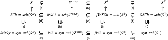
Figure 8: Semantic and syntactic program classes, and selection functions

Let us recall that one of the main goals of this work is the identification and characterization of a syntactic class of programs, based on a syntactic and computable selection function, that:  (a) includes WS programs;  (b) has tractable QA;  (c) is closed under magic-set rewriting (c.f. Figure 1).  It turns out that such a syntactic program class is syn-sch$(\mathcal{S}^{\exists})=$  JWS, of jointly-weakly sticky programs, which we just introduced.  Tractability of QA for JWS and JWSCh will be obtained in Section 4; and closure under magic-set rewriting for JWS will be established in Section 5.

4 Query Answering for Selection-Based Sticky Classes

In this section, we present our chase-based, bottom-up QA algorithm, denoted by ${\sf SChQA}^{\mathcal{S}}$ that is applicable to programs in a semantic class sch$(\mathcal{S})$ or in a syntactic subclass syn-sch$(\mathcal{S})$, where $\mathcal{S}$ is a fixed selection function. Notice that, in general, $\mathcal{S}$ takes a program $\mathcal{P}$ and its EDB $D$, i.e. $\mathcal{S}(\mathcal{P}\cup D)$. However, when $\mathcal{S}$ is syntactic and its result is independent from $D$, we write $\mathcal{S}(\mathcal{P})$. Either way, the selection function returns a set of finite positions, which are used by the algorithm, after it “calls” the selection function. The algorithm relies on the $\mathcal{S}$-stickiness property of the program.

Before presenting the algorithm, in Section 4.3, we discuss, in Section 4.1 and in intuitive terms, the connection between QA and stickiness, for which we use the notions of proof-tree and proof-tree schema. They were introduced in [22] to establish the tractability of QA for (semantically or syntactically) sticky programs. In Section 4.2, that discussion is extended to the case of $\mathcal{S}$-sticky programs, providing the basis for both the QA algorithm under $\mathcal{S}$-sticky programs, and its proof of correctness. The QA algorithm is presented in Section 4.3.

4.1 QA and Stickiness

In this section, when we refer to sticky programs, we mean semantically sticky, in the sense of Definition 5, that characterizes the class SCh of programs with the stickiness property of the chase.

In [22], the authors introduce, for a given, possibly open, conjunctive query over a Datalog⁺ program, the notions of proof-tree and, from the former, that of proof-tree schema. A proof-tree is a finite tree that shows how an answer to the query is inferred. In it, assuming w.l.o.g. that the query is atomic, the instantiated query atom is placed at the root, the leaves are EDB atoms, and a path goes always from a leaf to the root. A proof-tree schema (or pattern) represents the general structures of proof-trees for a given query. The authors in [22] show that, for a query over a sticky program, the height of a proof-tree schema has a fixed upper bound that is independent from the EDB. This provides bounds on the number of chase steps needed to reach an answer, which becomes particularly relevant for proving tractability of QA for sticky programs.

In the following we show these notions and discuss them at the light of some examples of sticky programs (cf. [21] for full details). We do this with the purpose of exploring the extension of those constructs and properties to more relaxed forms of stickiness, as those based on selection functions.

Example 4.1.

Consider the program $\mathcal{P}$ below with EDB $D=\{R(a,b),U(a)\}$ and the CQ  $\mathcal{Q}:P(x,y)$.

$$R(x,y) \rightarrow\exists z\;R(y,z),$$

$$R(x,y),R(y,z) \rightarrow S(x,y,z),$$

$$U(x),S(x,y,z) \rightarrow P(x,y).$$

It is easy to check that this program is syntactically sticky, and then, also semantically sticky, for the given EDB and any other.

The query admits answers w.r.t. $\mathcal{P}\cup D$, namely $(a,b)$, with a proof-tree for it shown in Figure 9(a). The derived query atom, $P(a,b)$, appears at the root, which is an instantiation of the query (a witness for its satisfaction). The leaves are labeled with atoms in $D$. More than one node in the tree might be labeled with the same atom, and each intermediate node (a ground atom) is generated via a rule enforcement, and has as children the atoms that participate in a body of that rule, in particular, in a join.  The proof-tree for $\mathcal{Q}$ in Figure 9(a) is one of the possible subtrees of the chase (also conceived as a tree) that reaches the query predicate and answers the query.

Figure 9(b) shows a proof-tree schema, that represents how a query atom (or a generic root in a proof-tree) can be inferred via the rules in the program when the leaf nodes in the proof schema are mapped to atoms in an EDB. The proof-tree in Figure 9(a) is an instance of this proof-tree schema. $\blacksquare$

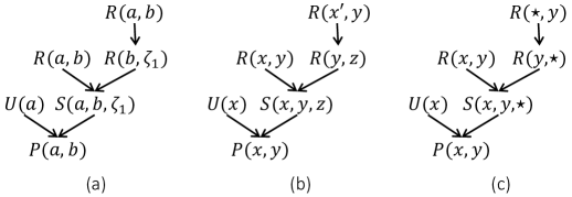
Figure 9: A proof-tree (a) and its schemas (b) and (c) for $\mathcal{Q}$.

Given a program, a query may have different proof-tree schemas, and each proof-tree for an answer is an instantiation of one of them. Every answer to a query over a program has at least one proof-tree.

The variables and atoms in a proof-tree schema have certain properties we need to discuss. Note that a variable $x$ in (an atom in) a proof-tree schema $\mathcal{T}$ is of either one of two types:

1. Variable $x$ appears in two atoms that are not on the same path.

2. If variable $x$ appears in two different atoms, the atoms belong to a same path.

In the proof-tree schema in Figure 9(b), variables $x$ and $y$ fall in case ((I)). Variables $x^{\prime}$ and $z$ fall in case ((II)).

The first property is that a variable falls under case ((I)) only when it appears in a join in the body of a rule that is used to answer the query. In this sense, we sometimes call it “a join variable”. In Figure 9(b), $y$ and $x$ are join variables, because they appear in the join between $R(x,y)$ and $R(y,z)$, and, respectively, in the join between $U(x)$ and $S(x,y,z)$.

The second property is that there is no pair of atoms $A$ and $B$ in any path in $\mathcal{T}$, such that $B$ can be transformed into $A$ by locally renaming its variables of type ((II)). For example, in the right-most path in Figure 9(b), we could not find an atom $R(y,z^{\prime})$, with $z^{\prime}$ of type ((II)), because it could be transformed into $R(y,z)$ (in the same path) by renaming $z^{\prime}$. This property intuitively means a proof-tree schema is a succinct proof for a query answer. For example, if there were $R(y,z)$ and $R(y,z^{\prime})$ in the same path, we could generate a more succinct proof by removing $R(y,z^{\prime})$ and every atom between $R(y,z)$ and $R(y,z^{\prime})$ in the same path, and replacing $z^{\prime}$ in every other atom with $z$. In other words, we can never find two atoms on a same path of the form $T(\bar{x},\bar{y})$, $T(\bar{x},\bar{z})$ (with the variables occupying the same positions in the predicate), with $\bar{x}$ of type (I), and $\bar{y},\bar{z}$ of type (II).

Using this succinctness property, and the fact that the program’s schema is fixed, one can show that the number of atoms in any path in a proof-tree schema only depends on the number of variables of type ((I)) [22, Lemma 3.3]. We can see this by replacing in a proof-tree schema every variable of type ((II)) by a place holder, say $\star$, which is allowed by the fact that these variables do not appear in any other paths, and can be locally replaced. The replacements are shown in Figure Figure 9(c).   The maximum number of atoms in a path is bounded above by the all the ways to fill program predicates with variables of type ((I)) plus $\star$.

Now, we proceed to analyze variables of type (I) in a proof-tree schema under the assumption that the program is sticky. Notice that the discussion of variables of type (II) above does not make any stickiness assumption.

As mentioned at the beginning of this section, stickiness guarantees that the height of a proof-tree (and a proof-tree schema) for every answer to a CQ has an upper bound that is fixed, independent from the EDB. Let us elaborate on this. Stickiness implies that the variables of type ((I)) are propagated all the way down to the root, and, as a consequence, the number of type ((I)) variables in a proof-tree schema is bounded above by the number of arguments in the query.

For illustration, in Example 4.1 and the proof-tree schema in Figure 9(b); variables $x$ and $y$, both of type ((I)), appear in the root atom, which has only two arguments. Therefore, the number of type ((I)) variables cannot be larger than two. Since the number of atoms in a path in a proof-tree schema only depends on the number of variables of type ((I)), we can conclude that the total number of atoms in any path in the proof-tree schema of a SCh program has a fixed upper bound (which is provided in [22, Lemma 3.3]).

In Example 4.3, we will see a non-sticky program and a query for which a proof-tree schema has a number of type ((I)) variables that depends on the size of the EDB.

As a result of this discussion, we can claim that for an answer to a query over a SCh program, the height of a proof-tree schema has a fixed upper bound. This implies that QA can be done over an initial portion of the chase of the sticky program, with atoms that are obtained after a fixed number of chase steps. The idea behind the QA algorithm for sticky programs in SCh  consists in exploring a sufficiently large portion of the chase that covers the proof-tree.  As we will see in the next section, this kind of analysis of QA on sticky programs and their properties can be generalized to the case of $\mathcal{S}$-sticky programs.

4.2 QA and $\mathcal{S}$-stickiness

As we saw in the previous section, for sticky programs, the height of a proof-tree schema has an upper bound that is fixed and independent from the EDB. It turns out that $\mathcal{S}$-sticky programs enjoy a similar property, with the difference that the upper bound is a fixed number that depends on $\mathcal{S}$ and the EDB.

In order to show this, consider a proof-tree schema $\mathcal{T}$ for a query over a program $\mathcal{P}\cup D$. Given a selection function $\mathcal{S}$, the variables of type ((I)) (of the previous section) in $\mathcal{T}$ can be divided into two sub-types:

• Variables that appear at least once in a position in $\mathcal{S}(\mathcal{P}\cup D)$, and

• Variables that do not appear in these positions.

Example 4.2.

Consider a program $\mathcal{P}\cup D$, with $\mathcal{P}$ containing only the rule $R(x,y),R(y,z)\rightarrow R(x,z)$; $D=\{R(a,c),R(c,d),R(d,b)\}$, and the BCQ query, $\mathcal{Q}:R(a,b)$, asking if $R(a,b)$ is true. The program is not not in SCh, because the value $c$ that replaces the join variable $y$ does not appear in $R(a,d)$.

Figures 10(b) and  11(b) show the proof-trees and the proof-tree schemas for $\mathcal{Q}$.  In them, variable $x,w$ are of type (II); and variables $y,z$ are of type (I), because they appear in more than one branch of the trees. The subtypes, ((I.1)) or ((I.2)), the latter belong to depend on the selection function $\mathcal{S}$.

Consider $\mathcal{S}=\mathcal{S}^{\it rank}$. In this case, $\mathcal{S}^{\it rank}$ contains every position (of predicates) in $\mathcal{P}$. Then, variables $y,z$ in Figure 11(b) are of sub-type ((I.1)), because they appear in $\mathcal{S}^{\it rank}$-finite positions. In contrast, notice that for $\mathcal{S}=\mathcal{S}^{\bot}=\emptyset$, these two variables are of sub-type ((I.2)). $\blacksquare$

For an $\mathcal{S}$-sticky program, the variables of sub-type ((I.2)) will appear in the root query atom, and their occurrences are restricted by the query (the same argument as for stickiness above applies to this case). The number of variables of sub-type ((I.1)) is limited by the finitely many values in $\mathcal{S}$-finite positions (since the number of values that these variables take is also limited). Therefore, the number of atoms in any path in a proof-tree schema depends on the query, the program’s schema and also the number of values that can appear in $\mathcal{S}$-finite positions. This last number depends on the EDB.

As a consequence, we obtain that for a program in sch$(\mathcal{S})$, the height of a proof-tree schema for a query depends on program’s schema, the query, and the number of values in $\mathcal{S}$-finite positions, which in turn depends on the size of the program’s EDB. This is illustrated in Example 4.3 right below.

Example 4.3.

Consider $\mathcal{P}$, $D$ and $\mathcal{Q}$ of Example 4.2; and also the EDB $D^{\prime}=\{R(a,c),R(c,b)\}$. The programs $\mathcal{P}\cup D$ and $\mathcal{P}\cup D^{\prime}$ are not in SCh, but they are in sch$(\mathcal{S}^{\it rank})$.

The heights of the proof-trees and proof-tree schemas of $\mathcal{Q}$ w.r.t. $\mathcal{P}\cup D$ and $\mathcal{P}\cup D^{\prime}$ in Figures 10 and  11 are $3$ and $2$, resp., which means the heights depend on the size of the EDBs. $\blacksquare$

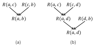
Figure 10: The proof-trees of $\mathcal{Q}$

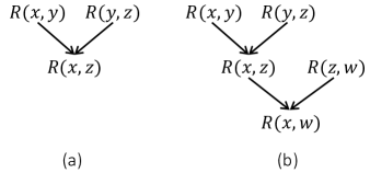
Figure 11: The proof-tree schemas of $\mathcal{Q}$

The discussion in this section shows that, although the chase instance of a program in ${\it sch}(\mathcal{S})$ may be infinite, QA can be done on a fixed initial portion of it. This is because the height of a proof-tree schema, for any answer, has a fixed upper bound, which may depend on the size of the EDB. In the rest of this section we will make these properties precise. In Section 4.3, they will be applied to design a QA algorithm for programs in sch($\mathcal{S}$). It will be based on a query-dependant chase procedure that generates this finite portion, for which the next lemma provided an upper bound. Its proof relies on the considerations we have made so far in this section.

Proposition 6.

Consider a CQ $\mathcal{Q}$ over a program $\mathcal{P}\cup D$ in sch$(\mathcal{S})$. Let $\mathcal{T}$ be a proof-tree schema for an answer $t\in\mathcal{Q}(\mathcal{P}\cup D)$. An upper bound for the height of $\mathcal{T}$ is $p\times(s+q+1)^{r}$, where $p$ is the number of program predicates, $r$ is their maximum arity, $s$ is the number of nulls appearing in positions in $\mathcal{S}(\mathcal{P}\cup D)$ during the chase of the program, and $q$ is the number of variables in $\mathcal{Q}$. $\blacksquare$

Proof:  We find an upper bound on the height of $\mathcal{T}$ by computing the maximum number of atoms in any path $\beta$ from a leaf node to the root of $\mathcal{T}$. The number of variables of sub-type ((I.2)) in $\beta$ is at most $q$. This is because $\mathcal{P}\cup D$ is in sch$(\mathcal{S})$ which means these variables also appear in $\mathcal{Q}$. The number of variables of sub-type ((I.1)) in $\beta$ is $s$, which is the number of values that these variables take. As discussed in Section 4.1, to count the number of atoms in $\beta$, we can replace every variable of type ((II)) by a place holder, $\star$, because these variables do not appear in any other paths. Therefore, the number of possible terms in the atoms in any path of $\mathcal{T}$ is $s+q+1$. Since there are $p$ predicate names with maximum arity $r$ in $\mathcal{P}$, we can generate at most $p\times(s+q+1)^{r}$ atoms with these terms, which will be the upper bound on the length of $\beta$ and also the height of $\mathcal{T}$. $\blacksquare$

Proposition 6 is generic for selection functions $\mathcal{S}$ and specifies an upper bound on the height of the proof-tree schema for programs in a class determined by sch$(\mathcal{S})$. The upper-bound depends on $\mathcal{S}$ and $s$. With a more general $\mathcal{S}$, i.e. that returns more positions, the class of programs sch$(\mathcal{S})$ is more general and contains more programs. At the same time, the value of $s$ and the upper-bound $(s+q+1)^{r}$ increase since $s$ counts values in possibly more positions. This means for programs in a more general class sch$(\mathcal{S})$, the height of a proof-tree schema can be larger, and the proof may become more complex. The extreme cases are sch$(\mathcal{S}^{\bot})$ and sch$(\mathcal{S}^{\top})$. In ${\it SCh}={\it sch}(\mathcal{S}^{\bot})$, which is the smallest semantic class, $s=0$, and the upper bound on proof-tree schemas takes the smallest value. For ${\it GSCh}={\it sch}(\mathcal{S}^{\top})$, which is the most general semantic class, $s$ is maximum, and the upper bound on proof-tree schemas takes the largest possible value. Regarding QA over programs in sch$(\mathcal{S})$, this proposition implies that for more general classes of sch$(\mathcal{S})$, the chase has to run more steps to cover proofs with larger height.

From the definition of $\mathcal{S}$-finite position (c.f. Definition 1), $s$ in Proposition 6 is indeed finite. Neither that definition nor the Proposition give us an upper bound for $s$. For each specific selection function, one has to determine that bound, if possible. However, for some of them we know such a bound.

Lemma 1.

For a Datalog⁺ program $\mathcal{P}\cup D$, the number $s$ of nulls appearing in positions in $\mathcal{S}^{\it rank}(\mathcal{P})$ is polynomially bounded in the size of $D$. Actually, the number of values (constants or nulls) in positions of $\mathcal{S}^{\it rank}(\mathcal{P})$ during the chase is $O(n^{v\times k})$, where $n$ is the number of constants in $D$, $v$ is the maximum number of variables in a rule in $\mathcal{P}$, and $k$ is the maximum rank of the positions in $\mathcal{S}^{\it rank}$ (c.f. Section 2.3.1). $\blacksquare$

The proof of Lemma 1 is implicit in that of [27, Theorem 3.9], which establishes when $\mathcal{P}$ is WA  that the number of values in the chase of $\mathcal{P}\cup D$ is $O(n^{v\times k})$. Notice that Lemma 1 does not require the program to belong to WA or ${\it sch}(\mathcal{S}^{\it rank})$. This is because the lemma is limited to the positions of $\mathcal{S}^{\it rank}(\mathcal{P})$, unlike [27, Theorem 3.9] that does not restrict the positions. Also notice that in this lemma we use $\mathcal{S}^{\it rank}(\mathcal{P})$, and not $\mathcal{S}^{\it rank}(\mathcal{P}\cup D)$, because $\mathcal{S}^{\it rank}$ is a syntactic selection function that depends only on the program without the EDB. For the same reason, we use $\mathcal{S}^{\exists}(\mathcal{P})$ in Lemma 2 below, where we establish a similar upper bound for $\mathcal{S}^{\exists}$. This upper bound depends on $k_{\exists}$ that is the maximum $\exists$-rank of positions in $\mathcal{S}^{\exists}$ (c.f. Definition 7).

Lemma 2.

For a Datalog⁺ program $\mathcal{P}\cup D$, the number of distinct values (constants or nulls) in ${\it chase}(\mathcal{P}\cup D)$ that appear at least once in a position in $\mathcal{S}^{\exists}(\mathcal{P})$ is polynomially bounded above by the size of $D$; actually by $O(n^{v\times k_{\exists}})$, where $n$ is the number of constants in $D$, $v$ is the maximum number of variables in a rule in $\mathcal{P}$, and $k_{\exists}$ is the maximum $\exists$-rank of a position in $\mathcal{S}^{\exists}(\mathcal{P})$. $\blacksquare$

Proof:  For the proof, we first partition the positions in $\mathcal{P}$ into $\Pi_{0},\Pi_{1},...,\Pi_{k_{\exists}}$, where $\Pi_{i}$ is the set of positions with the $\exists$-rank $i$, and $k_{\exists}$ is the maximum $\exists$-rank, which is bounded by the total number of positions in $\mathcal{P}$. Let $d_{i}$ be the number of values that appear in the positions of $\Pi_{i}$ during the chase of $\mathcal{P}\cup D$. We prove by induction on $i$ that $d_{i}$ is polynomial in $n$, i.e. the number of constants in $D$:

Base case: $d_{0}$ is $O(n)$ with $n$ because there is only constants from $D$ in positions of $\Pi_{0}$.

Inductive step: If for every $j<i$, $d_{j}$ is a polynomial function $P_{j}(n)$, then $d_{i}$ is also a polynomial function $P_{i}(n)$. To prove this inductive step, consider the following three cases for a value, constant or null, that appears in a position of $\Pi_{i}$: (a) it is a constant that appears in a position of $\Pi_{i}$ in an atom in $D$, (b) it is a null or a constant that is copied from a position of $\Pi_{j}$ to a position in $\Pi_{i}$, or (c) it is a null that is invented by an $\exists$-variable $z$ in a position in $\Pi_{i}$. An upper bound for the number of terms in (a) is $n$. By the inductive hypothesis, the number of values in (b) is at most $K_{i}(n)=P_{i-1}(n)+P_{i-2}(n)+...+P_{0}(n)$ which is a polynomial function in $n$. For (c), any such variable $z$ appears at the end of at least one path of length $i$ in the EDG of $\mathcal{P}$. Let $\sigma$ be a rule containing such a $\exists$-variable, $z$. The values in ${\it body}(\sigma)$ are in positions with $\exists$-rank less than $i$. Let $v$ be the maximum number of variables in the body of any rule in $\mathcal{P}$. Then, $\sigma$ can invent $K_{i}(n)^{v}$ new values in the positions of $\Pi_{i}$ since each variable can be replaced with $K_{i}(n)$ values from $\Pi_{j}$. If there are at most $w$ rules in $\mathcal{P}$ and each rule can have at most $r$ existential variables, which is the maximum arity of the predicates in $\mathcal{P}$, then there are at most $w\times r\times K_{i}(n)^{v}$ distinct values in the positions of $\Pi_{i}$ which is polynomial in $n$. Putting these together, $d_{i}$ is at most $n+K_{i}(n)+w\times r\times K_{i}(n)^{v}$. Applying the recursive definition of $K_{i}$, we can conclude that $P_{i}(n)=O(n^{i.v})$, and for $i={k_{\exists}}$, $d_{k_{\exists}}$ is a polynomial function $P_{k_{\exists}}(n)=O(n^{{k_{\exists}}.v})$. $\blacksquare$

The proof of Lemma 2 is based on the proof of Theorem 3.9 in  [27]. The main difference is that Lemma 2 is about positions in $\mathcal{S}^{\exists}(\mathcal{P})$, whereas the theorem in [27] is about WA programs, and positions in $\mathcal{S}^{\it rank}(\mathcal{P})$. We provide the complete proof of Lemma 2 here to make it clear how $\mathcal{S}^{\exists}(\mathcal{P})$ positions are used in the proof.  Notice that, similar to Lemma 1, Lemma 2 does not require $\mathcal{P}\cup D$ to be in WA or sch$(\mathcal{S})$, and it can be any Datalog⁺ program.

From Proposition 6 we conclude that, when the number of null values in $\mathcal{S}$-finite positions is polynomially bounded above by the size of $D$, then the height of a proof-tree schema is also polynomially bounded above by the size of $D$. Now, from Lemmas 1 and 2, we conclude that this is the case for $\mathcal{S}^{\it rank}$-finite positions and $\mathcal{S}^{\exists}$-finite positions, respectively. For the two associated program classes, Corollary 2 below gives us explicit upper bounds for the height of proof-tree schemas.

Corollary 2.

For a CQ $\mathcal{Q}$ over a program $\mathcal{P}\cup D$ in sch$(\mathcal{S}^{\it rank})$ or sch$(\mathcal{S}^{\exists})$, the height of a proof-tree schema for an answer in $\mathcal{Q}(\mathcal{P}\cup D)$ is polynomially bounded above by the size of $D$. More precisely, an upper bound is $O(n^{v\times k\times r})$ for $\mathcal{S}=\mathcal{S}^{\it rank}$, and $O(n^{v\times{k_{\exists}}\times r})$ for $\mathcal{S}=\mathcal{S}^{\exists}$. $\blacksquare$

Theorem 4.1 concludes our discussion about the connection between QA and $\mathcal{S}$-stickiness, and it summarizes the results in Proposition 6, Lemma 2, and Corollary 2. While we state the theorem for semantic program classes sch($\mathcal{S}$), the same statement holds for the associated syntactic sub-classes syn-sch$(\mathcal{S})$.

Theorem 4.1.

Consider a program $\mathcal{P}\cup D$ in sch($\mathcal{S}$). The following holds:

1. If the selection function $\mathcal{S}$ is computable, then QA over $\mathcal{P}\cup D$ is decidable.

2. If the computation of $\mathcal{S}(\mathcal{P}\cup D)$ is tractable in the size of $D$, and the number of values (constants or nulls) that appear in the positions in $\mathcal{S}(\mathcal{P}\cup D)$ during the chase of $\mathcal{P}\cup D$ is polynomially bounded above by the size of $D$, then QA over $\mathcal{P}\cup D$ is also tractable in the size of $D$.

3. In particular, when $\mathcal{S}=\mathcal{S}^{\exists}$ or $\mathcal{S}=\mathcal{S}^{\it rank}$, QA over $\mathcal{P}\cup D$ can be done in polynomial time in the size of $D$.

Proof:  (a) follows from Proposition 6 that gives an upper-bound for the height of a proof-tree schema for an answer to a CQ over a program in sch($\mathcal{S}$). This means that the proof can be mapped to a fixed initial portion of the chase. Therefore, QA is decidable for sch($\mathcal{S}$). Now, (b) follows from Proposition 6 and the fact that $s$, and then also the upper bound $p\times(s+q+1)^{r}$, are polynomially bounded above in the size of EDB. Finally, (c) follows from (b), Corollary 2, and the fact that computing $\mathcal{S}(\mathcal{P}\cup D)$ for $\mathcal{S}=\mathcal{S}^{\exists}$ or $\mathcal{S}=\mathcal{S}^{\it rank}$ can be done in constant time w.r.t. the size of EDB. The last claim holds because $\mathcal{S}^{\exists}$ and $\mathcal{S}^{\it rank}$ are syntactic functions, and then, independent from the EDB. $\blacksquare$

In this section, we provided a comprehensive complexity analysis of QA over programs in ${\it sch}(\mathcal{S})$. We showed $\mathcal{S}$-stickiness for a computable selection function $\mathcal{S}$ makes QA decidable, and under certain conditions on $\mathcal{S}$, stated in Theorem 4.1(b), QA becomes tractable. In the next section, we provide a QA algorithm based on the results in this section. It works for the general ${\it sch}(\mathcal{S})$ class, while its runtime depends on the selection function $\mathcal{S}$.

4.3 The ${\sf SChQA}^{\mathcal{S}}$ Algorithm

${\sf SChQA}^{\mathcal{S}}$ is a QA algorithm for Datalog⁺ programs in ${\it sch}(\mathcal{S})$, where $\mathcal{S}$ maps programs with their EDBs to sets of finite positions (but not necessarily all finite positions). The algorithm is parameterized by (or calls as a subroutine) the selection function $\mathcal{S}$, which can be computed when it is computable or seen as an oracle, otherwise. The algorithm accepts as input a program $\mathcal{P}\cup D\in{\it sch}(\mathcal{S})$ and a CQ $\mathcal{Q}$, and returns $\mathcal{Q}(\mathcal{P}\cup D)$. The query may contain free variables.

The algorithm runs first what we call the $\langle\mathcal{Q},\mathcal{S}\rangle$-chase procedure, which is a modified version of the classic chase with $\mathcal{P}\cup D$, that now generates an initial, finite, and $\mathcal{Q}$-dependent portion of the (classic) chase instance of $\mathcal{P}\cup D$. This portion of the chase includes the ground atoms in the proof-trees for the answers to query $\mathcal{Q}$. Furthermore, $\langle\mathcal{Q},\mathcal{S}\rangle$-chase differs from the classic chase only in that it considers a more restrictive condition for the application of a chase step, which guarantees termination.  After running the $\langle\mathcal{Q},\mathcal{S}\rangle$-chase, ${\sf SChQA}^{\mathcal{S}}$ computes the answers to $\mathcal{Q}$ over this finite portion of the chase, as a regular query posed to a finite instance.

In order to define the $\langle\mathcal{Q},\mathcal{S}\rangle$-chase, we need first the notions of homomorphic atoms and freezing a null. (C.f. Section 2.1 for the definition of homomorphism.)

Definition 9 ($\Pi$-homomorphism and freezing nulls).

Let $\mathcal{R}$ be a program schema, and $\Pi$ a set of predicate positions.  (a) Given two ground atoms $A$ and $B$, i.e. containing only constants or nulls, $A$ is $\Pi$-homomorphic to $B$ if there is a homomorphism $h:\{A\}\rightarrow\{B\}$ (in particular, the atoms share the predicate and $h(A)=B$), and $h$ is the identity on terms in positions in $\Pi$.

(b) Freezing a null $\zeta\in\Gamma^{N}$ in an instance $I$ means replacing every occurrence of $\zeta$ in $I$ with a constant $\zeta^{f}\in\Gamma^{C}$ (assuming the set of constants is extended with these fresh constants that do not appear anywhere in the initial EDB or the program).   $\blacksquare$

Notice that $A$ is homomorphic to $B$ if $A$ is $\Pi$-homomorphic to $B$ with $\Pi=\emptyset$ or $\Pi$ does not contain positions of $A$. Freezing a null in an atom $A$ means freezing the null in instance $\{A\}$.

Example 4.4.

The ground atom $S(a,\zeta,\zeta)$ is $\{S[1]\}$-homomorphic to $S(a,b,b)$, with $h=\{a\mapsto a,\zeta\mapsto b\}$, but it is not $\{S[2]\}$-homomorphic.  Atom $S(a,b,b)$ is not $\{S[1]\}$-homomorphic to $S(a,\zeta,\zeta)$. Atom $S(a,\zeta,\zeta)$ is not homomorphic to $S(a,b,c)$.

Freezing the null $\zeta$ in $S(a,\zeta,\zeta)$ means, in practical terms, treating $\zeta$ in it as a constant. This may have an impact on possible homomorphisms that involve the atom. For example, after replacing $S(a,\zeta,\zeta)$ by $S(a,\zeta^{f},\zeta^{f})$, with $\zeta^{f}$ a constant, $S(a,\zeta^{f},\zeta^{f})$ is not homomorphic to $S(a,b,b)$ anymore, because $\zeta^{f}$ and $b$ are (syntactically) different constants. $\blacksquare$

Definition 10 (Applicable rule-assignment pair).

Consider a Datalog⁺ program $\mathcal{P}\cup D$ and an instance $I\supseteq D$. A rule-assignment pair $(\sigma,\theta)$, with $\sigma\in\mathcal{P}$, is $\mathcal{S}(\mathcal{P}\cup D)$-applicable over $I$ if:  (a) $\theta({\it body}(\sigma))\subseteq I$; and (b) there is an assignment $\theta^{\prime}$ that extends $\theta$, maps the $\exists$-variables of $\sigma$ into nulls that do not appear in $I$ (i.e. they are fresh nulls), and $\theta^{\prime}({\it head}(\sigma))$ is not $\mathcal{S}(\mathcal{P}\cup D)$-homomorphic to any atom in $I$. $\blacksquare$

When $\mathcal{S}$ and $\mathcal{P}\cup D$ are clear from the context, we will simply say “the rule is applicable”. Typically, $I$ will be a finite portion of ${\it chase}(\mathcal{P},D)$. For an instance $I$ and a program $\mathcal{P}$, we can systematically compute the applicable rule-assignment pairs by first finding $\sigma\in\mathcal{P}$ for which ${\it body}(\sigma)$ is satisfied by $I$. That gives an assignment $\theta$ for which $\theta({\it body}(\sigma))\in I$. Next, we construct a $\theta^{\prime}$ according to Definition 10, and we check for each atom in $I$ that there is no $\mathcal{S}(\mathcal{P}\cup D)$-homomorphism from $\theta^{\prime}({\it head}(\sigma))$.

Example 4.5.

Consider a program $\mathcal{P}\cup D$ with $D=\{P(a,b)\}$ and the rule:

$$\sigma:P(x,y)\rightarrow\exists zP(y,z).$$ (16)

Also consider instance $I=D\cup\{P(b,\zeta)\}$, and the selection function $\mathcal{S}^{\it rank}$. There is no finite position according to the selection function, i.e. $\mathcal{S}^{\it rank}(\mathcal{P})=\emptyset$. The rule-assignment $(\sigma,\theta)$ with $\theta=\{x\mapsto b,y\mapsto\zeta\}$ is not applicable over $I$, because any extension $\theta^{\prime}({\it head}(\sigma))=P(\zeta,\zeta^{\prime})$ is $\emptyset$-homomorphic to $P(b,\zeta)\in I$.

Freezing $\zeta$ in $I$ by replacing it with the constant $\zeta^{f}$ makes $(\sigma,\theta)$ applicable since a head extension of the form $P(\zeta^{f},\zeta^{\prime})$ is not $\emptyset$-homomorphic to any of the atoms $P(a,b)$ or $P(b,\zeta^{f})$ in $I$. $\blacksquare$

The technique of freezing nulls was first used in [33] for QA over shy Datalog⁺ programs. The modified chase procedure we are about to introduce is based on the parsimonious chase for Shy Programs [33].

We present now our new chase procedure, $\langle\mathcal{Q},\mathcal{S}\rangle$-chase. It is a modified chase that produces a finite instance. $\langle\mathcal{Q},\mathcal{S}\rangle$-chase appeals to the notions of freezing nulls and $\Pi$-homomorphism of Definition 9, and rule applicability of Definition 10.

Definition 11.

Given a CQ $\mathcal{Q}$ over a program $\mathcal{P}\cup D$ and a selection function $\mathcal{S}$, $\langle\mathcal{Q},\mathcal{S}\rangle\mbox{-}{\it chase}(\mathcal{P}\cup D)$ is the instance $I$ that is obtained from $D$ after iteratively applying the following steps, with $I$ initially equal to $D$: (This is the $\langle\mathcal{Q},\mathcal{S}\rangle$-chase procedure.)

• Step 1. For every $\mathcal{S}(\mathcal{P}\cup D)$-applicable rule-assignment pair $(\sigma,\theta)$ over $I$, add $\theta^{\prime}({\it head}(\sigma))$ to $I$ (c.f. Definition 10). Go to Step 11 if all the applicable pairs are applied, producing a possibly extended instance $I$.

• Step 2. (resumption step) Freeze every null in $I$ and go to Step 11. Apply resumption $M_{\mathcal{Q}}$ times, where $M_{\mathcal{Q}}$ is the number of $\exists$-variables in $\mathcal{Q}$. $\blacksquare$

Notice that this chase does not have anything like an “unfreezing” step. What was frozen stays frozen.

So as the usual the chase procedure, the $\langle\mathcal{Q},\mathcal{S}\rangle$-chase procedure applies a pair of rule-assignment only once. Furthermore, the $\langle\mathcal{Q},\mathcal{S}\rangle$-chase procedure applies rule-assignments in the same order as the usual chase procedure. The main difference between $\langle\mathcal{Q},\mathcal{S}\rangle$-chase and the latter resides in the applicability condition in Step 11 that uses $\mathcal{S}$ to check $\mathcal{S}(\mathcal{P}\cup D)$-homomorphism. This requires the computation of the $\mathcal{S}(\mathcal{P}\cup D)$ positions. For computability and complexity analysis, we assume this computation is done at once by an oracle that runs $\mathcal{S}$ in constant time w.r.t. $D$.

The $\langle\mathcal{Q},\mathcal{S}\rangle$-chase procedure is a partial chase procedure in the sense that the $\langle\mathcal{Q},\mathcal{S}\rangle$-chase instance is a subset of the usual chase instance modulo renaming nulls. This is because any pair of rule-assignment that is applicable in the $\langle\mathcal{Q},\mathcal{S}\rangle$-chase procedure is also applicable in the usual chase; the applicability condition in $\langle\mathcal{Q},\mathcal{S}\rangle$-chase extends the applicability condition in the usual chase.

Example 4.6.

Consider a query $\mathcal{Q}(x):\exists y\;R(x,y)$ over a program $\mathcal{P}\cup D$ with rules as below, and the EDB $D=\{P(a,b)\}$.

$$\sigma_{1}: \hskip 28.45274ptP(\hat{x},\hat{y})~{}\rightarrow~{}\exists z\;P(y,z),$$

$$\sigma_{2}: \hskip 28.45274ptP(x,y),P(y,\hat{z})~{}\rightarrow~{}\;R(x,y).$$

The program is sticky, because there is no repeated marked variable in a body. Then, it is in sch$(\mathcal{S}^{\bot})$, i.e. $\mathcal{S}=\mathcal{S}^{\bot}$. As a consequence, the positions we have to consider for rule applicability are those in $\mathcal{S}^{\bot}(\mathcal{P})=\emptyset$.

The $\langle\mathcal{Q},\mathcal{S}\rangle$-chase runs as follows. It starts from $I:=D$. The pair $(\sigma_{1},\theta_{1})$ with $\theta_{1}:x\!\mapsto\!a,y\!\mapsto\!b$ is applicable; and the procedure adds $P(b,\zeta_{1})$ to $I$. The next applicable pair is $(\sigma_{2},\theta_{2})$ with $\theta_{2}:x\!\mapsto\!a,y\!\mapsto\!b,z\!\mapsto\!\zeta_{1}$ and adds $R(a,b)$ to $I$. The pair $(\sigma_{1},\theta_{3})$ with $\theta_{3}:x\!\mapsto\!b,y\!\mapsto\!\zeta_{1}$ is not applicable because it generates $P(\zeta_{1},\zeta_{2})$ that is homomorphic to $P(a,b)$.

The query has an $\exists$-variables $y$, $M_{\mathcal{Q}}=1$. So, the procedure continues with Step 11 of Definition 11, by freezing $\zeta_{1}$, i.e. replacing it by the constant $\zeta_{1}^{f}$.

As a result, $(\sigma_{1},\theta_{3})$ becomes applicable, and adds $P(\zeta_{1}^{f},\zeta_{2})$, that consequently makes $(\sigma_{1},\theta_{4})$, with $\theta_{4}:x\!\mapsto\!b,y\!\mapsto\!\zeta_{1}^{f},z\!\mapsto\!\zeta_{2}$, applicable, and adds $R(b,\zeta_{1}^{f})$. Note that, after $\zeta_{1}$ is frozen, $(\sigma_{2},\theta_{2})$ is not applied again.

The procedure stops since there is no applicable pair that is not already applied, and the only allowed resumption is applied. The result of the procedure is $I=D\cup\{P(b,\zeta_{1}^{f}),R(a,b),P(\zeta_{1}^{f},\zeta_{2}),R(b,\zeta_{1}^{f})\}$.

The answer to $\mathcal{Q}$ over $I$ contains $a$ and $b$, i.e. $\mathcal{Q}(I)=\{a,b\}$. We will show in Theorem 4.2 that this is equal to the answer from the program $\mathcal{P}\cup D$, i.e. $\mathcal{Q}(\mathcal{P}\cup D)=\mathcal{Q}(I)$, which means the $\langle\mathcal{Q},\mathcal{S}\rangle$-chase can be used for QA over the program $\mathcal{P}\cup D$. $\blacksquare$

Example 4.6 shows running the $\langle\mathcal{Q},\mathcal{S}\rangle$-chase procedure with $\mathcal{S}=\mathcal{S}^{\bot}$ that determines the simplest (or better, smaller) syntactic (sticky) and semantic (sch$(\mathcal{S}^{\bot})$) program classes. This allowed us to easily illustrate the applicability condition, and the resumption step. In the next example, we show the $\langle\mathcal{Q},\mathcal{S}\rangle$-chase procedure with other selection functions, to show the impact of $\mathcal{S}$ on the procedure, and QA.

Example 4.7.

Consider the program $\mathcal{P}\cup D$ with rules as below and EDB $D=\{P(a,b),P(b,c),V(b),V(c)\}$, and the query $\mathcal{Q}(x):U(x)$.

$$\sigma_{1}: \hskip 28.45274ptP(x,y),V(y)~{}\rightarrow~{}\exists z\;P(y,z),$$

$$\sigma_{2}: \hskip 28.45274ptP(x,y),P(y,z)~{}\rightarrow~{}\;U(x).$$

We consider below two different selection functions. In the first case, the program does belong to the associated semantic program class, but it the second, it does not.

(a) If $\mathcal{S}=\mathcal{S}^{\exists}$, $\mathcal{S}(\mathcal{P})$ contains every position in $\mathcal{P}$, because the EDG of $\mathcal{P}$ — a simple graph that we do not show as it only contains one node representing $z$ in $\sigma_{1}$ and it does not have any edges — is cycle-free, and therefore all the positions have finite $\exists$-rank. The program is trivially in sch$(\mathcal{S})$.

The $\langle\mathcal{Q},\mathcal{S}\rangle$-chase runs as follows. It starts from $I:=D$. The pairs $(\sigma_{1},\theta_{1})$, with $\theta_{1}:x\!\mapsto\!b,y\!\mapsto\!c$, and $(\sigma_{2},\theta_{2})$, with $\theta_{2}:x\!\mapsto\!a,y\!\mapsto\!b,z\!\mapsto\!c$, are applicable. With them, the procedure adds $P(c,\zeta_{1})$ and $U(a)$ to $I$. Notice that the pair $(\sigma_{1},\{x\mapsto a,y\mapsto b\})$ is not applicable because of $P(b,c)$.

The next applicable pairs are $(\sigma_{1},\theta_{3})$, with $\theta_{3}:x\!\mapsto\!c,y\!\mapsto\!\zeta_{1}$, and $(\sigma_{2},\theta_{4})$, with $\theta_{4}:x\!\mapsto\!b,y\!\mapsto\!c,y\!\mapsto\!\zeta_{1}$. They add $P(\zeta_{1},\zeta_{2})$ and $U(b)$ to $I$. Finally, the pair $(\sigma_{2},\theta_{5})$, with $\theta_{5}:x\!\mapsto\!c,y\!\mapsto\!\zeta_{1},z\!\mapsto\!\zeta_{2}$, becomes applicable, and adds $U(c)$ to $I$.

There are no more applicable pairs, and we continue with Step 11. In this case, the $\langle\mathcal{Q},\mathcal{S}\rangle$-chase chase does not apply any resumptions since $\mathcal{Q}$ does not have any $\exists$-variables. The final instance is $I=D\cup\{P(c,\zeta_{1}),U(a),U(b),P(\zeta_{1},\zeta_{2}),U(c)\}$. The instance $I$ correctly answers $\mathcal{Q}$, i.e. $\mathcal{Q}(\mathcal{P}\cup D)=\mathcal{Q}(I)=\{a,b,c\}$.

(b) Now let us consider $\mathcal{S}=\mathcal{S}^{\it rank}$, that, in general, determines a smaller class of programs than $\mathcal{S}^{\exists}$. In this case, $\mathcal{S}^{\it rank}(\mathcal{P}\cup D)=\{V[1]\}$. More specifically, the DG of $\mathcal{P}$ in Figure 12 includes cycles with special edges. From this, $P[1],P[2]$ and $U[1]$ have infinite rank: these cycles create paths of infinite size that end at these positions. However, there is no such paths ending with $V[1]$, and therefore, the rank of $V[1]$ is $0$. The program does not belong to sch$(\mathcal{S}^{\it rank})$.

We can see this more clearly as follows: If during the chase of $\mathcal{P}\cup D$ and while applying $\sigma_{2}$, the value $b$ participates in a join, $P(a,b)\wedge P(b,c)$, in positions $P[2],P[1]$, both with infinite rank, and $b$ does not appear in the result $U(a)$; and then, it does not “stick”.

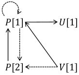
Figure 12: The DG  of $\mathcal{P}$

If, despite of this, we run the $\langle\mathcal{Q},\mathcal{S}\rangle$-chase procedure, it generates the instance $I=D\cup\{P(c,\zeta_{1}),U(a),U(b)\}$, after applying $(\sigma_{1},\theta_{1})$, $(\sigma_{2},\theta_{2})$ and $(\sigma_{2},\theta_{4})$. Notice that $(\sigma_{1},\theta_{3})$ is not applicable, because $P(\zeta_{1},\zeta_{2})$ is $\mathcal{S}^{\it rank}(\mathcal{P})$-homomorphic to existing atoms in $I$, e.g. $P(c,\zeta_{1})$. In this case, when $\mathcal{S}=\mathcal{S}^{\it rank}$, the instance $I$ does not give all the answers to $\mathcal{Q}$: $\mathcal{Q}(\mathcal{P}\cup D)=\{a,b,c\}$, but $\mathcal{Q}(I)=\{a,b\}$.

This example shows that the $\langle\mathcal{Q},\mathcal{S}\rangle$-chase procedure returns an instance that may generate incomplete answers if the program is not in sch$(\mathcal{S})$. $\blacksquare$

As the example above illustrates, given a program $\mathcal{P}\cup D$ and a query $\mathcal{Q}$, we can choose any selection function $\mathcal{S}$ to apply the QA procedure. However, there is no guarantee that the result will be correct. Actually, as we will see in Section 4.4, the $\langle\mathcal{Q},\mathcal{S}\rangle$-chase can be guaranteed to be correct for QA if only if $\mathcal{P}\cup D$ is in sch$(\mathcal{S})$.  Still, there might be more than one (correct) selection function to use. For example, if the program belongs to sch$(\mathcal{S}^{\bot})$, then it also belongs to sch$(\mathcal{S}^{\exists})$. Both $\langle\mathcal{Q},\mathcal{S}^{\bot}\rangle$-chase and $\langle\mathcal{Q},\mathcal{S}^{\exists}\rangle$-chase can be correctly used for QA with the program. In Theorem 4.2 we will show they run in PTIME.

Having introduced the $\langle\mathcal{Q},\mathcal{S}\rangle$-chase procedure, we are not in position to formally present the ${\sf SChQA}^{\mathcal{S}}$ algorithm, shown as Algorithm 1 below. Its main component is the chase procedure for QA over programs in ${\it sch}(\mathcal{S})$.

First, the ${\sf SChQA}^{\mathcal{S}}$ algorithm returns the error message “not in the class” if the input program is not in ${\it sch}(\mathcal{S})$ (Line 1). Otherwise, it runs the $\langle\mathcal{Q},\mathcal{S}\rangle$-chase procedure to generate the corresponding instance $I$, and uses it to answer the given query $\mathcal{Q}$, as usual. If $\mathcal{Q}$ has free variables, the answers to $\mathcal{Q}$ are those in $\mathcal{Q}(I)$ that do not contain any nulls. Notice that some tuples in $\mathcal{Q}(I)$ may contain nulls but they cannot serve as certain query answers.

Input: A program $\mathcal{P}\cup D\in$ sch$(\mathcal{S})$ and a CQ $\mathcal{Q}$ over $\mathcal{P}\cup D$.

Output: $\mathcal{Q}(\mathcal{P}\cup D)$.

1

2if $\mathcal{P}\cup D\not\in{\it sch}(\mathcal{S})$ then  return “not in the class”;

3 run the $\langle\mathcal{Q},\mathcal{S}\rangle$-chase procedure and store the result in $I$

4

return the tuples in $\mathcal{Q}(I)$ that do not have any nulls.

Algorithm 1 ${\sf SChQA}^{\mathcal{S}}$ algorithm: parameter is a selection function $\mathcal{S}$

4.4 Correctness of the ${\sf SChQA}^{\mathcal{S}}$ Algorithm

The correctness of ${\sf SChQA}^{\mathcal{S}}$ algorithm relies on the correctness of the $\langle\mathcal{Q},\mathcal{S}\rangle$-chase procedure for answering $\mathcal{Q}$. This means that, first, it always terminates; and second, the resulting instance can be correctly used for QA (i.e. returning all and only answers). In the following we explain in intuitive terms these properties and why they should hold. They are formally stated and proved in Theorem 4.2.

The $\langle\mathcal{Q},\mathcal{S}\rangle$-chase procedure always terminates, and then returning a finite instance $I$, because of the modified applicability condition in Definition 10, whose Step 11 allows to create only finitely many atoms during all iterations of the procedure. This is because the applicability condition does not allow $\langle\mathcal{Q},\mathcal{S}\rangle$-chase to add two $\mathcal{S}(\mathcal{P}\cup D)$-homomorphic atoms to $I$, and there are only finitely many atoms that satisfy this condition. New applicable rule-assignments may appear after each resumption and allow adding more atoms. However, we show in Theorem 4.2 (Property (a)) that the number of such atoms is also finite.

When $\mathcal{P}\in{\it sch}(\mathcal{S})$, the generated finite instance contains only and all the answers to the query $\mathcal{Q}$ on $\mathcal{P}\cup D$.  The first part of this correctness claim is the soundness property, which tells us that any tuple in $\mathcal{Q}(I)$ that does not include nulls is an answer in $\mathcal{Q}(\mathcal{P}\cup D)$. This is because $I$ is a subset of the usual chase instance modulo renaming nulls, as we explained in the previous section. Actually, for the soundness property, the program does not have to belong to the class associated to the selection function at hand.

The second part of the correctness claim is the completeness property. It tells us that any answer in $\mathcal{Q}(\mathcal{P}\cup D)$ can be found in $\mathcal{Q}(I)$, i.e. $\mathcal{Q}(\mathcal{P}\cup D)\subseteq\mathcal{Q}(I)$. This is proved by showing that $I$ contains a large enough portion of the possibly infinite (usual and query independent) chase instance -modulo renaming of nulls- to generate all the answers to $\mathcal{Q}$.

Theorem 4.2.

Consider a CQ $\mathcal{Q}$, possibly with free variables, over a Datalog⁺ program $\mathcal{P}\cup D$ with schema $\mathcal{R}$. For every computable selection function $\mathcal{S}$ over $\mathcal{R}$, the $\langle\mathcal{Q},\mathcal{S}\rangle$-chase procedure has the following properties:

• The $\langle\mathcal{Q},\mathcal{S}\rangle$-chase terminates with a finite instance $I$.

• Every answer in $\mathcal{Q}(I)$ that does not contain nulls belongs to $\mathcal{Q}(\mathcal{P}\cup D)$.

• If $\mathcal{P}\cup D\in{\it sch}(\mathcal{S})$, then every answer in $\mathcal{Q}(\mathcal{P}\cup D)$ is also in $\mathcal{Q}(I)$.

• When $\mathcal{S}(\mathcal{P}\cup D)$ can be computed in polynomial time in the size of $D$, the $\langle\mathcal{Q},\mathcal{S}\rangle$-chase procedure runs in polynomial time in the size of $D$. $\blacksquare$

Proof of (a): Step 11 in Definition 11 can only add finitely many atoms to $I$ during all iterations of the algorithm. Before the first resumption, the applicability condition does not allow adding two $\mathcal{S}(\mathcal{P}\cup D)$-homomorphic atoms in $I$, which means any pair of atoms in $I$ differ by at least a constant or a null in a position in $\mathcal{S}(\mathcal{P}\cup D)$. Therefore, an upper bound on the size of $I$ before any resumptions is the number of atoms that can be generated with the finite constants and nulls in the positions of $\mathcal{S}(\mathcal{P}\cup D)$.

Each resumption freezes all nulls in $I$, and allows the procedure to add new atoms to $I$. The number of the frozen nulls and the number of the new atoms after each resumption are finite. Since there are $M_{\mathcal{Q}}$ resumptions, we can conclude that the total number of atoms in $I$ is finite and the procedure always terminates.

Proof of (b): It follows from the fact that $I$ is a subset of ${\it chase}(\mathcal{P}\cup D)$ modulo renaming of nulls. To prove this consider any applicable pair of rule-assignment $(\sigma,\theta)$ over $I$ during the $\langle\mathcal{Q},\mathcal{S}\rangle$-chase procedure. There is a corresponding rule-assignment $(\sigma,\theta^{\prime})$ in ${\it chase}(\mathcal{P}\cup D)$ where $\theta^{\prime}({\it body}(\sigma))$ and $\theta^{\prime}({\it head}(\sigma))$ are respectively equal to $\theta({\it body}(\sigma))$ and $\theta({\it head}(\sigma))$ modulo renaming of nulls. This is because the only difference between $\langle\mathcal{Q},\mathcal{S}\rangle$-chase and ${\it chase}(\mathcal{P}\cup D)$ is in their applicability conditions, where $\langle\mathcal{Q},\mathcal{S}\rangle$-chase imposes a more restricted condition.

Proof of  (c): Consider an answer $a\in\mathcal{Q}(\mathcal{P}\cup D)$ with a proof-tree schema $\mathcal{T}$. We will show that $a$ is also in $\mathcal{Q}(I)$ by building a proof-tree schema $\mathcal{T}^{I}$ for $a$ that is mapped to $I$.

Let $I_{0}$ be the instance $I$ before the first resumption, and let $I_{i},i>0$ be the instance $I$ after the $i$-th resumption. For any path $\pi$ from a leaf node to the root in $\mathcal{T}$, we build a similar path $\pi^{I}$ in $\mathcal{T}^{I}$ that is mapped to $I$. We do that by iterating over the nodes $v$ in $\pi$ from its leaf to its root and building $\pi^{I}$ by adding corresponding nodes $v^{I}$. We assume $v$ is mapped to an atom $a_{v}$ in ${\it chase}(\mathcal{P}\cup D)$, and consider the following possible scenarios.

• If $v$ is a leaf in $\pi$, then $a_{v}\in D$, and $\pi^{I}$ has the same leaf node, $v^{I}=v$, which is also mapped to $I_{0}$, because $D\subseteq I_{0}$.

• Considering the first non-leaf node $v$ in $\pi$, there are the following possibilities:

  1. If $v$ only has variables of sub-type ((I.1)), i.e. variables that appear in two different paths but only in $\mathcal{S}$-finite positions, then $\pi^{I}$ also has the same node $v$. This is because $a_{v}\in I_{0}$ as every position of $v$ is in $\mathcal{S}$, and therefore, there is no possible $\mathcal{S}$-homomorphic atom to $a_{v}$.

  2. If $v$ has variables of type ((I)), then it is possible to have an atom $a^{\prime}_{v}$ in $I_{0}$ that is $\mathcal{S}(\mathcal{P}\cup D)$-homomorphic to $a_{v}$, and prevents $a_{v}$ from appearing in $I_{0}$ due to the applicability condition. However, in this case, we can map $v$ to $a^{\prime}_{v}$, because $v$ does not have any variable that appears in other paths in $\pi$. This might require changing the path from $v$ to the leaf node in $\pi^{I}$.

  3. The last case occurs when $v$ has some variables of sub-type ((I.2)). In this case, $a_{v}$ might not be in $I_{0}$ due to an $\mathcal{S}(\mathcal{P}\cup D)$-homomorphic atom $a^{\prime}_{v}$ in $I_{0}$. However, we claim $a_{v}$ is always in $I_{1}$. In fact, after the first resumption, the nulls in $a^{\prime}_{v}$ are frozen, $a^{\prime}_{v}$ is not $\mathcal{S}(\mathcal{P}\cup D)$-homomorphic to $a_{v}$, and $a_{v}$ is added to $I_{1}$.

     Therefore, we can add the same $v$ to $\pi^{I}$. This means that, as we build $\pi^{I}$, we can add a variable of sub-type ((I.2)) to $\pi^{I}$ if there is one more resumption. This means the number of resumptions must be at least equal to the number of variables of sub-type ((I.2)). As we discussed in Section 4.2, the number of variables of sub-type ((I.2)) is limited by the number of variables in the root query atom due to the $\mathcal{S}$-stickiness property.

     A tighter upper bound is $M_{\mathcal{Q}}$, i.e., the number of $\exists$-variables in the root query atom, because only the $\exists$-variables can be mapped to nulls, and the resumptions are needed only if the variables are mapped to nulls. The reason that only the $\exists$-variables can be mapped to nulls is because the nulls cannot appear in the query answer. Therefore, the number of required resumptions to guarantee all variables of sub-type ((I.2)) are added to $\mathcal{T}^{I}$ is $M_{\mathcal{Q}}$.

The discussion around the first non-leaf node can be inductively extended to the other nodes between the leaf node and the root. This means, we can build $\mathcal{T}^{I}$ by building a path $\pi^{I}$ for every path $\pi$ in $\mathcal{T}$.

Proof of  (d): We will prove that the size of $I_{M_{\mathcal{Q}}}$ is polynomial in $D$. First, we start by showing that the number of atoms in $I_{0}$ is a polynomial function of $d_{0}$ and $s$, where $d_{0}$ is the number of constants in $D$ and $s$ is the number of terms (constants and nulls) in the $\mathcal{S}(\mathcal{P}\cup D)$-finite positions during the chase of $\mathcal{P}\cup D$. This holds because the $\langle\mathcal{Q},\mathcal{S}\rangle$-chase procedure can generate at most $p\times(d_{0}+s+1)^{r}$ atoms in $I_{0}$ with $d_{0}$ constants in $D$, $s$ terms in the $\mathcal{S}(\mathcal{P}\cup D)$-finite positions, and a placeholder $\star$ that represents the nulls in the non-$\mathcal{S}(\mathcal{P}\cup D)$-finite positions. Here, $p$ and $r$ are, respectively, the number of predicates in $\mathcal{P}$ and the maximum arity of the predicates.

To extend the above upper bound to $I_{1}$, note that the nulls in $I_{0}$ will be frozen and considered as constants in $I_{1}$. Since the number of these constants is proportional to the number of atoms in $I_{0}$ and is polynomial in $d_{0}$ and $s$, the maximum number of atoms in $I_{1}$ will be also polynomial in $d_{0}$ and $s$. This will extend to $I_{M_{\mathcal{Q}}}$, and since $M_{\mathcal{Q}}$ is independent of $D$ and $\mathcal{P}$, we can conclude that the number of atoms in $I_{M_{\mathcal{Q}}}$ is also polynomial in $d_{0}$ and $s$, which proves (d) The polynomial upper bound only holds if $\mathcal{S}(\mathcal{P}\cup D)$ can be computed in polynomial time. $\blacksquare$

From Theorem 4.2, we conclude that ${\sf SChQA}^{\mathcal{S}}$ runs in polynomial time for programs in sch$(\mathcal{S}^{\bot})$  and its syntactic subclass, Sticky. Due to the fact that there are polynomially many values in finite-rank positions during the chase of a Datalog⁺ program (cf. [27, Theorem 3.9]), we can also claim that the algorithm is tractable for programs in sch$(\mathcal{S}^{\it rank})$ including those in WS. We can conclude that ${\sf SChQA}^{\mathcal{S}}$ runs in polynomial time for programs in $\mathcal{S}^{\exists}(\mathcal{P})$ when $\mathcal{S}=\mathcal{S}^{\exists}$ which means QA is tractable for JWS programs.

Corollary 3.

For a selection function $\mathcal{S}\in\{\mathcal{S}^{\bot},\mathcal{S}^{\exists},\mathcal{S}^{\it rank}\}$, ${\sf SChQA}^{\mathcal{S}}$runs in polynomial time w.r.t. the size of $D$. $\blacksquare$

It is implicit in the construction of the query-related chase in Definition  11 and the proof of Theorem 4.2(d) that we can reuse the same instance $I$ obtained from a run for query $\mathcal{Q}$ to answer other queries $\mathcal{Q}^{\prime}$. This is formally established later on, in Corollary 4. The idea is as follows: If $M_{\mathcal{Q}}$ and $M_{\mathcal{Q}^{\prime}}$ are the numbers of $\exists$-variables in $\mathcal{Q}$ and $\mathcal{Q}^{\prime}$, resp. (cf. Definition 11), and $M_{\mathcal{Q}^{\prime}}>M_{\mathcal{Q}}$, the algorithm for $\mathcal{Q}^{\prime}$ does not need to run the chase from scratch: it can resume the procedure, starting from the already generated instance $I$ for $\mathcal{Q}$, $(M_{\mathcal{Q}^{\prime}}-M_{\mathcal{Q}})$ times. If $M_{\mathcal{Q}^{\prime}}\leq M_{\mathcal{Q}}$, $I$ has already a large enough portion of the chase to correctly answer $\mathcal{Q}^{\prime}$, and no resumption is needed.

Example 4.8.

(ex. 4.7 cont.) Let us run the ${\sf SChQA}^{\mathcal{S}}$ algorithm with program $\mathcal{P}\cup D$, $\mathcal{S}=\mathcal{S}^{\exists}$, and the CQ $\mathcal{Q}(x)\!:U(x)$.   As the program is in sch$(\mathcal{S}^{\exists})$, it passes the test in Line 1. If this is the first query to be answered, it initializes $I=\emptyset$; the ${\sf SChQA}^{\mathcal{S}}$ algorithm runs the $\langle\mathcal{Q},\mathcal{S}\rangle$-chase procedure that generates the instance $I=D\cup\{P(c,\zeta_{1}),U(a),U(b),$  $P(\zeta_{1},\zeta_{2}),U(c)\}$. Next, the query is posed to this instance, returning  $\mathcal{Q}(I)=\{a,b,c\}=\mathcal{Q}(\mathcal{P}\cup D)$.

Now, if we want to answer the query $\mathcal{Q}^{\prime}:\exists y\;(P(x,y)\wedge U(y))$, we need to run $\langle\mathcal{Q},\mathcal{S}\rangle$-chase in the algorithm with one resumption since $M_{\mathcal{Q}^{\prime}}=1$. However, the algorithm does not need to run the $\langle\mathcal{Q},\mathcal{S}\rangle$-chase procedure from scratch. It can start from the previous instance $I$, and resume only once to answer $\mathcal{Q}^{\prime}$, because $(M_{\mathcal{Q}^{\prime}}-M_{\mathcal{Q}})=1-0=1$. With this additional resumption, we obtain an instance $I=D\cup\{P(c,\zeta_{1}),U(a),U(b),P(\zeta_{1},\zeta_{2}),U(c),P(\zeta_{2},\zeta_{3}),U(\zeta_{1})\}$. The instance can be used to answer any query $\mathcal{Q}^{\prime\prime}$ with $M_{\mathcal{Q}^{\prime\prime}}=M_{\mathcal{Q}^{\prime}}$, e.g. the query $\mathcal{Q}^{\prime\prime}(z)\!:\exists y(P(x,z)\wedge V(z))$.

If we do not resume the algorithm sufficiently many times, $I$ may return incomplete answers, e.g. the answer to $\mathcal{Q}^{\prime}$ without resumption is $\{a,b\}$ while the complete answer obtained after one resumption is $\{a,b,c\}$.

$M_{\mathcal{Q}}$ is an upper bound for the number of necessary resumptions. This means for some query $\mathcal{Q}$, it might be possible to answer it on $I$ after fewer than $M_{\mathcal{Q}}$ resumptions. For example, we can answer $\mathcal{Q}^{\prime\prime}(x):\exists y\;P(x,y)$ on $I$ above obtained without any resumptions although $M_{\mathcal{Q}^{\prime\prime}}=1$. $\blacksquare$

Corollary 4.

Consider CQs $\mathcal{Q}$ and $\mathcal{Q}^{\prime}$ over a program $\mathcal{P}\cup D\in{\it sch}(\mathcal{S})$. Let $I$ be the result of the $\langle\mathcal{Q},\mathcal{S}\rangle$-chase procedure. If $M_{\mathcal{Q}^{\prime}}\leq M_{\mathcal{Q}}$, i.e. $\mathcal{Q}^{\prime}$ has equal or fewer $\exists$-variables than $\mathcal{Q}$, then $\mathcal{Q}^{\prime}(I)=\mathcal{Q}^{\prime}(\mathcal{P}\cup D)$ (the query $\mathcal{Q}^{\prime}$ can be answered on the result of the $\langle\mathcal{Q},\mathcal{S}\rangle$-chase procedure). $\blacksquare$

Corollary 4 follows from Theorem 4.2, and implies that we can run the $\langle\mathcal{Q},\mathcal{S}\rangle$-chase procedure with $n$ resumptions to answer queries with up to $n$ $\exists$-variables. If a query has more than $n$ variables, we can incrementally retake the already-computed instance $I$, adding the required number of resumptions.

5 Magic-Sets Query Optimization and JWS Programs

As we saw in the previous section, the fact that a same instance generated by a partial chase can be used to answer a multitude of queries, even when they do not have the same subschema, is an indication that we are generating more facts than needed to answer a particular query. This situation was investigated long ago in the context of Datalog: computing bottom-up the minimal model of a program to answer a particular can be very and unnecessarily expensive. For this reason, the magic-sets technique was invented for Datalog programs, to answer queries by following still a bottom-up approach, but restricting the generation of facts according to and as guided by the query at hand [11, 25].

More specifically, magic-sets (MS) is a general query answering technique based on rewriting logical rules, so that they can be applied in a bottom-up manner, but avoiding the generation of irrelevant facts. The advantage of doing bottom-up query answering with the rewritten rules resides in the use of the structure of the query and the data values in it, and so optimizing the data generation process. It turns out that magic-sets can be extended to Datalog⁺ programs [3]. This technique, denoted by MagicD⁺, is introduced in the rest of this section. We slightly adapt it to our setting. Furthermore, we show that when the program under optimization is a JWS program, then the optimized program also belongs to this class.

MagicD⁺ takes a Datalog⁺ program and rewrites it, starting from a given query, into a new Datalog⁺ program. It departs in two ways from the MS technique for classical Datalog as presented in [25], due to the need to: (a) work with $\exists$-variables in tgds, and (b) consider predicates that may have both extensional and intentional data defined by the rules. For (a), we apply the solution proposed in [3]. However, we still have to accommodate (b), which do below.

To present MagicD⁺, and so as for classical Datalog, we first introduce adornments, a convenient way for representing binding information for intentional predicates [25].

Definition 12.

Let $P$ be a predicate of arity $k$ in a program $\mathcal{P}$. An adornment for $P$ is a string $\alpha=\alpha_{1}...\alpha_{k}$ over the alphabet $\{b,f\}$ (for “bound” and “free”). The $i$-th position of $P$ is considered bound if $\alpha_{i}=b$, or free if $\alpha_{i}=f$. For an atom $A=P(a_{1},...,a_{k})$ and an adornment $\alpha$ for $P$, the magic atom of $A$ wrt. $\alpha$ is the atom ${\it mg}\!\_P^{\alpha}(\bar{t})$, where ${\it mg}\!\_P^{\alpha}$ is a predicate not in $\mathcal{P}$, and $\bar{t}$ contains all the terms in $a_{1}...a_{k}$ that correspond to bound positions according to $\alpha$. $\blacksquare$

Example 5.1.

If “bfb” is a possible adornment for ternary predicate $S$, then ${\it mg}\!\_S^{bfb}(x,z)$ is the magic atom of $S(x,y,z)$ wrt. “bfb”. $\blacksquare$

Binding information can be propagated in rule bodies according to a side-way information passing strategy [11].

Definition 13.

Let $\sigma$ be a tgd and $\alpha$ be an adornment for the predicate of $P$ in ${\it head}(\sigma)$. A side-way information passing strategy (sips) for $\sigma$ wrt. $\alpha$ is a pair $(\prec^{\alpha}_{\sigma},f^{\alpha}_{\sigma})$, where:

• $\prec^{\alpha}_{\sigma}$ is a strict partial order over the set of atoms in $\sigma$, such that if $A={\it head}(\sigma)$ and $B\in{\it body}(\sigma)$, then $B\prec^{\alpha}_{\sigma}A$.

• $f^{\alpha}_{\sigma}$ is a function assigning to each atom $A$ in $\sigma$, a subset of the variables in $A$ that are bound after processing $A$. $f^{\alpha}_{\sigma}$ must guarantee that if $A={\it head}(\sigma)$, then $f^{\alpha}_{\sigma}(A)$ contains only and all the variables in ${\it head}(\sigma)$ that correspond to the bound arguments of $\alpha$. $\blacksquare$

The default sips is obtained from the partial order of the atoms as they appear in rule bodies, from left to right no matter in which direction the arrow points. Despite having a linear order, we only need to compare atoms that share variables. Accordingly, we basically have a partial order. To explain and illustrate MagicD⁺, we will use this default sips. However, our results in Theorem 5.1 holds for arbitrary sips.

Now, we present MagicD⁺, illustrating the technique with a running example, namely Example 5.2.

Example 5.2.

Let $\mathcal{P}$ be a program with $D=\{U(b_{1})$, $R(a_{1},b_{1})$, $U(b_{2})$, $R(a_{2},b_{2})$, …, $U(b_{n})$, $R(a_{n},b_{n})\}$, and the rules

$$R(x,y),R(y,z)~{} \rightarrow~{}P(x,z),$$ (17)

$$U(y),R(x,y)~{} \rightarrow~{}\exists z\;R(y,z),$$ (18)

and consider the CQ $\mathcal{Q}:\exists x\;P(a_{1},x)$ posed to $\mathcal{P}$. The program is JWS, because every position in the program is in $\Pi^{\exists}_{F}$. The EDG of $\mathcal{P}$ does not have any cycles, because $B_{x}\not\subseteq T_{z}$ and $B_{y}\not\subseteq T_{z}$ in Rule (18). This means that the null values generated by $z$ do not appear in $x$ or $y$ during the chase of $\mathcal{P}$ (see Section 2.3.2 for the definitions of EDG, $B_{x},B_{y}$ and $T_{z}$).

We will show below that the program resulting from applying MagicD⁺ on $\mathcal{P}$ is also JWS. $\blacksquare$

The MagicD⁺ rewriting technique takes a Datalog⁺ program $\mathcal{P}$ with EDB $D$ and a CQ $\mathcal{Q}$ of schema $\mathcal{R}$, and returns a program $\mathcal{P}_{m}$ with the same EDB $D$ and a CQ $\mathcal{Q}_{m}$ of schema $\mathcal{R}_{m}\subseteq\mathcal{R}$, such that $\mathcal{Q}(\mathcal{P}\cup D)=\mathcal{Q}_{m}(\mathcal{P}_{m}\cup D)$. It has the following steps:

1. Generation of adorned rules:

MagicD⁺ starts from $\mathcal{Q}$ and generates adorned predicates by annotating predicates in $\mathcal{Q}$ with strings of $b$’s and $f$’s in the positions that contain constants and variables, resp. For every newly generated adorned predicate $P^{\alpha}$, MagicD⁺ finds every rule $\sigma$ with the head predicate $P$ and it generates an adorned rule $\sigma^{\prime}$ as follows and adds it to $\mathcal{P}_{m}$. According to the predetermined, default sips, MagicD⁺ replaces every body atom in $\sigma$ with its adorned atom and the head of $\sigma$ with $P^{\alpha}$. The adornment of the body atoms is obtained from the sipsand its function $f_{\sigma}^{\alpha}$. This possibly generates new adorned predicates for which we repeat this step.

Example 5.3.

(ex. 5.2 cont.) Starting from the CQ $\mathcal{Q}:\exists x\;P({\color[rgb]{0,0,0}a_{1}},x)$, MagicD⁺ generates the CQ $\mathcal{Q}_{m}:\exists x\;P^{bf}({\color[rgb]{0,0,0}a_{1}},x)$ and creates the new adorned predicate $P^{bf}$. The adornment ${\it bf}$ shows that the first position in $P^{bf}(a_{1},x)$ is bounded to a constant, namely $a_{1}$, and the second position is free as $x$ can take any values. MagicD⁺ considers $P^{bf}$ and (17) and generates the rule,

$$R^{bf}(x,y),R^{bf}(y,z)~{}\rightarrow~{}P^{bf}(x,z),$$

and adds it to $\mathcal{P}_{m}$. This makes new adorned predicate $R^{bf}$. MagicD⁺ generates the adorned rule,

$$U(y),R^{fb}(x,y)~{}\rightarrow~{}\exists z\;R^{bf}(y,z),$$

and adds it to $\mathcal{P}_{m}$. Here, (18) is not adorned wrt. $R^{fb}$, because this bounds the position $R[2]$ that holds the $\exists$-variable $z$. The following are the resulting adorned rules:

$$R^{bf}(x,y),R^{bf}(y,z)~{} \rightarrow~{}P^{bf}(x,z).$$ (19)

$$U(y),R^{fb}(x,y)~{} \rightarrow~{}\exists z\;R^{bf}(y,z).$$ (20)

In this example, we used the default sips, which applies the partial order of the atoms in (17) and (18). According to this sips,  for $\sigma_{1}$ in (17) with $\alpha={\it bf}$, we have $R(y,z)\prec^{\it bf}_{\sigma_{1}}R(x,y)\prec^{\it bf}_{\sigma_{1}}P(y,z)$, because $P(y,z)$ appears in the head and $R(x,y)$ appears before $R(y,z)$ in the body of $\sigma_{1}$, and $f^{\it bf}_{\sigma_{1}}(P(x,z))=\{x\}$, $f^{\it bf}_{\sigma_{1}}(R(x,y))=\{x,y\}$, and $f^{\it bf}_{\sigma_{1}}(R(y,z))=\{x,y,z\}$. All this specifies the bound variables, while generating the adorned rule for $\sigma_{1}$. $\blacksquare$

2. Adding magic atoms to the adorned rules

Let $\sigma$ be an adorned rule in $\mathcal{P}_{m}$ with the head predicate $P^{\alpha}$ (which was obtained using the predetermined sips in Step 1). MagicD⁺ adds magic atom ${\it mg}\!\_P^{\alpha}$ of ${\it head}(\sigma)$ (cf. Definition 12) to the body of $\sigma$.

Example 5.4.

(ex. 5.3 cont.) Adding the magic atoms to the adorned rules (19) and (20), we obtain the following rules:

$${\it mg}\!\_P^{bf}(x),R^{bf}(x,y),R^{bf}(y,z)~{}\rightarrow ~{}P^{bf}(x,z).$$ (21)

$${\it mg}\!\_R^{bf}(y),U(y),R^{fb}(x,y)~{}\rightarrow ~{}\exists z\;R^{bf}(y,z).$$ (22)

We add the magic atom ${\it mg}\!\_P^{bf}(x)$ to the body of (21) due to the head atom $P^{bf}(x)$. $\blacksquare$

3. Generation of magic rules

For every occurrence of an adorned predicate $P^{\alpha}$ in the body of an adorned rule $\sigma$, MagicD⁺ generates a magic rule $\sigma^{\prime}$ that defines ${\it mg}\!\_P^{\alpha}$ (a magic predicate might have more than one definition). If the occurrence of $P^{\alpha}$ is in atom $A$, and there are the body atoms $A_{1},...,A_{n}$ on the left hand side of $A$ in $\sigma$, in this order (which coincides here with the the order induced by the predetermined sips), the body of $\sigma^{\prime}$ contains $A_{1},...,A_{n}$, and the magic atom of the head of $\sigma$. Notice that the atoms that appear in the body of this new rule are determined by the sips.

We also create a seed for the magic predicates, in the form of a fact, obtained from the query. Seed facts correspond to the constants in the bounded positions in the query, and act as the extensional data for the magic predicates.

Example 5.5.

(ex. 5.4 cont.) We generate the following magic rules that define the magic predicates:

$${\it mg}\!\_P^{bf}(x)~{}\rightarrow ~{}{\it mg}\!\_R^{bf}(x).$$ (23)

$${\it mg}\!\_P^{bf}(x),R^{bf}(x,y)~{}\rightarrow ~{}{\it mg}\!\_R^{bf}(y).$$ (24)

$${\it mg}\!\_R^{bf}(x),R^{bf}(y,z)~{}\rightarrow ~{}{\it mg}\!\_R^{fb}(y).$$ (25)

We add (23) for the adorned atom $R^{bf}(x,y)$ in (19). The head of (23) is the magic atom of $R^{bf}(x,y)$, i.e. ${\it mg}\!\_R^{bf}(x)$), and its body only contains the magic atom of the head of (19), i.e. ${\it mg}\!\_P^{bf}(x)$. There is no other atom in the body of (23), because, according to the default sips, there is no atom on the left of $R^{bf}(x,y)$ in the body of (19).

Similarly, we add (24) for the adorned atom $R^{bf}(y,z)$ in (19). (24) has $R^{bf}(x,y)$ in its body, because $R^{bf}(x,y)$ is on the left of $R^{bf}(y,z)$ in the body of (19). we finally generate and add (25) for the adorned atom $R^{fb}(y,z)$ in (20).

It is always the case that magic rules do not have $\exists$-variables. We also add the seed fact ${\it mg}\!\_P^{bf}(a_{1})$ because of $a_{1}$ that appears in $P^{bf}(a_{1},x)$ in the query $\mathcal{Q}_{m}$. $\blacksquare$

4. Adding rules to load extensional data:

This step applies only if $\mathcal{P}$ has intentional predicates with extensional data in $D$. The MagicD⁺ algorithm adds rules to load the data from $D$ when such a predicate gets adorned.

Example 5.6.

(ex. 5.5 cont.) $R$ is an intentional predicate that is adorned and has extensional data $R(a_{1},b_{1}),R(a_{2},b_{2}),...$ (see EDB $D$ in Example 5.2). MagicD⁺ adds the following rules to load its extensional data for $R^{\it bf}$, $R^{\it fb}$, and $P^{\it bf}$:

$${\it mg}\!\_R^{bf}(x),R(x,y)~{}\rightarrow ~{}R^{bf}(x,y).$$ (26)

$${\it mg}\!\_R^{fb}(y),R(x,y)~{}\rightarrow ~{}R^{fb}(x,y).$$ (27)

$${\it mg}\!\_P^{bf}(x),P(x,y)~{}\rightarrow ~{}P^{bf}(x,y).$$ (28)

$\blacksquare$

Example 5.7 below demonstrates that the resulting program $\mathcal{P}_{m}$ from MagicD⁺, which contains Rules (21)-(28), gives the same answer to $\mathcal{Q}_{m}$ as the initial program to $\mathcal{Q}$, i.e. $\mathcal{Q}(\mathcal{P}\cup D)=\mathcal{Q}_{m}(\mathcal{P}_{m}\cup D)$. The example also shows that program $\mathcal{P}_{m}$ also remains in JWS. Furthermore, the example shows the optimization gain of MagicD⁺ during the data generation process.

Example 5.7.

(ex. 5.6 cont.) Running the chase procedure on the programs before and after MagicD⁺, i.e. on $\mathcal{P}$ and $\mathcal{P}_{m}$, generates the following instances $I$ and $I_{m}$:

$$I = D\cup\{R(b_{1},\zeta_{1}),R(b_{2},\zeta_{2}),...,R(b_{n},\zeta_{n}),P(a_{1},\zeta_{1}),P(a_{2},\zeta_{2}),...,$$

$$~{}~{}~{}~{}~{}~{}~{}~{}P(a_{n},\zeta_{n})\}$$

$$I_{m} = D\cup\{{\it mg}\_P^{\it bf}(a_{1}),{\it mg}\_R^{\it bf}(a_{1}),R^{\it bf}(a_{1},b_{1}),{\it mg}\_R^{\it fb}(b_{1}),R^{\it bf}(b_{1},\zeta_{1}),$$

$$~{}~{}~{}~{}~{}~{}~{}~{}P^{\it bf}(a_{1},\zeta_{1})\}$$

Answering $\mathcal{Q}:\exists x\;P(a_{1},x)$ and $\mathcal{Q}_{m}:\exists x\;P^{bf}(a_{1},x)$, respectively on $I$ and $I_{m}$ we obtain the same answer, i.e. true. However, with a large value for $n$, $I_{m}$ contains much fewer atoms than $I$.  $I_{m}$ contains only the atoms that are relevant for answering $\mathcal{Q}_{m}$. Although $I_{m}$ includes the additional magic atoms, instance $I$ still may contains many more atoms than $I_{m}$.

Note that $\mathcal{P}_{m}$ remains JWS because the EDG of $\mathcal{P}_{m}$ does not have any cycles. The values generated by $z$ in Rule (22) cannot appear in the variables $x$ and $y$ in the body of the rule to make a cycle. $\blacksquare$

MagicD⁺ slightly differs from the rewriting algorithm in [3] in that we have the additional Step 4, due to the fact we allow intentional predicates in $\mathcal{P}$ and adorned predicates in $\mathcal{P}_{m}$ to have extensional data. The correctness of MagicD⁺, i.e. that $\mathcal{Q}(\mathcal{P}\cup D)=\mathcal{Q}_{m}(\mathcal{P}_{m}\cup D)$ holds, follows from both the correctness of the rewriting algorithm in [3] and Step 4.

It is worth showing that, when applying MagicD⁺ to a WS program $\mathcal{P}$, the resulting program, $\mathcal{P}_{m}$, may not necessarily be WS or belong to sch$(\mathcal{S}^{\it rank})$.

Example 5.8.

Consider BCQ $\mathcal{Q}:\exists x\;R(x,a)$ over program $\mathcal{P}$ with extensional database $D=\{R(a,b),U(b)\}$ and rules:

$$R(x,y)~{}\rightarrow~{} \exists z\;R(y,z).$$ (29)

$$R(x,y)~{}\rightarrow~{} \exists z\;R(z,x).$$ (30)

$$R(x,y),R(y,z),U(y)~{}\rightarrow~{} R(y,x).$$ (31)

$\mathcal{P}$ is WS since the only repeated marked variable, $y$ in (31), appears in $U[1]\in\Pi_{F}(\mathcal{P})$. Note that every body variable is marked. The result of the magic-sets rewriting $\mathcal{P}_{m}$ contains the adorned rules:

$${\it mg}\!\_R^{\it fb}(y),R^{\it fb}(x,y) \rightarrow\exists z\;R^{\it bf}(y,z).$$ (32)

$${\it mg}\!\_R^{\it bf}(x),R^{\it bf}(x,y) \rightarrow\exists z\;R^{\it fb}(z,x).$$ (33)

$${\it mg}\!\_R^{\it bf}(x),R^{\it bf}(x,y),R^{\it bf}(y,z),U(y) \rightarrow R^{\it fb}(y,x).$$ (34)

$${\it mg}\!\_R^{\it bf}(y),R^{\it fb}(x,y),R^{\it bf}(y,z),U(y) \rightarrow R^{\it bf}(y,x).$$ (35)

and the magic rules:

$${\it mg}\!\_R^{\it fb}(a).$$ (36)

$${\it mg}\!\_R^{\it bf}(x),R^{\it bf}(x,y)~{}\rightarrow~{} {\it mg}\!\_R^{\it fb}(y).$$ (37)

$${\it mg}\!\_R^{\it fb}(y),R^{\it fb}(x,y)~{}\rightarrow~{} {\it mg}\!\_R^{\it bf}(x).$$ (38)

Here, every body variable is marked. Note that according to the description of MagicD⁺, the magic predicates ${\it mg}\!\_R^{\it fb}$ and ${\it mg}\!\_R^{\it bf}$ are equivalent and so we replace them with a single predicates, ${\it mg}\!\_R$.

$\mathcal{P}_{m}$ is not WS, since $R^{\it fb}[1],R^{\it fb}[2],R^{\it bf}[1],R^{\it bf}[2],{\it mg}\!\_R^{\it fb}[1],{\it mg}\!\_R^{\it bf}[1]$ are not in $\Pi_{F}(\mathcal{P}_{m})$; and (32), (33), (37) break the syntactic property of WS since in each rule there is a join variable that only appears in these infinite-rank positions. The program is not in sch$(\mathcal{S}^{\it rank})$ either because the chase of $\mathcal{P}_{m}$ includes a chase step of (37), which applies the join between ${\it mg}\!\_R^{\it bf}(a)$ and $R^{\it bf}(a,b)$, where the value “$a$” replaces variable $x$ that appears only in infinite-rank positions ${\it mg}\!\_R^{\it bf}[1]$ and $R^{\it bf}[1]$. The rewriting introduces new join variables between the magic predicates and the adorned predicates, and these variables might be marked and appear only in the infinite-rank positions. That means the joins may break the $\mathcal{S}^{\it rank}$-stickiness as in this example. This proves that sch$(\mathcal{S}^{\it rank})$ and WS are not closed under MagicD⁺.

MagicD⁺ does not break $\mathcal{S}$-stickiness for finer selection functions, such as $\mathcal{S}^{\exists}$. The actual reason why MagicD⁺ might break $\mathcal{S}^{\it rank}$-stickiness is due to the fact that $\mathcal{S}^{\it rank}$ may decide that some finite positions of $\mathcal{P}_{m}$ are infinite positions. The positions of the new join variables are always bounded and are finite, and therefore MagicD⁺ does not break $\mathcal{S}$-stickiness if we consider a finer selection function $\mathcal{S}$. For example, $\mathcal{P}_{m}$ is JWS and in sch$(\mathcal{S}^{\exists})$, because $R^{\it fb}[2],R^{\it bf}[1]$ are in $\Pi^{\exists}_{F}(\mathcal{P}_{m})$, and every repeated marked variable appears at least once in one of these two positions. $\blacksquare$

We show in Theorem 5.1 that the class of sch$(\mathcal{S}^{\exists})$ and its syntactic subclass JWS are closed under MagicD⁺. This is due to the use by both classes of the $\mathcal{S}^{\exists}$ selection function, which better specifies finite positions compared to $\mathcal{S}^{\it rank}$.

Theorem 5.1.

Let $\mathcal{P}$ and $\mathcal{P}_{m}$ be the input and the result programs of MagicD⁺, resp. If $\mathcal{P}$ is JWS, then $\mathcal{P}_{m}$ is JWS. $\blacksquare$

Proof:  To prove $\mathcal{P}_{m}$ is in JWS, we show every repeated marked variable in $\mathcal{P}_{m}$ appears at least once in a position of $\Pi^{\exists}_{F}(\mathcal{P}_{m})$. The repeated variables in $\mathcal{P}_{m}$ either: (a) are in adorned rules and correspond to the repeated variables in $\mathcal{P}$, or (b) appear in magic predicates. For example, $y$ in ${\it mg}\!\_R(x),R^{\it bf}(x,y),R^{\it bf}(y,z)\rightarrow R^{\it fb}(y,x)$ is of type (a) since it corresponds to $y$ in $R(x,y),R(y,z)\rightarrow R(y,x)$. $x$ is a variable of type (b), because it appears in the magic predicate ${\it mg}\!\_R$.

The bounded positions in $\mathcal{P}_{m}$ are in $\Pi^{\exists}_{F}(\mathcal{P}_{m})$. That is because an $\exists$-variable never gets bounded during MagicD⁺, and if a position in the head is bounded the corresponding variable appears in the body only in the bounded positions. As a result, a bounded position is not in the target of any $\exists$-variable, so it is in $\Pi^{\exists}_{F}(\mathcal{P}_{m})$.

The join variables in (a) do not break the $\mathcal{S}^{\exists}$-stickiness property since they correspond to join variables in $\mathcal{P}$ and $\mathcal{P}$ is JWS. This follows two facts: first, a variable in $\mathcal{P}_{m}$ that corresponds to a marked variable in $\mathcal{P}$ is marked, second, variables in $\mathcal{P}_{m}$ that correspond to variables in $\Pi^{\exists}_{F}(\mathcal{P})$ are in $\Pi^{\exists}_{F}(\mathcal{P}_{m})$. As a result if a repeated variable is not marked or appears at least once in a $\Pi^{\exists}_{F}(\mathcal{P})$, its corresponding variable in $\mathcal{P}_{m}$ also has these properties. The join variables in (b), also satisfy the JWS syntactic condition, because they appear in positions of the magic predicates that are in $\Pi^{\exists}_{F}(\mathcal{P})$. $\blacksquare$

Theorem 5.1 ensures that we can correctly apply MagicD⁺ to optimize ${\sf SChQA}^{\mathcal{S}}$ for the JWS class and its sticky and WS subclasses. With this we have established that JWS has the desirable properties formulated at the beginning of Section 3: It extends WS programs, and allows the application of the proposed bottom-up QA algorithm, ${\sf SChQA}^{\mathcal{S}}$. Now, we have obtained the remaining property: ${\sf SChQA}^{\mathcal{S}}$ for QA under JWS programs can be optimized through magic-sets rewriting.

6 Conclusions and Future Research

We have defined a framework for the analysis, classification, and comparison of classes of Datalog^±programs in relation to their associated selection functions and the behaviour of the chase with respect to the latter. Selection functions determine some positions in a program’s predicate as finite, i.e. that they take finitely many values during the chase. The property that is studied is that of stickiness of values that appear in them and joins in rule bodies.

Selection functions provide a useful abstraction and elegant tool to analyse the behavior of program classes in relation to the chase. New classes could be introduced and investigated following our approach. Selection functions can be quite general. In this work we have considered a range of them, including non-computable ones, which do occur as we have shown, and are both natural and of scientific interest.

Several already studied classes of programs, in their semantic and syntactic versions, fit in this framework, e.g. the classes of sticky and weakly-sticky programs. A new syntactic class, that of Join Weakly-Sticky programs (JWS), that extends the last two, was identified and investigated in this work. We proposed a practical, polynomial time, bottom-up QA algorithm, ${\sf SChQA}^{\mathcal{S}}$, for these programs. We introduced a magic-set rewriting technique, MagicD⁺, to optimize ${\sf SChQA}^{\mathcal{S}}$. The JWS class turns out to be closed under the proposed MagicD⁺ rewriting, which may not hold for sticky or weakly-sticky programs.

Figure 13 shows the introduced class of JWS and other discussed program classes in this work, with their inclusion relationships.

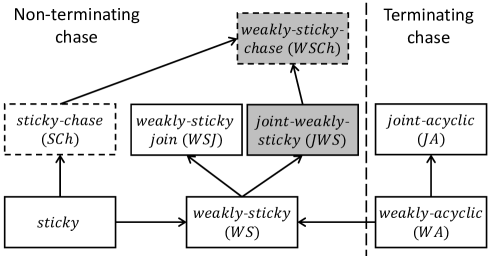
Figure 13: Generalization relationships between program classes. Those depicted with dotted lines are semantic. Those highlighted in grey have been introduced in this work.

Several research directions are part of our ongoing and future work. Among them we find the following:

1. The investigation of the application the magic-set rewriting for Datalog^± in the presence of program constraints, i.e. negative constraints and equality generating dependencies.

2. The implementation of ${\sf SChQA}^{\mathcal{S}}$ and MagicD⁺  and experiments on large real-world data.

   We find particularly interesting in this direction trying out an in-database approach, that is, the implementation of our QA algorithm inside the database, as opposed to having it as an application program running in interaction with the database.

3. We want to study the application of QA ideas in this paper (semantic generalization of program classes, freezing nulls and chase resumption) for QA over programs in different classes of Datalog^± programs.

4. The problem of representing and reasoning about Datalog with numerical and set aggregates has received considerable interest [14, 15, 41, 43]. We intend to study the ${\sf SChQA}^{\mathcal{S}}$ algorithm for Datalog^± with aggregation. Numerical aggregations have been recently introduced for Warded Datalog, a different class of Datalog^± programs [15].

5. As mentioned in Section 1, the motivation for our work had origin in applications of Datalog^± to problems of quality data extraction [13]. Now, we would like to investigate the application of the QA algorithm and its optimization in that scenario.

Acknowledgements:  This work was supported by NSERC Discovery Grants 2016-06148 and 2021-04120, the NSERC Strategic Network on Business Intelligence (BIN), and by ANID - Millennium Science Initiative Program - Code ICN17002.

References

- Abiteboul et al. [1995] Abiteboul, S., Hull, R. and Vianu, V. Foundations of Databases. Addison-Wesley, 1995.
- Alviano et al. [2012] Alviano, M., Faber, W., Leone, N. and Manna, M. Disjunctive Datalog with Existential Quantifiers: Semantics, Decidability, and Complexity Issues. Theory and Practice of Logic Programming (TPLP), 2012, 12(4-5): 701-718.
- Alviano et al. [2012] Alviano, M., Leone, N., Manna, M., Terracina, G. and Veltri, P. Magic-Sets for Datalog with Existential Quantifiers. In Proc. of the International Conference on Datalog in Academia and Industry 2.0, 2012, Springer LNCS 7494, pp. 31-43, DOI: 10.1007/978-3-642-32925-8_5.
- Arenas et al. [2014] Arenas, M., Gottlob, G. and Pieris, A. Expressive Languages for Querying the Semantic Web. In Proc. of the ACM SIGMOD-SIGACT Symposium on Principles of Database Systems (PODS), 2014, pp. 14-26.
- [5] Artale, A., Calvanese, D., Kontchakov, R. and Zakharyaschev, M. The DL-Lite Family and Relations. Journal of Artificial Intelligence, 36, 2009, pp. 1-69.
- Baget et al. [2009] Baget, J. F., Leclére, M., Mugnier, M. L. and Salvat, E. Extending Decidable Cases for Rules with Existential Variables. In Proc. of the International Joint Conference on Artificial Intelligence (IJCAI), 2009, pp. 677-682.
- Baget et al. [2011a] Baget, J. F., Mugnier, M. L., Rulolph, S. and Thomazo, M. Walking the Complexity Lines for Generalized Guarded Existential Rules. In Proc. of the International Joint Conference on Artificial Intelligence (IJCAI), 2011, pp. 712-717.
- Baget et al. [2011b] Baget, J. F., Leclére, M., Mugnier, M.L. and Salvat, E. On Rules with Existential Variables: Walking the Decidability Line. Artificial Intelligence, 2011, 175(9-10): 1620-1654.
- Barcelo [2009] Barcelo, P. Logical Foundations of Relational Data Exchange. ACM SIGMOD Record, 2009, 38(1):49-58.
- Beeri & Vardi [1981] Beeri, C. and Vardi, M. Y. The Implication Problem for Data Dependencies. In Proc. of the Colloquium on Automata, Languages and Programming (ICALP), 1981, Springer LNCS 115, pp. 73-85.
- Beeri & Ramakrishnan [1987] Beeri, C. and Ramakrishnan, R. On the Power of Magic. In Proc. of the ACM SIGMOD-SIGACT Symposium on Principles of Database Systems (PODS), 1987, pp. 269-284.
- Bellomarini et al. [2018] Bellomarini, L., Sallinger, E. and Gottlob G. The Vadalog System:Datalog-based Reasoning for Knowledge Graphs. In Proc. of the International Conference on Very Large Data Bases (VLDB), 2018, pp. 975-987.
- Bertossi & Milani [2017] Bertossi, L. and Milani, M. Ontological Multidimensional Data Models and Contextual Data Quality. Journal of Data and Information Quality (JDIQ). 2018, 9(3): Article 14.
- Bertossi et. al [2018] Bertossi, Leopoldo and Gottlob, G., and Pichler, R. Datalog: Bag semantics via set semantics. Proc. of the International Conference on Database Theory (ICDT), 2019, pp. 16:1-16:19.
- Bellomarini et. al [2018] Bellomarini, L., Sallinger, E., and Gottlob, G. The Vadalog System: Datalog-Based Reasoning for Knowledge Graphs. VLDB Endowment, 2018, 9(11):975–987.
- Calì et al. [2009] Calì, A., Gottlob, G. and Lukasiewicz, T. Datalog±: A Unified Approach to Ontologies and Integrity Constraints. In Proc. of the International Conference on Database Theory (ICDT), 2009, pp. 14-30.
- Calì et al. [2010a] Calì, A., Gottlob, G. and Pieris, A. Advanced Processing for Ontological Queries. In Proc. VLDB Endowment (PVLDB), 2010, 3(1-2): 554-565.
- Calì et al. [2010b] Calì, A., Gottlob, G., Lukasiewicz, T., Marnette, B. and Pieris, A. Datalog±: A Family of Logical Knowledge Representation and Query Languages for New Applications. In Proc. of the Annual IEEE Symposium on Logic in Computer Science (LICS), 2010, pp. 228-242.
- Calì et al. [2011] Calì, A., Gottlob, G., Lukasiewicz, T. and Pieris, A. A Logical Toolbox for Ontological Reasoning. ACM SIGMOD Record, 2011, 40(3): 5-14.
- Calì et al. [2012a] Calì, A., Gottlob, G. and Pieris, A. Ontological Query Answering under Expressive Entity-Relationship Schemata. Information Systems, 2012, 37(4): 320-335.
- Calì et al. [2012b] Calì, A., Gottlob, G. and Lukasiewicz, T. A General Datalog-Based Framework for Tractable Query Answering over Ontologies. Web Semantics, 2012, 14:57-83.
- Calì et al. [2012c] Calì, A., Gottlob, G. and Pieris, A. Towards More Expressive Ontology Languages: The Query Answering Problem. Artificial Intelligence, 2012, 193:87-128.
- Calì et al. [2013] Calì, A., Gottlob, G. and Kifer, M. Taming the Infinite Chase: Query Answering under Expressive Relational Constraints. J. of Artificial Intelligence Research (JAIR), 2013, 48(1): 115-174.
- Calvanese et al. [2007] Calvanese, D., Giacomo, G.C., Lembo, D., Lenzerini, M. and Rosati, R. Tractable Reasoning and Efficient Query Answering in Description Logics: The DL-Lite Family. J. of Automated Reasoning, 2007, 39(3): 385-429.
- Ceri et al. [1990] Ceri, S., Gottlob, G. and Tanca, L. Logic Programming and Databases. Springer, 1990.
- Deutsch et al. [2008] Deutsch, A., Nash, A. and Remmel, J. The Chase Revisited. In Proc. of the ACM SIGMOD-SIGACT Symposium on Principles of Database Systems (PODS), 2008, pp. 149-158.
- Fagin et al. [2005] Fagin, R., Kolaitis, P. G., Miller, R. J. and Popa, L. Data Exchange: Semantics and Query Answering. Theoretical Computer Science (TCS), 2005, 336(1): 89-124.
- Gottlob et al. [2014] Gottlob, G., Orsi, G. and Pieris, A. Query Rewriting and Optimization for Ontological Databases. ACM Trans. Database Syst., 2014, 39(3): 25:1-25:46.
- Johnson & Klug [1984] Johnson, D. S. and Klug, A. Testing Containment of Conjunctive Queries under Functional and Inclusion Dependencies. In Proc. of the ACM SIGMOD-SIGACT Symposium on Principles of Database Systems (PODS), 1984, pp. 164-169.
- Kolaitis et al. [2006] Kolaitis, P. G., Tan, W. C. and Panttaja, J. The Complexity of Data Exchange. In Proc. of the ACM SIGMOD-SIGACT Symposium on Principles of Database Systems (PODS), 2006, pp. 30-39.
- Krötzsch & Rudolph [2011a] Krötzsch, M. and Rudolph, S. Extending Decidable Existential Rules by Joining Acyclicity and Guardedness. In Proc. of the International Joint Conference on Artificial Intelligence (IJCAI), 2011, pp. 963-968.
- Krötzsch & Rudolph [2011b] Krötzsch, M. and Rudolph, S. Revisiting Acyclicity and Guardedness Criteria for Decidability of Existential Rules. Technical Report 3011, Institute AIFB, KIT.
- Leone et al. [2012] Leone, N., Manna, M., Terracina, G. and Veltri, P. Efficiently Computable Datalog∃ Programs. In Proc. of the International Conference on Principles of Knowledge Represenattion and Reasongin (KR), 2012, pp. 13-23.
- Maier et al. [1979] Maier, D., Mendelzon, A. and Sagiv, Y. Testing Implications of Data Dependencies. ACM Transactions on Database Systems (TODS), 1979, 4(4): 455-469.
- Meier et al. [2009] Meier, M., Schmidt, M. and Lausen, G. On Chase Termination Beyond Stratification. In Proc. VLDB Endowment (PVLDB), 2009, 2(1): 970-981.
- Meier et al. [2009] Meier, M., Schmidt, M. and Lausen, G. On Chase Termination Beyond Stratification, Technical Report. Corr ArXiv paper abs/0906.4228, 2009.
- Marnette [2009] Marnette, B. Generalized Schema-Mappings: from Termination to Tractability. In Proc. of the ACM SIGMOD-SIGACT Symposium on Principles of Database Systems (PODS), 2009, pp. 13-22.
- Milani & Bertossi [2015a] Milani, M. and Bertossi, L. Tractable Query Answering and Optimization for Extensions of Weakly-Sticky Datalog. In Proc. of the Alberto Mendelzon International Workshop on Foundations of Data Management (AMW), CEUR-WS Proc. Vol. 1378, 2015, pp. 101-105.
- Milani & Bertossi [2015] Milani, M. and Bertossi, L. Ontology-Based Multidimensional Contexts with Applications to Quality Data Specification and Extraction. In Proc. of the International Symposium on Rules and Rule Markup Languages for the Semantic Web (RuleML), Springer LNCS 9202, 2015, pp. 277-293.
- Milani & Bertossi [2016b] Milani, M. and Bertossi, L. Extending Weakly-Sticky Datalog±: Query-Answering Tractability and Optimizations. In Proc. of the International Conference on Web Reasoning and Rule Systems (RR), Springer LNCS 9898, 2016, pp. 128-143.
- Mohapatra and Genesereth [2008] Mohapatra, A., and Genesereth, M. Aggregation in Datalog under set semantics. Technical Report, http://logic.stanford.edu/reports/LG-2012-01.pdf, 2012.
- Poggi et al. [2008] Poggi, A., Lembo, D., Calvanese, D., De Giacomo, G., Lenzerini, M. and Rosati, R. Linking Data to Ontologies. Data Semantics, 2008, 10(1): 133-173.
- Zaniolo et al. [2017] Zaniolo, C., Yang, M., Das, A., Shkapsky, A., Condie, T., Interlandi, and M., Fixpoint Semantics and Optimization of Recursive Datalog Programs with Aggregates. Theory and Practice of Logic Programming (TPLP), 2017, 17(5): 1048-1065.