Particle motion in circularly polarized vacuum pp waves

Abstract

Bialynicki-Birula and Charzynski argued that a gravitational wave emitted during the merger of a black hole binary may be approximated by a circularly polarized wave which may in turn trap particles [1]. In this paper we consider particle motion in a class of gravitational waves which includes, besides circularly polarized periodic waves (CPP) [2], also the one proposed by Lukash [3] to study anisotropic cosmological models. Both waves have a 7-parameter conformal symmetry which contains, in addition to the generic 5-parameter (broken) Carroll group, also a 6th isometry. The Lukash spacetime can be transformed by a conformal rescaling of time to a perturbed CPP problem. Bounded geodesics, found both analytically and numerically, arise when the Lukash wave is of Bianchi type VI. Their symmetries can also be derived from the Lukash-CPP relation. Particle trapping is discussed.

I Introduction

Bialynicki-Birula and Charzynski (BBC) BB argued that the gravitational waves emitted during the merger of compact binaries may trap massive particles. Their clue is that in the vicinity of the wave axis a gravitational wave carrying angular momentum can be approximated by a Bessel beam. Then for small deviations the geodesic deviation equations yield a coupled system, their eqn. # (14), which admits bounded solutions shown in their fig. 1 – just like their electromagnetic counterparts do BB04 ; Ilderton ; BBBNew .

Their result is consistent with what was found before for Circularly Polarized Periodic (CPP) gravitational waves exactsol , whose geodesic equation can be reduced to similar equations POLPER ; IonGW . Our paper extends and amplifies these findings by studying, both analytically and numerically, geodesic motion in Lukash plane gravitational waves considered before in the study of the isotropy/anisotropy of cosmological models LukashJETP75 ; exactsol ; Ehlers .

Gravitational plane waves have a generic 5-parameter isometry group Sou73 ; BoPiRo ; exactsol , identified as a “broken Carroll” group LL ; Carroll4GW . CPP and Lukash waves are special in that they have an additional 6th “screw” (or “helical” CKlein ) isometry exactsol ; POLPER ; Ilderton . The isometry group extends to a 7-parameter conformal symmetry Ehlers ; Conf4pp ; Conf4GW .

The 6th isometry, which is a sort of “spiralling time translation”, arises for our circularly polarized waves. Moreover, according to Table 24.2 of exactsol p.385, CPP and Lukash are the only vacuum pp waves with this property.

The properties of CPP waves are widely known exactsol ; Ehlers ; our principal interest here is to study the analogous but less-known Lukash waves. Our clue is to reduce the geodesic motion in a Lukash metric to one in a perturbed CPP wave by a clever rescaling ot time, (II.13) below. Exact analytic solutions can be found by following a “road map” outlined in sec. II.2. The solvability comes from transforming the system to one with constant coefficients, (II.16) – which implies also the extra 6th symmetry. Bounded motions arise when the Lukash metric has Bianchi type VI .

Our strategy fits into the framework proposed by Gibbons GWG_Schwarzian . A bonus obtained from our CPP $\leftrightarrow$ Lukash correspondence is to relate their 6th isometries, see sec.IV.

The subtle notion of particle trapping is discussed in sec.V.

Before starting our study we fix our conventions. Lower-case latin letters as ${\bf x}=(x^{1},x^{2}),u,v$ refer to generic pp waves. Latin capitals ${\bf X}=(X^{1},X^{2}),\,U,V,\,Z=\frac{X^{1}+iX^{2}}{\sqrt{2}}$ refer to Lukash waves with profile functions ${{\mathcal{A}_{+}}}(U)$ and ${\mathcal{A}_{\times}}(U)$, respectively; greek letters $\bm{\xi}=(\xi,\eta),\,\zeta=\frac{\xi+i\eta}{\sqrt{2}}$, completed with $T$ and $\nu$ and profile ${\mathcal{B}_{+}}(T)$ and $\mathcal{B}_{\times}(T)$ refer to CPP(-type) waves.

II Circularly polarized gravitational waves 

Both CPP and Lukash waves are plane gravitational waves described, in Brinkmann coordinates, in terms of a symmetric and traceless $2\times 2$ matrix $K_{ij}(u)$ exactsol ; LukashJETP75 ; Ehlers ; Lukash-I ,

$$ds^{2}=d{\bf x}^{2}+2dudv+K_{ij}(u)x^{i}x^{j}du^{2}\,,$$ (II.1)

where ${\bf x}=\big{(}x^{1},x^{2}\big{)}$. The vacuum Einstein equations reduce to $\bigtriangleup\big{(}K_{ij}(u){x^{i}}{x^{j}}\big{)}=0$, where $\bigtriangleup\equiv\bigtriangleup_{2}$ is the transverse-space Laplacian. (II.1)-(II.2) is therefore an exact plane wave for any profile $K_{ij}(u)$.

The profile is decomposed into $+$ and $\times$ polarization states,

$$K_{ij}(u){x^{i}}{x^{j}}=\hbox{$\textstyle\frac{1}{2}$}{{\mathcal{A}_{+}}}(u)\big{(}(x^{1})^{2}-(x^{2})^{2}\big{)}\,+\,\mathcal{A}_{\times}(u)\,x^{1}x^{2}\,.$$ (II.2)

A spin-zero particle moves along a geodesic, described by,

$${\bf x}^{\prime\prime}-K(u)\,{\bf x}=0\quad{\quad\text{where}\quad}\quad K(u)=\hbox{$\textstyle\frac{1}{2}$}\left(\begin{array}[]{lr}{{\mathcal{A}_{+}}}&{\mathcal{A}_{\times}}\\ {\mathcal{A}_{\times}}&-{{\mathcal{A}_{+}}}\end{array}\right),$$ (II.3c)

$$v^{\prime\prime}+{{\mathcal{A}_{+}}}^{\prime}\left((x^{1})^{2}-(x^{2})^{2}\right)+{{\mathcal{A}_{+}}}\left(x^{1}{(x^{1})}^{\prime}-x^{2}{(x^{2})}^{\prime}\right)+{\mathcal{A}_{\times}}^{\prime}x^{1}x^{2}+{\mathcal{A}_{\times}}\left(x^{2}{(x^{1})}^{\prime}+x^{1}{(x^{2})}^{\prime}\right)=0\,,$$ (II.3d)

where the prime means derivative w.r.t. the affine parameter $u$, $\{\,\cdot\,\}^{\prime}=d/du$ .

For any affine parameter $\sigma$ the quantity $-g_{\mu\nu}\dot{x}^{\mu}\dot{x}^{\mu}=m^{2}$ where the “dot” means $d/d\sigma$ is a constant of the motion, identified with the relativistic mass-square. The transverse motion described by (II.3c) does not depend on $m$, and the solution of the $V$-equation differs from that for $m=0$ by the simple shift $m^{2}u$ EDAHKZ , allowing us to restrict our attention at massless geodesics. After solving the transverse equations (II.3c) the $v$-equation is solved by,

$$v(u)=v_{0}-S(u)\,,$$ (II.4)

where $S(u)$ is the Hamiltonian action calculated along the transverse trajectory Bargmann ; dgh91 ; EDAHKZ . Therefore it is enough to solve the transverse equations (II.3c).

In what follows, we restrict our attention at circularly polarized waves. A CPP wave has, for example, the profile (with a slight change of notations ${\cal A}\to{\cal B}$ and $u\to T$).

$${\mathcal{B}_{+}}(T)=-C\,\cos\big{(}\omega T\big{)},\qquad\mathcal{B}_{\times}(T)=C\,\sin\big{(}\omega T\big{)}\,,{\quad\text{where}\quad}C\,,\omega=\mathop{\rm const.}\nolimits$$ (II.5)

The geodesic motion in a CPP can be determined both numerically and analytically POLPER ; IonGW .

II.1 Lukash Geodesics

A Lukash plane gravitational wave is described, in complex form SiklosAll , by

$$ds^{2}_{L}=2dUdV+2dZd\bar{Z}-2C\mathrm{Re}[U^{2(i\kappa-1)}Z^{2}]dU^{2}\,,{\quad\text{where}\quad}Z=\frac{X^{1}+iX^{2}}{\sqrt{2}}\,.$$ (II.6)

The coordinates are well-defined for either $U>0$ or $U<0$ but break down at $U=0$. The nature of the singularity at $U=0$ was the subject of intensive investigations Collins ; LukashJETP75 ; SiklosAll . The constant $C$ determines the strength of the wave; $C\geq 0$ can be chosen with no loss of generality. $\kappa$ is the frequency (inverse wavelength) ; its sign is the (right or left) polarisation. In what follows we shall choose $\kappa>0$. Then for an arbitrary affine parameter $\sigma$ we have the null-geodesic equations,

$$\frac{d^{2}Z}{d\sigma^{2}} \;+\;CU^{-2(i\kappa+1)}\bar{Z}=0\,,$$ (II.7a)

$$\frac{d^{2}V}{d\sigma^{2}} \;-\;2C\left\{\frac{\;\;d}{d\sigma}\mathrm{Re}\big{[}U^{2(i\kappa-1)}Z^{2}\big{]}\frac{dU}{d\sigma}-\mathrm{Re}\big{[}(i\kappa-1)U^{2(i\kappa-1)}Z^{2}U^{-2(i\kappa+1)}\bar{Z}^{2}\big{]}\big{(}\frac{dU}{d\sigma}\big{)}^{2}U^{-1}\right\}=0\,.$$ (II.7b)

${d^{2}U}/{d\sigma^{2}}=0$, implying that $U$ is an affine parameter itself. Reversing the sign of the light-cone coordinates,

$$U\to-U,\qquad V\to-V\,,$$ (II.8)

leaves the Lukash metric (II.6), and consequently also the equations (II.7) invariant. Choosing $U>0$ henceforth, we can switch to more familiar real coordinates, in terms of which the Lukash (II.6) is,

$$ds^{2}_{L} = d{\bf X}^{2}+2dUdV$$ (II.9)

$$-\left\{\frac{C}{U^{2}}\cos\Big{(}2\kappa\ln(U)\Big{)}\,\big{[}(X^{1})^{2}-(X^{2}]^{2}\big{)}\,-\,\frac{2C}{U^{2}}\sin\Big{(}2\kappa\ln(U)\Big{)}\,X^{1}X^{2}\right\}\,dU^{2}\,.$$

The transverse equations form a complicated coupled Sturm-Liouville system,

$$\left(\begin{array}[]{cc}(X^{1})^{\prime\prime}\\[3.0pt] (X^{2})^{\prime\prime}\end{array}\right)=-\frac{C}{U^{2}}\left(\begin{array}[]{rr}\cos(2\kappa\ln U)&-\sin(2\kappa\ln U)\\[3.0pt] -\sin(2\kappa\ln U)&-\cos(2\kappa\ln U)\end{array}\right)\left(\begin{array}[]{cc}X^{1}\\[3.0pt] X^{2}\end{array}\right)\,$$ (II.10)

where now $\{\,\cdot\,\}^{\prime}=d/dU$ .

Let us recall, for the sake of comparison, “ordinary” CPP : the transverse equations of motion of the metric (II.1) with profile (II.5) are

$$\left(\begin{array}[]{cc}\ddot{\xi}\\[2.0pt] \ddot{\eta}\end{array}\right)=-{C}\left(\begin{array}[]{rr}\cos\omega T&+\sin\omega T\\[2.0pt] \sin\omega T&-\cos\omega T\end{array}\right)\left(\begin{array}[]{cc}\xi\\[2.0pt] \eta\end{array}\right)\,$$ (II.11)

where $\omega=\mathop{\rm const.}\nolimits$ (We changed notation, $x^{1}\to\xi,\,x^{2}\to\eta,u\to T,\,\dot{\{\,\cdot\,\}}=d/dT$ on purpose). Having chosen $C>0$, bounded solutions arise when

$$\big{(}\frac{\omega}{2}\big{)}^{2}-C>0\,.$$ (II.12)

Lukash and CPP are thus similar but still different.

II.2 Solution of the Sturm-Liouville equations

Sturm-Liouville equations are notoriously difficult to solve. Analytic solutions can be found in our case, though, by the following steps.

$\bullet$ Our clue is to switch to “logarithmic time” and introduce new transverse coordinates,

$$\;\;\displaystyle{U=e^{T}\,,\quad{\bf X}=e^{T/2}\bm{\xi},{\quad\text{where}\quad}\bm{\xi}={\tiny\left(\begin{array}[]{c}\xi\\ \eta\end{array}\right)},}\;\;$$ (II.13)

in terms of which (II.10) becomes,

$$\;\;\displaystyle{\frac{\;\;d^{2}}{dT^{2}}\left(\begin{array}[]{c}\xi\\ \eta\end{array}\right)=\text{linear}+\text{CPP}=\frac{1}{4}\left(\begin{array}[]{c}\xi\\ \eta\end{array}\right)-C\left(\begin{array}[]{rr}\cos(2\kappa T)&-\sin(2\kappa T)\\ -\sin(2\kappa T)&-\cos(2\kappa T)\end{array}\right)\left(\begin{array}[]{c}\xi\\[3.0pt] \eta\end{array}\right)\,.}\;\;$$ (II.14)

Comparison with (II.11) shows that the projected non-relativistic dynamics is that of a repulsive linear force with spring constant $\textstyle\frac{1}{4}$, combined with a periodic “CPP” force. The latter may be attractive or repulsive depending on the amplitude $C>0$ and the frequency, $-2\kappa$ exactsol ; POLPER ; IonGW .

$\bullet$ Our second step is to change again to new position coordinates, $\binom{\alpha}{\beta}$. The rotation with half-of-the-angle BB ; POLPER (suggested to us by Piotr Kosinski) ,

$$\binom{\xi}{\eta}=R_{\kappa T}\binom{\alpha}{\beta}\,,\quad R_{\kappa T}=\left(\begin{array}[]{cc}\cos\kappa T&+\sin\kappa T\\ -\sin\kappa T&\;\cos\kappa T\end{array}\right)$$ (II.15)

converts (II.14) into a coupled Coriolis-type system with constant coefficients,

$$\ddot{\alpha}+2\kappa\,\dot{\beta}-\Omega_{-}^{2}\,\alpha=0\,,$$ (II.16a)

$$\ddot{\beta}-2\kappa\,\dot{\alpha}-\Omega_{+}^{2}\,\beta=0\,,$$ (II.16b)

where the dot $\dot{\{\,\cdot\,\}}$ means, henceforth, $d/dT$,

$$\Omega_{-}^{2}=\left(\kappa^{2}+\frac{1}{4}-C\right){\quad\text{and}\quad}\Omega_{+}^{2}=\left(\kappa^{2}+\frac{1}{4}+C\right)\,.$$ (II.17)

Our oscillator is anisotropic, $\Omega_{+}^{2}-\Omega_{-}^{2}=2C$ ; the lower frequency may become negative, depending on the parameters.

Remarkably, the system (II.16) coincides with the equations #(14) of Bialynicki-Birula and Charzynski BB , who obtained it after a series of approximations. In the Eisenhart-Duval framework Bargmann ; dgh91 it would describe a charged anisotropic linear oscillator in the plane with frequencies $\Omega_{\pm}$ , put into a uniform magnetic field $B=-2\kappa$. Its behavior is determined by the subtle competition between the magnetic and oscillating terms, as it will be illustrated by our figures below.

$\bullet$ Our last step comes from that the equations (II.16) are up to the frequency-shift $1/4$ those for a CPP exactsol ; BB ; IonGW and can thus be solved analytically BB ; Plyuchir ; IonGW . We start with the Hamiltonian and symplectic form,

$${\mathcal{H}} =\hbox{$\textstyle\frac{1}{2}$}{\bm{p}}^{2}-\hbox{$\textstyle\frac{1}{2}$}(\Omega_{-}^{2}\alpha^{2}+\Omega_{+}^{2}\beta^{2})\,,$$ (II.18a)

$$\sigma =dp^{i}\wedge d\alpha^{i}-\kappa\,\varepsilon^{ij}d\alpha^{i}\wedge d\alpha^{j}\,$$ (II.18b)

and introduce four phase-space coordinates $\,w_{\pm}^{1},w_{\pm}^{2}$ by setting

$$p^{1} =\mu_{+}w_{+}^{2}+\mu_{-}w_{-}^{2}\,\hskip 56.9055ptp^{2}=-\nu_{+}w_{+}^{1}-\nu_{-}w_{-}^{1}\,,$$ (II.19a)

$$\alpha =w_{+}^{1}\;+\;w_{-}^{1}\,,\hskip 73.97716pt\beta\,=w_{+}^{2}\;+\;w_{-}^{2}\,.$$ (II.19b)

Then choosing the coefficients as,

$$\mu_{+}=\dfrac{1}{2\kappa}\left(\sqrt{C^{2}-\kappa^{2}}-2\kappa^{2}-C\right)\,, \nu_{+}=\;\;\dfrac{1}{2\kappa}\left(\sqrt{C^{2}-\kappa^{2}}-2\kappa^{2}+C\right)\,,\,$$ (II.20a)

$$\mu_{-}=-\dfrac{1}{2\kappa}\left(\sqrt{C^{2}-\kappa^{2}}+2\kappa^{2}+C\right)\,, \quad\,\nu_{-}=-\dfrac{1}{2\kappa}\left(\sqrt{C^{2}-\kappa^{2}}+2\kappa^{2}-C\right)\,,$$ (II.20b)

decomposes the system into two uncoupled 1D Hamiltonian systems with opposite relative signs,

$$\sigma=\sigma_{+}-\sigma_{-}\,,\qquad H=H_{+}-H_{-}\,,$$ (II.21)

where

$$\sigma_{+} =-\dfrac{\sqrt{C^{2}-\kappa^{2}}}{\kappa}\;dw_{+}^{1}\wedge dw_{+}^{2}\,,\qquad H_{+}=\;\;\dfrac{\sqrt{C^{2}-\kappa^{2}}}{2\kappa}\left[\nu_{+}\,w_{+}^{1}w_{+}^{1}+\mu_{+}\,w_{+}^{2}w_{+}^{2}\right]\,,$$ (II.22a)

$$\sigma_{-} =-\dfrac{\sqrt{C^{2}-\kappa^{2}}}{\kappa}\;dw_{-}^{1}\wedge dw_{-}^{2}\,,\qquad H_{-}=\dfrac{\sqrt{C^{2}-\kappa^{2}}}{2\kappa}\left[\nu_{-}\,w_{-}^{1}w_{-}^{1}+\mu_{-}\,\,,w_{-}^{2}w_{-}^{2}\right]\,,$$ (II.22b)

respectively.

Strong but slow perturbation: $C>\kappa$ .

For $C>\kappa$  $\sigma_{\pm}$ and $H_{\pm}$ in (II.22) are real and the Hamiltonian system is regular. The associated equations of motion are

$$\ddot{w}_{+}^{1}+\lambda_{+}^{2}\,w_{+}^{1}=0\,,\qquad\ddot{w}_{+}^{2}+\lambda_{+}^{2}\,w_{+}^{2}=0\,,$$ (II.23a)

$$\ddot{w}_{-}^{1}+\lambda_{-}^{2}\,w_{-}^{1}=0\,,\qquad\ddot{w}_{-}^{2}+\lambda_{-}^{2}\,w_{-}^{2}=0\,,$$ (II.23b)

where the two effective frequency-squares are,

$$\lambda_{+}^{2}=\mu_{+}\,\nu_{+}=\kappa^{2}-\hbox{$\textstyle\frac{1}{4}$}-\sqrt{C^{2}-\kappa^{2}}\quad{\quad\text{and}\quad}\quad\lambda_{-}^{2}=\mu_{-}\,\nu_{-}=\kappa^{2}-\hbox{$\textstyle\frac{1}{4}$}+\sqrt{C^{2}-\kappa^{2}}\,.$$ (II.24)

The equations (II.23) are not independent, though: $w_{+}$ and $w_{-}$ have to satisfy $\dot{w}^{1}_{+}=\mu_{+}w^{2}_{+}$ and $\dot{w}^{1}_{-}=\mu_{-}w^{2}_{-}\,,$ which eliminates half of the integration constants and we end up with two independent oscillations with frequencies $\lambda_{\pm}$,

$$w_{+}^{1} =a\cos\lambda_{+}T+b\sin\lambda_{+}T,~{}~{}~{}~{}~{}w_{+}^{2}=\;\sqrt{\frac{\nu_{+}}{\mu_{+}}}\left(-a\sin\lambda_{+}T+b\cos\lambda_{+}T\right)\,,$$ (II.25a)

$$w_{-}^{1} =c\cos\lambda_{-}T+d\sin\lambda_{-}T,~{}~{}~{}~{}~{}w_{-}^{2}=-\sqrt{\frac{\nu_{-}}{\mu_{-}}}\left(c\sin\lambda_{-}T-d\cos\lambda_{-}T\right)\,,$$ (II.25b)

where $a,b,c,d$ are free real constants. These equations show that bounded solutions arise when both lambdas are real, as illustrated below in figs.2,3 and 5. In view of (II.19b) the chiral decomposition can be interpreted as follows: in the rotating frame the transverse-space trajectory is decomposed into a sum,

$$\left(\begin{array}[]{c}\alpha(T)\\ \beta(T)\end{array}\right)=\left(\begin{array}[]{c}w_{+}^{1}(T)\\ w_{+}^{2}(T)\end{array}\right)+\left(\begin{array}[]{c}w_{-}^{1}(T)\\ w_{-}^{2}(T)\end{array}\right)\,,$$ (II.26)

where the first term represents a sort of “guiding center” and the second describes a sort of “epicycle” around it. Proceeding backwards, from (II.15) we infer $\binom{\xi}{\eta}=R_{(\kappa T)}\binom{\alpha}{\beta}$ and then ${\bf X}(U)$ can be deduced from (II.13). Bounded $\binom{\alpha}{\beta}$ [or $\binom{\xi}{\eta}$] motions arise when both frequency-squares are positive, which happens when $\lambda_{\pm}^{2}>0$ that requires

$$\;\;\displaystyle{\kappa<C<C_{crit}=\kappa^{2}+\hbox{$\textstyle\frac{1}{4}$}{\quad\text{with}\quad}\kappa>1/2,\,}\;\;$$ (II.27)

studied before by Siklos SiklosAll and illustrated in fig.1 below, strongly reminiscent of fig.1 in BB . See also PaulRMP ; Kirillov . Expressed in Brinkmann terms

$${\bf X}(U)=\sqrt{U}\,R_{(\kappa\ln U)}\binom{\alpha}{\beta}$$ (II.28)

and therefore the trajectories escape. Boundedness/unboudness will be further discussed in sec.V.

The metric admits a 3-parameter group of motions acting on spacelike hypersurfaces if and only if either $\kappa\leq\hbox{$\textstyle\frac{1}{2}$}$ and $0\leq C\leq\kappa^{2}+\hbox{$\textstyle\frac{1}{4}$}\,,$ or $\kappa\geq\hbox{$\textstyle\frac{1}{2}$}$ and $0\leq C\leq\kappa\,$ SiklosAll . The group type (with some overlaps) is :

• Bianchi VII: if

  $$\text{either}\quad 0\leq C<\kappa\quad\text{or}\quad C=\kappa>\hbox{$\textstyle\frac{1}{2}$}$$ (II.29)

• Bianchi VI: if

  $$\text{either}\quad\kappa<C\leq\kappa^{2}+\hbox{$\textstyle\frac{1}{4}$}\quad\text{or}\quad 0<C=\kappa<\hbox{$\textstyle\frac{1}{2}$}$$ (II.30)

• Bianchi IV: if

  $$C=\kappa$$ (II.31)

It follows that bound motion arise only when the wave is of Bianchi-VI type.

Below we study the behavior for various values of the parameters.

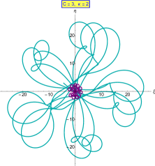
Figure 1: In terms of logarithmic position coordinates $\binom{\xi}{\eta}$ (II.13) (or their rotated versions $\binom{\alpha}{\beta}$ (II.15)) one gets bounded Lukash trajectories in the parameter range (II.27). The magenta curve near the origin is the contribution of the “CPP” term in (II.14), which is pushed outwards by the repulsive force. However the CPP term keeps the motion bounded.

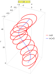
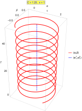
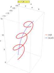
(a)                                   (b)                                    (c)

Figure 2: Trajectories shown in $\binom{\alpha}{\beta}$ coordinates unfolded in logarithmic time $T$ when close to the upper critical value $C_{crit}$. The motion of the guiding center ${{\bf w}}_{+}$ is determined by $\lambda_{+}^{2}$ and the “epicycle” around it is described by ${\bf w}_{-}$, determined by ${\color[rgb]{1,0,0}\lambda_{-}^{2}}=\lambda_{+}^{2}+2\sqrt{C^{2}-\kappa^{2}}$. (a) when $\kappa<C<C_{crit}=\kappa^{2}+\hbox{$\textstyle\frac{1}{4}$}$ (which has Bianchi type VI), the trajectory remains bounded ; (b) for $C=C_{crit}$ with $\kappa>\hbox{$\textstyle\frac{1}{2}$}$ (which is Bianchi VI), the radius is constant in logarithmic time $T$ (grows linearly in $U$), (c) for $C>C_{crit}$ the trajectory escapes exponentially.

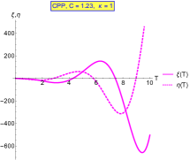
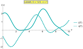
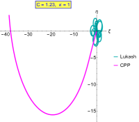
(a)                                                (b)                                                  (c)

Figure 3: Transverse trajectories in $(\xi,\eta)$ coordinates just below the upper critical value $C_{crit}$ for: (a) the CPP term alone, i.e., without the linear perturbation; (b) the full Lukash system. (a) and (b) show the components. Caveat: the CPP and Lukash scales in (a) and (b) repectively are different. (c) shows the transverse trajectories. The motion is bounded for Lukash but unbounded for CPP.

Behaviour at the critical values.

At the upper critical value $C=C_{crit}$ the effective frequencies (II.24) become $\lambda_{+}=0$ and $\lambda_{-}^{2}=2(\kappa^{2}-1/4)$. The motion is unbounded, $w_{+}^{1}=a+b\,T,\,w_{+}^{2}=c+d\,T\,,$ while $w_{-}$ either oscillates or escapes, depending on $\kappa$ being above or below $1/2$. The behavior for $C$ close to $C_{crit}$ is illustrated in figs. 2, 3 5. For $C>C_{crit}$ the motion escapes rapidly .

At the lower limiting value $C=\kappa$ in (II.31) both the symplectic forms and Hamiltonians (II.22) vanish and we have to return to the equations (II.16) with $\Omega_{\mp}^{2}=(\kappa\mp\hbox{$\textstyle\frac{1}{2}$})^{2}$. Then we consider three subcases, illustrated in figs.4 and 5.

• For $0<C=\kappa<\frac{1}{2}\,$ (which is Bianchi VI) we get in the rotating coordinates $\binom{\alpha}{\beta}$ in (II.15),

  $$\alpha= \left(a-\kappa\big{(}\frac{2b+(1+2\kappa)c}{1-2\kappa}\big{)}T\right)\cosh\bar{\omega}T\,+$$

  $$\left(\frac{b+(1+2\kappa)\kappa c}{1-2\kappa}-\frac{\kappa}{2}\big{(}(1-2\kappa)a+2d\big{)}T\right)\frac{\sinh\bar{\omega}T}{\bar{\omega}}\,,$$

  $$\beta= \left(c+\kappa\big{(}\frac{(1-2\kappa)a+2d}{1+2\kappa}\big{)}T\right)\cosh\bar{\omega}T\,+$$ (II.34)

  $$\left(\frac{-(1-2\kappa)\kappa a+d}{1+2\kappa}+\kappa\big{(}b+(1+2\kappa)2c\big{)}T\right)\frac{\sinh\bar{\omega}T}{\bar{\omega}}\,,$$

  where

  $$\bar{\omega}=\sqrt{\hbox{$\textstyle\frac{1}{4}$}-\kappa^{2}}\,.$$ (II.35)

  The trajectory is exponentially escaping: the rotation is too week to keep the motion bounded.

• For $C=\kappa>\frac{1}{2}\,$ (which is Bianchi VII) we get the same formulae up to replacing hyperbolic functions by trigonometric ones,

  $$\cosh\bar{\omega}\to\cos\tilde{\omega}\,,\quad\sinh\bar{\omega}\to\sin\tilde{\omega}\,{\quad\text{where}\quad}\tilde{\omega}=\sqrt{\kappa^{2}-\hbox{$\textstyle\frac{1}{4}$}}\,,$$ (II.36)

  see fig.4. Exponential escape is eliminated, however terms which are linear in $T=\ln U$ may remain.

• In the Bianchi IV case $C=\kappa=\frac{1}{2},$ the trajectories are polynomial functions of $T$,

  $$\alpha=a+bT-\frac{d}{2}T^{2}-\hbox{$\textstyle\frac{(b+c)}{6}$}T^{3},\;\beta=c+dT+\hbox{$\textstyle\frac{(b+c)}{2}$}T^{2}\,,$$ (II.37)

  which remain bounded only in the trivial case $b=c=d=0$.

The value (II.31) separates our present domain of investigations (II.27) from the Bianchi VII_h range

$$0<C<\kappa\,$$ (II.38)

we studied in Lukash-I using a rather different (“Siklos” SiklosAll ) technique. The results are consistent, though. In the range (II.38) the chiral decomposition (II.22) would yield imaginary symplectic forms and Hamiltonians.

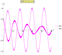
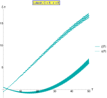
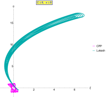
(a)                                                (b)                                            (c)

Figure 4: The components of (a) CPP and (b) Lukash geodesics at the lower critical value $C=\kappa$ (which is Bianchi VII and Bianchi IV). The colors refer to the respective cases. Caveat: the CPP and Lukash scales in (a) and (b) are different. Fig.(c) shows both trajectories in the transverse plane.

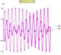
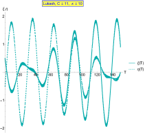
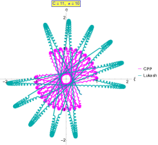
(a)                                            (b)                                            (c)

Figure 5: (a) CPP and (b) Lukash trajectories just above the lower critical value $C=\kappa$. The colors and labels refer to the respective cases. Caveat: the CPP and Lukash scales are different. (c) combines the two curves.

III Lift to 4D

Further insight is provided by lifting the coordinate transformation to 4D Lukash spacetime. Completing (II.13) with $V\to V$ allows us to write the Lukash metric as

$$ds_{L}^{2}=e^{T}d\Sigma^{2}\,,$$ (III.1)

which is conformal to

$$d\Sigma^{2}=d\xi^{2}+d\eta^{2}+2dTdV+({\xi}d\xi+{\eta}d\eta)dT+\big{(}\frac{1}{4}\left(\xi^{2}+\eta^{2}\right)-C\left(\xi^{2}-\eta^{2}\right)\cos 2\kappa T+2C\xi\eta\sin 2\kappa T\big{)}dT^{2}\,.$$ (III.2)

From the Barmann point of view, the geodesics of this metric project to motion in a uniform magnetic field combined with an anisotropic oscillator. The term $({\xi}d\xi+{\eta}d\eta)dT$ can actually be absorbed by a redefinition of the vertical coordinate,

$$V=\nu-\hbox{$\textstyle\frac{1}{4}$}\big{(}\xi^{2}+\eta^{2}\big{)}\,,$$ (III.3)

allowing us to present (III.2) as,

$$d\Sigma^{2}=d\bm{\xi}^{2}+2dTd\nu+\big{(}\frac{1}{4}\bm{\xi}^{2}-C\left(\xi^{2}-\eta^{2}\right)\cos 2\kappa T+2C\xi\eta\sin 2\kappa T\big{)}dT^{2}\,,$$ (III.4)

which differs from the CPP metric only in an additional $\frac{1}{4}\bm{\xi}^{2}$ perturbation of the potential (where we wrote obviously $\bm{\xi}=(\xi,\eta)$). In conclusion,

$$({\bf X},U,V)\to(\bm{\xi},T,\nu)\,,$$ (III.5)

is a conformal mapping from Brinkmann to coordinates with logarithmic time, $T=\ln U$. We shall call it “perturbed CPP metric” in what follows. The latter is not a vacuum solution due to the additional $\bm{\xi}^{2}$ in the potential.

Conformally related metrics have identical null geodesics (and intertwined respective affine parameters) Wald ; the identity of the null geodesics of $ds_{L}^{2}$ and $d\Sigma^{2}$, respectively, can be checked directly.

Henceforce we work with $d\Sigma^{2}$ and we choose $T$ as affine parameter.

We record for later use that applying again the rotational trick (II.15) and putting $A_{\alpha}=\kappa\beta,\,A_{\beta}=-\kappa\alpha\,$ allows us to rewrite $d\Sigma^{2}$ as

$$d\Sigma^{2}=d\alpha^{2}+d\beta^{2}+2\Big{(}d\nu+A_{\alpha}d\alpha+A_{\beta}d\beta\Big{)}dT+\Big{(}\Omega_{-}^{2}\alpha^{2}+\Omega_{+}^{2}\beta^{2}\Big{)}\,dT^{2}\,.$$ (III.6)

$\hbox{$\textstyle\frac{1}{2}$}(\alpha d\alpha+\beta d\beta)=d\left(\hbox{$\textstyle\frac{1}{4}$}\big{(}\xi^{2}+\eta^{2}\big{)}\right)$ is a vector potential for a constant magnetic field $B=-2\kappa$ which can be removed by redefining the vertical coordinate, cf. (III.3).

IV Isometries and conformal transformations

Now we show that the Lukash metric carries a 6-parameter group of isometries which extends to a 7 parameter conformal group. We follow first our road map set out in sec.II.2.

1. The Lukash metric admits the generic 5-parameter broken Carroll symmetry of gravitational plane waves exactsol ; LL ; Carroll4GW ; Torre ; SLC ; Conf4GW spanned by the covariantly constant vector ${\partial}_{V}$ plus of $4$ “U-dependent translations” GiPo ,

   $$X^{1}\to X^{1}+\beta^{1}(U),\qquad X^{2}\to X^{2}+\beta^{2}(U)\,$$ (IV.1)

   that carry solutions into solutions. Then by the linearity of (II.3c) the $\beta^{i}$ have to satisfy the same equations as the transverse coordinates do. Thus the time-dependent symmetries of (II.3c) are the projections of geodesics Carroll4GW . They lift to 4D to isometries by (II.4) and are analogous to what one obtains for an isotropic oscillator by pulling back the translations and boosts of a free particle by Niederer’s map Niederer73 . They span a Newton-Hooke group structure GiPo ; Zhang:2011bm .

2. The remarkable property of the Lukash system is its additional 6th isometry exactsol ; Lukash-I , recovered as follows : in terms of the new coordinates $T=\ln U$, $\binom{\alpha}{\beta}$ and $\nu$ in (II.15)–(III.3) none of the coefficients in the rotated metric (III.6) [or of the equations of motion (II.16)] depends on $T$; therefore $T$-translations,

   $$T\to T+\tau\,,\qquad\binom{\alpha}{\beta}\to\binom{\alpha}{\beta},\qquad\nu\to\nu\,$$ (IV.2)

   are manifest isometries for any real constant $\tau$. Working backwards, the perturbed CPP equations (II.14) are invariant w.r.t. the “screw” obtained by combining a $T$-translation with a transverse rotation with angle $(-\kappa\tau)$ Carroll4GW ; POLPER ; IonGW ,

   $$T\to T+\tau,\qquad\binom{\xi}{\eta}\to R_{(-\kappa\tau)}\,\binom{\xi}{\eta}\,,\qquad\nu\to\nu\,.$$ (IV.3)

   In Brinkmann terms this isometry is implemented as

   $$U\to e^{\tau}\,U,\qquad{\bf X}\to R_{(-\kappa\tau)}{\bf X},\qquad V\to e^{-\tau}\,V\,$$ (IV.4)

   and is generated by combining an U-V boost with a transverse rotation ,

   $$Y_{\kappa}=(U\partial_{U}-V\partial_{V})-\kappa(X^{1}\partial_{2}-X^{2}\partial_{1})\,$$ (IV.5)

   we propose to call “expanding screw”. For $\kappa=0$ the Lukash profile reduces to $U^{-2}$ and the results in Conf4GW ; Conf4pp are recovered.

3. In addition to isometries, we also have the homotheties,

   $$U\to U,\qquad{\bf X}\to\lambda\,{\bf X},\qquad V\to\lambda^{2}V\qquad(\lambda=\mathop{\rm const.}\nolimits>0),$$ (IV.6)

   which are conformal transformations with conformal factor $\lambda^{2}$ Hsu ; Conf4GW . (IV.6) is generated by,

   $$Y_{h}=X^{i}\frac{\partial}{\partial X^{i}}+2V\frac{\partial}{\partial V}\,.$$ (IV.7)

Now we relate the 6th isometry (IV.5) for Lukash to the “screw”, known before for CPP. The latter combines a $T$-translation with a transverse rotation,

$$Y_{s}=\partial_{T}+\frac{\omega}{2}\epsilon_{ij}\xi^{i}\partial_{j}\,.$$ (IV.8)

We first recall how it goes for CPP. Using again the notations ${\bf x}\to\bm{\xi}=(\xi,\eta)$, $u\to T,\,v\to\nu$, the CPP metric (II.1)-(II.2)-(II.5) is written, in complex notation $\zeta={(\xi+i\eta)}/{\sqrt{2}}$ ,

$$ds^{2}_{CPP}=2d\zeta d\bar{\zeta}+2d\nu dT+A_{0}\mathrm{Re}[e^{-i\omega T}\zeta^{2}]dT^{2}.$$ (IV.9)

Then for any $\tau=\mathop{\rm const.}\nolimits$

$$T\to T+\tau,\quad\zeta\to e^{i\tau\omega/2}\zeta\,,\quad\nu\to\nu$$ (IV.10)

leaves the metric (IV.9) invariant POLPER ; exactsol . Infinitesimally, this is generated by

$$Y_{s}=\partial_{T}+i\frac{\omega}{2}\big{(}\zeta\,{\partial}_{\zeta}-\bar{\zeta}\,{\partial}_{\bar{\zeta}}\big{)}\,,$$ (IV.11)

cf. (IV.8). Thus CPP has a 6-parameter isometry group exactsol ; BoPiRo ; Carroll4GW , extended to 7-parameter conformal symmetry by the homothety

$$Y_{h}=\xi^{i}\frac{\partial}{\partial\xi^{i}}+2\nu\partial_{\nu}\,.$$ (IV.12)

Turning to Lukash waves, we assume $U>0$ and start with the real form (II.9) which is conformal to the “perturbed CPP metric” $d\Sigma^{2}$ in (III.2) [or in (III.4)], $ds_{L}^{2}=e^{T}d\Sigma^{2}$ cf. (III.1). $d\Sigma^{2}$ is readily seen to admit also the “screw” isometry

$$Y_{s}=\partial_{T}-\kappa\epsilon_{ij}\xi^{i}\partial_{j},$$ (IV.13)

cf. (IV.8) with $\omega\to-2\kappa$, as well as the homothety (IV.12). These symmetries have to be pulled back to Lukash, which involves the conformal factor $e^{T}$ see (III.1). However we find

$$L_{Y_{h}}\big{(}e^{T}g_{\mu\nu}(\xi,T,V)\big{)} = 2e^{T}g_{\mu\nu}(\xi,T,V),$$ (IV.14)

$$L_{Y_{s}}\big{(}e^{T}g_{\mu\nu}(\xi,T,V)\big{)} = e^{T}g_{\mu\nu}(\xi,T,V)$$ (IV.15)

which are now both conformal. But combining them as,

$$Y_{\kappa}=Y_{s}-\frac{1}{2}Y_{h}=\partial_{T}-V\partial_{V}-\left(\frac{1}{2}\xi^{j}+\kappa\epsilon_{ij}\xi^{i}\right)\frac{\partial}{\partial\xi^{j}},$$ (IV.16)

the conformal factors compensate, providing us finally with an isometry $Y_{\kappa}$,

$$L_{Y_{\kappa}}\big{(}e^{T}g_{\mu\nu}(\xi,T,V)\big{)}=0.$$ (IV.17)

Then returning to our original Brinkmann coordinates by (II.13), the Lukash isometry (IV.5) and the homothety (IV.7) are recovered,

$$Y_{\kappa} = U\partial_{U}-V\partial_{V}-\kappa\epsilon_{ij}X^{i}\partial_{j},$$ (IV.18)

$$Y_{h} = X^{i}\frac{\partial}{\partial X^{i}}+2V\frac{\partial}{\partial V}\,.$$ (IV.19)

We note for completeness that the “expanding screw” (IV.4)–(IV.5) can also be obtained along the same lines as for the CPP screw (IV.10) : the complex forms (II.6)–(II.7) are manifestly invariant under the “expanding screw” transformation

$$U\to e^{\tau}U,\qquad V\to e^{-\tau}V,\qquad Z\to e^{-i\kappa\tau}Z\,.$$ (IV.20)

V Coordinate dependence of bounded/unbounded property

Now, as we realised while answering a question of our referee, we argue that the very notion of “particle trapping” (which appears in the title of ref. BB , and also in the previous version of our paper) may be coordinate dependent : the motion can appear bounded in one coordinate system and unbounded in another one, as we illustrate it on various examples.

1. Let us first consider the Niederer correspondence between a harmonic oscillator of frequency $\omega=\mathop{\rm const.}\nolimits$ and a free particle Niederer73 ; dgh91 ; Andr18 ; ZZH ; Silagadze . The mapping

   $$T=\frac{\tan\omega t}{\omega},\qquad X=\frac{x}{\cos\omega t}$$ (V.1)

   carries the half oscillator-period $-\frac{\pi}{2\omega}<t<\frac{\pi}{2\omega}$ into a full free motion with $-\infty<T<\infty$, whereas the bounded oscillations become unbounded.

2. A similar behavior is observed also for planetary motion with a time-dependent gravitational constant as suggested by Dirac DiracGt , e.g.,

   $$G(t)=G_{0}\frac{t_{0}}{t}\,.$$ (V.2)

   For $t$ close to $t_{0}$, $t\approx t_{0}(1+\epsilon)$. The Bargmann manifolds with $G=G_{0}=\mathop{\rm const.}\nolimits$ and $G=G(t)$, respectively, are conformally related with conformal factor $\Omega^{2}(t)=({t_{0}}/{t})^{2}$ dgh91 . A circular transverse trajectory $\bm{\zeta}(T)=e^{iT}$ for $G=G_{0}$ becomes

   $$t\to T=-{t_{0}^{2}}/{t},\qquad Z(t)=\frac{t}{t_{0}}\,e^{-i{t_{0}^{2}}/{t}}\approx(1+\epsilon)e^{-it_{0}(1-\epsilon)}.$$ (V.3)

   Thus for $G(t)$ in (V.2) the orbit of planetary spirals outwards, as shown in FIG.6 : $G(t)$ decreases with increasing $t$. The gravitational pull weakens, the particle escapes and its rotation slows down.

   Let us note that the relativistic coordinate transformation (V.3) lifted to Bargmann space transforms the two different underlying non-relativistic systems with $G(t)$ and $G_{0}$ into each other.

   

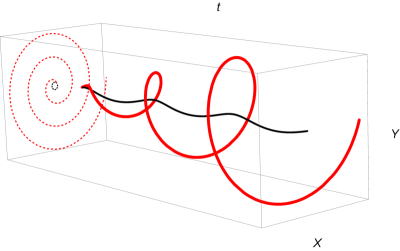
   Figure 6: Planetary motions for gravitational constant ${\bf G_{0}=\mathop{\rm const.}\nolimits}$ and for ${\color[rgb]{1,0,0}\bf G(t)=G_{0}{t_{0}}/{t}}$, respectively, are described by conformally related Bargman manifolds dgh91 . An orbit (in black) which is bounded for $G_{0}$ can become unbounded for ${\color[rgb]{1,0,0}G(t)}$, as illustrated for a circular Newtonian trajectory.

3. Our last example is the motion in the expanding universe as seen by different observers Blau . Since Lukash metric is related with the open Friedmann universe, we consider the flat $(k=0)$ FRW metric

   $$ds^{2}=-dt^{2}+a\left(t\right)^{2}\left(d\rho^{2}+\rho^{2}d\Omega^{2}\right).$$ (V.4)

   With the conformal time

   $$dT=\frac{dt}{a(t)}$$ (V.5)

   the above metric can be expressed using co-moving coordinates $(T,\rho,\theta,\phi)$,

   $$ds^{2}=a(T)^{2}\left(-dT^{2}+d\rho^{2}+\rho^{2}d\Omega^{2}\right)\,.$$ (V.6)

   For the scale factor $a(t)=\sqrt{t}$, for example, one gets the radial trajectory $\theta,\phi=\mathop{\rm const.}\nolimits$,

   $$\rho(T)=\rho_{1}+\frac{\alpha}{2}\ln\left(2T+\sqrt{4T^{2}+\alpha^{2}}\right),\quad\rho_{1}=\mathop{\rm const.}\nolimits$$ (V.7)

   Thus for a co-moving observer staying in the co-moving coordinates $(T,\rho,\theta,\phi)$, the free particle can stay int rest : $\rho(T)=\rho_{1}=\mathop{\rm const.}\nolimits$ when $\alpha=0$.

   Next, we consider global coordinates $\left(t,R,\theta,\phi\right)$, with global time $t$ and position

   $$R\left(t\right)=a\left(t\right)\rho=\sqrt{t}\,\rho\,.$$ (V.8)

   Then the FRW metric (V.6) can be expressed as

   $$ds^{2}=-\left(1-\frac{R^{2}}{4t^{2}}\right)dt^{2}-\frac{R}{t}dR\,dt+dR^{2}+R^{2}d\Omega^{2}$$ (V.9)

   with the radial trajectory becoming

   $$R\left(t\right)=\sqrt{t}\left\{\rho_{1}+\frac{\alpha}{2}\ln\left(4\sqrt{t}+4\sqrt{t+\alpha^{2}/16}\right)\right\}\,.$$ (V.10)

   Thus in the global observer’s coordinates $\left(t,R,\theta,\phi\right)$ the motion of the free particle is unbounded : for a global observer in an expanding universe there is no bounded (localized) motion which, however, may exist for a co-moving observer.

We conclude that the motion being bounded or unbounded may depend on the coordinates we choose.

VI Conclusion

Bialynicki-Birula and his collaborators argue that gravitational waves emitted during the merger of a compact binary system may trap particles BB . Their statement is consistent with our previous study for a CPP wave POLPER ; IonGW for which we had found bounded geodesics. An analogy is provided by a rotating saddle PaulRMP ; Kirillov ; IonGW , illustrated in FIG.7.

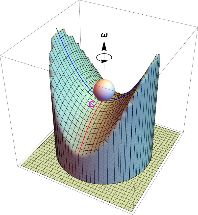
Figure 7: A ball put to the point $C$ will fall under the slightest perturbation when the saddle is fixed, but its position will be stabilized when the saddle is rotated.

Lukash gravitational waves were proposed to study anisotropic models LukashJETP75 ; SiklosAll ; Collins . Their profile in (II.9) is reminiscent of but still different from (in fact more complicated) than that of CPP waves, (II.5). They were studied in Lukash-I along the lines set out by Siklos SiklosAll in the parameter domain (II.38), where they are of Bianchi type VII_h. In this paper we consider instead what happens in the adjacent but different range, (II.27) where problems are solved using different techniques, but, reassuringly, the results agree on the boundary, (II.31), which separates the parameter ranges.

One of our main results here is that the time redefinition (II.13) relates CPP and Lukash waves schematically as,

$$\text{Lukash}\equiv\text{CPP}\;+\;\text{linear force term}\,.$$ (VI.1)

Then a sequence of clever transformations carries the time-dependent Sturm-Liouville problem to a system with constant coefficients, (II.16) - (II.17) , we solve by chiral decomposition Plyuchir ; IonGW . Our results confirm that particles can, in a suitable range of parameters, be trapped by Lukash waves, as shown in figs.2, 3, 4, 5. Bounded geodesics arise when the wave is of Bianchi type VI. The approximations used by Bialynicki-Birula and Charzynski lead to equations similar to our (II.16).

Our findings are exact in two respects :

• We deal with exact plane gravitational waves, and do not use any weak field approximation.

• We solve the equations of motion exactly.

Our time redefinition (II.13) fits into the framework advocated by Gibbons GWG_Schwarzian . Introducing new coordinates $(T,\bm{\xi})$ by,

$$U=f(T),\qquad{\bf X}=\Big{(}\frac{df}{dT}\Big{)}^{1/2}\,\bm{\xi}$$ (VI.2)

extends the trick used in JunkerInomata ; ZZH ; Silagadze in $d=1$ space dimension. Completing (II.13) by (III.3) yields a conformal map between the perturbed CPP (II.1)-(II.2)-(II.5) to Lukash, $ds_{L}^{2}\leftrightarrow d{\Sigma}^{2}$, with conformal factor $\Omega^{2}(U)=e^{T}$. This explains why (II.13) works : conformally related space-times have, up to reparametrization, identical null geodesics.

As an additional bonus, the CPP $\leftrightarrow$ Lukash relation allows us to derive the symmetries of Lukash from those of CPP exactsol ; Ehlers ; POLPER . The additional 6th isometry (IV.5) we call “screw” is reproduced by following backwards our “road map” outlined. in sec. II.2 and summarized, again schematically, by

$$({\bf X},U,V)\quad\leftrightarrow\quad(\bm{\xi},T,\nu)\quad\leftrightarrow\quad(\binom{\alpha}{\beta},T,\nu)\,.$$ (VI.3)

In our examples in sec.V the respective manifolds are conformally related, — however being bounded or not is not invariant under a conformal redefinition of time, (VI.2)  : it is a coordinate dependent statement.

- (1) I. Bialynicki-Birula and S. Charzynski, “Trapping and guiding bodies by gravitational waves endowed with angular momentum,” Phys. Rev. Lett. 121 (2018) no.17, 171101 doi:10.1103/PhysRevLett.121.171101 [arXiv:1810.02219 [gr-qc]].
- (2) H. Stephani, D. Kramer, M. A. H. MacCallum, C. Hoenselaers and E. Herlt, “Exact solutions of Einstein’s field equations,” Cambridge Univ. Press (2003). doi:10.1017/CBO9780511535185
- (3) V. N. Lukash, Sov. Phys. JETP, 40 (1975) 792. “Gravitational waves that conserve the homogeneity of space” Zh. Eksp. Teor. Fiz. 67 (1974) 1594-1608 Sov. Phys. JETP, 40 (1975) 792 . “Some peculiarities in the evolution of homogeneous anisotropic cosmological models,” Astr. Zh. 51, 281 (1974) . “Physical Interpretation of Homogeneous Cosmological Models,” Il Nuovo Cimento 35 B, 208 (1976)
- (4) I. Bialynicki-Birula, “Particle beams guided by electromagnetic vortices: New solutions of the Lorentz, Schrodinger, Klein-Gordon and Dirac equations,” Phys. Rev. Lett. 93 (2004), 020402 doi:10.1103/PhysRevLett.93.020402 [arXiv:physics/0403078 [physics]].
- (5) A. Ilderton “A double copy of the vortex,” Physics Letters B 782 (2018) 22-27 https://doi.org/10.1016/j.physletb.2018.04.069 e-Print: 1707.06821 [physics.plasm-ph]
- (6) I. Bialynicki-Birula and Z. Bialynicka-Birula, “Gravitational waves carrying orbital angular momentum,” New J. Phys. 18 (2016) no.2, 023022 doi:10.1088/1367-2630/18/2/023022 [arXiv:1511.08909 [gr-qc]].
- (7) P. M. Zhang, C. Duval, G. W. Gibbons and P. A. Horvathy, “Velocity Memory Effect for Polarized Gravitational Waves,” JCAP 1805 (2018) 030 doi:10.1088/1475-7516/2018/05/030 [arXiv:1802.09061 [gr-qc]].
- (8) P.-M. Zhang, M. Cariglia, C. Duval, M. Elbistan, G. W. Gibbons and P. A. Horvathy, “Ion traps and the memory effect for periodic gravitational waves,” Phys. Rev. D 98 (2018) 044037 doi:10.1103/PhysRevD.98.044037 [arXiv:1807.00765 [gr-qc]].
- (9) J. Ehlers and W. Kundt, “Exact Solutions of Einstein’s Field Equations,” in L. Witten ed. Gravitation an introduction to current research. Wiley, New York and London (1962)
- (10) H. Bondi, F. A. E. Pirani and I. Robinson, “Gravitational waves in general relativity. 3. Exact plane waves,” Proc. Roy. Soc. Lond. A 251 (1959) 519.
- (11) J-M. Souriau, “Ondes et radiations gravitationnelles,” Colloques Internationaux du CNRS No 220, pp. 243-256. Paris (1973).
- (12) J.-M. Lévy-Leblond, “Une nouvelle limite non-relativiste du group de Poincaré,” Ann. Inst. H Poincaré 3 (1965) 1;
- (13) C. Duval, G. W. Gibbons, P. A. Horvathy and P. M. Zhang, “Carroll symmetry of plane gravitational waves,” Class. Quant. Grav. 34 (2017) no.17, 175003 doi:10.1088/1361-6382/aa7f62 [arXiv:1702.08284 [gr-qc]].
- (14) C. Klein, “Binary black hole spacetimes with a helical Killing vector,” Phys. Rev. D 70 (2004), 124026 doi:10.1103/PhysRevD.70.124026 [arXiv:gr-qc/0410095 [gr-qc]].
- (15) R. Sippel and H. Goenner, “Symmetry classes of pp-waves,” Gen. Rel. Grav. 18, 1229 (1986). D. Eardley, J. Isenberg, J. Marsden and V. Moncrief, “Homothetic and Conformal Symmetries of Solutions to Einstein’s Equations,” Commun. Math. Phys. 106 (1986) 137. doi:10.1007/BF01210929. R. Maartens and S. D. Maharaj, “Conformal symmetries of pp waves,” Class. Quant. Grav. 8 (1991) 503. doi:10.1088/0264-9381/8/3/010.
- (16) P.-M. Zhang, M. Cariglia, M. Elbistan, P. A. Horvathy, “Scaling and conformal symmetries for plane gravitational wave,” J. Math. Phys. 61, 022502 (2020) DOI: 10.1063/1.5136078. [arXiv:1905.08661 [gr-qc]].
- (17) M. Elbistan, P. M. Zhang, G. W. Gibbons and P. A. Horvathy, “Lukash plane waves, revisited,” JCAP 01 (2021), 052 doi:10.1088/1475-7516/2021/01/052 [arXiv:2008.07801 [gr-qc]].
- (18) G. W. Gibbons, “Dark Energy and the Schwarzian Derivative,” [arXiv:1403.5431 [hep-th]].
- (19) M. Elbistan, N. Dimakis, K. Andrzejewski, P. A. Horvathy, P. Kosinski and P. M. Zhang, “Conformal symmetries and integrals of the motion in pp waves with external electromagnetic fields,” Annals Phys. 418 (2020), 168180 doi:10.1016/j.aop.2020.168180 [arXiv:2003.07649 [gr-qc]].
- (20) S. T. C. Siklos, “Some Einstein spaces and their global properties,” J. Phys. A: Math. Gen. 14 (1981) 395-409. “Einstein’s Equations and Some Cosmological Solutions,” in eds. X. Fustero and E. Veraguer Relativistic Astrophysics and Cosmology, Proceedings of the XIVth GIFT International Seminar on Theoretical Physics, p. 201-248. World Scientic (1984). “Stability of spatially homogeneous plane wave spacetimes. I,” Class. Quant. Grav. 8 (1991) 1567-1604.
- (21) C. B. Collins and S. W. Hawking, “Why is the Universe isotropic ?” Astrophys. J. 180 (1973) 317. doi:10.1086/151965 “The rotation and distortion of the Universe,” Mon. Not. Roy. Astron. Soc. 162 (1973) 307.
- (22) L. P. Eisenhart, “Dynamical trajectories and geodesics”, Annals Math. 30 591-606 (1928) C. Duval, G. Burdet, H. Kunzle, M. Perrin, “Bargmann structures and Newton-Cartan theory,” Phys. Rev. D 31 (1985) 1841.
- (23) C. Duval, G.W. Gibbons, P. Horvathy, “Celestial mechanics, conformal structures and gravitational waves,” Phys. Rev. D43 (1991) 3907. [hep-th/0512188].
- (24) P. D. Alvarez, J. Gomis, K. Kamimura and M. S. Plyushchay, “Anisotropic harmonic oscillator, non-commutative Landau problem and exotic Newton-Hooke symmetry,” Phys. Lett. B 659 (2008) 906 doi:10.1016/j.physletb.2007.12.016 [arXiv:0711.2644 [hep-th]]; “(2+1)D Exotic Newton-Hooke Symmetry, Duality and Projective Phase,” Annals Phys. 322 (2007) 1556 doi:10.1016/j.aop.2007.03.002 [hep-th/0702014].
- (25) W. Paul, “Electromagnetic Traps for charged and neutral particles.” Nobel Lecture (1989). Rev. Mod. Phys. 62 (1990) 531. doi:10.1103/RevModPhys.62.531
- (26) O. N. Kirillov and M. Levi, “Rotating saddle trap as Foucault’s pendulum,” Am. J. Phys. 84 (2016), 26-31 doi:10.1119/1.4933206 [arXiv:1501.03658 [physics.class-ph]]. “A Coriolis force in an inertial frame,” Nonlinearity, 30 (2017) 1109-1119. DOI: 10.1088/1361-6544/aa59a0 [arXiv:1509.06703 [math-ph]]
- (27) R. M. Wald, “General Relativity,” doi:10.7208/chicago/9780226870373.001.0001
- (28) C. G. Torre, “Gravitational waves: Just plane symmetry,” Gen. Rel. Grav. 38 (2006) 653 [gr-qc/9907089].
- (29) P. M. Zhang, M. Elbistan, G. W. Gibbons and P. A. Horvathy, “Sturm–Liouville and Carroll: at the heart of the memory effect,” Gen. Rel. Grav. 50 (2018) no.9, 107 doi:10.1007/s10714-018-2430-0 [arXiv:1803.09640 [gr-qc]].
- (30) G. W. Gibbons and C. N. Pope, “Kohn’s Theorem, Larmor’s Equivalence Principle and the Newton-Hooke Group,” Annals Phys. 326 (2011) 1760 doi:10.1016/j.aop.2011.03.003 [arXiv:1010.2455 [hep-th]]; P. M. Zhang, P. A. Horvathy, K. Andrzejewski, J. Gonera and P. Kosinski, “Newton-Hooke type symmetry of anisotropic oscillators,” Annals Phys. 333 (2013) 335 [arXiv:1207.2875 [hep-th]].
- (31) U. Niederer, “The maximal kinematical invariance group of the harmonic oscillator,” Helv. Phys. Acta 46 (1973), 191-200 PRINT-72-4208.
- (32) P. M. Zhang, G. W. Gibbons and P. A. Horvathy, “Kohn’s theorem and Newton-Hooke symmetry for Hill’s equations,” Phys. Rev. D 85 (2012), 045031 doi:10.1103/PhysRevD.85.045031 [arXiv:1112.4793 [hep-th]].
- (33) L. Hsu and J. Wainwright, “Self similar spatially homogeneous cosmologies: Orthogonal perfect fluid and vacuum solutions,” Class. Quant. Grav. 3 (1986), 1105-1124 doi:10.1088/0264-9381/3/6/011
- (34) G. Junker and A. Inomata, “Transformation of the free propagator to the quadratic propagator,” Phys. Lett. A 110 (1985) 195-198
- (35) Q. L. Zhao, P. M. Zhang and P. A. Horvathy, “Time-dependent conformal transformations and the propagator for quadratic systems,” [arXiv:2105.07374 [quant-ph]].
- (36) K. Andrzejewski and S. Prencel, “Memory effect, conformal symmetry and gravitational plane waves,” Phys. Lett. B 782 (2018), 421-426 doi:10.1016/j.physletb.2018.05.072 [arXiv:1804.10979 [gr-qc]]. “Niederer’s transformation, time-dependent oscillators and polarized gravitational waves,” doi:10.1088/1361-6382/ab2394 [arXiv:1810.06541 [gr-qc]].
- (37) S. Dhasmana, A. Sen and Z. K. Silagadze, “Equivalence of a harmonic oscillator to a free particle and Eisenhart lift,” Annals Phys. 434 (2021), 168623 doi:10.1016/j.aop.2021.168623 [arXiv:2106.09523 [quant-ph]].
- (38) P. A. M. Dirac, “New basis for cosmology,” Proc. Roy. Soc. Lond. A 165 (1938), 199-208 doi:10.1098/rspa.1938.0053
- (39) see, e.g. M. Blau, Lecture Notes on General Relativity, http://www.blau.itp.unibe.ch/GRLecturenotes.html