Conservation with moving meshes over orography
Abstract
Adaptive meshes have the potential to improve the accuracy and efficiency of atmospheric modelling by increasing resolution where it is most needed. Mesh re-distribution, or r-adaptivity, adapts by moving the mesh without changing the connectivity. This avoids some of the challenges with h-adaptivity (adding and removing points): the solution does not need to be mapped between meshes, which can be expensive and introduces errors, and there are no load balancing problems on parallel computers. A long standing problem with both forms of adaptivity has been changes in volume of the domain as resolution changes at an uneven boundary. We propose a solution to exact local conservation and maintenance of uniform fields while the mesh changes volume as it moves over orography. This is solved by introducing a volume adjustment parameter which tracks the true cell volumes without using expensive conservative mapping.
A finite volume solution of the advection equation over orography on moving meshes is described and results are presented demonstrating improved accuracy for cost using moving meshes. Exact local conservation and maintenance of uniform fields is demonstrated and the corrected mesh volume is preserved.
We use optimal transport to generate meshes which are guaranteed not to tangle and are equidistributed with respect to a monitor function. This leads to a Monge-Ampère equation which is solved with a Newton solver. The superiority of the Newton solver over other techniques is demonstrated in the appendix. However the Newton solver is only efficient if it is applied to the left hand side of the Monge-Ampère equation with fixed point iterations for the right hand side.
keywords: moving meshes; mesh re-distribution; r-adaptivity; numerical weather prediction; orography
1 Introduction
Dynamic mesh adaptivity can be advantageous for the numerical solution of PDEs when numerical errors (or their impacts) are greater in some areas than others. Numerical weather and climate predictions, for example, could be improved by locally varying the spatial resolution through time, tracking atmospheric phenomena such as weather fronts Budd et al. (2013).
-adaptivity involves adding and removing computational points based on local resolution requirements (e.g. Berger and Oliger, 1984; Skamarock and Klemp, 1993; Weller, 2009). The connectivity of the mesh and the total number of computational points change. Conversely, -adaptivity, or mesh re-distribution, involves moving mesh vertices without changing the connectivity of the mesh. It results in a deformed mesh keeping the number of computational points and topology the same (e.g. Dietachmayer and Droegemeier, 1992; Hirt et al., 1997; Kühnlein et al., 2012).
-adaptivity is an attractive form of adaptivity since the data structures associated with the connectivity do not change and therefore the load balancing remains constant on parallel computers. -adaptivity does not require mapping solutions between old and new meshes. -adaptivity can also lead to smoothly graded meshes, which are desirable in order to reduce wave reflections and other errors associated with rapid resolution changes (Vichnevetsky, 1987; Long and Thuburn, 2011).
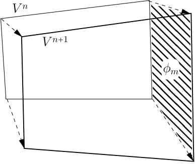
A disadvantage of -adaptivity is, with a fixed number of points and fixed connectivity, it is not possible to achieve exactly the required resolution in each direction simultaneously, which can be achieved with -adaptivity. This causes an extra difficulty when introducing orography. For example, we consider a vertical slice model with a horizontally moving mesh over orography (Figure 1). When the topographic surface is approximated as piecewise linear (or higher order) splines based on vertex locations, the shape of orography inevitably changes as mesh vertices move over the orography. Therefore the volume of the domain changes as the mesh moves, which results in unphysical compression or expansion of the model fluid.
With -adaptivity, this issue can be avoided by evaluating all the metric terms from orography on the finest grid everywhere in the domain and average the result, in a consistent manner, to any coarser grid (Guzik et al., 2015). This approach is only suitable for models in which each fine grid cell only ever over-laps with one coarse grid cell. Another way to resolve this issue is using conservative mapping to calculate the cell volumes over the original shape of orography. For example, Schwartz et al. (2015) presented an algorithm to perform highly accurate mappings using sub-grid knowledge, which ensures the required accuracy with grid refinement. Though this approach can be used with both - and -adaptivities, it is expensive to perform conservative mapping of the orography every time step.
Instead of tracking the shape of orography within each cell, we propose another solution which is to calculate the “true” cell volumes indirectly by solving a transport equation for the cell volume. This is solved by introducing a volume adjustment parameter which tracks the change in cell volumes caused by the change in the shape of orography. With this approach, the exact local conservation and maintenance of uniform fields on a moving mesh over orography is achieved without using expensive conservative mapping.
Section 2 provides the model description, including the finite-volume discretisation on a moving mesh, and the adjustment of the cell volumes as mesh moves over orography. In section 3, we present the results of a three-dimensional tracer advection test with the use of the volume adjustment parameter. Here we evaluate the model error using smooth and steep orography and demonstrate the importance of maintaining uniform fields on a moving mesh. Finally, in section 4 we provide a summary and outlook. We prove that the method for calculating adjusted cell volumes is bounded in appendix A and we describe the optimally transported mesh generation in appendix B.
2 Model Description
2.1 Finite volume discretisation on a moving mesh
We consider the three-dimensional advection equation in flux form:
| (1) |
where is a prescribed velocity field and is the tracer density. To derive a finite-volume descretised equation, first we integrate the equation over a control volume and then apply Gauss’ divergence theorem:
| (2) |
where is the outward pointing unit normal vector on the boundary surface of the control volume so that is the flux of over the surface with area . To extend (2) to a moving mesh, we use the Reynolds transport theorem:
| (3) |
where is the velocity of the boundary surface . Note that the control volume and the boundary surface are now time dependent. The relationship between the volume and the velocity is called the space conservation law (Demirdžić and Perić, 1988):
| (4) |
This means that the change in the control volume has to match the sum of the swept volumes of all its surfaces. Combining the equations (2) and (3), we have the integral form of the advection equation (1) on a moving mesh:
| (5) |
The discretised form of the equation (5) can be written:
| (6) |
where values inside the summation are at time step , is the time step size, denotes the tracer density that is interpolated onto the cell faces, and is the face flux defined on the cell faces. The mesh flux is calculated as the swept volume by the faces during each time step (Figure 2), which satisfies the following discretised form of the equation (4):
| (7) |
2.2 Automatic mesh motion
The optimally transported mesh generation procedure is described in appendix B. The Monge-Ampère equation is solved to generate a mesh that is equidistributed with respect to a monitor function and guaranteed tangle free due to the optimal transport. A Newton method is described to solve the Monge-Ampère equation. A monitor function is chosen so that the cell areas are a factor of 4 smaller in regions where the second derivatives of the tracer density is highest compared with the regions of lowest second derivatives. The mesh is moved every time step so fast convergence of the Newton solver is important, which is also demonstrated in appendix B.
2.3 Volume adjustment as mesh moves over orography
When the cell volumes are calculated from vertex locations without tracking the variations in orography within each cell, the shape of the model orography inevitably changes as the mesh vertices move (Figure 1). This means that equation (7) does not hold on a moving mesh over orography: we only consider the swept volumes in the horizontal, not the swept volume of the orography surface. The mismatch between the change in the control volume and the sum of the swept volumes results in non-uniform model fields at the bottom surface.
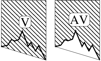
One solution to this problem would be to use a conservative mapping of old to new mesh to calculate the cell volumes over the original shape of orography (hereafter the “true cell volumes”). However we want to avoid the expense of conservative mapping every time step, particularly as we are only interested in the true cell volumes and not in the shape of orography itself. Therefore, instead of tracking the shape of orography within each cell, we track the true cell volumes by solving the following advection equation for a cell volume:
| (8) |
where is the volume adjustment parameter and is the volume of cells as defined only by their vertices so that corresponds to the true cell volumes (Figure 3). To avoid having negative cell volumes, we use a downwind value of , denoted by , in the right-hand side. This guarantees that is always positive as long as the initial value of is positive at all cells (see appendix A for a proof). Then we use in the advection equation (6) instead of and solve it using a two stage Runge-Kutta method with an off-centring parameter :
| (9) | |||||
| (10) |
where the mesh flux is evaluated at time step as in Figure 2. In this way, we achieve conservation of both the total of the true cell volume (i.e., the total ) and the total mass relative to the true domain size (i.e., the total ), thereby maintaining uniform fields without the need to track the shape of orography within each cell.
To prove that our scheme preserves a uniform field on a moving mesh, we assume a divergence free velocity field so that for each cell
| (11) |
at all time steps, and check if the solution stays uniform when the initial condition is uniform. Given , the equation (9) becomes
| (12) |
Substituting the equations (8) and (11) into (12), we have
| (13) |
As , we obtain . Then the equation (10) becomes
| (14) |
In the same way as above, we obtain . Therefore it is proved that the solution stays uniform in a divergence-free velocity field when the initial condition is uniform. In section 3, we will confirm this result numerically, whereas the model without the volume adjustment suffers from artificial compression and expansion of the fluid in association with the mesh movement over orography.
2.4 Advection scheme
Section 2.1 describes the interaction of the discretisation with the moving mesh, and section 2.3 includes the description of a two-stage, second-order Runge-Kutta time stepping scheme as in the equations (9) and (10). To complete the discretisation we must specify how face values, , are calculated from cell values, . We use a simple, second-order linear upwind advection scheme without monotonicity constraints. The use of an unbounded advection scheme makes it easier to ensure that the mesh motion over orography does not generate spurious oscillations. The face values are approximated as:
| (15) |
where is the value of in the cell upwind of the face, is the vector that goes from the upwind cell centre to the face centre, and is the gradient of calculated in the upwind cell using Gauss’ divergence theorem:
| (16) |
where is the values of linearly interpolated from cell centres onto faces and is the outward pointing vector normal to each face with magnitude equal to the face area (the face area vector).
3 Results
3.1 Advection over smooth orography
In this section, we present the results of an advection test on a three-dimensional mesh with one layer in the vertical direction. We use a computational domain with a size of , where the domain half-length and height are set to 5 km and 1 km, respectively. The number of cells is both in the and directions. All boundaries of the domain are considered as a rigid wall.
(a)

(b)

(a)
(b)

(a)
(b)
(c)
(d)

(a)
(b)
(c)
(d)
(a)

(b)


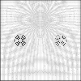
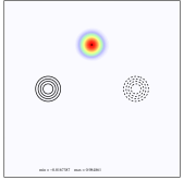
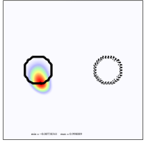
A bubble of tracer is transported by a solid body rotating velocity field. Figure 4 shows diagrams of the tracer density and the velocity of the initial state. The initial tracer density is defined as
| (17) | ||||
| (18) |
where the tracer radius , and the distance to the centre of the tracer,
| (19) |
with the centre of the tracer initially at . The non-divergent velocity field can be written in terms of a stream function as
| (20) |
and . We use that yields a velocity field which rotates around the centre of the domain and decays linearly to zero before it reaches the boundaries:
| (21) | ||||
| (22) | ||||
| (23) |
where is the distance to the centre of the domain. The inner radius is set to so that the tracer is separate from the sheared velocity and the outer radius is set to so that the velocity is zero at the boundary. The angular velocity is given by s-1 so that the tracer is transported counterclockwise and reaches its initial position after 600 seconds. Note that the velocity field is recalculated after every time step so that it is always non-divergent on a moving mesh.
The tracer passes over a hill and a valley, as shown in Figure 5, with surface height given by
| (24) | ||||
| (25) | ||||
| (26) |
where is the orography radius, m is the height at the centre of the hill and that of the valley m. The distance to the centre of the hill with , and the distance to the centre of the valley with .
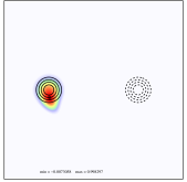
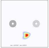
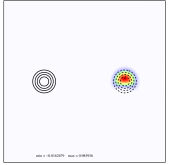
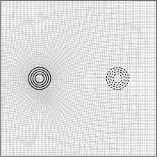
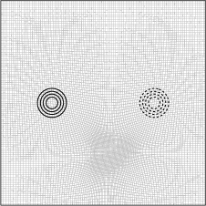
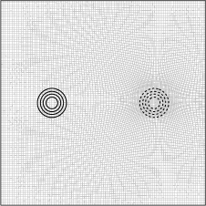
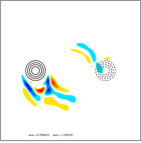
First we present results from the control run, where the number of cells 100 and the time step = 0.5 s are used. Figures 6 and 7 show four snapshots of the tracer density and the moving mesh, respectively, at t = 150 s, 300 s, 450 s and 600 s. As the velocity field is non-divergent, the tracer is accelerated over the hill and decelerated over the valley, returning to its original shape and position after 600 s. The mesh successfully tracks the tracer as it moves and changes its shape, without tangling. As described in section 2.2, the monitor function is chosen here so that the cell areas are a factor of 4 smaller in regions where the second derivatives of the tracer density is highest compared with the regions of lowest second derivatives (see appendix B.3 for details).
(a)
(b)
(c)


(a)
(b)

Figure 8 shows the conservation errors in the total cell volumes and the total mass. While the numerical domain size (the total ) changes as the mesh moves, the true domain size (the total ) stays constant (Figure 8a). At the same time, the model conserves the total mass relative to the true domain size (the total ), as shown in Figure 8b, achieving exact local conservation and maintenance of uniform fields at the bottom boundary. Figure 9 shows the variation of maximum and minimum values of in the domain for the period of 10 revolutions. It demonstrates that the first-order downwind differencing of ensures that is always positive, thereby the model may not have negative cell volumes.
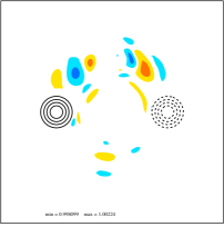
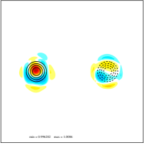
To demonstrate that the model maintains uniform fields as mesh moves over orography, we repeat the experiment using a uniform field instead of using the cosine-shaped tracer. Here we compare the results with and without the use of the volume adjustment parameter . Figures 10a and 10b show the density fields at 150 s and 600 s, respectively, when is not used in the model. The results show evidence of artificial compression and expansion of the model fluid in association with the mesh movement over orography. On the other hand, the density field stays constant at 1 throughout the period of 600 s when is used to adjust the cell volumes (Figure 10c). Figures 11a and 11b show snapshots of the field at 150 s and 600 s, respectively. These results demonstrate that successfully tracks the changes in the cell volumes over orography and adjusts the cell volumes so that the total of the true cell volumes as well as the total mass in the true domain is conserved, thereby maintaining uniform fields as the mesh moves over orography.
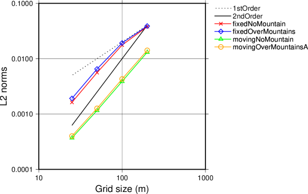
Finally, Figure 12 shows a log-log plot of the norm of the errors in versus the grid size after one complete revolution, alongside the theoretical first- and second-order convergence rates. Time steps of 1 s, 0.25 s and 0.125 s are used for the cases of 50, 200 and 400, respectively. The same cosine-shaped tracer as in the control run is used here at all resolutions. At each resolution, errors are calculated both on the fixed uniform mesh and the moving mesh, with and without the orography at the bottom surface. The model shows the convergence rate of 1.70 on the uniform mesh over orography and that of 1.58 on the moving mesh over orography. It is shown that the implementation of orography doesn’t affect the order of convergence both on the uniform mesh and the moving mesh. The convergence rate on the moving mesh could be improved by optimising the monitor function or using a higher-order advection scheme, but it is outside the scope of this paper.
3.2 Advection over steep orography
In the previous section, we performed a tracer advection test and showed that our scheme maintains a uniform field on a moving mesh over orography, using smooth hill and valley as shown in Figure 5 as a sample orography. In this section, we demonstrate the importance of the maintenance of uniform fields by repeating the tracer advection test using a pair of cylinder-shaped hill and valley which has steep cliffs on the sides, with surface height given by
| (27) | ||||
| (28) | ||||
| (29) |
where m. All the other simulation setup is the same as that of the control run in the previous section. We run the model with and without the use of the volume adjustment parameter and compare the results.
(a)
(b)

(a)
(b)

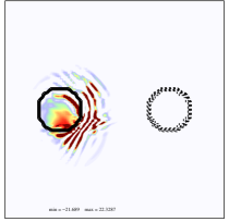
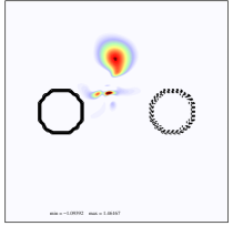
Figure 13 shows the density fields at t = 150 s and t = 600 s when is not used in the model. Large numerical errors are found when the tracer passes over the hill (Figure 13a), and the tracer doesn’t recover its original shape after one complete revolution (Figure 13b). It might be possible to dampen the oscillations in the solution with an aggressive monotonic advection scheme but monotonic advection should only be achieved for non-divergent wind fields whereas we have introduced artificial divergence by changing the mesh volume. These oscillations should be prevented from occurring by treating the mesh volume correctly. Figure 14 shows the results when is used to adjust the cell volumes in the model. In this case, the tracer successfully passes over the hill (Figure 14a) and valley, and completes the revolution without losing shape (Figure 14b). Therefore it is shown that the inclusion of in the model yields stable solutions over steep orography while we observe substantial errors in the model without A, thereby showing the importance of the maintenance of uniform fields on a moving mesh over orography.
4 Conclusion
We proposed a novel approach to solve the problem of changes in volume of the domain when resolution changes over orography in a simulation using adaptive meshes. The volume adjustment parameter is introduced which tracks the true cell volumes by solving an advection equation for a cell volume, achieving conservation of both the volume of the domain and the total mass without tracking the shape of orography within each cell. The results of a three-dimensional tracer advection test showed that our scheme maintains a uniform field while the mesh resolution changes over orography, whereas the model without the volume adjustment suffers from artificial compression and expansion of the fluid due to the lack of conservation in volume of the domain. The importance of the maintenance of uniform fields was demonstrated over steep orography where the change in cell volumes on a moving mesh can be pronounced without volume adjustment. The resulting artificial changes in volume lead to large unbounded errors when the advected tracer moves over orography. The volume adjustment parameter successfully avoided the errors by efficiently tracking the changes in the cell volumes over orography and adjusting the cell volumes. The same idea is considered to be applicable to other variable boundary conditions on a moving mesh (e.g. a land sea mask). Further work is intended to apply this method to the shallow water or fully compressible equations with the aim of simulating atmospheric problems on a moving mesh over real orography.
Acknowledgement
We would like to acknowledge NERC grant NE/M013693/1. The source code for this project is located at https://github.com/AtmosFOAM/AMMM with the tag paper.2021; the simulation code itself is located within this repository under run/advection/advectionOTFoam/advectionOT/runAll. The codes are developed with OpenFOAM 7 (https://openfoam.org, 2019).
Appendix A Boundedness of Volume Adjustments
In section 2.3, we introduced a volume adjustment parameter, , to correct the cell volumes, , calculated from vertex locations sampled over orography. As the mesh moves, the sum of all changes but the sum of does not change. Here we prove that is bounded above zero which is needed to guarantee that the model may not have negative cell volumes.
The parameter is calculated from an advection equation (8) discretised using first-order forward in time and first-order downwind in space, which can be rewritten as:
| (30) | |||||
where denotes the tracer density at the neighbouring cell downstream. This can be re-arranged for as a function of values of at time level :
| (31) |
Given that and , we can see that when
| (32) |
Since the courant number is defined as
| (33) |
if . Therefore it is proved that, when the initial value of is positive at all cells, stays positive as long as the Courant number is less than one.
Appendix B Numerical Solution of the Monge-Ampère Equation for Mesh Generation
The meshing technique is described in full, analysed and compared with other methods full in Browne et al. (2016) which is summarised here and results are presented for the meshes used in this paper.
B.1 Introduction
An optimally transported mesh is as close as possible to the original mesh (close being defined by the root mean square distance between the vertices of the original and transported mesh) whilst equidistibuting a given scalar monitor function Budd and Williams (2009). To guarantee that the transported mesh is not tangled, the locations, , are defined from the locations of the original mesh, , by the addition of the gradient of a mesh potential, :
| (34) |
Equidistribution of the monitor function, is expressed as:
| (35) |
for a constant uniform across space where is the matrix determinant. The combination of equations (34) and (35) gives a fully non-linear elliptic PDE, the Monge-Ampère equation:
| (36) |
where is the identity tensor and is the Hessian. The meshes in this paper are all the result of numerical solution of the Monge-Ampére equation.
Budd and Williams (2009) added Laplacian smoothing and a rate of change term to (36) making it parabolic and solved using a spectral method. Weller et al. (2016) derived an equation to generate optimally transported meshes on the surface of a sphere, linearised about a uniform flat mesh to create fixed point iterations, each iteration requiring the solution of a Poisson equation discretised using finite volumes. McRae et al. (2018) re-wrote the equation on the surface of a sphere as a PDE and solved using a Newton solver with finite elements. Here we describe a Newton method for solving the Monge-Ampère equation on a finite plane and discretise in space with finite volumes following Weller et al. (2016).
B.2 Numerical Method
We define a Newton method for solving (36) in Euclidean geometry, linearising the LHS around the previous iteration and using the RHS from the previous iteration. is the solution at iteration . By writing it can be shown that
| (37) |
where is the matrix of cofactors of and is some nonlinear function. In 2D
| (38) |
and . In 3D, a more involved calculation can show and
At convergence terms proportional to (where is the dimensionality of space) will disappear so at each iteration, we solve the following Poisson equation for :
| (39) |
Equation (39) is elliptic as long as is positive definite. For simplicity and efficiency we use a finite volume discretisation for spatial discretisation of (39). However, unlike wide stencil finite difference methods (e.g. Oberman, 2008), this is not guaranteed to give monotonic solutions . This means that can become non-positive definite so (39) loses its ellipticity and solutions rapidly diverge. To remedy this we can modify (39) to maintain ellipticity by replacing the matrix with a modified matrix such that
| (40) |
and is defined as
| (41) |
The constant is chosen to avoid round-off errors (we have taken ), and refers to the spectrum of . This process simply shifts the eigenvalues of the matrix so that they remain positive.
The iterations labelled are called outer iterations because the Poisson equation is also solved using an iterative solver within each outer iteration.
The Laplacian and the Hessian of (39) are discretised in space using compact finite volumes, following Weller et al. (2016). This is equivalent to second order finite differences on a uniform grid. Zero gradient boundary conditions are used. The spatial discretisation leads to a set of linear simultaneous equations. These are solved using the OpenFOAM GAMG solver with a symmetric Gauss Seidel smoother and an LU pre-conditioner. A maximum of 10 solver iterations are allowed. The tightest solver tolerance is but the solver is only solved to a tolerance of 0.01 times the initial residual each outer iteration. This is to avoid spending too much time solving the first few iterations tightly when subsequent iterations will have updated coefficients.
B.3 The Monitor Function
The monitor function is based on the Frobenius norm of the Hessian of the tracer density, , which in two dimensions is
| (42) |
Following McRae et al. (2018) we use the rule of thumb that half of the resolution should be placed where not much is happening. This can be approximately achieved by setting:
| (43) |
where is the area average of and is the ratio of smallest to largest cell volumes/areas of the resulting adapted mesh. For the simulations in section 3 we use meaning that, if cells have aspect ratio 1 then the maximum ratio of smallest to largest cell side lengths is 2. The monitor function is smoothed before it is used for mesh generation so that the resulting mesh varies smoothly, which is advantageous for finite volume and finite difference methods that have the property of super convergence. The final monitor function, , is the implicit solution of the diffusion equation:
| (44) |
where the diffusion coefficient, , is mesh size and time step dependent:
| (45) |
is equivalent to the number of applications of a filter to smooth the monitor function. is used for the meshes presented in section 3. The Laplacian in (44) is calculated on the uniform orthogonal computational mesh of squares using 2nd-order centred differences (i.e. differencing in each direction).
B.4 Results
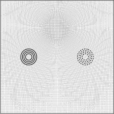
Meshes are generated for the linear advection results using a cosine-shaped tracer in section 3.1 starting from initial uniform grids of , , and points in a plane of size 10 km by 10 km.
| Convergence of mesh generation starting from regular mesh | |
|---|---|
 |
 |
| Convergence of mesh generation each time step | |
 |
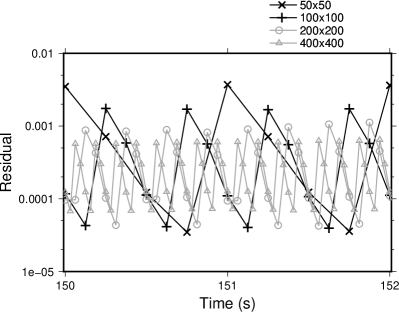 |
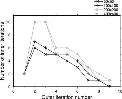
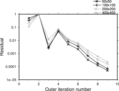
Before the advection simulation starts, an initial mesh is generated using the monitor function calculated from the analytic description of the initial conditions. 9 outer iterations are used. The residual of the Poisson equation solver and the number of iterations of the Poisson equation solver for each outer iteration are shown in the top row of Figure 15 for all resolutions. Convergence is reasonably insensitive to resolution which is necessary for efficiency. Convergence in the first three iterations is noisy but then convergence proceeds exponentially (note the residuals are on a log-scale).
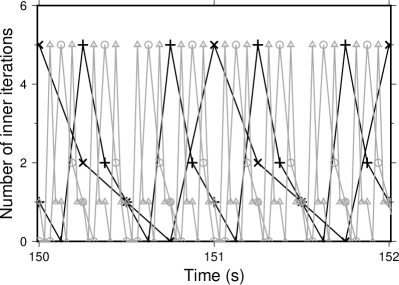
While solving the advection equation, the mesh is moved every time step. The same uniform, regular computational mesh is used to solve the Monge-Ampère equation each time step but the solution is initialised from the previous time step. Each time step, a maximum of 4 outer iterations of the Monge-Ampère Newton solver are allowed. The number of inner (linear equation solver) iterations and the initial residual for each solver are shown in the bottom row of Figure 15. This shows that at most 5 inner iterations are needed and convergence is exponential between each outer-iteration per time step.
B.5 Further Remarks
Section B.2 described a regularisation technique to ensure that the discretised Poisson equation (39) remains elliptic by artificially increasing the diagonal of the Poisson equation coefficient, . This may raise concerns that we are arbitrarily changing the problem that we are solving. However the regularisation is only very occasionally needed and is only ever needed during the first one or two outer iterations and so this regularisation never influences the final converged solution.
Browne et al. (2016) compared this Newton solver with the parabolic method of Browne et al. (2014) and with the fixed point iterations used by Weller et al. (2016). Convergence of the proposed Newton solver was far superior and free of arbitrary parameters. Browne et al. (2016) also proposed a Newton solver that involved linearising the term of (39). This lead to even faster but unreliable convergence and so is not used here.
References
- Berger and Oliger (1984) Berger, M. J., Oliger, J., 1984. Adaptive mesh refinement for hyperbolic partial differential equations. Journal of Computational Physics 53 (3), 484–512.
- Browne et al. (2014) Browne, P., Budd, C., Piccolo, C., Cullen, M., 2014. Fast three dimensional r-adaptive mesh redistribution. Journal of Computational Physics 275, 174–196.
-
Browne et al. (2016)
Browne, P., Prettyman, J., Weller, H., Pryer, T., van Lent, J., 2016. Nonlinear
solution techniques for solving a monge-ampère equation for redistribution
of a mesh. arXiv Numerical Analysis arXiv:1609.09646.
URL https://arxiv.org/abs/1609.09646 - Budd et al. (2013) Budd, C. J., Cullen, M., Walsh, E., 2013. Monge–ampére based moving mesh methods for numerical weather prediction, with applications to the eady problem. Journal of Computational Physics 236, 247–270.
- Budd and Williams (2009) Budd, C. J., Williams, J., 2009. Moving mesh generation using the parabolic monge–ampère equation. SIAM Journal on Scientific Computing 31 (5), 3438–3465.
- Demirdžić and Perić (1988) Demirdžić, I., Perić, M., 1988. Space conservation law in finite volume calculations of fluid flow. International Journal for Numerical Methods in Fluids 8 (9), 1037–1050.
- Dietachmayer and Droegemeier (1992) Dietachmayer, G. S., Droegemeier, K. K., 1992. Application of continuous dynamic grid adaption techniques to meteorological modeling. part i: Basic formulation and accuracy. Monthly Weather Review 120 (8), 1675–1706.
- Guzik et al. (2015) Guzik, S. M., Gao, X., Owen, L. D., McCorquodale, P., Colella, P., 2015. A freestream-preserving fourth-order finite-volume method in mapped coordinates with adaptive-mesh refinement. Computers & Fluids 123, 202–217.
- Hirt et al. (1997) Hirt, C., Amsden, A., Cook, J., 1997. An arbitrary lagrangian–eulerian computing method for all flow speeds. Journal of Computational Physics 135 (2), 203–216.
- Kühnlein et al. (2012) Kühnlein, C., Smolarkiewicz, P. K., Dörnbrack, A., 2012. Modelling atmospheric flows with adaptive moving meshes. Journal of Computational Physics 231 (7), 2741–2763.
- Long and Thuburn (2011) Long, D., Thuburn, J., 2011. Numerical wave propagation on non-uniform one-dimensional staggered grids. Journal of Computational Physics 230 (7), 2643–2659.
- McRae et al. (2018) McRae, A. T. T., Cotter, C. J., Budd, C. J., 2018. Optimal-transport-based mesh adaptivity on the plane and sphere using finite elements. SIAM Journal on Scientific Computing 40 (2), A1121–A1148.
- Oberman (2008) Oberman, A. M., 2008. Wide stencil finite difference schemes for the elliptic monge-ampere equation and functions of the eigenvalues of the hessian. Discrete & Continuous Dynamical Systems-B 10 (1), 221.
- Schwartz et al. (2015) Schwartz, P., Percelay, J., Ligocki, T., Johansen, H., Graves, D., Devendran, D., Colella, P., Ateljevich, E., 2015. High-accuracy embedded boundary grid generation using the divergence theorem. Communications in Applied Mathematics and Computational Science 10 (1), 83–96.
- Skamarock and Klemp (1993) Skamarock, W. C., Klemp, J. B., 1993. Adaptive grid refinement for two-dimensional and three-dimensional nonhydrostatic atmospheric flow. Monthly Weather Review 121 (3), 788–804.
- Vichnevetsky (1987) Vichnevetsky, R., 1987. Wave propagation and reflection in irregular grids for hyperbolic equations. Applied Numerical Mathematics 3, 133–166.
- Weller (2009) Weller, H., 2009. Predicting mesh density for adaptive modelling of the global atmosphere. Philosophical Transactions of the Royal Society of London A: Mathematical, Physical and Engineering Sciences 367 (1907), 4523–4542.
- Weller et al. (2016) Weller, H., Browne, P., Budd, C., Cullen, M., 2016. Mesh adaptation on the sphere using optimal transport and the numerical solution of a monge–ampère type equation. Journal of Computational Physics 308, 102–123.