Improved efficiency of multilevel Monte Carlo
for stochastic PDE through strong pairwise coupling

Abstract.

Multilevel Monte Carlo (MLMC) has become an important methodology in applied mathematics for reducing the computational cost of weak approximations. For many problems, it is well-known that strong pairwise coupling of numerical solutions in the multilevel hierarchy is needed to obtain efficiency gains. In this work, we show that strong pairwise coupling indeed is also important when MLMC is applied to stochastic partial differential equations (SPDE) of reaction-diffusion type, as it can improve the rate of convergence and thus improve tractability. For the MLMC method with strong pairwise coupling that was developed and studied numerically on filtering problems in [Chernov et al., Numer. Math., 147 (2021), 71-125], we prove that the rate of computational efficiency is higher than for existing methods. We also provide numerical comparisons with alternative coupling ideas on linear and nonlinear SPDE to illustrate the importance of this feature.

1. Introduction

The efficiency of numerical methods is a very important topic for practitioners that has lately seen a surge of interest in the field of uncertainty quantification (UQ) [40, 41, 42]. UQ seeks to combine statistical and probabilistic techniques with traditional numerical schemes to improve the modeling and the accuracy of estimates. Examples of applications include climate modeling, subsurface flow, medical imaging and deep learning [1, 12, 37]. A particular focus has been given on the class of numerical methods known as Monte Carlo (MC) methods, which are used to solve problems incorporating elements of randomness or uncertainty [35, 39, 42], i.e., in stochastic computations. One methodology which has exhibited improved efficiency and a high level of applicability, is multilevel Monte Carlo (MLMC).

MLMC is a numerical technique aimed at reducing the computational cost of the Monte Carlo method. The methodology was first introduced by Heinrich [22] and extended and popularized by various works on diffusion processes by Giles [14, 15]. The methodology of MLMC can be viewed as a variance-reduction technique. Since these works, MLMC has been applied in numerous areas, including stochastic filtering [6, 13, 24, 26, 27], Markov chain Monte Carlo (MCMC) [7, 10] and partial differential equations with random input arising in UQ [2, 7, 19]. MLMC is based upon a given problem, such as estimating an expectation at some terminal time, w.r.t. the law of a diffusion process, that requires a discretization. For instance, in the diffusion case, this can be a time-discretization based on the Euler method. One then decomposes an expectation w.r.t. a law associated to a very precise discretization into a telescoping sum of differences of expectations associated to laws of increasingly coarse discretizations. The objective is then to sample from coupled probability distributions associated to consecutive discretized laws and to apply Monte Carlo at each summand of the telescoping sum to achieve a variance reduction, relative to using Monte Carlo at the finest discretization. The amount of discretization refers to the level, in the acronym MLMC.

Despite the substantial advancements made with MLMC, the number of applications and research papers on applying the methodology to stochastic partial differential equations (SPDE) [29] is relatively small. Such examples include finite-difference solvers with applications in mathematical finance [16], and finite element methods for parabolic SPDE [3, 5]. There are open questions on the efficiency and scope of MLMC for SPDE which we use as motivation for this work: is it possible to improve the efficiency of MLMC through strong pairwise coupling of numerical solutions of SPDE, and can that widen the scope of MLMC on SPDE to problems in higher dimensions and with lower-regularity driving noise?

Our objective in this manuscript is to present a complexity study of an alternative way to apply MLMC for SPDE, which can demonstrate computational gains. This approach is based on the exponential Euler method [11, 23, 30, 36] and strong pairwise coupling of solution realizations on different levels. The strong pairwise coupling approach was introduced and studied experimentally in the work on finite-dimensional Langevin SDE by Müller et al. [38] and extended to filtering methods for (infinite-dimensional) SPDE by Chernov et al. [8]. The coupling idea is based on the exponential Euler integrator [11, 23, 33, 36] for time-discretization of reaction-diffusion type SDE/SPDE. For the finite-dimensional SDE in [38], strong coupling is shown to produce constant-factor efficiency gains in numerical experiments, whereas for the herein considered class of SPDE, we show that strong coupling reduces the asymptotic rate of growth in the computational cost. This indicates that strong coupling for MLMC can lead to more substantial asymptotic efficiency gains for infinite-dimensional problems than for finite-dimensional ones.

The main contribution of this work is to demonstrate the improvements of the discussed coupling approach, for numerically solving SPDE. This is presented in the standard-format cost-versus-error result for exponential Euler MLMC in Theorem 3.4. Specifically, our findings suggest that in order to achieve $\mathcal{O}(\epsilon^{2})$ mean squared error (MSE) in a standard setting, we have to pay $\mathcal{O}(\epsilon^{-2})$ in computational cost. This is a reduction in cost compared to other existing methods, such as the Milstein MLMC method, for which the cost is $\mathcal{O}(\epsilon^{-3})$, cf. Theorem 3.6 and [5], and it is, to the best of our knowledge, the first theoretical result on the performance of the exponential Euler MLMC for any nonlinear stochastic PDE. We also verify these gains numerically on two SPDE, one with a linear reaction term and one with a nonlinear one.

The outline of this paper is as follows. In Section 2 we describe our model problem, which is a semilinear SPDE, and review fundamental properties of the MLMC method. Section 3 describes our proposed coupling method for MLMC and two alternative methods. We also summarize the theoretical properties of our main MLMC method in Theorem 3.4. Numerical experiments on various SPDE are conducted in Section 4 to demonstrate the improvement with the proposed coupling. Finally, we conclude our findings, and provide future areas of research, in Section 5. Required model assumptions are provided in the Appendix.

2. Background material

In this section we present and review the MLMC method applied to numerical discretizations of SPDEs. We first introduce the SPDE under consideration, and then review the approximation methods: a spectral Galerkin spatial discretization combined with either exponential Euler or Milstein discretization in time.

2.1. Notation

Let $T>0$ and let $(\Omega,\mathcal{F},\mathbb{P})$ be a complete probability space equipped with a filtration $\mathcal{F}_{t\in[0,T]}$. $H$ denotes a non-empty separable Hilbert space with inner product $\langle\cdot,\cdot\rangle$, norm $\|\cdot\|_{H}=\sqrt{\langle\cdot,\cdot\rangle}$ and orthogonal basis $(e_{n})_{n=1}^{\infty}$. $L^{2}(\Omega,H)$ denotes the associated Bochner–Hilbert space, consisting of the set of strongly measurable maps $f:\Omega\to H$ such that

$$\|f\|_{L^{2}(\Omega,H)}^{2}:=\int_{\Omega}\|f(\omega)\|_{H}^{2}\,\mathrm{d}\mathbb{P}(\omega)<\infty$$

Let $\mathbb{N}:=\{1,2,\ldots\}$, and for every $N\in\mathbb{N}$, we introduce the finite-dimensional subspace $H^{N}:=\textrm{span}\{e_{n}\mid n=1,\dots,N\}\subset H$ and the associated orthogonal projection operator $P_{N}v:=\sum^{N}_{n=1}\langle v,e_{n}\rangle\,e_{n}$ for $v\in H$. For a (normally implicitly given) set $B$ and mappings $f,g:B\to[0,\infty)$, the notation $f\lesssim g$ implies there exists a $C>0$ such that $f(x)\leq Cg(x)$ for all $x\in B$, and the notation $f\eqsim g$ means that both $f\lesssim g$ and $g\lesssim f$ hold. For multivariate positive-valued functions $f(x,y)$ and $g(x,y)$ for which it holds for some $C>0$ that $f(x,y)\leq Cg(x,y)$ for all $(x,y)\in\text{Domain}(f)=\text{Domain}(g)$, we write $f\lesssim_{(x,y)}g$ if confusion is possible. And, similarly as above, $f\eqsim_{(x,y)}g$ means that $f\lesssim_{(x,y)}g$ and $g\lesssim_{(x,y)}f$. For $m,n\in\mathbb{Z}$ with $m\leq n$, we introduce the integer interval $[\mspace{-2.7mu}[m,n]\mspace{-2.7mu}]:=[m,n]\cap\mathbb{Z}$, and for $x\in\mathbb{R}$ we define $\lceil x\rceil:=\min\{n\in\mathbb{Z}\mid n\geq x\}$.

2.2. Problem setup

We consider a semilinear stochastic partial differential equation [9] of the form

(2.1) $$\begin{split}dU_{t}=&\,\left(AU_{t}+f(U_{t})\right)\,dt+dW_{t}\quad\text{for}\quad t\in[0,T],\\ U_{0}=&\,u_{0},\end{split}$$

where $A:D(A)\rightarrow H$ is a linear operator, $u_{0}\in H$ is a random-valued initial condition, $f:H\rightarrow H$ is a reaction term that in general is nonlinear, and $W_{t}$ is a $Q$-Wiener process, cf. (A.2). A number of further assumptions are imposed for the problem, which we have deferred to Appendix A. Suffice it to say here that we do assume that the linear operator is negative-definite and spectrally decomposable in the considered basis:

(2.2) $$Av=-\sum_{k=1}^{\infty}\lambda_{k}\langle e_{k},v\rangle e_{k}$$

and that the $Q$-Wiener process takes the form

$$W(t,x)=\sum^{\infty}_{n=1}\sqrt{q_{n}}e_{n}w^{n}_{t},$$

where $(w^{n}_{t})_{n=1}^{\infty}$ is a sequence of independent scalar-valued Wiener processes. We note that the eigenbasis of the operator $A$, $(e_{n})_{n=1}^{\infty}$, also appears in the representation of the $Q$-Wiener process. The strictly positive sequence $(\lambda_{n})_{n=1}^{\infty}$ and the non-negative sequence $(q_{n})_{n=1}^{\infty}$ are further described in Appendix A.

The mild solution to equation (2.1) is an $H$-valued predictable process $(U_{t})_{t\in[0,T]}$ satisfying

(2.3) $${\mathbb{P}}\left(\omega\in\Omega\,\Big{|}\,\,U_{t}=e^{At}u_{0}+\int^{t}_{0}e^{A(t-s)}f(U_{s})ds+\int^{t}_{0}e^{A(t-s)}dW_{s}\,\quad\forall t\in[0,T]\right)=1.$$

The general form of (2.1) encapsulates numerous SPDE in practice. We will introduce and numerically study some of these in Section 4.

2.3. Numerical methods

Numerical approximations of SPDE have traditionally been computed through the use of finite difference methods and finite element methods (FEM) [29, 35, 43]. For the relevance of this work, we will utilize and discuss an alternative class of Galerkin-based solvers. To motivate such an alternative class, we review some of these techniques below.

2.3.1. Continuous-time spectral Galerkin methods

For $N\in{\mathbb{N}}$, consider the Galerkin problem of solving the SPDE (2.1) on the subspace $H^{N}$:

(2.4) $$\begin{split}dU^{N}_{t}=&\,\big{(}A_{N}U^{N}_{t}+f_{N}(U^{N}_{t})\big{)}\,dt+dW^{N}_{t},\\ U^{N}_{0}=&\,u_{0}^{N}:=P_{N}u_{0},\\ \end{split}$$

where $A_{N}:=P_{N}A$, $f_{N}(v):=P_{N}(f(v))$ and $W^{N}_{t}:=P_{N}W_{t}=\sum^{N}_{n=1}\sqrt{q_{n}}\,e_{n}\,w^{n}_{t}.$ It is well-known [32] that (2.4) has a unique mild solution given by

$$U^{N}_{t}=e^{A_{N}t}u^{N}_{0}+\int^{t}_{0}e^{A_{N}(t-s)}f_{N}(U^{N}_{s})\;ds+\int^{t}_{0}e^{A_{N}(t-s)}\;dW^{N}_{s}.$$

We next discuss two time-discretizations of spectral Galerkin methods.

2.3.2. The exponential Euler method

For a given $J\in{\mathbb{N}}$, let $\triangle t=\frac{T}{J}$ and let $(t_{j})_{j=0}^{J}$ be the nodes of a uniformly spaced mesh of $[0,T]$, so that $t_{j}=j\,\triangle t$ for $j\in[\mspace{-2.7mu}[0,J]\mspace{-2.7mu}]$. Then, for given $N\in{\mathbb{N}}$, the exponential Euler approximations $(V^{N,J}_{j})_{j=0}^{J}\subset H^{N}$ of $(U^{N}_{t_{j}})_{j=0}^{J}$ are defined by

(2.5) $$\begin{split}V^{N,J}_{0}:=&\,u_{0}^{N},\\ V^{N,J}_{j+1}=&\,e^{A_{N}\triangle t}V^{N,J}_{j}+A_{N}^{-1}(e^{A_{N}\triangle t}-I)f_{N}(V^{N,J}_{j})\\ &\quad+\int^{t_{j+1}}_{t_{j}}e^{A_{N}(t_{j+1}-s)}\,dW^{N}_{s}\qquad\forall j\in[\mspace{-2.7mu}[0,J-1]\mspace{-2.7mu}],\end{split}$$

where $A_{N}^{-1}:H^{N}\to H^{N}$ denotes the inverse operator of $A_{N}$. Defining for $n\in[\mspace{-2.7mu}[1,N]\mspace{-2.7mu}]$ the components of $V^{N,J}_{j}$ and $f_{N}(\cdot)$ by $V^{N,J}_{j,n}:=\langle V^{N,J}_{j},e_{n}\rangle$, 
$f_{{N},n}(\cdot):=\langle f(\cdot),e_{n}\rangle$, respectively, and recalling the spectral decomposition of the operator $A$, we arrive at the recursive relation

(2.6) $$V^{N,J}_{j+1,n}=e^{-\lambda_{n}\triangle t}\,V_{j,n}^{N,J}+\frac{1-e^{-\lambda_{n}\triangle t}}{\lambda_{n}}\,f_{{N},n}(V^{N,J}_{j})+R_{j,n},$$

where

$$R_{j,n}:=\sqrt{q_{n}}\int_{t_{j}}^{t_{j+1}}e^{-\lambda_{n}(t_{j+1}-s)}dw_{t}^{n}\stackrel{{\scriptstyle\tt d}}{{=}}\mathcal{N}\left(0,\frac{q_{n}\,(1-e^{-2\lambda_{n}\triangle t})}{2\lambda_{n}}\right).$$

We recall from (2.2) that $-\lambda_{n}$ denotes the $n$-th eigenvalue of the operator $A$, see also Assumption A.1 in Appendix A for further details. Convergence properties of the exponential Euler scheme has been studied in [30], where they demonstrate strong convergence and highlight an improvement in the order of convergence in time against traditional numerical schemes:

Proposition 2.1 (Jentzen and Kloeden [30]).

Let all assumptions in Appendix A hold for some $\phi\in(0,1)$ relating to the regularity of the Q-Wiener process. Then

(2.7) $$\max_{j\in[\mspace{-2.7mu}[0,J]\mspace{-2.7mu}]}\mathbb{E}\left[\|U_{t_{j}}-V^{N,J}_{j}\|^{2}_{H}\right]\lesssim_{(N,J)}\lambda^{-2\phi}_{N}+\left(\frac{\log_{2}(J)}{J}\right)^{2},$$

where $U$ is the mild solution (2.3) of (2.1), and $(V^{N,J}_{j})_{j=0}^{J}$ denotes the exponential Euler approximation of the mild solution, cf. (2.5).

We note that the first term on the RHS of (2.7) is related to the discretization in space and the second term is related to the discretization in time.

The performance of a numerical method will be measured by the computational cost required to reach a mean squared error (MSE) $\mathcal{O}(\epsilon^{2})$. Computational cost refers to the number of computational operations, where we count each addition, subtraction, multiplication, division, and each draw of a Gaussian random variable as one computational operation. It follows from this definition that if $f=0$ in the SPDE (2.1), then no evaluation of the reaction term is needed and the computational cost of computing the final-time solution $V_{J}^{N,J}$ is $\mathcal{O}(JN)$, as each time iteration of (2.5) consists of $\mathcal{O}(N)$ computational operations. When $f\neq 0$, however, the cost becomes a more complicated expression in general, and we make the following assumption to simplify matters:

Assumption 2.2 (Cost of evaluating $f_{N}$).

For any $N\in\mathbb{N}$ and $V^{N}\in H^{N}$, the cost of of evaluating $f_{N}(V^{N})$ is $\mathcal{O}(N\log_{2}(N))$.

When Assumption 2.2 holds, each evaluation of $f_{N}(V^{J,N}_{j})$ costs $\mathcal{O}(N\log_{2}(N))$, and this accumulates to

(2.8) $$\mathrm{Cost}(V_{J}^{N,J})=\mathcal{O}\big{(}J\,\big{(}N+\mathrm{Cost}(f_{N})\big{)}\,\big{)}=\mathcal{O}(JN\log_{2}(N))$$

for the final-time solution.

Remark 2.3.

In the numerical scheme (2.5) used in Proposition 2.1 and in Assumption 2.2 it is tacitly assumed that the nonlinear reaction term $f_{N}(V^{N,J}_{j})$ can be evaluated exactly for any $N\in\mathbb{N}$ and $V^{N,J}\in H^{N}$. For nonlinear reaction terms $f$, this may however not be possible in practice. In computations, we will employ the fast Fourier transform (FFT) to approximate $f_{N}(V^{N,J}_{j})$ on a uniform mesh with $N$ degrees of freedom in space for each iteration of (2.5), where we refer to [8, Section 6.3.1] and [35] for further details on this procedure. The approximation of $f_{N}$ by FFT may introduce so-called aliasing errors in the numerical solution, cf. [31, page 334]. Aliasing errors are not covered in the mathematical analysis of this paper, but we will include the cost of using FFT in the computational cost of all numerical methods studied.

Remark 2.4.

Disregarding aliasing errors, Assumption 2.2 holds when computing $f_{N}(V^{N})$ by FFT for Nemytskii-operators $f(U)(x)=g(U(x))$ where the mapping $g:\mathbb{R}\to\mathbb{R}$ additionally satisfies that one evaluation costs $\mathcal{O}(1)$. Then

$$f_{N}(V^{N})=\mathrm{FFT}\big{(}g(V^{N}(x=0)),g(V^{N}(x=1/N)),\ldots,g(V^{N}(x=(N-1)/N))\big{)}$$

where the right-hand side costs $\mathcal{O}(N\log_{2}(N))$ to evaluate.

2.3.3. The Milstein method

The Milstein method has been extended from SDE to different forms of parabolic SPDE with multiplicative noise in [4, 31]. We will here consider the version developed in [31], since its scheme is easy to express in our problem setting, and it is also easy to extend to an MLMC method. Using the previously introduced discretization parameters in space and time and recalling that the operators $A$ and $Q$ share the same eigenspace, the Milstein scheme [31, equation (28)] takes the form

$$\begin{split}V_{0}^{N,J}&:=u_{0}^{N}\\ V^{N,J}_{j+1}&=e^{A_{N}\triangle t}\left(V^{N,J}_{j}+\triangle t\,f_{N}(V^{N,J}_{j})+W^{N}(t_{j+1})-W^{N}(t_{j})\right)\end{split}$$

for $j\in[\mspace{-2.7mu}[0,J-1]\mspace{-2.7mu}]$. On the component level, the scheme is given by

(2.9) $$V^{N,J}_{j+1,n}=e^{-\lambda_{n}\triangle t}\left(V_{j,n}^{N,J}+\triangle tf_{{N},n}(V^{N,J}_{j})+\sqrt{q_{n}}\big{(}w^{n}(t_{j+1})-w^{n}(t_{j})\big{)}\right)$$

for $n\in[\mspace{-2.7mu}[1,N]\mspace{-2.7mu}]$ and $j\in[\mspace{-2.7mu}[0,J-1]\mspace{-2.7mu}]$.

We next present strong convergence rates for the Milstein scheme restricted to the additive-noise setting. For extensions to various multiplicative-noise settings, see [31, 4].

Proposition 2.5 (Jentzen and Röckner [31]).

Let Assumption B.1 in Appendix B be fulfilled for some values of $\phi\in(1/2,1)$, $\kappa\in[0,\phi)$ and $\theta\in[\max(\kappa,\phi-1/2),\phi)$, where $\phi$ is the noise parameter introduced in Assumption A.2. Then it holds that

$$\mathbb{E}\left[\left\|U_{T}-V^{N,J}_{J}\right\|^{2}_{H}\right]\lesssim_{(N,J)}\lambda^{-2\theta}_{N}+J^{-2\min(2(\theta-\kappa),\theta)},$$

where $U_{t}$ denotes the mild solution to the SPDE (2.1) and $(V^{N,J}_{j})_{j=0}^{J}$ denotes the Milstein approximation to the mild solution, cf. (2.9).

Connecting the result to the literature.

Remark B.3 in Appendix B associates our parameters $(\phi,\kappa,\theta)$ with corresponding ones in [31, Assumptions 1-4]. In our additive-noise setting with the operators $A$ and $Q$ having the same eigenspace, Proposition 2.5 follows from [31, Theorem 1]. ∎

Even when disregarding the differences in the regularity assumptions, a comparison of the convergence rates for the exponential Euler and Milstein method is not straightforward since the rates for exponential Euler only depend on the single parameter $\phi$, while the rates of Milstein depend on two additional parameters, $\kappa$ and $\theta$. To simplify the comparison we impose additional constraints on the relationship between the parameters $\phi$, $\kappa$ and $\theta$:

Corollary 2.6.

For some value of $\phi\in(1/2,1)$, let Assumption B.1 in Appendix B be fulfilled for some $\kappa\in[0,\phi/2)$ and all $\theta\in[\max(\kappa,\phi-1/2),\phi)$. Then for any sufficiently small fixed $\delta>0$, it holds that

$$\mathbb{E}\left[\left\|U_{T}-V^{N,J}_{J}\right\|^{2}_{H}\right]\lesssim_{(N,J)}\lambda^{-2\phi+\delta}_{N}+J^{-2\phi+\delta}.$$

Proof.

For any sufficiently small $\delta>0$, Assumption B.1 holds for some $\kappa<\phi/2-\delta/4$ and $\theta_{\delta}:=\phi-\delta/2$. Noting that

$$\min(2(\theta_{\delta}-\kappa),\theta_{\delta})=\theta_{\delta}=\phi-\delta/2,$$

the result follows from Proposition 2.5. ∎

For a fixed value of $\phi\in(1/2,1)$, the additional constraints imposed on $\kappa$ and $\theta$ in Corollary 2.6 are likely to present the Milstein method in a good light, as they produce the highest possible convergence rates attainable from Proposition 2.5. Comparing the convergence of exponential Euler in Proposition 2.1 with Milstein in Corollary 2.6, the methods have essentially the same rate in space, but exponential Euler has a higher rate in time. Note further that the rates only apply to Milstein when $\phi>1/2$, while they apply to exponential Euler method for any $\phi\in(0,1)$. But one should also keep in mind that the Milstein method applies to a wider range of reaction terms $f$ than exponential Euler, since Assumption B.1 is more relaxed than Assumption A.3. When comparable, the lower convergence rate for Milstein leads to a poorer performance for the Milstein MLMC method than the exponential Euler MLMC method in low-regularity settings, when $\phi<3/4$, cf. Theorems 3.4 and 3.6. See also Section 4 for numerical evidence that exponential Euler outperforms Milstein when $\phi\approx 1/2$.

2.4. The multilevel Monte Carlo method

The expectation of an $H$-valued random variable $U$ is often approximated by the standard Monte Carlo estimator

$$E_{M}\left[U\right]:=\frac{1}{M}\,\sum^{M}_{m=1}U^{(m)},$$

where the samples $U^{(1)},U^{(2)},\ldots,U^{(M)}\sim\mathbb{P}_{U}$ are independently drawn random variables and $E_{M}[U]$ consequently denotes the sample average estimator using $M$ i.i.d. draws of $U$. When it is computationally costly to draw samples of $U$, variance-reduction techniques may improve the efficiency through reducing the statistical error of the estimator. The multilevel Monte Carlo (MLMC) method is an extension of standard Monte Carlo that draws pairwisely coupled random variables $\{(U^{\ell-1,C},U^{\ell,F})\}_{\ell=0}^{L}$, where $U^{\ell-1,C}$ denotes the coarse random variable on resolution level $\ell$, and $U^{\ell,F}$ the fine random variable on level $\ell$. Pairwise coupling of $(U^{\ell-1,C},U^{\ell,F})(\omega)$ means that $U^{\ell-1,C}(\omega)$ and $U^{\ell,F}(\omega)$ are generated using the same driving noise $W_{t}(\omega)$ (to be elaborated on in the next section). We further impose that

(2.10) $$U^{-1,C}:=0\in H\qquad\text{and}\qquad\mathbb{E}{U^{\ell,C}}=\mathbb{E}{U^{\ell,F}}\quad\forall\ell\in\mathbb{N}_{0},$$

so that the weak approximation on resolution level $L\in\mathbb{N}$ can be represented as a telescoping sum of expectations:

(2.11) $$\mathbb{E}{U}\approx\mathbb{E}{U^{L,F}}\stackrel{{\scriptstyle\eqref{eq:telescoping_sum}}}{{=}}\sum_{\ell=0}^{L}\mathbb{E}{U^{\ell,F}-U^{\ell-1,C}}.$$

By approximating each of the $L+1$ expectations in the telescoping sum by a sample average, we obtain the MLMC estimator:

(2.12) $$\begin{split}E_{\textrm{M\!L}}\left[U\right]:=&\,\sum_{\ell=0}^{L}E_{M_{\ell}}\left[U^{\ell,F}-U^{\ell-1,C}\right]\\ =&\,\sum_{m=1}^{M_{0}}\frac{U^{0,F,(m)}}{M_{0}}+\sum^{L}_{{\color[rgb]{0,0,0}\ell=1}}\sum^{M_{\ell}}_{m=1}\frac{U^{\ell,F,(m)}-U^{\ell-1,C,(m)}}{M_{\ell}}.\end{split}$$

Here, $(U^{\ell-1,C,(m)},U^{\ell,F,(m)})$ denotes the $\mathbb{P}_{(U^{\ell-1,C},U^{\ell,F})}$-distributed $m$-th sample on level $\ell$, and all samples on all resolution levels are independent, meaning that all random variables in the sequence $\{(U^{\ell-1,C,(m)},U^{\ell,F,(m)})\}_{\ell,m}$ are independent. A near-optimal calibration of the parameters $L\in\mathbb{N}$ and $(M_{\ell})_{\ell=0}^{L}\subset\mathbb{N}$ is obtained through minimizing the mean squared error for a given computational cost, cf. [14] and Theorem 2.7. The MLMC estimator achieves variance reduction over standard Monte Carlo when the coupled random variables $U^{\ell-1,C}$ and $U^{\ell,F}$ are sufficiently correlated, cf. Condition $(ii)$ in Theorem 2.7 below.

One way to assess the performance of Monte Carlo methods is through the MSE. The following theorem describes the cost versus error of the MLMC methodology for $H$-valued random variables:

Theorem 2.7.

Assume that the telescoping-sum properties (2.10) hold and that there exists positive constants $\alpha,\beta,\gamma$ such that $\alpha\geq\frac{\min(\beta,\gamma)}{2}$ and

• $\left\|\mathbb{E}\left[U^{\ell,F}-U\right]\right\|_{H}\lesssim\,2^{-\alpha\,\ell}$,

• $V_{\ell}:=\mathbb{E}\left[\left\|U^{\ell,F}-U^{\ell-1,C}\right\|^{2}_{H}\right]\lesssim\,2^{-\beta\,\ell}$,

• $C_{\ell}:=\mathrm{Cost}(U^{\ell-1,C},U^{\ell,F})\lesssim\,2^{\gamma\,\ell}$.

Then for any $\epsilon\in(0,1)$ and $L:=\lceil\log_{2}(1/\epsilon)/\alpha\rceil$, there exists a sequence $(M_{\ell})_{\ell=0}^{L}\subset\mathbb{N}$ such that

$$\mathrm{MSE}={\mathbb{E}}\left[\big{\|}E_{\mathrm{M\!L}}\left[U\right]-{\mathbb{E}}\left[U\right]\big{\|}^{2}_{H}\right]\lesssim\,\epsilon^{2},$$

and

(2.13) $$\mathrm{Cost(MLMC)}:=\sum_{\ell=0}^{L}M_{\ell}\,C_{\ell}\lesssim\begin{cases}\epsilon^{-2},\quad&\mathrm{if}\ \beta>\gamma,\\ \epsilon^{-2}(\log\epsilon)^{2},\quad&\mathrm{if}\ \beta=\gamma,\\ \epsilon^{-2-\frac{(\gamma-\beta)}{\alpha}},\quad&\mathrm{if}\ \beta<\gamma.\end{cases}$$

The proof of this result is a straightforward extension of the original theorem presented by Giles [14] for weak approximations of stochastic differential equations.

Proof.

Let

(2.14) $$M_{\ell}:=\left\lceil\epsilon^{-2}\sqrt{\frac{V_{\ell}}{C_{\ell}}}\sum_{j=0}^{L}\sqrt{V_{j}C_{j}}\right\rceil\qquad\ell\in[\mspace{-2.7mu}[0,L]\mspace{-2.7mu}],$$

where $V_{0}:=\mathbb{E}\left[\|U^{0}\|_{H}^{2}\right]$. By the telescoping-sum property

$$\mathbb{E}[E_{\mathrm{M\!L}}[U]]=\sum_{\ell=0}^{L}\mathbb{E}{U^{\ell,F}-U^{\ell-1,C}}\stackrel{{\scriptstyle\eqref{eq:telescoping_sum}}}{{=}}\mathbb{E}{U^{L,F}},$$

the representation (2.12) and the independence of the samples
$\{(U^{\ell-1,C,(m)},U^{\ell,F,(m)})\}_{\ell,m}$, we obtain that

$$\begin{split}\mathbb{E}\Big{[}\big{\|}E_{\mathrm{M\!L}}[U]&-\mathbb{E}[U]\big{\|}^{2}_{H}\Big{]}\\ &=\|\mathbb{E}{U}-\mathbb{E}{U^{L}}\|_{H}^{2}+\mathbb{E}{\left\|E_{\mathrm{M\!L}}[U]-{\mathbb{E}}[U^{L}]\right\|^{2}_{H}}\\ &\lesssim 2^{-2\alpha L}+\mathbb{E}{\left\|\sum_{m=1}^{M_{0}}\frac{U^{0,F,(m)}-\mathbb{E}[U^{0}]}{M_{0}}\right\|^{2}}\\ &\quad+\mathbb{E}{\left\|\sum^{L}_{\ell=1}\sum^{M_{\ell}}_{m=1}\frac{U^{\ell,F,(m)}-U^{\ell-1,C,(m)}-\mathbb{E}[U^{\ell,F}-U^{\ell-1,C}]}{M_{\ell}}\right\|^{2}}\\ &\lesssim\,\sum_{\ell=0}^{L}\frac{V_{\ell}}{M_{\ell}}+2^{-2\alpha L}\lesssim\,\epsilon^{2}.\end{split}$$

By assumptions $(ii)$ and $(iii)$, we obtain that

$$\begin{split}\sum_{\ell=0}^{L}C_{\ell}\,M_{\ell}\ &\stackrel{{\scriptstyle\eqref{eq:ml1}}}{{\leq}}\sum_{\ell=0}^{L}C_{\ell}\left(\epsilon^{-2}\sqrt{\frac{V_{\ell}}{C_{\ell}}}\sum_{j=0}^{L}\sqrt{V_{j}C_{j}}+1\right)\\ &\lesssim\epsilon^{-2}\left(\sum_{j=0}^{L}\sqrt{V_{j}C_{j}}\right)^{2}+\underbrace{C_{L}}_{\lesssim 2^{\gamma L}}\\ &\lesssim\epsilon^{-2}\left(\sum_{j=0}^{L}\sqrt{V_{j}C_{j}}\right)^{2}+\epsilon^{-\gamma/\alpha}\\ &\lesssim\begin{cases}\epsilon^{-2}&\text{if}\quad\beta>\gamma\\ L^{2}\epsilon^{-2}+\epsilon^{-2}&\text{if}\quad\beta=\gamma\\ \epsilon^{-2-\frac{(\gamma-\beta)}{\alpha}}+\epsilon^{-\gamma/\alpha}&\text{if}\quad\beta<\gamma.\end{cases}\end{split}$$

For the last inequality, the assumption $\alpha\geq\min(\beta,\gamma)/2$ implies that that $\gamma/\alpha\leq 2$ when $\beta\geq\gamma$ and $\beta/\alpha\leq 2$ when $\beta\leq\gamma$ (so that $2+(\gamma-\beta)/\alpha\geq\gamma/\alpha$), and inequality (2.13) follows. ∎

Remark 2.8.

The theorem also applies in settings where one replaces $V_{\ell}$ in Theorem 2.7 (ii) by ${\widetilde{V}}_{\ell}:={\mathbb{E}}\left[\left\|U^{\ell,F}-U^{\ell-1,C}-\mathbb{E}\left[U^{\ell,F}-U^{\ell-1,C}\right]\right\|^{2}_{H}\right]$, and for some problems this may improve the rate $\beta>0$. Practically, however, there may be little to gain by replacing $V_{\ell}$ by $\widetilde{V}_{\ell}$ as weak approximations of $U^{\ell,F}-U^{\ell-1,C}$ can be much more intractable than strong approximations, cf. [34].

3. Multilevel Monte Carlo methods for SPDE

In this section we describe two MLMC methods that are based on extending the two numerical schemes in Section 2.3 to the MLMC setting. To better illustrate the importance of strong coupling and the loss of accuracy due to damping, we also propose a third MLMC method which is an extension of a modified form of the exponential Euler method that only is exponential in the drift-term. We will employ the following notation for the multilevel hierarchy of discretized solutions: On level $\ell\geq 0$, let $N_{\ell}\eqsim N_{0}\,2^{\nu\ell}$ for given $N_{0}\in\mathbb{N}$ and $\nu>0$ denote a sequence of spatial resolutions, and let $J_{\ell}:=J_{0}\,2^{\ell}$ for a given $J_{0}\in\mathbb{N}$ denote a sequence of time resolutions. In a notation that suppresses details on the pairwise coupling, we let $U^{\ell,F}_{j}:=V^{N_{\ell},J_{\ell}}_{j}$ denote the fine numerical solution of a given spectral Galerkin method on level $\ell$ at time $t_{j}^{\ell}:=j\,\triangle t_{\ell}$ for $j\in[\mspace{-2.7mu}[0,J_{\ell}]\mspace{-2.7mu}]$, computed on the subspace $H^{N_{\ell}}$ using the time step $\triangle t_{\ell}:=\frac{T}{J_{\ell}}$. And $U^{\ell-1,C}_{j}:=V^{N_{\ell-1},J_{\ell-1}}_{j}$ denotes the coupled coarse numerical solution on level $\ell$ at time $t_{j}^{\ell-1}:=j\,\triangle t_{\ell-1}$ for $j\in[\mspace{-2.7mu}[0,J_{\ell-1}]\mspace{-2.7mu}]$ computed on the subspace $H^{N_{\ell-1}}$ with time step $\triangle t_{\ell-1}:=\frac{T}{J_{\ell-1}}$.

To discuss the quality of a pairwise coupling, let us first introduce some terminology. When a coupling satisfies

$$\mathbb{E}{U^{\ell,F}_{j}}=\mathbb{E}{U^{\ell,C}_{j}}\quad\forall j\in[\mspace{-2.7mu}[0,J_{\ell}]\mspace{-2.7mu}]$$

for all $\ell\geq 0$, we say that the coupling is weakly correct, and when it additionally satisfies

$$U^{\ell,F}_{j}(\omega)=U^{\ell,C}_{j}(\omega)\quad\forall(\omega,j)\in\Omega\times[\mspace{-2.7mu}[0,J_{\ell}]\mspace{-2.7mu}]$$

for all $\ell\geq 0$, we say that it is a pathwise correct coupling. From the construction of the multilevel estimator in Section 2, we see that weakly correct coupling is needed to obtain the crucial telescoping sum in the MLMC estimator, cf. (2.10) and (2.11), and that weakly correct coupling thus ensures consistency for the MLMC estimator. Pathwise correct coupling is on the other hand not necessary to obtain consistency, and there are many examples of performant MLMC methods that only are weakly correct, cf. [17, 25]. Pathwise correct coupling is however often an easy way to ensure the needed weakly correct coupling.

To achieve high performance, the pairwise coupling must be weakly correct and produce a high convergence rate $\beta$ for the strong error, cf. Theorem 2.7. We will refer to a coupling that achieves a high rate $\beta$ in comparison to alternative approaches as a strong coupling. To be more precise for the particular SPDE considered in this work, we introduce the notion of strong diffusion coupling:

Definition 3.1 (Strong diffusion coupling (SDC)).

Consider a weakly correct coupling sequence of spectral-Galerkin numerical solutions of the
$\{(U^{\ell-1,C},U^{\ell,F})\}_{\ell\geq 0}$ of the SPDE (2.1) with no reaction term, $f=0$ (the stochastic heat equation). Recall further that a coupled pair of solutions is defined on time meshes of different resolutions:

$$U^{\ell-1,C}_{j}=U^{\ell-1,C}(j\triangle t_{\ell-1})\in H^{N_{\ell-1}}\quad\text{for}\quad j\in[\mspace{-2.7mu}[0,J_{\ell-1}]\mspace{-2.7mu}]$$

and

$$U^{\ell,F}_{j}=U^{\ell,F}(j\triangle t_{\ell})\in H^{N_{\ell}}\quad\text{for}\quad j\in[\mspace{-2.7mu}[0,J_{\ell}]\mspace{-2.7mu}],$$

with $\triangle t_{\ell-1}=2\triangle t_{\ell}$. We say that the coupling is a strong diffusion coupling if it holds for all $\ell\geq 0$ that

$$P_{N_{\ell-1}}U^{\ell,F}_{2j}=U^{\ell-1,C}_{j}\quad\forall j\in[\mspace{-2.7mu}[0,J_{\ell-1}]\mspace{-2.7mu}].$$

For the stochastic heat equation, an SDC is thus an exact coupling of $U^{\ell-1,C}$ to $U^{\ell,F}$ on the subspace $H^{N_{\ell-1}}$. This is of course the strongest possible coupling one can achieve (for the given problem), and we will see later that the exponential Euler MLMC method indeed is the only among the three we consider whose coupling is SDC. Although our theory and numerical experiments both indicate a connection between SDC and strong couplings more generally when $f$ is non-zero-valued, it is not clear how far this extends. To best of our knowledge, it is an open problem to describe coupling strategies for $H$-valued stochastic processes that are weakly correct and maximize the convergence rate of the strong error $\beta$.

We next extend the exponential Euler method and the Milstein method to the MLMC setting.

3.1. Exponential Euler MLMC method

This MLMC method was first introduced and analyzed for the linear reaction-term setting in [8, Section 5.4.1]. Since then the method has been applied to the SPDE (2.1) with linear reaction term for problems arising in Bayesian computation. These include stochastic filtering [28] and Markov chain Monte Carlo [27], with an extension to multi-index Monte Carlo.

We consider the pairwisely coupled solutions $(U^{\ell-1,C},U^{\ell,F})$ that both are solved by the numerical scheme (2.6) with the respective initial conditions

$$U^{\ell-1,C}_{0}=P_{N_{\ell-1}}u_{0}\quad\text{and}\quad U^{\ell,F}_{0}=P_{N_{\ell}}u_{0}.$$

For the fine solution, the $n$-th component of two iterations of the scheme (2.6) at time $t^{\ell}_{2j}=2j\triangle t_{\ell}$ takes the form

(3.1) $$U_{2j+1,n}^{\ell,F}=e^{-\lambda_{n}\triangle t_{\ell}}U_{2j,n}^{\ell,F}+\frac{1-e^{-\lambda_{n}\triangle t_{\ell}}}{\lambda_{n}}f_{{N_{\ell}},n}(U_{2j}^{\ell,F})+R_{2j,n}^{\ell,F},$$

and

(3.2) $$U_{2j+2,n}^{\ell,F}=e^{-\lambda_{n}\triangle t_{\ell}}U_{2j+1,n}^{\ell,F}+\frac{1-e^{-\lambda_{n}\triangle t_{\ell}}}{\lambda_{n}}f_{{N_{\ell}},n}(U_{2j+1}^{\ell,F})+R_{2j+1,n}^{\ell,F},$$

for $(j,n)\in[\mspace{-2.7mu}[0,J_{\ell-1}-1]\mspace{-2.7mu}]\times[\mspace{-2.7mu}[1,N_{\ell}]\mspace{-2.7mu}]$ and with

(3.3) $$R_{k,n}^{\ell,F}=\sqrt{q_{n}}\,\int_{t^{\ell}_{k}}^{t^{\ell}_{k+1}}e^{-\lambda_{n}(t^{\ell}_{k+1}-s)}\;dw^{n}_{s}\stackrel{{\scriptstyle{\tt d}}}{{=}}N\left(0,q_{n}\frac{1-e^{-2\lambda_{n}\triangle t_{\ell}}}{2\lambda_{n}}\right)$$

for $(k,n)\in[\mspace{-2.7mu}[0,J_{\ell}-1]\mspace{-2.7mu}]\times[\mspace{-2.7mu}[1,N_{\ell}]\mspace{-2.7mu}]$.

The coupled coarse solution uses the time step $\triangle t_{\ell-1}=2\,\triangle t_{\ell}$, and one iteration at time $t_{j}^{\ell-1}=j\triangle t_{\ell-1}=2j\triangle t_{\ell}=t_{2j}^{\ell}$ takes the form

(3.4) $$U_{j+1,n}^{\ell-1,C}=e^{-\lambda_{n}\triangle t_{\ell-1}}U_{j,n}^{\ell-1,C}+\frac{1-e^{-\lambda_{n}\,\triangle t_{\ell-1}}}{\lambda_{n}}f_{{N_{\ell-1}},n}(U^{\ell-1,C}_{j,n})+R_{j,n}^{\ell-1,C},$$

where

$$R_{j,n}^{\ell-1,C}=\sqrt{q_{n}}\int_{t_{j}^{\ell-1}}^{t_{j+1}^{\ell-1}}e^{-\lambda_{n}(t_{j+1}^{\ell-1}-s)}dw^{n}_{s}.$$

The pairwise coupling $U^{\ell-1,C}_{j+1,n}\leftrightarrow U^{\ell,F}_{2j+2,n}$ is obtained through coupling the driving noise $R^{\ell-1,C}_{j,n}\leftrightarrow(R_{2j,n}^{\ell,F},R_{2j+1,n}^{\ell,F})$. By (3.3), we have that

$$\begin{split}R_{j,n}^{\ell-1,C}=&\,\sqrt{q_{n}}\,\int_{t_{j}^{\ell-1}}^{t_{j+1}^{\ell-1}}e^{-\lambda_{n}(t^{\ell-1}_{j+1}-s)}dw^{n}_{s}\\ =&\,e^{-\lambda_{n}\triangle t_{\ell}}\,\sqrt{q_{n}}\,\int_{t^{\ell}_{2j}}^{t^{\ell}_{2j+1}}e^{-\lambda_{n}(t^{\ell}_{2j+1}-s)}dw^{n}_{s}+\sqrt{q_{n}}\,\int_{t^{\ell}_{2j+1}}^{t^{\ell}_{2j+2}}e^{-\lambda_{n}(t^{\ell}_{2j+2}-s)}dw^{n}_{s},\\ \end{split}$$

which yields

(3.5) $$R_{j,n}^{\ell-1,C}=e^{-\lambda_{n}\triangle t_{\ell}}R_{2j,n}^{\ell,F}+R_{2j+1,n}^{\ell,F}\qquad\forall\,(j,n)\in[\mspace{-2.7mu}[0,J_{\ell}-1]\mspace{-2.7mu}]\times[\mspace{-2.7mu}[1,N_{\ell}]\mspace{-2.7mu}].$$

To summarize, given the coupling $U^{\ell-1,C}_{j,n}\leftrightarrow U^{\ell,F}_{2j,n}$ at some time $t_{j}^{\ell-1}$, the coupling at the next time is obtained by generating the fine-solution noise $(R_{2j,n}^{\ell,F},R_{2j+1,n}^{\ell,F})$ and coupling it to the coarse-solution noise by formula (3.5). The next-time solution $U^{\ell-1,C}_{j+1,n}$ is computed by (3.4) with $R_{j,n}^{\ell-1,C}$ as input, and $U^{\ell,F}_{2j+2,n}$ is computed by (3.1) and (3.2) with $(R_{2j,n}^{\ell,F},R_{2j+1,n}^{\ell,F})$ as input.

Remark 3.2.

We note from the above that

$$R^{\ell-1,C}_{j,n}(\omega)=\sqrt{q_{n}}\int_{t_{j}^{\ell-1}}^{t_{j+1}^{\ell-1}}e^{-\lambda_{n}(t_{j+1}^{\ell-1}-s)}dw^{n}_{s}(\omega)=R^{\ell-1,F}_{j,n}(\omega),$$

and since $U^{\ell-1,C}$ and $U^{\ell-1,F}$ are solved using the same numerical scheme, the coupling is pathwise correct. Let us further note that if $f=0$, then the linearity of the problem and (3.5) imply that the coupling is an SDC:

(3.6) $$U^{\ell,F}_{2j,n}(\omega)=U^{\ell-1,C}_{j,n}(\omega)\quad\forall(j,n)\in[\mspace{-2.7mu}[0,J_{\ell-1}]\mspace{-2.7mu}]\times[\mspace{-2.7mu}[1,N_{\ell-1}]\mspace{-2.7mu}].$$

This can be verified by induction: assume (3.6) holds for some $j\in[\mspace{-2.7mu}[0,J_{\ell-1}-1]\mspace{-2.7mu}]$ (it holds for $j=0$ by definition). And using the numerical schemes for the respective methods with $f=0$, we obtain that

$$\begin{split}U^{\ell,F}_{2j+2,n}&\stackrel{{\scriptstyle\eqref{eq:fineSolExponential2}}}{{=}}e^{-\lambda_{n}\triangle t_{\ell}}U_{2j+1,n}^{\ell,F}+R_{2j+1,n}^{\ell,F}\\ &\stackrel{{\scriptstyle\eqref{eq:fineSolExponential1}}}{{=}}e^{-\lambda_{n}2\triangle t_{\ell}}U_{2j,n}^{\ell,F}+e^{-\lambda_{n}\triangle t_{\ell}}R_{2j,n}^{\ell,F}+R_{2j+1,n}^{\ell,F}\\ &\stackrel{{\scriptstyle\eqref{eq:correct}}}{{=}}e^{-\lambda_{n}\triangle t_{\ell-1}}U_{j,n}^{\ell-1,C}+R_{j,n}^{\ell-1,C}\\ &\stackrel{{\scriptstyle\eqref{eq:coarseSolExponential}}}{{=}}U_{j+1,n}^{\ell-1,C}.\end{split}$$

Since the exponential Euler MLMC method is SDC, we expect it to perform very efficiently when $f=0$, and Theorem 3.4 shows that the coupling is strong also for more general reaction terms.

For showcasing the importance of strong pairwise coupling, and as a transition between exponential Euler MLMC and Milstein MLMC, we next consider a slightly altered form of the exponential Euler method with explicit integration of the Itô integral.

3.2. Drift-exponential Euler MLMC method

We consider the drift-exponential Euler scheme

$$\begin{split}V^{N,J}_{0}:=&\,u_{0}^{N},\\ V^{N,J}_{j+1}=&\,e^{A_{N}\triangle t}V^{N,J}_{j}+A_{N}^{-1}(e^{A_{N}\triangle t}-I)f_{N}(V^{N,J}_{j})\\ &+e^{A_{N}\triangle t}\big{(}W^{N}(t_{j+1})-W^{N}(t_{j})\big{)}\Big{)}\qquad\forall j\in[\mspace{-2.7mu}[0,J-1]\mspace{-2.7mu}].\end{split}$$

This is a mix of exponential Euler and Milstein, as the approximation of the drift terms agree with the exponential Euler scheme and the approximation of the Itô integral agrees with the Milstein scheme.

When extending this scheme to an MLMC method, a similar argument as in Section 3.1 yields that two iterations of the fine solution in the pairwise couple $(U^{\ell-1,C},U^{\ell,F})$ takes the form

(3.7) $$U_{2j+1,n}^{\ell,F}=e^{-\lambda_{n}\triangle t_{\ell}}U_{2j,n}^{\ell,F}+\frac{1-e^{-\lambda_{n}\triangle t_{\ell}}}{\lambda_{n}}f_{{N_{\ell}},n}(U_{2j}^{\ell,F})+\widetilde{R}_{2j,n}^{\ell,F},$$

and

(3.8) $$U_{2j+2,n}^{\ell,F}=e^{-\lambda_{n}\triangle t_{\ell}}U_{2j+1,n}^{\ell,F}+\frac{1-e^{-\lambda_{n}\triangle t_{\ell}}}{\lambda_{n}}f_{{N_{\ell}},n}(U_{2j+1}^{\ell,F})+\widetilde{R}_{2j+1,n}^{\ell,F},$$

for $(j,n)\in[\mspace{-2.7mu}[0,J_{\ell-1}-1]\mspace{-2.7mu}]\times[\mspace{-2.7mu}[1,N_{\ell}]\mspace{-2.7mu}]$ and with

(3.9) $$\widetilde{R}_{k,n}^{\ell,F}=\sqrt{q_{n}}\,e^{-\lambda_{n}\triangle t_{\ell}}\Big{(}w^{n}(t_{k+1}^{\ell})-w^{n}(t_{k}^{\ell})\Big{)}$$

for $(k,n)\in[\mspace{-2.7mu}[0,J_{\ell}-1]\mspace{-2.7mu}]\times[\mspace{-2.7mu}[1,N_{\ell}]\mspace{-2.7mu}]$.

The coupled coarse solution takes the form

(3.10) $$U_{j+1,n}^{\ell-1,C}=e^{-\lambda_{n}\triangle t_{\ell-1}}U_{j,n}^{\ell-1,C}+\frac{1-e^{-\lambda_{n}\,\triangle t_{\ell-1}}}{\lambda_{n}}f_{{N_{\ell-1}},n}(U^{\ell-1,C}_{j,n})+\widetilde{R}_{j,n}^{\ell-1,C},$$

where

$$\widetilde{R}_{j,n}^{\ell-1,C}=\sqrt{q_{n}}e^{-\lambda_{n}\triangle t_{\ell-1}}\big{(}w^{n}(t_{j+1}^{\ell-1})-w^{n}(t_{j}^{\ell-1})\big{)}.$$

Recalling that $t_{j}^{\ell-1}=j\triangle t_{\ell-1}=2j\triangle t_{\ell}=t^{\ell}_{2j}$, we obtain the pairwise coupling of $U^{\ell-1,C}_{j+1,n}\leftrightarrow U^{\ell,F}_{2j+2,n}$ through coupling the driving noise:

$$\begin{split}\widetilde{R}_{j,n}^{\ell-1,C}&=\sqrt{q_{n}}e^{-2\lambda_{n}\triangle t_{\ell}}\big{(}w^{n}(t_{2j+2}^{\ell})-w^{n}(t_{2j}^{\ell})\big{)}=e^{-\lambda_{n}\triangle t_{\ell}}\big{(}\widetilde{R}_{2j,n}^{\ell,F}+\widetilde{R}_{2j+1,n}^{\ell,F}\big{)}.\end{split}$$

Since $\widetilde{R}_{j,n}^{\ell-1,C}(\omega)=\widetilde{R}_{j,n}^{\ell-1,F}(\omega)$ and $U^{\ell-1,C}$ and $U^{\ell-1,F}$ are solved using the same numerical method, it follows that that the drift-exponential Euler MLMC method also is pathwisely correctly coupled. However, it is not SDC, since when $f=0$ we obtain by (3.7) and (3.8) that for $n\in[\mspace{-2.7mu}[1,N_{\ell-1}]\mspace{-2.7mu}]$,

$$\begin{split}U^{\ell,F}_{2,n}&=e^{-\lambda_{n}2\triangle t_{\ell}}U^{\ell,F}_{0,n}+\widetilde{R}_{1,n}^{\ell,F}+e^{-\lambda_{n}\triangle t_{\ell}}\widetilde{R}_{0,n}^{\ell,F}\\ &=\underbrace{e^{-\lambda_{n}\triangle t_{\ell-1}}U^{\ell,C}_{0,n}+\widetilde{R}_{0,n}^{\ell-1,C}}_{=U^{\ell-1,C}_{2,n}}+(1-e^{-\lambda_{n}\triangle t_{\ell}})\widetilde{R}_{1,n}^{\ell,F}\neq U^{\ell-1,C}_{2,n}.\end{split}$$

The term $(1-e^{-\lambda_{n}\triangle t_{\ell}})\widetilde{R}_{1,n}^{\ell,F}$ is an error in the coupling that is introduced by explicit integration of the Itô integral. This leads to an artificial smoothing of the numerical solution, as is illustrated by the numerical examples in Section 4.

3.3. Milstein MLMC method

We consider the pairwise coupling of the coarse and fine Milstein solutions on level $\ell$ with respective initial conditions

$$U^{\ell-1,C}_{0}=P_{N_{\ell-1}}u_{0}\quad\text{and}\quad U^{\ell,F}_{0}=P_{N_{\ell}}u_{0}.$$

Two iterations of the fine solution takes the form

$$\begin{split}U^{\ell,F}_{2j+1,n}&=e^{-\lambda_{n}\triangle t_{\ell}}\left(U^{\ell,F}_{2j,n}+\triangle t_{\ell}f_{N_{\ell},n}(U^{\ell,F}_{2j,n})+\sqrt{q_{n}}\big{(}w^{n}(t_{2j+1}^{\ell})-w^{n}(t_{2j}^{\ell})\big{)}\right)\\ &=e^{-\lambda_{n}\triangle t_{\ell}}\left(U^{\ell,F}_{2j,n}+\triangle t_{\ell}f_{N_{\ell},n}(U^{\ell,F}_{2j,n})\right)+\widehat{R}_{2j,n}^{\ell,F}\end{split}$$

and

$$\begin{split}U^{\ell,F}_{2j+2,n}&=e^{-\lambda_{n}\triangle t_{\ell}}\left(U^{\ell,F}_{2j+1,n}+\triangle t_{\ell}f_{N_{\ell},n}(U^{\ell,F}_{2j+1,n})+\sqrt{q_{n}}\big{(}w^{n}(t_{2j+2}^{\ell})-w^{n}(t_{2j+1}^{\ell})\big{)}\right)\\ &=e^{-\lambda_{n}\triangle t_{\ell}}\left(U^{\ell,F}_{2j+1,n}+\triangle t_{\ell}f_{N_{\ell},n}(U^{\ell,F}_{2j+1,n})\right)+\widehat{R}_{2j+1,n}^{\ell,F}\end{split}$$

for $(j,n)\in[\mspace{-2.7mu}[0,J_{\ell-1}-1]\mspace{-2.7mu}]\times[\mspace{-2.7mu}[1,N_{\ell}]\mspace{-2.7mu}]$ with

$$\widehat{R}_{k,n}^{\ell,F}:=\sqrt{q_{n}}e^{-\lambda_{n}\triangle t_{\ell}}\left(w^{n}(t_{k+1}^{\ell})-w^{n}(t_{k}^{\ell})\right),\;\quad(k,n)\in[\mspace{-2.7mu}[0,J_{\ell}-1]\mspace{-2.7mu}]\times[\mspace{-2.7mu}[1,N_{\ell}]\mspace{-2.7mu}].$$

One iteration of the coarse solution takes the form

$$\begin{split}U^{\ell-1,C}_{j+1,n}&=e^{-\lambda_{n}\triangle t_{\ell-1}}\left(U^{\ell-1,C}_{j,n}+\triangle t_{\ell-1}f_{N_{\ell-1},n}(U^{\ell-1,C}_{j,n})\right)\\ &+\underbrace{\sqrt{q_{n}}e^{-\lambda_{n}\triangle t_{\ell-1}}\left(w^{n}(t_{j+1}^{\ell-1})-w^{n}(t_{j}^{\ell-1})\right)}_{=:\widehat{R}^{\ell-1,C}_{j,n}}\end{split}$$

for $(j,n)\in[\mspace{-2.7mu}[0,J_{\ell-1}-1]\mspace{-2.7mu}]\times[\mspace{-2.7mu}[1,N_{\ell-1}]\mspace{-2.7mu}]$.

And we obtain the same coupling as for the drift-exponential Euler method:

$$\widehat{R}^{\ell-1,C}_{j,n}=\sqrt{q_{n}}e^{-\lambda_{n}2\triangle t_{\ell}}\left(w^{n}(t_{2j+2}^{\ell})-w^{n}(t_{2j}^{\ell})\right)=e^{-\lambda_{n}\triangle t_{\ell}}\left(\widehat{R}^{\ell,F}_{2j,n}+\widehat{R}^{\ell,F}_{2j+1,n}\right).$$

By a similar argument as for the previous MLMC method, this is a pathwise correct coupling, but it is not SDC.

In summary, we have presented three different MLMC methods where only the coupling for the exponential Euler MLMC method is SDC. This particularly means that the exponential Euler MLMC method outperforms the other methods when $f=0$, and later comparisons of the strong convergence rate $\beta$ for the two methods in Theorems 3.4 and 3.6 and in the numerical experiments show that the outperformance is broader.

3.4. MLMC for SPDE

In this section, we present cost versus error results for the exponential Euler- and Milstein MLMC methods.

We recall that the computational cost of one simulation of a numerical method is defined by the computational effort needed, cf. (2.8), and that under Assumption 2.2, it holds for all three spectral Galerkin methods we consider that

$$\text{Cost}(U^{\ell,F}(T))=\text{Cost}(U^{\ell,F}_{J_{\ell}})=\text{Cosst}(V^{N_{\ell},J_{\ell}}_{J_{\ell}})\eqsim J_{\ell}N_{\ell}\log_{2}(N_{\ell}),$$

and

(3.11) $$\text{Cost}(U^{\ell-1,C}(T),U^{\ell,F}(T))\eqsim\text{Cost}(U^{\ell-1,C}_{J_{\ell-1}})+\text{Cost}(U^{\ell,F}_{J_{\ell}})\eqsim J_{\ell}N_{\ell}\log_{2}(N_{\ell}).$$

We will consider weak approximations of Banach-space-valued quantities of interest (QoI) of the following form:

Definition 3.3 (Admissible QoI).

Let $K$ be a Banach space equipped with the norm $\|\cdot\|_{K}$ and let $\varphi:H\to K$ be a strongly measurable and uniformly Lipschitz continuous QoI. We say that such a QoI is admissible if the cost of evaluating the mapping satisfies that

$$\sup_{v\in H^{N}}\text{Cost}(\varphi(v))\lesssim N.$$

We are ready to state the main result of this work.

Theorem 3.4 (Exponential Euler MLMC).

Consider the SPDE (2.1) for a linear operator $A$ with $\lambda_{n}\eqsim n^{2}$ and let $\varphi:H\rightarrow K$ be an admissible QoI, in the sense of Definition 3.3. If all assumptions in Appendix A hold for some $\phi\in(0,1)$ and Assumption 2.2 holds, then the pathwise correctly coupled exponential Euler MLMC method with

(3.12) $$J_{\ell}=2^{\ell}J_{0}\quad\text{ and }\quad N_{\ell}\eqsim N_{0}2^{\ell/(2\phi)}$$

satisfies

• $\big{\|}\mathbb{E}\big{[}{\color[rgb]{0,0,0}\varphi}(U^{\ell,F}(T,\cdot))-{\color[rgb]{0,0,0}\varphi}(U(T,\cdot))\big{]}\big{\|}_{{\color[rgb]{0,0,0}K}}\lesssim(\ell+1)2^{-\ell}$.

• $V_{\ell}:=\mathbb{E}\Big{[}\|{\color[rgb]{0,0,0}\varphi}(U^{\ell,F}(T,\cdot))-{\color[rgb]{0,0,0}\varphi}(U^{\ell-1,C}(T,\cdot))\|^{2}_{{\color[rgb]{0,0,0}K}}\Big{]}\lesssim(\ell+1)^{2}\;2^{-2\ell}$.

• $C_{\ell}:=\mathrm{Cost}\big{(}{\color[rgb]{0,0,0}\varphi}(U^{\ell-1,C}(T)),{\color[rgb]{0,0,0}\varphi}(U^{\ell,F}(T))\big{)}{\color[rgb]{0,0,0}\lesssim}(\ell+1)2^{(1+1/(2\phi))\ell}$.

And for any sufficiently small $\epsilon>0$ and $L:=\lceil\log_{2}\big{(}\log_{2}(1/\epsilon)/\epsilon\big{)}\rceil$, there exists a sequence $\{M_{\ell}(\epsilon)\}_{\ell=0}^{L}\subset\mathbb{N}$ such that

(3.13) $$\mathrm{MSE}=\mathbb{E}\big{[}\big{\|}E_{\mathrm{M\!L}}[{\color[rgb]{0,0,0}\varphi}(U(T,\cdot))]-\mathbb{E}[{\color[rgb]{0,0,0}\varphi}(U(T,\cdot))]\big{\|}^{2}_{{\color[rgb]{0,0,0}K}}\big{]}\lesssim\epsilon^{2},$$

and

(3.14) $$\begin{split}\mathrm{Cost(MLMC)}&:=\sum_{\ell=0}^{L}M_{\ell}C_{\ell}\\ &\lesssim\begin{cases}\epsilon^{-2}&\text{if}\quad\phi\in(1/2,1)\\ \epsilon^{-2}\big{(}\log_{2}(1/\epsilon)\big{)}^{5}&\text{if}\quad\phi=1/2\\ \epsilon^{-1-1/(2\phi)}\big{(}\log_{2}(1/\epsilon)\big{)}^{2+1/(2\phi)}&\text{if}\quad\phi\in(0,1/2).\end{cases}\end{split}$$

Proof.

Let us show that the $K$-valued random variables $\varphi(U^{\ell,F}(T,\cdot))$ and $\varphi(U^{\ell,C}(T,\cdot))$ are well-defined. The Lipschitz continuity of the mapping $\varphi$ implies that

$$\begin{split}\|\varphi(U^{\ell,F}(T,\cdot))\|_{K}&\leq\|\varphi(U^{\ell,F}(T,\cdot))-\varphi(0)\|_{K}+\|\varphi(0)\|_{K}\\ &\leq C_{\varphi}\|U^{\ell,F}(T,\cdot)\|_{H}+\|\varphi(0)\|_{K},\end{split}$$

where $C_{\varphi}>0$ denotes the Lipschitz constant for $\varphi$. It follows that $\varphi(U^{\ell,F}(T,\cdot))\in L^{2}(\Omega,K)$ for all $\ell\geq 0$, and we similarly also have that $\varphi(U^{\ell,C}(T,\cdot))\in L^{2}(\Omega,K)$.

We note that the numerical resolution sequences are set according to (3.12) to balance the error from space- and time-discretization in Proposition 2.1. A pair of correctly coupled solutions $U^{\ell,F,(m)}$ and $U^{\ell-1,C,(m)}$ can be viewed as exponential Euler solutions using the same driving $Q-$Wiener process $W^{(m)}$ on levels $\ell$ and $\ell-1$, respectively. Consequently,

$$\begin{split}\mathbb{E}&\left[\|{\color[rgb]{0,0,0}\varphi}(U^{\ell,F}(T,\cdot))-{\color[rgb]{0,0,0}\varphi}(U^{\ell-1,C}(T,\cdot))\|^{2}_{{\color[rgb]{0,0,0}K}}\right]\\ &\leq{\color[rgb]{0,0,0}C_{\varphi}^{2}}\mathbb{E}\left[\|U^{\ell,F}(T,\cdot)-U^{\ell-1,C}(T,\cdot)\|^{2}_{{\color[rgb]{0,0,0}}}\right]\\ &\leq\,2{\color[rgb]{0,0,0}C_{\varphi}^{2}}\mathbb{E}\left[\|U^{\ell,F}(T,\cdot)-U(T,\cdot)\|_{H}^{2}+\|U(T,\cdot)-U^{\ell-1,C}(T,\cdot)\|^{2}_{H}\right]\\ &=2{\color[rgb]{0,0,0}C_{\varphi}^{2}}\mathbb{E}\left[\|V^{N_{\ell},J_{\ell}}_{J_{\ell}}-U(T,\cdot)\|_{H}^{2}+\|U(T,\cdot)-V^{N_{\ell-1},J_{\ell-1}}_{J_{\ell-1}}\|^{2}_{H}\right]\\ &\stackrel{{\scriptstyle\eqref{eq:KJ09}}}{{\lesssim}}\,\lambda_{N_{\ell}}^{-2\phi}+\left(\frac{\log_{2}(J_{\ell})}{J_{\ell}}\right)^{2}\\ &\eqsim\,N_{\ell}^{-2\phi}+\Big{(}\ell+1\Big{)}^{2}2^{-2\ell}\\ &\eqsim\,(\ell+1)^{2}\,2^{-2\ell},\end{split}$$

where we used Lipschitz continuity for the first inequality. This verifies rate (ii). Since $\{\varphi(U^{\ell,F}(T,\cdot))\}_{\ell}$ is a Cauchy sequence in $L^{2}(\Omega,K)$ with limit $\varphi(U(T,\cdot))$, we have that

$$\begin{split}\mathbb{E}{{\color[rgb]{0,0,0}\varphi}(U(T,\cdot))-{\color[rgb]{0,0,0}\varphi}(U^{\ell,F}(T,\cdot))}&=\mathbb{E}{\sum_{j=\ell}^{\infty}{\color[rgb]{0,0,0}\varphi}(U^{j+1,F}(T,\cdot))-{\color[rgb]{0,0,0}\varphi}(U^{j,F}(T,\cdot))}\\ &=\mathbb{E}{\sum_{j=\ell}^{\infty}{\color[rgb]{0,0,0}\varphi}(U^{j+1,F}(T,\cdot))-{\color[rgb]{0,0,0}\varphi}(U^{j,C}(T,\cdot))}.\end{split}$$

In the last equality we used that the coupling is pathwise correct: $U^{j,F}(T,\cdot)=U^{j,C}(T,\cdot)$, cf. Remark 3.2. Rate (i) follows from

$$\begin{split}\big{\|}\mathbb{E}\big{[}{\color[rgb]{0,0,0}\varphi}(U(T,\cdot))-{\color[rgb]{0,0,0}\varphi}(U^{\ell,F}(T,\cdot))\big{]}\big{\|}_{{\color[rgb]{0,0,0}K}}&\leq\sum_{j=\ell}^{\infty}\mathbb{E}\big{[}\|{\color[rgb]{0,0,0}\varphi}(U^{j+1,F}(T,\cdot))-{\color[rgb]{0,0,0}\varphi}(U^{j,C}(T,\cdot))\|_{K}\big{]}\\ &\stackrel{{\scriptstyle(ii)}}{{\lesssim}}\sum_{j=\ell+1}^{\infty}(j+1)2^{-j}\\ &\lesssim(\ell+1)2^{-\ell}.\end{split}$$

Rate (iii) follows by (3.11) and Definition 3.3. Introducing the following number-of-samples-per-level sequence

(3.15) $$M_{\ell}=\left\lceil\epsilon^{-2}\sqrt{\frac{V_{\ell}}{C_{\ell}}}\sum_{j=0}^{L}\sqrt{V_{j}C_{j}}\right\rceil\quad\ell\in[\mspace{-2.7mu}[0,L]\mspace{-2.7mu}],$$

and noting that $L=\lceil\log_{2}(\log_{2}(1/\epsilon)/\epsilon)\rceil\eqsim\log_{2}(1/\epsilon)$, we obtain (3.13) by a similar argument as in the proof of Theorem 2.7:

$$\begin{split}\mathbb{E}\big{[}\big{\|}E_{\mathrm{M\!L}}[{\color[rgb]{0,0,0}\varphi}(U(T,\cdot))]-\mathbb{E}[{\color[rgb]{0,0,0}\varphi}&(U(T,\cdot))]\big{\|}^{2}_{{\color[rgb]{0,0,0}K}}\big{]}\\ &=\mathbb{E}\Big{[}\left\|E_{\mathrm{M\!L}}[{\color[rgb]{0,0,0}\varphi}(U(T,\cdot))]-{\mathbb{E}}[\varphi(U^{L,F}(T,\cdot))]\right\|^{2}_{{\color[rgb]{0,0,0}K}}\Big{]}\\ &\quad+\|\mathbb{E}[{\color[rgb]{0,0,0}\varphi}(U(T,\cdot))]-{\color[rgb]{0,0,0}\varphi}(U^{L,F}(T,\cdot))]\|_{{\color[rgb]{0,0,0}K}}^{2}\\ &\lesssim\sum_{\ell=0}^{L}\frac{V_{\ell}}{M_{\ell}}+L^{2}2^{-2L}\\ &\lesssim\epsilon^{2}\frac{\max(\sum_{\ell=0}^{L}\sqrt{V_{\ell}C_{\ell}},\,1)}{\max(\sum_{j=0}^{L}\sqrt{V_{j}C_{j}},\,1)}+L^{2}\frac{\epsilon^{2}}{(\log(\epsilon))^{2}}\\ &\eqsim\,\epsilon^{2}.\end{split}$$

For the computational cost, we have that

$$\begin{split}\sum_{\ell=0}^{L}C_{\ell}\,M_{\ell}\ &\lesssim\epsilon^{-2}\left(\sum_{j=0}^{L}\sqrt{V_{j}C_{j}}\right)^{2}+C_{L}\\ &\lesssim\epsilon^{-2}\left(\sum_{j=0}^{L}\sqrt{V_{j}C_{j}}\right)^{2}+\left(\frac{\epsilon}{\log_{2}(1/\epsilon)}\right)^{-(1+1/(2\phi))},\end{split}$$

and (3.14) follows from using $V_{j}C_{j}\lesssim(j+1)^{3}\,2^{\,j\,(1/(2\phi)-1)}$ when bounding the squared sum from above. ∎

Remark 3.5.

A general framework for (MLMC) methods for reaction-diffusion type SPDE in the setting of $\phi\geq 1/2$ and for numerical methods with a strong convergence rate $1/2$ was first developed in [5]. When $\phi=1/2$ and $\gamma=2$, the MSE $\mathcal{O}(\epsilon^{2-\delta})$ was achieved at the computational cost $\mathcal{O}(\epsilon^{-3})$ for that method in [5, Theorem 4.4] compared to a cost $\mathcal{O}(\epsilon^{-2})$ for our exponential Euler MLMC method. This is however not a fair performance comparison, since [5] was developed for more general SPDE with multiplicative noise and for which the operators $A$ and $Q$ need not share eigenbasis, while our method is tailored to the additive-noise setting with $A$ and $Q$ sharing eigenbasis, cf. Appendix A.

We state a similar cost-versus-error result for the MLMC Milstein method with pathwise correctly pairwise coupling.

Theorem 3.6 (Milstein MLMC).

Consider the SPDE (2.1) for a linear operator $A$ with $\lambda_{n}\eqsim n^{2}$, let the assumptions in Corollary 2.6 hold for some $\phi\in(1/2,1)$ and let Assumption 2.2 hold. Let $\varphi:H\rightarrow K$ be an admissible QoI, in the sense of Definition 3.3. Then the pathwise correctly coupled Milstein MLMC method with

(3.16) $$J_{\ell}=2^{\ell}J_{0}\quad\text{ and }\quad N_{\ell}\eqsim N_{0}2^{\ell/2},$$

satisfies for any fixed $\delta>0$ that

• $\big{\|}\mathbb{E}\big{[}{\color[rgb]{0,0,0}\varphi}(U^{\ell,F}(T,\cdot))-{\color[rgb]{0,0,0}\varphi}(U(T,\cdot))\big{]}\big{\|}_{H}\lesssim 2^{-(\phi-\delta/2)\ell}$.

• $V_{\ell}:=\mathbb{E}\Big{[}\|{\color[rgb]{0,0,0}\varphi}(U^{\ell,F}(T,\cdot))-{\color[rgb]{0,0,0}\varphi}(U^{\ell-1,C}(T,\cdot))\|^{2}_{H}\Big{]}\lesssim 2^{-(2\phi-\delta)\ell}$.

• $C_{\ell}:=\mathrm{Cost}\big{(}{\color[rgb]{0,0,0}\varphi}(U^{\ell-1,C}(T)),{\color[rgb]{0,0,0}\varphi}(U^{\ell,F}(T))\big{)}\eqsim(\ell+1)2^{3\ell/2}$.

And for any sufficiently small fixed $\delta>0$ and any sufficiently small $\epsilon>0$, there exist an $L(\epsilon)\in\mathbb{N}$ and a sequence $\{M_{\ell}(\epsilon)\}_{\ell=0}^{L}\subset\mathbb{N}$ such that

(3.17) $$\mathrm{MSE}=\mathbb{E}\big{[}\big{\|}E_{\mathrm{M\!L}}[{\color[rgb]{0,0,0}\varphi}(U(T,\cdot))]-\mathbb{E}[{\color[rgb]{0,0,0}\varphi}(U(T,\cdot))]\big{\|}^{2}_{H}\big{]}\lesssim\epsilon^{2},$$

at the cost

(3.18) $$\begin{split}\mathrm{Cost(MLMC)}&:=\sum_{\ell=0}^{L}M_{\ell}C_{\ell}\lesssim\begin{cases}\epsilon^{-2}&\text{if}\quad\phi\in(3/4,1)\\ \epsilon^{-2(1+\delta)}&\text{if}\quad\phi=3/4\\ \epsilon^{-3(1+\delta)/(2\phi)}&\text{if}\quad\phi\in(1/2,3/4).\end{cases}\end{split}$$

Proof.

We set the numerical resolution sequences by (3.16) to balance the error from space- and time-discretization in Corollary 2.6, and, since the Milstein MLMC method is pathwise correctly coupled, the rates (i), (ii) and (iii) can be verified as in the proof of Theorem 3.4.

To prove the error and cost results, we relate the rates in (i), (ii) and (iii) to those in Theorem 2.7: for any $\delta>0$, it holds that

(3.19) $$\alpha=\phi-\delta/2,\quad\beta=2\phi-\delta\quad\text{and}\quad\gamma=3/2+\delta$$

For the case $\phi\in(3/4,1)$ it holds for sufficiently small $\delta>0$ that $\beta>\gamma$, and the results (3.17) and (3.18) follow from Theorem 2.7.

For the case $\phi\in(1/2,3/4]$, we again apply Theorem 2.7 to our rates $(\alpha,\beta,\gamma)$ in (3.19) to conclude that (3.17) is fulfilled at the cost

$$\mathrm{Cost(MLMC)}\lesssim\epsilon^{-2-\frac{(\gamma-\beta)}{\alpha}}=\epsilon^{-\frac{3/2+\delta}{\phi-\delta/2}},$$

and taking $\delta>0$ sufficiently small, it holds that

$$\frac{3/2+\delta}{\phi-\delta/2}\leq\frac{3(1+\delta)}{2\phi}.$$

∎

Comparing Theorem 3.4 with Theorem 3.6, we expect exponential Euler MLMC to asymptotically outperform Milstein MLMC when the colored noise has low regularity, meaning when $\phi<3/4$.

4. Numerical examples

In this section, we numerically test the exponential Euler MLMC method against the drift-exponential- and Milstein MLMC methods. We study two reaction-diffusion SPDE, one with a linear reaction term and one with a trigonometric one. To showcase the superior performance of exponential Euler in settings with low-regularity colored noise, we consider one setting with $\phi\approx 1/2$ (this is a low-regularity setting for the Milstein method) and we numerically confirm the theoretical result that the exponential Euler MLMC and the Milstein MLMC perform similarly when $\phi\approx 3/4$, cf. Theorems 3.4 and 3.6.

For our numerical experiments we consider the general form of semilinear SPDE

$$dU_{t}=\,\left(AU_{t}+f(U_{t})\right)\;dt+dW_{t},\quad t\in[0,T],$$

with initial triangular-wave initial condition

$$u_{0}(x)=\begin{cases}2x,&x\in\left[0,\frac{1}{2}\right],\\ 2(1-x),&x\in\left(\frac{1}{2},1\right].\end{cases}$$

Furthermore we specify our space $H=L^{2}(0,1)$ with Fourier basis functions $e_{n}(x)=\exp(i2n\pi x)$ for $n\in\mathbb{Z}$, and the final time is set to $T=1/2$. We consider a linear operator $A:D(A)\rightarrow H$ defined as

$$A=-\sum_{n\in\mathbb{Z}}\lambda_{n}\,\langle\cdot,e_{n}\rangle\,e_{n},$$

with eigenvalues $(\lambda_{n})_{n\in\mathbb{Z}}$, given as

$$\lambda_{n}=\begin{cases}1&\mathrm{if}\quad n=0,\\ \frac{(2n\pi)^{2}}{5}&\mathrm{if}\quad n\in\mathbb{Z}\setminus\{0\}.\end{cases}$$

We note that the triangular-wave initial condition satisfies the following regularity condition: $u_{0}\in H_{3/4-\delta}$ for any $\delta>0$.

For $f:H\rightarrow H$, we consider the two different reaction terms which are presented in Table 1. Both belong to the class of Nemytskii operators, cf. [35].

$f(U)(x)$	Reaction term
$U(x)$	Linear
$2(\sin(2\pi U(x))+\cos(2\pi U(x)))$	Trigonometric

Table 1. Different reaction terms $f(U):H\to H$ tested in the numerical experiments.

The driving noise $dW$ is a $Q-$Wiener process (A.2) with

$$q_{n}:=\frac{1}{4}\lambda_{n}^{-2b}\qquad\text{for}\quad n\in\mathbb{Z},$$

for two different values of $b$: the low-regularity setting $b=1/4$, and the smoother setting $b=1/2$. In connection with Assumption A.2, we note that

$$\sum_{n\in\mathbb{Z}}(\lambda_{n})^{2\phi-1}q_{n}=\frac{1}{4}+\frac{2\pi^{2}}{5}\sum_{n=1}^{\infty}n^{4(\phi-b)-2}<\infty\iff\phi<1/4+b.$$

It consequently holds that that $\phi=(1/4+b)-\delta$ for any $\delta>0$, and for simplicity, we will refer to the parameter values for $\phi$ as $\phi(b=1/4)=1/2-$ and $\phi(b=1/2)=3/2-$, respectively. When Theorems 3.4 and 3.6 apply, we expect exponential Euler MLMC to outperform Milstein MLMC when $\phi<3/4$, and that the methods perform similarly when $\phi>3/4$.

Note however that some of our numerical studies are purely experimental, as neither of the theorems apply to all problem settings we consider. Theorem 3.4 only applies to the linear reaction term, because the trigonometric reaction term has no Fréchet derivative that belongs to $L(H)$, and this violates Assumption A.3. We do however believe the regularity assumptions in Proposition 2.1 can be relaxed so that it also applies to the trigonometric reaction term, but, to the best of our knowledge, it is an open problem to prove this.

For the Milstein method, on the other hand, Assumption B.1 does hold whenever $\phi>1/2$ and $\kappa>1/4$, with Fréchet derivatives $f^{\prime}(\cdot)=4\pi(\cos(2\pi\cdot)-\sin(2\pi\cdot))$ and $f^{\prime\prime}(\cdot)=-8\pi^{2}f(\cdot)$. (This can be verified using the definition of Fréchet derivatives and that $L^{\infty}(0,1)\subset H_{\kappa}$.) But Theorem 3.6 only applies when $\phi>1/2$.

4.1. Numerical estimates of the convergence rate $\beta$

Numerical estimates of the root mean squared error (RMSE) convergence rates in time and space for all three methods are presented in Figures 1 and 2. The RMSE in time is approximated by

$$\sqrt{E_{M}[\|V^{N_{*},2J}(T,\cdot)-V^{N_{*},J}(T,\cdot)\|_{H}^{2}]},$$

where $J$ is varied and $N_{*}=1024$ is fixed, and using $M=10000$ independent samples of the random variable in the Monte Carlo estimator. For the exponential Euler method we observe the rate $1$ and for the other methods, we observe the rate $\phi(b)=1/4+b$.

The RMSE in space is approximated by

$$\sqrt{E_{M}[\|V^{2N,J_{*}}(T,\cdot)-V^{N,J_{*}}(T,\cdot)\|_{H}^{2}]},$$

where $N$ is varied and $J_{*}=2^{18}$ is fixed, and using $M=250$ independent samples. This error describes the RMSE convergence rate in $N$, which we observe to be $2\phi=1/2+2b$ for all methods.

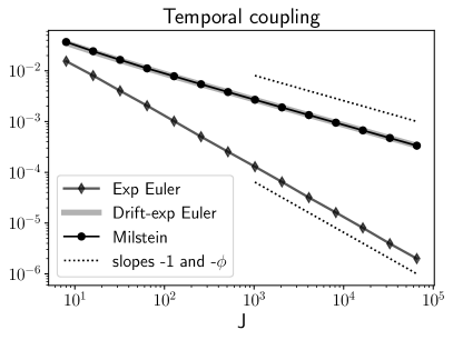
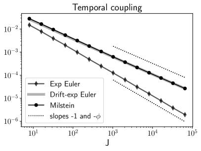
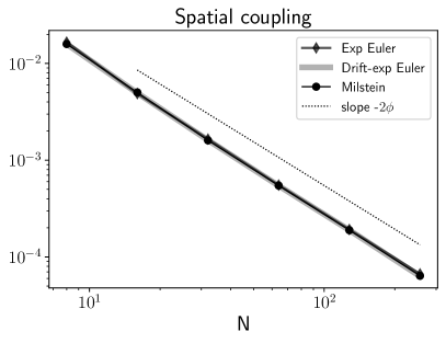
Figure 1. RMSE in time and space for the SPDE with the linear reaction term. The top row provides rates for low-regularity setting with $b=1/4$ and the bottom row provides rates for $b=1/2$.

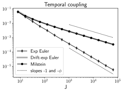
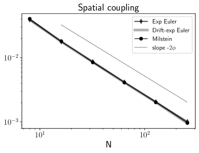
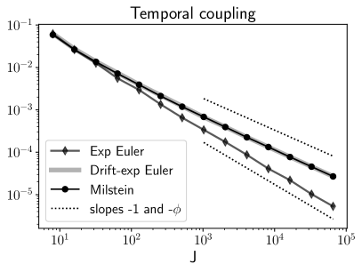
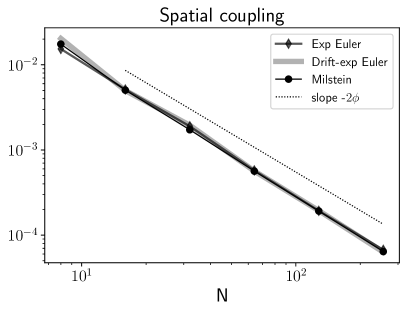
Figure 2. RMSE in time and space for the SPDE with the trigonometric reaction term. The top row provides the rates for low-regularity setting with $b=1/4$ and the bottom row provides the rates for $b=1/2$.

Since the $\beta$ in Theorem 2.7 represents the MSE, the numerical experiments indicate that $\beta=2\min(1,2\phi)=2$ for exponential Euler MLMC and $\beta=2\phi(b)=1/2+2b$ for the other two methods. We will further set $\alpha=\beta/2$ as the weak rate when implementing all MLMC methods.

4.2. Method parameters

All three methods are implemented using Theorem 2.7 with the numerical estimates of the rates $\alpha$ and $\beta$, rather than by using the rather than using the slightly more conservative rate for $\beta$ in Theorem 3.4 (ii).

4.2.1. Exponential Euler MLMC method

We use the estimated rates $\alpha=1$ and $\beta=2$ and balance error contributions in time and space by setting

$$J_{\ell}=2^{\ell+2}\quad\text{and}\quad N_{\ell}=2\times\lceil 2^{\ell/(2\phi)+1}\rceil\quad\text{and}\quad.$$

and $L=\lceil\log_{2}(1/\epsilon)/\alpha\rceil=\lceil\log_{2}(1/\epsilon)\rceil$. We set $C_{\ell}:=(\ell+1)2^{\gamma\ell}$ with $\gamma=1+1/(2\phi)$, which one may verify is consistent with $C_{\ell}\eqsim J_{\ell}N_{\ell}\log_{2}(N_{\ell})$, and we set $V_{\ell}:=2^{-2\ell}$ to determine the sequence $\{M_{\ell}\}_{\ell}$, in compliance with formula (3.15), by

(4.1) $$M_{\ell}(\epsilon)=\begin{cases}20\left\lceil 2\epsilon^{-2}\sqrt{\frac{V_{\ell}}{C_{\ell}}}\sum_{j=0}^{L}\sqrt{V_{j}C_{j}}\right\rceil&\text{if}\quad\ell=0\\[5.0pt] \;\;5\left\lceil 2\epsilon^{-2}\sqrt{\frac{V_{\ell}}{C_{\ell}}}\sum_{j=0}^{L}\sqrt{V_{j}C_{j}}\right\rceil&\text{otherwise.}\end{cases}$$

4.2.2. Drift-exponential Euler MLMC and Milstein MLMC

The numerically observed convergence rates for both of these methods are $\beta=2\phi$ and $\alpha=\phi$. For both methods, we set

$$J_{\ell}=2^{\ell+2},\quad N_{\ell}=2\times\lceil 2^{\ell/2+1}\rceil,\quad\text{and}\quad L=\left\lceil\frac{\log_{2}(1/\epsilon)}{\phi}\right\rceil-2,$$

$C_{\ell}:=(\ell+1)2^{3\ell/2}$ and $V_{\ell}:=2^{-2\phi\ell}$, we and determine the sequence $\{M_{\ell}\}_{\ell}$ by formula (4.1).

4.3. Linear reaction term

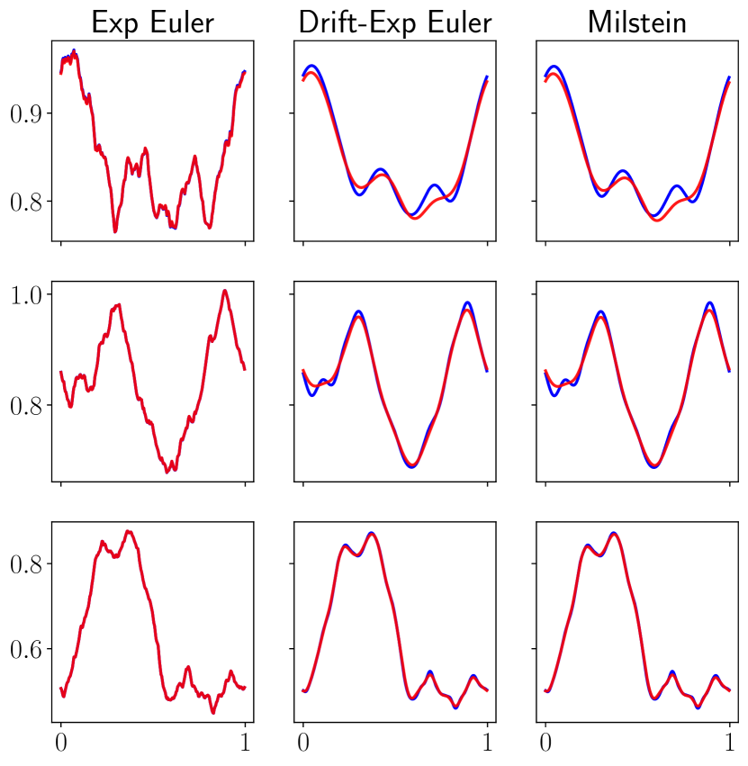
(a) $b=1/4$

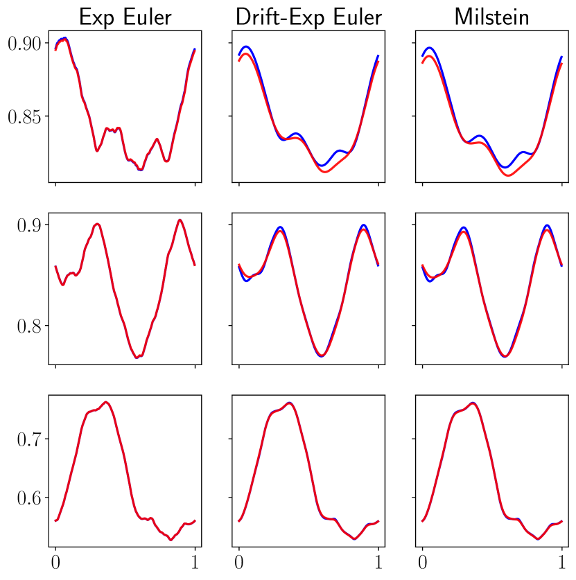
(b) $b=1/2$

Figure 3. Comparison of the couplings at the finest level (blue) and the coarsest level (red) for the SPDE with linear reaction term. The spatial resolution is fixed to $N=2^{8}$ in all simulations and the resolution in time $(J,J/2)$ is given by $J=2^{6},2^{8},$ and $2^{10}$ from top to bottom row.

We first consider the SPDE with $f(U)=U$. Figure 3 presents pairwisely coupled realizations for progressively finer resolution in time for the settings $b=1/4$ and $b=1/2$. In the low regularity setting $b=1/4$, we clearly observe that the exponential Euler method has far less smoothing of the solutions and achieves a stronger coupling than the other methods. The difference between the methods becomes less visible in the smoother setting $b=1/2$.

Figure 4 provides the approximation of $\mathbb{E}[U(T,\cdot)]$ by one simulation of each of the MLMC methods for different input $\epsilon=2^{-\ell}$ for $\ell=4,5,\ldots,9$. We observe that all methods converge to the mean with approximately the same rate for both values of $b$.

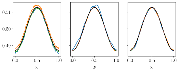
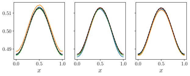
Figure 4. Approximation of $E_{\mathrm{ML}}[U(T,x)]$ for the SPDE with linear reaction term for different values of $\epsilon=2^{-4},2^{-5},\ldots,2^{-9}$ in full colored lines (blue, orange, green, red, purple, brown) and the pseudo-reference solution $\mathbb{E}[U(T,x)]$ (dashed line). From left to right, exponential Euler, drift-exponential Euler, and Milstein. Top row is for the low-regularity setting $b=1/4$ and bottom row is for $b=1/2$.

Figure 5 presents the MLMC approximation error versus tolerance and the computational cost versus tolerance for different input tolerances $\epsilon$ for one simulation. The approximation error

$$\|E_{\rm{ML}}[U(T,\cdot)](\omega;\epsilon)-\mathbb{E}{U(T,\cdot)}\|_{H}^{2}$$

is computed for one simulation of the MLMC estimator for each input of $\epsilon$, where the the pseudo-reference solution $\mathbb{E}{U(T,\cdot)}$ is obtained by solving the PDE

$$dU_{t}^{N}=(A_{N}U_{t}^{N}+f_{N}(U^{N}))dt,\qquad U_{0}^{N}=P_{N}u_{0}$$

with the exponential Euler method using the resolutions $N=2^{13}$ and $J=2^{18}$. Let us also recall that the computational cost of the MLMC methods is defined by $\sum_{\ell=0}^{L}C_{\ell}M_{\ell}$.

For $\phi=1/2-$, we observe that exponential Euler MLMC method has achieves the error $\mathcal{O}(\epsilon^{2})$ at the cost $\mathcal{O}((\log_{2}(\epsilon))^{2}\epsilon^{-2})$ while the other methods achieves similar accuracy at considerably higher cost. For $\phi=3/4-$ all three methods achieves an error $\mathcal{O}(\epsilon^{2})$ at a comparable computational cost. The observations are consistent with theory.

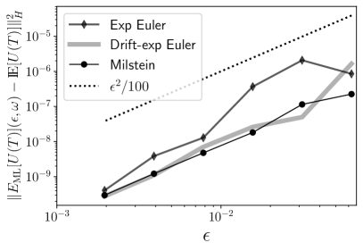
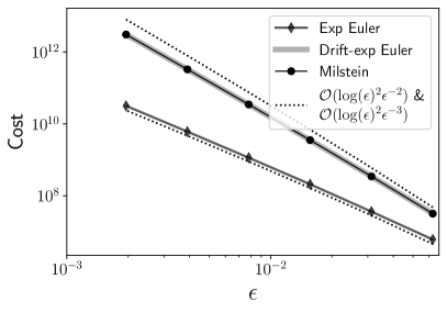
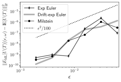
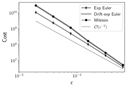
Figure 5. Top row: convergence and computational cost plots for the SPDE with $f(U)=U$ and $b=1/4$. Bottom row: similar plots for the setting with $b=1/2$.

4.4. Trigonometric reaction term

We next consider the SPDE with

$$f(U)(x)=2\big{(}\sin(2\pi U(x))+\cos(2\pi U(x))\big{)}.$$

The approximation of $\mathbb{E}[U(T,\cdot)]$ by the MLMC methods for different inputs $\epsilon=2^{-\ell}$ for $\ell=4,5,\dots,9$ is presented in Figure 6 and Figure 7 shows the MLMC approximation error versus computational cost and computational cost versus tolerance for different input tolerances $\epsilon$. For each value of $b$, the pseudo-reference solution used for evaluating the approximation error is computed by the exponential Euler MLMC method $E_{\mathrm{ML}}[U(T,\cdot)](\omega,\epsilon)\approx\mathbb{E}[U(T,\cdot)]$ with the overkilled parameter value $\epsilon=2^{-11}$. This an expensive computation using the following number of samples per level when $b=1/4$:

$$(M_{0},M_{1},M_{2},\ldots,M_{10},M_{11})=(4907168680,216868270,44268050,\ldots,355,85),$$

with $N_{\ell}=J_{\ell}=2^{\ell+2}$. We observe once again that exponential Euler MLMC outperforms the other methods in the low-regularity setting $b=1/4$ and that all methods perform similarly when $b=1/2$.

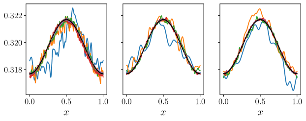
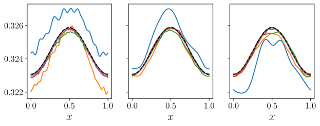
Figure 6. Approximation of $E_{\mathrm{ML}}[U(T,x)]$ for the SPDE with trigonometric reaction term for different values of $\epsilon=2^{-4},2^{-5},\ldots,2^{-9}$ in full colored lines (blue, orange, green, red, purple, brown) and the pseudo-reference solution $\mathbb{E}[U(T,x)]$ (dashed line). From left to right, exponential Euler, drift-exponential Euler, and Milstein. Top row is for the low-regularity setting $b=1/4$ and bottom row is for $b=1/2$.

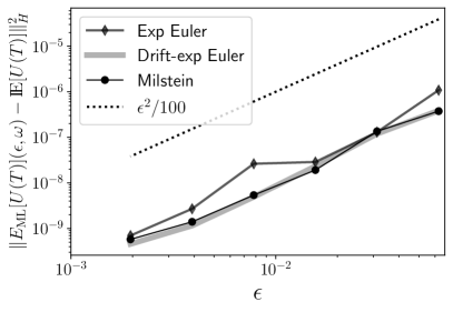
Figure 7. Top row: convergence and computational cost plots for the SPDE with $f(U)=2(\sin(2\pi U)+\cos(2\pi U))$ and $b=1/4$. Bottom row: similar plots for the setting with $b=1/2$.

5. Conclusion

Our objective in this work was to show both theoretically and experimentally that coupling approaches that exploit more information than only the driving noise $W_{t}$, such as the exponential Euler MLMC method, can result in strong coupling and improve the efficiency of weak approximations for SPDE. Our motivation in doing so, was based on the lack of literature on strong coupling for MLMC methods solving SPDE. In particular, we have derived explicit convergence rates, related to the decay of the mean squared error-to-cost rate, for the exponential Euler MLMC method and the Milstein MLMC method, cf. Theorems 3.4 and 3.6. The convergence rates for exponential Euler MLMC method is an improvement over existing MLMC methods for reaction-diffusion SPDE with additive noise. We also presented numerical experiments highlighting our derived rates and demonstrating the efficiency gains of the exponential Euler MLMC method over alternative ones. This was tested numerically on SPDE with linear and nonlinear reaction terms.

There are many possible extensions of this work. It would be interesting to understand whether strong couplings also can improve the efficiency of MLMC for other numerical solvers for SPDE, such as finite difference methods and FEM [2, 5]. This indeed is a challenging problem, due to the seemingly limitless possibilities of couplings for infinite-dimensional problems. Another direction is to develop a multi-index Monte Carlo method [18, 28] based on the pathwise correctly coupled exponential Euler method. This has the potential of further improving tractability in higher-dimensional physical space and low-regularity settings.

Appendix A Model assumptions for the exponential Euler method

Our assumptions will be similar to those in the seminal work [30] on exponential Euler integrators.

Assumption A.1.

There exists a strictly increasing sequence $(\lambda_{n})_{n=1}^{\infty}$ of positive real numbers such that $Ae_{n}=-\lambda_{n}\,e_{n}$ for $n\in{\mathbb{N}}$ and the linear operator $A:D(A)\rightarrow H$ is given as

$$Av=-\sum^{\infty}_{n=1}\lambda_{n}\langle e_{n},v\rangle\,e_{n}\quad\forall\,v\in D(A)$$

where

$$D(A)=\left\{v\in H\,\Big{|}\,\sum^{\infty}_{n=1}\lambda_{n}^{2}\,|\langle v,e_{n}\rangle|^{2}<\infty\right\}.\quad$$

We define the family of interpolation spaces of the operator $A$ for $r\geq 0$ as follows

(A.1) $$H_{r}:=D((-A)^{r})=\left\{v\in H\,\Big{|}\,\sum^{\infty}_{n=1}\lambda_{n}^{2r}\,|\langle v,e_{n}\rangle|^{2}<\infty\right\}.$$

The $Q$-Wiener process is defined by

(A.2) $$W_{t}:=\sum^{\infty}_{n=1}\sqrt{q_{n}}e_{n}w^{n}_{t},$$

where $(w^{n}_{t})_{n=1}^{\infty}$ is a sequence of independent scalar-valued Wiener processes, and the non-negative sequence $(q_{n})_{n}\subset[0,\infty)$ satisfies the following:

Assumption A.2.

There exists a constant $\phi\in(0,1)$ such that

$$\sum^{\infty}_{n=1}(\lambda_{n})^{2\phi-1}q_{n}<\infty.$$

Let $L(H_{r_{1}},H_{r_{2}})$ denote the set of bounded linear operators mapping from $H_{r_{1}}$ to $H_{r_{2}}$, and the let $L(H_{r}):=L(H_{r},H_{r})$.

Assumption A.3.

The reaction term $f:H\rightarrow H$ is twice continuously Fréchet differentiable, where its derivatives satisfy the following

$$\|f^{\prime}(x)-f^{\prime}(y)\|_{L(H)}\leq C\|x-y\|_{H},\quad\|(-A)^{-r}f^{\prime}(x)(-A)^{r}v\|_{H}\leq C\|v\|_{H},$$

for all $x,y\in H,v\in D((-A)^{\phi})$, and $r=\{0,1/2,1\}$, and

$$\|A^{-1}f^{\prime\prime}(x)(v,w)\|_{H}\leq C\|(-A)^{-1/2}v\|_{H}\|(-A)^{-1/2}w\|_{H},$$

for all $v,w\in H$, where $C>0$ is a positive constant.

Assumption A.4.

The initial value $u_{0}$ is a $D((-A)^{\phi})$-valued random variable, that satisfies

$$\mathbb{E}[\|(-A)^{\phi}u_{0}\|^{4}_{H}]<\infty,$$

for the constant $\phi>0$ in Assumption A.2.

Appendix B Model assumptions for the Milstein method

In this section, we present the assumptions for the Milstein method [31] in the setting that is relevant for this paper: when the operators $A$ and $Q$ share eigenspace and for reaction-diffusion SPDE (2.1) with additive noise.

Assumption B.1 (Drift coefficient and noise assumption).

Let Assumption A.1 hold and let Assumption A.2 hold for some $\phi\in(1/2,1)$. Let $\kappa\in[0,\phi)$ and let $f:H_{\kappa}\to H$ be a twice continuously Fréchet differentiable mapping with

$$\sup_{x\in H_{\kappa}}\max(\|f^{\prime}(x)\|_{L(H)},\,\|f^{\prime\prime}(x)\|_{L(H_{\kappa}\times H_{\kappa},H)})<\infty.$$

And for a value $\theta\in[\max(\kappa,\phi-1/2),\phi)$, it holds that

$$\mathbb{E}{\|(-A)^{\theta}u_{0}\|_{H}}<\infty.$$

Remark B.2.

Since $H_{\kappa}$ is dense in $H$, the operator $f^{\prime}(x)\in L(H_{\kappa},H)$ has a unique extension $\tilde{f}^{\prime}(x)\in L(H,H)$ and one should interpret the operator norm on the extended domain as follows:

$$\|f^{\prime}(x)\|_{L(H)}:=\sup_{v\in H_{\kappa}\setminus\{0\}}\frac{\|f^{\prime}(x)(v)\|_{H}}{\|v\|_{H}}=\|\tilde{f}^{\prime}(x)\|_{L(H)}.$$

Remark B.3.

The cryptic parameter $\theta$ is an adaptation of [31, Assumption 3] to the additive-noise setting with $B(u)=I$ and $U_{0}=Q^{1/2}(H)$. And, working with Hilbert–Schmidt operator norms, [31, equation (21)] is then fulfilled by

$$\|B(u)\|_{HS(U_{0},H_{\phi-1/2})}=\|B(u)Q^{1/2}\|_{HS(H,H_{\phi-1/2})}:=\sum_{n=1}^{\infty}q_{n}\lambda_{n}^{2\bar{\phi}-1}<\infty.$$

What we represent by $\kappa$, $\phi-1/2$ and $\theta$ is respectively denoted by $\beta$, $\delta$ and $\gamma$ in [31]. [31, equation (22)] is trivially fulfilled since $B^{\prime}(u)=0$ and choosing, in the paper’s notation, $\alpha=0$ and $\vartheta=\max(1/2-\phi,1/4)$, it follows that [31, equation (23)] holds for any $\theta\in[\max(\kappa,\phi-1/2),\phi)$, since

$$\begin{split}\|(-A)^{-\vartheta}B(u)Q^{-\alpha}\|_{HS(U_{0},H)}&=\|(-A)^{-\max(1/2-\phi,1/4)}Q^{1/2}\|_{HS(H,H)}\\ &\leq\sum_{n=1}^{\infty}\lambda_{n}^{2\phi-1}q_{n}\stackrel{{\scriptstyle Assumpt.~{}\ref{assum:noise}}}{{<}}\infty.\end{split}$$

[31, equation (23)] does indeed not depend on the value $\theta$ in the additive-noise setting, but $\theta$ does enter as a constraint on the regularity of the initial data in [31, Assumption 4]. Our lower bound $\phi>1/2$ is due to the constraint $\delta>0$ in [31, Assumption 3] and our upper bound $\kappa<\phi$ is due to the constraint $\beta<\delta+1/2$ in [31, Assumption 3].

References

- [1] M. Abdar, F. Pourpanah, S. Hussain, Dana Rezazadegan et al. A review of uncertainty quantification in deep learning: Techniques, applications and challenges. Information Fusion, 71, 243–297, 2021.
- [2] A. Abdulle, A. Barth, and C. Schwab. Multilevel Monte Carlo Methods for Stochastic Elliptic Multiscale PDEs Multiscale Model. Simul., 11(4), 1033–1070, 2013.
- [3] A. Barth and A. Lang. Multilevel Monte Carlo method with applications to stochastic partial differential equations. Int Journal of Computer Mathematics, 89(18):2479–2498, 2012.
- [4] A. Barth and A. Lang. Milstein approximation for advection-diffusion equations driven by multiplicative noncontinuous martingale noises. Applied Mathematics & Optimization, 66(3):387–413, 2012.
- [5] A. Barth, A. Lang and C. Schwab. Multilevel Monte Carlo method for parabolic stochastic partial differential equations. BIT Numerical Mathematics, 53(1):3–27, 2013.
- [6] N. K. Chada, A. Jasra and F. Yu. Multilevel ensemble Kalman–Bucy filters. arXiv preprint arXiv:2011.04342, 2020.
- [7] J. Charrier, R. Scheichl, and A.L. Teckentrup. Finite element error analysis of elliptic PDEs with random coefficients and its application to multilevel Monte Carlo methods. SIAM J. Numer. Anal., 51:322–352, 2013.
- [8] A. Chernov, H. Hoel, K. J. H. Law, F. Nobile and R. Tempone. Multilevel ensemble Kalman filtering for spatio-temporal processes. Numer. Math. 147:71-125, 2021.
- [9] G. Da Prato and J. Zabczyk. Stochastic equations in infinite dimensions. Cambridge, UK: Cambridge University Press, 1992.
- [10] T.J. Dodwell, C. Ketelsen, R. Scheichl, A.L. Teckentrup. Multilevel Markov chain Monte Carlo. SIAM Review, 61(3), 509–545, 2019.
- [11] U. Erdoan and G. J. Lord. A new class of exponential integrators for SDEs with multiplicative noise. IMA Journal of Numerical Analysis 39(2), 820–846, 2019.
- [12] T. G. Freeman. The Mathematics of Medical Imaging: A Beginner’s Guide. Springer Undergraduate Texts, 2015.
- [13] K. Fossum, T. Mannseth and A. S. Stordal. Assessment of multilevel ensemble-based data assimilation for reservoir history matching. Computational geosciences, 24, 217–239, 2020.
- [14] M. B. Giles. Multilevel Monte Carlo path simulation. Op. Res., 56 607–617, 2008.
- [15] M. B. Giles. Multilevel Monte Carlo methods. Acta Numerica, 24, 259–328, 2015.
- [16] M.B. Giles and C. Reisinger. Stochastic finite differences and multilevel Monte Carlo for a class of SPDEs in finance. SIAM J. Fin. Math., 3(1):572–592, 2012.
- [17] M. B. Giles and L. Szpruch. Antithetic multilevel monte carlo estimation for multi-dimensional sdes without lévy area simulation. The Annals of Applied Probability, 24(4):1585–1620, 2014.
- [18] A. Haji-Ali, F. Nobile and R. Tempone. Multi-index Monte Carlo: when sparsity meets sampling. Numer. Math., 132, 767–806, 2016.
- [19] H. Harbrecht, M. Peters, and M. Siebenmorgen. On multilevel quadrature for elliptic stochastic partial differential equations. In J. Garcke and M. Griebel, editors, Sparse grids and applications, volume 88 of Lecture Notes in Computational Science and Engineering, 161–179. Springer, Berlin-Heidelberg, 2013.
- [20] E. Hausenblas. Numerical analysis of semilinear stochastic evolution equations in Banach spaces. Journal of Computational and Applied Mathematics, 147, 485–516, 2002.
- [21] E. Hausenblas. Approximation for semilinear stochastic evolution qquations. Potential Analysis, 18, 141–186, 2003.
- [22] S. Heinrich. Multilevel Monte Carlo methods. In Large-Scale Scientific Computing, (eds. S. Margenov, J. Wasniewski & P. Yalamov), Springer: Berlin, 2011.
- [23] M. Hochbruck and A. Ostermann. Exponential integrators. Acta Numerica, 209–286, 2010.
- [24] H. Hoel, K. J. H. Law and R. Tempone. Multilevel ensemble Kalman filtering. SIAM J. Numer. Anal., 54(3), 1813–1839, 2016.
- [25] H. Hoel, G. Shaimerdenova, and R. Tempone. Multilevel ensemble kalman filtering based on a sample average of independent enkf estimators. Foundations of Data Science, 2(4):351–390, 2020.
- [26] A. Jasra, K. Kamatani, K. J. H. Law and Y. Zhou. Multilevel particle filters. SIAM J. Numer. Anal., 55(6), 3068–3096, 2017.
- [27] A. Jasra, K. Kamatani, K. J. H. Law and Y. Zhou. A multi-index Markov chain Monte Carlo method. Int’l J. Uncer. Quant., 8(1), 2018.
- [28] A. Jasra, K. J. H. Law and Y. Xu. Multi-Index sequential Monte Carlo methods for partially observed stochastic partial differential equations. Int’l J. Uncer. Quant. , 11, 1–25, 2021.
- [29] A. Jentzen. Stochastic partial differential equations: Analysis and numerical approximations. ETH Zurich Lecture Notes, 2016.
- [30] A. Jentzen and P. E. Kloeden. Overcoming the order barrier in the numerical approximation of stochastic partial differential equations with additive space-time noise. Proc. R. Soc. A Math. Phys. Eng. Sci. 465, 649–667, 2009.
- [31] A. Jentzen and M. Röckner. A Milstein scheme for SPDEs. Found. Comput. Math., 15(2):313–362, 2015.
- [32] P. E. Kloeden and E. Platen. Numerical Solution of Stochastic Differential Equations. Applications of Mathematics (New York) 23. Springer, Berlin, 1992.
- [33] P. E. Kloeden, G. J Lord, A. Neuenkirch, and T. Shardlow. The exponential integrator scheme for stochastic partial differential equations: Pathwise error bounds. Journal of Computational and Applied Mathematics, 235(5):1245–1260, 2011.
- [34] A. Lang and A. Petersson. Monte Carlo versus multilevel Monte Carlo in weak error simulations of SPDE approximations. Mathematics and Computers in Simulation,143: 99–113, 2018.
- [35] G. J. Lord, C.E. Powell and T. Shardlow. An Introduction to Computational Stochastic PDEs, Cambridge Texts in Applied Mathematics, 2014.
- [36] G. J. Lord and A. Tambue. Stochastic exponential integrators for the finite element discretization of SPDEs for multiplicative and additive noise. IMA Journal of Numerical Analysis 33(2), 515–543, 2013.
- [37] A. Majda and X. Wang. Non-linear Dynamics and Statistical Theories for Basic Geophysical Flows, Cambridge University Press, 2006.
- [38] E.H. Mller, R. Scheichl and T. Shardlow. Improving multilevel Monte Carlo for stochastic differential equations with application to the Langevin equation. Royal Society Proceedings A, 2015
- [39] C. Robert and G. Casella. Monte Carlo statistical methods, Springer Science & Business Media, 2013.
- [40] T. J. Sullivan. Introduction to Uncertainty Quantification. Texts in Applied Mathematics 63, Springer, 2014.
- [41] R. C. Smith. Uncertainty Quantification: Theory, Implementation, and Applications. SIAM textbooks, 2013.
- [42] D. Xiu. Numerical Methods for Stochastic Computations: A Spectral Method Approach. Princeton University Press, Princeton, NJ, 2010.
- [43] Z. Zhang and G. E. Karniadakis. Numerical Methods for Stochastic Partial Differential Equations with White Noise. Applied Mathematical Sciences, Springer, 2017.