On the importance of wave planet interactions for the migration of two super-Earths embedded in a protoplanetary disk

Abstract

We investigate a repulsion mechanism between two low-mass planets migrating in a protoplanetary disk, for which the relative migration switches from convergent to divergent. This mechanism invokes density waves emitted by one planet transferring angular momentum to the coorbital region of the other and then directly to it through the horseshoe drag. We formulate simple analytical estimates, which indicate when the repulsion mechanism is effective. One condition for a planet to be repelled is that it forms a partial gap in the disk and another is that this should contain enough material to support angular momentum exchange with it. Using two-dimensional hydrodynamical simulations we obtain divergent migration of two super-Earths embedded in a protoplanetary disk because of repulsion between them and verify these conditions. To investigate the importance of resonant interaction we study the migration of planet pairs near first-order commensurabilities. It appears that proximity to resonance is significant but not essential. In this context we find repulsion still occurs when the gravitational interaction between the planets is removed sugesting the importance of angular momentum transfer through waves excited by another planet. This may occur through the scattering of coorbital material (the horseshoe drag), or material orbiting close by. Our results indicate that if conditions favor the repulsion between two planets described above, we expect to observe planet pairs with their period ratios greater, often only slightly greater, than resonant values or possibly rarity of commensurability.

1 Introduction

The early stages of the evolution of multi-planet systems that occurs after their formation, when gaseous protoplanetary disks are still present, have been studied in many works (e.g. Nelson & Papaloizou, 2002; Kley et al., 2004; Papaloizou & Szuszkiewicz, 2005; Kley & Nelson, 2012). One of the important outcomes of this evolutionary phase is an inevitable process of planetary migration taking place in a gaseous environment. It is expected that when there is convergent migration of two planets they can be trapped in mean-motion resonances (MMRs). The frequency of the occurrence of MMRs is therefore a robust feature to be tested against predictions based on the results of numerical simulations. The observational data indicates that planet pairs with period ratios close to commensurability are not as common as simulations, that adopt simple prescriptions for migration rates, indicate. Moreover, the multiple systems observed by the Kepler mission are such that the planet pairs near resonances tend to have period ratios slightly larger than those required for strict commensurability, especially in the case of the 3:2 and 2:1 resonances (e.g Lissauer et al., 2011; Fabrycky et al., 2014; Steffen & Hwang, 2015). This has been found for both pairs of giant planets and systems composed of two low-mass planets.

One example of these is the Kepler-59 system, which contains two planets with masses of $5M_{\oplus}$ and $4.6M_{\oplus}$ being the inner and outer planet respectively. The orbital period ratio is 1.5141 (Saad-Olivera et al., 2020). Another example is the Kepler-128 system in which the inner and outer planets have masses equal to $0.77M_{\oplus}$ and $0.9M_{\oplus}$, respectively and their period ratio is 1.5112 (Hadden & Lithwick, 2016). In both planetary systems, the orbital period ratio of two planets is slightly larger than $3/2.$

Furthermore, several two-planet systems with planet masses in the super-Earth range possess period ratios close to other first-order resonances. The two low-mass planets in the Kepler-177 system are near the 4:3 resonance (Hadden & Lithwick, 2017; Vissapragada et al., 2020). In the Kepler-307 system, two super-Earths are close to 5:4 resonance (Jontof-Hutter et al., 2016) and in Kepler-36 the period ratio is close to 7:6 (Carter et al., 2012; Vissapragada et al., 2020). It is worth mentioning that in the case of the Kepler-59 and Kepler-307 systems, the outer planet is less massive than the inner one. Detailed information about the planetary systems mentioned above is given in Table 1.

Table 1: Two-planet systems with the period ratios near the first-order resonances

System	Planet pair	Period (days)	Mass ($M_{\star}$)	Resonance	Deviation of period ratio	Reference
				$p+1:p$	from $(p+1)/p$
Kepler-59	Kepler-59b	11.8715	$1.10\times 10^{-5}$	3:2	0.0141	Saad-Olivera et al. (2020)
	Kepler-59c	17.9742	$1.02\times 10^{-5}$
Kepler-128	Kepler-128b	15.090	$2.12\times 10^{-6}$	3:2	0.0112	Hadden & Lithwick (2016)
	Kepler-128c	22.804	$2.48\times 10^{-6}$
Kepler-177	Kepler-177b	35.860	$1.90\times 10^{-5}$	4:3	0.0445	Vissapragada et al. (2020)
	Kepler-177c	49.409	$4.79\times 10^{-5}$
Kepler-307	Kepler-307b	10.4208	$2.46\times 10^{-5}$	5:4	0.0045	Jontof-Hutter et al. (2016)
	Kepler-307c	13.0729	$1.20\times 10^{-5}$
Kepler-36	Kepler-36b	13.8683	$1.11\times 10^{-5}$	7:6	0.0028	Vissapragada et al. (2020)
	Kepler-36c	16.2187	$2.07\times 10^{-5}$

A better understanding of the distribution of the observed period ratios is a key ingredient in any model of the formation of compact planetary systems. Many mechanisms have been put forward to explain the reasons for the departure from strict mean-motion resonance that would be expected as a result of migration in the protoplanetary disk. In the case of planets orbiting close to their parent stars, a mechanism driven by dissipation induced by tides raised on the planets by the central star can be particularly effective (Papaloizou & Terquem, 2010; Papaloizou, 2011; Lithwick & Wu, 2012; Batygin & Morbidelli, 2013; Lee et al., 2013; Delisle & Laskar, 2014).

A mechanism to account for the departure from resonance or more generally for the forestallment of the attainment of commensurability, regardless of the distance from which a planet pair orbits its parent star, has been identified. This considers the effects of the density waves excited by one of the planets on the other one. In particular the transfer of the angular momentum carried by the waves to the other planet can lead to divergent migration, thus preventing the planets from being closely locked into any MMR.

In Podlewska-Gaca et al. (2012), these effects were investigated in a system containing an inner giant planet (a source of the outward propagating density waves) and an outer super-Earth, using both global two-dimensional hydrodynamical calculations and local shearing box simulations. They showed that the inward migration of the super-Earth could be stopped or even reversed due to the angular momentum transfer by the outgoing density waves.

Similar interactions between the planets and the disk were studied for planet pairs consisting of two Saturn-like planets as well as two less massive Uranus-like ones in Baruteau & Papaloizou (2013). They found that the disk-driven repulsion, described above, that leads to the divergent migration of the planets, is particularly efficient when at least one of the planets opens a partial gap in the disk.

The migration of planets, which are able to form a partial gap has attracted a lot of attention recently (e.g. Duffell et al., 2014; Dürmann & Kley, 2015, 2017; Kanagawa et al., 2018). The way in which such planets migrate is crucial for answering questions about several aspects of planetary system formation and early evolution, and in particular about the possibility of forming mean-motion resonances. This issue has been recently investigated by Kanagawa & Szuszkiewicz (2020).

The aim of this paper is to extend previous studies to pairs of low-mass planets with masses in the super-Earth range embedded in a disk in which they are capable of opening a partial gap in which they orbit.

The main focus is put on the repulsion mechanism responsible for the divergent migration that prevents capture into a strict commensurability. We check that the angular momentum flow between the planets is consistent with theoretical expectation for the density waves they produce and that the angular momentum flow resulting from the density waves emitted by one into the horseshoe region of the other can account for the torque required to produce the switch from convergent to divergent migration. As a result, we are able to identify the nature of the repulsion between low-mass planets migrating in the protoplanetary disk and demonstrate that it can occur for super-Earths with masses below 10 Earth masses. Finally, we provide simple analytical estimates, which indicate when this repulsion is effective. The observational consequences of the repulsion mechanism found in this paper might be important but to come up with more quantitative picture requires further studies.

The plan of this paper is as follows. In Section 2 we describe the disk and planet parameters adopted in our investigations. In Section 3 we describe two-dimensional hydrodynamical simulations of two super-Earths that after an initial period of convergent migration towards the vicinity of the 3:2 MMR ultimately undergo divergent migration.

In order to separate genuine single planet evolution from the effects caused by the presence of a second planet, in Section 4 we analyse the migration of a single super-Earth corresponding to the outer component of the system considered in Section 3. Because this planet opens a partial gap in the disk, standard type I migration does not apply. Accordingly we provide simple fits to our numerical data for different surface density profiles, using these to quantify deviations seen in the two planet simulations in Section 5. In Section 6 we describe a simple model for how density waves emitted by one planet being absorbed in the horseshoe region of the other can lead to planet-planet repulsion, giving criteria for the mechanism to be effective. We go on to verify these for systems having a range of mass ratios in Section 7 and study the dependence of the initial rate of convergent migration on the disk surface density and planet mass ratios in Section 8.

The consistency of the angular momentum flow associated with density waves with the torque necessary to provide the repulsion between planets is investigated in Section 9. We then establish the robustness of our results to changes of the surface density profile, the adopted equation of state, and the effect of neglecting the disk self-gravity in Sections  10 - 11. In order to consider protoplanetary disks with significantly smaller surface densities that may occur during the dispersal process possibly produced by photoevaporation, we examine the repulsion mechanism in disks with significantly reduced surface densities in Section 12 and finally we demonstrate the effectiveness of the repulsion mechanism for the super-Earths migrating in a viscous disk in which the temperature is determined by the balance between local heating and cooling and which supports a constant angular momentum flux in Section 13. This situation may arise when the inner disk is disrupted by the magnetosphere of the central star (eg. Clarke & Armitage, 1996). Finally, we summarise our results and conclude in Section 14.

2 Disk model and numerical setup

We consider a system of two planets with masses $m_{1}$ (inner planet) and $m_{2}$ (outer planet), orbiting a central star of mass $M_{\star}$, while being embedded in a protoplanetary disk. We will find it convenient to make use of the planet-to-star mass ratios $q_{i}=m_{i}/M_{\star}$ with $i=1$ denoting the inner planet and $i=2$ denoting the outer one. A two-dimensional disk model is adopted together with a cylindrical polar coordinate system ($r,\phi$, z) with origin located at the central star which is regarded as a point mass. We start our investigations from the simple disk model described by the continuity equation and the equation of motion in the form:

$$\frac{\partial\Sigma}{\partial t}=-\nabla\cdot(\Sigma\bf{v})$$ (1)

and

$$\frac{\partial\bf{v}}{\partial t}+{\bf{v}}\cdot\nabla{\bf{v}}=-\frac{1}{\Sigma}\nabla P-\nabla\Phi+{\bf{f}}_{\nu}$$ (2)

where $\Sigma$ and ${\bf v}$ denote the surface density of the disk and the velocity, while $\Phi$ is the gravitational potential and ${\bf f}_{\nu}$ is the viscous force per unit mass. We adopt a locally isothermal equation of state, where the vertically integrated pressure can be expressed as $P=\Sigma c_{s}^{2}$, with the sound speed related to the pressure scale height of the disk, $H$, through $c_{s}=(H/r)(GM_{\star}/r)^{1/2}$. Here $G$ is the gravitational constant. The aspect ratio of the disk, $h=H/r$, is assumed to be constant in the simulation, which leads to $c_{s}^{2}\propto r^{-\beta}$ with $\beta=1.$ Thus, the power-law index of the radial temperature profile is equal to $-1$. We go on to perform a calculation with an adiabatic equation of state where $P$ is given by $P=(\gamma-1)e\Sigma$. Here $\gamma$ is the adiabatic index and $e$ is the specific internal energy in Section 11.1. The self-gravity of the disk is neglected in our simulations. The effect of this assumption has been investigated and discussed in Section 11.2. Finally, we adopt a viscous disk model, in which the temperature is determined by the balance between local heating and cooling and which supports a constant angular momentum flux. The formulation of this model is given in Section 13.

The system of units adopted in this paper is as follows: The unit of mass is the mass of the central star $M_{\star}$. The unit of length is the initial orbital radius of the inner planet $r_{1}$. The time unit is the initial orbital period of the inner planet $P_{1}$. To fix on particular parameters we can think of initiating the inner planet in a circular orbit at $r_{1}=1\rm~{}au$ and take $M_{\star}$ to be the mass of the Sun. Then, the time unit is $1\rm~{}yr$. However, we note that the results can be scaled to apply to other values of $r_{1}$ and $M_{\star}.$

In our simulations the initial orbital eccentricities of both planets are set to be zero. The initial orbital radii of the two planets in the disk are $r_{1}=1$ for the inner planet and $r_{2}=1.48$ for the outer one. The masses of the inner and outer planets are in the super-Earth mass range.

The initial surface density profile $\Sigma(r)$, adopted in the majority of our simulations that incorporate a central disk cavity is given by

$$\Sigma(r) =1.25\Sigma_{0}r-0.25\Sigma_{0}\hskip 15.649pt{\rm for} r_{\rm min}<r<1,$$

$$\Sigma(r) =\Sigma_{0}r^{-\alpha}\hskip 56.9055pt\ \ {\rm for} 1\leq r<r_{\rm max},$$ (3)

where $\Sigma_{0}$ is a scaling parameter while $r_{\rm min}$ and $r_{\rm max}$ are the inner and outer boundaries of the computational domain, respectively. In this work, if not stated differently, we take $\Sigma_{0}=6\times 10^{-5}$ in units of $M_{\star}/r_{1}^{2}$ and $\alpha=1/2$. We remark that $\pi\Sigma_{0}$ is approximately the disk mass in units of $M_{\star}$ within $r_{1}.$ In this case for $M_{\star}=1M_{\odot},$ this is $0.19$ Jupiter masses. For $r_{1}=1$ au this is about five times smaller than expected for the minimum mass solar nebula. This particular surface density profile is found to guarantee the convergent migration of super-Earths in the early stages of their evolution. The surface density of the inner part of the disk decreases sharply on moving inwards resulting in the formation of a trap where the migration of an incoming low mass planet is halted (Masset et al., 2006). In this way, the migration of the inner planet may be stopped while the outer planet being external to the trap continues to migrate inwards. Thus ensures that in the early stages of the simulations the planets will undergo convergent migration.

The governing hydrodynamical equations are solved by using the numerical code FARGO3D (Benitez-Llambay & Masset, 2016). A constant kinematic viscosity, $\nu$, is adopted to model the transport presumed to result from turbulence. The computational domain in the radial direction extends from $r_{\rm min}=0.2$ to $r_{\rm max}=2.6$ and covers the whole $2\pi$ domain in azimuth. The resolution in the calculations is 900 equal cells forming a staggered grid in the radial direction and 1800 equal cells in the azimuthal direction. We found it advantageous to adopt a rotating frame that corotates with the Keplerian angular velocity at the initial location of the inner planet. The standard outflow boundary conditions are applied at the disk boundaries and wave killing-zones (de Val-Borro et al., 2006) operate in the domains $[0.2,0.32]$ and $[2.36,2.6]$ which are connected to the inner and outer boundaries of the computational domain, respectively.

The gravitational potential at any point, $\Phi,$ is the sum of the potential due to the central star and the potential due to the planets, $\Phi_{i},i=1,2.$ When working out the force per unit mass on any planet, there is in addition to the contribution due to direct gravitational interaction, an indirect term that arises on account of the acceleration of the origin of the coordinate system that is constrained to be centred on the star. The softened potential due to a planet with mass $m_{i}$ has the form:

$$\Phi_{i}=-\frac{Gm_{i}}{\sqrt{r^{2}-2rr_{i}\cos(\phi-\phi_{i})+r_{i}^{2}+b^{2}r_{i}^{2}}}$$ (4)

where $m_{i}$ is the mass of the planet, $(r_{i},\phi_{i})$ are the cylindrical coordinates of the planet, and $b$ is the softening parameter. The latter is adopted to take account of the fact that the disk material is distributed over the vertical extent of the disk in an approximate manner. The value of $b$ is taken to be equal to $0.6h$.

In all simulations in which the equation of state is locally isothermal the disk aspect ratio is adopted to be $h=0.02$ and the viscosity is taken as $\nu=1.2\times 10^{-6}$ in units of $r_{1}^{2}(GM_{\star}/r_{1}^{3})^{1/2}$. These correspond to the expected aspect ratio at $0.1\rm~{}au$ given $h=0.05$ at $5\rm~{}au$ and the scaling $h\propto r^{1/4}$ corresponding to the source of heating being radiation from the central star, and a Shakura & Sunyaev (1973) $\alpha$-viscosity parameter equal to $0.003.$

For the disk parameters taken in our study, the two super-Earths are such that the parameters $q_{i}^{1/3}/h,$ and $q_{i}/(40\nu)$ which respectively measure the degree of nonlinearity and the ratio of tidal to viscous torques are respectively $\sim 1$ and $\sim 0.25.$ Thus the planets are expected to open a partial gap in the disk around their orbits (see Lin & Papaloizou, 1993; Korycansky & Papaloizou, 1996; Crida et al., 2006).

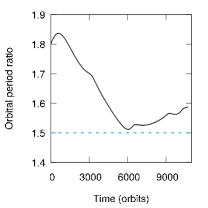
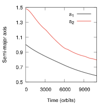
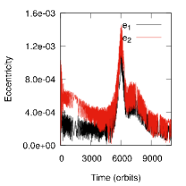
Figure 1: The results of the hydrodynamical simulation of two super-Earths with $q_{1}=1.3\times 10^{-5}$ and $q_{2}=1.185\times 10^{-5}$ migrating in a protoplanetary disk with $\Sigma=8\times 10^{-5}r^{-1/2}$, $h=0.02$ and $\nu=1.2\times 10^{-6}$. The evolution of the orbital period ratio, the semi-major axes, the eccentricities and the resonance angles are shown in the panels from left to right. The horizontal dashed blue line in the first panel indicates the position of the 3:2 commensurability.

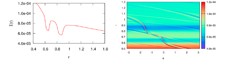
Figure 2: The results of the hydrodynamical simulation of two super-Earths with $q_{1}=1.3\times 10^{-5}$ and $q_{2}=1.185\times 10^{-5}$ migrating in a protoplanetary disk with $\Sigma=8\times 10^{-5}r^{-1/2}$, $h=0.02$ and $\nu=1.2\times 10^{-6}$. The azimuthally averaged surface density profile and a contour plot of the surface density of the disk in the vicinity of two planets at $t\sim 8560$ orbits are shown.

3 The divergent migration of two super-Earths in a protoplanetary disk following a period of convergent migration

In this Section we describe the evolution of two super-Earths evolving dynamically in a gaseous protoplanetary disk in the vicinity of the 3:2 mean-motion resonance using full two-dimensional hydrodynamic simulations. The aim of the calculations is to verify if the system of two super-Earths having undergone a period of convergent migration can see this reversed and subsequently undergo divergent migration. This phenomenon is similar to that observed in systems containing a Jupiter mass planet and a super-Earth (Podlewska-Gaca et al., 2012), two gaseous giants with the masses similar to that of Saturn, and two ice giants with masses similar to that of Uranus (Baruteau & Papaloizou, 2013).

The initiation of the migrating planets close to a first-order commensurability gives us an opportunity to investigate the role, if any, of the mean-motion resonance in determining the orbital evolution of two super-Earths. We consider two low-mass planets with $q_{1}=1.3\times 10^{-5}$ and $q_{2}=1.185\times 10^{-5}$. Both planets will open a partial gap in the disk with aspect ratio $h=0.02$ and viscosity $\nu=1.2\times 10^{-6}$ that we consider here. This is our flagship case and it will serve as a reference for numerous simulations presented in the present paper.

At the beginning of the simulation the planets are located in circular orbits with $r_{2}/r_{1}=1.48.$ The initial orbital period ratio being $1.8$ exceeds 3:2 (see Figure 1). For this simulation the initial surface density is taken to be $\Sigma=\Sigma_{0}r^{-\alpha}$, where $\Sigma_{0}=8\times 10^{-5}$ and $\alpha=0.5$. In this case we did not adopt the surface density profile given by Equation (2) as it is not required to establish initially convergent migration of the planets.

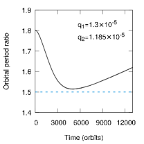
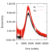
Figure 3: The results of the hydrodynamical simulation of the orbital evolution of the two super-Earths with $q_{1}=1.3\times 10^{-5}$ and $q_{2}=1.185\times 10^{-5}$ migrating in a protoplanetary disk with the initial surface density given by Equation (2), $\Sigma_{0}=6\times 10^{-5}$, $h=0.02$ and $\nu=1.2\times 10^{-6}$. The evolution of the planets’ orbital period ratio, the semi-major axes, the eccentricities and the resonance angles are shown in the panels from left to right. The horizontal dashed blue line in the first panel indicates the position of the 3:2 commensurability.

The results of the simulation for the evolution of the orbital period ratio, the semi-major axes, the eccentricities $e_{1}$, $e_{2}$ and the resonance angles associated with the 3:2 mean-motion resonance, are shown in Figure 1. As can be seen from this figure, both planets migrate inwards for the duration of the calculation. The migration rate of the outer planet slows down noticeably at times $t\sim 3000$ and $t\sim 6000$ orbital periods measured at the initial location of the inner planet, hereafter simply denoted as orbits.

The first slowdown in the migration rate of the outer planet at around $t\sim 3000$ orbits can be identified with the passage of the two planets through the 5:3 mean-motion resonance, while the second at $t\sim 6000$ orbits with the vicinity of the 3:2 commensurability. The characteristic rise in both planet eccentricities close to the 3:2 resonance is clearly visible. The eccentricities are excited by a factor of ${\sim}$ three and that of the inner planet reaches a value of 0.0011. The temporary capture into the 3:2 resonance is also illustrated by the evolution of the resonance angles, defined in Figure 1, which are seen to enter into libration.

Beyond $t\sim 6000$ orbits, the migration has changed from convergent to divergent. The orbital period ratio is increasing and the eccentricities are decreasing. At $t\sim 6500$ orbits the migration reverts to being weakly convergent and the eccentricities are increasing again. This behaviour does not last long and at $t\sim 7500$ orbits the relative migration changes back to being divergent.

Another short episode of convergent migration takes place at around $t\sim 9000$ orbits, but apart from these two brief periods of convergent migration, the overall migration is obviously divergent from $t\sim 6000$ orbits till the end of the calculation.

In Figure 2 we illustrate the azimuthally averaged surface density profile at $t\sim 8560$ orbits. A contour plot of the disk surface density in the vicinity of the two planets is shown in the right panel. Both planets develop a partial gap in the disk. As illustrated in the left panel these gaps are well separated.

3.1 Migration in a disk with an inner protoplanet trap

The detailed analysis of the mechanism, responsible for the observed evolution, necessitates studies of a range of masses of the inner planet. For this purpose, the particular surface density profile given by Equation (2) with $\Sigma_{0}=6\times 10^{-5}$ is adopted to guarantee the convergent migration of the super-Earths in the early stages of the evolution. For consistency with these calculations we have rerun the simulation already described above starting with this surface density profile. The results are shown in Figure 3. They are qualitatively very similar to those shown in Figure 1. We illustrate this fact in Figure 4 where the evolution of the orbital period ratio for both simulations are shown for comparison in the same panel.

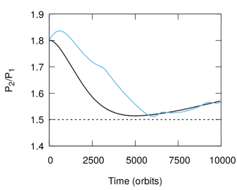
Figure 4: The comparison between the period ratio evolution for two super-Earths with $q_{1}=1.3\times 10^{-5}$ and $q_{2}=1.185\times 10^{-5}$ migrating in protoplanetary disks with initial surface density given by Equation (2) with $\Sigma_{0}=6\times 10^{-5}$ (black line), and with initial surface density profile given by $\Sigma=8\times 10^{-5}r^{-1/2}$ (light blue). The disk aspect ratio $h=0.02$ and viscosity $\nu=1.2\times 10^{-6}$ are the same in both runs.

The planets undergo the convergent migration at the beginning of the simulation. The outer planet migrates inwards and the inner one almost does not migrate as a result of the initial surface density profile adopted in this simulation decreasing rapidly inwards. A consequence of this is that the relative migration is initially faster in this case and there is no sign of passage through the 5:3 resonance on the way to the 3:2 commensurability.

At $t\sim 4000$ orbits, the system is in the vicinity of the 3:2 resonance. The eccentricities of two planets are increasing while both resonance angles associated with the 3:2 MMR begin to librate. As the resonance is entered, the inner planet is released from the trap and begins to migrate slowly inwards. The two planets then migrate inwards together briefly maintaining an approximately fixed period ratio under the effect of the mean-motion resonance.

At $t\sim 5000$ orbits, the planets are very close to the 3:2 MMR. The eccentricities have attained maximum values $e_{1}\sim 8.5\times 10^{-4}$ and $e_{2}\sim 1.0\times 10^{-3}$. Subsequently, the convergent migration of two planets changes to being divergent. The orbital period ratio of the system increases and the planets separate from the 3:2 MMR. The eccentricities subsequently decrease and the libration amplitudes of the resonance angles increase. The inward migration rate of the outer planet slows down and when $t\sim 8000$ orbits is reached the migration of the outer planet reverses and it starts to migrate outwards. The migration rate of the inner planet also decreases becoming almost zero at the end of the calculation.

In order to obtain an understanding of the mechanisms responsible for the results of the above simulations, in particular the switch from convergent to divergent migration and the increasing separation from resonance, we study in detail the way an isolated super-Earth migrates in disks with varying background surface density profiles in which it creates a partial gap. This enables us to separate features that can be understood in terms of isolated planets from those that are related to influences of one planet on another.

4 The migration of an isolated super-Earth that is capable of forming a partial gap

In this Section we provide a close look at the evolution of the outer super-Earth ($q=1.185\times 10^{-5}$) without the presence of the inner planet in the disk. We consider a range of background surface density profiles.

4.1 Setup of the simulations

In these calculations the outer super-Earth is placed on the same initial circular orbit in the disk as in the two-planet case. We adopt the same initial disk properties as in the case of two planet simulations, starting with the surface density profile given by Equation (2). Thus $h=0.02$, $\nu=1.2\times 10^{-6}$, $\Sigma_{0}=6\times 10^{-5}$ and for the first simulation $\alpha=0.5.$

In addition to the run with $\alpha=0.5$, we perform two additional runs, the first with $\alpha=-0.067$ corresponding to an almost flat surface density profile, and the second with $\alpha=-0.3$ corresponding to a profile that increases outwards. All other disk parameters are unchanged. The choices of $\alpha$ are based entirely on the form of the evolving surface density profile observed in the vicinity of the outer planet in the calculation performed with two planets. In that calculation the slope of the surface density distribution at the outer planet location evolves in time, starting from the initial slope with $\alpha=0.5$, passing through the flat profile ($\alpha=0.0$) and ending with the positive slope ($\alpha\approx-0.3$).

4.2 Relevant length scales

Before describing the migration of the single planet in the disk we first discuss the relevant length scales in the calculations. The Hill radius, $r_{H}=(q/3)^{1/3}r_{p}=0.0158r_{p}$, where $r_{p}$ is the radius at which the planet is located, is comparable to the local thickness of the disk, which is, as we have already stated, $0.02r_{p}.$ The half-width of the horseshoe region, $x_{s}/r_{p}$, can be determined from the topology of the gas flow in the vicinity of the planetary orbit. It has been determined by Paardekooper & Papaloizou (2009) to be $x_{s}\sim r_{p}\sqrt{q/h}.$ This value can be understood in the following way. The streamline which passes through the location of the planet (possible as the potential is softened) starts at large azimuthal distance with radial separation $x_{s}.$ The speed relative to the planet is $3\Omega_{p}x_{s}/2,$ where $\Omega_{p}$ is the Keplerian angular velocity at the planet’s location. In reaching the planet the kinetic energy per unit mass of material on this streamline is changed by $\sim\Omega_{p}^{2}x_{s}^{2}.$ This must be comparable to the change in planet potential $GqM_{\star}/(r_{p}b).$ Note the use of the softening length here as we anticipate this will exceed $x_{s}$ for small $q.$ Hence we deduce $x_{s}\sim r_{p}\sqrt{q/b}.$ Note that $b$ is comparable to $h$ here and Paardekooper & Papaloizou (2009) found that in the limit $b\rightarrow 0,$ the effect of back pressure is to limit the magnitude of the potential in a way that effectively replaces $b$ by $h.$ Hence $x_{s}\sim r_{p}\sqrt{q/h}.$

We show a contour plot of the surface density of the disk for the calculation with $\alpha=0.5$ in the vicinity of the planet together with the gas flow velocity field at $t=1000$ orbits in Figure 5.

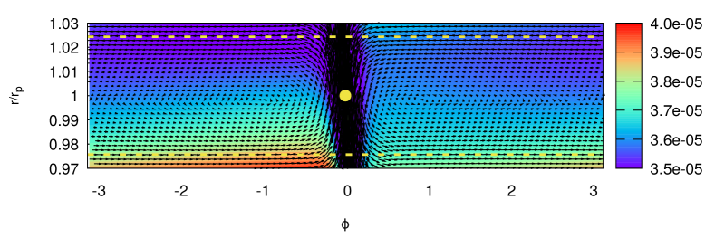
Figure 5: A snapshot of the surface density and the gas velocity field in the vicinity of the planet at $t=1000$ orbits in the simulation with $\alpha=0.5$. The yellow solid circle indicates the position of the planet and the dashed horizontal yellow lines show the position of a putative separatrix at $r=r_{p}\pm r_{p}\sqrt{q/h}$.

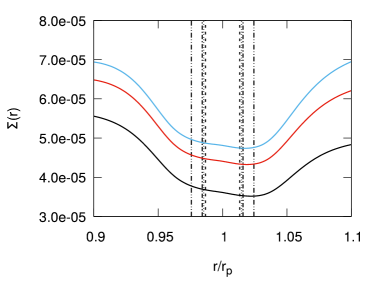
Figure 6: The distances from the orbit of the planet of the radial locations determining the characteristic scales in the problem, listed starting from the closest to the planet and proceeding to the most distant, ($(2/3)H$ - dashed, $l_{sh}$ - dotted, $r_{H}$ - dash-dotted and $x_{s}$ - dash double-dotted lines). Also plotted are the surface density profiles of the disk in the vicinity of the planet after $t=1000$ orbits when it had reached $r_{p}\sim 1.413$ in the simulations with different values of $\alpha$ (0.5 - black, $-0.067$ - red and $-0.3$ - blue lines).

Following the trend indicated by arrows directed along the gas velocity vectors in the disk, it can be concluded that the horseshoe region extends approximately from $r=r_{p}-r_{p}\sqrt{q/h}$ to $r_{p}+r_{p}\sqrt{q/h}$, as indicated by the dashed lines in the figure. It can be inferred that a streamline that is close to one of these lines will pass through the location of the planet, hence the half-width of the region $\sim x_{s}$ is such that

$$\frac{x_{s}}{r_{p}}=\sqrt{\frac{q}{h}}=0.0243.$$ (5)

This is in a good agreement with previous numerical studies as for example in Paardekooper & Papaloizou (2009). In our other two simulations the width of the horseshoe region is very similar.

Another potentially relevant scale is the non-linear shocking length $l_{sh}.$ This is the distance from the planet at which the density wave produced by the planet becomes nonlinear and shocks, $q,$ being assumed to be small enough that the wave is linear close to the planet. It is defined through (Dong et al., 2011)

$$\frac{l_{sh}}{r_{p}}\approx 0.8\left(\frac{\gamma+1}{12/5}\frac{m_{p}}{M_{th}}\right)^{-2/5}h$$ (6)

with $M_{th}=c_{s}^{3}/(\Omega_{p}G)$, $m_{p}$ and $\gamma$ being mass of the planet and the adiabatic index, respectively. Here, for our set of parameters, its value is equal to $0.0147r_{p}.$ This is smaller than both $x_{s}$ and $2H/3$ indicating that density waves are nonlinear when launched. This is not unexpected as $q$ is large enough to be in the partial gap forming regime and it means that Equation (6) is inapplicable.

All mentioned characteristic scales are shown in Figure 6 together with the profiles of the partial gaps formed by the planet in the disk. The shape of the gaps is represented in a more global context in Figure 7, where the surface density of the disk in a larger neighbourhood of the planet at $t=1000$ orbits in the three simulations is shown. The width of the gap measured between the points at which the surface density corresponds to $50\%$ of the maximum gap depth is larger than the disk aspect ratio and the value of the surface density at the planet position is about 68% of its unperturbed value.

Figure 7: The surface density of the disk in the neighbourhood of the planet at $t=1000$ orbits in the simulations with different values of $\alpha$.

4.3 Characterisation of the torque exerted on the disk by a planet with a partial gap

Now we are ready to go on to analyse the torques exerted on the disk by the planet that result in its migration. In Figure 8 we plot the total torque $\Gamma_{\rm total}$ exerted by the disk on the planet obtained from the three hydrodynamical simulations with different initial surface density slopes mentioned above with black lines. The first 600 orbits of the evolution is dominated by the process of partial gap formation in the disk. Later on, the gap profile does not change significantly in time and can be considered as quasi-stationary.

The total torque, in general, can be expressed as a sum of the differential Lindblad torque $\Gamma_{L}$ and the corotation torque $\Gamma_{C}$. However, when the horseshoe region extends further than (2/3)$H$ from the orbit linear theory cannot be used in its complete form. In that theory the Lindblad torque is obtained by summing contributions for different azimuthal mode number, $m,$ with significant contributions up to the torque cut off corresponding to $m\sim 3r/(2H),$ and with Lindblad resonance separated by approximately $2H/3$ from the planet. It is clear from the Figure 6 that in our calculations the horseshoe region invades the zone in which most of the linear Lindblad torque is produced. In order to limit the linear theory to its domain of applicability, we require the interaction to take place at a distance exceeding $x_{s}$ from the planet. To see how this works we remark that Lin & Papaloizou (1979) and Papaloizou & Lin (1984) performed a local scattering calculation applicable to circulating fluid elements and argued that only contributions from those originating at a distance greater than $x_{s}$ should be considered. As the one sided torque is inversely proportional to the cube of this distance we then expect this to be reduced by a factor $\sim(2H/(3x_{s}))^{3}.$

4.4 Comparison with type I migration

First, we compare the results of our calculations with classical type I migration in which the low-mass planet is not able to form a partial gap in the disk and the Lindblad torque is obtained from linear theory. In such a situation, the total torque acting on the planet in a locally isothermal limit consists of the linear Lindblad torque and the corotation torque, which can be expressed in the form (Paardekooper et al., 2010):

$$\Gamma_{L}/\Gamma_{0}=-3.15+0.075\alpha_{p}$$ (7)

$$\Gamma_{C}/\Gamma_{0}=1.905-0.73\alpha_{p}$$ (8)

with

$$\Gamma_{0}=(q/h)^{2}\Sigma_{p,un}r_{p}^{4}\Omega_{p}^{2}$$ (9)

where $\alpha_{p}$ is the slope of the surface density fitted in the vinicity of the planet, $\Sigma_{p,un}$ is the unperturbed surface density at the position of the planet and $\Omega_{p}$ is the angular velocity of the planet. The total torque than reads

$$\frac{\Gamma_{\rm total}}{\Gamma_{0}}=\frac{\Gamma_{L}}{\Gamma_{0}}+\frac{\Gamma_{C}}{\Gamma_{0}}=-1.245-0.655\alpha_{p}$$ (10)

The total torque calculated from Equation (10) is indicated by the orange asterisks in Figure 8. It is important to note that $\alpha_{p}$ we consider here, applies to the partial gap and not the background profile. It was determined by matching a power law fit of the form $\Sigma\propto r^{-\alpha_{p}}$ to the azimuthally averaged surface density in the partial gap region $r_{p}-x_{s}<r<r_{p}+x_{s}.$ Some justification for this approach can be obtained by noting that the Lindblad torque is insensitive to the surface density profile but the corotation torque, which is determined in the horseshoe region that is located in the partial gap, is not. Accordingly the form of the surface density profile there is what is significant. The values of $\alpha_{p}$ determined for the different cases at various times are listed in Table 2.

It is interesting to note that the torques indicated by the orange asterisks agree quite well with the results obtained from the numerical simulations (black curves) for the case for which the initial surface density profile has a negative slope ($\alpha>0$). The agreement is not as good for the flat initial profile ($\alpha\sim 0),$ and the largest differences can be seen for the initial profile with positive surface density slope ($\alpha<0).$ The latter discrepancy most likely arises on account of the depth of the partial gap affecting the corotation torque as well as the truncation of the linear Lindblad torque. We attempt to correct for this in the next Section.

Table 2: Numerical parameters for the torque calculation in the isolated super-Earth cases

$\alpha=0.5$
Time (orbits)	$\alpha_{p}$	$\Sigma_{p,un}$ ($\cdot 10^{-5}$)	$\Sigma_{p,min}$ ($\cdot 10^{-5}$)	$r_{p}$
159	1.098	5.00	4.25	1.4729
318	1.258	5.08	3.96	1.4630
478	1.386	5.39	3.82	1.4519
637	1.437	5.38	3.73	1.4403
796	1.477	5.37	3.67	1.4284
955	1.471	5.35	3.63	1.4165
$\alpha=-0.067$
Time (orbits)	$\alpha_{p}$	$\Sigma_{p,un}$ ($\cdot 10^{-5}$)	$\Sigma_{p,min}$ ($\cdot 10^{-5}$)	$r_{p}$
159	0.783	6.21	5.32	1.4776
318	0.986	6.27	4.92	1.4701
478	1.047	6.33	4.72	1.4613
637	1.108	6.59	4.59	1.4514
796	1.113	6.56	4.50	1.4412
955	1.155	6.54	4.43	1.4308
$\alpha=-0.3$
Time (orbits)	$\alpha_{p}$	$\Sigma_{p,un}$ ($\cdot 10^{-5}$)	$\Sigma_{p,min}$ ($\cdot 10^{-5}$)	$r_{p}$
159	0.564	6.75	5.82	1.4801
318	0.809	6.93	5.38	1.4747
478	0.841	7.10	5.16	1.4675
637	0.937	7.16	5.03	1.4595
796	0.978	7.18	4.93	1.4509
955	0.997	7.15	4.83	1.4421

4.4.1 Taking account of the surface density depression in the partial gap

A consequence of partial gap formation is that the surface density at the planet position changes in time and is lower than the unperturbed value. Moreover, the slope of the surface density profile in the vicinity of the planet varies in time and differs from the initial one (see Table 2.) In order to obtain an improved fit we firstly rescale the above expressions for the corotation torque and the Lindblad torque so that they respectively become

$$\Gamma_{C}^{\prime}/\Gamma_{0} = (\Sigma_{p,min}/\Sigma_{p,un})(\Gamma_{C}/\Gamma_{0})\hskip 8.53581pt{\rm and}$$ (11)

$$\Gamma_{L}^{\prime}/\Gamma_{0} = (\Sigma_{p,min}/\Sigma_{p,un})(\Gamma_{L}/\Gamma_{0}),$$ (12)

where $\Sigma_{p,min}$ is the surface density at the position of the planet in the partial gap. The total torque can be therefore evaluated as:

$$\frac{\Gamma_{\rm total}^{\prime}}{\Gamma_{0}}=\left(\frac{\Gamma_{L}}{\Gamma_{0}}+\frac{\Gamma_{C}}{\Gamma_{0}}\right)\frac{\Sigma_{p,min}}{\Sigma_{p,un}}=$$ (13)

$$=(-1.245-0.655\alpha_{p})\frac{\Sigma_{p,min}}{\Sigma_{p,un}}$$

We compare this modified formula with the results of the hydrodynamical simulations. The total torque calculated from Equation (13) is indicated by red asterisks in Figure 8. It is clear that such a rescaling does not produce a good fit to the numerical results either. Since the Lindblad torque originates from beyond the partial gap and may not be well represented by linear theory, it is not unexpected that Equation (13) fails to represent the torque exerted by the planet opening a partial gap during its migration.

In order to obtain formulae for the total torque which are consistent with our numerical simulations, we perform a fit to obtain values of $\Gamma_{\rm total}$ at $t=1000$ orbits for each of the three numerical simulations that were performed with different initial profiles of the surface density in the disk. We are quite confident that at greater times in the simulations the partial gap formed in the disk is to a good approximation stationary. The fitted formula has the same form as in Equation (13), the only difference is the presence of two constant coefficients $C_{1}$ and $C_{2}$ that separately rescale the contributions of the corotation and Lindblad torques, and it reads:

$$\frac{\Gamma_{\rm total}^{\prime\prime}}{\Gamma_{0}}=\left(C_{1}\frac{\Gamma_{L}}{\Gamma_{0}}+C_{2}\frac{\Gamma_{C}}{\Gamma_{0}}\right)\frac{\Sigma_{p,min}}{\Sigma_{p,un}}=$$ (14)

$$=(1.129-2.924\alpha_{p})\frac{\Sigma_{p,min}}{\Sigma_{p,un}}$$

It was found that the numerical results could be well represented by this formula with $C_{1}=$ 2.2003 and $C_{2}=$ 4.2310. This fit reduces the contribution of the Lindblad torque relative to the corotation torque consistent with the idea that the former should be smaller than the linear type I estimate.

Using Equation (14), we calculate the total torque and it is shown with the blue asterisks in Figure 8. From this figure it is clear that for times exceeding $200$ orbits the torque from the fitted formula is consistent with the numerical results in all three cases. It is important to stress that our fitting procedure is not general and can only be used in the limited parameter range determined by the three simulations on which it has been based.

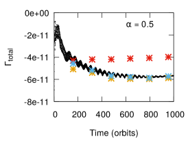
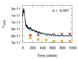
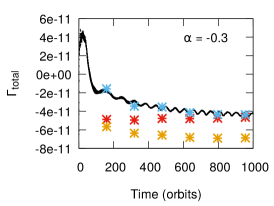
Figure 8: The total torque from the disk acting on the planet in the simulations with different $\alpha$. The orange asterisks show the torque expected from type I migration of the planet embedded in the locally-isothermal disk. The red and blue asterisks respectively indicate the torque obtained from Equation (13) and Equation (14).

5 The migration of two super-Earths capable of forming partial gaps

In the previous Section we have derived a phenomenological formula for the torque exerted on an isolated migrating super-Earth by the disk. In this Section we use this to aid with the interpretation of the migration in the two-planet case.

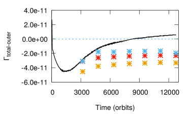
Figure 9: The total torque from the disk acting on the outer planet in the simulation with two super-Earths. The orange asterisks show our expectation of the torque from assumed type I migration of the outer planet embedded in the locally-isothermal disk. The red and blue asterisks indicate the torque calculated from Equation (13) and Equation (14) respectively.

In Figure 9, we present the torque $\Gamma_{\rm total-outer}$ from the disk acting on the outer planet in the numerical simulation with two super-Earths, migrating in a protoplanetary disk with the initial surface density given by Equation (2) with $\alpha=0.5$, $\Sigma_{0}=6\times 10^{-5}$, $h=0.02$ and $\nu=1.2\times 10^{-6},$ in order to see how the migration of the outer planet is affected by the presence of the second planet in the disk. In this figure we also show the torques calculated from Equation (10), Equation (13) and Equation (14) for the single migrating planet case derived in the previous Section.

We aim to compare the migration of the outer planet with and without the second planet in the disk. It is possible to do this only for times exceeding 3000 orbits, because at earlier stages of the evolution, $\alpha_{p},$ at the vicinity of the planet is outside the range covered by our single planet simulations. From this comparison we expect that if there is no second planet in the disk, the torque acting on the planet should remain negative till the end of the simulation. This is because the single planet always migrates inwards.

From the comparison we can also see that the torques calculated for the single planet case are less (though of larger magnitude) than what is seen in the two planet case. Moreover, at about 9000 orbits the torque in the two planet case becomes positive and the outer planet starts to migrate outwards. This means that in the two planets case, there is an additional mechanism by which angular momentum is transferred between the planets, either by direct gravitational interaction between them, and/or to the region in the vicinity of the outer planet and then to the outer planet itself. The first possibility is expected to be effective only very close to commensurability but we note that Baruteau & Papaloizou (2013) found that the mechanism still works when gravitational interaction between the planets was switched off in their simulations, indicating that something more is needed. The nature of the mechanism mentioned as the second possibility is connected with the wave planet interaction and will be explored in the next Section.

6 Coorbital torques for pairs of migrating planets with partial gaps

In this Section we will derive the scaling relation for effective repulsion due to wave planet interactions. In order to do this we begin by adopting an expression for the unmodified linear Lindblad torque induced by the unperturbed disk with background surface density, $\Sigma_{un},$ in the form

$$\Gamma_{L}=-3.075q^{2}\Sigma_{un}r^{4}\Omega^{2}h^{-2}.$$ (15)

Noting that this is insensitive to the form of the background surface density profile we remark that it is obtained from Equation (7) with the representative value $\alpha_{p}=1.$ Focusing on the inner planet, the net Lindblad torque is obtained by adding together the one sided Lindblad torques separately induced by the outer disk beyond the planet and the inner disk interior to it. From Papaloizou et al. (2007) we estimate that the outer one sided Lindblad torque is approximately given by $\Gamma_{L(1s)}=\Gamma_{L}/(5.7h).$ Thus we adopt

$$\Gamma_{L(1s)}=-0.54q^{2}\Sigma_{un}r^{4}\Omega^{2}h^{-3}.$$ (16)

Although we have focused on the outer one sided Lindblad torque due to the inner planet a corresponding situation applies, with a sign change to the inner one sided Lindblad torque due to the outer planet. Note that the associated angular momentum flow so considered is directed away from the planet and towards the other planet in each case and so will repel it as it approaches provided that it can absorb some of the angular momentum flowing towards it.

Consider another planet approaching the inner one from larger radii (smaller radii could equally well be considered). Outward propagating density waves dissipate in its coorbital region. Angular momentum is transfered to the horseshoe region and then to the planet through horseshoe drag. The effective angular momentum transfer rate can be estimated as

$$|\Gamma_{L(1s)}|2\lambda\sqrt{q_{2}/h}\sim 1.08\lambda\sqrt{q_{2}}q_{1}^{2}\Sigma_{un}r^{4}\Omega^{2}h^{-7/2},$$ (17)

where $q_{1}$ is the mass ratio of the emitting planet, here the inner one, $q_{2}$ is the mass ratio of the receiving planet, and we have assumed that a fraction $2\lambda x_{s}/r_{p}$ of the angular momentum flow is transferred to the horseshoe region of the receiving planet with $\lambda$ being a dimensionless constant, which we expect to be of order unity, as well as expression (5) for $x_{s}$. For this to be significant it should exceed the torques responsible for convergent migration. We estimate these to be of magnitude $f|\Gamma_{L}|$ for the emitting planet with $f$ being a dimensionless constant that can be of order but usually less than unity. Accordingly we require $|\Gamma_{L(1s)}|2\lambda\sqrt{q_{2}/h}\gtrsim f|\Gamma_{L}|$, or equivalently

$$\frac{q_{2}}{h^{3}}\gtrsim 8.1\left(\frac{f}{\lambda}\right)^{2}$$ (18)

As the right hand side of the inequality is characteristically around unity, indeed it becomes so for $f\sim\lambda/3,$ it has the same form as the thermal condition for nonlinearity and gap formation. Therefore the first condition for the effective wave planet interactions is of the same form as one required for the formation of a partial gap.

In the above discussion we limited consideration of transport of angular momentum brought in by waves to the horseshoe region. However, material just exterior to that may also transfer angular momentum to the planet through scattering. This may be incorporated within our simplified discussion by adopting a larger value for $\lambda.$ This would make our criteria easier to satisfy thus they would give a valid indication in this case also.

However, an issue of concern is that we used linear Lindblad torques whereas as indicated in Section 4.3 $x_{s}/r_{p}>2h/3$ for our simulations so we expect the torques to have been over estimated. As indicated in Section 4.3 we allow for this in an approximate manner by replacing $h$ by $3x_{s}/(2r_{1})$ with $x_{s}/r_{1}=\sqrt{q_{1}/h},$ and $r_{1}$ being the orbital radius of he inner planet when calculating $\Gamma_{L}$ and $\Gamma_{L(1s)}.$ Doing this (18) becomes simply

$$\frac{q_{2}}{q_{1}}\gtrsim 18.3\left(\frac{f}{\lambda}\right)^{2}$$ (19)

which will be satisfied for sufficiently slow convergent migration. This would appear to have no reference to partial gap formation. However (19) was derived under the condition $x_{s}>2H/3$ or $\sqrt{q_{1}/h^{3}}>2/3.$ If this is satisfied together with (19) we conclude that we must have

$$\frac{q_{2}}{h^{3}}>8.1\left(\frac{f}{\lambda}\right)^{2}$$ (20)

which is the condition implying a partial gap as before.

6.0.1 The value of $\lambda$

The condition (18) involves the quantity $\lambda.$ We recall that this was defined such that the fraction of the outward wave flux of angular momentum produced by the inner planet that is absorbed in the horseshoe region of the outer planet is $2\lambda\sqrt{q_{2}/h}.$ Thus if $\lambda=1,$ this corresponds to the flux being absorbed uniformly over a scale of the outer planet’s orbital radius, $r_{2},$ with the amount of absorption in any radial interval being proportional to its extent. However, in reality the flux is likely to decrease more rapidly with distance $x$ from the exciting planet. Dong et al. (2011) suggest that the flux $\propto x^{-5/4}.$ This implies that the fraction absorbed in the horseshoe region is $2.5\sqrt{q_{2}/h}(r_{2}/x)(L/x)^{5/4},$ where $L$ is the distance from the exciting planet beyond which the power law drop off is valid. In this context we remark that $L$ cannot be obtained from Dong et al. (2011) on account of nonlinearity near to the planet. Instead we shall assume $L=2x_{s},$ roughly corresponding to the gap width. Then the fraction absorbed is $5.2^{1/4}\sqrt{q_{2}/h}(r_{2}/x)(x_{s}/x)^{5/4}.$ In that case $\lambda~{}=~{}5.2^{-3/4}(r_{2}/x)(x_{s}/x)^{5/4}.$ Inserting $x_{s}/r_{1}=0.0243,$ the characteristic value for our simulations, and taking a separation corresponding to the 3:2 resonance, we obtain $\lambda\sim 0.56.$ Thus although there is considerable uncertainty $\lambda$ is plausibly of order unity for parameters of interest.

6.1 Effectiveness of the horseshoe drag

In addition to the above condition expressed by (18) we require that the material in the horseshoe region now in the gap region can transport the angular momentum deposited by waves to the planet through horeshoe drag. It is possible that material slightly exterior to the horseshoe region also transfers angular momentum brought in by waves through scattering and as we indicated above this may be incorporated by the choice of the value of $\lambda.$ In this situation less transport from the horseshoe region would be required than is assumed in this Section. Accordingly if the criteria for horseshoe regions to be effective developed below are satisfied we can be assured that they will be able to sustain the required transport.

In considering this we note that the strong density perturbation in the gap means that we need to think about this in a different way to that appropriate for the situation where there is no gap. We can consider the situation when the horseshoe drag is most effective. This is when it only works on one side of the planet. In the case of outward angular momentum transport towards the outer planet, which we focus on below, this will be that leading the planet. On the trailing side we suppose that material approaching the planet absorbs angular momentum from the waves causing the horseshoe turn to occur at significant distances from the planet. The one sided horseshoe drag results in

$$\Gamma_{hsl}=\frac{1}{2}\Sigma_{min}\Omega^{2}rx_{s}^{3}=\frac{1}{2}\Sigma_{min}\Omega^{2}r^{4}(q_{2}/h)^{3/2},$$ (21)

where $r$ and $\Omega$ are evaluated at the outer planet’s position with $\Sigma_{min}$ being the surface density at the gap minimum. Effective transfer to the outer planet can take place if

$$\Gamma_{hsl}>|\Gamma_{L(1s)}|2\lambda\sqrt{q_{2}/h}$$ (22)

or, recalling that $\Gamma_{L(1s)}$ is evaluated for the inner planet that equivalently

$$\left(\frac{\Sigma_{min}}{\Sigma_{un}}\right)_{2}>\left(\frac{2.16\lambda q^{2}_{1}}{q_{2}h^{2}}\right)\left(\frac{(\Sigma_{un}r^{4}\Omega^{2})_{1}}{(\Sigma_{un}r^{4}\Omega^{2})_{2}}\right),$$ (23)

where the subscripts $1$ and $2$ attached to brackets indicate the planet location for evaluation. We remark that we have used the linear Lindblad torque which, being an overestimate, will not disturb conclusions obtained from the above condition. In order to evaluate the second term enclosed in large brackets we assume that, as for our simulations, $-0.5<\alpha<0.5,$ and that the planets are close to 3:2 resonance in a Keplerian disk. Then this factor lies between $0.87$ and $0.67.$ Given that by definition $(\Sigma_{min}/\Sigma_{un})_{2}<1$, if the above condition is always satisfied we should have

$$\frac{1.9\lambda q^{2}_{1}}{q_{2}h^{2}}<1.$$ (24)

The two conditions we obtained for effective planet repulsion are (18) and (23). Here the wave generating planet has mass ratio $q_{1}$ and the receiving planet mass ratio $q_{2}$. Note that the roles may be reversed in which case we interchange $q_{1}$ and $q_{2}$ and the subscripts $1$ and $2$ in these conditions. While doing this we assume that the value of $\lambda$ remains the same.

In our calculations for $q_{1}=1.3\times 10^{-5}$ and $q_{2}=1.185\times 10^{-5}$ the requirement that $q_{2}/h^{3}=1.48>8.1(f/\lambda)^{2}$ is satisfied for $f\lesssim 0.43\lambda$ and also the second criterion is fulfilled, because, it is enough that $(\Sigma_{min}/\Sigma_{un})_{2}>0.052\lambda$, which is exactly the case if $\lambda$ does not exceed a factor of $\sim 4.$ If we apply the two criteria to the inner planet playing the role of the receiving planet then we obtain $1.6>8.1(f/\lambda)^{2}$, which is satisfied for $f\lesssim 0.44\lambda$. The second criterion in this case is

$$\left(\frac{\Sigma_{min}}{\Sigma_{un}}\right)_{1}>\left(\frac{2.16\lambda q^{2}_{2}}{q_{1}h^{2}}\right)\left(\frac{(\Sigma_{un}r^{4}\Omega^{2})_{2}}{(\Sigma_{un}r^{4}\Omega^{2})_{1}}\right),$$ (25)

This leads to the requirement that $(\Sigma_{min}/\Sigma_{un})_{1}>0.059\lambda$ to ensure it is satisfied for the range of $\alpha$ considered. This criterion is also satisfied for $\lambda$ not exceeding a factor of $\sim 4$ as above.

This means that in our calculations we should expect effective angular momentum transfer between the planets resulting from wave planet interactions, both from inner to outer planet and outer to inner planet can readily occur, particularly for slow enough convergent migration. We can also verify an additional consequence, namely reversing the planet positions, placing the inner one at the position of the outer planet and vice versa will lead to the same conclusion. Thus for either configuration repulsion due to wave planet interaction should be efficient. In the next Sections we will verify our prediction.

7 How does the migration depend on the mass of the planets?

For our particular choices of initial surface density profile we can study planet pairs with a range of mass ratios. We consider the mass ratios already discussed in detail, namely $q_{1}=1.3\times 10^{-5}$ and $q_{2}=1.185\times 10^{-5}$ with the initial surface density distribution being given by $\Sigma=\Sigma_{0}r^{-\alpha}$with $\alpha=0.5$ and $\Sigma_{0}=8\times 10^{-5}.$ For the same mass ratios we also ran a case with the initial surface density profile given by Equation (2) with $\alpha=0.5$ and $\Sigma_{0}=6\times 10^{-5}.$ In addition we perform simulations, starting with the latter initial surface density distribution and with the same value of $q_{2}$ but with $q_{1}$ respectively $1.185\times 10^{-5}$, $1.95\times 10^{-5}$ and $2.6\times 10^{-5}.$ This suite is completed by performing simulations with $q_{1}=1.185\times 10^{-5}$, $q_{2}=1.3\times 10^{-5}$ starting with the latter initial surface density distribution for two different values of $\Sigma_{0}$, namely $\Sigma_{0}=6\times 10^{-5}$ and $\Sigma_{0}=4.5\times 10^{-5}$.

Results are shown in Figure 10 in which we plot the position of both planets in each pair in the

$$\left[\frac{q_{1}}{h^{3}},\frac{h^{2}q_{1}}{\pi q_{2}^{2}}\left(\frac{\Sigma_{min}}{\Sigma_{un}}\right)_{1}\right]\hskip 2.84526pt{\rm and}\left[\frac{q_{2}}{h^{3}},\frac{h^{2}q_{2}}{\pi q_{1}^{2}}\left(\frac{\Sigma_{min}}{\Sigma_{un}}\right)_{2}\right]\rm{planes.}$$

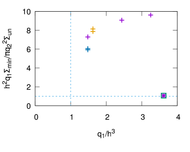
Figure 10: The results of the hydrodynamical simulations of two super-Earths migrating in a protoplanetary disk shown in the planes indicating the effectiveness of the repulsion due to wave planet interactions (crosses). The asterisks and open squares indicates the results obtained by recalculating the simulations with the parameters given in Baruteau & Papaloizou (2013) for Uranus-mass planets. The left panel gives information about the case in which the inner planet with the mass ratio $q_{1}$ is viewed as the receiver of waves emitted by the outer planet. The right panel gives information when the role of the planets in the pair is reversed, namely the outer planet is regarded as a receiver of waves emitted by the inner planet. See text for more details.

The left panel of Figure 10 showing the former gives information about the inner planet with the mass ratio $q_{1}$ as a receiver of waves emitted by the outer planet. The right panel showing the latter gives information when the role of the planets in each pair is reversed, namely it gives information about the outer planet regarded as a receiver of waves emitted by the inner planet.

Regarding the left hand panel we remark that the counterpart of the criterion given by (18) that is applicable to the inner planet will be satisfied for $f/\lambda<0.35$ if ${q_{1}}/{h^{3}}>1$ indicating enough supply to it as receiver to enable the halting of convergent migration. Similarly the criterion $({h^{2}q_{1}})/({\pi q_{2}^{2}})\left({\Sigma_{min}}/{\Sigma_{un}}\right)_{1}>\lambda,$ recalling that we expect $\lambda$ to be of order unity, ensures that the condition (24) which indicates the effectiveness of the horseshoe drag for the inner planet is satisfied and the planets are near to the 3:2 resonance. Similar remarks apply to the right hand panel with the role of the planets reversed and with ${q_{1}}/{h^{3}}$ and $({h^{2}q_{1}})/({\pi q_{2}^{2}})\left({\Sigma_{min}}/{\Sigma_{un}}\right)_{1}$ being respectively replaced by ${q_{2}}/{h^{3}}$ and $({h^{2}q_{2}})/({\pi q_{1}^{2}})\left({\Sigma_{min}}/{\Sigma_{un}}\right)_{2}.$ The regions delineated by the dashed lines which extend to large distances from the origin in each panel are thus locations where wave planet interaction can be effective.

The two orange crosses in each panel indicate the results obtained from the two simulations performed with the mass ratios $q_{1}=1.3\times 10^{-5}$ and $q_{2}=1.185\times~{}10^{-5}.$ For each panel the upper orange cross indicates the simulation in which the two planets are placed in the disk with the initial surface density distribution with $\Sigma=\Sigma_{0}r^{-\alpha}$ with $\alpha=0.5$ and $\Sigma_{0}=8\times 10^{-5}$. The lower one is the outcome of the simulation with the initial surface density profile given by Equation (2) with $\alpha=0.5$ and $\Sigma_{0}=6\times 10^{-5}$. The difference in the location of the crosses reflects the difference in the depths of the gaps.

The two turquoise crosses (in the left panel) and apparently one but in fact there are actually two overlapping each other in the right panel illustrate the results of the simulations with $q_{1}=1.185\times 10^{-5}$, $q_{2}=1.3\times 10^{-5}$ and two different values of $\Sigma_{0}$, namely $\Sigma_{0}=6\times 10^{-5}$ (the lower turquoise cross in the left panel) and $\Sigma_{0}=4.5\times 10^{-5}$ (the upper turquoise cross in the left panel). In both cases, the depth of the gap made by the planet with $q_{2}=1.3\times 10^{-5}$ is the same. That is why in the right panel one can see only one turquoise cross.

The three violet crosses show the remaining simulations for which effective repulsion due to wave planet interactions takes place. These three simulations only differ in the choice of the mass ratio of the inner planet which takes values $q_{1}=1.185\times 10^{-5}$, $1.95\times 10^{-5}$ and $2.6\times 10^{-5}$ respectively. It is interesting that as the mass ratio of the inner planet increases the depth of the gap it produces becomes larger and the depth of the gap the outer planet produces decreases, even though its mass ratio in all three cases is the same.

The position of the points in the planes discussed here is mostly determined by the mass ratios of the planets. In the left panel the location of the violet crosses increases from the left to the right following the increasing mass ratio of the inner planet. In the right panel, the violet crosses form a vertical line as $q_{2}$ is the same for all of them. Those with larger $q_{1}$ are located below those with smaller $q_{1}.$ The above results indicate that as $q_{1}$ increases for fixed $q_{2}$ the horseshoe drag on the inner planet is increasingly able to sustain the wave planet interaction. On the other hand the increasing Lindblad torques it produces make it harder for the outer planet to sustain the interaction at fixed $q_{2}.$ However, the reaction to this is likely to be that the disk planet interaction can be sustained with the planets being further apart.

According to our criteria, these planet pairs should eventually migrate divergently if they approach close enough to each other and the convergent migration causing this is slow enough. This is expected for all our hydrodynamic simulations.

7.1 The relationship to previous work

In order to make a clear link with the previous studies by Baruteau & Papaloizou (2013) we have recalculated the migration of two planets presented in their paper with mass ratios $q_{1}=4.4\times 10^{-5}$ and $q_{1}=4\times 10^{-5}$. The planets evolving in the disk with the initial surface density given by $\Sigma=\Sigma_{0}r^{-\alpha}$ with $\alpha=0.5$ and $\Sigma_{0}=8\times 10^{-5}$ enter into the 3:2 mean-motion resonance first and later on undergo divergent relative migration. The same planets evolving in the lower surface density disk with $\Sigma_{0}=3\times 10^{-5}$ become locked in the 2:1 commensurability and do not show signs of divergent migration. The results corresponding to $\Sigma_{0}=8\times 10^{-5}$ (violet asterisk) and $\Sigma_{0}=3\times 10^{-5}$ (green empty square) are also plotted in Figure 10. The criterion expressed by (18) and its counterpart corresponding to exchanging the planets are easily satisfied in both runs. Both planets create a partial gap. The second criterion corresponding to (24) with $\lambda=1$ and its counterpart corresponding to interchanging the planets are only just satisfied in the case eventually undergoing divergent migration with the criterion for the outer planet to be an effective receiver marginally failing when $\lambda=1$ for the case that retained convergent migration. So the results of a previous study are fully consistent with the picture presented here.

8 The effectiveness of repulsion resulting from wave planet interaction

We now go on to check the conditions under which we expect divergent migration of two super-Earths in the disk. In the previous Section we indicated that all the cases considered there were likely to exhibit effective repulsion due to wave planet interaction on the basis of our simple criteria based on the magnitude of wave fluxes and the potential of the horseshoe drag to communicate the angular momentum transported to the planet and we aim to verify this.

8.1 Dependence on the rate of convergent migration

We begin by comparing three particular cases. These form a sequence whereby the rate of initial convergent migration is increasing and either planet may have the largest mass ratio. Thus we are able to study how the location where the transition between convergent and divergent migration occurs depends on this. The cases we consider are one with the inner planet more massive than the outer one with $q_{1}=1.3\times 10^{-5}$, $q_{2}=1.185\times 10^{-5}$ (this case was already discussed in Section 3), the equal mass case with $q_{1}=q_{2}=1.185\times 10^{-5}$, and one for which the inner planet is less massive than the outer one with $q_{1}=1.185\times 10^{-5}$, $q_{2}=1.3\times 10^{-5}.$

In all cases the initial surface density was given by Equation (2) with $\alpha=0.5$ and $\Sigma_{0}=6\times 10^{-5}.$ The period ratio of the two planets as a function of time for these simulations is illustrated in Figure 11.

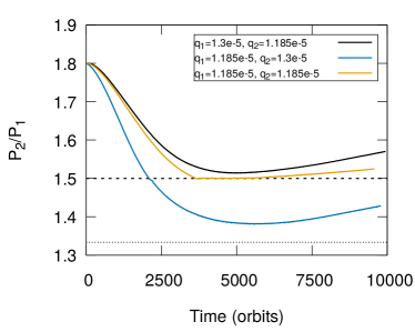
Figure 11: The period ratio of the two planets as a function of time for the hydrodynamical simulations of two super-Earths with mass ratios of $q_{1}=q_{2}=1.185\times 10^{-5}$ (orange line), $q_{1}=1.185\times 10^{-5}$, $q_{2}=1.3\times 10^{-5}$ (dark blue line) and $q_{1}=1.3\times 10^{-5}$, $q_{2}=1.185\times 10^{-5}$ (black line) migrating in a protoplanetary disk. The horizontal dashed and dotted lines respectively indicate the locations of the 3:2 and 4:3 resonances.

We have already described the case with $q_{1}=1.3\times 10^{-5}$ and $q_{2}=1.185\times 10^{-5},$ represented by the black line in Figure 11 in Section 3. The system evolves towards the 3:2 resonance and at some point leaves the vicinity of the commensurability and migrates divergently until the end of the simulation. The other two cases are qualitatively similar.

The case with $q_{1}=q_{2}$ represented by the orange line in Figure 11 arrives at the 3:2 resonance, stays there for a longer period of time as compared to the previous case and eventually leaves the resonance with a slower divergent migration rate.

In the simulation in which $q_{2}>q_{1}$ represented by the dark blue line in Figure 11, the relative convergent migration at the beginning of the evolution is the fastest of the three. The relative migration rate is so fast that the system passes through the 3:2 commesurability, but later on, the migration starts to be divergent. This shows that a close approach to strict commensurability is not necessary in order to induce divergent migration, even though one might expect that the 4:3 resonance could have some effect here (see the bottom panel of Figure 12).

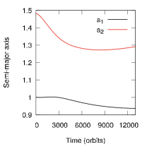
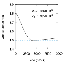
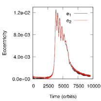
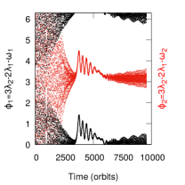
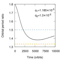
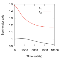
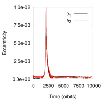
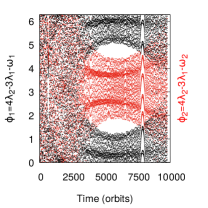
Figure 12: Each row shows the results of the simulations done with the same disk parameters, but different mass ratios of the planets. In the first row the mass ratios are $q_{1}=1.3\times 10^{-5}$, $q_{2}=1.185\times 10^{-5}$, in the second $q_{1}=q_{2}=1.185\times 10^{-5}$, and in the third one $q_{1}=1.185\times 10^{-5}$, $q_{2}=1.3\times 10^{-5}$. The panels in every row show the evolution of the planets’ orbital period ratio, semi-major axes, eccentricities and the resonance angles, as indicated on the rightmost panel, from left to right in each simulation. The horizontal dashed blue line in the first left panel in each row indicates the position of the 3:2 commensurability. The horizontal dashed yellow line indicates the position of the 4:3 resonance.

More detailed information from the three simulations is plotted in Figure 12. This includes the individual planet migration rates, the evolution of eccentricities and the behaviour of the resonance angles for either the 3:2 or 4:3 mean motion resonances where relevant. For completeness and convenience we present the results already displayed in Figure 3 in the uppermost row.

The second row shows the evolution of two equal mass planets with $q_{1}=q_{2}=1.185\times 10^{-5}.$ From the figure we see that before $t\sim 3500$ orbits the inner planet migrates slowly outwards due to the particular surface density profile adopted, while the outer planet migrates inwards. The convergent migration brings planets closer until the system arrives to the 3:2 MMR. The orbital period ratio of the two planets stays at around 1.5 until $t\sim 6000$ orbits. During this period, both planets migrate inwards. The eccentricities are excited to $\sim 0.012$ at $t\sim 4000$ orbits and subsequently decrease. One of the resonance angles associated with the 3:2 MMR is librating with mean value above $\pi$ that decreases with time, and the other with mean value in excess of zero that decreases with time. After $t\sim 6000$ orbits, the orbital period ratio of the planets is increasing slowly while the eccentricities continue to decrease. The resonance angles of the 3:2 MMR are librating with increasing amplitude. It is clear that the planets are leaving the 3:2 MMR.

The third row illustrates the case when the mass ratios of the two planets in the simulation illustrated in the uppermost row are interchanged. This has the effect of making the relative migration rate to be significantly faster. Thus it is not a surprise that in this case the relative migration is too fast to allow 3:2 resonance capture. Indeed, the planets passed through this resonance and at around 6000 orbits the migration becomes divergent. The 4:3 resonance may play a significant role. Note the distance from strict commensurability and the large amplitude librations of the resonance angles which occur around $6000$ orbits indicate a relatively weak effect though this could be enough to affect the evolution.

In summary, the three simulations illustrated in Figures 11 and 12 provide a sequence with increasing initial convergent migration rate. An increased rate is found to enable the pair to approach each other more closely before the relative migration reverses.

8.2 A slower initial convergent migration rate and faster subsequent divergent migration rate obtained by increasing $q_{1}$ at fixed $q_{2}.$

We now investigate how the evolution depends on the mass of the inner planet. In addition to those already discussed we have run another two simulations with $q_{1}=1.95\times 10^{-5}$ and $2.6\times 10^{-5}$ both of these having $q_{2}=1.185\times 10^{-5}.$ These enable us to consider a sequence of four simulations, in which the outer planet has the fixed mass ratio $q_{2}=1.185\times 10^{-5}$ with the inner planet respectively having the mass ratio $q_{1}=1.185\times 10^{-5}$, $1.3\times 10^{-5}$, $1.95\times 10^{-5}$ and $2.6\times 10^{-5}.$ For all of these cases the initial surface density distribution was given by Equation (2) with $\alpha=0.5$ and $\Sigma_{0}=6.0\times 10^{-5}.$

A comparison of the evolution of the orbital period ratio for these simulations is given in Figure 13 and additional details are presented in Figure 14.

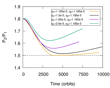
Figure 13: The results of the hydrodynamical simulations of two super-Earths with mass ratios $q_{1}=q_{2}=1.185\times 10^{-5}$ (orange), $q_{1}=1.3\times 10^{-5}$, $q_{2}=1.185\times 10^{-5}$ (black) and $q_{1}=1.95\times 10^{-5}$, $q_{2}=1.185\times 10^{-5}$ (violet) and $q_{1}=2.6\times 10^{-5}$, $q_{2}=1.185\times 10^{-5}$ (green) migrating in a protoplanetary disk.

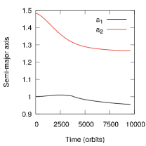
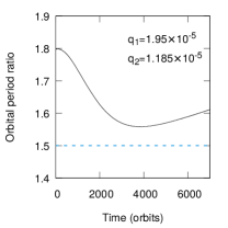
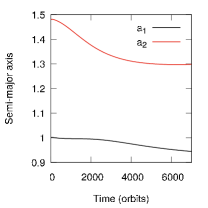
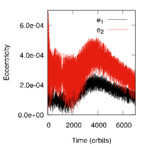
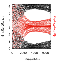
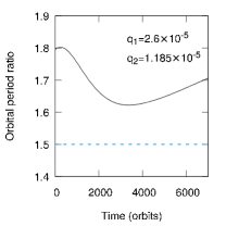
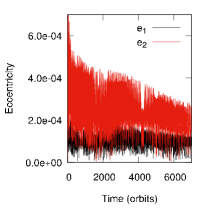
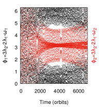
Figure 14: Each row shows the results of the simulations done with the same disk parameters and the mass ratio of the outer planet $q_{2}=1.185\times 10^{-5}$, but different mass ratios of the inner planet. In the first row the mass ratio of the inner planet is $q_{1}=1.185\times 10^{-5}$, in the second $q_{1}=1.3\times 10^{-5}$, in the third $q_{1}=1.95\times 10^{-5}$ and in the fourth $q_{1}=2.6\times 10^{-5}$. The panels in each row show the evolution of the planets’ orbital period ratio, semi-major axes, eccentricities and the resonance angles from left to right for each simulation. The horizontal dashed blue line in the leftmost panel in each row indicates the position of the 3:2 commensurability.

From Figure 13 we see that the initial relative migration rates in all four simulations are very similar but with a tendency to decrease as $q_{1}$ increases. This occurs because the surface density decreases sharply in the inner region of the disk, which tends to halt inward migration exactly where the inner planet is placed (see Equation (2)).

For the case where the inner planet has the lowest mass (orange line) the pair of super-Earths undergoes convergent migration and arrives at the position of the 3:2 resonance. However, stable resonance capture did not actually take place. This can be seen from the behaviour of the eccentricities of the planetary orbits displayed in the first row of Figure 14. When the resonance is first encountered the eccentricities are excited for a brief period before starting to decrease as the planets begin to undergo divergent migration.

Increasing the mass of the inner planet results in slower initial convergent migration. This leads to divergent migration sooner at a higher period ratio. In fact, the planets do not have a close approach to the 3:2 resonance. The migration of the outer planet in all cases except the equal mass simulation with $q_{1}=q_{2}=1.185\times 10^{-5}$, at some point reverses direction bringing the planet further away from its host star. It is likely that this would also happen in the simulation with two equal planets if we had continued the simulation for a longer time.

We have confirmation of the prediction that we should observe divergent migration in all configurations of the super-Earth pairs discussed here. It is of interest to perform a quantitative analysis of the divergent migration obtained in our simulations and its dependence on the mass of the inner planet. One of the characteristic properties of the evolution is the value of the semi-major axis ratio of two planets at the moment of time at which the transition from convergent to divergent migration takes place. We denote this by $a_{\rm min}=(a_{2}/a_{1})_{\rm min}$. Another relevant quantity is the relative migration rate during divergent migration

$$\dot{a}_{\rm div}=\left(\frac{d(a_{2}/a_{1})}{dt}\right)_{\rm div}.$$ (26)

The value of $\dot{a}_{\rm div}$ has been determined as an average over the last 1500 orbits of evolution. This and $a_{\rm min}$ are given in Table 3 for each simulation. From this table we can see that when $q_{1}$ is larger, $a_{\rm min}$ and $\dot{a}_{\rm div}$ are larger, which means that a higher mass inner planet leads to a faster divergent migration rate even though the earlier convergent migration rate was slower. This is a natural expectation on account of the expected larger wave flux produced by a planet with larger $q_{1}.$

Table 3: The relative migration rate of two planets in simulations with different $q_{1}$.

$q_{1}$	$a_{\rm min}$	$\dot{a}_{\rm div}$
($M_{\star}$)		($\rm yr^{-1}$)
$1.185\times 10^{-5}$	1.310	$3.954\times 10^{-6}$
$1.3\times 10^{-5}$	1.319	$9.263\times 10^{-6}$
$1.95\times 10^{-5}$	1.344	$1.235\times 10^{-5}$
$2.6\times 10^{-5}$	1.381	$1.627\times 10^{-5}$

8.3 Reducing the rate of convergent migration by decreasing the surface density

We here explore the effect of reducing the initial convergent migration rate by reducing the surface density scale. To do this we consider an additional simulation for which the planets have mass ratios $q_{1}=1.185\times 10^{-5}$ and $q_{2}=1.3\times 10^{-5}$ but with the lower surface density scale with $\Sigma_{0}=4.5\times 10^{-5}.$ Results for a simulation with the same mass ratios and initial surface density profile, but scaled with $\Sigma_{0}=6\times 10^{-5}$ was already presented in Figure 11. It will be seen from that figure that in that case the migration was fast enough for the planets to be able to pass through the 3:2 resonance.

Our main motivation in performing the simulation with reduced surface density scale as we have already mentioned above, was to investigate the situation in which the outer planet is more massive than the inner one, and the relative migration rate is not too fast for 3:2 resonance capture to take place. We choose $\Sigma_{0}$ in such a way that the convergent migration rate of the planets is approximately the same as for the evolution of the planets with $q_{1}=1.3\times 10^{-5}$ and $q_{2}=1.185\times 10^{-5}$ illustrated in Figure 11.

In Figure 15 the evolution of the period ratio is shown for the simulation with reduced surface density scale (red line) together with that for the simulation with $q_{1}=1.185\times 10^{-5}$ and $q_{2}=1.3\times 10^{-5}$ and $\Sigma_{0}=6\times 10^{-5}$ illustrated in Figure 11 (dark blue line) and also the case with $q_{1}=1.3\times 10^{-5}$ and $q_{2}=1.185\times 10^{-5}$ and $\Sigma_{0}=6\times 10^{-5}$ (black line) can be seen in Figure 15. More details for the lower surface density case are shown in Figure 16.

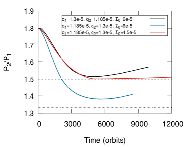
Figure 15: The results of the hydrodynamical simulations of two super-Earths with mass ratios of $q_{1}=1.185\times 10^{-5}$, $q_{2}=1.3\times 10^{-5}$ (dark blue) and $q_{1}=1.3\times 10^{-5}$, $q_{2}=1.185\times 10^{-5}$ (black) migrating in a protoplanetary disk with $\Sigma_{0}=6\times 10^{-5}$ together with the results for two super-Earths with mass ratios of $q_{1}=1.185\times 10^{-5}$, $q_{2}=1.3\times 10^{-5}$ migrating in the disk with $\Sigma_{0}=4.5\times 10^{-5}$ (red).

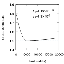
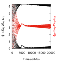
Figure 16: Results of the hydrodynamical simulation of two super-Earths with masses of $q_{1}=1.185\times 10^{-5}$ and $q_{2}=1.3\times 10^{-5}$ migrating in a protoplanetary disk. The initial surface density scaling with $\Sigma_{0}=4.5\times 10^{-5}$ is adopted in this simulation. Evolution of the planets’ orbital period ratio, semi-major axes, eccentricities and the resonant angles are shown in the panels from left to right. The horizontal dashed blue line in the leftmost panel indicates the position of the 3:2 commensurability.

As can be seen from Figure 16 at the beginning of this simulation the planets undergo convergent migration, at $t\sim 5000$ orbits, the orbital period ratio has decreased to close to 1.5 while the eccentricities of the planets attain maximum values $e_{1}=8.0\times 10^{-3}$ and $e_{2}=9.0\times 10^{-3}$. The 3:2 MMR resonance angles start to librate around values respectively slightly exceeding $0$ and $\pi$ with small amplitude. The period ratio stays close to 1.5 till $t\sim 7000$ orbits. At this time the eccentricities have decreased to $e_{1}=e_{2}\sim 4.0\times 10^{-3}$ and the centres of libration of the 3:2 MMR resonance angles shift to $0$ and $\pi.$

At $t\sim 7000$ orbits, the migration rates of both planets are decreasing, while the orbital period ratio is slowly increasing. The eccentricities decrease continuously at a progressively slower rate as $t$ increases. In addition the libration amplitudes of the resonance angles increases. From $t\sim{\color[rgb]{0,0,0}16000}$ orbits until the end of the simulation the outer planet migrates outwards.

In summary we find that in this case the planets enter into the 3:2 MMR, stay there for a couple of thousand of orbits and then slowly (slower than in the configuration with $q_{1}=1.3\times 10^{-5}$, and $q_{2}=1.185\times 10^{-5}$ in a protoplanetary disk with $\Sigma_{0}=6\times 10^{-5}$), moves away from the resonance. This is consistent with the notion that while the system remains close to the 3:2 commensurability the convergent migration is halted by the resonant interaction with the wave planet interaction not being strong enough to separate the planets. However, this changes as the migration rates slow down at later times and separation from the resonance can take place.

9 The mechanism at work and the importance of the horseshoe drag

In this Section we take closer look at the mechanism responsible for the repulsion between planets found in the hydrodynamical calculations. We return to one of our flagship cases, presented at the beginning of the present paper, namely two super-Earths with $q_{1}=1.3\times 10^{-5}$ and $q_{2}=1.185\times 10^{-5}$ evolving in the disk with $h=0.02$, $\nu=1.2\times 10^{-6},$ the initial surface density profile determined by Equation (2) with $\Sigma_{0}=6\times 10^{-5}$ and $\alpha=0.5.$

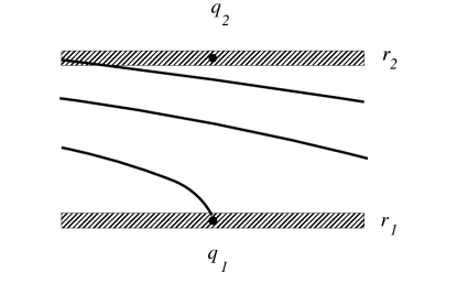
Figure 17: The schematic view of the scenario considered here: Two planets (black circles) with the planet-to-star mass ratios $q_{1}$ and $q_{2}$ embedded in the disk at the distances $r_{1}$ ad $r_{2}$ from the central star. The hatched regions along the orbits depict the horseshoe regions. The wave crests are associated with the density waves launched by the inner planet and are propagating outwards towards the horseshoe region of the outer planet where dissipation may occur.

9.1 The angular momentum flux associated with the planetary wakes

We have postulated that the repulsion between planets occurs due to the wave planet interaction. Outward propagating density waves excited by the inner planet dissipate in the coorbital region of the outer planet. The angular momentum carried by the waves is transfered to the horseshoe region and then to the planet through horseshoe drag (see Figure 17).

To demonstrate this, first, we calculate the angular momentum flux carried by density waves. The wave angular momentum flux as a function of $r$ has the form

$$F_{\rm wave}=r^{2}\bar{\Sigma}\int_{0}^{2\pi}(v_{\phi}-\bar{v}_{\phi})(v_{r}-\bar{v}_{r})d\phi$$ (27)

where $\bar{\Sigma}$ is the azimuthally averaged surface density defined as $\bar{\Sigma}=\frac{1}{2\pi}\int_{0}^{2\pi}\Sigma d\phi$ while $\bar{v}_{\phi}$ and $\bar{v}_{r}$ are the azimuthally averaged velocity in the azimuthal and radial direction, respectively. This is correct to second order in perturbations around the background state and should be adequate for the small amplitude waves considered. It is also important to note that this quantity, which we denote as a flux, represents the flow of angular momentum across a circle of radius, $r.$ The results for the flagship case are presented in the right panel of Figure 18 (black line).

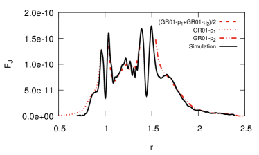
Figure 18: A comparison of the angular momentum flux calculated by Equation (27) (full line), and Equation (28) (dashed line) in the single planet case at t = 1000 orbits is shown in the left panel. A similar comparison is made for the two planet case in the (right panel). See the text for a description of the curves.

The wave flux $F_{\rm wave}$ shown in this figure has contributions from the wakes of two planets in the disk. Ideally, we would like to know what is the flux carried by the waves excited only by the inner planet, $F_{\rm wave-inner}$.

To estimate $F_{\rm wave-inner}$ we consider first a run with the same initial conditions as the flagship case but with the outer planet removed, we refer to this as the single planet case, and employ the expression given by Goodman & Rafikov (2001). According to them the angular momentum flux carried by the density wave constituting the wake of a planet in a non-self-gravitating disk is given by

$$F_{\rm J}(r)=\frac{c_{s}^{3}r_{p}^{2}}{|xrd\Omega/dr|\Sigma_{0}}\int_{-\pi}^{\pi}(\Sigma-\Sigma_{0})^{2}d\phi$$ (28)

where $x$ is the distance to the planet in the radial direction defined as $x=r-r_{p}$ and $\Sigma_{0}$ denotes the unperturbed surface density. In the left panel of Figure 18, we present a comparison of the angular momentum flux calculated by Equation (27) and Equation (28) for the simulation with a single planet in the disk. The agreement is very good. This shows that the wave flux generated by a single planet on its own is well represented by Equation (28).

Next, we calculate the angular momentum fluxes expected to be generated by the inner and outer planet separately and then combine them in a way that should represent the total angular momentum flux in a radial interval between the planets when the wakes do not interact and then compare this with Equation (27). The expression we use is given by

$$F_{\rm J}(r)=\left(\frac{r_{1}^{2}}{|x_{1}|}+\frac{r_{2}^{2}}{|x_{2}|}\right)\frac{c_{s}^{3}}{|2rd\Omega/dr|\Sigma_{0}}\int_{-\pi}^{\pi}(\Sigma-\Sigma_{0})^{2}d\phi,$$ (29)

where $x_{i}=r-r_{i}.$ We remark that there is a contribution of both wakes to the surface density in Equation (29) hence the factor of two in the denominator. We note that at the intermediate location where $r_{i}^{2}/x_{i}$ is the same for $i=1,2,$ given the result of the comparison in the single planet case, apart from possible contributions from small regions where the wakes cross, we should obtain the correct total angular momentum flux. The same is true more generally if the surface density perturbations from the wakes are nearly equal as is found to be the case near the midpoint of the interval between the planets. However, use of Equation (29) is likely to give an underestimate as gap edges are approached.

The results of the comparison of results obtained from Equation (27) (black curve), Equation (29) in the region between the planets (dashed red curve) and Equation (28) in the regions interior to the inner planet (dotted red curve) and exterior to the outer planet (double dot dashed red curve) for the two planet case are shown in the right panel of Figure 18.

We note that as expected, in the inner part of the disk, $F_{\rm wave}$ calculated by Equation (27) and the values obtained by applying the form of Equation (28) applicable to the inner planet, agree with each other. This is expected because in this region, the disk is mainly perturbed by the interior wake of the inner planet. Correspondingly, the outer part of the disk is mostly disturbed by the exterior wake of the outer planet and $F_{\rm wave}$ also agrees nicely with the values obtained from the form of Equation (28) applicable to the outer planet.

In the central part of the region, between two planets, the wakes of both planets perturb the disk with similar strength. Accordingly we found that $F_{\rm wave}$ is consistent with the contribution from the two planets expressed by Equation (29). Based on this comparison, we confirm that the angular momentum fluxes calculated from Equations (28) and (29) as applicable, which are based on the theoretical consideration of the effects arising from the planetary wakes, agree with the values of the angular momentum flux seen in our simulations.

9.2 The horseshoe region

Following the discussion in Section 6, the transfer of the angular momentum to the horseshoe region was expressed in terms of the angular momentum flow induced by a planet towards the other planet. Focusing on the transfer from the inner planet to the horseshoe region of the outer planet, we recall the expression for it given by the left hand side of Equation (17) in the form

$$\Gamma_{12hs}=|\Gamma_{L(1s)}|2\lambda\sqrt{q_{2}/h}$$ (30)

We can estimate this from the single planet run for which the left panel of Figure 18 illustrates the angular momentum flux produced by the inner planet when isolated. From this figure, we can see that the total angular momentum flux produced is $\sim 1.7\times 10^{-10}$ in code units and accordingly we estimate $\Gamma_{12hs}\sim 0.83\lambda\times 10^{-11}.$ The location of a 3:2 resonance with such a outer planet is at $r=1.31r_{1}.$ From Figure 18 we see that the angular momentum flux at this location is $\sim 2\times 10^{-11}.$ Referring back to Figure 9 which indicates the torque deficit between the actual torque and the expected type I torque acting on the outer planet in the two planet system, we see that this is also $\sim 2\times 10^{-11}.$ Thus we see there is consistency with the picture presented here of this deficit being supplied by the inner planet if the emitted flux that reaches the horseshoe region is mostly absorbed there and $\lambda\sim 2.4,$ being of order unity.

10 The effect of the planets on the evolution of the surface density and the slowing of the inward migration of the outer planet

In order to evaluate the effect of the planets in structuring the surface density profile of the disk, we illustrate the evolution of the surface density profile, $\Sigma(r,t),$ by plotting a sequence of surface density distributions obtained at different moments in time in our simulation with $q_{1}=1.3\times 10^{-5}$, $q_{2}=1.185\times 10^{-5}$ in the left panel of Figure 19. The initial surface density profile was determined by Equation (2) with $\alpha=0.5$ and $\Sigma_{0}=6\times 10^{-5}.$

For comparison, we report the evolution of the surface density $\Sigma(r,t)$ without the planets at the same moments in time in the right panel of Figure 19. Considering the evolution of the disk without planets, which is driven by the disk viscosity, we see that the maximum value of the surface density moves outwards, the trajectory being indicated by the dashed-dotted line in the figure. This has the consequence that the disk surface density profile becomes flatter as the evolution time increases.

In the disk with the embedded planets, the formation of partial gaps modifies the profile significantly. In particular, were the induced partial gaps to be filled in, the initial negative slope of the surface density distribution at the outer planet position can be seen to be transformed into a positive one. In addition the local maximum of the disk surface density that resides between the planets moves slightly inwards along with the migration of two planets.

By analogy with the operation of the horseshoe drag at a planet trap, the transformation to a positive surface density slope at the location of the outer planet might be expected to lead to a slowing down of its migration. Indeed it is notable that this occurs at a much earlier stage when compared to the evolution of the planets in a disk with the initial power law density profile which does not exhibit a positive slope on filling in the partial gaps (compare Figures 2 and 19). But note that this effect is not ultimately responsible for the divergent migration which eventually occurs in both systems.

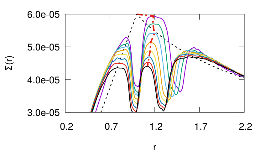
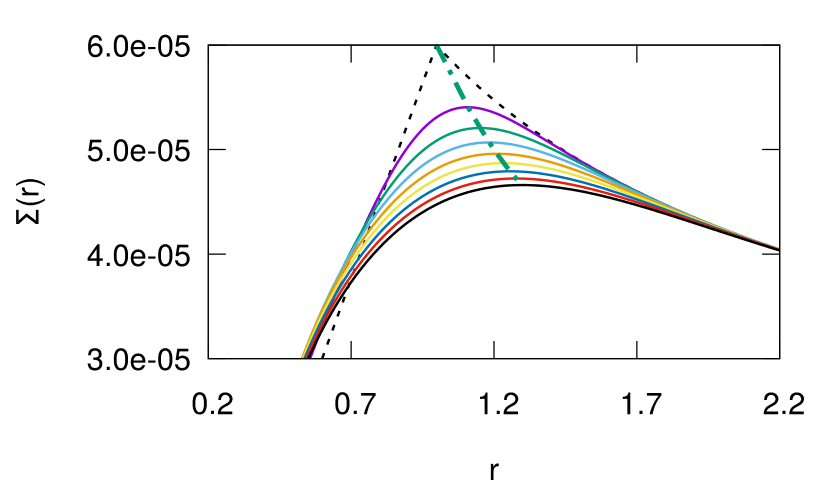
Figure 19: The surface density profile of the disk with $\Sigma_{0}=6\times 10^{-5}$ at each moment of time, with embedded planets with $q_{1}=1.3\times 10^{-5}$ and $q_{2}=1.185\times 10^{-5}$ (left panel), and without planets (right panel). The dashed black line indicates the initial surface density profile in the simulations. The solid lines show the surface density profiles at $t=796,1592,2389,3185,3981,4777,5573$ and $6369$ orbits respectively indicated with solid lines coloured in order from purple to black. The red dashed-dotted line in the left panel indicates the position of the local maximum of the surface density profile between the locations of the planets while the green dashed-dotted line in the right panel shows the position of the maximum of the surface density profile of the disk.

11 The dependence on the assumed equation of state and the effect of neglecting the self-gravity of the disk

In this Section we investigate the dependence on two assumptions made up to now in our simulations. These relate to the equation of state and the self-gravity of the disk

11.1 The equation of state

The equation of state prescribed the disk to be locally-isothermal. One aspect of this that has been noted by Miranda & Rafikov (2019) is that unlike when an adiabatic or barotropic equation of state applies, there is no strict conservation of wave action for small amplitude waves. There is accordingly the possibility of loss or gain from the background. We also expect coorbital torques to differ on account of different behaviour of the state variables within the horseshoe region. In order to check the influence of the equation of state on the results of our simulations, we have performed a simulation adopting an adiabatic equation of state. The conclusion based on this is that the generic outcome of the simulations remains unchanged independently of which equation of state is used. This means that in both cases repulsion between two planets caused by wave planet interaction is effective. Additional details and further discussion of this particular calculation are given in Appendix A.

11.2 Disk self-gravity

In the simulations described up to now, the self-gravity of the disk has been neglected, as the surface densities of the gas used in our simulations are relatively low corresponding to a Toomre $Q$ value $\sim 20.$ One of the effects of including disk self-gravity is to cause a shift of the location of Lindblad and corotation resonances, which leads to changes in the torques acting on a planet thus affecting its migration (see eg. Baruteau & Masset, 2008; Ataiee & Kley, 2020). In order to investigate the effect of self-gravity we have performed additional simulations described in detail in Appendix B. From the results of these we can infer that it is unlikely that self-gravity will have a significant influence on the results of our simulations.

12 The effect of a uniform surface density reduction on the Migration of two super-Earths

In Section 8.3 we explored the effect of modestly reducing the surface density scale on super-Earth pair migration finding that separation from resonance continues to take place. We investigated the situation in which the outer planet is more massive than the inner one, and the relative migration rate is not too fast for 3:2 resonance capture to take place. A reduction factor of 1.33 was sufficient for our purpose.

An issue arises as to whether the repulsion between planets described in the previous Sections will also be present in a disk with a much smaller surface density, scaled down 4 or even 16 times compared to that considered up to now. The motivation for this arises when we note that in the final stages of the evolution and dispersal of the protoplanetary disk the surface density is expected to decrease to significantly smaller values than expected for the minimum mass solar nebula.

We remark that there are good reasons for expecting that the character of the orbital evolution does not change with such a scaling. Noting that if the planets are on fixed orbits, the response induced in the disk will be proportional to the surface density scaling (the latter being everywhere scaled by the same constant factor). This is the case independently if self-gravity is not important (increasingly the case when the surface density is reduced) and also when the effect of self-gravity is investigated following the approach of Section 11.2 and Appendix B. This means that as long as the system is not in resonance the rate of orbital evolution of the planet resulting from disk-planet torques should also follow this scaling. Provided the response adjustment rate is fast compared to the orbital evolution rate, the latter should also follow the same scaling. Given that as shown by Baruteau & Papaloizou (2013) and Section 13 below the planet-planet repulsion mechanism works independently of the interaction between the planets we expect the procedure described here to be able to validate the orbital evolution rate scaling as well as confirm that planet planet interaction is not important in the later stages of the evolution as we find to be the case.

12.1 Numerical approach

Because following the complete planet evolution in a disk with a very low surface density is computationally expensive, we have adopted the following practical approach to study this question. The idea consists in starting new calculations with a rescaled surface density profile taken from one of our already performed simulations.The form and direction of the orbital evolution may then be checked at different stages and then pieced togetether.

For this purpose we select the surface density profile obtained at $t=10000$ orbits in the simulation shown in Figure 3. Next, we reduce $\Sigma$ at each grid point by a constant factor and then use such a density profile as the initial one for a new simulation.

Our choice of the time $t=10000$ orbits as the moment for restarting our calculation with a scaled down surface density was determined by the need to start the evolution when the torque from the disk acting on the outer planet is already positive (see Figure 9). We performed two new simulations, one with the surface density uniformly scaled down by a factor of 4 and another by a factor of 16. The initial surface density profiles in those two simulations are illustrated in Figure 20 together with the original $\Sigma(r)$ from which they have been obtained.

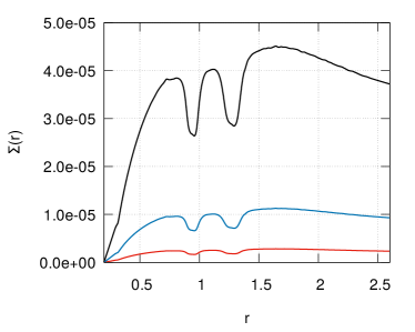
Figure 20: The azimuthally averaged surface density at t = 10000 orbits in the original simulation illustrated in Figure 3 (black line) and in the restarted ones with $\Sigma$ reduced by a factor of 4 (dark blue line) and by a factor of 16 (red line).

The evolution of planets in the disk with the surface density reduced by a factor of 4 and that with the surface density reduced by a factor of 16 is divergent just as it was in the original one shown in Figure 3. We illustrate this in Figure 21 showing the period ratio of the two planets in the restarted runs (left panels) together with the semi-major axes of the inner and outer planets (middle and right panels respectively). The outer planet in both cases migrates outwards and the inner one migrates inwards resulting in divergent migration. As expected the orbital evolution is four times faster in the case for which the initial surface density reduced by a factor of four.

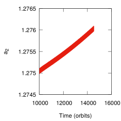
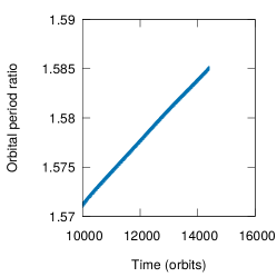
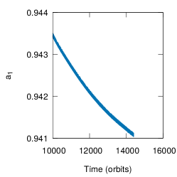
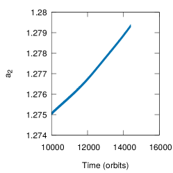
Figure 21: Left: The evolution of the period ratios of two super-Earths in the restarted simulation with the surface density reduced by a factor of 4 (indicated by the dark blue line) and 16 (indicated by the red line). Note that the evolution is four times slower in the former case and sixteen times in the latter; Middle and Right: Evolution of the semi-major axis of the inner and outer planets in the restarted simulation with surface density reduced by a factor of 4 (indicated by the dark blue line) and 16 (indicated by the red line).

As a final demonstration of the efficiency of the planet repulsion due to the wave planet interaction in the disk with a substantially reduced surface density, we present a comparison of the relevant torques in our simulations. In the left panel of Figure 22, we compare the torque from the disk acting on the outer planet in the simulations with the surface density reduced by a factor of 16 (red solid line) with the torque expected from a simple scaling procedure applied to the original calculation shown in Figure 3 (denoted by the dashed yellow line). The scaling procedure consists in decreasing the total torque by a factor of 16 and increasing the time scale of the orbital evolution by the same factor, as this time scale should scale inversely with the surface density. In addition, in order to compare the same phases of the evolution in both calculations the initial time for the lower density run is shifted to $t=160000$ orbits. The two torques are in very good agreement.

         

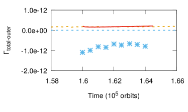
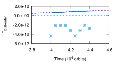
Figure 22: The locally time averaged total torque from the disk acting on the outer planet in the restarted simulations with the surface density respectively scaled down by a factor of 16 (left panel red solid line) and 4 (right panel dark blue solid line). For comparison the expected average total torques obtained by the appropriate scaling applied to the original simulation are denoted by the dashed yellow and purple lines in the left and right panels respectively. The blue asterisks indicate torques calculated from Equation (14).

In the right panel of Figure 22, we show the average torque in the run with the 4 times lower surface density (dark blue line) and the one expected from the scaling procedure described above (dashed purple line). Here the initial time for the low density calculation has been shifted to $t=40000$ orbits. These are in very good agreement. In Figure 22 we also show similar plots for the case when the surface density was reduced by a factor of 16 and the torques calculated from Equation (14), indicated by the blue asterisks.

One the basis of these results we can conclude that the repulsion of the planets is also present in the disks with a reduced surface density relative to that used in previous Sections.

13 Planets in the super-Earth mass range migrating in a protoplanetary disk with local heating and cooling

We have investigated the process of repulsion between planets arising from wave-planet interaction for a range of super-Earth masses and a range of values for the characteristic magnitude of the disk surface density. However, so far only a locally isothermal equation of state has been extensively considered. We now extend consideration to an initial disk model in which the balance between local heating and cooling determines the local disk temperature. This is very different from a local isothermal prescription and could potentially lead to substantially different dynamics in the vicinity of gaps induced by orbiting planets. The particular disk model adopted is viscous while initially supporting a constant angular momentum flux. As noted in Section 1 such a situation may arise when the inner disk interacts with a stellar magnetosphere prior to dispersal (eg. Clarke & Armitage, 1996). We remark that the magnetosphere may be associated with a protoplanet trap but we do not model this here.

13.1 A viscous protoplanetary disk with local balance between heating and cooling

Let us consider a model with constant angular momentum flux, $\cal{F}$, which reads

$${\cal F}=3\pi\nu\Sigma\sqrt{GM_{\star}r}$$ (31)

We adopt the general power law scalings with

$$\Sigma\propto r^{-\beta_{1}},\hskip 5.69054pth\propto r^{-\beta_{2}}\hskip 5.69054pt{\rm and}\hskip 5.69054pt\nu\propto r^{-\beta_{3}}.$$

To provide scalings for these quantities we set

$$\Sigma R^{2}/M_{\star}=6.0\times 10^{-5}f_{\Sigma}(r/R)^{-\beta_{1}}$$ (32)

$$h=0.02f_{h}(r/R)^{-\beta_{2}}\hskip 5.69054pt{\rm and}$$ (33)

$$\nu=1.2\times 10^{-6}f_{\nu}\sqrt{GM_{\star}R}(r/R)^{-\beta_{3}}$$ (34)

where we adopt the fixed parameters $M_{\star}=1M_{\odot}$ and the radius $R$ which determines that radial scale of the model to correspond to 0.1 au with $f_{h}$, $f_{\Sigma}$ and $f_{\nu}$ being dimensionless scaling constants expected to be of order unity. We remark that with the above specifications the characteristic disk mass within radius, $R,$ is $6\times 10^{-5}\pi f_{\Sigma}M_{\star}.$ For $R=0.1$ au, $M_{\star}=1M_{\odot}$ and $f_{\Sigma}=1$ this is about 1.5 times smaller than extrapolated for the minimum mass solar nebula. In this context we recall that this may be reduced by scaling down the surface density Then following the discussion in Section 12 we might expect that under appropriate conditions and scaling that the form of the disk planets interaction would be preserved. The constancy of ${\cal F}$ requires that $\beta_{1}+\beta_{3}=1/2$. Assuming a constant kinematic viscosity we have $\beta_{3}=0$ and thus $\beta_{1}=1/2.$ Using this and Equations (32) - (34), Equation (31) leads to

$$\frac{\cal F}{\sqrt{GM_{\star}R}}=1.35\times 10^{-7}f_{\nu}f_{\Sigma}M_{\odot}y^{-1}$$ (35)

To complete the model we need to consider the energy balance. This gives another relationship between the $\beta_{i}$. Thus together with the requirements specified above, these indices are completely specified. We start by considering the properties of the opacity. The opacity is mostly due to grains as can be seen from Ferguson et al. (2005). From their Figures 10 and 11, for the parameter ranges of interest the grain opacity is approximately constant and scales with metal abundance, $Z$, so that $\kappa\sim(Z/0.02)$. This scaling holds down to very small $Z$ as when $Z=0$, $\kappa\sim 10^{-8}$, which is associated with Rayleigh scattering due to Hydrogen molecules. Thus if there is significant unknown grain depletion as a result of the planet formation process, the opacity is highly uncertain translating to uncertainty in the disk models.

The surface density evaluated from Equation (32) assuming $M_{\star}=M_{\odot}$ and $R=0.1$ au is given by

$$\Sigma=53333f_{\Sigma}(r/R)^{1/2}$$ (36)

For standard metalicity (no grain depletion) this means that the disk is very optically thick with $\tau=5\times 10^{4}f_{\Sigma}$ at $r=R$.

In the optically thick case the rate of cooling per unit mass is given by

$$Q^{-}=(2\sigma T_{e}^{4})/\Sigma$$ (37)

where we assume that radial diffusion of heat is not important, this should be reasonable for disturbances on a radial scale exceeding the scale height with smaller scales being smoothed by physical and numerical viscosity, $\sigma$ is the Stefan-Boltzmann constant and $T_{e}$ is the effective temperature which has to be related to the mid-plane temperature. Let us consider the balance between viscous heating and cooling. The rate of viscous heating per unit mass $Q^{+}$ is given by

$$Q^{+}=\nu r^{2}\left(\frac{d\Omega}{dr}\right)^{2}=2.7\times 10^{-6}f_{\nu}(GM_{\star})^{3/2}R^{-5/2}(r/R)^{-3}$$ (38)

Equating this to $Q^{-}$ given above we can find $T_{e}$ which is expressed by

$$T_{e}^{4}=\frac{7.2}{\sigma}\times 10^{-2}f_{\nu}f_{\Sigma}(GM_{\star})^{3/2}R^{-5/2}(r/R)^{-7/2}$$ (39)

or

$$T_{e}=917.8(f_{\nu}f_{\Sigma})^{1/4}(r/R)^{-7/8}\ \rm{K}.$$ (40)

Next, we can consistently estimate $h$. Assuming that the mid-plane temperature $T=f_{T}T_{e}$, where $f_{T}$, is a scaling parameter (see below), we have

$$h=\frac{\sqrt{{\cal R}T/\mu}}{r\Omega}=0.019(f_{T})^{1/2}(f_{\nu}f_{\Sigma})^{1/8}(r/R)^{1/16}$$ (41)

where ${\cal R}$ is the gas constant and $\mu$ is the mean molecular weight. Here we adopt $\mu=2.35$ (see eg. Flaig et al. (2012)) corresponding to predominantly molecular Hydrogen.

The determination of $f_{T}$ depends on how energy is transported from the disk midplane to the surface. This is highly uncertain as the optical depth is affected by uncertain grain depletion and turbulent transport due to the magnetorotational instability operates. However, we remark that the simulations of Flaig et al. (2012) indicate only modest mean vertical variation of the temperature for models with optical depth $<\sim 100.$ Accordingly in order to have a working model, we shall assume appropriate grain depletion and adopt $f_{T}=1.$

Summarizing, the complete specification of the initial model is then

$$\Sigma R^{2}/M_{\star}=6.0\times 10^{-5}f_{\Sigma}(r/R)^{-1/2},$$ (42)

$$h=0.019f_{T}^{1/2}(f_{\nu}f_{\Sigma})^{1/8}(r/R)^{1/16}\hskip 8.53581pt{\rm and}$$ (43)

$$\nu=1.2\times 10^{-6}f_{\nu}\sqrt{GM_{\star}R}$$ (44)

For practical purposes we also set the scaling factors $f_{\Sigma}$ and $f_{\nu}$ equal to unity.

13.2 Numerical setup

We run simulations in which two planets are embedded in the disk with constant angular momentum flux described above (Equations (42 - 44)). As mentioned above, we adopt the unit of length $R$ = 0.1au and the unit of mas $M_{\star}=M_{\odot}$. The energy equation solved in the simulations is

$$\frac{\partial e}{\partial t}+\nabla\cdot(e{\bf{v}})=-P\nabla\cdot{\bf{v}}+Q^{+}\Sigma-Q^{-}\Sigma$$ (45)

where $e$ is the internal energy per unit area, ${\bf{v}}$ is the gas velocity, $P$ is the integrated pressure, $Q^{-}$ and $Q^{+}$ are the heating and cooling functions defined in Equations (37) and (38) respectively. An ideal equation of state is adopted which closes the hydrodynamic equations. Thus

$$P=\frac{{\cal R}}{\mu}\Sigma T.$$ (46)

The internal energy per unit area is then linked to the temperature through

$$e=\frac{{\cal R}}{\mu}\frac{\Sigma T}{\gamma-1}$$ (47)

where $\gamma$ is the adiabatic index is taken to be 9/7.

At this point we consider whether there is a surface density scaling down transformation of the type discussed in Section 12 that will preserve the disk response to planets in fixed orbits. In order for this to exist we see from Equation (45) the effective cooling rate must be similarly scaled down in order to preserve the form of the temperature. This could come about through assumed additional heating via reprocessing of radiation from the central star or an assumption that the disk transforms from being approximately of unit optical depth to becoming optically thin or a combination of these effects. Alternatively one could envisage that the disk becomes optically thicker through increasing the opacity with changing grain depletion as the surface density is scaled down.

We consider here an initial model with constant angular momentum flux, ${\cal F}$, for which the inner and outer boundaries correspond to imperfectly slippery rigid boundaries at which the constant flux is respectively transported away from and towards by viscous stresses. Thus in each case the boundary condition takes the form

$${\cal F}=-2\pi\nu\Sigma r^{3}\frac{d(v_{\phi}/r)}{dr},$$ (48)

where $v_{\phi}$ is the azimuthal component of the velocity. In our simulations we retain this boundary condition when the planets are introduced. In doing so we remark that the boundary conditions may evolve on a long time scale as physical conditions at the boundaries change. This requires greatly extended simulations that are a matter for future investigation.

13.3 A case with the equal mass planets

In the disk model described above, we locate two super-Earths with $q_{1}=q_{2}=2.6\times 10^{-5}$ at the initial positions of $r_{1}=1.0$ and $r_{2}=1.36$, respectively These radii are the initial radii of the planets expressed in units of $R$. From now on the general radius, $r,$ is also expressed in this unit. The disk was relaxed for 800 orbits in order to ensure convergence to the expected steady state before adding the planets to it. The evolution of the period ratio, semi-major axes, eccentricities and the resonant angles for this pair of planets are presented in Figure 23. Both planets migrate inwards. After a short initial period of divergent migration, the planets migrate convergently and at $t\sim$ 900 orbits they arrive at the 3:2 MMR. The eccentricities are excited to $e_{1}\sim 0.012$ and $e_{2}\sim 0.013$. The 3:2 resonant angles librate. When $t\sim 1300$ orbits, the planets start to migrate divergently, and their distance from exact commensurability increases. At later times, the eccentricities decrease and the resonant angles cease librating.

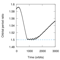
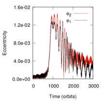
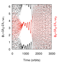
Figure 23: Results of the hydrodynamical simulation of two super-Earths with $q_{1}=q_{2}=2.6\times 10^{-5}$ migrating in the disk with local heating and cooling.

Next, we rerun the simulation but switch off the planet-planet interaction in the calculation. In this way, the influence of MMR, brought about through the gravitational influence of the planets on each other, on the migration of the planets is excluded. Rather we observe effects caused only by the interaction of planets with the gas in the disk structured by the wakes they produce. The orbital period ratio and the semi-major axes of two planets in this simulation are shown in Figure 24. These are respectively illustrated in the left and right panels.

Finally, we run two simulations in which only a single planet with $q=2.6\times 10^{-5}$ is put into the relaxed disk at the initial radii $r=1.0$ and $r=1.36$. The evolution of the semi-major axis of the planets are shown in the right panel of Figure 24. These are represented by the red solid and dashed lines. From the orbital periods $P_{1}$ and $P_{2}$ obtained from these two cases we calculate the period ratio $P_{1}/P_{2}$ and plot it in the left panel of Figure 24 where it is indicated by the red solid line.

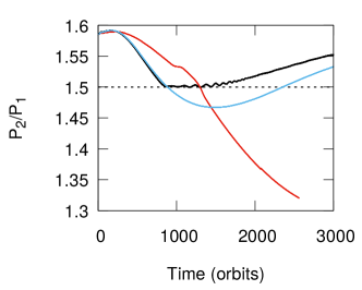
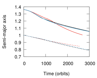
Figure 24: Left: Comparison of the period ratio evolution of the planets in the simulation of two super-Earths with $q_{1}=q_{2}=2.6\times 10^{-5}$ with (black solid line) and without (blue solid line) the planet planet interaction taken into account. The red solid line represents the period ratio calculated from the results of single planet runs for $q=2.6\times 10^{-5}$ starting from the initial positions $r=1.0$ and $r=1.36$. Right: Evolution of the semi-major axes of the two planets in the simulations shown in the left panel. The results of the simulations with and without the planet planet interaction are indicated by the black solid and dashed lines and the blue solid and dashed lines, respectively. The red dashed and solid lines represent the result of the single planet simulations initiated with $r=1.0$ and $r=1.36$, respectively.

The single planet with $q=2.6\times 10^{-5}$, initiated at $r=1.36$ migrates inwards. This is also the case when it is initiated at $r=1.00$. Moreover, the planet initiated at larger distance from the central star migrates faster than the one starting its evolution closer to the star. Knowing this, one predicts that the relative migration of a pair of such planets should be convergent. In this context we remark that temperature and surface density variations in the disk alone could produce divergent migration through their effect on the disk - planet interaction (see eg. Marzari & D’ Angelo, 2020). However, we do not find this here. Nonetheless convergent migration only persists for roughly 1000 orbits, at which point they enter into the 3:2 MMR, when the interaction between the planets is retained, or for 1500 orbits if we switch off the gravitational interaction between the planets. The former situation could be considered as an expected capture in the resonance, but the commensurability is not mantained and the planets migrate divergently, till the end of the simulation, as is also ultimately the case for which the interaction between the planets switched off. The ultimate divergent migration in the latter case must be produced by interaction with the perturbed disk with no resonant capture taking place. In this context we remark that the eccentricities of both planets are always small in this case

We have also performed a simulation for a case with $q_{1}=q_{2}=1.95\times 10^{-5}$. The convergent relative migration rate of two planets is slower at the beginning of the simulation in this case, which favours ultimate repulsion between the planets. Indeed, the planets are found to migrate divergently even before arriving at the 3:2 MMR. We will return to this case in a summary at the end of this Section.

13.4 A case with the unequal mass planets

Here, we perform a simulation in which the inner planet is less massive than the outer one. The inner planet has $q_{1}=1.3\times 10^{-5}$ and is initiated at $r_{1}=1.0$. The outer planet has the same value of $q_{2}=2.6\times 10^{-5}$ and the initial location $r_{2}=1.36$, as in our previous simulation. The same disk model as was adopted in the previous simulation was relaxed for 800 orbits before adding the planets .

The evolution of the period ratio, semi-major axes, eccentricities and the 4:3 resonant angles are illustrated in Figure 25. In this case, the early relative migration is convergent and much faster than in the equal planet case. As a consequence, the planets passed through the 3:2 MMR at about $t\sim$ 500 orbits and at $t\sim$ 1200 orbits they arrived at the 4:3 MMR. The eccentricities of the two planets get excited when the planets are passing through the 3:2 MMR and when arriving at the 4:3 MMR. After 3000 orbits, the period ratio is slowly increasing and the eccentricities slowly decreasing. Both 4:3 resonant angles librate until the end of the simulation. During the entire calculation, the inner and outer planets migrate inwards.

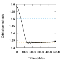
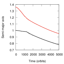
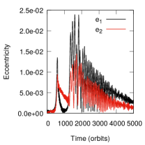
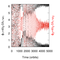
Figure 25: Results of the hydrodynamical simulation of the evolution of two super-Earths with $q_{1}=1.3\times 10^{-5}$ and $q_{2}=2.6\times 10^{-5}$ migrating in the disk with local heating and cooling.

As in the equal mass planet case, we ran a simulation in which the planet planet interaction is switched off. The orbital period ratio and the semi-major axes of the two planets in this simulation are shown in Figure 26. They are respectively indicated by the blue solid line in the left panel and the blue solid and dashed lines in the right panels. We also ran simulations for which single planets with $q=1.3\times 10^{-5}$ and $q=2.6\times 10^{-5}$ were inserted in the relaxed disk with the initial positions at $r=1.0$ and $r=1.36$, respectively.

The evolution of the semi-major axes of the planets in these simulations is shown in the right panel of Figure 26, and are represented by the red dashed and solid lines. Based on the orbital periods $P_{1}$ and $P_{2}$ respectively obtained from the single planet cases initiated with $r=1.0$ and $r=1.36$, we determine the period ratio $P_{1}/P_{2}$ and plot it in the left panel of Figure 26 where it is indicated by the red solid line.

When the planet-planet interaction was removed the early convergent migration was rapid enough to enable the planets to pass through the 4:3 and 5:4 commensurabilities. However, on approach to the 6:5 commensurability the migration became divergent and the period ratio subsequently increased slowly. This evolution is of the same character as that in the equal mass case.

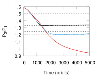
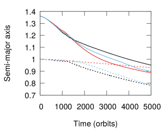
Figure 26: Left: Comparison of the period ratio of planets in the simulations of the evolution of two super-Earths with $q_{1}=1.3\times 10^{-5}$ and $q_{2}=2.6\times 10^{-5}$ migrating in a disk with local heating and cooling with and without the planet-planet interaction. These are respectively indicated by the black and blue solid lines while the red solid line represents the period ratio based on results from the single planet cases for $q=1.3\times 10^{-5}$ initiated at $r=1.0$ and $q=2.6\times 10^{-5}$ initiated at $r=1.36$. Right: Evolution of the semi-major axes of two planets in the simulations illustrated in the left panel. The results from the simulations with and without the planet planet interaction are respectively denoted by the black and blue dashed and solid lines. The red dashed and solid lines show the results of the single planet simulations with $q=1.3\times 10^{-5}$ and $q=2.6\times 10^{-5}$ respectively.

13.5 The effectiveness of the repulsion between planets in a disk with local heating and cooling

We have demonstrated the repulsion between planets with a mass in the super-Earth range in our simulations. This is due to the disturbance in the disk induced by one planet interacting with the other. As waves are launched by the planets in this interaction we describe this as wave planet interaction. The repulsion was found to be very strong between planets with equal mass as can be clearly noticed in Figure 27 (left panel). The initial relative migration in those cases is slow favouring the mechanism at work. We have applied the criteria for the effectiveness of the repulsion derived in Section 6 that were applied to our previous simulations, and plotted in Figure 10 (see the discussion in Section 7 for details), to the three simulations discussed here. The results are shown in Figure 27 (middle and right panels). They are consistent with the criteria we derived for the repulsion mechanism to work as they were for our previous simulations.

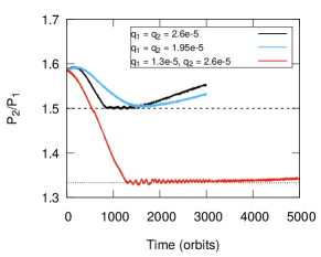
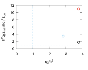
Figure 27: Left:The period ratio of the two planets as a function of time for the simulations of two super-Earths with mass ratios of $q_{1}=q_{2}=2.6\times 10^{-5}$ (black line), $q_{1}=q_{2}=1.95\times 10^{-5}$ (blue line) and $q_{1}=1.3\times 10^{-5},q_{2}=2.6\times 10^{-5}$ (red line) migrating in a disk with local heating and cooling. The horizontal dashed and dotted lines indicate the locations of the 3:2 and 4:3 resonances, respectively. Middle and Right: The results of the simulations illustrated in the left panel are plotted in the planes used to indicate the effectiveness of the repulsion due to wave planet interaction as was done for our prior simulations in Figure 10 (see the discussion in Section 7)

14 Discussion and Conclusions

In this paper we have demonstrated that wave planet repulsion can be effective in converting convergent migration to divergent migration as two planets in the super-Earth range, embedded in a thin low viscosity gaseous protoplanetary disk, approach a first-order commensurability. In Section 3 we found this for an inner planet with mass ratio $q_{1}=1.3\times 10^{-5}$ and an outer planet with mass ratio $q_{2}=1.185\times 10^{-5}$ in a disk with aspect ratio, $0.02,$ and kinematic viscosity, $1.2\times 10^{-6}.$ This occurred for both a power law surface density profile and one allowing for an inner cavity.

In order to exhibit effects arising solely because of the presence of two planets we performed simulations of an isolated outer planet in Section 4. Because in our simulations the planets always make partial gaps we found that standard type I migration does not apply even when scaled with the surface density in the gap. We developed a new fit to the migration rate applicable to local power law surface density profiles (Equation (14)). In Section 5 we used this result to show the presence of an additional torque acting on the outer planet, which we identified as being due to wave planet interaction, and characterised its magnitude.

A simplified description of wave planet interactions was developed in Section 6. This was based on density waves emitted by one planet being absorbed in the horseshoe region of the other and then transmitted to it, thus being able to supply an additional torque needed to change from convergent to divergent migration. Approximate conditions for this to be effective were given (criteria (20) and (23) and their counterparts for the other planet). These imply that the planets should be massive enough to make a partial gap but that this should not be so deep that there is inadequate material in horseshoe regions to be able to transfer the angular momentum transported by waves to the associated planet. They were verified for our simulations in Section 7 for a range of mass ratios $(1.185-2.6)\times 10^{-5}$ adopted for both planets.

We investigated the dependence of the rate of initial convergent migration in Section 8, showing that it increased on increasing the disk surface density or the mass ratio of the outer planet relative to the inner one. Increasing the initial rate of convergence resulted in the planets approaching each other more closely before switching to divergent migration.

In addition we checked that the angular momentum being transported between the planets was consistent with theoretical expectation in the case of density waves generated by the planets’ interaction with the disk in Section 9. It was also shown that this was consistent with the magnitude of the torque required to convert from convergent to divergent migration.

In Sections 10 - 12 we established the robustness of the mechanism to changes of the form of the surface density profile, changes to the equation of state and a correction to allow for the effect of self-gravity. In addition we investigated the effects of significant changes to the magnitude of the surface density in the disk in which the planets are embedded by considering reductions in this by more than an order of magnitude obtained through application of a uniform scaling factor. Finally in Section 13 we demonstrated the effectiveness of the repulsion between planets in a viscous disk in which the temperature was determined by a local balance between heating and cooling.

Thus we have investigated the mechanism underlying the repulsion between two planets migrating in the disk that enables the transition between convergent and divergent migration in some detail. It has been found that density waves emitted by the planets and the horseshoe drag play an important role in the process.

Significantly the phenomenon continues to occur when the gravitational interaction between the planets is omitted which supports this view. A close approach to strict commensurability is not necessary to induce divergent migration. However, the mean-motion resonances may play a significant role in the process of planet repulsion. Our findings provide one of the possible reasons, why there are not as many observed pairs of planets locked in strict mean-motion resonances, as could be inferred from discussions taking into account only standard type I migration. However, a full assessment requires an extensive study incorporating the entire final stages of the evolution of proptoplanetary disks that also incorporates the formation of the planets which we hope can be undertaken in future.

Appendix A The migration of two super-Earths in an adiabatic disk

For the adiabatic case we adopt the equation of state in the form

$$P=(\gamma-1)e\Sigma$$ (A1)

where, $P$ is the vertically integrated pressure, $\gamma$ is the adiabatic index and $e$ is the specific internal energy. As an objective is to probe the effect of there being strict wave action conservation for linear waves, we follow Miranda & Rafikov (2019) and set the value of $\gamma$ to be 1.001. On account of being close to unity. this has the effect that the equation of state approaches the limit in which the temperature is conserved on fluid elements. Physically in this limit the temperature does not change on account of the very large number of degrees of freedom within the gas. In this limit the temperature does not change in a Lagrangian sense in comparison with the locally-isothermal equation of state for which it does not change in an Eulerian sense.

The remaining details of the numerical setup are the same as in the flagship case for which $q_{1}=1.3\times 10^{-5}$ and $q_{2}=1.185\times 10^{-5}$ and the initial surface density profile was determined by Equation (2) with $\alpha=0.5$ and $\Sigma_{0}=6\times 10^{-5}$ (see Section 3.1). However, we do not used the killing-zone treatment near the boundaries of the disk in this simulation.

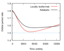
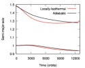
Figure 28: Left and middle: The orbital period ratio and semi-major axes of the two planets in the simulations with a locally-isothermal disk and an adiabatic equation of state. Right: The surface density profile in the vicinity of the outer planet in the simulations with a locally-isothermal disk (red lines) and the disk with an adiabatic equation of state (black lines) at t=3000, 6000 and 9000 orbits, these being respectively indicated by the dashed-dotted lines, solid lines and dashed lines.

In Figure 28, we show a comparison of the evolution of the orbital period ratio, semi-major axes of two planets and the surface density profile in the vicinity of the outer planet in the simulation with the locally-isothermal disk with the corresponding quantities obtained for the adiabatic case. It is clear that the two planets start to undergo divergent migration in the adiabatic case when the period ratio is around 1.58 at $t\sim 6000$ orbits. From a comparison of the orbital period ratios presented in the left panel of Figure 28, we can see that in the adiabatic disk, the divergent migration occurs later and when the distance between two planets is larger than in the locally-isothermal disk. As shown in the middle panel of Figure 28, the migration of the inner planet in both disks is similar while, the migration rate of the outer planet is slower in the adiabatic disk than in the locally-isothermal one. In the adiabatic case the outer planet migrates inwards till the end of the simulations, although at that stage it is very slow. While in the locally-isothermal case, it migrates outwards at the final stage of the calculation.

In the right panel of Figure 28, the surface density profiles at t=3000, 6000 and 9000 orbits in two cases are shown. It is clear that at t=3000 orbits, the surface density profiles in the vicinity of the outer planet in both simulations are similar, though their forms at the bottom of the partial gap opened by the planet differ slightly. The gap is slightly deeper in the locally isothermal case with difference between that and the adiabatic case being larger in the inner region of the gap. This is most noticeable at t=6000 orbits, when the divergent migration starts and at t=9000 orbits, in the adiabatic case, the maximum deviation of the surface density in the partial gap from that found in the locally-isothermal case still occurs in the inner region.

The above features indicate differing behaviour in the coorbital region associated with different temperature profiles (see the left panel of Figure 29). In the case of a locally isothermal equation of state the temperature profile is simply determined by location. On the other hand in the adiabatic case, in the limit $\gamma\rightarrow 1$, it will depend on the history of the material and possibly affected by phase mixing. The explicit comparison between those two cases at t=3000 orbits is shown in the left panel of Figure 29. When the adiabatic equation of state is adopted the temparature in the gaps is reduced below the background. This is expected if the planet migrates inwards dragging its horseshoe region with it. Another feature of the temperature profile, present beyond the outer gap edge, namely the increase of the temperature above the background, is due to the inner material passage through the separatrix to the outer disk. In the right panel of Figure 29 we present a contour plot of the temperature in the horseshoe region of the outer planet at t=3000 orbits. The conditions in the gap are very smooth indicating that viscous and numerical diffusion have dealt well with phase mixing in the horseshoe region making the temperature quite uniform. The features in the coorbital dynamics, described here, which are the consequences of the conservation of entropy lead to differences in the horseshoe drag that are not easy to determine and in turn to a different torque that we calculate. Indeed such effects seem to slow down the convergent migration of the system at an early stage in the adiabatic case leading to an onset of divergent migration at larger period ratios.

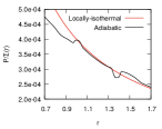
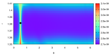
Figure 29: Left: The temperature profile in the vicinity of two planets at t = 3000 orbits in the simulations with a locally-isothermal disk and an adiabatic equation of state. Right: A contour plot of the temperature in the horseshoe region of the outer planet at t = 3000 orbits in the simulation with an adiabatic equation of state. The position of the planet is indicated by the black solid circle.

Appendix B The effect of disk self-gravity on the migration of the two super-Earths

In order to take account of the effect of self-gravity we follow the procedure of Benitez-Llambay et al. (2016) who found that this could be done by removing the azimuthally averaged surface density from the density of each cell prior to the calculation of the force due to self-gravity acting on the planet. This ensures that the background forces acting on the background rotating disk and planets are applied in a consistent manner.

Accordingly we run another simulation, in which all the numerical parameters are the same as adopted previously in the case of a single planet with $q=1.185\times 10^{-5}$ evolving in a locally isothermal disk with $\alpha=0.5$ starting with the surface density profile given by Equation (2) with $\Sigma_{0}=6\times 10^{-5},$ $h=0.02$ and $\nu=1.2\times 10^{-6}.$ Results for that case have already been presented in Figure 8. In this case the difference is that the forces acting on the planet are evaluated according to the procedure of Benitez-Llambay et al. (2016) outlined above.

The evolution of the semi-major axis and the torque acting on the planet in this run are shown in Figure 30. For comparison, the results of the simulation for the single planet case with $\alpha=0.5$ shown in Figure 8 are also shown in this figure.

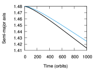
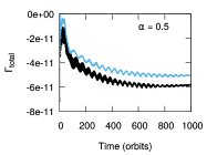
Figure 30: Left: The evolution of the semi-major axis of the single planet in the non-self-gravitating disk (black line) and with the correction to allow for the effect of the disk self-gravity (blue line). Right: The torque from the disk acting on the planet in both cases.

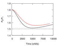
Figure 31: The orbital period ratio of the planets in the non-self-gravitating disk (black line) and with the correction to allow for the effect of the disk self-gravity (red line).

From Figure 30, it is clear that after applying the procedure to account for self-gravity, the migration of the planet in the disk is slightly slower than in the previous case. The total torque from the disk acting on the planet after 700 orbits is $\Gamma_{\rm total}\sim-5\times 10^{-11}$ while in the case without the correction the total torque is around $-6\times 10^{-11}$. From this comparison, we see that the effect of introducing the new procedure is similar to what would be attained by reducing the background surface density by a modest amount and thus could be compensated for by increasing it (see the discussion Section 8.3).

After investigating the effect of disk self-gravity on the migration of a single planet we are quite confident that taking into account this effect in the two-planet case will not change qualitatively the outcome of our calculations. To demonstrate this, we perform the simulations for our flagship run (see Section 3.1 ) again, but this time implementing the same procedure as described above for a single planet. The results are shown in Figure 31 (red line) together with the original flagship case (black line). In this figure, we show a comparison of the evolution of the orbital period ratios in both simulations. It is clear that the divergent migration occurs later when the self-gravity is taken into account. In addition, the divergent migration takes place when the distance between two planets is larger than in the disk without self-gravity included. The observed effect of disk self-gravity is similar to that obtained by reducing the background surface density, as illustrated in Figure 15 and discussed in Section 8.3.

References

- Ataiee & Kley (2020) Ataiee, S., Kley, W. 2020, A&A, 635, A204
- Baruteau & Masset (2008) Baruteau, C., Masset, F. 2008, ApJ, 678, 483
- Baruteau & Papaloizou (2013) Baruteau, C., Papaloizou, J.C.B. 2013, ApJ, 778, 7
- Batygin & Morbidelli (2013) Batygin, K., Morbidelli, A. 2013, AJ, 145, 1
- Benitez-Llambay & Masset (2016) Benitez-Llambay, P., Masset, F.S. 2016, ApJS, 223, 11
- Benitez-Llambay et al. (2016) Benitez-Llambay, P., Ramos, X.S., Beauge, C., Masset, F.S. 2016, ApJ, 826, 13
- Carter et al. (2012) Carter, J.A., Agol, E., & Chaplin, W.J., et al. 2012, Science, 337, 556
- Clarke & Armitage (1996) Clarke, C.J., Armitage, P.J., 1996, MNRAS, 280, 458
- Crida et al. (2006) Crida, A., Morbidelli, A., Masset, F. 2006, ICARUS, 181, 587
- Delisle & Laskar (2014) Delisle, J.B., Laskar, J. 2014, A&A, 570, L7
- de Val-Borro et al. (2006) de Val-Borro, M., Edgar, R.G., & Artymowicz, P., et al. 2006, MNRAS, 370, 529
- Dong et al. (2011) Dong, R., Rafikov, R.R., Stone, J.M., Petrovich, C. 2011, ApJ, 741, 56
- Duffell et al. (2014) Duffell, P.C., Haiman, Z., MacFadyen, A.I., D’Orazio, D.J., Farris, B.D. 2014, ApJL, 792, L10
- Dürmann & Kley (2015) Dürmann, C., Kley, W. 2015, A&A, 574, A52
- Dürmann & Kley (2017) Dürmann, C., Kley, W. 2017, A&A, 598, A80
- Fabrycky et al. (2014) Fabrycky, D.C., Lissauer, J.J., & Ragozzine, D., et al. 2014, ApJ, 790, 146
- Ferguson et al. (2005) Ferguson, J. W., Alexander, D. R., Allard, F., Barman, T., Bodnarik, J. G., Hauschildt, P.H., Heffner-Wong, A. & Tamanai, A., 2005, ApJ623, 585
- Goodman & Rafikov (2001) Goodman, J., Rafikov, R.R. 2001, ApJ, 552,793
- Hadden & Lithwick (2016) Hadden, S., Lithwick, Y. 2016, ApJ, 828, 44
- Hadden & Lithwick (2017) Hadden, S., Lithwick, Y. 2017, ApJ, 154, 5
- Flaig et al. (2012) Flaig, M., Ruoff, P., Kley, W., Kissmann, R. 2012, MNRAS 420, 2419
- Jontof-Hutter et al. (2016) Jontof-Hutter, D., Ford, E.B., Rowe, J.F. 2016, ApJ, 820, 39
- Kanagawa et al. (2018) Kanagawa, K., Tanaka, H., Szuszkiewicz, E. 2018, ApJ, 835, 140
- Kanagawa & Szuszkiewicz (2020) Kanagawa, K., Szuszkiewicz, E. 2020, ApJ, 894, 59
- Kley et al. (2004) Kley, W., Peitz, J., Bryden, G. 2004, A&A, 414, 735
- Kley & Nelson (2012) Kley, W., Nelson, R.P. 2012, Annual Review of Astronomy and Astrophysics , 50, 211
- Korycansky & Papaloizou (1996) Korycansky, D. G., Papaloizou, J.C.B. 1996, ApJS, 105, 181
- Lee et al. (2013) Lee, M.H., Fabrycky, D., Lin, D.N.C. 2013, ApJ, 774, 52
- Lin & Papaloizou (1979) Lin, D.N.C., Papaloizou, J.C.B. 1979, MNRAS, 186, 799
- Lin & Papaloizou (1993) Lin, D.N.C., & Papaloizou, J.C.B. 1993, Protostars and Planets III (Univ. of Arizona Press, Tucson, AZ)
- Lissauer et al. (2011) Lissauer, J.J., Ragozzine, D., & Fabrycky, D.C., et al. 2011, ApJ, 197, 8
- Lithwick & Wu (2012) Lithwick, Y., Wu, Y. 2012, ApJ, 756, L11
- Marzari & D’ Angelo (2020) Marzari, F., D’ Angelo, G., 2020, A&A, 641, 125
- Masset et al. (2006) Masset, F.S., Morbidelli, A., Crida, A., Ferreira, J. 2006, ApJ, 642, 478
- Miranda & Rafikov (2019) Miranda, R., Rafikov, R.R. 2019, ApJ, 878, L9
- Nelson & Papaloizou (2002) Nelson, R.P., Papaloizou, J.C.B. 2002, MNRAS, 333, 26
- Paardekooper & Papaloizou (2009) Paardekooper, S.J., Papaloizou, J.C.B. 2009, MNRAS, 394, 2283
- Paardekooper et al. (2010) Paardekooper, S.J., Baruteau, C., Crida, A., Kley, W. 2010, MNRAS, 401, 1950
- Papaloizou & Lin (1984) Papaloizou, J.C.B., Lin, D.N.C. 1984, ApJ, 285, 818
- Papaloizou & Szuszkiewicz (2005) Papaloizou, J.C.B., Szuszkiewicz, E. 2005, MNRAS, 363, 153
- Papaloizou et al. (2007) Papaloizou, J.C.B., Nelson, R.P., Kley, W., Masset, F.S., & Artymowicz, P. 2007, Protostars and Planets V, 655 (University of Arizona Press, Tucson)
- Papaloizou & Terquem (2010) Papaloizou, J.C.B., Terquem, C. 2010, MNRAS, 405, 573
- Papaloizou (2011) Papaloizou, J.C.B. 2011, Celest. Mech. Dyn. Astron., 111, 83
- Podlewska-Gaca et al. (2012) Podlewska-Gaca, E., Papaloizou, J.C.B., Szuszkiewicz, E. 2012, MNRAS, 421, 1736
- Saad-Olivera et al. (2020) Saad-Olivera, X., Martinez, C.F., Costa de Souza, A., Roig, F., Nesvoruy, D. 2020, MNRAS, 491, 5238
- Shakura & Sunyaev (1973) Shakura, N.I., Sunyaev, R. A. 1973, A&A, 24, 337
- Steffen & Hwang (2015) Steffen, J.H., Hwang, J. A. 2015, MNRAS, 448, 1956
- Vissapragada et al. (2020) Vissapragada, S., Jontof-Hutter, D., & Shporer, A., et al. 2020, AJ, 159, 108