The SMART protocol – Pulse engineering of a global field for robust and universal quantum computation

Abstract

Global control strategies for arrays of qubits are a promising pathway to scalable quantum computing. A continuous-wave global field provides decoupling of the qubits from background noise. However, this approach is limited by variability in the parameters of individual qubits in the array. Here we show that by modulating a global field simultaneously applied to the entire array, we are able to encode qubits that are less sensitive to the statistical scatter in qubit resonance frequency and microwave amplitude fluctuations, which are problems expected in a large scale system. We name this approach the SMART (Sinusoidally Modulated, Always Rotating and Tailored) qubit protocol. We show that there exist optimal modulation conditions for qubits in a global field that robustly provide improved coherence times. We discuss in further detail the example of spins in silicon quantum dots, in which universal one- and two-qubit control is achieved electrically by controlling the spin-orbit coupling of individual qubits and the exchange coupling between spins in neighbouring dots. This work provides a high-fidelity qubit operation scheme in a global field, significantly improving the prospects for scalability of spin-based quantum computer architectures.

I Introduction

Large-scale fault-tolerant quantum computing requires a robust and readily scalable qubit architecture, including initialisation, manipulation and measurement capabilities, with error rates below 1 % Knill (2005); Fowler et al. (2012). This implies that high-performance qubit gates and, ultimately, long qubit coherence times are required. Several demonstrations of qubit fidelities $>99\,\%$ exist for small-scale qubit systems Muhonen et al. (2015); Watson et al. (2018); Yoneda et al. (2018); Yang et al. (2019); Harty et al. (2014); Chow et al. (2009); Rong et al. (2015); Barends et al. (2014), however a major obstacle on the way to realising a practical large-scale quantum computer is the challenge of scaling up architectures while maintaining high fidelities.

One strategy explored in the literature to overcome this problem is the electromagnetic dressing of qubits. By constantly driving the qubit, one can prolong the coherence times by continuously refocusing qubits against slow fluctuations in Rabi frequency Timoney et al. (2011); Laucht et al. (2017); Wu et al. (2019); Cai et al. (2012). In addition, this is a scalable control scheme, since the driving microwave field can be applied globally to the entire multi-qubit device Kane (1998); Veldhorst et al. (2017); Seedhouse et al. (2021); Vahapoglu et al. (2021a); Jones et al. (2018), so long as individual control of the Rabi frequencies to locally address qubits is possible. However, this type of global control is compromised by variability in qubit characteristics.

Spin qubits in silicon Zwanenburg et al. (2013) are well suited to dressing, offer the prospect of individual addressability, and have excellent potential for large-scale integration due to their ability to leverage manufacturing from the microelectronics industry Veldhorst et al. (2017); Gonzalez-Zalba et al. (2020). However, for silicon spin qubits, even in an isotopically purified substrate Itoh and Watanabe (2014), residual nuclear spins Hensen et al. (2020) and spin-orbit-coupling Veldhorst et al. (2015); Ruskov et al. (2018) due to interface disorder reduce both the coherence time and the homogeneity of the spin qubit properties.

Improvement in the robustness of dressed qubits can be achieved via the use of pulse engineering. Numerical algorithms like GRadient Ascent Pulse Engineering (GRAPE) Khaneja et al. (2005) have, in earlier work, been applied to construct optimal control pulses tackling such problems in order to improve gate performance Yang et al. (2019); Zeng et al. (2019). A generalisation of the dressed qubit framework to the case of engineered electromagnetic pulses can be achieved by targeting specific types of qubit errors that are most commonly encountered across quantum computing platforms.

In this work we show that by combining microwave dressing with pulse shaping, that is, by modulating the amplitude of an always-on global field, we can realize a Sinusoidally Modulated, Always Rotating and Tailored (SMART) protocol for spin qubit operation that is readily scalable, with greater robustness to qubit variability and noise from microscopic sources, as well as noise from the control and measurement setup. We begin by briefly discussing dressed qubits in Sec. II. The main principle of the SMART protocol is discussed in Sec. III, followed by the strategies for SMART qubit two-axes control in Sec. IV. The resulting one-qubit gate fidelities under a model of Gaussian noise are presented in Sec. V. We then discuss in further detail the implications of an always-on field for other aspects of universal quantum computing, taking as an example spins in silicon in Sec. VI. We focus on two-qubit gate fidelities in the presence of noise, as well as initialisation and readout. Finally, a summary of our conclusions regarding the feasibility of a quantum computer architecture employing this SMART protocol are presented in Sec. VII.

II Foreword on dressed qubits

Most qubit systems are defined by a physical two-level system (such as a spin $1/2$, or two levels in an atom, for example) under static electromagnetic fields (either intrinsic to the qubit device or applied externally). Oscillatory electromagnetic fields are then applied in order to perform qubit control operations, which will serve as the tools for implementing logical gates. Alternatively, a qubit can be defined in terms of the dynamical states of the two-level system as driven by the externally applied oscillatory electromagnetic field. This is the case for a dressed qubit Mollow (1969); Xu et al. (2007); Timoney et al. (2011); Laucht et al. (2017), which consists of a qubit that is permanently driven by an always-on resonant field.

For a dressed qubit, $|0\rangle$ and $|1\rangle$ states are described in the laboratory frame as the qubit states that rotate with either the same phase or the opposite phase with relation to the driving field. Logical gates connecting the two states are then implemented by either speeding or delaying the precession of the qubit with regard to the driving field, changing the relative phase. The main advantage of encoding qubits in the driven state is that it provides dynamical decoupling from the environmental noise.

Two elements limit the ability of the dressing scheme to refocus qubits under noise. Firstly, refocusing is only efficient if the time correlations of the noise amplitude exceed the Rabi period, which means that the spectral components of noise with frequency similar and above the Rabi frequency still impact the qubit coherence. Dynamical decoupling is unable to cope with this type of noise.

The second limitation is noise causing large deviations in qubit Larmor frequency, which would cause the qubit to drift out of resonance with the microwave driving field and jeopardise the driving mechanism. This type of high-amplitude fluctuations usually occur in the form of a slow drift, such that for a few qubits this can be compensated by calibrating the microwave frequency between experiments. For multiple qubits this strategy of recalibration becomes inefficient. Moreover, applying different frequencies to each qubit would not allow for an unified global driving field, requiring individually focused driving fields which can be hard to implement in a full scale architecture.

In the dressed qubit strategy, the tolerance for deviations in resonance between the microwave and the qubit (or, equivalently, the tolerance for slow noise amplitudes) is set by the Rabi frequency. Pulse engineering Khaneja et al. (2005); Yang et al. (2019); Barnes et al. (2015), however, can be used to develop improved driving strategies that have superior tolerances and are able to address noise in other parameters, such as fluctuations in the Rabi frequency.

III The SMART qubit protocol

We introduce here a method of dressing the qubit with an oscillatory driving field that has a time-dependent amplitude, effectively creating a time-dependent Rabi frequency. Tailoring the amplitude modulation frequency to be in a certain proportion with the Rabi frequency, we are able to cancel different types of noise. The laboratory frame Hamiltonian of an arbitrary modulated driving field $\Omega(t)$ is given here by

$$H_{\text{lab}}=\frac{h}{2}\left(\nu(t)\sigma_{z}+\Omega{(t)}2\cos{(2\pi{f}_{\text{mw}}t)}\sigma_{x}\right).$$ (1)

In general, one can target multiple types of noise by adding different frequency and phase components to the amplitude modulation. We look at the special case where the global field amplitude is modulated by a single sinusoid, in which case the laboratory frame Hamiltonian is given by

$$H_{\text{lab}}^{\text{sin}}=\frac{h}{2}\left(\nu(t)\sigma_{z}+\Omega_{\text{R}}\sqrt{2}\sin{(2\pi{f}_{\text{mod}}t)}2\cos{(2\pi{f}_{\text{mw}}t)}\sigma_{x}\right).$$ (2)

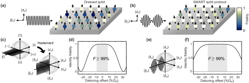
Figure 1: A qubit ensemble driven collectively by a global field consisting of (a) a continuous drive and (b) a sinusoidal modulated field. The Bloch spheres for the continuous drive is shown in c) together with the transformation from the rotating to the dressed spin frame. In d) the identity operator fidelity for a range of detuning offsets is shown where the range with fidelities above $99$ $\%$ has been shaded. The Bloch sphere and the identity operator fidelities for the sinusoidal modulated case is given in e) and f). Here $\Omega_{\text{R}}=1$ MHz.

Here, $\sigma_{x}$ and $\sigma_{z}$ are Pauli matrices acting on the qubit state and $h$ is the Planck constant. The qubit Larmor frequency $\nu(t)$ has a time dependence that is controllable by external fields, and will be used to tune the resonance between the qubit and the driving field frequency ${f}_{\text{mw}}$ for controlled qubit rotations. The maximum amplitude of the oscillatory field creates Rabi rotations of frequency $\Omega_{\text{R}}\sqrt{2}$ on the qubit. This amplitude is modulated by the $\sin{(2\pi{f}_{\text{mod}}t)}$ term, where the modulation frequency ${f}_{\text{mod}}$ is a parameter that is chosen in order to optimise the noise cancelling properties of the driving field. The factor of $\sqrt{2}$ is a scaling factor in order to compare the resulting efficiency of the driving field in the cases of dressed and SMART qubits when adopting the same root mean square power of the global field. In Fig. 1 the fidelity of an identity operation on a dressed and SMART qubit ensemble is compared for different frequency detuning offset, showing higher robustness to resonance frequency variability for the latter.

The mathematical description and computer simulation of the qubit dynamics are significantly simplified when the Hamiltonian is written in the rotating frame that precesses with the same frequency as the driving field ${f}_{\text{mw}}$. In this case,

$$H_{\text{rot}}^{\text{sin}}=\frac{h}{2}\left(\Delta\nu(t)\sigma_{z}+\Omega_{\text{R}}\sqrt{2}\sin{(2\pi{f}_{\text{mod}}t)}\sigma_{x}\right),$$ (3)

where $\Delta\nu(t)=\nu(t)-{f}_{\text{mw}}$ is the detuning between the controllable Rabi frequency and the driving field.

Dressed qubit logical states are then the $|+\rangle$ and $|-\rangle$ states in the rotating frame, that is, the states parallel and anti-parallel to the $x$ axis in a rotating frame. We highlight this fact by referring to a dressed basis, which is simply a Hadamard transformation over the rotating frame basis described in Eq. 3. This returns the logical qubit states to the conventional $z$ axis. Operating in the dressed basis implies the following axes transformations from the rotating frame basis: $|\uparrow\rangle\rightarrow|x_{\rho}\rangle$, $|\downarrow\rangle\rightarrow|\bar{x}_{\rho}\rangle$, $|+\rangle\rightarrow|z_{\rho}\rangle$, $|-\rangle\rightarrow|\bar{z}_{\rho}\rangle$, $|i\rangle\rightarrow|\bar{y}_{\rho}\rangle$ and $|\bar{i}\rangle\rightarrow|y_{\rho}\rangle$, hence a rotation about the $x$-axis in the dressed basis is equivalent to a rotation about the $z$-axis in the rotating basis etc. This change of quantisation axis can be seen from the Bloch sphere in Fig. 1(c) where the qubit states along the conventional quantisation axis $|\uparrow\rangle$ and $|\downarrow\rangle$ now are in the equatorial plane.

The Hamiltonian in the dressed basis reads

$$H_{\rho}^{\text{sin}}=\frac{h}{2}\left(\Omega_{\text{R}}\sqrt{2}\sin(2\pi{f}_{\text{mod}}t)\sigma_{z}+\Delta\nu(t)\sigma_{x}\right).$$ (4)

In general, the amplitude and frequency of the modulated global field determine its noise-cancelling properties. This example of a sinusoidal modulated global field can be extended to more sophisticated combinations of modulation components in order to cancel multiple types of noise as well.

To understand why a SMART qubit can be superior to a dressed qubit in terms of coherence time and gate performance, we derive an analytical expression for a model of quasi-static noise using the Magnus expansion series and analyse the noise cancelling properties using the geometric formalism from Ref. Zeng et al., 2019. The geometric formalism is based on a description of the time evolution of the qubit $U(t)$ in terms of a three dimensional trajectory $\vec{s}(t)$ extracted from the first term in the Magnus expansion series. This trajectory is directly related to the microwave amplitude modulation $\Omega(t)$ through its curvature $\kappa$ ($\Omega(t)=\kappa(t)$). This is explained in more detail in Appendix A.

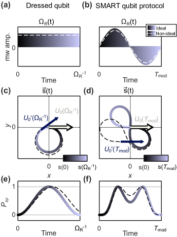
Figure 2: Geometric formalism describing noise-cancelling properties. (a-b) Global field amplitude modulation $\Omega(t)$ and (c-d) the corresponding space curve $\vec{s}(t)$, for the dressed and SMART qubit. The ideal modulation condition is plotted with a solid black line and a non-ideal condition with a dashed black line. The slope of the space curve at the end-point for the ideal (beige) and non-ideal case (blue) is plotted in (c-d) together with a black arrow representing the slope at the starting point. The evolution of a qubit initialised to $|\bar{x}_{\rho}\rangle$ is shown in (e-f).

In Fig. 2(a-d) $\Omega(t)$ and $\vec{s}(t)$ are shown in the cases of dressed and SMART qubits. Both cases show a closed space curve (solid black line), a circle for the dressed case and a figure eight for the SMART case. This indicates cancellation of first order noise. The dashed lines in Fig. 2(a,b) show examples where the amplitude is offset by some form of noise (such as fluctuation in source power) for the same gate time, resulting in a non-closed space curve or equivalently only partial first order noise cancellation. Information about the single-qubit gate can be found in the slope of $\vec{s}(T)$ at $t=0$ relative to $t=T$. Parallel slopes correspond to the identity operator and perpendicular slopes correspond to $\sqrt{\text{X}}$ and $\sqrt{\text{Y}}$ gates etc.

The geometric requirement for first order noise to cancel – that $\vec{s}(t)$ is a closed curve ($\vec{s}(0)=\vec{s}(T)$) – is achieved for the SMART qubit in Fig. 2(b,d) by synchronising the modulation frequency $f_{\rm mod}$ in a certain proportion to the Rabi frequency $\Omega_{\text{R}}$. In order for second order noise to cancel as well, the area projected from the trajectory $\vec{s}(t)$ onto the $xy$-, $xz$- and $yz$-plane must all equal zero. The sign of a projected area is determined by the winding direction of the trajectory. Hence, the figure eight trajectory followed by the SMART qubit in Fig. 2(d) has a positively signed lobe in the fourth quadrant and a negatively signed lobe in the second quadrant. The projected areas therefore sum to zero for the SMART qubits, but not for the dressed qubits. This higher order of noise cancellation translates into an improved tolerance to noise amplitudes in the case of SMART qubits, while the dressed qubit only provides first order noise cancellation.

Note that what we refer here as quasi-static noise could be originated in the stochastic electromagnetic fields of the quantum processor, but it may also have its origin in other non-idealities, such as crosstalk between qubits, fabrication variability and small unaccounted Hamiltonian terms (such as long-range dipolar coupling between spins or cross-Kerr interactions in superconducting qubits coupled through a bus cavity).

We mathematically find the optimal modulation conditions for the global field by forcing the first and second order Magnus expansion series terms to zero Zeng et al. (2019). The optimal modulation frequency $f^{\text{opt}}_{\text{mod}}$ is found to have the following relation with $\Omega_{\text{R}}$

$$f^{\text{opt}}_{\text{mod}}=\Omega_{\text{R}}\sqrt{2}/{j_{i}},$$ (5)

where $j_{i}$ is the $i$-th root of the Bessel function of zeroth order and $j_{1}=2.404826$. The derivation of this relationship can be found in Appendix A. The duration of one period of the global field is denoted $T_{\text{mod}}$. For a SMART qubit initialised in the plane perpendicular to the global field axis, driven at $f^{\text{opt}}_{\text{mod}}$ with amplitude $\Omega_{\text{R}}\sqrt{2}$ and $\Delta\nu(t)=0$, a positive rotation of $\sim 3\pi/2$ followed by a negative rotation of the same angle occur for every $T_{\text{mod}}$ of the global drive. The dressed qubit, on the other hand, continuously rotates without change in angular velocity. This is shown in Fig. 2(e,f). The back-and-forth rocking of the SMART qubit and the continuous rotation of the dressed qubit about the global field axis both contribute to the continuous echoing of low frequency noise in these encoding strategies.

IV SMART qubit two-axes control

Rotations using the SMART protocol in the dressed basis are achieved by applying frequency detuning $\Delta\nu(t)$ to the qubit with sinusoidal modulation at certain frequency and phase. The global field is always on, providing dynamically protected gates.

Detuning of individual qubits can be implemented, for example, by pulsing the gate electrode above a spin qubit in semiconductors with spin-orbit coupling, effectively shifting the gyromagnetic ratio Laucht et al. (2015); Kane (1998); by modulating

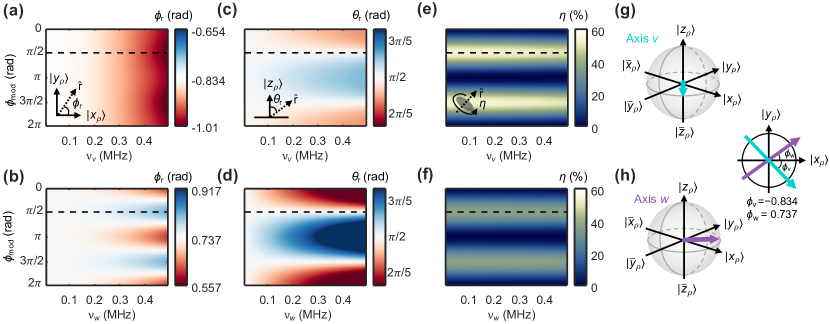
Figure 3: Rotation axis parameters (a) $\phi_{r}$ and (b) $\theta_{r}$ for axis $v$ (top) and $w$ (bottom) of the SMART qubit for different values of the control amplitude $\nu_{v,w}$ and the phase offset between the microwave and the gate modulation $\phi_{\text{mod}}$. Phase $\pi/2$ has been indicated with a dashed horizontal line. The rotation efficiency $\eta$ calculated according to Eq. 9 is shown in (c) with the maximum values of 53.9 % and 37.3 % for axis $v$ and $w$, respectively. For small values of $\nu_{v,w}$ and $\phi_{\text{mod}}=\pi/2$ the resulting pair of perpendicular axes of rotation are illustrated on Bloch spheres in (g-h) with a relative angle of $\phi_{v}=0.834$ radians to the dressed $xy$ axis system. Here $\Omega_{\text{R}}=1$ MHz.

the hyperfine coupling between an electron and the static spin of the nucleus  Laucht et al. (2015); Thiele et al. (2014); Sigillito et al. (2017); by locally changing the magnetic flux in a Josephson junction Krantz et al. (2019); and so on.

Controlled rotations about one axis $v$ using sinusoidal local detuning of the qubit are described in the dressed basis by the Hamiltonian

$$\begin{split}H_{\rho}^{v}&=H_{\text{global}}+H_{\text{local}}\\ &=H_{\text{global}}+\frac{h}{2}(\nu_{v}\sin(2\pi{f}_{\text{mod}}t+\phi_{\text{mod}})\sigma_{x}).\end{split}$$ (6)

The first term $H_{\text{global}}$ is the global field with sinusoidal modulations $\frac{h}{2}\Omega_{\text{R}}\sqrt{2}\sin(2\pi{f}_{\text{mod}}t)\sigma_{z}$ from Eq. 4. Now we add a local control term $H_{\text{local}}$ that will be responsible for addressing an individual qubit by modulating its Larmor frequency, where $\phi_{\text{mod}}$ is the phase offset between the microwave and the qubit Larmor frequency modulation and $\nu_{v}$ the detuning amplitude of the local control term. Note that specifying that the modulation frequency of the local control field is equal to the one of the global field determines the direction for this rotation axis $v$, which in principle is not one of the Cartesian axes defined before.

For two-axis control a second rotation axis $w$ can be found with a Hamiltonian of the same form as $H_{\rho}^{v}$ but with the detuning modulated at twice the frequency

$$\begin{split}H_{\rho}^{w}=H_{\text{global}}+\frac{h}{2}\left(\nu_{w}\sin(4\pi{f}_{\text{mod}}t+\phi_{\text{mod}})\sigma_{x}\right).\end{split}$$ (7)

Any other combination of odd and even harmonics would also achieve two axes control, as long as the modulation remains synchronised with the global field echoing condition. However, higher harmonics exhibit lower rotation efficiency (see filter function formalism in Appendix A). The direction of $w$ is, again, not correlated to the Cartesian directions in the general case.

The effective rotation is calculated from the time-evolution operator

$$\begin{split}U_{r}(\chi)&=\cos\left(\frac{\chi}{2}\right)\mathrm{I}-i\sin\left(\frac{\chi}{2}\right)(r_{x}\sigma_{x}+r_{y}\sigma_{y}+r_{z}\sigma_{z}),\end{split}$$ (8)

using the identities $\theta_{r}=\arctan(r_{y}/r_{x})$ and $\phi_{r}=\arctan(r_{z}(r_{x}^{2}+r_{y}^{2})^{-1/2})$, where $\hat{r}=[r_{x},r_{y},r_{z}]$ is the unit rotation vector. The rotation angle $\chi$ can be calculated from the identity component of the operator, and $\hat{r}$ reconstructed when the identity component has been subtracted. In Fig. 3 $\phi_{r}$, $\theta_{r}$ and the rotation efficiency $\eta$ is given as a function of $\phi_{\text{mod}}$ and $\nu_{v,w}$ for axes $v$ and $w$. The rotation efficiency is calculated for sinusoidal control terms according to

$$\eta_{v,w}=\frac{P_{\text{out}}}{P_{\text{in}}}=100\,\%\times\bigg{(}\frac{\chi_{v,w}^{2}}{\big{(}2\pi T_{\text{mod}}\big{)}^{2}\big{(}\frac{\nu_{v,w}}{\sqrt{2}}\big{)}^{2}}\bigg{)},$$ (9)

where $P_{\text{out}}$ is given by the squared angular velocity and the sum represents the root mean square of the control sinusoids of amplitude $\nu_{v,w}$. The rotation efficiency is $100\%$ for square pulse control of an undressed qubit and $50\%$ for frequency modulation resonance control of a dressed qubit  Laucht et al. (2017); Seedhouse et al. (2021). This shows that both $v$ and $w$ rotations have comparable control strength to the dressed qubit.

By choosing appropriate values for $\nu_{v,w}$ and $\phi_{\text{mod}}$, the two axes $v$ and $w$ can be made perpendicular. These values correspond to $\nu_{v,w}\ll\Omega_{\text{R}}$ and $\phi_{\text{mod}}=\pi/2$, giving $\phi_{w}-\phi_{v}\approx\pi/2$ and $\theta_{v,w}\approx\pi/2$, as shown in Fig. 3(g,h). Hence, we have constructed two-axes control by tailoring the amplitude and phase of two sinusoidal driving fields of frequency $f_{\text{mod}}$ and $2f_{\text{mod}}$. By combining the two driving field in a weighted sum arbitrary two-axes control, including Cartesian $xy$-axes, can be engineered as discussed in the following paragraph.

From now on we will assume $\phi_{\text{mod}}=\pi/2$ and replace the sine from the local control term in Eq. 6 and Eq. 7 with a cosine. The condition on $\nu_{v,w}$ and $\phi_{\text{mod}}$ from Fig. 3 only guarantees that the two rotation axes $v$ and $w$ are perpendicular, they do not coincide with $|x_{\rho}\rangle$ and $|y_{\rho}\rangle$ on the Bloch sphere in Fig. 3(g,h). Instead, they are rotated $-0.834$ radians ($-47.8$ degrees) in relation to the Cartesian axes. For the sake of completeness, we show that, in order to produce actual $x$- and $y$-rotations, the control terms of $v$ and $w$ can be combined in a linear fashion

$$\begin{split}H^{x,y}_{\rho}=H_{\text{global}}+\frac{h}{2}\bigg{(}\nu_{v}^{x,y}\big{(}\cos(2\pi{f}_{\text{mod}}t)-1\big{)}+\\ \nu_{w}^{x,y}\big{(}\cos(4\pi{f}_{\text{mod}}t)-1\big{)}\bigg{)}\sigma_{x}.\end{split}$$ (10)

Here, additional $-1$ terms are added in order to force the control amplitude to start and end at zero, which is advantageous for experimental reasons as the control fields are limited by a finite rise time and power. In order to find the optimal values for $\nu_{v}$ and $\nu_{w}$, GRAPE is applied Khaneja et al. (2005); Yang et al. (2019).

Table 1: Coefficients used to construct $\sqrt{\rm{X}}$ and $\sqrt{\rm{Y}}$ gates with Eq. 10 for different duration and $\Omega_{\rm{R}}=1\,\text{MHz}$.

$\sqrt{\rm{X}}$		$\sqrt{\rm{Y}}$
$\nu^{x}_{v}$ (MHz)	$\nu^{x}_{w}$ (MHz)	$\nu^{y}_{v}$ (MHz)	$\nu^{y}_{w}$ (MHz)	$t$ ($T_{\rm{mod}})$
0.1515	0.3336	-0.2154	0.2224	1
0.0893	0.1579	-0.1056	0.1136	2
0.0620	0.0921	-0.0701	0.0760	3
0.0271	0.0366	-0.0300	0.0327	7
0.0190	0.0254	-0.0210	0.0229	10

The duration of a one-qubit gate using the SMART protocol must equal a multiple $n$ of $T_{\text{mod}}$. For every $n$, the optimal values of $\nu_{v}$ and $\nu_{w}$ can be found from GRAPE. That is, each gate can be made to last for any integer number of $T_{\text{mod}}$. This is convenient as different systems can be limited by, for example, Larmor frequency tunability range or coherence times, in which case one would need longer or shorter gate duration, respectively. In Table 1, values of $\nu_{v}$ and $\nu_{w}$ are given for a range of $n$. The same data multiplied by the gate duration is plotted in Fig. 4(a,b), where the values clearly converge at longer gate duration.

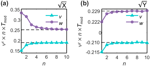
Figure 4: Coefficients $\nu_{v}$ and $\nu_{w}$ times the duration of a gate for (a) $\sqrt{\text{X}}$ and (b) $\sqrt{\text{Y}}$ gates for different gate duration according to Table 1. The dashed horizontal line indicates the convergence value. Note that in (b) the $y$-axis is discontinuous.

This convergence comes from the rotating wave approximation (RWA), where for large driving amplitudes (corresponding to short times in Fig. 4) the approximation breaks down Laucht et al. (2016). There is a compromise between accurate rotation axes and fast control, as choosing a small integer number $n$ for the gate duration forces $\nu_{v}$ and $\nu_{w}$ to be higher in order to achieve the same rotation angle, affecting the accuracy of the rotation axis angles $\theta_{r}$ and $\phi_{r}$ found from Fig. 3. The fastest possible gate is limited by the amplitude of the Larmor frequency controllability in the system.

It turns out that by modulating the global field with a cosine instead of a sine according to

$$H_{\rho}^{\text{cos}}=\frac{h}{2}(\Omega_{\text{R}}\sqrt{2}\cos(2\pi{f}_{\text{mod}}t)\sigma_{z}+\Delta\nu(t)\sigma_{x}),$$ (11)

$x$- and $y$-rotations can be achieved by simply single harmonic control terms without having to combine several harmonics in a linear fashion with coefficient extracted with GRAPE. However, the method developed here is useful for finding optimal parameters for arbitrary gate control strategies. The global microwave modulation and the Stark shift modulation for $x$-, $y$-, $v$- and $w$-rotation is shown in Fig. 5 for the dressed and SMART qubit.

V SMART qubit protocol gate fidelities

In order to assess gate robustness to frequency detuning and microwave amplitude fluctuations using the SMART protocol, a noise analysis is carried out. Our noise model is a quasi-static Gaussian noise implemented in the system Hamiltonian as follows

$$H_{\rho}=(1+\delta_{\Omega})\Omega_{\text{R}}\sqrt{2}\sin{(2\pi{f}_{\text{mod}}t)}\sigma_{z}+(\Delta\nu(t)+\delta_{\nu})\sigma_{x}.$$ (12)

Here, $\delta_{\Omega}$ and $\delta_{\nu}$ represent the amplitude and detuning offset caused by the noise, respectively. The frequency detuning noise is considered as a simple offset, while the amplitude noise is taken to be proportional to the amplitude of the driving field.

In Fig. 6(a-b) the fidelity of an identity gate is given for the bare (undressed) and the dressed qubit. A dressed $\sqrt{\text{X}}$ is shown in (c). The SMART qubit identity, $\sqrt{\text{X}}$ and $\sqrt{\text{Y}}$ gate is presented in (d-f). The first row shows fidelities corresponding to an operation generated by one fixed value of the offsets $\delta_{\Omega}$ and $\delta_{\nu}$, which represents one realisation of the noise. In the second and third rows, Gaussian averaging over several realisations has been applied, and it is shown in linear and logarithmic scales,

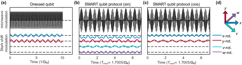
Figure 5: Global microwave field modulation and Stark shift control terms for (a) continuous drive $\sqrt{\text{X}}$ and $\sqrt{\text{Y}}$ gate and (b,c) SMART qubit $\sqrt{\text{V}}$, $\sqrt{\text{W}}$, $\sqrt{\text{X}}$ and $\sqrt{\text{Y}}$ gates. The gate durations are $10/\Omega_{\text{R}}$ for the dressed case and $7\times T_{\text{mod}}$ for the SMART case, and the relative microwave and Stark shift amplitude is to scale. In (d) the four axes are shown.

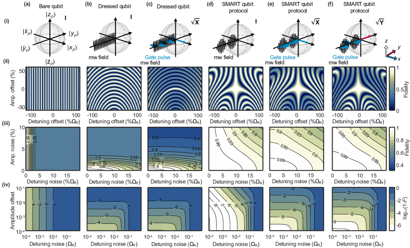
Figure 6: Gate fidelities for different values of amplitude and detuning offset/noise for the bare, dressed and SMART qubit. (a-c) show the identity gate fidelities for the bare and dressed qubit and a $\sqrt{\text{X}}$ gate for the dressed qubit, respectively. In (d-f) SMART qubit identity, $\sqrt{\text{X}}$ and $\sqrt{\text{Y}}$ is shown. Row (i) shows Bloch spheres with the relevant global field, local control field and rotation axis. In row (ii) the fidelity for offset values of amplitude and detuning is shown, and finally row (iii) and (iv) show Gaussian distributed noise in linear and log scale, respectively. Here $\Omega_{\text{R}}$ is $1$ MHz and the gate durations are according to Fig. 5. The bare qubit identity gate has the same duration as the dressed gates.

respectively. The calculated fidelity for $\pi/2$ rotations are similarly given for (d) the dressed and (e,f) the SMART qubit protocol. More details on generating the 2D noise maps and 2D noise maps for $\sqrt{\text{V}}$ and $\sqrt{\text{W}}$ are provided in Appendix B and Appendix C, respectively.

VI SMART protocol for spin qubits

We now focus on the particular example of electron spin qubits in electrostatically confined quantum dots, in which the global driving can be performed through an oscillating magnetic field or, alternatively, an oscillating electric field that couples to spins through spin-orbit coupling. This spin-orbit coupling can also be used to control locally the value of the Rabi frequency through the Stark shift of the spin resonance frequency, which is a result of the influence of gate voltage bias on the effective $g$-factor of a spin in a given quantum dot.

All our numbers are chosen in the range of spin-orbit effects found in Si/SiO₂ electrostatic quantum dots, for which abundant literature exists to inform the expected variability and degree of controllability of the interface-induced spin-orbit coupling Jones et al. (2018); Laucht et al. (2017); Veldhorst et al. (2015, 2014).

For other qubit architectures the particular physical aspects of two-qubit gates, initialisation and readout may differ significantly and the feasibility of these operations under an always-on global field needs to be assessed case-by-case.

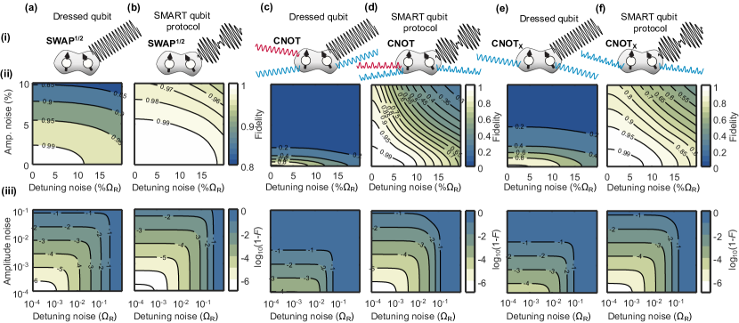
Figure 7: Two-qubit $\sqrt{\text{SWAP}}$ gate fidelities for different values of amplitude and detuning offset/noise for (a) the dressed qubit and (b) the SMART qubit. In (c) and (d) the gate fidelities for CNOT is given and in (e) and (f) for CNOT${}_{\text{X}}$. Row (i) shows two qubits with a common global field and local Stark shift fields. In Row (ii) and (iii) the gate fidelities with Gaussian noise applied are shown on a linear and log scale, respectively. Here $\Omega_{\text{R}}$ is $1$ MHz.

VI.1 Two-qubit gates

Two-qubit gates between spins based on exchange coupling can be implemented with a strategy similar to that of bare qubits. Applying voltage bias pulses to the electrostatic gates, the overlap between wavefunctions of neighbouring electrons can be tuned. In the example of bare qubits, the resulting spin-spin interaction depends on the ramp rates of the gate biases and the difference between qubit Larmor frequencies.

For the case of a driven qubit, such as the dressed or SMART qubit, the impact of the driving field on the resulting gate operation is also set by the exchange control ramp rates. The difference is that the relevant time scale is determined by the difference between Larmor and Rabi frequencies of the qubits. Further detail on the onset of the different operations for various ramp rates can be obtained in Ref. Seedhouse et al., 2021 in the case of dressed qubits.

Fidelity maps for the two-qubit gates $\sqrt{\text{SWAP}}$, CNOT and $\text{CNOT}_{\text{X}}$ are given in Fig. 7. The $\sqrt{\text{SWAP}}$ gate is implemented assuming exchange gate control, where SWAP-like operation is the native two-qubit gate for qubits having the same resonance frequency Seedhouse et al. (2021). The meaning of $\text{CNOT}_{\text{X}}$ here is a NOT operation on the target qubit conditional on the control qubit being $|x\rangle$ or $|\bar{x}\rangle$ instead of $|0\rangle$ or $|1\rangle$. The CNOT and $\text{CNOT}_{\text{X}}$ gate sequences used here are $(\sqrt{{\text{Y}}}^{\dagger}\otimes\text{I})\sqrt{\text{SWAP}}(\sqrt{{\text{X}}}^{\dagger}\otimes\sqrt{\text{X}})\sqrt{\text{SWAP}}(\sqrt{\text{Y}}\otimes\text{I})$ and $\sqrt{\text{SWAP}}(\sqrt{\text{X}}^{\dagger}\otimes\sqrt{\text{X}})\sqrt{\text{SWAP}}$. Here the assumption that the two qubits experience the same noise level is made (see Appendix B for more details). For both one- and two-qubit gates the robustness to detuning and amplitude noise is seen to improve significantly compared to the bare and dressed case.

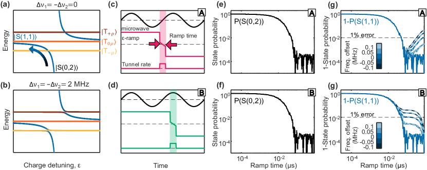
Figure 8: SMART two-qubit initialisation and readout. a) Energy diagram of the SMART two-qubit system for zero frequency detuning and for (b) $\Delta\nu_{1}=-\Delta\nu=0.2$ MHz. Initialisation of S(1,1) from S(0,2) with ramping centered about (c) the minimum microwave amplitude and (d) the maximum microwave amplitude of the global field. The results with different ramp rates and fixed charge detuning ramp range 50 GHz $\rightarrow$ $-50$ GHz ($\sim$0.2 meV) is shown in (e-h) where the probability of S(0,2) and S(1,1) is plotted against ramp time. Fixed offsets in frequency detuning ($\Delta\nu_{1},\Delta\nu_{2}$) are introduced, with magnitudes given by the colorbar (two-colored dashed line representing the two qubits). Parameters used here include $\Omega_{\text{R}1}=\Omega_{\text{R}2}=1$ MHz, $(\Delta\nu_{1},\Delta\nu_{2})\in\{0,\pm 0.05,\pm 0.1\}$ MHz, $t_{c}=0.5$ GHz. The total time is $2\times{T}_{\text{mod}}$.

VI.2 Initialisation and readout

High fidelity initialisation and readout are necessary for error-corrected quantum computing strategies. The constant driving field creates oscillations between the $|0\rangle$ and $|1\rangle$ states, which limit the range of strategies that can be used for initialisation and readout – strategies based on energy-dependent transitions are hard to harmonise with a driving field. Both initialisation and readout are studied here in the context of strategies leveraging the Pauli spin blockade.

Initialisation of two-qubit SMART states is done similarly to the dressed spin qubit Seedhouse et al. (2021), by ramping from negative to positive detuning at different rates. In Fig. 8(a) the energy diagram of the system as a function of charge detuning is shown at finite global field microwave amplitude with zero frequency detuning, and in (b) with $\Delta\nu_{1}=-\Delta\nu_{2}=0.2$ MHz. For non-zero frequency detuning, an anticrossing appears and the ramping rate determines whether or not the spin crosses this energy gap diabatically. The system is initialised to an S(1,1) state from a S(0,2) state with a ramp centered about either (c) the minimum or (d) the maximum microwave amplitude (A and B). The transition from positive to negative detuning consists of a step before and after the slow ramp to achieve lower ramp rate, as seen from $\varepsilon$-ramp in Fig. 8(c,d). The state probability of S(0,2) and S(1,1) is given for different ramp times in Fig. 8(e-h) for the two cases. For comparison two-qubit dressed initialisation is shown in Fig. 9. To show the robustness to resonance frequency variability different combinations of $\Delta\nu_{1}$ and $\Delta\nu_{2}$ $\in\{0,\pm 0.05,\pm 0.1\}$ MHz are simulated. A S(1,1) state is achieved with $>99$ $\%$ fidelity after approximately 0.1 µs for case A and 1 µs for case B (at worst-case frequency offset). Centering the ramp about the minimum microwave amplitude (A) looks to be a more robust options causing less mixing with the triplet states. This can be explained by looking at the effective echoing as a result of the global field after the ramp. For case A close to a full period of the global field follows the ramp, whereas for case B less than three quarters of a period.

Readout can be performed similarly by reversing the process described above and relying on Pauli Spin blockade in the dressed frame Seedhouse et al. (2021). In that case, the spin blockade is guaranteed for the duration of the spin relaxation time, and readout can be performed using some charge sensing technique. Note, however, that both the spin relaxation time and the charge readout bandwidth can be impacted by the field of the global driving, which can impose some engineering challenges. Further discussions on the engineering aspects of globally driven spin architecture are out of the scope of the present work, and some initial results in this direction can be seen in Refs. Vahapoglu et al. (2021a) and  Vahapoglu et al. (2021b).

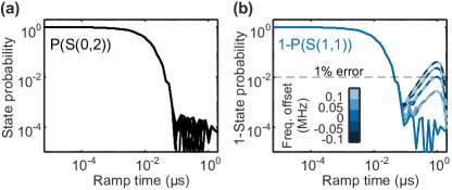
Figure 9: Dressed two-qubit initialisation for different ramp times and frequency detuning offsets. The state probability of S(0,2) and S(1,1) is shown with $\Omega_{\text{R}}=1$ MHz and the total time $2/\Omega_{\text{R}}$.

VII Summary

In this paper we propose to combine pulse engineering with electromagnetic dressing of qubits, in what we denote the SMART protocol. We have shown that qubits can be made more robust to detuning and amplitude variability caused by noise and/or sample inhomogeneity by applying a sinusoidal modulation to the global field, cancelling both first and second order noise terms in a Magnus expansion. By applying more complex modulation such as multi-tone driving, higher order noise terms can be cancelled as well. This is left for future work. We have analysed two-qubit gates, initialisation and readout in the particular example of spin qubits in quantum dots, however the SMART protocol can be applied to other systems with global coherent driving. The SMART protocol provides a clear and scalable path in terms of engineering constraints, making it a potential strategy for large-scale quantum computing.

Appendix A Magnus expansion series

In order to investigate how certain noise effects our system we look at the Hamiltonian in the interaction picture, found by transforming the noise Hamiltonian ($\delta\beta\sigma_{i}$) with the time evolution operator from the noiseless driving Hamiltonian $U(t)$. Here $\delta\beta$ is the fluctuation parameter on axis $i$ approximated as a constant for slow noise

$$H_{I}(t)=U(t)^{\dagger}\sigma_{i}U(t)\delta\beta.$$ (13)

The time evolution operator in the interaction picture is given by

$$U_{I}(t)=\exp\left(\sum_{i=1}^{\infty}{A_{i}(t)}\right),$$ (14)

and should equal identity for perfect noise cancellation. By truncating the sum we can find solutions where certain orders of noise cancels. For example, by making sure $A_{1}(T)$ is zero first order noise cancels out etc.

The first two order of the expansion of $U_{I}(t)$ include

$$A_{1}(t)=\frac{1}{\delta\beta}\int_{0}^{t}{H_{\text{I}}(t_{1})dt_{1}},$$ (15)

$$A_{2}(t)=\frac{1}{2\delta\beta^{2}}\int_{0}^{t}{dt_{1}}\int_{0}^{t_{1}}{dt_{2}[H_{\text{I}}(t_{1}),H_{\text{I}}(t_{2})]}.$$ (16)

The space curve parametrisation in Fig. 2(b) is given by

$$\vec{s}(t)=(x(t),y(t),z(t)),$$ (17)

where $x(t),y(t),z(t)$ is extracted from $A_{1}(t)$ according to

$$A_{1}(t)=x(t)\sigma_{x}+y(t)\sigma_{y}+z(t)\sigma_{z}.$$ (18)

The deduction of Eq. 5 follows here corresponding to first and second order noise cancellation by forcing Eq. 15 to zero. We can write Eq. 15 in the form of a supermatrix $\hat{U}(t)$ using the identity $\text{vec}(ABC)=C^{T}\otimes{A}\hskip 2.84544pt\text{vec}(B)$ to allow for arbitrary noise axis

$$\text{vec}(A_{1i}(t))=\frac{1}{\delta\beta}\int_{0}^{t}{U^{T}(t_{1})\otimes U^{\dagger}(t_{1})\delta\beta dt_{1}}\hskip 2.84544pt\text{vec}(\sigma_{i}).$$ (19)

An arbitrary driving field $\Omega(t)$ about axis $\sigma_{z}$ (chosen to simplify maths, also dressed basis $x$-axis) gives us the time evolution operator

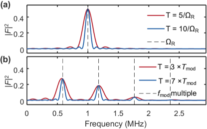
Figure 10: Filter function formalism applied to (a) the dressed and (b) the SMART qubit showing noise frequency susceptibility and equivalently controllability. Here $\Omega_{\text{R}}=1$ MHz.

$$U(t)=\text{diag}(\exp\bigg{\{}-i\pi\int_{0}^{t}{\Omega(t)dt}\bigg{\}},\exp\bigg{\{}i\pi\int_{0}^{t}{\Omega(t)dt}\bigg{\}}),$$ (20)

and the corresponding supermatrix

$$\hat{U}(t)=\text{diag}(1,\exp\bigg{\{}-2i\pi\int_{0}^{t}{\Omega(t)dt}\bigg{\}},\exp\bigg{\{}2i\pi\int_{0}^{t}{\Omega(t)dt}\bigg{\}},1).$$ (21)

Now looking at detuning noise in the dressed basis we find

$$A_{1x}(t)=\text{mat}\bigg{(}\frac{1}{\delta\beta}\int_{0}^{t}{\Omega(t)\hat{U}(t)\delta\beta{dt}\hskip 2.84544pt\text{vec}(\sigma_{x})}\bigg{)}$$ (22)

For $A_{1x}(t)$ to be zero we have the following condition

$$\int_{0}^{T}{\exp\bigg{\{}\pm 2i\pi\int_{0}^{t}{\Omega(t_{1})dt_{1}}\bigg{\}}dt}=0.$$ (23)

Choosing a sine wave control with one period duration we get

$$\int_{0}^{1/f}{\exp\bigg{\{}\pm 2i\pi\int_{0}^{t}{\Omega\sin(2\pi{ft_{1}})dt_{1}}\bigg{\}}dt}=0$$ (24)

$$\int_{0}^{1/f}{\exp\bigg{\{}\mp{i}\frac{\Omega}{f}\cos(2\pi{ft})\bigg{\}}dt}=0$$ (25)

This can be recognised as one of Bessel’s integrals with solution $\Omega/f=j_{i}$, where $j_{i}$ is the $i$-th root. It can be seen that $A_{1}$ is zero for $T=\frac{n}{2f}$. The second order term $A_{2}$ goes to zero when the time is chosen appropriately, which is $\frac{n}{f}$ in this case with any integer $n$. This is because the chosen control is a periodic and odd function, meaning that the second order cancellation happens for any values of $\Omega/f$ as long as the duration is a multiple of the period. This corresponds to $n$ loops through the space curve in Fig. 2(d).

By substituting the fluctuation parameter with a tone of variable frequency ($\underline{\delta\beta}(f,t)=\delta\beta\exp(-2i\pi{f}t)$) we can probe the noise susceptibility of the SMART qubit at different frequencies (or similarly the controllability at certain control frequencies), according to filter function formalism. This is shown in Fig. 10.

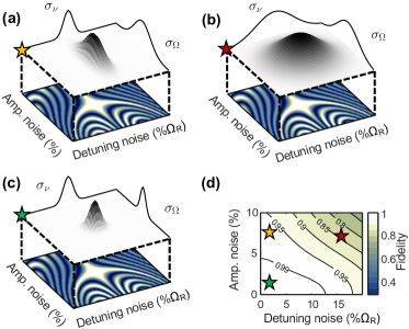
Figure 11: Schematic of method used to construct Gaussian noise model. The fixed offset noise map is multiplied by 2D Gaussians with $\sigma_{x}$ and $\sigma_{y}$ corresponding to the detuning and amplitude noise levels, shown here for three different cases (a-c). The stars in (d) indicate the following: low detuning noise and high amplitude noise (yellow), high detuning noise and high amplitude noise (red) and low amplitude noise and low detuning noise (green).

Appendix B Simulation details of 2D noise maps

For the 2D noise maps in Fig. 6 and Fig. 7 the Hamiltonian given in Eq. 12 is used. In order to generate the maps the following steps are executed:

1. Construct time-dependent Hamiltonian, $H$ with certain detuning and amplitude offset $(\delta_{\nu},\delta_{\Omega})$ according to Eq. 12.

2. Time-evolve $H$ into time-evolution operator $U$ at a certain time.

3. Calculate the fidelity of the resulting operator $U$ by looking at the overlap with the target operator.

4. Repeat the steps above for different amplitude and detuning offset values to create a 2D fidelity map $F(\delta_{\nu},\delta_{\Omega})$.

5. Apply Gaussian averaging across the fixed noise map generated above, where the width of the applied Gaussian distribution is set by the noise level. That is, multiply the fixed noise map by a normalised 2D Gaussian around zero offset with widths ($\sigma_{\nu},\sigma_{\Omega}$) given by the noise levels (See Fig. 11).

For the two-qubit case the noise levels of the two qubits are assumed to be the same. The same procedure as for the one-qubit gates is then followed, but integrating over all four noise dimensions $(\delta_{\nu{1}},\delta_{\nu{2}},\delta_{\Omega{1}},\delta_{\Omega{2}})$. Note that we assume there is no noise on the exchange coupling for the simulation.

Appendix C 2D noise maps for axis v and w

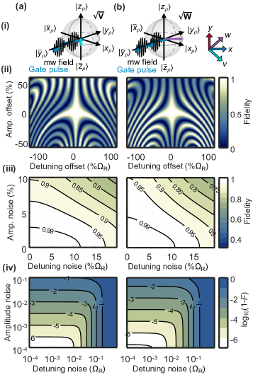
Figure 12: Gate fidelity maps for (a) the $\sqrt{{\text{V}}}$ gate and (b) the $\sqrt{{\text{W}}}$ gate. Row (i) shows Bloch spheres with the relevant global field, local control field and rotation axis. In row (ii) the fidelity for offset values of amplitude and detuning is shown, and finally row (iii) and (iv) show Gaussian distributed noise in linear and log scale, respectively.

The 2D noise maps of $\pi/2$ rotation about the ${v}$ and ${w}$ axes in Fig. 12 are found to be similar to the SMART $\sqrt{\text{X}}$ and $\sqrt{\text{Y}}$ gates.

References

- Knill (2005) E. Knill, Nature 434, 39 (2005).
- Fowler et al. (2012) A. G. Fowler, M. Mariantoni, J. M. Martinis, and A. N. Cleland, Physical Review A 86, 032324 (2012).
- Muhonen et al. (2015) J. T. Muhonen, A. Laucht, S. Simmons, J. P. Dehollain, R. Kalra, F. E. Hudson, S. Freer, K. M. Itoh, D. N. Jamieson, J. C. McCallum, A. S. Dzurak, and A. Morello, Journal of Physics: Condensed Matter 27, 154205 (2015).
- Watson et al. (2018) T. F. Watson, S. G. J. Philips, E. Kawakami, D. R. Ward, P. Scarlino, M. Veldhorst, D. E. Savage, M. G. Lagally, M. Friesen, S. N. Coppersmith, M. A. Eriksson, and L. M. K. Vandersypen, Nature 555, 633 (2018).
- Yoneda et al. (2018) J. Yoneda, K. Takeda, T. Otsuka, T. Nakajima, M. R. Delbecq, G. Allison, T. Honda, T. Kodera, S. Oda, Y. Hoshi, N. Usami, K. M. Itoh, and S. Tarucha, Nature Nanotechnology 13, 102 (2018).
- Yang et al. (2019) C. H. Yang, K. W. Chan, R. Harper, W. Huang, T. Evans, J. C. C. Hwang, B. Hensen, A. Laucht, T. Tanttu, F. E. Hudson, S. T. Flammia, K. M. Itoh, A. Morello, S. D. Bartlett, and A. S. Dzurak, Nature Electronics 2, 151 (2019).
- Harty et al. (2014) T. P. Harty, D. T. C. Allcock, C. J. Ballance, L. Guidoni, H. A. Janacek, N. M. Linke, D. N. Stacey, and D. M. Lucas, Physical Review Letters 113, 220501 (2014).
- Chow et al. (2009) J. M. Chow, J. M. Gambetta, L. Tornberg, J. Koch, L. S. Bishop, A. A. Houck, B. R. Johnson, L. Frunzio, S. M. Girvin, and R. J. Schoelkopf, Physical Review Letters 102, 090502 (2009).
- Rong et al. (2015) X. Rong, J. Geng, F. Shi, Y. Liu, K. Xu, W. Ma, F. Kong, Z. Jiang, Y. Wu, and J. Du, Nature Communications 6, 8748 (2015).
- Barends et al. (2014) R. Barends, J. Kelly, A. Megrant, A. Veitia, D. Sank, E. Jeffrey, T. C. White, J. Mutus, A. G. Fowler, B. Campbell, Y. Chen, Z. Chen, B. Chiaro, A. Dunsworth, C. Neill, P. O’Malley, P. Roushan, A. Vainsencher, J. Wenner, A. N. Korotkov, A. N. Cleland, and J. M. Martinis, Nature 508, 500 (2014).
- Timoney et al. (2011) N. Timoney, I. Baumgart, M. Johanning, A. F. Varón, M. B. Plenio, A. Retzker, and C. Wunderlich, Nature 476, 185 (2011).
- Laucht et al. (2017) A. Laucht, R. Kalra, S. Simmons, J. P. Dehollain, J. T. Muhonen, F. A. Mohiyaddin, S. Freer, F. E. Hudson, K. M. Itoh, D. N. Jamieson, J. C. McCallum, A. S. Dzurak, and A. Morello, Nature Nanotechnology 12, 61 (2017).
- Wu et al. (2019) S.-H. Wu, M. Amezcua, and H. Wang, Physical Review A 99, 063812 (2019).
- Cai et al. (2012) J.-M. Cai, F. Jelezko, N. Katz, A. Retzker, and M. Plenio, New Journal of Physics 14, 093030 (2012).
- Kane (1998) B. E. Kane, Nature 393, 133 (1998).
- Veldhorst et al. (2017) M. Veldhorst, H. G. J. Eenink, C. H. Yang, and A. S. Dzurak, Nature Communications 8, 1766 (2017).
- Seedhouse et al. (2021) A. E. Seedhouse, I. Hansen, A. Laucht, C. H. Yang, A. S. Dzurak, and A. Saraiva, arXiv:2108.00798 [cond-mat, physics:quant-ph] (2021), arXiv:2108.00798 [cond-mat, physics:quant-ph] .
- Vahapoglu et al. (2021a) E. Vahapoglu, J. P. Slack-Smith, R. C. C. Leon, W. H. Lim, F. E. Hudson, T. Day, T. Tanttu, C. H. Yang, A. Laucht, A. S. Dzurak, and J. J. Pla, arXiv:2012.10225 [cond-mat] (2021a), arXiv:2012.10225 [cond-mat] .
- Jones et al. (2018) C. Jones, M. A. Fogarty, A. Morello, M. F. Gyure, A. S. Dzurak, and T. D. Ladd, Physical Review X 8, 021058 (2018).
- Zwanenburg et al. (2013) F. A. Zwanenburg, A. S. Dzurak, A. Morello, M. Y. Simmons, L. C. L. Hollenberg, G. Klimeck, S. Rogge, S. N. Coppersmith, and M. A. Eriksson, Reviews of Modern Physics 85, 961 (2013).
- Gonzalez-Zalba et al. (2020) M. F. Gonzalez-Zalba, S. de Franceschi, E. Charbon, T. Meunier, M. Vinet, and A. S. Dzurak, arXiv:2011.11753 [cond-mat, physics:quant-ph] (2020), arXiv:2011.11753 [cond-mat, physics:quant-ph] .
- Itoh and Watanabe (2014) K. M. Itoh and H. Watanabe, MRS Communications 4, 143 (2014).
- Hensen et al. (2020) B. Hensen, W. Wei Huang, C.-H. Yang, K. W. Chan, J. Yoneda, T. Tanttu, F. E. Hudson, A. Laucht, K. M. Itoh, T. D. Ladd, A. Morello, and A. S. Dzurak, Nature Nanotechnology 15, 13 (2020).
- Veldhorst et al. (2015) M. Veldhorst, C. H. Yang, J. C. C. Hwang, W. Huang, J. P. Dehollain, J. T. Muhonen, S. Simmons, A. Laucht, F. E. Hudson, K. M. Itoh, A. Morello, and A. S. Dzurak, Nature 526, 410 (2015).
- Ruskov et al. (2018) R. Ruskov, M. Veldhorst, A. S. Dzurak, and C. Tahan, Physical Review B 98, 245424 (2018).
- Khaneja et al. (2005) N. Khaneja, T. Reiss, C. Kehlet, T. Schulte-Herbrüggen, and S. J. Glaser, Journal of Magnetic Resonance 172, 296 (2005).
- Zeng et al. (2019) J. Zeng, C. H. Yang, A. S. Dzurak, and E. Barnes, Physical Review A 99, 052321 (2019).
- Mollow (1969) B. R. Mollow, Physical Review 188, 1969 (1969).
- Xu et al. (2007) X. Xu, B. Sun, P. R. Berman, D. G. Steel, A. S. Bracker, D. Gammon, and L. J. Sham, Science 317, 929 (2007).
- Barnes et al. (2015) E. Barnes, X. Wang, and S. Das Sarma, Scientific Reports 5, 12685 (2015).
- Laucht et al. (2015) A. Laucht, J. T. Muhonen, F. A. Mohiyaddin, R. Kalra, J. P. Dehollain, S. Freer, F. E. Hudson, M. Veldhorst, R. Rahman, G. Klimeck, K. M. Itoh, D. N. Jamieson, J. C. McCallum, A. S. Dzurak, and A. Morello, Science Advances 1, e1500022 (2015).
- Thiele et al. (2014) S. Thiele, F. Balestro, R. Ballou, S. Klyatskaya, M. Ruben, and W. Wernsdorfer, Science 344, 1135 (2014).
- Sigillito et al. (2017) A. J. Sigillito, A. M. Tyryshkin, T. Schenkel, A. A. Houck, and S. A. Lyon, Nature Nanotechnology 12, 958 (2017).
- Krantz et al. (2019) P. Krantz, M. Kjaergaard, F. Yan, T. P. Orlando, S. Gustavsson, and W. D. Oliver, Applied Physics Reviews 6, 021318 (2019).
- Laucht et al. (2016) A. Laucht, S. Simmons, R. Kalra, G. Tosi, J. P. Dehollain, J. T. Muhonen, S. Freer, F. E. Hudson, K. M. Itoh, D. N. Jamieson, J. C. McCallum, A. S. Dzurak, and A. Morello, Physical Review B 94, 161302 (2016).
- Veldhorst et al. (2014) M. Veldhorst, J. C. C. Hwang, C. H. Yang, A. W. Leenstra, B. de Ronde, J. P. Dehollain, J. T. Muhonen, F. E. Hudson, K. M. Itoh, A. Morello, and A. S. Dzurak, Nature Nanotechnology 9, 981 (2014).
- Vahapoglu et al. (2021b) E. Vahapoglu, J. P. Slack-Smith, R. C. C. Leon, W. H. Lim, F. E. Hudson, T. Day, J. D. Cifuentes, T. Tanttu, C. H. Yang, A. Saraiva, M. L. W. Thewalt, A. Laucht, A. S. Dzurak, and J. J. Pla, arXiv:2107.14622 [cond-mat] (2021b), arXiv:2107.14622 [cond-mat] .