Bite-Weight Estimation Using Commercial Ear Buds

Abstract

While automatic tracking and measuring of our physical activity is a well established domain, not only in research but also in commercial products and every-day life-style, automatic measurement of eating behavior is significantly more limited. Despite the abundance of methods and algorithms that are available in bibliography, commercial solutions are mostly limited to digital logging applications for smart-phones. One factor that limits the adoption of such solutions is that they usually require specialized hardware or sensors. Based on this, we evaluate the potential for estimating the weight of consumed food (per bite) based only on the audio signal that is captured by commercial ear buds (Samsung Galaxy Buds). Specifically, we examine a combination of features (both audio and non-audio features) and trainable estimators (linear regression, support vector regression, and neural-network based estimators) and evaluate on an in-house dataset of 8 participants and 4 food types. Results indicate good potential for this approach: our best results yield mean absolute error of less than 1 g for 3 out of 4 food types when training food-specific models, and 2.1 g when training on all food types together, both of which improve over an existing literature approach.

I Introduction

In the context of dietary monitoring, various wearable sensors have been proposed in order to measure different parameters of eating behavior. One of the first sensors that was used is the in-ear microphone: the in-ear placement enables the capturing chewing sensors clearly as they are transmitted through the skull during mastication [1].

Alternative sensors have also been studied in literature. A piezoelectric sensor has been used in [2]; the sensor is attached on the skin close to the jaw that captures muscle movement during mastication. The periodic nature of chewing is also present in the piezoelectric sensor’s signal and is used to detect chewing. Alternative placements of the piezoelectric sensor have also been examined, such as attached to smart glasses or to neck collars [3] [4]. Surface electromyography (EMG) has also been used for chewing detection [5] [6], however, is currently one of the least discrete solutions.

Sensors for estimating the weight of a meal (or bite) have also been proposed, and achieve relatively high effectiveness and low errors. However, the sensors require manual placement and activation (e.g. plate weight scale [7]) or are part of the table [8] and thus cannot be used in free-living conditions such as eating outside or on-the-go.

More recently, the interest has been shifting to off-the-shelf solutions to eliminate the need for specialized hardware as well as decrease the sensors’ intrusiveness. In particular, the 3D accelerometers and gyroscopes that are commonly embedded in commercial smart-watches can be used to ambiently detect eating gestures (i.e. the repeated movements of bringing food to the mouth from a plate, tray, etc) and achieve very promising results in challenging, free-living conditions [1] [9] [10] [11]. Alternatively, an accelerometer mounted on the temporalis [12, 13] has also been used to detect muscle contraction during mastication with promising effectiveness.

Additionally, analysis of photos taken with smart phones can provide detailed information about eating habits, including types of consumed food, ingredients, etc (for example, the goFOOD^TM [14] system can estimate the calorie and macro-nutrient content of a meal based on either two photos of the meal or a short video). A single photo is used in [15] to perform segmentation, recognition, and volume estimation of different foods, and results show similar effectiveness to methods that require multiple photos of the meal.

In this work, we propose a method for estimating bite weight using the audio signal of commercially available ear buds. Our approach includes extracting features that are used to train bite weight estimators, based on annotations of start and stop time-stamps of chews and food type. We evaluate different feature sets and different types of estimators on an in-house dataset we have collected, using leave-one-subject-out (LOSO) training and testing. We examine two cases, one where food type information is available (corresponding to a use-case where food information is obtained by asking the user directly or by some food-type recognition system such as [14]) and one where it is not (corresponding to a use-case where only chewing activity is detected using some audio-based automated method such as [16]).

II Related work

An algorithm for bite-weight estimation, also from sound captured by an in-ear microphone, has been proposed in [17]. Audio was recorded at $44$ kHz; a total of $8.64$ hours were recorded from eight individuals.

The algorithm proposed in [17] used $8$ features (Table I of [17]) that can be extracted from a sequence of chews. Of these $8$ features, $7$ can be computed solely from the start and stop time-stamps of the chews, and only $1$ requires audio signal (i.e. mean signal energy). For each chewing bite, these $8$ features are extracted $6$ times: from the entire chewing bout, from the 1st, 2nd, and 3rd third of the chewing bout, and from the chewing bouts that consist of the first $3$ and $5$ chews only, respectively. This yields $48$ features; two more features are computed and a final vector of $50$ features is produced.

A linear regression (with bias) model is used to estimate bite weight. A different model is trained for each food type (a total of three food types are used: potato chip, lettuce, and apple). Two methods of feature selection are examined: manual selection based on Spearman’s correlation coefficient (between each feature and the bite-weight) and step-wise regression fit. Authors conclude that both methods yield similar results.

In this work, we differentiate significantly from [17] by (a) using commercially available ear buds, (b) focusing on audio-based features and exploring different aggregation methods, and (c) comparing different regression models for bite weight estimation.

III Bite-weight estimation algorithm

Our proposed approach aims to estimate the weight of a single bite. In short, we first extract a set of features (we examine both non-audio and audio features) which we then use to train an estimation model. Models are trained in the typical LOSO scheme, where a different model is trained for each subject of the dataset using the data from the other subjects each time.

III-A Feature extraction

We use two distinct sets of features. The first set (non-audio features) does not depend on the audio signal, but only on the start and stop time-stamps of the chews (Figure 1). Note that in this work the start and stop time-stamps have been determined manually. Specifically, let $t_{1}[i]$ and $t_{2}[i]$ for $i=1,\ldots,n$ denote the start and stop time-stamps of a bout of $n$ chews. We compute the following six features: number of chews (i.e. $n$), mean and standard deviation of chew duration (chew duration is $t_{2}[i]-t_{1}[i]$), and mean and standard deviation of chewing rate (instantaneous chewing rate is estimated as $t_{1}[i]-t_{1}[i-1]$), and food type (as is a categorical variable).

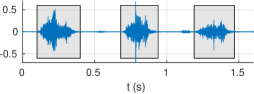
Figure 1: Example of audio signal: the first three chews of an apple bite are down, along with the manual ground-truth (gray boxes).

The second set of features is based on the audio signal. A challenge lays in the fact that (a) each chewing bout has a different duration and different number of chews, (b) each individual chew has a different duration. To overcome this, we follow a two-step process: first, one feature vector is extracted from each individual chew of a single chewing bout, and then, all the features vectors of the chews that belong to a single chewing about are aggregated together to produce a final, single feature vector for the chewing bout (this final vector is then used for training the weight predictors).

In the first step, the features that we extract from each individual chew are the ones used in [7, 18]. The features include signal energy in log-scale energy bands, higher order statistics (including skewness and kurtosis), and fractal dimension. Estimating each of those features is independent of the length of the available audio signal (i.e. from chew duration); this allows us to obtain comparable values for each feature among chews of varying duration. After extracting the features for the entire dataset we standardize them by subtracting the mean (of each feature) and dividing by its standard deviation.

In the second step, we aggregate the features vectors of the chews of each chewing bout. We examine two similar approaches to this: bag-of-words (BoW) and vectors of locally aggregated descriptors (VLAD). Centroids are obtained over the available training portion of the dataset (AIC is used for selecting the number of centroids), which are then used both on the train as well as the test portions of the dataset.

III-B Bite-weight estimators

To estimate the bite weight from the available features, we examine four different algorithms. The first estimator we evaluate is LR, similar to [17]. We have also experimented with models that include cross-product terms but have found that the overall effectiveness is not affected significantly.

The second algorithm is support vector regression (SVR). We use a radial-basis function (RBF) kernel, and use a grid search for hyper-parameters $C$ and $\gamma$ by randomly splitting the data from the $m-1$ subjects to $70\%$ for training and $30\%$ for validation. We search for $C$ in $10^{i},\,i=-2,-1,0,1,2$ and for $\gamma=10^{i}n^{-1},\,i=-1,0,1,2,3$, where $n$ is the length of the feature vector.

We also examine classic feed-forward neural networks (FFNN). We consider architectures with either $2$ or $3$ hidden layers, and $5$, $10$, $15$, and $20$ neurons per layer (thus, a total of $8$ distinct architectures, as we do not consider architectures with different number of neurons per layer). The choice of the architecture is treated as the hyper-parameter of this model and is selected based on a $90\%$ training and $10\%$ validation split of the $m-1$ subjects, and is thus different for each subject. Training minimizes the mean absolute error (MAE); learning rate is set to $0.01$ and the maximum number of epochs is $1,000$. We use the BFGS Quasi-Newton back-propagation algorithm.

Finally, we also examine generalized regression neural networks (GRNN) [19] with Gaussian kernel. Similarly to the previous models, we also select the hyper-parameter $\sigma$ of the kernel using a train-validation split on the $m-1$ subjects.

IV Dataset

To evaluate our approach we have collected an in-house dataset. A total of 8 participants were enrolled for the data collection trials ($6$ males and $2$ females, age $25\pm 1.07$ years, body-mass index $25.49\pm 3.06$). Four different food types were consumed: apple, banana, rice, and potato chips. These four types were selected as they have a unique combination of crispiness (apple and potato chips) and wetness (apple and banana). The dataset includes $2$ hours of eating and contains a total of $473$ chewing bouts and $7.539$ chews.

Audio signals were collected by using commercially available Samsung Galaxy Buds. We have created a custom Android application that captures synchronized audio (at $44.1$ kHz, $16$ bit) from the ear buds and plate weight (at $1$ Hz) from a Bluetooth-enabled plate scale. The plate weight scale has been used to derive ground truth values for bite weight. A video recording of each session has also been captured to further assist us in the annotation process.

V Evaluation

To evaluate our approach we perform various combinations of feature sets and estimation models. Given the non-audio based feature set and the two methods of aggregating the audio based features, we examine the following five combinations: non-audio features ($\mathbf{f}_{1}$), audio with BoW ($\mathbf{f}_{2}$), audio with VLAD ($\mathbf{f}_{3}$), combination of non-audio and audio with BoW features ($\mathbf{f}_{4}$), and combination of non-audio and audio with VLAD features ($\mathbf{f}_{5}$). For each of these feature sets we examine four estimators (Section III-B): LR, SVR, FFNN, GRNN. Finally, we train five different models per combination: the first four are food specific, while the fifth is trained on the data from all food types. Table I shows the mean absolute error per experiment, and Table II shows the mean absolute percentage error (%) in the same structure. All experiments are performed in LOSO fashion; thus, each result is the mean across the $8$ participants of our dataset.

TABLE I: Mean and standard deviation absolute errors per algorithm and feature set. Best result (lowest error) in red.

	Apple	Banana	Rice	Chips	All
	LR
$\mathbf{f}_{1}$	$3.02\,(2.3)$	$5.89\,(2.8)$	$3.80\,(2.5)$	$0.93\,(0.7)$	$4.94\,(3.4)$
$\mathbf{f}_{2}$	$4.13\,(3.4)$	$5.82\,(3.9)$	$3.82\,(2.2)$	$1.23\,(0.8)$	$3.70\,(3.2)$
$\mathbf{f}_{3}$	$4.83\,(3,7)$	$5.57\,(3.4)$	$5.06\,(3.2)$	$1.10\,(0.8)$	$3.86\,(3.4)$
$\mathbf{f}_{4}$	$3.65\,(2.5)$	$5.54\,(3.3)$	$3.86\,(3.1)$	$1.02\,(0.7)$	$3.24\,(2.8)$
$\mathbf{f}_{5}$	$3.15\,(2.2)$	$5.97\,(3.3)$	$3.74\,(2.7)$	$0.92\,(0.7)$	$3.44\,(3.0)$
	SVR
$\mathbf{f}_{1}$	$3.18\,(2.2)$	$6.30\,(3.2)$	$3.97\,(2.7)$	$0.97\,(0.8)$	$4.52\,(3.3)$
$\mathbf{f}_{2}$	$4.76\,(3.5)$	$5.01\,(3.2)$	$4.44\,(3.0)$	$1.17\,(0.8)$	$3.66\,(3.2)$
$\mathbf{f}_{3}$	$5.07\,(3.3)$	$5.11\,(3.2)$	$5.02\,(3.2)$	$1.12\,(0.8)$	$3.76\,(3.5)$
$\mathbf{f}_{4}$	$3.57\,(2.3)$	$5.56\,(3.2)$	$3.19\,(2.6)$	$1.05\,(0.8)$	$3.16\,(2.9)$
$\mathbf{f}_{5}$	$3.00\,(2.4)$	$5.44\,(3.4)$	$3.68\,(2.7)$	$1.00\,(0.8)$	$3.02\,(2.5)$
	FFNN
$\mathbf{f}_{1}$	$3.70\,(2.7)$	$5.17\,(3.6)$	$4.72\,(3.2)$	$0.93\,(0.8)$	$3.31\,(3.0)$
$\mathbf{f}_{2}$	$4.19\,(3.7)$	$4.68\,(3.8)$	$4.29\,(3.4)$	$1.00\,(0.9)$	$3.86\,(3.4)$
$\mathbf{f}_{3}$	$3.64\,(2.6)$	$4.10\,(3.2)$	$3.52\,(2.1)$	$0.81\,(0.6)$	$4.10\,(3.4)$
$\mathbf{f}_{4}$	$3.56\,(2.7)$	$5.56\,(3.5)$	$4.52\,(3.0)$	$1.22\,(0.9)$	$2.77\,(2.7)$
$\mathbf{f}_{5}$	$2.60\,(2.4)$	$2.55\,(3.0)$	$2.22\,(2.4)$	$\color[rgb]{1,0,0}{}0.20\,(0.4)$	$\color[rgb]{1,0,0}{}2.12\,(2.4)$
	GRNN
$\mathbf{f}_{1}$	$2.39\,(1.9)$	$3.82\,(2.3)$	$3.27\,(2.1)$	$0.82\,(0.6)$	$3.59\,(2.8)$
$\mathbf{f}_{2}$	$3.17\,(3.0)$	$2.85\,(2.2)$	$2.50\,(2.4)$	$0.87\,(0.8)$	$4.14\,(3.6)$
$\mathbf{f}_{3}$	$4.43\,(4.0)$	$4.78\,(2.9)$	$4.01\,(2.8)$	$1.04\,(0.7)$	$6.19\,(3.4)$
$\mathbf{f}_{4}$	$\color[rgb]{1,0,0}{}1.10\,(1.8)$	$\color[rgb]{1,0,0}{}0.89\,(1.1)$	$\color[rgb]{1,0,0}{}0.93\,(1.4)$	$0.25\,(0.4)$	$3.90\,(3.4)$
$\mathbf{f}_{5}$	$4.30\,(3.2)$	$5.66\,(3.8)$	$3.61\,(2.9)$	$1.08\,(0.8)$	$3.80\,(3.4)$
	Amft et al.
	$3.26\,(2.7)$	$5.96\,(2.9)$	$5.22\,(3.2)$	$1.10\,(0.8)$	$3.37\,(3.0)$

TABLE II: Mean and standard deviation of absolute relative (%) errors per algorithm and feature set. Best result (lowest error) in red.

	Apple	Banana	Rice	Chips	All
	LR
$\mathbf{f}_{1}$	$31\,(27)$	$54\,(36)$	$47\,(46)$	$47\,(59)$	$57\,(26)$
$\mathbf{f}_{2}$	$40\,(39)$	$57\,(43)$	$44\,(45)$	$60\,(73)$	$38\,(34)$
$\mathbf{f}_{3}$	$46\,(44)$	$44\,(41)$	$51\,(53)$	$49\,(34)$	$40\,(47)$
$\mathbf{f}_{4}$	$38\,(29)$	$50\,(37)$	$47\,(51)$	$40\,(49)$	$32\,(36)$
$\mathbf{f}_{5}$	$28\,(27)$	$55\,(40)$	$43\,(42)$	$37\,(44)$	$35\,(32)$
	SVR
$\mathbf{f}_{1}$	$28\,(24)$	$56\,(38)$	$48\,(48)$	$47\,(47)$	$53\,(59)$
$\mathbf{f}_{2}$	$47\,(40)$	$42\,(38)$	$43\,(40)$	$54\,(43)$	$38\,(33)$
$\mathbf{f}_{3}$	$44\,(36)$	$42\,(38)$	$47\,(48)$	$50\,(39)$	$40\,(43)$
$\mathbf{f}_{4}$	$37\,(27)$	$52\,(39)$	$38\,(46)$	$40\,(49)$	$31\,(32)$
$\mathbf{f}_{5}$	$27\,(25)$	$51\,(38)$	$42\,(41)$	$48\,(39)$	$31\,(36)$
	FFNN
$\mathbf{f}_{1}$	$33\,(25)$	$46\,(42)$	$50\,(38)$	$40\,(28)$	$33\,(29)$
$\mathbf{f}_{2}$	$36\,(60)$	$40\,(42)$	$41\,(41)$	$50\,(45)$	$40\,(29)$
$\mathbf{f}_{3}$	$33\,(58)$	$29\,(21)$	$36\,(45)$	$42\,(42)$	$46\,(41)$
$\mathbf{f}_{4}$	$30\,(26)$	$56\,(43)$	$45\,(44)$	$56\,(58)$	$39\,(31)$
$\mathbf{f}_{5}$	$26\,(26)$	$26\,(32)$	$25\,(35)$	$\color[rgb]{1,0,0}{}15\,(28)$	$\color[rgb]{1,0,0}{}20\,(27)$
	GRNN
$\mathbf{f}_{1}$	$22\,(18)$	$36\,(30)$	$40\,(38)$	$34\,(52)$	$35\,(31)$
$\mathbf{f}_{2}$	$28\,(25)$	$19\,(17)$	$28\,(38)$	$35\,(57)$	$42\,(37)$
$\mathbf{f}_{3}$	$36\,(38)$	$32\,(32)$	$44\,(58)$	$51\,(54)$	$64\,(37)$
$\mathbf{f}_{4}$	$\color[rgb]{1,0,0}{}09\,(14)$	$\color[rgb]{1,0,0}{}06\,(10)$	$\color[rgb]{1,0,0}{}09\,(20)$	$20\,(45)$	$40\,(43)$
$\mathbf{f}_{5}$	$43\,(31)$	$57\,(50)$	$42\,(47)$	$44\,(46)$	$36\,(37)$
	Amft et al.
	$30\,(23)$	$54\,(33)$	$60\,(53)$	$55\,(73)$	$34\,(31)$

We also present evaluation results from our implementation of the algorithm of [17] (Section II).

Based on the results, the combination of both non-audio and audio based features improves the estimation accuracy (yielding lower error) for most cases. This is more evident when training on all food types together (Figure 2). This conclusion is also inline with the results of the algorithm of [17] which uses a combination of $7$ non-audio features and $1$ audio feature, as it is better from our non-audio and audio-only approaches while slightly worse from our non-audio and audio combinations.

Based on the results, FFNN and GRNN are able to achieve the best results (lowest errors) compared to LR and SVR. When training on a single food type, GRNN-based models with $\mathbf{f}_{4}$ achieve the lowest MAE (close to or less than $1$ g) and similarly low standard deviation of absolute errors. The only exception is for potato chips where FFNN achieves the lowest errors. However, GRNN achieves the second lowest errors and the difference (from FFNN)) is very small: $0.25\,(0.4)$ g for GRNN versus $0.20\,(0.4)$ for FFNN. When training on all food types together, FFNN with $\mathbf{f}_{5}$ seems to achieve the lowest errors.

Comparing the two different types of aggregating audio features (from chews to chewing bouts) there seems to be no clear conclusion about whether BoW is better of VLAD. This holds both for when using only audio features (i.e. $\mathbf{f}_{2}$ vs. $\mathbf{f}_{3}$), as well as for when combining them with the non-audio features (i.e. $\mathbf{f}_{4}$ vs. $\mathbf{f}_{5}$). The only exception is GRNN that seems to benefit from the use of BoW; this can be attributed to the stricter quantization of the feature space that BoW applies.

Finally, MAE is quite lower for potato chips compared to the other food types. However, this is not a result of “better” trained estimation models, but of the fact that potato-chip bites are generally lighter (than apple bites for example). This can be confirmed by comparing MAPE errors that are shown in Table II.

Evaluation results for the algorithm of Amft et al. [17] are comparable with our approach. The are clearly surpassed though by our FFNN and GRNN based approaches. Overall, MAE is higher in our dataset compared to the values reported by the authors in their original work of [17]. This can be attributed to the more challenging nature of our dataset as well as differences in the sound captured by our commercially available ear buds and their custom-made sensor.

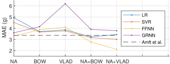
Figure 2: Mean absolute error per feature set and estimator model when training on all food types together.

VI Conclusions

In this work we have presented an approach for estimating bite weight from audio signal captured by commercially available ear buds. Using commercially available hardware is essential to enable higher adoption rates for such dietary monitoring approaches, since they reduce invasiveness and discomfort of the end user.

Our approach uses a combination of non-audio and audio features which are used to train estimation models. We evaluate on an in-house dataset of approximately $2$ hours. Our best results are obtained by training food-specific GRNN models and non-food-specific FFNN models. GRNN models yield MAE of approximately $1$ g or less, and FFNN yield a total MAE of $2.12$ g. We also compare with an existing algorithm from literature and achieve lower errors for all cases.

An important limitation of our approach is that it requires annotations for the start and stop time-stamps of individual chews, as well as food type annotations (for food-type–specific models). Future work includes evaluating on bigger and more diverse datasets with more food types and different data-capturing conditions (closer to free-living) as well as evaluating in combination with audio based chewing detectors and automatically detected food types.

References

- [1] O. Amft, H. Junker, and G. Troster, “Detection of eating and drinking arm gestures using inertial body-worn sensors,” in ISWC’05, 2005, pp. 160–163.
- [2] E. Sazonov and J. M. Fontana, “A sensor system for automatic detection of food intake through non-invasive monitoring of chewing,” IEEE Sensors Journal, vol. 12, no. 5, pp. 1340–1348, 2012.
- [3] H. Kalantarian, N. Alshurafa, and M. Sarrafzadeh, “A wearable nutrition monitoring system,” in 2014 11th BSN, 2014, pp. 75–80.
- [4] M. Farooq and E. Sazonov, “Segmentation and characterization of chewing bouts by monitoring temporalis muscle using smart glasses with piezoelectric sensor,” IEEE JBHI, vol. 21, no. 6, pp. 1495–1503, 2017.
- [5] O. Amft and G. Troster, “On-body sensing solutions for automatic dietary monitoring,” IEEE Pervasive Computing, vol. 8, no. 2, pp. 62–70, 2009.
- [6] C. Sonoda et al., “Associations among obesity, eating speed, and oral health,” Obesity Facts, vol. 11, no. 2, pp. 165–175, 2018.
- [7] V. Papapanagiotou et al., “A novel chewing detection system based on PPG, audio and accelerometry,” IEEE JBHI, vol. 21, no. 3, pp. 607–618, 5 2017.
- [8] R. S. Mattfeld, E. R. Muth, and A. Hoover, “Measuring the consumption of individual solid and liquid bites using a table-embedded scale during unrestricted eating,” IEEE JBHI, vol. 21, no. 6, pp. 1711–1718, 2017.
- [9] K. Kyritsis, C. Diou, and A. Delopoulos, “Modeling wrist micromovements to measure in-meal eating behavior from inertial sensor data,” IEEE JBHI, vol. 23, no. 6, pp. 2325–2334, 2019.
- [10] ——, “A data driven end-to-end approach for in-the-wild monitoring of eating behavior using smartwatches,” IEEE JBHI, vol. 25, no. 1, pp. 22–34, 2021.
- [11] K. Kyritsis et al., “Assessment of real life eating difficulties in parkinson’s disease patients by measuring plate to mouth movement elongation with inertial sensors,” Scientific Reports, vol. 11, no. 1, p. 1632, 1 2021.
- [12] S. Wang, G. Zhou, L. Hu, Z. Chen, and Y. Chen, “Care: Chewing activity recognition using noninvasive single axis accelerometer,” in UbiComp, ser. UbiComp/ISWC’15 Adjunct. New York, NY, USA: Association for Computing Machinery, 2015, p. 109–112.
- [13] S. Wang et al., “Eating detection and chews counting through sensing mastication muscle contraction,” Smart Health, vol. 9-10, pp. 179–191, 2018, cHASE 2018 Special Issue.
- [14] Y. Lu et al., “gofoodtm: An artificial intelligence system for dietary assessment,” Sensors, vol. 20, no. 15, 2020.
- [15] ——, “A multi-task learning approach for meal assessment,” in Proceedings of the Joint Workshop on Multimedia for Cooking and Eating Activities and Multimedia Assisted Dietary Management, ser. CEA/MADiMa ’18. New York, NY, USA: Association for Computing Machinery, 2018, p. 46–52.
- [16] V. Papapanagiotou, C. Diou, and A. Delopoulos, “Chewing detection from an in-ear microphone using convolutional neural networks,” in EMBC 2017, 2017, pp. 1258–1261.
- [17] O. Amft, M. Kusserow, and G. Troster, “Bite weight prediction from acoustic recognition of chewing,” IEEE TBE, vol. 56, no. 6, pp. 1663–1672, 2009.
- [18] V. Papapanagiotou, C. Diou, J. van den Boer, M. Mars, and A. Delopoulos, “Recognition of food-texture attributes using an in-ear microphone,” in ICPR 2020, Part V, LNCS 12665 proceedings. Cham: Springer International Publishing, 2020 [in press].
- [19] D. Specht, “A general regression neural network,” IEEE Transactions on Neural Networks, vol. 2, no. 6, pp. 568–576, 1991.