Exact Pareto Optimal Search for Multi-Task Learning and Multi-Criteria Decision-Making
Abstract
Given multiple non-convex objective functions and objective-specific weights, Chebyshev scalarization (CS) is a well-known approach to obtain an Exact Pareto Optimal (EPO), i.e., a solution on the Pareto front (PF) that intersects the ray defined by the inverse of the weights. First-order optimizers that use the CS formulation to find EPO solutions encounter practical problems of oscillations and stagnation that affect convergence. Moreover, when initialized with a PO solution, they do not guarantee a controlled trajectory that lies completely on the PF. These shortcomings lead to modeling limitations and computational inefficiency in multi-task learning (MTL) and multi-criteria decision-making (MCDM) methods that utilize CS for their underlying non-convex multi-objective optimization (MOO). To address these shortcomings, we design a new MOO method, EPO Search. We prove that EPO Search converges to an EPO solution and empirically illustrate its computational efficiency and robustness to initialization. When initialized on the PF, EPO Search can trace the PF and converge to the required EPO solution at a linear rate of convergence. Using EPO Search we develop new algorithms – PESA-EPO, that approximates the PF for a posteriori MCDM, and GP-EPO for preference elicitation in interactive MCDM; experiments on benchmark datasets confirm their advantages over competing alternatives. EPO Search scales linearly with the number of decision variables which enables its use for training deep networks. Empirical results on real data from personalized medicine, e-commerce and hydrometeorology demonstrate the efficacy of EPO Search for deep MTL.
1 Introduction
Multi-objective optimization (MOO) has numerous real-world applications ranging from engineering design to public sector planning (Stewart et al. 2008). A MOO problem can have multiple, possibly infinite, Pareto optimal (PO) solutions, represented by the Pareto front (PF). A MOO problem is often solved by scalarization that transforms it to a single objective optimization (SOO) problem. A widely used technique, in optimization, decision analysis and more recently, in artificial intelligence (see, e.g., Miettinen (1998), Reeves and MacLeod (1999), Ozbey and Karwan (2014), Daulton et al. (2022)), is the weighted Chebyshev (or Tchebycheff) scalarization (CS). Given objective functions , for , on a decision or (feasible) solution space and an input weight vector , CS minimizes the objective with maximum relative weighted value:
| (1) |
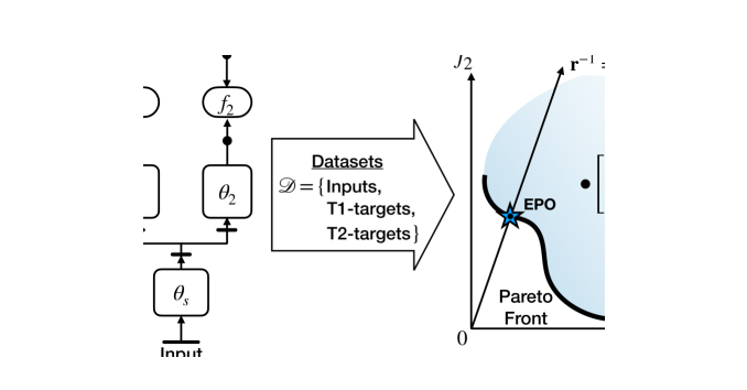
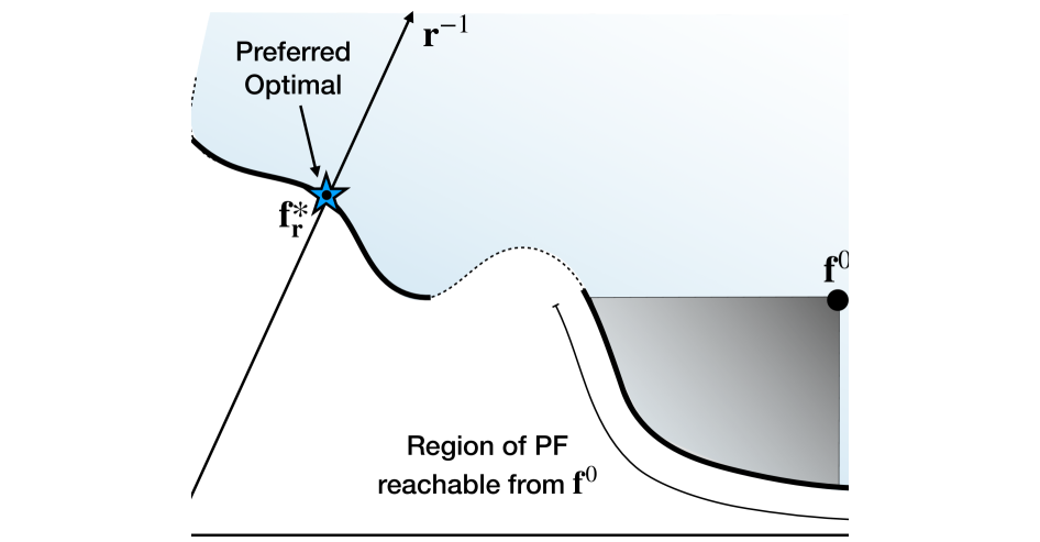
where is the element-wise product operator. A key advantage of CS, over alternative scalarizations, is that it satisfies the necessary and sufficient conditions for modeling all PO solutions of a non-convex MOO problem – the complete PF can be obtained by varying the weight values (Steuer et al. 1993, Kaliszewski 1995). The solution to (1), in general (weak PO solutions are an exception, see §2.1), lies at the intersection of the PF and the ray as shown in Figure 1(b). We call this an Exact Pareto Optimal (EPO) solution.
In this paper, our focus is on first order methods, which can scale to high-dimensional solution spaces, to find EPO solutions for differentiable ’s. To the best of our knowledge, extant literature does not provide a robust first-order iteration strategy with convergence guarantees to find EPO solutions. A first order method like gradient descent to solve (1) has the following practical and theoretical limitations. First, it uses gradients of only one of the objectives in each iteration, which changes frequently around the ray. As a result, there are oscillations in the trajectory, which slows convergence during descent. Second, if the gradient magnitude vanishes for the objective with highest weighted value, descent stagnates. In such cases, movement in each iteration is negligibly small. Third, when initialized with a PO solution, it does not guarantee that the trajectory to the required EPO solution remains on the PF. Further, the non-differentiable function in the norm of (1) makes convergence rate analysis for gradient-based methods non-trivial. These shortcomings lead to computational inefficiency and modeling limitations in methods, such as those outlined below, that utilize CS in solving their underlying non-convex MOO problems.
Consider neural multi-task learning (MTL) where each objective is a loss function (usually non-convex) for a task and a MOO solution corresponds to trained neural network parameters. Linear scalarization (that solves ) is commonly used to train MTL models, where the weights specify relative priorities among tasks. CS is theoretically advantageous for non-convex functions and is also more interpretable (see §2.1.2, 2.3). However, first order solvers that optimize the min-max formulation in (1) face challenges during training of deep networks due to the aforementioned problems of oscillations and stagnation. Since the gradient of only one of the objectives is used in each iteration, optimization effectively leads to just single-task learning which ultimately deteriorates the model’s predictive accuracy. The same problem occurs when a relatively high priority is given to a task – the other tasks are completely ignored during training. This may be alleviated through second order methods but they are not scalable to high-dimensional parameter spaces in deep networks.
As another example, consider multi-criteria decision-making (MCDM), where the decision maker (DM) has to choose the most suitable PO solution of the underlying (non-convex) MOO problem. We study two approaches – (i) a posteriori methods, where multiple PO solutions are computed that collectively provide an approximate view of the PF and enables the DM to select one desired solution and (ii) interactive methods, where the DM progressively articulates preferences among solutions and proceeds towards a satisfactory solution while interacting with the MOO solver. The DM’s preferences are assumed to follow an (unknown) utility function that can score and order PO solutions, and is monotonic, i.e., a solution that Pareto dominates another has higher utility. In both these cases, there are multiple calls to the MOO solver, each time after a PO solution is obtained. If the min-max formulation (1) is used, and the trajectory between consecutive solutions is not on the PF, the MCDM approach has high computational burden. Moreover, such solvers also need to be re-initialized and re-started at PF discontinuities where they may halt prematurely.
We design a new approach, called EPO Search, to efficiently find EPO solutions for non-convex MOO, which addresses these limitations. Using EPO Search we develop techniques that advance the state-of-the-art in first order methods for (a) PF approximation for a posteriori MCDM, (b) preference elicitation in interactive MCDM and (c) training deep multi-task neural networks. The four main contributions of this paper are as follows.
1. We design and analyze search direction strategies that balance the dual goals of moving towards the PF as well as towards the ray, which equip us to combine gradient descent with carefully controlled ascent in objectives with less relative weights to avoid their local minima. By using a linear combination of all objective gradients, while moving in a balancing search direction, EPO Search avoids the problems of oscillations and stagnation. We prove, under mild assumptions and without assuming convexity, that, from a random initialization, EPO Search converges to the EPO solution, or, if an exact solution does not exist, to a PO solution closest to the ray. When initialized at an arbitrary PO solution, we prove that EPO Search converges to the desired EPO solution with a trajectory close to the PF and under mild regularity conditions, we prove that the convergence rate, even for non-convex objectives, is linear. EPO Search scales linearly with the gradient dimension per iteration and thus, can efficiently find (local) EPO solutions in high-dimensional solution spaces. We extend EPO Search for solving constrained MOO problems without compromising on its computational efficiency. Our empirical results on benchmark MOO problems support the theoretical claims of scalability and accuracy of EPO Search.
2. Using PESA (Stanojević and Glover 2020) to generate a diverse set of weight vectors, we develop the algorithm PESA-EPO to approximate the PF. Leveraging the PF tracing ability of EPO Search, PESA-EPO efficiently finds multiple PO solutions without multiple optimizer calls, and without premature halts at PF discontinuities. On several benchmark convex and non-convex MOO problems, both with and without constraints, PESA-EPO leads to better or comparable PF approximation in lower execution time, compared to competing gradient-based as well as evolutionary MOO algorithms.
3. In probabilistic preference elicitation, a Gaussian Process (GP), which can model any (including non-linear and non-convex) function, is used to learn the DM’s unknown utility. Pairwise comparisons from the DM are used to interactively learn the GP parameters in a Bayesian active learning framework, where, in each interaction, the DM specifies her preference between the two presented PO solutions. To reduce their computational burden, previous approaches, e.g., Chin et al. (2018), Zintgraf et al. (2018), sample these PO solutions from a discrete subset of the solution space (see §2.2.2), which affects their accuracy of preference learning. Further, since sampling from the GP does not guarantee a PO solution, previous methods impose monotonicity constraints during or employ postprocessing heuristics after sampling from the GP; these steps either deteriorate performance or increase computational time. We address these limitations by developing GP-EPO where we explore the PF at high resolution, by sampling rays (in a lower -dimensional space, instead of the entire solution space) and then efficiently find PO solutions through EPO Search to present to the DM. Our approach obviates the need to explicitly model monotonicity constraints. Further, over the interactions, GP-EPO moves from one EPO solution to another with linear convergence rate. Evaluation on benchmark problems show that GP-EPO learns the utility with substantially better accuracy, compared to extant GP-based methods, in just a few interactions.
4. In MOO-based neural MTL, which models tradeoffs among objectives, previous methods either do not use task-specific priorities or yield multiple PO solutions for an input set of diverse relative priorities. An EPO solution models task priorities specified by the ray, thus prioritizing tasks that are challenging to learn; without losing the benefits of MTL that allows shared learning from other datasets and tasks. Compared to gradient descent to solve (1) for network training, EPO Search offers a more robust iterative procedure that overcomes the problems of oscillation and stagnation; further, its ability to use the gradients of all objectives and escape minima of lower priority objectives leads to improved MTL. The per-iteration complexity of EPO Search remains linear in the gradient dimensions (similar to the best previous methods that neither use input priorities nor allow regularization constraints) enabling its use for deep MTL networks. We evaluate the efficacy of EPO Search for MTL on three real datasets from different domains: personalized medicine, e-commerce and hydrometeorology. In all cases, the use of EPO Search leads to higher predictive accuracy compared to single-task learning, the direct use of linear and Chebyshev scalarization during training and competing MTL models.
The rest of the paper is organized as follows. Background and related work are presented in §2. We then describe our theory and algorithms for EPO Search in §3. Algorithms PESA-EPO, GP-EPO and EPO Search for MTL are described in §4. Experimental results are in §5, followed by our concluding discussion in §6.
2 Background and Related Work
We describe relevant concepts and related work from three streams of literature – multi-objective optimization (MOO), multi-criteria decision making (MCDM) and multi-task learning (MTL).
2.1 Multi-Objective Optimization
We consider a multi-objective optimization (MOO) problem with non-negative differentiable objective functions, for , where . This formulation is fairly general, since problems with different specifications can be converted to this form. For instance, if an objective is negative at its minimizer, i.e., , then, to make it non-negative, one can reformulate as , where is a lower bound on the minimum: . The vector consisting of the lower bounds of all objectives is called as a “utopia” point, which makes a non-negative vector valued function. We develop MOO algorithms for unconstrained problems in the main paper, and extend them to solve constrained MOO problems in .
We use to denote both a vector valued function and a point in the Objective Space , which should be unambiguous from the context. The range of , denoted by , is a subset of the positive cone . The partial ordering for any two points , denoted by is defined by , which implies for every and strict inequality occurs when there is at least one for which . Geometrically, means that lies in the positive cone pivoted at , i.e., , and .
For a minimization problem, a solution is (weakly) dominated by another solution if () . Note that if is not dominated by , i.e. . A solution is Pareto optimal (PO) if it is not dominated by any other solution. Weak PO solutions are weakly dominated by other PO solutions. The set of all global PO solutions is , and the set of local PO solutions is:
| (2) |
where is an open neighbourhood of in . Note that . The set of multi-objective values of the PO solutions, , is called the Pareto front (PF). Excellent surveys on MOO can be found in, e.g., Gandibleux (2002), Wiecek et al. (2016).
2.1.1 Descent Methods for Converging to the Pareto Front.
Gradient-based MOO solvers, such as in Fliege and Svaiter (2000), Vieira et al. (2012), find a PO solution by starting from an arbitrary initialization and iteratively obtaining the next solution that dominates the previous one (i.e., , where ), by moving against a direction with a step size as , such that there is descent in every objective, . This can happen only if has positive angles with the gradients of every objective function at :
| (3) |
we call such a a descent direction. Note, by convention, the move is against , i.e., along .
Désidéri (2012) showed that descent directions can be found in the Convex Hull of the gradients,
| (4) |
where is the dimensional simplex. Their multiple gradient descent algorithm (MGDA) converges to a local PO by iteratively using the descent direction: Although descent-based methods provide convergence guarantees (Tanabe et al. 2022), they cannot find EPO solutions.
2.1.2 Scalarization.
The popular approach of linear scalarization (LS) of a MOO problem with an input weight vector finds
| (5) |
If the range of , i.e. , is convex then for every , there exists an such that . The weight vector is an element in the dual of the objective space (Luenberger 1997), and represents a hyperplane in the objective space. The hyperplane of at has to be both a tangent and a support to the PF, i.e., for all . If any of the objectives is non-convex, i.e., the range is a non-convex set, LS cannot guarantee to reach every optimal point in the PF by varying the weights (Boyd and Vandenberghe (2004)[Ch 4.7]), because the tangent hyperplane at a point on the PF is not necessarily a support if is non-convex. Moreover, even a single vector can have non-unique PO solutions; see Figure 1(a).

Definition 1.
Given a weight vector , an Exact Pareto Optimal (EPO) solution belongs to the set:
| (6) |
For any EPO solution , is a point on the PF intersecting the ray towards (see Figure 1(b)), i.e., is perfectly proportional to the ray. CS, i.e., a solution to (1), is an EPO solution, as illustrated in Figure 1(b), because, its level set can also be written as , the negative orthant pivoted at . Therefore, if is a singleton set then the corresponding solution is an EPO point w.r.t. .
Although for convex MOO problems LS and CS may be considered equivalent (Luque et al. 2007), they differ for non-convex MOO. Unlike LS, CS provides both necessary and sufficient condition for weak Pareto optimality of non-convex MOO problems. CS has extensions such as augmented CS (Steuer 1989, Miettinen 1998) that eliminates the corner case of weak PO solutions. However, such extensions lose the exactness property of CS for its strong PO solutions, and we leverage the exactness property for our algorithms. These scalarization methods, their variants and generalizations (Gembicki and Haimes 1975, Pascoletti and Serafini 1984, Wierzbicki 1986, Marler and Arora 2004) specify a desired PO solution through their parameters. However, to our knowledge, there is no robust first-order iterative strategy that guarantees convergence to a desired EPO solution starting from a random initialization.
2.2 Multi-Criteria Decision-Making (MCDM)
MCDM aims to solve decision-making problems involving multiple conflicting objectives (Wallenius et al. 2008, Köksalan and Wallenius 2012). We focus on continuous MCDM problems, with differentiable objectives, where the solution alternatives are (or can relaxed to be) in a continuous space. Based on how a DM participates in the solution process MCDM approaches can be categorized into (Hwang et al. 1979, Miettinen 1998): (i) a priori methods where preferences are specified before the MOO problem is solved (ii) a posteriori methods where multiple PO solutions are computed from which the DM selects one and (iii) interactive methods where the DM progressively articulates preferences and, along with the MOO solver, iteratively proceeds towards a satisfactory solution.
In each of these categories, there are various ways to articulate preferences (Miettinen 1998). Preferences may be articulated by comparison of PO solutions, e.g., through pairwise comparisons (e.g., Korhonen et al. (1984), Köksalan and Sagala (1995)) or selection from a set of solutions (e.g., Greco et al. (2010)). A utility function that assigns a scalar value to every objective vector (Keeney et al. 1993), may be used to model the DM’s preferences and create a total ordering among the PO solutions. The utility is commonly assumed (Fishburn 1968) to satisfy the monotonicity property: for any two alternatives and , if dominates (i.e. ), then , where . The oracle solution maximizes the DM’s (unknown) utility:
| (7) |
The DM’s utility may be learnt in both a posteriori and interactive MCDM, e.g., in Jing et al. (2019), a utility function is constructed using the PF approximation from an a posteriori method; preference elicitation (PE) methods may be used in interactive MCDM (see §2.2.2).
2.2.1 A Posteriori Methods and Pareto Front Approximation.
In a posteriori methods, the ability of an algorithm to quickly and evenly approximate the PF is crucial Das and Dennis (1997, 1998). Many Multi-Objective Evolutionary Algorithms (MOEA) have been developed to approximate the PF, e.g., (Zhang and Li 2007, Li and Zhang 2009, Qi et al. 2014, Zhang et al. 2015, Deb et al. 2002, Deb and Jain 2014, Zhang et al. 2018, Li et al. 2019). They are effective in practice and scale well to many objectives (Emmerich and Deutz 2018). However, they do not scale well to high-dimensional solution spaces.
In gradient-based MOO, a scalarization method is run several times with a diverse set of parameters to generate well spread out PF approximations. The simple LS method fails to generate evenly spread solutions from a set of evenly spread weights (Das and Dennis 1997). To address this problem, Das and Dennis (1998) developed a direction-based scalarization method called Normalized Boundary Intersection (NBI) that finds PO solutions along many directions normal to the Convex Hull of the Individual Minima (CHIM) of the objective functions. Several improvements of NBI have been proposed (Ismail-Yahaya and Messac 2002, Shukla 2007, Siddiqui et al. 2012) but they remain computationally inefficient as they require re-initializations at PF discontinuities and do not scale well to many objectives. Stanojević and Glover (2020) proposed a recursive sampling strategy Pattern Efficient Set Algorithm (PESA) that samples weights/directions from the simplex spread uniformly, and scales well with number of objectives. They used an NBI type scalarization called Targeted Direction Model (TDM) to find direction specific solutions. However, similar to NBI, their method also has to solve many SOO problems, one for each direction ray.
2.2.2 Preference Elicitation for Interactive MCDM.
Preference Elicitation (PE) aims to infer the DM’s unknown utility function using the DM’s responses to queries in interactive MCDM. We assume the queries to the DM are in the form of pairwise comparison of alternatives, which is cognitively less demanding compared to other query types (such as value assignment) (Tesauro 1988, Forgas 1995). Methods such as Conjoint Analysis (Rao 2010, Angur et al. 1996) and Best-Worst Method (Oztas and Erdem 2021) are well-known for discrete MCDM problems. In continuous MCDM, the utility is a fixed parametric function of the objective values, e.g., Chebyshev utility that uses CS (Steuer 1989, Steuer et al. 1993, Dell and Karwan 1990, Ozbey and Karwan 2014, Reeves and MacLeod 1999); and in Preference Robust Optimization (PRO), where Vayanos et al. (2020) model the utility as a linear function and Haskell et al. (2018) model it as a quasi-concave function. These methods cannot model non-convex PE problems, where either the MOO problem or the utility function could be non-convex. See Appendix G for an extended discussion.
In contrast to these methods, the Bayesian active learning framework for PE (Eric et al. 2007, Zintgraf et al. 2018, Roijers et al. 2021) uses Gaussian Process (GP) to model the utility that can model any class of functions. Further, this can model uncertainty in the DM’s stated preferences and works well with less data – requiring just a few interactions with the DM to learn preferences (Deisenroth et al. 2013). Appendix H has an overview of Bayesian optimization with GP.
The prior for the unknown utility function, , is modelled as , where and are the mean and covariance functions respectively. Learning proceeds by alternating between querying the DM based on the current GP and updating the GP posterior after obtaining the resulting comparison from the query. Thus, the observational data from which the GP is learnt is , where is the number of pairwise queries to the DM, and an ordered pair represents the DM’s comparison of two alternatives as “ is preferred to ”, suggesting . If the DM values both alternatives equally, then the dataset can include both and , making . Inconsistencies in DM’s response are modelled as additive noise: , where . For such noisy pairwise comparison data, Chu and Ghahramani (2005) developed a probit likelihood model for , wherein the posterior, , is analytically non-tractable, but can be approximated to a GP using Laplace approximation. In the beginning, when there is no comparison data, , the GP prior is usually initialized with a zero mean function.
Let be the discrete set of alternatives presented to the DM, and be the incumbent solution, where is preferred to all other solutions in . In each iteration, selection of a new alternative to create the next query is done using an acquisition function . A commonly used acquisition function in previous works on interactive PE, e.g., Eric et al. (2007), is the Expected Improvement (Močkus (1975)) function which is optimized to suggest a new alternative:
| (8) |
where is a discrete subset of . The DM is then asked to compare between and . The new comparison datapoint is included in the dataset, and the posterior is updated to to approximate . This iterative procedure is continued until, either for a small or the DM is satisfied with .
Previous GP-based approaches have two important limitations. First, they optimize over a discrete subset, , of the entire search space, because and can be highly non-linear, which renders the global optimization of (8) computationally expensive, especially if is high dimensional. Decreasing the size of the discrete subset improves computational efficiency but reduces accuracy of preference learning. Second, additional monotonicity constraints need to be enforced because sampling from a GP does not guarantee a PO solution. Several heuristics to address this problem have been proposed (Chin et al. 2018, Zintgraf et al. 2018, Roijers et al. 2021) that either deteriorate performance or increase the computational burden.
2.3 Multi-Task Learning
Multi-Task Learning (MTL) has been studied extensively in machine learning (see, e.g., Zhang and Yang (2021)). Learning multiple tasks together leads to inductive bias towards hypotheses that can explain more than one task and has been found to improve model generalization in machine learning (Caruana 1997).
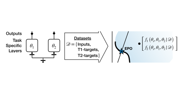
A multi-task neural network is trained for multiple tasks simultaneously and inductive transfer is enabled through shared parameters, most commonly through fixed layers common to all tasks (Ruder 2017) (Appendix I has an overview of neural networks). Figure 2 (left) shows a schematic of a MTL network for two tasks T1, T2 with objective (loss) functions respectively. The network has one or more shared layers with parameters and task-specific layers with parameters that are learnt during training. For conflicting tasks, we cannot assume that parameters learned through SOO are effective across all tasks as trade-offs among the tasks are not explicitly modeled. In such cases, PO solutions from MOO yield better models, as shown by Sener and Koltun (2018). They extended MGDA to handle high-dimensional gradients, thereby making it usable for deep MTL models. However, their method finds a single arbitrary PO solution and cannot be used by MTL designers to explore solutions with different trade-offs. This is illustrated in Figure 1(b).
Current MTL approaches which use MOO for training, do not explicitly model task-specific priorities. While LS has been used in SOO settings, to our knowledge, CS, has not been used in MTL. Task-specific priorities through CS can be effected through EPO Search for model training. The related, Pareto MTL (PMTL) algorithm by Lin et al. (2019), finds multiple solutions on the PF through a decomposition strategy and may be modified to find EPO solutions. They use several reference vectors , each of unit magnitude, to partition the solution space into sub-regions . With this decomposition, if , then the EPO solution . There are two phases in their algorithm. In phase one, starting from a random initialization, they find a point , such that the corresponding . In phase two, they iterate using descent-only directions to reach a PO . However, their method does not guarantee that the outcome of second phase also lies in . Moreover, to reach a desired EPO solution, they have to increase the number of reference vectors exponentially with increase in number of objectives . Their method, by design, does not reach an EPO solution but only in the sub-regions of the PF between the references (see §5.1 and Appendix D.3).
3 Exact Pareto Optimal Search Algorithms
Our key idea is to gain control over the trajectory of objective vectors in the objective space so that an iterative algorithm can efficiently reach the desired solution. To anchor the iterations, we design suitable vector fields on by defining their direction:
Definition 2 (Anchoring Direction).
We call an element of the tangent space of the objective space an Anchoring direction, denoted by , where is the footpoint.
To find the EPO solution by an iterative procedure, it is not sufficient to advance only along the descent directions (3) because it leads to an arbitrary solution in the PF. Moreover, even if for every , the solution may not lie on the ray (figure 1(b)), and hence will not satisfy the condition in (6). Therefore, apart from a descent direction that moves the objective vector closer to the PF, we also need to consider a search direction (tangent space of ) that moves the objective vector “closer” to the ray. To find such a direction, in §3.1, first we define a general Proportionality Gauge (PG) to measure the closeness between and and analyze its properties. Then we present three specific examples of PGs whose (scaled) gradient fields, called as balancing anchor directions, can advance the iterates closer towards the ray, while maintaining . In §3.2, we present descending anchor direction to advance closer to the PF with . We then develop two MOO algorithms in §3.4 and §3.5 to reach an EPO solution, starting from a random initialization in and respectively, by using both balancing and descending anchor directions.
3.1 Proportionality of Vectors and Balancing Direction
Definition 3 (Proportionality Gauge).
A function is called a Proportionality Gauge, if, for any given inputs and , we have:
-
1.
only when is a positive scalar multiple of , and
-
2.
is differentiable w.r.t and increases monotonically along , for , with increment in .
For a given weight vector and a point , we define an anchor direction as for some . We use it to characterize a search direction to move the objective vector closer to ray.
lemmaancr If all the objective functions are differentiable, then for any direction satisfying , where is the Jacobian of at , and , there exists a step size such that for all
| (9a) | ||||
| (9b) | ||||
A move against the search direction of Lemma 3 reduces the variations in relative objective values to make them equal: brings balance among the values of . Therefore, we call this a Balancing Search Direction, and a Balancing Anchor Direction. We call a balancing anchor direction Scale Invariant to if for all . Using the scale invariant property, we further narrow down the characteristics of a balancing search direction.
theoremfdeqa If a balancing anchor direction is scale invariant to and all the objective functions are differentiable at , then moving against a direction with , for some , yields a non-dominated solution such that is closer to the ray than .
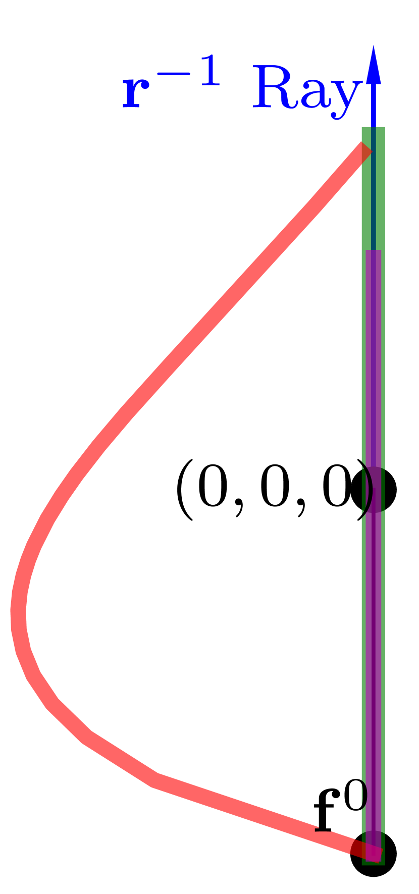
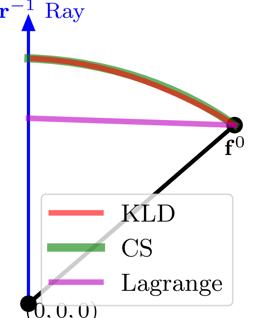
Note that for a small step size , the difference between the consecutive objective vectors can be approximated as from the first order Taylor series expansion. So, the search direction in Theorem 3 moves the objective vector against the balancing anchor direction (i.e., along ) in the objective space. In the following, we propose three different functions – using Cauchy–Schwarz inequality, Lagrange’s identity and KL divergence – for gauging the proportionality between two vectors and analyze them based on their respective balancing anchor directions.

3.1.1 Proportionality Gauge from Cauchy–Schwarz (CSZ) Inequality:
The CSZ inequality of our non-zero vectors , , is tight (equal) when both the vectors are proportional to each other. Rearranging the terms to one side, we get the following
| (10) |
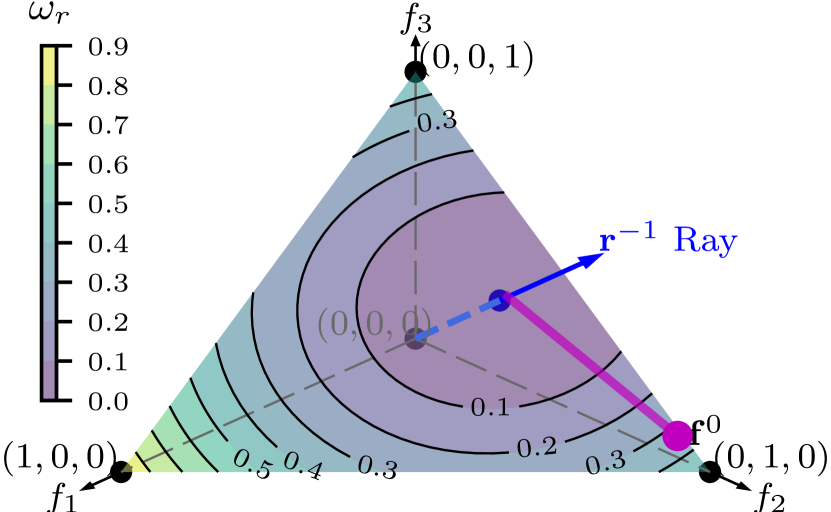
which satisfies properties 1 and 2 of a proportionality gauge. Figure 3(a) shows the corresponding in case of objectives and a particular weight vector. We formulate its anchoring direction as
| (11) |
where is the normalization of a vector . This is scale invariant to and has the same direction as the gradient . Its main benefit is drawn from the following. {restatable}claimcsaf The anchor direction in (11) is always orthogonal to the objective vector : . The change in consecutive objective vectors is approximately aligned to . Therefore, Claim 3.1.1 suggests that . In other words, since is an all positive vector, changes in some objectives are positive and others are negative. The advantage of an orthogonal anchoring direction lies in its ability to simultaneously ascend and descend which helps in escaping a PO solution that is not an EPO solution (formalized in Theorem 3.5.1).
Since is a linear combination of and , the trajectory of the objective vectors lies in the span of . However, it does not result in the shortest trajectory to reach ray (see Figure 3(e)). The shortest path between a point and the ray is the line segment from orthogonal to the ray, wherein every , and hence , should be orthogonal to the ray at all .
3.1.2 Proportionality Gauge from Lagrange’s Identity:
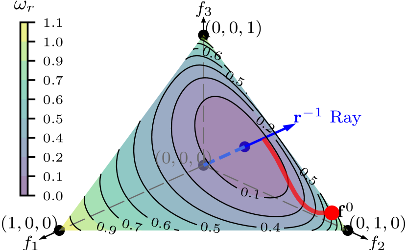
The difference between both sides of CSZ inequality, known as Lagrange’s Identity, can be a proportionality gauge:
| (12) |
It satisfies both conditions 1 and 2 of a proportionality measuring function. The factor in (12) makes its anchoring direction scale invariant to and we equate to the gradient :
| (13) |
This anchor direction can yield the trajectory of shortest path, as shown in figure 3(e). {restatable}claimlgnaf The anchor direction in (13) is always orthogonal to the ray: . Note, when and are not proportional, and are not orthogonal as . As a result, this anchor direction may not escape a PO solution that is not EPO, because orthogonality of and is a necessary condition for non-convergence at a non-EPO solution in Theorem 3.5.1. In its proof, we discuss a corner case where the in (13) cannot escape a non-EPO solution.
3.1.3 Proportionality Gauge from KL Divergence:
In §A.1, we present this proportionality gauge, which measures the KL divergence between and the uniform vector . Figure 3(c) shows the corresponding in case of 3 objectives. However, we do not use it since its anchoring direction neither produces the shortest path nor belongs to , as shown in Figures 3(c) and 3(d).
We compare the proportionality gauges and their anchor directions in §A.2.
3.2 Descending Direction
When the iterate is on or close to the ray, i.e. for small , to reach the EPO solution, we require descent for every objective. To guarantee descent for all, we choose
| (14) |
Because if the search direction satisfies , then for all as , hence would be a descent direction. When , we call it a Descending Anchor direction. It can be considered as the gradient field of .
3.3 Quadratic Program for Modelling the Search Direction
We now develop iterative methods to find the EPO solution w.r.t a weight vector . In each iteration, we solve a Quadratic Programming (QP) problem to obtain a search direction , the tangent plane (or cone, if is constrained, see §B) at , such that it corresponds to an anchor direction , the tangent plane at .
We model the search direction as a linear combination of the objective gradients, i.e., and compute the optimal coefficients by solving
| (15) |
so that is aligned to the anchor direction as much as possible. Note that, unlike Désidéri (2012), we do not restrict to the convex hull of the positive gradients (4) to model only descent directions. With coefficients in the ball, we facilitate gradient ascent for some of the objectives whenever necessary by allowing to be in the convex hull of both positive and negative gradients:
| (16) |
3.4 EPO Search from Random Initialization
When the goal is to find the EPO solution for a given starting from a random initialization , we use the balance mode with the anchor direction from Lagrange’s identity (13) for every iteration until is (nearly) proportional to , for a small . After that, we use the descent mode until convergence, for a small . We extend the QP in (15) (see §B.1 for its extension to constrained MOO problem) to solve
| (17a) | ||||
| s.t. | (17b) | |||
| where | (17c) | |||
is the index set of maximum relative objective values. We call the resulting a Non-Dominating Search Direction, because it can yield a solution that is not dominated by , i.e. . We state this formally for the balance mode in Lemma 17 and descent mode in Lemma 17 with a regularity assumption. In the terminology of differentiable maps, is a Regular Point of the vector valued function , if its Jacobian is full rank. {restatable}lemmadndbal If is a regular point of the differentiable vector function in a balance mode, i.e. , then the non-dominating direction obtained from QP (17) makes
-
1.
non-negative angles with the gradients of maximum relative objectives: (17c),
-
2.
a positive angle with the balancing anchor direction (13) in the objective space: .
lemmadnddes If is a regular point of the differentiable vector function in a descent mode, i.e. , then the non-dominating direction obtained from QP (17) makes a non-negative angle with every gradient, , and a positive angle with at least one gradient.
A positive angle with the gradient means moving against will reduce the corresponding objective value. Lemmas 17 and 17 are true even without the constraint (17b) ((42d) for constrained MOO) if , where is defined in (16). Also, the Lemmas are true at certain irregular points whose Jacobian matrices are not full rank (discussed in the proof).
We summarize our EPO Search procedure for random initialization in Algorithm 1 . A practically useful variation to improve the descent mode is discussed in Appendix D.2.
3.4.1 Convergence.
We prove the convergence of Algorithm 1 in two steps. First we define an admissible set that contains potential objective vectors to which the EPO Search in Algorithm 1 can reach. Then we prove that the sequence of sets converges to , the set containing the EPO solutions. The results hold true for both constrained and unconstrained MOO problems, as detailed in the proofs.
To characterize the properties of obtained by moving against , we define some sets in that are illustrated in Figure 4. The set of all attainable objective vectors that dominate the is denoted as (18). The set of all attainable objective vectors that have better proportionality than is denoted as (19). During a descent mode , and in a balance mode . For the iteration, we define a point as in (20), where is the maximum relative objective value. Finally, using , we define the admissible set111The admissible set of an iteration in the CS (1) is , where . of an iteration in EPO Search Algorithm 1 as (3.4.1) for any mode, balance or descent.
| (18) | ||||
| (19) | ||||
| (20) | ||||
| (21) | ||||
Clearly, the admissible set contains all the points in that dominate the , . Moreover, when , it also has points with better proportionality than , . Therefore, using Lemmas 17 and 17, we can state the following. {restatable}lemmaadms If is a regular point of , there exists a step size , such that for every , the objective vector of lies in the admissible set: . We extend the regularity assumption of to all points in to state the convergence result. {restatable}theoremmntnct If is a differentiable regular vector valued objective, then the sequence of admissible sets , which correspond to the solutions produced according to Lemma 4 starting from a non-Pareto Optimal point , converges by decreasing monotonically . When is a singleton set then converges to . Note, if an EPO solution does not exist for the given preference , i.e. ray does not intersect the PF , then EPO search finds the intersection point between ray and , the boundary of the attainable objective vectors. If the ray does not intersect , then EPO search finds the point in that is maximally proportional to the ray.
3.5 EPO Search for Tracing the Pareto Front from
If the initialization itself is a PO solution, then we can modify the EPO search of Algorithm 1 to trace the PF from to , an EPO solution w.r.t. weight vector , and obtain new PO solutions along the trajectory. In the modified algorithm we use CSZ inequality-based anchor direction (11) in the balance mode because it is orthogonal to the objective vector (see Claim 3.1.1), and guarantees to escape the local PO at to a new point (justified in the proof of Theorem 3.5.1). However, if we use only the balance mode until for a small , the trajectory may drift away from the PF, especially for convex objective functions (see §D.1.1). Therefore, to ensure that the objective vectors in EPO search trajectory stay close to the PF, we alternate between the balance mode and descent mode in every iteration. To ensure the proportionality gauge (10) does not increase in the descent mode, we extend the QP (15) (see §B.2 for its extension to constrained MOO)
| as follows | ||||
| (22a) | ||||
| s.t. | (22b) | |||
| and | (22c) | |||
where is the balancing anchor direction (11), and is an indicator variable for descent mode, which applies the constraint (22b) only in the descent mode. But the stopping criteria is checked only in the balance mode: the goal is to keep balancing the relative objective vector until it is proportional to uniformity . Note, this balance mode ignores the constraints in (17b) for objectives of (17c) because, if is on (close to) the PF, then an for may need to increment to move towards the EPO solution. Algorithm 2 summarizes the entire method.
3.5.1 Convergence.
We prove the contra-positive: convergence is not achieved until the iterate is close to , and keeps decreasing. At an , the set of descent directions is given by A necessary condition to check if is a PO solution, i.e., , is given by Pareto Criticality:
| (23) |
The Jacobian at an is not full rank. However, is called a Regular Pareto Optimal solution if its Jacobian has rank (Zhang et al. 2008). Previous gradient-based methods (Fliege and Svaiter 2000, Désidéri 2012) use the Pareto criticality condition as a stopping criterion, since they use descent directions in every iteration. Therefore, they stop at any local PO solution. In contrast, our method is not designed to find for a descent direction, hence does not stop prematurely at any local PO solution; it traces the Pareto front until an EPO solution is found.
3.6 Convergence Rate and Iteration Complexity
The convergence rate of a gradient-based SOO method to reach a stationary point is well known to be sub-linear for non-convex problems and linear for convex problems (Nesterov 2004). Tanabe et al. (2022) extended this result for descent-based MOO methods to reach a Pareto stationary point: sub-linear for non-convex and linear for convex MOO problems.
EPO Search has two modes of operation. In Algorithm 1, when the random initialization is not a PO solution, first the balance mode iterations decrease the value of down towards a small value to align the objective vector to the ray. Then, the descent mode iterations decrease each objective to reach an EPO solution that also satisfies the Pareto critical condition (23). The descent mode is similar to solving a non-convex SOO problem of the objective , with sub-linear convergence rate. Here, we show that the balance mode has linear convergence rate. This result is significant because it shows that the EPO Search Algorithm 2, where the initialization is a PO solution, can converge at linear rate to the desired PO solution, even for a non-convex MOO problem. Note, Algorithm 2 traces the PF by alternating between balance and descent modes, where the descent mode does not increase but balance mode decreases .
We analyze the composite objective function to prove linear convergence of the balance mode when optimizing non-convex objectives . The following Polyak-Łojasiewicz (PŁ) type inequality (Polyak 1963, Hardt 1975, Karimi et al. 2016) is instrumental in our analysis. {restatable}lemmaplineq There exists a such that the proportionality gauges (10),(12) and their respective anchor directions in (11), (13) satisfy
| (24) |
where is the initialization, is the normalization of vector , and is as in (19). The inequality (24) suggests that the magnitude of anchor direction grows quadratically w.r.t. the value of the proportionality gauge. Our additional assumptions are as follows.
Assumption 1 (Compactness).
Assumption 2 (Smoothness).
The gradients of each objective function is Lipschitz smooth: where for all ; and . The gradient of is also assumed to be Lipschitz smooth: .
Since the Jacobian is is a smooth function, the singular values of , for , where , are also smooth functions. Note, for all due to the Pareto criticality condition (23). So far, we assumed Jacobian is full rank if and rank if , as the regularity condition. We make this assumption more specific by considering a -neighbourhood around the PF as
| (25) |
can be considered as the operating region for the balance mode of EPO Search Algorithm 1, and as the operating region of EPO Search Algorithm 2 that traces the PF.
Assumption 3 (Regularity).
There exists a such that the smallest singular value for all and the second smallest singular value for all .
With the above three assumptions, we state the linear convergence rate result. {restatable}[Convergence Rate, Iteration Complexity]theoremcvnrt If the stepsize is any , where , , , , , when (10), and and when (12), then the balance mode iterations, using either (11) or (13) as anchor direction, decrease linearly:
| (26) |
where the polynomial is positive for all . Consequently, the maximum number of iterations (iteration complexity) required to decrease down to is .
3.6.1 Time Complexity per Iteration:
Both the dimensional QP problems (17) and (22) are convex, having linear constraints and are independent of the dimension of the solution space. The former has at most inequality constraints, and the latter has at most inequality constraints; both have inequality constraints for ball. The QPs can be solved efficiently, e.g., using interior point methods (Cai et al. 2013, Zhang et al. 2021) in time. The complexity of the Jacobian matrix multiplication is . Thus, the per-iteration time complexity of both Algorithms 1 and 2 is .
4 EPO Search for MCDM and MTL
4.1 Pareto Front Approximation for A posteriori MCDM
With the tracing capability of our algorithm we can move from one PO solution to another, and discover new ones in the path. We use this feature to generate a diverse set of optimal solutions by tracing towards the EPO solutions for different weight vectors. We adopt the Pattern Efficient Set Algorithm (PESA) by Stanojević and Glover (2020) for generating a diverse set of weight vectors in the dimensional Simplex . PESA is a recursive sampling procedure to approximate the simplex . Instead of sampling , we directly sample the rays since it is directly (not inversely) associated with the anchor directions. The sampling process in PESA is as follows: given a set of rays , the next new ray is sampled as a convex combination of rays in , i.e. . This new ray creates more sets, for all , and one can recursively sample rays from these sets. Thus, the convex hull of the original set is “filled”. If consists of the axes of positive orthant in , then this recursive sampling process approximates the entire simplex.
We integrate this sampling rule with EPO Search algorithm and develop the PESA-EPO Search Algorithm 3 for approximating the PF. Instead of a set of rays, we maintain a set of PO solutions , and sample the next ray as
| (27) |
We then run EPO search (Algorithm 2) to trace the PF from to ray for each . This generates trajectories on the PF. Let be the end point of the trajectory starting at . This creates creates new sets, for all , and the same procedure is repeated recursively. The procedure starts with an initial set consisting of the optimal solutions of individual objectives, and the recursion stops at a given input depth. In the collection of points obtained from the trajectories, there could be solutions that are dominated by others. In a post-processing step, the dominated solutions are removed.
Note that, the PF may be disconnected. But the trajectories of EPO Search can move between different portions of if is one connected component, which for unconstrained MOO is trivially true, and for constrained MOO is true when the domain is a connected component. In case of a bi-objective optimization with a connected PF, a recursion depth of just can approximate the PF. Because for , the PF will be at most a -dimensional manifold, and the trajectories of traced EPO Search are also -dimensional. This is further clarified in our empirical results (§5.3).
4.2 Preference Elicitation in Interactive MCDM
The key idea of our approach is to operate in the domain of the dimensional simplex instead of the high-dimensional solution space (or its discrete subset that is used in (8) by previous methods). In our PE, the data on which the GP is learnt consists of instead of . Using a mapping defined below and EPO Search, we find PO solutions and return to .
Let , where is the extended real line, be a mapping from the simplex to the objective space defined as
| (28) |
maps (scales with factor ) a point in the simplex to a point on , the boundary of the image , if the ray intersects . If it does not intersect , then it is mapped to a vector at , since the scaling factor will be . Clearly, the image of under covers all the PO solutions, . Using EPO search Algorithm 2, for a given , we can reach and the corresponding EPO solution if it exists. Non-existence can be detected through the value of proportionality gauge, i.e. , where is the output of Algorithm 2.
Instead of modeling the GP prior for the entire , we model , where with , where and . We interactively estimate the utility for PE by maintaining a parallel dataset , where the ordered pair corresponds to the DM’s comparison of two PO solutions (see §2.2.2) by using the inverse mapping of : , and similarly for . Thus, we convert the PE for into a PE for . Analogous to in §2.2.2, we define to be the discrete set of s whose corresponding s have been presented to the DM. Similarly, the incumbent corresponds to . After updating the GP to approximate the posterior , we obtain
| (29) |
as the next suggestion, where is the acquisition function formulated using the updated and . Then we run EPO Search Algorithm 2 starting from to find , the EPO solution for . If is detected, i.e. the ray does not intersect and maps to a point at infinity, we augment the dataset with , declaring that is inferior to . Thus, we avoid optimization on the high dimensional domain of solutions , and instead do it from the domain of dimensional . We summarize our method in Algorithm 4.
GP-EPO does not estimate the utility of non-PO solutions. Although is defined for all possible alternatives, its estimation for the entire range of is unnecessary due to the monotonicity property of a utility function. Since the DM’s preferred solution is assumed to be PO, it suffices to estimate the utility only for solutions on the PF. Note that for any non-PO solution , we can employ Algorithm 1 to obtain the EPO solution for , which is preferred over .
Our approach obviates the need to model additional monotonicity constraints on the GP, done in previous GP-based PE methods (Zintgraf et al. 2018, Roijers et al. 2021). Moreover, unlike (8), we do not discretize the domain in (29), since global optimization of non-linear objectives is computationally feasible for low-dimensional problems by running multiple threads initialized at several seeds in . Therefore, we can explore the PF at its highest possible resolution. This is facilitated by the linear convergence rate of EPO Search Algorithm 2 (see §3.6) to efficiently obtain the next alternative solution while interacting with the DM. Note that a CS–based GP procedure cannot achieve this, since CS cannot trace the PF requiring a re-initialization for every query. This can have a sub-linear convergence rate at best, akin to a non-convex SOO algorithm.
4.3 Deep Multi-Task Learning
In many MTL applications, model builders may require trade-offs in the form of priorities among the tasks. Consider tasks for MTL, indexed by . We assume priority specification for each task by numeric values, with higher values indicating higher task priority. Let and denote the priority and loss function for the task. For any two tasks, if the priority for the task is higher than that of the task, i.e., if , then we want the network to be trained better for the task, i.e., we want the corresponding training losses to follow . To the best of our knowledge, current MOO-based MTL methods do not model such priorities.
This can be achieved by training the network using scalarized MOO and we propose the use of CS, which overcomes the limitations of LS (see §2) and satisfies the required inverse relationship between priorities and objective values exactly at the EPO solution, i.e., , for all objectives as shown in Figure 2 (right). Both the problems of oscillation and premature stagnation (especially when there are tasks with low priority weights) are effectively addressed by EPO Search. Further, regularization, in the form of constraints on parameters, may be required in deep MTL models to prevent over-fitting. EPO Search can handle both the unconstrained case and cases of equality, inequality and box constraints (see §B).
These advantages in EPO Search are achieved without compromising on its efficiency. In deep MTL, the number of DNN parameters () is typically much greater than the number of tasks (). The most time-consuming step in EPO Search in such cases is the Jacobian matrix multiplication. Thus, the per-iteration complexity of EPO Search is linear in and quadratic in . This is comparable to the method of Sener and Koltun (2018) that neither uses input priorities nor handles constraints. In comparison, gradient descent with CS and LS scale linearly with the number of objectives. However, PMTL scales exponentially with , as the number of reference vectors required for decomposing the objective space increases exponentially with (see §5.1).
Priority weights are assumed to be provided as inputs during model training. These weights may be determined based on domain knowledge, data-related factors and application-specific requirements. For instance, tasks that are more difficult due to, e.g., lesser training data, may be given higher priority (as done in our case study §5.5). Priorities may be considered as hyperparameters and automated tuning techniques (Yang and Shami 2020) may be used. Many are based on Bayesian optimization and use GP to model the unknown generalization performance of the model.
5 Experimental Results
5.1 Advantages of EPO Search for gradient descent: A synthetic MOO problem
| (30a) | ||||
| (30b) | ||||
| (31) |
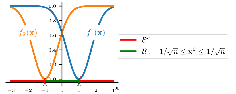
We use the problem introduced by Fonseca (1995) to show the advantage of EPO Search (Algorithm 1) over competing approaches: LS, PMTL and CS (where (1) is solved). This problem consists of two non-convex objective functions (30) that are to be minimized over ; Figure 5 shows the functions for . In this problem, the set of PO solutions is a subset of the hyper-box defined in (31), where denotes the partial ordering induced by the positive cone in the solution space. Note that for , we have as shown in Figure 5. We evaluate each MOO algorithm in two scenarios, when the initialization is: (a) inside this hyper-box, i.e., , and (b) outside this hyper-box, i.e., . The latter is more difficult, especially when the EPO is far from the initialization . For instance, in Figure 5, if the desired optimal is and the initialization is at , the iterate has to escape the minimum of objective , i.e., , to reach . In other words, without ascending in , it is not possible to reach from in a continuous trajectory, i.e., using a gradient-based iterative algorithm. Each algorithm is tested with four weight vectors, spread uniformly over the first quadrant. The number of iterations, step size, and random initializations are the same for all algorithms.
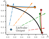
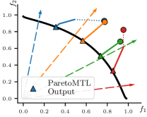
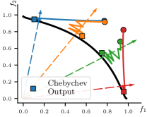
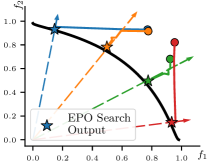
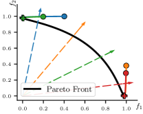

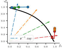
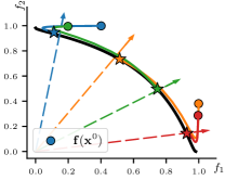
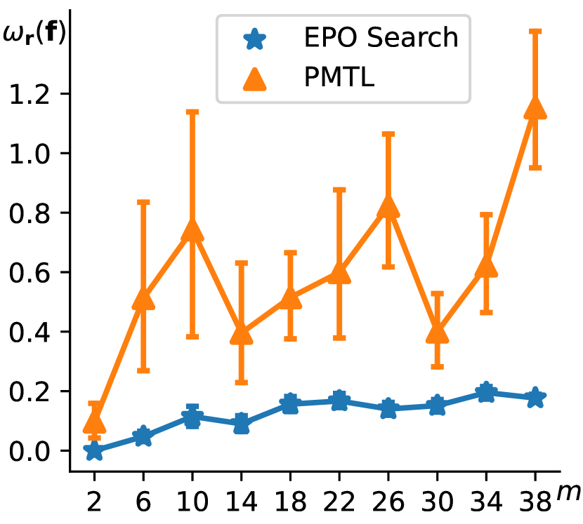
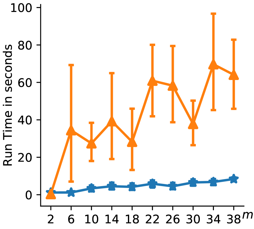
Figure 6 shows the results. LS does not reach any of the EPO solutions, owing to its theoretical limitations for non-convex MOO problems. In its phase 1, PMTL enters the vicinity of the EPO, and in phase 2 it descends to the PF, although not exactly to the goal. However, PMTL converges to the PF only when initialized near the EPO, and diverges otherwise, e.g., in the green and yellow trajectories of Figure 6(b) when . The CS method theoretically has the EPO as its solution, but in practice, when an iterative procedure is used with a step size, it oscillates around the ray (Figure 6(a)), without reaching the goal exactly because only one objective (with the maximum relative value (1)) is considered in each iteration. Although the oscillations could be reduced with a smaller step size, it would demand more number of iterations to reach the EPO. Using only one objective becomes more problematic if it’s gradient magnitude vanishes. For instance, the green and yellow trajectory in Figure 6(b) does not make substantial progress. This is similar to the d scenario in Figure 5 discussed above, i.e., if and , only will be considered whose gradient is close to zero. On the other hand, EPO search reaches very close to all the EPO solutions. Unlike CS, it uses a linear combination of all the objectives’ gradients. As a result, it descends along the ray without oscillations. Moreover, the ability to ascend enables EPO Search to escape the minima of less preferred objectives in Figure 6(b) making it robust to initialization.
We extend the above example to create objectives functions and compare PMTL with EPO Search, with respect to their scalability. The objective functions are defined as , for , where the entries of are sampled uniformly in . For every , we run both the algorithms for different (dimension of solution space), randomly sampled within and . We randomly select a weight vector in for every pair. In addition PMTL requires reference vectors; for a fair comparison, we provide (maximum number of constraints in EPO search in this problem) reference vectors, which are again randomly selected in .
We use from Lagrange identity (12) as a measure of the quality of the solutions found. For every pair, both the algorithms were run for iterations with equal step size. Figure 7(a) and 7(b) show the quality and run time, respectively, for different number of objectives (). Compared to PMTL, EPO search scales better with increasing number of objectives and produces better quality solutions.
5.2 Pareto front tracing by EPO Search: Illustrations on benchmark problems
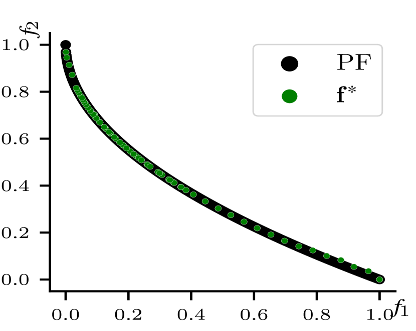
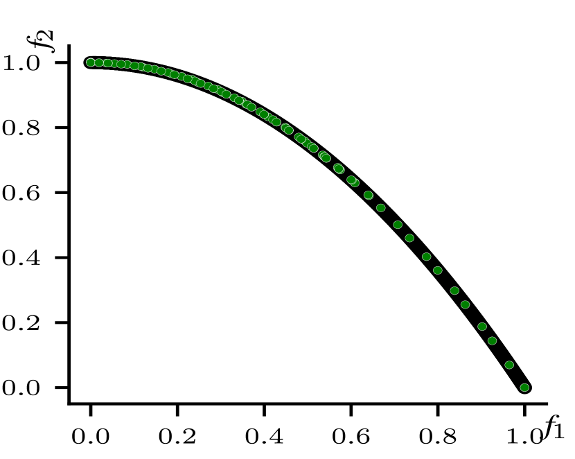
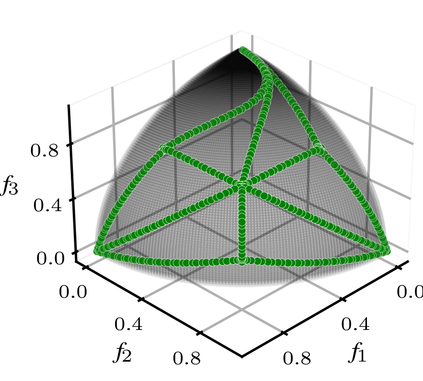
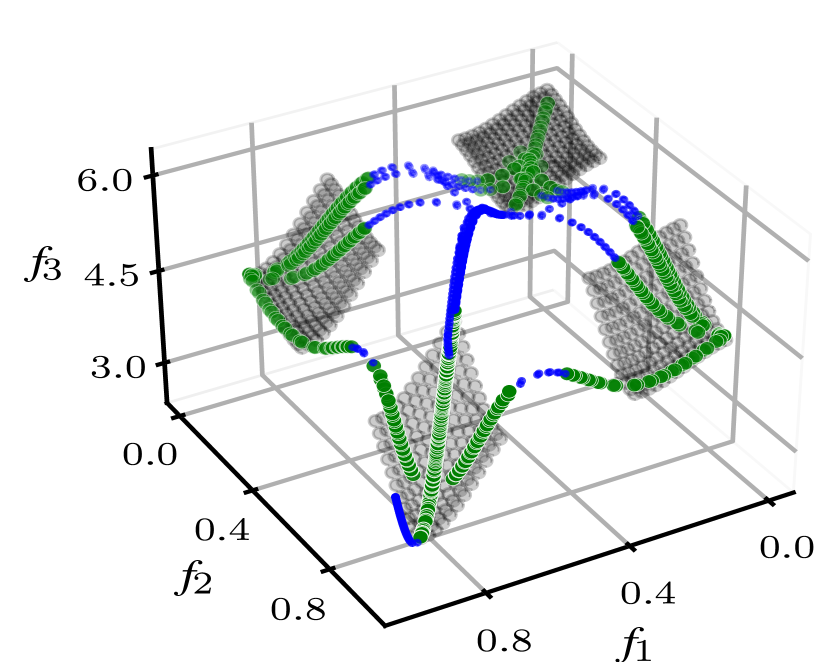
We show the tracing ability of EPO Search Algorithm 2 on 6 benchmark MOO problems: ZDT1, ZDT2, ZDT3 (Zitzler et al. 2000), DTLZ2 and DTLZ7 (Deb et al. 2005), and TNK (Tanaka et al. 1995). We use PESA (Stanojević and Glover 2020) (see §4.1) to generate rays.
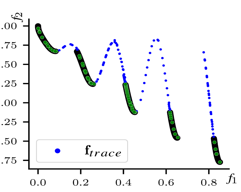
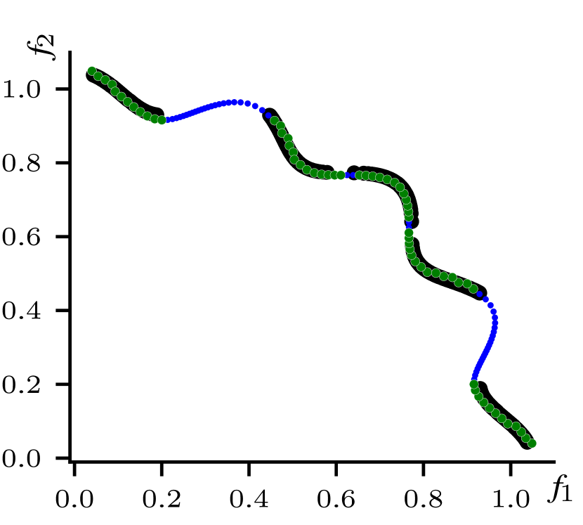
The ZDT series of problems minimize two objectives: and , where , for ZDT1, for ZDT2 and for ZDT3. The argument is bounded as for . Figures 8(a), 8(b) and 8(c) show the results. In these results, the depth of PESA procedure is 1 for ZDT1 and ZDT2, and 2 for ZDT3. Note that ZDT3 has a disconnected PF, but its boundary of attainable objective vectors is connected. Therefore, while tracing, EPO Search connects the disconnected segments of the PF by tracing the boundary through . This is made possible due to the controlled gradient ascent within EPO Search. In the TNK problem, . The two objectives to minimize are and with bounds and the inequality constraints , and . It has a discontinuous PF. Figure 8(d) shows the tracing result for this problem.
The DTLZ series of problems have more than two objectives to minimize. Let the last variables of be denoted as . The objective functions in DTLZ2 are defined as
with . In DTLZ7, the first objective vectors are for . The last objective is defined as , where , and . Figures 8(e) and 8(f) shows the tracing results for DTLZ problems. Note that DTLZ7 has disconnected PF but has a connected boundary of attainable objective vectors . Therefore, akin to ZDT3, here also EPO Search connects the PFs while tracing. For clarity of presentation, we show the tracing results for rays generated up to a recursion depth of 3 in PESA.
5.3 Evaluation of PESA-EPO for Pareto front approximation
We numerically compare the efficacy of PESA-EPO Algorithm 3 in PF approximation with PESA-CS and two state-of-the-art algorithms: CTAEA (Li et al. 2019), and PESA-TDM (Stanojević and Glover 2020). CTAEA (Constrained Two-Archive Evolutionary Algorithm) is an evolutionary algorithm, whereas PESA-TDM (Pattern Efficient Search Algorithm with Targeted Directional Model) is a gradient-based algorithm. Empirically, CTAEA has been found to outperform C-MOEA/D, C-NSGA-III (Jain and Deb 2013), C-MOEA/DD (Li et al. 2014), I-DBEA (Asafuddoula et al. 2014) and CMOEA (Woldesenbet et al. 2009); and the performance of PESA-TDM was found to be similar or better than NSGA-II (Deb et al. 2002), MOEA/DDE (Li and Zhang 2009), MOEA/D-AWA (Qi et al. 2014), MOEA/D-UD1 and MOEA/D-UD2 (Zhang et al. 2015). In PESA-CS, CS (by solving (1)) is used instead of TDM.
To evaluate how closely the obtained solutions approximate the PF, we use Inverted Generational Distance (IGD) (Coello Coello and Reyes Sierra 2004), defined in (32), where the ground truth PF is a finely discretized set of solutions from the actual PF , and is the set of points found by an algorithm. Ground truth PFs for the problems (§5.2) were obtained from Durillo et al. (2010), Durillo and Nebro (2014). IGD values and time of execution for all the methods are shown in Table 1.
| MOO Problems | Metrics | CTAEA | PESA-TDM | PESA-CS | PESA-EPO |
|---|---|---|---|---|---|
| ZDT1 () | IGD | 0.0426 | 0.0088 | 0.0095 | 0.0016 |
| Times (s) | 4.01 | 1.71 | 2.1 | 1.38 | |
| ZDT2 () | IGD | 0.0404 | 0.0051 | 0.0059 | 0.0016 |
| Times (s) | 4.05 | 9.93 | 11.75 | 1.14 | |
| ZDT3 () | IGD | 0.0572 | 0.0217 | 0.062 | 0.0027 |
| Times (s) | 4.08 | 20.23 | 38.75 | 1.85 | |
| TNK () | IGD | 0.0922 | 0.0069 | 0.0117 | 0.0061 |
| Times (s) | 1.64 | 0.61 | 6.48 | 0.83 | |
| DTLZ2 () | IGD | 0.0269 | 0.0681 | 0.1214 | 0.0307 |
| Times (s) | 221.77 | 40.38 | 68.13 | 2.9 | |
| DTLZ7 () | IGD | 0.0369 | 0.0439 | 0.1532 | 0.0384 |
| Times (s) | 60.49 | 41.74 | 48.16 | 2.32 |
| (32) | ||||
The results indicate that PESA-EPO is able to efficiently (lower time of execution) achieve close approximation to the PF (lower IGD). CTAEA uses a decomposition technique similar to PMTL (§2.3 and Appendix D.3). Its computational complexity grows exponentially with the number of objectives, as seen in our experiment as well. The time required to reach an IGD value of same scale as that of the competing algorithms is significantly more in DTLZ2 and DTLZ7, where , as compared to the other bi-objective problems. PESA-TDM is efficient and suitable when the dimension of solution space is low: in TNK, it achieves as good an approximation as PESA-EPO with lesser execution time. Although PESA-CS is similar to PESA-TDM, it requires more samples of weight vectors from the PESA recursions (see §4.1) since CS stagnates for some weights and does not reach the PF, thereby requiring more time to achieve similar level of IGD values as that of PESA-TDM. For high-dimensional solution spaces both PESA-TDM and PESA-CS are inefficient because, for every new weight vector in PESA, they have to solve an optimization problem starting from a random initialization. On the other hand, PESA-EPO uses a previously obtained EPO as an initialization to solve the next problem. Moreover, the points in the trajectory of this optimization are PO solutions. As a result, PESA-EPO efficiently achieves very good performance.
5.4 Evaluation of GP-EPO for preference elicitation
To evaluate an interactive PE algorithm, we measure the decrease in regret with the number of queries to the DM. The regret at the query is defined as the difference between the oracle utility and the incumbent, i.e., the best solution so far:


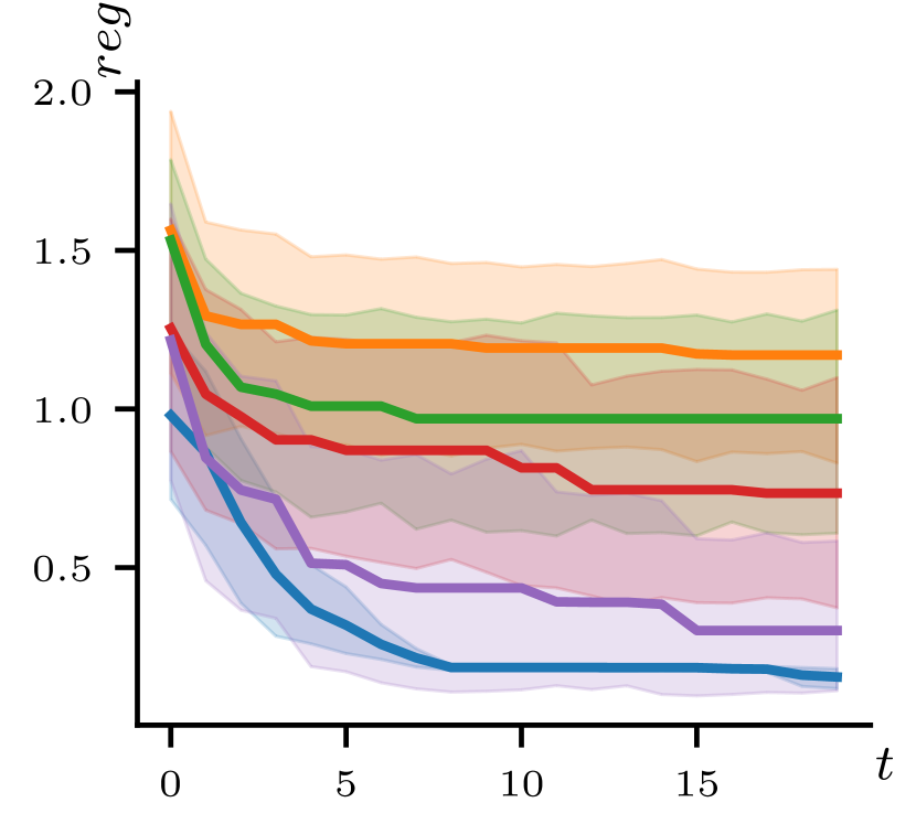

We use the same 6 MOO problems described in §5.2 to evaluate GP-EPO. Following Ozbey and Karwan (2014), we use the Chebyshev utility function (which is unknown to the PE algorithm) to simulate a virtual DM that compares between two alternatives. Previous GP-based PE methods (Chin et al. 2018, Zintgraf et al. 2018, Roijers et al. 2021), differ from GP-EPO in the use of (8) with a discrete set of points (that could, e.g., be generated by a PF approximator like PESA-EPO). However, we use a stronger baseline by using the ground truth PFs of the 6 MOO problems as the discrete set. We randomly choose (without replacement) of the ground truth PF for the PE, and call it BL-. For all the PE methods, we use Gaussian kernel and expected improvement as the acquisition function. We run each method for 10 trials, and in each trial, the utility of the virtual DM (parameters of Chebyshev utility) are decided randomly, to test the methods for different oracle solutions. We compare the decrement in their regrets for up to 20 queries.
The results are shown in Figure 9. We observe that for every MOO problem, GP-EPO surpasses the baseline methods that use up to 90 % of the ground truth PO solutions. Among the baseline results, the regret consistently decreases with increase in size of the discrete set . This decrement in regret is more prominent when the PE problem (7) is non-convex, i.e., when the MOO has a non-convex range in the objective space. E.g., in the ZDT family, ZDT1 has a convex MOO problem, and the difference between regret curves for 70%, 80% and 90% are not significant. Whereas, ZDT2 and ZDT3 have non-convex , which, we conjecture, makes the difference between regret curves significant. Note that, in the baseline approach, similar to the state-of-the-art for GP-based PE, the discrete set of PO solutions has to be obtained before Bayesian optimization (8) can start for PE. However, in practice, it is unclear as to how many PO solutions would suffice to reach a desired level of regret. From the baseline results it is clear that if the discrete set represents the PF at a coarser resolution, then the regret may not go lower than a certain level, since there may not be enough samples closer to the oracle solution. Whereas, in GP-EPO, only two PO solutions are required a priory for the first query to start PE. We obtain the first PO solution by solving for and the second one by solving for a random . Since the Bayesian optimization (29) is over a continuous domain, GP-EPO can probe the PF virtually at infinite resolution. Therefore, unlike the baseline approach, its regret keeps decreasing without saturating after few initial queries.
5.5 Evaluation of EPO Search for Multi-Task Learning on Real Data
We demonstrate the efficacy of EPO Search for MTL in three applications from diverse domains. We discuss application 1 in the following and the other two in Appendix F.
5.5.1 Personalized Medicine and Pharmacogenomics.
We consider three drug-related tasks from different stages of drug discovery and development, summarized in Table 2. We use data from multiple publicly available databases summarized in Table 4. More details of these tasks and datasets used are in Appendix E. These tasks model the effects of drugs in hierarchically increasing levels of complexity. Drug-target (DT) prediction models the effect of drugs on specific genes (targets); drug response (DR) prediction models the effect of drugs on cancer cells (or a cancer patient with a given genomic profile); Drug side effect (DS) prediction models the side effects of drugs on patients. Hence, we expect DT to benefit less from auxiliary signal of the other two tasks. Among the three tasks, DR is the most challenging because data for relatively fewer drugs are available and we expect DR to benefit the most from MTL.
MTL Model. A standard deep neural MTL architecture (DNN-MTL) is used, as illustrated in Figure 10, where feature representations of each of the four entities, viz., drug, target gene, cancer cell, and disease, are used. These features are first passed through separate feed-forward neural networks (FNN) to get their corresponding embeddings, then the task-specific embedding pairs are concatenated and passed through task-specific FNN predictors for the final outputs – classifiers for DT and DS, and regressor for DR. The model is trained with binary cross entropy loss for DT and DS, and mean squared error loss for DR. Each embedding FNN has one hidden layer of neurons, and each predictor FNN has two hidden layers, neurons followed by , totaling parameters for the entire model. Each sub-network is associated with its parameters denoted by where represent embedding, classification and regression respectively; represent each of the tasks and represents the shared drug-related features. In this MTL-DNN model, the network parameters of drug embedding FNN are shared for all the tasks, making it a suitable testbed for MOO training. The dimensions of input feature and embeddings are given in Table 4. Additional details are in Appendix E.
| Prediction Task | Problem | Inputs | Output(s) | |
|---|---|---|---|---|
| 1 | Drug Target (DT) | Binary Classification | Drug , Gene | 1: is a target of , 0: otherwise |
| 2a | Drug Response (DR) | Regression | Drug , Genomic Profile | Drug efficacy of on |
| 2b | Drug Response (DR) | Ranking | Drug list, Genomic Profile | Top- most effective drugs for |
| 3 | Drug Side Effect (DS) | Binary Classification | Drug , Disease | 1: is a side effect of , 0: otherwise |
| Task | Dataset | No. of Drugs | No. Sample pairs | |
| Training | Test | |||
| Drug Target | STITCH | 16K | 627596 | 263032 |
| DrugBank | 6K | 158708 | 75820 | |
| Repur | 4K | 80080 | 39798 | |
| Drug Response | GDSC | 235 | 128004 | 62849 |
| CCLE | 483 | 212516 | 109529 | |
| Drug Side-effect | SIDER | 1.4K | 524395 | 259471 |
| OFFSIDE | 2.2K | 550888 | 278807 | |
| Drug | Gene-Target | Cell-line | Disease | |
|---|---|---|---|---|
| Features | 300 | 800 | 300 | 300 |
| Embeddings | 128 | 128 | 128 | 128 |
Experiment Setting. In each dataset, 1/3rd of the drugs are randomly chosen to create a held-out test set; the remaining 2/3rd of the drugs are used for training. The total number of samples used in train and test sets are given in Table 4. For classification tasks, DT and DS, performance is measured using Area Under ROC curve (AUROC) and Area Under PR curve (AUPRC). For DR, we use two metrics: Mean Squared Error (MSE) and the ranking metric Normalized Discounted Cumulative Gain (NDCG@10) to judge how well the top most effective drugs are predicted for a cancer patient and thus evaluate the model from the perspective of clinical use.
We compare EPO Search with LS and CS. In each of these methods, we determine the trade-off between DR and DS by having a higher priority (100) for one and lower priority for the other (1). DT plays a supporting role for both these tasks as it is the most specific task and we expect it to benefit the least from MTL. So, we keep its priority fixed at (10) for all scenarios. We report the results for the model trained with a maximum priority for the corresponding task. In addition, we use Single Task Learning (STL) as a baseline, where each task-specific network of the MTL-DNN model is trained with data for each task independently. For every priority setting, training for each method is repeated over 5 runs to randomize over model initialization and mini-batch formation, and the mean and standard deviations of the metrics are reported. We use paired test to determine statistical significance at 0.05 significance level. If a method is pair-wise better than all the other methods, then we mark the result with an asterisk. Results are shown in Table 5.
| Task | Dataset | Metric | Algorithms | |||
|---|---|---|---|---|---|---|
| STL | CS | LS | EPO Search | |||
| Drug Target (DT) | STITCH | AUROC | 94.90 0.18 | 95.17 0.40 | 95.08 0.20 | 95.55 0.27∗ |
| AUPRC | 79.36 0.46 | 79.14 0.99 | 79.55 0.66 | 79.86 0.61 | ||
| DrugBank | AUROC | 91.95 0.34 | 92.41 0.24 | 91.88 0.25 | 92.66 0.21∗ | |
| AUPRC | 66.35 0.60 | 66.42 0.99 | 65.76 0.67 | 67.52 0.59∗ | ||
| Repur | AUROC | 90.80 0.53 | 91.35 0.18 | 90.45 0.29 | 91.16 0.31 | |
| AUPRC | 64.54 1.59 | 64.97 0.15 | 64.34 1.09 | 65.15 1.13 | ||
| Drug Response (DR) | GDSC | MSE | 1.030 0.02 | 1.012 0.05 | 1.029 0.02 | 0.965 0.02 |
| NDCG@10 | 52.69 2.15 | 54.55 1.55 | 53.05 2.11 | 56.62 1.84∗ | ||
| CCLE | MSE | 0.854 0.02 | 0.857 0.04 | 0.862 0.02 | 0.827 0.04 | |
| NDCG@10 | 48.70 0.94 | 50.28 1.31 | 47.80 1.15 | 53.67 0.90∗ | ||
| Drug Side-effect (DS) | SIDER | AUROC | 77.39 0.20 | 77.37 0.15 | 77.46 0.14 | 78.60 0.33∗ |
| AUPRC | 39.02 1.25 | 40.01 1.33 | 39.58 1.07 | 41.29 1.25∗ | ||
| OFFSIDE | AUROC | 80.10 0.19 | 80.53 0.20 | 80.14 0.14 | 81.23 0.33∗ | |
| AUPRC | 61.43 0.69 | 62.00 0.45 | 61.23 0.37 | 62.93 0.58∗ | ||
Results. First, we observe that in almost all cases, CS and EPO Search perform better than STL, which demonstrates the advantages of EPO solutions for MTL, and DR, which is a more challenging problem, is most benefited. Although LS uses gradient information from all the tasks, it fails to consistently perform better than STL as the priorities are disproportionate among the tasks. This can be attributed to the non-convexity of loss surface, for which LS gravitates towards an extreme PO solution, as illustrated in §5.1. STL can be considered as a MOO method that finds an extreme solution corresponding to one task only. We observe that in some cases, e.g. CCLE, LS performs even worse than STL. In these cases, the simple weighted sum strategy inhibits LS from reaching the PF as close as STL does. Near an extreme solution the gradient directions are opposing and a fixed weight gradient combination reduces the magnitude of the search direction, especially when the gradient magnitude of a less preferred task is high. A reduced magnitude in the search direction decreases the magnitude of resulting network update. With fixed learning rate and number of iterations, update magnitude finally determines proximity to the PF.
CS benefits from MTL by amortizing its usage of gradient information from different tasks over many iteration, but only after reaching the ray, as illustrated in §5.1. Before that it behaves like STL, since only the maximum relative objective (1) is minimized. On the other hand, EPO Search adaptively combines the gradient information in every iteration and moves closer to the EPO solution of the training losses as compared to CS. This is reflected, through better performance with respect to the evaluation metrics, on the test data as well.
For DS, EPO Search outperforms other methods in both datasets and both metrics. In DR, EPO search outperforms other methods in the clinically important metric, NDCG@10, in both datasets. In DT, EPO search outperforms other methods in the DrugBank dataset, on both metrics and in the STITCH dataset on AUROC. Overall, in 13 out of 14 cases, EPO Search has the best average performance, and in 10 out of the 13 cases, the improvement is statistically significant.
5.5.2 Summary of Results on Real Data.
In Appendix F we evaluate EPO Search in two other applications. The first, from hydrometeorology, consists of predicting river flow at 8 sites in the Mississippi river network – a problem with 8 regression tasks. The second, from e-commerce, consists of 2 classification problems, predicting the category of multiple fashion product images simultaneously. In all cases, our results demonstrate the advantages of MTL over learning for each task independently, and the superior performance of EPO-Search over competing MTL methods.
6 Conclusion
In this paper we present new first-order iterative algorithms to find EPO solutions, for both unconstrained and constrained non-convex MOO problems. EPO Search is designed for problems with high-dimensional solution spaces where it is computationally more efficient than popular evolutionary algorithms. From a random initialization, EPO Search converges to an EPO solution or, if an EPO solution does not exist, to the closest PO solution. We prove its convergence and empirically demonstrate that our approach addresses the shortcomings of oscillations and premature stagnation in previous methods using the min-max formulation of (1). Similar to existing gradient descent methods, the convergence rate of EPO Search is sub-linear when moving from a random point to a Pareto stationary point. Interestingly, we show that the convergence rate, from any PO point to the EPO is linear under mild conditions. The literature on CS has methods to obtain EPO solutions, but without convergence guarantees; while the literature on gradient-based MOO methods presents convergence guarantees but only to reach arbitrary PO solutions. EPO Search offers both: a robust iteration strategy to reach the desired EPO and with convergence guarantees.
A direct application of the improved MOO through EPO Search is seen in MTL. Most previous MTL models use LS to combine task-specific priorities and losses. While CS is more suitable for non-convex loss functions, if the the min-max formulation of (1) is used, learning is dominated by the task with highest priority and the influence of other tasks is either low or absent. In contrast, EPO Search uses a combination of gradients of all tasks in every iteration and can escape the minima of low priority objectives through controlled ascent which improves learning and makes it robust to initialization. The per-iteration complexity of EPO Search remains linear in the gradient dimensions (similar to the best previous methods that neither use input priorities nor allow constraints on parameters) enabling its use for deep MTL networks. We demonstrate the superior performance of EPO Search over competing approaches in MTL on synthetic and real datasets. EPO Search allows us to prioritize training for tasks that are more challenging while leveraging the MTL framework which enables shared learning from other datasets and tasks. We observe this in our own experiments where drug response prediction, which has the least number of drugs for training, benefits from collective learning of drug side effects and drug targets.
When initialized on the PF, EPO search can systematically trace the PF to reach an EPO solution, with a theoretically guaranteed linear rate of convergence. This unique ability makes it a computationally efficient alternative in use cases that require traversing the PF from one EPO solution to another. We investigate two such use cases in MCDM and develop new algorithms based on EPO Search. First we develop PESA-EPO for a posteriori MCDM where multiple EPO solutions can be used to approximate a PF. On benchmark datasets, PESA-EPO is faster than competing alternatives, without compromising on the approximation quality, because it does not require multiple optimizer calls and does not stop prematurely at PF discontinuities. Second, we develop GP-EPO for PE in interactive MCDM where we also address two limitations of previous GP-based PE methods by developing a new formulation. We leverage EPO Search to efficiently find PO solutions given a ray in in GP-EPO that samples in a lower-dimensional space , instead of the higher-dimensional solution space which previous methods use; moreover, this obviates the need to explicitly model monotonicity constraints. Numerical experiments on benchmark problems confirm the advantages of GP-EPO in terms of improved regret with very few queries to the DM.
Future Directions.
The key idea of our convergence rate proof is to compose non-convex objective functions with a well behaved function that satisfies the PL inequality (the proportionality gauges in our case) whose minima lie close to the desired PO. This enables reaching the vicinity of the desired solution at a linear rate. This idea may be utilized in other contexts, e.g., to solve non-convex SOO by (a) additional (convex or non-convex) objective functions and (b) a function satisfying PL inequality that, upon composition, models a solution in a convex neighbourhood of the global optimal of the original non-convex objective. A limitation of EPO Search, that may be addressed in future work, is that the tracing procedure can approximate the entire PF starting from the extreme solutions only if the set is connected, i.e., there are paths connecting the discontinuous segments of the PF. Note that this is the case for disconnected PFs, in problems ZDT3, TNK and DTLZ7 in §5.3. If is not connected, e.g. in MOO problems of Wang et al. (2019), then more initial seed points are required in each connected component of . For instance, techniques to add relevant non-extreme seed points by detecting discontinuities in the PF during tracing in EPO Search could be investigated. Regularization on the network parameters, through our extension to handle constraints, may be empirically evaluated for MTL in future work. Finally, methods to adaptively find the best priorities for an MTL model may be explored in future work. A possibility is to adapt our method GP-EPO such that the DM’s role is replaced by validation dataset performance to compare solutions.
References
- Adams and Pagano (2016) Adams TE, Pagano T (2016) Flood forecasting: A global perspective (Academic Press).
- Angur et al. (1996) Angur MG, Lotfi V, Sarkis J (1996) A hybrid conjoint measurement and bi-criteria model for a two group negotiation problem. Socio-Economic Planning Sciences 30(3):195–206.
- Armbruster and Delage (2015) Armbruster B, Delage E (2015) Decision making under uncertainty when preference information is incomplete. Management Science 61(1):111–128.
- Asafuddoula et al. (2014) Asafuddoula M, Ray T, Sarker R (2014) A decomposition-based evolutionary algorithm for many objective optimization. IEEE Transactions on Evolutionary Computation 19(3):445–460.
- Beninger (2018) Beninger P (2018) Pharmacovigilance: an overview. Clinical Therapeutics 40(12):1991–2004.
- Boyd and Vandenberghe (2004) Boyd S, Vandenberghe L (2004) Vector optimization. Convex Optimization, chapter 4.7, 174–187 (Cambridge University Press).
- Cai et al. (2013) Cai X, Wang G, Zhang Z (2013) Complexity analysis and numerical implementation of primal-dual interior-point methods for convex quadratic optimization based on a finite barrier. Numerical Algorithms 62(2):289–306.
- Caruana (1997) Caruana R (1997) Multitask learning. Machine Learning 28(1):41–75.
- Chang et al. (2019) Chang FJ, Hsu K, Chang LC (2019) Flood Forecasting using Machine Learning Methods (MDPI).
- Chen et al. (2020) Chen H, Cheng F, Li J (2020) idrug: Integration of drug repositioning and drug-target prediction via cross-network embedding. PLoS Computational Biology 16(7):e1008040.
- Cheng et al. (2021) Cheng WH, Song S, Chen CY, Hidayati SC, Liu J (2021) Fashion meets computer vision: A survey. ACM Computing Surveys (CSUR) 54(4):1–41.
- Chin et al. (2018) Chin R, Manzie C, Ira A, Nesic D, Shames I (2018) Gaussian processes with monotonicity constraints for preference learning from pairwise comparisons. 2018 IEEE Conference on Decision and Control (CDC), 1150–1155.
- Chu and Ghahramani (2005) Chu W, Ghahramani Z (2005) Preference learning with Gaussian processes. Proceedings of the 22nd International Conference on Machine Learning, 137–144, ICML ’05.
- Coello Coello and Reyes Sierra (2004) Coello Coello CA, Reyes Sierra M (2004) A study of the parallelization of a coevolutionary multi-objective evolutionary algorithm. MICAI 2004: Advances in Artificial Intelligence, 688–697 (Berlin, Heidelberg: Springer Berlin Heidelberg).
- Coloma et al. (2013) Coloma PM, Avillach P, Salvo F, Schuemie MJ, Ferrajolo C, Pariente A, Fourrier-Réglat A, Molokhia M, Patadia V, van der Lei J, et al. (2013) A reference standard for evaluation of methods for drug safety signal detection using electronic healthcare record databases. Drug Safety 36(1):13–23.
- Corsello et al. (2017) Corsello SM, Bittker JA, Liu Z, Gould J, McCarren P, Hirschman JE, Johnston SE, Vrcic A, Wong B, Khan M, Asiedu J, Narayan R, Mader CC, Subramanian A, Golub TR (2017) The drug repurposing hub: a next-generation drug library and information resource. Nature Medicine 23(4):405–408.
- Das and Dennis (1997) Das I, Dennis JE (1997) A closer look at drawbacks of minimizing weighted sums of objectives for pareto set generation in multicriteria optimization problems. Structural Optimization 14(1):63–69.
- Das and Dennis (1998) Das I, Dennis JE (1998) Normal-boundary intersection: A new method for generating the Pareto surface in nonlinear multicriteria optimization problems. SIAM Journal on Optimization 8(3):631–657.
- Daulton et al. (2022) Daulton S, Eriksson D, Balandat M, Bakshy E (2022) Multi-objective Bayesian optimization over high-dimensional search spaces. Uncertainty in Artificial Intelligence, 507–517 (PMLR).
- Deb and Jain (2014) Deb K, Jain H (2014) An evolutionary many-objective optimization algorithm using reference-point-based nondominated sorting approach, part i: Solving problems with box constraints. IEEE Transactions on Evolutionary Computation 18(4):577–601.
- Deb et al. (2002) Deb K, Pratap A, Agarwal S, Meyarivan T (2002) A fast and elitist multiobjective genetic algorithm: NSGA-II. IEEE Transactions on Evolutionary Computation 6(2):182–197.
- Deb et al. (2005) Deb K, Thiele L, Laumanns M, Zitzler E (2005) Scalable test problems for evolutionary multiobjective optimization. Abraham A, Jain L, Goldberg R, eds., Evolutionary Multiobjective Optimization: Theoretical Advances and Applications, 105–145 (Springer London).
- Deisenroth et al. (2013) Deisenroth MP, Fox D, Rasmussen CE (2013) Gaussian processes for data-efficient learning in robotics and control. IEEE Transactions on Pattern Analysis and Machine Intelligence 37(2):408–423.
- Deldjoo et al. (2022) Deldjoo Y, Nazary F, Ramisa A, Mcauley J, Pellegrini G, Bellogin A, Di Noia T (2022) A review of modern fashion recommender systems. arXiv preprint arXiv:2202.02757.
- Dell and Karwan (1990) Dell RF, Karwan MH (1990) An interactive MCDM weight space reduction method utilizing a Tchebycheff utility function. Naval Research Logistics (NRL) 37(2):263–277.
- Désidéri (2012) Désidéri JA (2012) Multiple-gradient descent algorithm (MGDA) for multiobjective optimization. Comptes Rendus Mathematique 350(5-6):313–318.
- DiMasi et al. (2016) DiMasi JA, Grabowski HG, Hansen RW (2016) Innovation in the pharmaceutical industry: new estimates of r&d costs. Journal of Health Economics 47:20–33.
- Durillo and Nebro (2014) Durillo JJ, Nebro AJ (2014) jMetal: Metaheuristic algorithms in Java. http://jmetal.sourceforge.net/problems.html.
- Durillo et al. (2010) Durillo JJ, Nebro AJ, Alba E (2010) The jMetal framework for multi-objective optimization: Design and architecture. IEEE Congress on Evolutionary Computation, 1–8.
- Elahi and Qi (2020) Elahi M, Qi L (2020) Fashion recommender systems in cold start. Fashion Recommender Systems, 3–21 (Springer).
- Emmerich and Deutz (2018) Emmerich MT, Deutz AH (2018) A tutorial on multiobjective optimization: fundamentals and evolutionary methods. Natural Computing 17(3):585–609.
- Eric et al. (2007) Eric B, Freitas N, Ghosh A (2007) Active preference learning with discrete choice data. Advances in Neural Information Processing Systems 20.
- Fishburn (1968) Fishburn PC (1968) Utility theory. Management Science 14(5):335–378.
- Fliege and Svaiter (2000) Fliege J, Svaiter BF (2000) Steepest descent methods for multicriteria optimization. Mathematical Methods of Operations Research 51(3):479–494.
- Fliege and Vaz (2016) Fliege J, Vaz AIF (2016) A method for constrained multiobjective optimization based on SQP techniques. SIAM Journal on Optimization 26(4):2091–2119.
- Fonseca (1995) Fonseca CMMd (1995) Multiobjective genetic algorithms with application to control engineering problems. Ph.D. thesis, University of Sheffield.
- Forgas (1995) Forgas JP (1995) Mood and judgment: The affect infusion model (AIM). Psychological Bulletin 117(1):39–66.
- Gandibleux (2002) Gandibleux X (2002) Multiple Criteria Optimization: state of the art annotated bibliographic surveys, volume 52 of International Series in Operations Research & Management Science (Springer US).
- Gembicki and Haimes (1975) Gembicki F, Haimes Y (1975) Approach to performance and sensitivity multiobjective optimization: The goal attainment method. IEEE Transactions on Automatic Control 20:769–771.
- Goodfellow et al. (2016) Goodfellow I, Bengio Y, Courville A (2016) Deep Learning (MIT Press).
- Greco et al. (2010) Greco S, Matarazzo B, Slowiński R (2010) Interactive evolutionary multiobjective optimization using dominance-based rough set approach. IEEE Congress on Evolutionary Computation, 1–8 (IEEE).
- Hardt (1975) Hardt RM (1975) Topological properties of subanalytic sets. Transactions of the American Mathematical Society 211:57–70.
- Haskell et al. (2018) Haskell WB, Huang W, Xu H (2018) Preference elicitation and robust optimization with multi-attribute quasi-concave choice functions. arXiv preprint arXiv:1805.06632.
- Hillermeier (2001) Hillermeier C (2001) Nonlinear Multiobjective Optimization: A Generalized Homotopy Approach, volume 135 of International Series of Numerical Mathematics (Birkhaüser Verlag).
- Huang et al. (2012) Huang SM, Lertora JJ, Atkinson Jr AJ (2012) Principles of Clinical Pharmacology (Academic Press).
- Hwang et al. (1979) Hwang CL, Masud ASM, Hwang CL, Masud ASM (1979) Methods for multiple objective decision making. Multiple Objective Decision Making—Methods and Applications: A State-of-the-Art Survey 21–283.
- Ismail-Yahaya and Messac (2002) Ismail-Yahaya A, Messac A (2002) Effective generation of the Pareto frontier: The normalized normal constraint method. 43rd AIAA/ASME/ASCE/AHS/ASC Structures, Structural Dynamics, and Materials Conference.
- Jain and Deb (2013) Jain H, Deb K (2013) An evolutionary many-objective optimization algorithm using reference-point based nondominated sorting approach, part II: Handling constraints and extending to an adaptive approach. IEEE Transactions on Evolutionary Computation 18(4):602–622.
- Jain (2007) Jain V (2007) On Cauchy’s bound for zeros of a polynomial. Bulletin mathématique de la Société des Sciences Mathématiques de Roumanie 50 (98)(3):273–279.
- Jiang et al. (2021) Jiang Y, Rensi SE, Wang S, Altman RB (2021) Drugorchestra: Jointly predicting drug response, targets, and side effects via deep multi-task learning. 25th International Conference on Research in Computational Molecular Biology.
- Jing et al. (2019) Jing R, Wang M, Zhang Z, Liu J, Liang H, Meng C, Shah N, Li N, Zhao Y (2019) Comparative study of posteriori decision-making methods when designing building integrated energy systems with multi-objectives. Energy and Buildings 194:123–139.
- Jones (2001) Jones DR (2001) A taxonomy of global optimization methods based on response surfaces. Journal of Global Optimization 21(4):345–383.
- Kaliszewski (1995) Kaliszewski I (1995) A theorem on nonconvex functions and its application to vector optimization. European Journal of Operational Research 80(2):439–445.
- Karimi et al. (2016) Karimi H, Nutini J, Schmidt M (2016) Linear convergence of gradient and proximal-gradient methods under the Polyak-Lojasiewicz condition. Frasconi P, Landwehr N, Manco G, Vreeken J, eds., Machine Learning and Knowledge Discovery in Databases, 795–811 (Cham: Springer International Publishing).
- Keeney et al. (1993) Keeney RL, Raiffa H, Meyer RF (1993) Decisions with multiple objectives: preferences and value trade-offs (Cambridge university press).
- Kiriiri et al. (2020) Kiriiri GK, Njogu PM, Mwangi AN (2020) Exploring different approaches to improve the success of drug discovery and development projects: a review. Future Journal of Pharmaceutical Sciences 6(1):1–12.
- Köksalan and Wallenius (2012) Köksalan M, Wallenius J (2012) Multiple criteria decision making: foundations and some approaches. New Directions in Informatics, Optimization, Logistics, and Production, 171–183 (INFORMS).
- Köksalan and Sagala (1995) Köksalan MM, Sagala PN (1995) Interactive approaches for discrete alternative multiple criteria decision making with monotone utility functions. Management Science 41(7):1158–1171.
- Korhonen et al. (1984) Korhonen P, Wallenius J, Zionts S (1984) Solving the discrete multiple criteria problem using convex cones. Management Science 30(11):1336–1345.
- Kuhn et al. (2016) Kuhn M, Letunic I, Jensen LJ, Bork P (2016) The SIDER database of drugs and side effects. Nucleic Acids Res. 44(D1):D1075–9.
- LeCun et al. (1998) LeCun Y, Bottou L, Bengio Y, Haffner P (1998) Gradient-based learning applied to document recognition. Proceedings of the IEEE 86(11):2278–2324.
- Li and Zhang (2009) Li H, Zhang Q (2009) Multiobjective optimization problems with complicated Pareto sets, MOEA/D and NSGA-II. IEEE Transactions on Evolutionary Computation 13(2):284–302.
- Li et al. (2019) Li K, Chen R, Fu G, Yao X (2019) Two-archive evolutionary algorithm for constrained multiobjective optimization. IEEE Transactions on Evolutionary Computation 23(2):303–315.
- Li et al. (2014) Li K, Deb K, Zhang Q, Kwong S (2014) An evolutionary many-objective optimization algorithm based on dominance and decomposition. IEEE Transactions on Evolutionary Computation 19(5):694–716.
- Lin et al. (2020) Lin X, Yang Z, Zhang Q, Kwong S (2020) Controllable Pareto multi-task learning. arXiv preprint arXiv:2010.06313 .
- Lin et al. (2019) Lin X, Zhen HL, Li Z, Zhang QF, Kwong S (2019) Pareto multi-task learning. Advances in Neural Information Processing Systems, volume 32 (Curran Associates, Inc.).
- Luenberger (1997) Luenberger DG (1997) Optimization by Vector Space Methods (USA: John Wiley & Sons, Inc.).
- Luenberger and Ye (2008) Luenberger DG, Ye Y (2008) Primal Methods, 359–400 (New York, NY: Springer US).
- Luque et al. (2007) Luque M, Caballero R, Molina J, Ruiz F (2007) Equivalent information for multiobjective interactive procedures. Management Science 53(1):125–134.
- Ma et al. (2021) Ma J, Fong SH, Luo Y, Bakkenist CJ, Shen JP, Mourragui S, Wessels LF, Hafner M, Sharan R, Peng J, et al. (2021) Few-shot learning creates predictive models of drug response that translate from high-throughput screens to individual patients. Nature Cancer 2(2):233–244.
- Marler and Arora (2004) Marler RT, Arora JS (2004) Survey of multi-objective optimization methods for engineering. Structural and Multidisciplinary Optimization 26(6):369–395.
- Miettinen (1998) Miettinen K (1998) Nonlinear Multiobjective Optimization, volume 12 of International Series in Operations Research & Management Science (Springer US).
- Močkus (1975) Močkus J (1975) On Bayesian methods for seeking the extremum. Marchuk GI, ed., Optimization Techniques IFIP Technical Conference Novosibirsk, July 1–7, 1974, 400–404 (Berlin, Heidelberg: Springer Berlin Heidelberg).
- Nesterov (2004) Nesterov Y (2004) Nonlinear Optimization, 1–50 (Boston, MA: Springer US).
- Ng (2015) Ng R (2015) Drugs: from discovery to approval (John Wiley & Sons).
- NOAA National Centers for Environmental Information (2022) NOAA National Centers for Environmental Information (2022) U.S. Billion-Dollar Weather and Climate Disasters.
- Nocedal and Wright (2006) Nocedal J, Wright SJ (2006) Theory of constrained optimization. Numerical Optimization, chapter 12.2, 315–320 (New York, NY, USA: Springer), second edition.
- Ozbey and Karwan (2014) Ozbey O, Karwan MH (2014) An interactive approach for multicriteria decision making using a Tchebycheff utility function approximation. Journal of Multi-Criteria Decision Analysis 21(3-4):153–172.
- Oztas and Erdem (2021) Oztas GZ, Erdem S (2021) Framework selection for developing optimization algorithms: assessing preferences by conjoint analysis and best–worst method. Soft Computing 25(5):3831–3848.
- Pascoletti and Serafini (1984) Pascoletti A, Serafini P (1984) Scalarizing vector optimization problems. Journal of Optimization Theory and Applications 42(4):499–524.
- Polyak (1963) Polyak B (1963) Gradient methods for the minimisation of functionals. USSR Computational Mathematics and Mathematical Physics 3(4):864–878.
- Qi et al. (2014) Qi Y, Ma X, Liu F, Jiao L, Sun J, Wu J (2014) MOEA/D with Adaptive Weight Adjustment. Evolutionary Computation 22(2):231–264.
- Rao (2010) Rao VR (2010) Conjoint Analysis (John Wiley & Sons, Ltd).
- Rasmussen and Williams (2004) Rasmussen CE, Williams CK (2004) Gaussian processes in machine learning. Lecture Notes in Computer Science 3176:63–71.
- Rees et al. (2016) Rees MG, Seashore-Ludlow B, Cheah JH, Adams DJ, Price EV, Gill S, Javaid S, Coletti ME, Jones VL, Bodycombe NE, Soule CK, Alexander B, Li A, Montgomery P, Kotz JD, Hon CSY, Munoz B, Liefeld T, Dančík V, Haber DA, Clish CB, Bittker JA, Palmer M, Wagner BK, Clemons PA, Shamji AF, Schreiber SL (2016) Correlating chemical sensitivity and basal gene expression reveals mechanism of action. Nat. Chem. Biol. 12(2):109–116.
- Reeves and MacLeod (1999) Reeves GR, MacLeod KR (1999) Some experiments in Tchebycheff-based approaches for interactive multiple objective decision making. Computers & Operations Research 26(13):1311–1321.
- Roijers et al. (2021) Roijers DM, Zintgraf LM, Libin P, Reymond M, Bargiacchi E, Nowé A (2021) Interactive multi-objective reinforcement learning in multi-armed bandits with Gaussian process utility models. Hutter F, Kersting K, Lijffijt J, Valera I, eds., Machine Learning and Knowledge Discovery in Databases, 463–478 (Cham: Springer International Publishing).
- Ruder (2017) Ruder S (2017) An overview of multi-task learning in deep neural networks. arXiv preprint arXiv:1706.05098.
- Sabour et al. (2017) Sabour S, Frosst N, Hinton GE (2017) Dynamic routing between capsules. Advances in Neural Information Processing Systems, volume 30 (Curran Associates, Inc.).
- Schenone et al. (2013) Schenone M, Dančík V, Wagner BK, Clemons PA (2013) Target identification and mechanism of action in chemical biology and drug discovery. Nature Chemical Biology 9(4):232–240.
- Sener and Koltun (2018) Sener O, Koltun V (2018) Multi-task learning as multi-objective optimization. Advances in Neural Information Processing Systems, volume 31 (Curran Associates, Inc.).
- Senft et al. (2017) Senft D, Leiserson MD, Ruppin E, Ze’ev AR (2017) Precision oncology: the road ahead. Trends in Molecular Medicine 23(10):874–898.
- Shahriari et al. (2016) Shahriari B, Swersky K, Wang Z, Adams RP, De Freitas N (2016) Taking the human out of the loop: A review of Bayesian optimization. Proceedings of the IEEE 104(1):148–175.
- Shukla (2007) Shukla PK (2007) On the normal boundary intersection method for generation of efficient front. Shi Y, van Albada GD, Dongarra J, Sloot PMA, eds., Computational Science – ICCS 2007, 310–317 (Springer Berlin Heidelberg).
- Siddiqui et al. (2012) Siddiqui S, Azarm S, Gabriel SA (2012) On improving normal boundary intersection method for generation of Pareto frontier. Structural and Multidisciplinary Optimization 46(6):839–852.
- Snoek et al. (2012) Snoek J, Larochelle H, Adams RP (2012) Practical Bayesian optimization of machine learning algorithms. Advances in Neural nformation Processing Systems, 2951–2959.
- Spyromitros-Xioufis et al. (2016) Spyromitros-Xioufis E, Tsoumakas G, Groves W, Vlahavas I (2016) Multi-target regression via input space expansion: treating targets as inputs. Machine Learning 104(1):55–98.
- Stanojević and Glover (2020) Stanojević B, Glover F (2020) A new approach to generate pattern-efficient sets of non-dominated vectors for multi-objective optimization. Information Sciences 530:22–42.
- Steuer (1989) Steuer RE (1989) The Tchebycheff procedure of interactive multiple objective programming. Karpak B, Zionts S, eds., Multiple Criteria Decision Making and Risk Analysis Using Microcomputers (Springer).
- Steuer et al. (1993) Steuer RE, Silverman J, Whisman AW (1993) A combined Tchebycheff/aspiration criterion vector interactive multiobjective programming procedure. Management Science 39(10):1255–1260.
- Stewart et al. (2008) Stewart T, Bandte O, Braun H, Chakraborti N, Ehrgott M, Göbelt M, Jin Y, Nakayama H, Poles S, Stefano DD (2008) Real-world applications of multiobjective optimization. Multiobjective Optimization 285–327.
- Szklarczyk et al. (2016) Szklarczyk D, Santos A, von Mering C, Jensen LJ, Bork P, Kuhn M (2016) STITCH 5: augmenting protein-chemical interaction networks with tissue and affinity data. Nucleic Acids Res. 44(D1):D380–4.
- Tanabe et al. (2022) Tanabe H, Fukuda EH, Yamashita N (2022) Convergence rates analysis of a multiobjective proximal gradient method. Optimization Letters .
- Tanaka et al. (1995) Tanaka M, Watanabe H, Furukawa Y, Tanino T (1995) GA-based decision support system for multicriteria optimization. 1995 IEEE International Conference on Systems, Man and Cybernetics. Intelligent Systems for the 21st Century, volume 2, 1556–1561.
- Tatonetti et al. (2012) Tatonetti NP, Ye PP, Daneshjou R, Altman RB (2012) Data-driven prediction of drug effects and interactions. Sci. Transl. Med. 4(125):125ra31.
- Tesauro (1988) Tesauro G (1988) Connectionist learning of expert preferences by comparison training. Touretzky D, ed., Advances in Neural Information Processing Systems, volume 1 (Morgan-Kaufmann).
- Vamathevan et al. (2019) Vamathevan J, Clark D, Czodrowski P, Dunham I, Ferran E, Lee G, Li B, Madabhushi A, Shah P, Spitzer M, et al. (2019) Applications of machine learning in drug discovery and development. Nature Reviews Drug Discovery 18(6):463–477.
- Vayanos et al. (2020) Vayanos P, Ye Y, McElfresh D, Dickerson J, Rice E (2020) Robust active preference elicitation. arXiv preprint arXiv:2003.01899.
- Ventola (2018) Ventola CL (2018) Big data and pharmacovigilance: data mining for adverse drug events and interactions. Pharmacy and Therapeutics 43(6):340.
- Vieira et al. (2012) Vieira DAG, Takahashi RHC, Saldanha RR (2012) Multicriteria optimization with a multiobjective golden section line search. Mathematical Programming 131(1):131–161.
- Wallenius et al. (2008) Wallenius J, Fishburn PC, Zionts S, Dyer JS, Steuer RE, Deb K (2008) Multiple criteria decision making, multiattribute utility theory: Recent accomplishments and what lies ahead. Management Science 54(7):1336–1349.
- Wang et al. (2019) Wang Y, Yu J, Yang S, Jiang S, Zhao S (2019) Evolutionary dynamic constrained optimization: Test suite construction and algorithm comparisons. Swarm and Evolutionary Computation 50(6):972–986.
- Watanabe et al. (2018) Watanabe JH, McInnis T, Hirsch JD (2018) Cost of prescription drug–related morbidity and mortality. Annals of Pharmacotherapy 52(9):829–837.
- Wiecek et al. (2016) Wiecek MM, Ehrgott M, Engau A (2016) Continuous multiobjective programming. Multiple Criteria Decision Analysis: State of the Art Surveys (Springer).
- Wierzbicki (1986) Wierzbicki AP (1986) On the completeness and constructiveness of parametric characterizations to vector optimization problems. Operations-Research-Spektrum 8(2):73–87.
- Wishart et al. (2018) Wishart DS, Feunang YD, Guo AC, Lo EJ, Marcu A, Grant JR, Sajed T, Johnson D, Li C, Sayeeda Z, Assempour N, Iynkkaran I, Liu Y, Maciejewski A, Gale N, Wilson A, Chin L, Cummings R, Le D, Pon A, Knox C, Wilson M (2018) DrugBank 5.0: a major update to the DrugBank database for 2018. Nucleic Acids Res. 46(D1):D1074–D1082.
- Woldesenbet et al. (2009) Woldesenbet YG, Yen GG, Tessema BG (2009) Constraint handling in multiobjective evolutionary optimization. IEEE Transactions on Evolutionary Computation 13(3):514–525.
- Xiao et al. (2017) Xiao H, Rasul K, Vollgraf R (2017) Fashion-MNIST: a novel image dataset for benchmarking machine learning algorithms. arXiv preprint arXiv:1708.07747.
- Yang and Shami (2020) Yang L, Shami A (2020) On hyperparameter optimization of machine learning algorithms: Theory and practice. Neurocomputing 415:295–316.
- Yang et al. (2013) Yang W, Soares J, Greninger P, Edelman EJ, Lightfoot H, Forbes S, Bindal N, Beare D, Smith JA, Thompson IR, Ramaswamy S, Futreal PA, Haber DA, Stratton MR, Benes C, McDermott U, Garnett MJ (2013) Genomics of drug sensitivity in cancer (GDSC): a resource for therapeutic biomarker discovery in cancer cells. Nucleic Acids Res. 41(Database issue):D955–61.
- Zhang et al. (2018) Zhang C, Tan KC, Lee LH, Gao L (2018) Adjust weight vectors in MOEA/D for bi-objective optimization problems with discontinuous Pareto fronts. Soft Comput. 22(12):3997–4012.
- Zhang et al. (2021) Zhang M, Huang K, Lv Y (2021) A wide neighborhood arc-search interior-point algorithm for convex quadratic programming with box constraints and linear constraints. Optimization and Engineering 1–21.
- Zhang and Li (2007) Zhang Q, Li H (2007) MOEA/D: A multiobjective evolutionary algorithm based on decomposition. IEEE Transactions on Evolutionary Computation 11(6):712–731.
- Zhang et al. (2008) Zhang Q, Zhou A, Jin Y (2008) RM-MEDA: A regularity model-based multiobjective estimation of distribution algorithm. IEEE Transactions on Evolutionary Computation 12(1):41–63.
- Zhang and Yang (2021) Zhang Y, Yang Q (2021) A survey on multi-task learning. IEEE Transactions on Knowledge and Data Engineering .
- Zhang et al. (2015) Zhang Y, Yang R, Zuo J, Jing X (2015) Enhancing MOEA/D with uniform population initialization, weight vector design and adjustment using uniform design. Journal of Systems Engineering and Electronics 26(5):1010–1022.
- Zintgraf et al. (2018) Zintgraf LM, Roijers DM, Linders S, Jonker CM, Nowé A (2018) Ordered preference elicitation strategies for supporting multi-objective decision making. Proceedings of the 17th International Conference on Autonomous Agents and MultiAgent Systems, 1477–1485, AAMAS ’18 (Richland, SC: International Foundation for Autonomous Agents and Multiagent Systems).
- Zionts and Wallenius (1976) Zionts S, Wallenius J (1976) An interactive programming method for solving the multiple criteria problem. Management Science 22(6):652–663.
- Zitzler et al. (2000) Zitzler E, Deb K, Thiele L (2000) Comparison of multiobjective evolutionary algorithms: Empirical results. Evolutionary Computation 8(2):173–195.
Appendix
| Notations | Description |
|---|---|
| , and | number of variables in the solution space, and number of objectives |
| valued objective function, or a vector in | |
| dimensional simplex | |
| preference vector, and its point-wise inverse | |
| a Pareto Optimal solution, an Exact Pareto Optimal solution w.r.t | |
| solution and its objective vector at iteration | |
| lower and upper bounds (box constraint) on solution variable: | |
| Projection function that brings inside the box constraints element-wise | |
| number of inequality and equality constraints | |
| valued inequality and valued equality constraints | |
| number of active inequality and equality constraints | |
| Jacobians of objectives, active inequality and and equality constraints | |
| Set of feasible solutions, and range of valued objective function | |
| Boundaries of domain and range of respectively | |
| Interior of domain and range of respectively | |
| Set of Pareto optimal solutions, and Exact Pareto Optimal solutions w.r.t | |
| Tangent plane/cone, set of feasible directions, descent directions at | |
| a general search direction, non-dominating search direction | |
| coefficients for gradients of objectives, active inequality and equality constraints | |
| A measure of proportionality of w.r.t. | |
| or simply | Anchor direction at point w.r.t. preference |
| maximum relative value of objectives: | |
| index set of objectives with maximum relative value | |
| set of attainable objective vectors dominated by and | |
| set of attainable objective vectors with measure of proportionality | |
| discrete sets of preference vectors at start, and after 3 recursion in PESA | |
| mean, kernel and acquisition functions of a Gassian Process | |
| function that maps a point in the Simplex to the PF | |
| Pairwise comparison data constructed from the queries to the DM. | |
| The discrete set of solutions present in the dataset |
Appendix A Proportionality of Vectors and Balancing Direction
A.1 Proportionality Gauge from KL Divergence
One possible approach to measure the proportionality between and is through KL divergence between the normalized vectors of and , i.e. the uniform distribution:
| (33) |
where is the normalization of a vector . This satisfies both conditions 1 and 2 of a proportionality gauge. Figure 3(c) shows the corresponding in case of objectives and a particular weight vector. Its anchor direction is scale invariant to :
| (34) |
Notice that, unless all are equal, the anchor elements are non-negative for some objectives and negative for the rest. As a result, if we move against the search direction in Theorem 3, we will be descending for the objectives with and ascending for the other objectives, since . This is further clarified by analyzing the relation between and .
claimklaf The anchor direction in (34) is always orthogonal to the objective vector : .
However, this anchoring direction (34) does not move the objective vectors to the ray in the shortest possible path. The shortest path between and the ray should lie on the hyperplane containing both these vectors. So, in order for to be on the shortest path, a necessary condition is should lie in the span of and . This does not happen in anchoring direction of (34) as shown in the Figure 3(c) and 3(d). The curved trajectory deviates from the .
A.2 Comparison of Proportionality Gauges
Among the three options discussed above, we use CSZ inequality and Lagrange’s identity based proportionality gauges as their anchoring directions satisfy the PL inequality (see Lemma 3.6), which we leverage in §3.6 to prove linear convergence in Theorem 3. It is non-trivial to design a scaling factor for the KL divergence based anchor (34) such that satisfies the PL inequality in Lemma (3.6). Therefore, we do not use this in our development. We use Lagrange identity based anchoring direction when the initialization is not on the PF, in order to reach the ray through the shortest path in lesser number of iterations as compared to the CSZ inequality based anchor. However, when the initialization is on the PF, in order to escape the local PO solution, we use the CSZ inequality based anchoring direction. Table 7 summarizes their properties.
Appendix B Constrained Multi-Objective Optimization
Our approach for Constrained MOO is similar to that of Fliege and Vaz (2016), where the descent based method (discussed in §2.1.1) is used to handle constraints. But their method cannot obtain EPO solutions specific to an like ours, which is facilitated by both ascent and descent. The constrained domain or Feasible Solution Set is defined as
| (38) |
where & are domain boundaries for each variable, are differentiable inequality constraints, and are differentiable equality constraints.
We check for the infeasibility of boundary, equality and inequality constraints in each iteration. If violates any of the boundary constraints, we project element-wise to , to constrain them to remain within the bounds, where
| (39) |
Let the number of active inequality constraints be , making total active constraints, since the equality constraints are always active. Without loss of generality, let the active inequality constraints be for . Then the cone of first order feasible directions at against which we can move to obtain is given by
| (40) |
where and . When there is no active constraint it is the same as the tangent plane: . Note, the tangent plane is the set of directions that keeps the next iterate in the feasible region:
| (41) |
When there are active constraints, the tangent plane becomes a tangent cone as certain directions would lead out of the feasible region . However, the first order feasible directions may not be equal to always. The tangent cone is unique and depends on the geometrical property of at . But, the cone is not unique and depends on the algebraic specification of the constraints (see (Nocedal and Wright 2006)[Ch 12.2]) through the functions s and s. E.g., although the constraints and are algebraically different (at , whereas ), they are geometrically the same constraints. At a boundary point , if the gradients of the active constraint function are linearly independent (Nocedal and Wright 2006). This is called as Linear Independence Constraint Qualification (LICQ). Therefore, to make same as the tangent cone , and render the conditions in (40) useful, we assume the LICQ to be satisfied at every .
B.1 Constrained EPO Search for Random Initialization
We modify the QP (17) into
| (42a) | ||||
| s.t. | (42b) | |||
| (42c) | ||||
| (42d) | ||||
where is as defined in (17c). This is similar to the gradient projection strategy for constrained SOO (Luenberger and Ye 2008). The search direction , can be considered as the projection of the search direction obtained from QP (17) onto the set (40). However in practice, at a boundary point , the projected gradient may not guarantee to move the iterate to , the interior of , unless the step size is infinitesimal. Therefore, in our implementation we modify (42b) to for a whenever the inequality constraint is violated . Similarly, we modify (42c) to if and if for a . We increase the values of if , and increase further as , until the iterate becomes feasible.
Similar to the unconstrained MOO case, this QP also satisfies the following two Lemmas by construction: {restatable}lemmadndbalconst If is a non-PO regular point of the differentiable vector function in a balance mode, i.e. , then the non-dominating direction obtained from QP (42) makes
-
1.
non-negative angles with the gradients of maximum relative objectives: (17c),
-
2.
a positive angle with the balancing anchor direction (13) in the objective space: .
lemmadnddesconst If is a non-PO regular point of the differentiable vector function in a descent mode, i.e. , then the non-dominating direction obtained from QP (42) makes a non-negative angle with every gradient, , and a positive angle with at least one gradient.
B.2 Constrained EPO Search for Tracing the Pareto Front from
We modify the QP (22) into
| (43a) | ||||
| s.t. | (43b) | |||
| (43c) | ||||
| (43d) | ||||
| and | (43e) | |||
where is the CSZ inequality based anchor direction (11). Note that we have excluded the constraint (42d) associated to objectives of . Because, if the objective vector is (approximately) on the Pareto front, then some objectives with highest relative value () may require a further increase in their value to move towards an EPO solution.
Pareto Criticality for constrained MOO:
At a point , the set of descent directions is given by At a local Pareto optimal point there does not exist any non-zero feasible descent direction, i.e. . Note that, if there are no active constraints at , . A necessary condition to check if a point is Pareto optimal, i.e., , is given by Pareto Criticality:
| (44) |
where and are the Jacobians of inequality and equality constraints. This is formulated by extending the KKT conditions to a multi-objective setup (see (Hillermeier 2001)[Ch 4]). When there are no active constraints at an optimal point , the Pareto criticality condition in (44) reduces to for some .
Penetration Assumption:
We introduce the penetration assumption to guarantee non-convergence at a non-EPO point when there are active constraints, i.e, and . We assume there exists an such that for all , where . In other words, an infinitesimal step along the direction of objective vector starting from will take it to the interior of . We call this as penetrates .
theoremdndnc Let such that, if then it is a regular Pareto optimal solution, and if then it is a regular point of and penetrates . Then, at , the non-dominating direction found by the QP (43) with Cauchy-Schwarz anchor (11) is if and only if . We consider the penetration assumption to be mild because, when the range set is dimensional and its boundary is dimensional, almost all points in that violate the penetration assumption are not Pareto optimal, not even locally. Figure 11 illustrates a scenario where it is violated. If a point violates penetration along with the points in any of its dimensional (relative) open neighbourhoods in , then penetrates , and thus is dominated by for some small . The assumption of dimensional boundary is fairly general since it is similar to the assumption of regular Pareto optimal in the unconstrained case.
Appendix C Proofs of Lemmas and Theorems
C.1 Proportionality Gauge
*
Proof.
We first prove (9a) by considering as a function of , . Taylor’s expansion of this function can be written with the Peano’s form of remainder as
| (45) |
where is the transpose of gradient , and the asymptotic notation little- represents a function that approaches faster than . In particular, for every , there exists an such that
| (46) |
Applying chain rule of differentiation on , we get
We know that is non-negative from the statement of the Lemma 3. Therefore, when positive, we treat as , and use the property of as mentioned in (46) to conclude there exists a step size such that
| (47) |
and hence ; equality holds when . That proves (9a).
In the following Lemma C.1, we prove a property of scale invariant balancing anchor direction, that will be used in the proves of Theorem 3. {restatable}lemmafagtra If is such that the anchoring direction is scale invariant to , i.e., for all , where then
| (50) |
Proof.
We use the second property of stated in 2, i.e. increases monotonically with . In other words, , for . At , the chain rule reveals
| (51) | ||||
| (52) |
We apply the scale invariance property of the anchor direction to the preference vector in (52):
| (53) | ||||
| (54) |
Applying to (54), we get . Therefore, applying to (54), we get , i.e. must not be positive. ∎
*
Proof.
*
Proof.
The proof is apparent from the formula of the anchoring direction (11). ∎
*
Proof.
The proof is apparent from the formula of the anchoring direction (13). ∎
*
Proof.
We expand , where , as
where . We use the fact that , and further expand as
In the inner summation we can now add the term for as and write the above expression as
The double summation in the numerator can be written as the inner product of a symmetric and a skew-symmetric matrix which is equal to . ∎
C.2 EPO Search for Unconstrained MOO
*
Proof.
We denote the subset of all possible directions in the tangent space of an objective vector , which is constrained due to restrictions on the coefficients , as
| (55) |
where is defined in (16). We split the proof for two scenarios: 1) and 2) .
In the first scenario, the the minimum value is achieved for the objective (17a) with , , and hence
| (56) |
We can invert due to the regularity assumption. Note that for all when and are not proportional. This can be deduced from its formula in (13) as follows
-
1.
for all .
-
2.
. If not true, then Claim 3.1.2 is contradicted for any .
-
3.
, for any . definition of in (13).
-
4.
1, 2 and 3 for all .
As a result, the constraint (17b) is inactive when , because . Now, with we can invoke Theorem 3, and that proves Lemma 17 for the first scenario.
In the second scenario, i.e., , the satisfies the first property, i.e., for all , due to the constraint (17b). We prove the second property, i.e., , by contradiction. Let be the optimum of the QP (17), such that . Then the optimal cost value of (17a) can be written as
| (57) |
However, this is a contradiction due to the following counterexample that yields a lesser value of the cost than . The satisfies the constraints (17b) as proven for the previous scenario, and the cost value of this coefficient is .
That concludes the proof. ∎
*
Proof.
In the descent mode the anchor direction is . Similar to the proof of Lemma 17, we split this proof into two scenarios: 1) and 2) , where is defined in (55).
For the first scenario, the proof is similar to that of Lemma 17, where . And the constraint (17b) is redundant, since for all . There exist at least one such that , and therefore makes positive angle with the corresponding gradient. The point is a utopia point in our formulation and cannot be attained.
Beyond Regularity Assumption: Lemmas 17 and 17 can be true even without the full rank assumption of . In particular, when is in the interior of the domain, (56) can be satisfied if the anchor direction , the column space of .
*
Proof.
We prove for unconstrained MOO using Lemmas 17 and 17 for the QP (17). However, the same proof holds true for constrained MOO by using Lemmas B.1 and B.1 for the QP (42).
We divide the proof into descent mode and balance mode.
From Lemma 17, in the descent mode, i.e. , The QP in (17), produces a search direction that makes non-negative angle with each gradient, i.e. for all . As a result, by applying the Taylor’s expansion with Peano form of remainder to each along with the property of little-o notation, one can deduce that for every there exists a step size such that for all . If we choose , then for all , we have
| ( definition of in (18)) | (58) | ||||
| ( definition of in (3.4.1)) | (59) | ||||
Next, we consider the balance mode. Let be the index set for descending objectives and for ascending ones. So, there exists an for all such that
for all . Let , and , where is the maximum step size one can take so that . Then for all , and
Lemma 17 ensures that . If all the other objectives in also satisfy
then can be used as the step size as it is. If this is not the case, i.e. there exists some such that
then continuity of the objective functions ensures that there must exists some such that
So choosing we finally get
for all . ∎
*
Proof.
*
Proof.
The necessity prove is trivial; because if , then the CSZ inequality based anchor direction in (11) is , resulting a coefficient from the QP (22), and search direction.
For the sufficiency, we prove the contra-positive: if , then . When , is non-zero. For a non-zero , the in the QP (22) will be zero only when lies in the null space of . But if , then ; because is orthogonal to the CSZ inequality-based anchor from Claim 3.1.1, and from the regularity condition. If is in the column space of then there exists a such that , which makes a descent direction. This is a contradiction, as no descent direction should exist at the Pareto optimal . In fact, the eigenvector of corresponding to its Null space must be an all positive vector like the objective vector in order to exclude all possible descent direction from the . Note, the eigenvectors of are orthogonal to each other. Therefore and will not be zero from the QP (22), hence . ∎
Beyond Regularity Assumption: In general, this Theorem is true even without the regularity assumptions when the orthogonal projection of the CSZ inequality-based anchor (11) onto the hyperplane is non-zero.
Issue of Lagrange Identity based Balancing Anchor Direction: The anchor direction in (13) is not orthogonal to the objective vector . Therefore, in a corner case, the anchor direction may be very close to the as shown in Figure 12(a). Therefore its projection on to will vanish. However, CSZ inequality-based anchor (11) mitigates this issue as shown in Figure 12(b). Note, the set defined in (19) is different for both the proportionality gauges. In practice, although this extreme scenario may not arise, but the projection of on to will have a lesser magnitude in Lagrange identity based anchor as compared to that of KL divergence based anchor.
*
Proof.
First we prove for the Cauchy-Schwarz inequality based and .
| (60) | ||||||
| (61) | ||||||
| (62) | ||||||
| (63) | ||||||
| (64) | ||||||
| (65) | ||||||
| (66) | ||||||
*
Proof.
We use a property of Lipschitz smooth functions. If be a scalar valued function whose gradient is smooth with Lipschitz , then (see Lemma 1.2.3 in Nesterov (2004))
| (72) |
From Lipschitz smoothness Assumptions 2, we can write the following inequality for :
| (73) |
where . Similarly, with , Jacobian at as , stepsize , and
| (74) | ||||
| (75) |
is obtained from solving the QP (17) or (22) in the balance mode, we can write the following inequalities for :
| (76) | ||||||
| (77) | ||||||
| (78) | ||||||
| (79) | ||||||
| (80) |
where has all ones. If no subscript is mentioned explicitly then means norm. In (78), we have applied Cauchy-Schwarz inequality.
Next, we upper bound the term in (73) as
| (81) | |||||
| (82) | |||||
| (83) | |||||
| (84) | |||||
| (85) | |||||
| (86) |
In (81), we use the right (left) inequality in (80) if is positive (negative) for . In (84), the factors and are as given in the statement of the theorem. The step (81)(82) is similar to (77)(79). The step (84)(85) because, by construction, the solution of QP in (17) or (22) gives .
Similarly, we upper bound the term in (73) as
| (87) | ||||||
| (88) | ||||||
| (89) |
Finally, we can rewrite (73) as
| (90) | ||||||
| (91) | ||||||
| (92) | ||||||
| (93) | ||||||
where the polynomial has the coefficients as given in the statement of the theorem. The ideal stepsize that minimizes is given by the positive root of
| (94) |
The in the statement of the theorem is such that . We obtain this lower bound using the following properties of a polynomial.
-
(i)
Cauchy’s upper bound (Jain 2007) for all the absolute roots of a polynomial , i.e., , is given by
-
(ii)
is the lower bound for all the absolute roots of polynomial .
Finally, applying Properties (i) and (ii) on the polynomial (94), we get the as given in the statement of the theorem.
The iteration complexity, i.e., the maximum number of iterations until which is given by
| (95) | ||||||
| (96) | ||||||
| (97) | ||||||
| (98) | ||||||
| (99) | ||||||
∎
Lemma 1.
Proof.
We can write
| (101) |
where is the angle between the anchor direction and the direction . In this prove we find lower bound for . Note, if (defined in (55)), then (e.g., see proof of Lemma 17), which is an upper bound for . Therefore, we only consider for .
First, we lower bound . The maximum possible value of ; it occurs when , which results in , where . This is a feasible solution even for the constrained balance mode in the QP (17) as proven in Lemma 17. Here, the residue is aligned with . The minimum possible value of (or the maximum angle between and ) will occur when the residue is orthogonal to . In other words, and are the base and hypotenuse of a right triangle. Therefore,
| (102) | |||||
| (103) | |||||
Next, we lower bound . To minimize the quadratic cost , the vector must lie on the boundary of , resulting in
| (104) |
We first lower bound when :
| (105) | ||||||
| (106) | ||||||
| (107) | ||||||
| (108) | ||||||
| (109) | ||||||
| (110) |
Now, we consider the case . From the definition of (25), we know that the lowest singular value vanishes as approaches the PF. As a result, the corresponding singular vector (eigenvector of ) turns into the null space of as approaches222Note, similar to the singular values, the singular vectors are also smooth w.r.t. variations in due to the smoothness of Jacobian . the PF, because according to Assumption 3, the second singular value does not vanish in . In other words, the column space of becomes equal to the columns space of . The QP (22) is used in such cases. Its balancing anchor direction as proven in Theorem 3.5.1, where we deduced that must be an all positive vector like the descending anchor direction . Moreover, since and are orthogonal (see Claim 3.1.1), to minimize , gets projected onto the in . Therefore, instead of in (106) and (107), the second singular value is applicable, which results in
| (111) | ||||||
| (112) | ||||||
| (113) | ||||||
| (114) |
Therefore, for any we can write
| (115) |
Finally, we can lower bound the inner product as
| (116) | ||||||
| (117) | ||||||
| (118) | ||||||
| (119) |
∎
C.3 EPO Search for Constrained MOO
*
Proof.
The statement is true by construction of the QP (42). ∎
*
Proof.
The statement is true by construction of the QP (42). ∎
*
Appendix D Useful variations in EPO Search
In practice, for high-dimensional solution spaces , e.g. DNN parameters, we use a fixed step size instead of adaptively deciding by line search. So, for proper movement in the objective space, we introduce few variations in the EPO search algorithm.
D.1 Momentum in Anchor While Tracing
While tracing the Pareto front, i.e. starting from a Pareto optimal , we use the Cauchy-Schwarz anchor direction (11), which is always perpendicular to the objective vector (see Claim 3.1.1). The first order change in the objective space created by the search direction found from QP (43) is . This change is same as the orthogonal projection of onto the cone . When the Pareto front is connected, at any point on the Pareto front, , so the magnitude of is significant enough to move the iterate with a small step size. But when, the Pareto front is disconnected, e.g. ZDT3 in Figure 8(c), and the iterate is at a boundary point outside the Pareto front, , then , and the magnitude of its projection may not be enough to propel the iterate ahead with a small step size. The movements in objective slows down. To mitigate this we use a momentum term in the anchor,
| (120) |
and use in the QP. Using this anchor if the next iterate is dominated by the current one, i.e. , then we conclude that , and don’t enter the descent mode in the subsequent iterations and only operate in the balance mode. As soon as a non-dominated iterate is found, i.e. , we resume alternating the modes of operation.
D.1.1 Importance of Alternating Mode of Operation While Tracing.
It is important to use the descent mode of operation in every other iteration to keep the iterate close to the Pareto front, especially in case of convex objectives. Otherwise the trajectory will drift away from the Pareto front. This is shown in Figure 13 for ZDT1 problem.
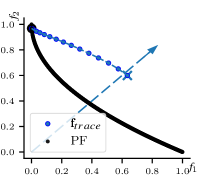
D.2 Restricting Trajectory in Descent Mode When not Tracing
When reaching the EPO solution starting from an arbitrary initialization, ideally the algorithm should enter the descent mode only when the iterate reaches exactly onto the ray. Because, when , the anchor direction of descent becomes , and the iterates descend along the to reach the EPO solution. But achieving while using a fixed step size is less likely. Therefore we perform a descent mode operation whenever the objective vector lies in the cone
| (121) |
for a small . As a result, the descending anchor direction, and hence the first order change in objective space , will no longer be aligned with the ray. This causes oscillations around the ray while descending, as shown in Figure 14(a). To mitigate this, we add the following equality constraint to the QP (15) for unconstrained MOO and (42) for constrained MOO:
| (122) |
where is the normalized vector, and is the identity matrix. This constraint ensures that the movement in the objective space will be aligned with ray. We apply this equality constraint only when there are no active constraints, i.e. . The restriction in (122) makes the trajectory of descent mode non-oscillatory as shown in Figure 14(b). The objective functions used in Figure 14 is described in section 5.1.
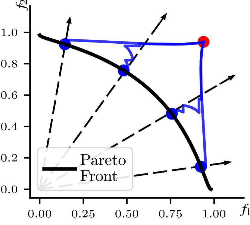
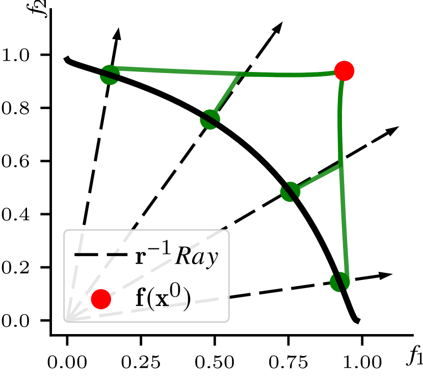
D.3 Further Comparison with Pareto MTL
Our EPO Search algorithm switches from balance mode to descent mode after entering a narrow conical region around the ray. This may appear similar to Pareto MTL (Lin et al. 2019) (described in section 2.3), where in the first phase one finds a solution , where
| (123) |
such that the EPO solution is in , and in the second phase one does pure descent. The construction of is such that is also a cone.
However, their method does not guarantee that the outcome of second phase also lies in . Because while descending, the objective vector may go outside the cone . On the other hand, our method guarantees that the objective vector of the final solution will be inside the cone in (121). Because, if in some iteration the , then a balancing anchor direction is used in the QP to bring it back inside the cone in the subsequent iterations.
Moreover, the angular fineness of their cone , which dictates the accuracy of the final solution, is dependent on how many reference vectors are used, which increases exponentially with the number of objectives . On other hand, the angular fineness of our cone can be set by merely choosing a small value of .
Appendix E Case Study: Personalized Medicine
Drug development is an elaborate, long and expensive process – estimates show the average duration between discovery and market launch to be around 15 years (Ng 2015) and the cost per approved new drug to be roughly $2.6 billion in 2013 dollars (DiMasi et al. 2016) and is continuing to increase (Kiriiri et al. 2020). The entire process consists of multiple stages that can be broadly categorized into: (i) Drug Discovery (ii) Pre-clinical Development (iii) Clinical Trials and (iv) Post-marketing surveillance (Huang et al. 2012, Beninger 2018). The first stage involves finding and validating a biological entity (called “target”, e.g., a gene) and a chemical (which may or may not be a previously used drug) such that their interaction has a therapeutic effect on the considered disease. After such a pair is found, pre-clinical studies are performed to understand the mechanism of drug action, e.g., through experimental studies on response of administering the drug on animals or cells in laboratory conditions. If a drug is found to be safe and efficacious, multiple clinical trials are conducted on increasing number of human subjects. Post-marketing surveillance or pharmacovigilance continues even after the drug is approved and in clinical use, to identify adverse side effects not found in previous stages. Each stage in turn has multiple steps, with several regulatory constraints and complex technical challenges; predictive models are utilized for many tasks at each stage (Vamathevan et al. 2019).
E.1 Task Details
-
•
Drug Target Prediction. Drugs that act on specific disease-causing genes are instrumental for personalized medicine, and are actively studied (Schenone et al. 2013), particularly in early stages of drug discovery. Lab-based genomic techniques to find such drug targets are expensive, time-consuming and have high failure rates; hence, computational methods to predict new targets of drugs are used to prioritize drug-target pairs before subsequent testing (Chen et al. 2020). Large collections of experimental data of known drug targets have been made publicly available that can be used for supervised learning. Using such data, the binary classification task is to predict, for a given drug-gene pair, whether or not the gene can be targeted by the drug.
-
•
Drug Response Prediction. Here we consider a single disease, cancer, that is caused by genetic aberrations leading to uncontrolled cell reproduction. Cells with differing genomic profiles may differ in their response to treatment (Senft et al. 2017). To enable personalized cancer treatment based on individual genomic profiles, the effect of anti-cancer drugs on many cancer cells under laboratory conditions are being actively studied and documented (Yang et al. 2013, Rees et al. 2016). Broadly, in these experiments, cancer cells are subjected to varying concentrations of drugs, whose capacity to inhibit the reproduction of cancer cells is measured. A widely adopted measure of drug efficacy is half maximal inhibitory concentration (IC50) which is the concentration required to inhibit 50% of the cells (Huang et al. 2012). Genomic profiles of cells can be constructed through various measurements and used as feature vectors, containing information relevant to cancer, such as mutations and indicators of gene activity. Experimental data on drug efficacy can be used to build a regression model that predicts, for a given drug and genomic profile, the efficacy of the drug on cells with such a profile. Such models can provide deeper insights into the mechanism of action of the drugs by uncovering the genomic factors that enable therapeutic action of drugs. They can also potentially be used to personalize drug recommendation for cancer patients, whose genomic profiles can be measured in hospitals (Ma et al. 2021). For the genomic profile of a patient, and a given list of drugs (approved for use in the hospital), clinicians typically seek the top ranking drugs that are predicted to be most effective, which in turn can support subsequent decision-making for treatment planning. Thus, in addition to predicting the drug efficacy, it is also important to obtain accurate ranking of drugs based on efficacy for a given genomic profile.
-
•
Drug Side Effect Prediction. Adverse drug events (ADEs) are unintended side effects of drugs that often lead to emergency visits, prolonged hospital stays, and worse patient outcomes (Ventola 2018). Worldwide, they remain a leading cause of morbidity and mortality, posing substantial clinical and economic burden (Watanabe et al. 2018). Clinical trials are limited by the number and characteristics of patients tested as well as the duration of the observation period, and they may not detect all ADEs, especially those with long latency or those that affect only certain patient groups (Coloma et al. 2013). So, pharmacovigilance is routinely conducted to document reports of ADEs of approved drugs. Large databases have been created (Kuhn et al. 2016, Tatonetti et al. 2012) that correct for biases and omissions in the reports due to concomitant medication, patient demographics and medical histories. This enables development of supervised learning models that can be used to predict potential ADEs of a drug, which can be further investigated by pharmacovigilance teams. The problem is that of binary classification, where given a disease-drug pair, the model predicts whether the disease may be a side-effect of a drug.
E.2 Data
Data from multiple publicly available drug-related databases have been collected and preprocessed by Jiang et al. (2021) for integrative analysis. For Drug Target (DT) prediction we use data from STITCH (Szklarczyk et al. 2016), DrugBank (Wishart et al. 2018) and Repurposing Hub (Corsello et al. 2017); for Drug Response (DR) prediction, we use GDSC (Yang et al. 2013) and CCLE (Rees et al. 2016) databases; for Drug Side-effect (DS) prediction, we use SIDER (Kuhn et al. 2016) and OFFSIDES (Tatonetti et al. 2012). A summary of the datasets is given in Table 4; more details can be found in Jiang et al. (2021).
E.3 Additional Details of Model and Training
We used ReLU activation function for all the layers, except the final layers of the predictors; sigmoid activation is used for DT and DS classifiers, and an identity map for DR regressor. The training hyper parameters used are identical for all methods: Adam optimizer with learning rate , mini-batch size of for each training dataset, and K iterations. We did not compare with PMTL, because, as noted in Lin et al. (2019) and observed in our experiment in §5.1, it fails to scale for more than two objectives when the solution space is high-dimensional (in this case, more than 0.73 million).
Appendix F Additional Experimental Results
F.1 Multi-Task Learning in Hydrometeorology
Flooding and other hydrological threats pose critical risks to lives and property, and can impact multiple industries such as agriculture, fishing, forestry, transportation and construction (Adams and Pagano 2016). Billions of dollars are lost in major disasters, including floods, in the US alone (NOAA National Centers for Environmental Information 2022). Timely river flow forecasts play a crucial role in mitigating the adverse effects of such events (Chang et al. 2019). River flow forecasts are also used for water supply management, reservoir operations, and navigation planning. Forecasts are required at strategic sites along rivers where flow levels along with other meteorological variables (e.g., rainfall and temperature) are regularly recorded. A predictive model for all the considered sites can be developed jointly using MTL, where a task is a site-specific prediction.
We use the River Flow dataset (Spyromitros-Xioufis et al. 2016) that has tasks: predicting the flow at sites in the Mississippi River network. Each sample contains, for each site, the most recent and time-lagged flow measurements from hours in the past. Thus, there are features and target variables.
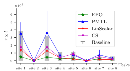
We remove samples with missing values and use samples for training and for testing. We use a fully connected feed-forward neural network (FNN) with layers (layerwise sizes: ) with parameters to fit the data. We randomly choose input priority vectors (with ) and train the FNN using EPO search, PMTL, Linear Scalarization (LinScalar) and Chebychev Scalarization (CS). We use each of the objectives trained separately as baselines. We used Mean Squared Error (MSE) as the loss for each task. For all the methods stochastic gradient descent is used for training with the same hyperparameters: number of epochs, number of mini-batches and learning rate. Since visualization is difficult for 8 dimensions, we compare the methods using the relative loss profile (RLP) on the test data as shown in Figure 15.
We observe that EPO Search outperforms the other methods, indicating that it complies better with the input user priorities; the RLP of EPO search is more uniform (in the sense of definition (33)). The improvement over PMTL is higher in this experiment compared to the e-commerce experiment in F.2 with two tasks. This is expected since the number of reference vectors required by PMTL, to reach a desired ray, grows exponentially with . The problem with the min-max strategy of CS gets highlighted in this experiment showing how combining information from all the task gradients in each iteration is important in an MTL setup. LS does that, therefore performs better than CS in this experiment. However, it does not comply with the priority specification, resulting in a non-uniform RLP in Figure 15. Interestingly, except PMTL, all other MOO based MTL methods improve over the baseline which shows the advantage of MTL for correlated tasks over learning each task independently: predicting river flow at one site helps improving the prediction at other sites as all the sites are from the same river.
F.2 Multi-Task Learning in E-Commerce
Fashion and lifestyle items, such as bags, footwear and apparel, constitute a large portion of e-commerce sales (Elahi and Qi 2020, Deldjoo et al. 2022). Visual appearance of these items plays an influential role in purchase decisions. Search and recommendation engines in e-commerce websites, that are traditionally based on text-based keywords and descriptions, are increasingly using systems that can utilize images directly (Cheng et al. 2021). An important element in such systems is a classifier that can classify the input image into various categories, in order to restrict subsequent search and recommendation within the category. In many cases the image may have multiple items, for instance in bundled sales, from the same or different categories. When multiple items are present in the input image MTL can be effectively used, by considering each task as a classification problem for an item in the image (Lin et al. 2020).
We use three benchmark classification datasets: (1) MultiMNIST, (2) MultiFashion, and (3) Multi-Fashion+MNIST. In the MultiMNIST dataset (Sabour et al. 2017), two images of different digits are randomly picked from the original MNIST dataset (LeCun et al. 1998), and combined to form a new image, where one is in the top-left and the other is in the bottom-right. There is zero padding in the top-right and bottom-left. The MultiFashion dataset is generated in a similar manner from the FashionMNIST dataset (Xiao et al. 2017). In Multi-Fashion+MNIST dataset, one image is from MNIST (top-left) and the other image is from FashionMNIST (bottom-right). In each dataset, there are samples in the training set and samples in the test set.
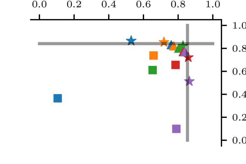
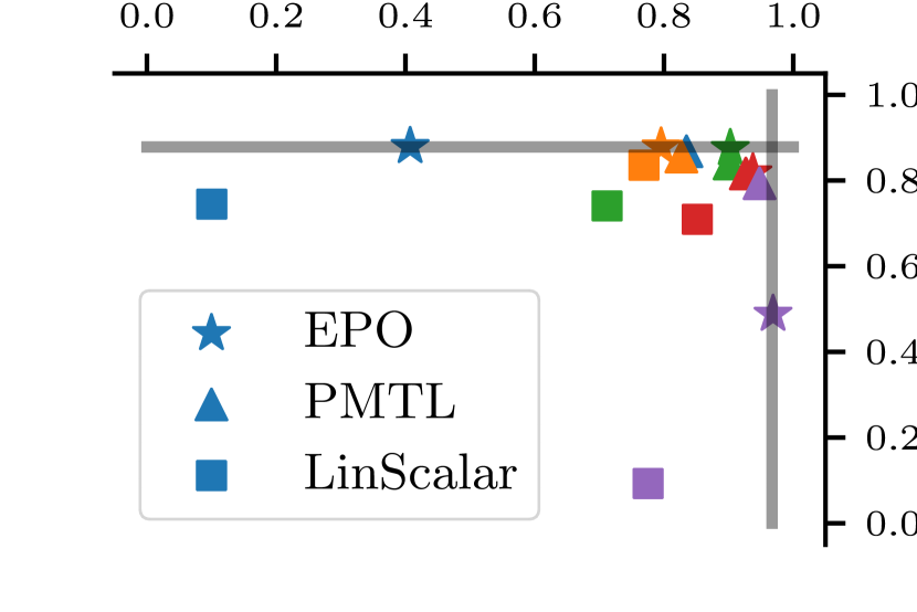
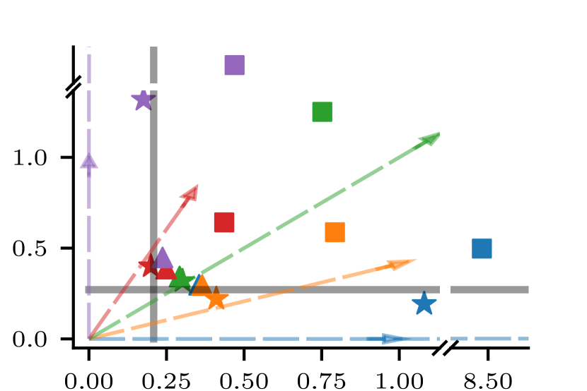
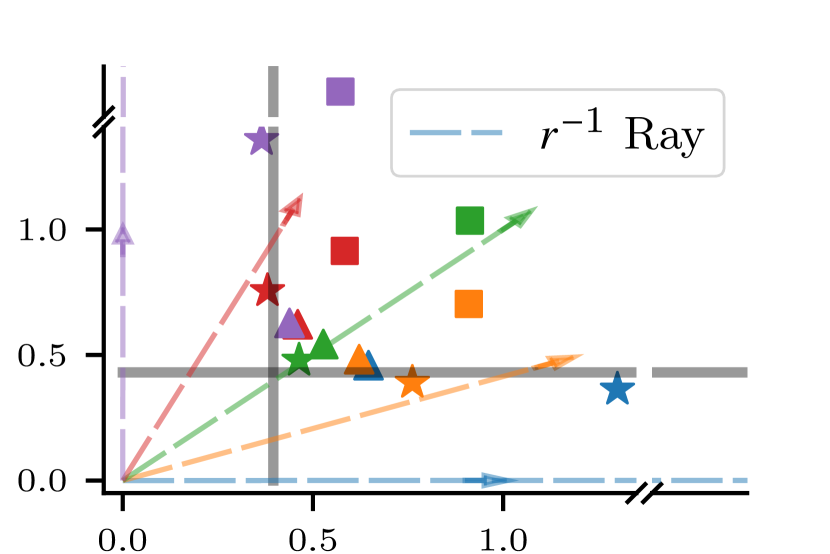
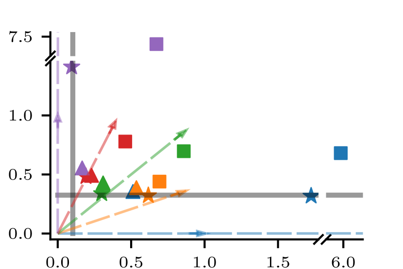
For each dataset, there are two tasks: 1) classifying the top-left image, and 2) classifying the bottom-right image. Cross entropy losses are used for training. We use the same network (LeNet (LeCun et al. 1998) with 31,910 trainable free parameters) used in Lin et al. (2019) as the MTL neural network. The baseline for comparison is training the network for individual tasks. In addition we compare with the results from linear scalarization (LinScalar) and Chebyshev Scalarization.
For all the methods stochastic gradient descent is used for training with the same hyperparameters: number of epochs, number of mini-batches and learning rate. We test the performance of all methods for the same 5 vectors, shown as rays in the bottom row of Figure 16. Ideal solutions should lie on these rays. Thus, each method has exactly 5 points corresponding to the test set losses in the bottom row and the top row shows the test set accuracies of the corresponding 5 DNN solutions.
The results in Figure 16. show that the per-task accuracy of EPO search is higher than that of PMTL in every single run (top). The test set losses (bottom) show that the solutions from EPO search are closer to the corresponding vectors, compared to the solutions from PMTL. For the reasons discussed in previous experiments, our method outperforms CS. To avoid clutter in the Figures 16, the results of CS are not shown. We observe that the performance of LinScalar is worse than all the other methods.
Apart from the domains, the 3 applications we consider also differ in terms of predictive models developed for the tasks, data usage, and subsequent use of the model. In application 1 (personalized medicine), the tasks considered are different and the corresponding predictive models are typically developed independently with data sources that are partly shared and partly task-specific. In contrast, in application 3 (e-commerce), the tasks are identical, use the same data sources for model building and, most often, are used together in subsequent applications. Application 2 (hydrometeorology) is similar to the third one in terms of the prediction task and data used for model building. However, models for each task may or may not be used together subsequently.
Appendix G Preference Elicitation
PE methods may be classified based on how the utility function is modeled.
Deterministic PE. Here the utility function is modelled deterministically, i.e., as a parametric function of the objective values. E.g., Zionts and Wallenius (1976) used linear scalarization of the objectives as the utility function, which cannot model all Pareto optimal solutions as DM’s preferred solution for non-convex MOO problems. Since LS cannot model all PO solutions for non-convex MOO problems, many interactive methods, such as Steuer (1989), Steuer et al. (1993), Dell and Karwan (1990), Ozbey and Karwan (2014), Reeves and MacLeod (1999), were developed that use Chebyshev scalarization as utility function due to its ability to model all the Pareto optimal solutions, even for non-convex objectives. Chebyshev scalarization can be considered as a proxy utility function to reach the best preferred alternative for the DM. These Weight Space Reduction Methods reduce the parameter space of the utility, after every interaction, to be consistent with the DM’s responses. However, interactive MCDM with Chebyshev utility is inefficient, because the reduced weight space consists of several disconnected components, which grows exponentially with the number of interactions with the DM. Therefore, selecting a weight from the fragmented weight space to probe for the next alternative becomes computationally expensive for large and complex problems (Miettinen 1998).
Another deterministic PE approach is Preference Robust Optimization (PRO), where the set of all possible utility functions are restricted to only those that are consistent with the previous pair-wise comparisons, and the worst utility in this restricted set is optimized to find the next alternative. E.g., Vayanos et al. (2020) model the utility as a linear function and Haskell et al. (2018) model it as a quasi-concave function, using several support (“hockey stick”) functions, where the number of parameters of the utility function grows linearly with the number of interactions. PRO methods assume the MOO to be convex and the utility to be quasi-convex in the most general case. They cannot model non-convex PE problems, where either the MOO problem or the utility function could be non-convex.
Probabilistic PE. Here, the utility function is modelled using probabilistic methods. There are parametric models of utility for probabilistic PE, e.g., Armbruster and Delage (2015) which does not model non-convex utility functions. In contrast, non-parametric methods, such as Gaussian processes can model any class of functions – see §H and 2.2.2.
Appendix H Bayesian optimization with Gaussian Process
Bayesian optimization (BO) is a sequential model-based approach for solving black-box function optimization problems (see, e.g. Shahriari et al. (2016)). The key idea is to learn a surrogate probabilistic model that captures our beliefs about the unknown function . The functional form of is unknown but it is assumed that the function can be evaluated at any given point x. The model is learnt from data, = , that consists of sequential evaluations of for different values of x.333Note, in our setup of PE, we do not have direct evaluation of the utility at a point . Instead the data is in the form of pairwise comparisons such that .
Generating this data sequence requires making the decision of which x to evaluate next, at each step. This decision is made through an acquisition function . These functions are designed to have optima at points with high uncertainty in the surrogate model (thus facilitating exploration) and/or at points with high predictive values in the surrogate model (thus facilitating exploitation). Acquisition functions have known functional forms and are usually easier to optimize than the original objective function. The surrogate model is updated sequentially with each observed data point. Over multiple steps, the landscape of the black-box function is learnt by the surrogate model and can be exploited by the acquisition function to yield values of x that are, on average, closer to the optimal .
Many different choices of surrogate models and acquisition functions have been explored. A Gaussian process (GP) may be used to model priors over functions. GPs can be viewed as an infinite-dimensional extension to a multivariate Gaussian distribution (Rasmussen and Williams 2004), and can approximate general non-linear functions. A is specified by a mean function and a covariance function , e.g., Gaussian or Matérn kernel. This models the uncertainty in the unknown objective function value at a particular solution as a Gaussian distribution, . The joint probability of the function values at more than one solution, e.g., , is modelled as multivariate Gaussian, , where is the gram matrix of kernel evaluated at .
A common choice for the acquisition function is Expected Improvement (EI) (Jones 2001), that has a closed form for GP, does not require its own tuning parameter and has been shown to perform well (Snoek et al. 2012). EI is the expectation that will improve over which is the best observation from steps of BO so far, i.e. , and , where the expectation is under the posterior distribution given evaluations of at . The next value is chosen by . For a GP with predictive variance and predictive mean :
| (124) |
where, , and and denote the CDF and PDF of the standard normal distribution respectively.
Appendix I Optimization in Neural Networks
A neural network is a parametric function , where is the input dimension and is the target dimension, created by composition of multiple constituent functions represented by layers in the network. For example a three layered network can be written as
| (125) |
where is the set of parameters for the layer , and are the input and output dimensions of the layer (here , and ). A layer performs an affine transformation followed by an elementwise nonlinear transformation, e.g., sigmoid or ReLU. The function parameters (aka network weights) are learnt by optimizing the training objective which is determined by the learning task and targets given by a training dataset :
| (126) |
where is a differentiable loss function measuring the deviation of the output from the expected value . Common loss functions include the mean-squared error loss for regression tasks and cross-entropy loss for classification tasks. Note, here ’s are not the variables of optimization, they are input data features and ’s are the targets. It is customary in the neural network literature to denote the model parameters, which are the optimization variables, as . A neural network with three or more layers is generally considered deep. Training such a model requires learning large number of parameters, which makes it prohibitively expensive to use second-order methods. First order optimization techniques, based on gradient descent, are most widely used. More details can be found in books on deep learning, e.g., by Goodfellow et al. (2016).
I.1 Deep Neural Networks for Multi-task Learning
In MTL, there are more than one training objectives each stemming from a task. The MTL datasets may have multiple targets, for different tasks, e.g., has targets for different tasks and a common input for all of them, like in our experiments in §F. Another example of a MTL dataset is , where there is a common input for all the tasks, task specific inputs , for each task, and the corresponding targets , , like in our experiment in §5.5.
MTL models are designed according to the format of data. For example, the model in Figure 2 can be considered as two parametric functions designed for the first type of MTL dataset:
| (127) |
where is the network parameter for embedding the common input, and ’s are for the task specific layers. The simultaneous optimization problems for training this model is given by
| (128) |
where ’s are task-specific loss functions.