Convergence of a finite difference scheme for the Kuramoto–Sivashinsky equation defined on an expanding circle

Abstract

This paper presents a finite difference method combined with the Crank–Nicolson scheme of the Kuramoto–Sivashinsky equation defined on an expanding circle (KUY ), and the existence, uniqueness, and second-order error estimate of the scheme. The equation can be obtained as a perturbation equation from the circle solution to an interfacial equation and can provide guidelines for understanding the wavenumber selection of solutions to the interfacial equation. Our proposed numerical scheme can help with such a mathematical analysis.

1 Introduction

A mathematical analysis of the behavior of a gaseous combustion flame front has long been under study, starting with the pioneering research by Sivashinsky S . In recent years, the behavior of the flame front during the smoldering combustion on a thin solid (e.g. a sheet of paper) has been vigorously studied both experimentally (GKKY ; KSTK ; OBK ; ZOM ; ZM1 ; ZM2 ; ZRRG ) and mathematically (FMP ; GKUY ; GKY ; IIMO1 ; IIMO2 ; IM1 ; IM2 ; KKUYB ; KS ) aspects. The Kuramoto–Sivashinsky (KS) equation (KT ; S ), which is a well-known mathematical model of gaseous combustion, has been applied to research on smoldering combustion (GKKY ; GKUY ; GKY ; KKUYB ).

The purpose of the present paper is to numerically solve the following time evolution equation (KUY ), which represents the interface of a combustion front spreading over time as a closed curve:

$$\dfrac{\partial u}{\partial t}+\dfrac{\delta}{R^{4}}\dfrac{\partial^{4}u}{\partial\sigma^{4}}+\dfrac{1}{R^{2}}\left(\alpha-1+\dfrac{\delta}{R^{2}}\right)\dfrac{\partial^{2}u}{\partial\sigma^{2}}+\dfrac{\alpha-1}{R^{2}}u-\dfrac{v_{c}}{2R^{2}}\left(\dfrac{\partial u}{\partial\sigma}\right)^{2}=0,\\$$ (1)

where the solution $u:[0,2\pi]\times(0,T);(\sigma,t)\mapsto\mathbb{R}$ denotes a height function from an expanding circle solution of (2) (that is, the solution of (6) defined below) with radius $R=R(t)$ at time $t$, $\delta$ is a positive parameter, $\alpha>0$ is a scaled Lewis number, and $v_{c}$ corresponds to a constant velocity for a uniformly traveling wave described through (3) below.

(1) is a perturbed equation of an expanding circle solution of the following time evolution equation:

$$\dfrac{\partial\bm{X}}{\partial t}=V\bm{N}+W\bm{T},\quad V=v_{c}+(\alpha-1)\kappa+\delta\dfrac{\partial^{2}\kappa}{\partial s^{2}},$$ (2)

which is a flow of a family of smooth Jordan curves $\{\mathrm{\Gamma}(t)\}_{0\leq t\leq T}$ in the plane $\mathbb{R}^{2}$. The solution curve $\mathrm{\Gamma}(t)$ is parameterized by a smooth mapping $\bm{X}=\bm{X}(\sigma,t):\,[0,2\pi]\times[0,T]\to\mathbb{R}^{2}$ such as $\mathrm{\Gamma}(t)=\{\bm{X}(\sigma,t);\,\sigma\in[0,2\pi]\}$ (in which the positive direction of $\Gamma(t)$ is counterclockwise). In the second equation in (2), $\kappa$ denotes the curvature of $\mathrm{\Gamma}(t)$, and $\partial^{2}\kappa/\partial s^{2}$ is the second derivative of $\kappa$ with respect to the arc-length parameter $s=\int_{0}^{\sigma}g(\sigma,t)d\sigma$, where $g=|\bm{X}_{\sigma}|$ is the local length, $\bm{X}_{\sigma}=\partial\bm{X}/\partial\sigma$, and $\partial\kappa/\partial s=g^{-1}\partial\kappa/\partial\sigma$. The velocity of the curve is $\partial\bm{X}/\partial t$, which can be decomposed in the outward normal direction $\bm{N}=-\bm{T}^{\bot}$ and the tangential direction $\bm{T}=\bm{X}_{\sigma}/|\bm{X}_{\sigma}|$. It is well known that the shape of the curves $\mathrm{\Gamma}(t)$ is determined by the normal velocity $V$ only, and that the tangential velocity $W$ does not affect its shape (see Epstein and Gage EG ). The details of the derivation from (2) to (1) are provided in subsection 2.1. At a certain scale, (2) is equivalent to the KS equation:

$$\dfrac{\partial f}{\partial t}+\delta\dfrac{\partial^{4}f}{\partial x^{4}}+(\alpha-1)\dfrac{\partial^{2}f}{\partial x^{2}}+\dfrac{v_{c}}{2}\left(\dfrac{\partial f}{\partial x}\right)^{2}=0,$$ (3)

where $f:[0,L]\times\mathbb{R}_{+};(x,t)\mapsto\mathbb{R}$ represents a graph of perturbation for a unidirectional uniformly traveling wave solution (see FS and GKY for details). From the point of view of the gaseous combustion theory, $\delta$ is considered to be $4$ when $\alpha$ is close to $1$. We remark that by changing the variables such that $f(x,t)=-u(\sigma,t)$, $x=R\sigma$ with a constant $R$, and taking the limit $R\to\infty$, (3) can be formally obtained from (1). In this sense, (1) corresponds to KS equation (3).

In this paper, to analyze (1), we rewrite (1) using $v=\partial u/\partial\sigma$ as

$$\dfrac{\partial v}{\partial t}+\dfrac{\delta}{R^{4}}\dfrac{\partial^{4}v}{\partial\sigma^{4}}+\dfrac{1}{R^{2}}\left(\alpha-1+\dfrac{\delta}{R^{2}}\right)\dfrac{\partial^{2}v}{\partial\sigma^{2}}+\dfrac{\alpha-1}{R^{2}}v-\dfrac{v_{c}}{R^{2}}v\dfrac{\partial v}{\partial\sigma}=0,$$ (4)

and we impose (4) under the zero average condition $\int_{0}^{2\pi}v(\sigma,t)d\sigma=0$ and the periodic boundary condition $v(\sigma,t)=v(\sigma+2\pi,t)$.

The KS equation (3), which was originally derived as a model of the flame front propagation by Sivashinsky S , and independently as the phase turbulence in the reaction-diffusion system by Kuramoto and Tsuzuki KT , has been extensively studied for nearly 40 years, both based on the theory of combustion phenomena and in applied mathematics. From a mathematics perspective, it is well known that (3) has a rich solution structure including the so-called spatio-temporal chaos (MS ; SM ), and therefore, many researchers of dynamical systems theory, partial differential equation theory, and numerical analysis have been attracted. In particular, the existence and uniqueness of the solutions (AM ; NS ; T ), the existence and estimates of the Hausdorff and fractal dimensions estimates for an inertial manifold (NST ; R ), the bifurcation structures through a Fourier mode interaction (AGH1 ; AGH2 ; PK ) and numerical studies on for the dynamical behavior (HN ; PS ) are still actively being researched.

In the context of a numerical analysis, in A1 , Akrivis applied a finite difference scheme to (3) under a periodic boundary condition. The method used to prove our result upon convergence to (4) is based on the idea of A1 , and is extended to our scheme for (1). Akrivis also reported in A2 a consistent numerical approach to solving (3) by using a finite element Galerkin method with an extrapolated Crank–Nicolson scheme. In both cases, a rigorous error analysis was carried out in order to derive the refined error bound. In addition, numerous other methods have been proposed to find the numerical solutions to (3) (see BC and the references therein).

We emphasize that (1) and (4) are moving boundary problems (by contrast, (3) is formulated in a fixed region), and it is therefore difficult to apply standard dynamical systems theory and analyze the detailed solution structure through a bifurcation analysis. These facts motivated us to study the behavior of the solution from a numerical aspect. The results given in Section 4.4 of the present paper, guarantee the guidelines for the wavenumber and parameter selection suggested in KUY .

The present paper is organized as follows. In section 2.1, we show that (1) is equivalent to an interfacial equation, which was introduced as a combustion model by Frankel and Sivashinsky FS . Our main results are listed in the following section. In sections 2.2 and 2.3, convergence of the solutions to the Crank-Nicolson scheme and Newton’s method are presented, respectively. Our main result of the convergence is described in section 2.4, which is summarized as

$$\max_{0\leq n\leq N}\|\bm{u}^{n}-\bm{U}^{n}\|_{h}\leq c(k^{2}+h^{2}),$$

where $\|\cdot\|_{h}$ denotes the discrete $\mathscr{L}^{2}$-norm with the space increment $h$, $\bm{u}^{n}$ is a vectorized solution to (1) at the $n$-th time step $t^{n}=nk$ with the time increment $k$, and $\bm{U}^{n}$ is an approximation solution at the $n$-th step. In section 3, we give the proofs of the main theorems presented in section 2, that is, show the existence, convergence and uniqueness to our scheme. In section 4.1, the algorithm used by our scheme is given. In section 4.2, several numerical experiments of the solution curves are shown. In the remaining part of section 4, we focus on a theoretical linearized stability analysis, particularly the bifurcation theory of the relation between the wavenumber and parameters for moving solution curves and its numerical analysis. In the final section 5, we provide some concluding remarks and areas of future study.

2 Main results

2.1 Derivation (1) from an interfacial equation

For convenience, in this subsection, the derivation of (1) from (2) for a certain space and time scale is given according to KUY .

(2) has a circle solution

$$\bm{X}(\sigma,t) =\bm{X}_{R}=R(t)\bm{y}(\sigma),\quad\bm{y}=\begin{pmatrix}\cos{\sigma}\\ \sin{\sigma}\end{pmatrix},$$ (5)

$$\dfrac{dR}{dt} =v_{c}+\dfrac{\alpha-1}{R}.$$ (6)

The solution to (6) is

$$\dfrac{1}{V_{0}}\left\{R(t)-R(0)-\dfrac{\alpha-1}{v_{c}}\log{\dfrac{v_{c}R(t)+\alpha-1}{v_{c}R(0)+\alpha-1}}\right\}=t,$$ (7)

which will be used in our numerical scheme (see Section 4). The following property is easily shown.

Proposition 1 (Proposition 1 in KUY )

Let $\alpha-1>0$. Then, for any $R(0)>0$, the solution $R(t)$ strict monotonically increases, and $R(t)\to+\infty$ holds as $t\to+\infty$.

We now consider a perturbation, e.g., $u(\sigma,t)$, of the circle solution (5) such that $\bm{X}-\bm{X}_{R}=u(\sigma,t)\bm{y}$. By taking the inner product of (2) and $\bm{N}$, and denoting $\partial^{j}\bm{X}/\partial\sigma^{j}=F_{j}\bm{y}+G_{j}{\bm{y}^{\bot}}$ ($(a,b)^{\bot}=(-b,a)$), (2) yields

$$\dot{R}+\dot{h}=\dfrac{v_{c}g}{G_{1}}+\dfrac{1}{g^{2}}\left(\dfrac{F_{1}G_{2}}{G_{1}}-F_{2}\right)\left\{(\alpha-1)+\dfrac{3\delta}{g^{3}}\left(\dfrac{5g_{\sigma}^{2}}{g}-g_{\sigma\sigma}\right)\right\}$$ (8)

$$+\dfrac{\delta}{g^{4}}\left\{\dfrac{F_{1}G_{4}}{G_{1}}-F_{4}-\dfrac{7g_{\sigma}}{g}\left(\dfrac{F_{1}G_{3}}{G_{1}}-F_{3}\right)+\dfrac{F_{2}G_{3}-F_{3}G_{2}}{G_{1}}\right\}.$$

We set $\varepsilon=|\alpha-1|>0$ as a small parameter and rescale (8) from $u$ to $f$ using $\varepsilon$ such that $u(\sigma,t)=\varepsilon f(\sigma,\tau)$, $\tau=\varepsilon^{2}t$, and $r=\varepsilon^{1/2}R$. Thus, (8) can be rewritten as

$$\Bigg{(}\dfrac{\partial f}{\partial\tau}+\dfrac{\delta}{r^{4}}\dfrac{\partial f^{4}}{\partial\sigma^{4}}+\dfrac{1}{r^{2}}\left(\textrm{sgn}(\alpha-1)+\dfrac{\delta}{r^{2}}\right)\dfrac{\partial f}{\partial\sigma}$$

$$\qquad+\dfrac{\textrm{sgn}(\alpha-1)}{r^{2}}f-\dfrac{v_{c}}{2r^{2}}\left(\dfrac{\partial f}{\partial\sigma}\right)^{2}\Bigg{)}\varepsilon^{3}+o(\varepsilon^{3})=0.$$

Because $\alpha-1=\textrm{sgn}(\alpha-1)\varepsilon$, omitting the term $o(\varepsilon^{3})$ and replacing $f$ with $u=u(\sigma,t)\in\mathbb{R}$, one can extract (1) at the original scale. Throughout this paper, we assume $u(\sigma,t)\in C^{\infty}$ and $2\pi$-periodic function on $\sigma$, i.e., $u(\sigma,t)=u(\sigma+2\pi,t)$. In addition, we set $u(\cdot,0)=u_{0}(\sigma)$ and $R(0)=R_{0}>0$ as the initial conditions.

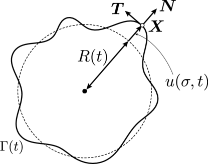
Figure 1: Schematic image of the circle solution to (2) and a perturbation $u(\sigma,t)$.

2.2 Convergence of solutions to Crank–Nicolson scheme

We now state our main results, which will be proved in Section 3. Let $J\in\mathbb{N}$, $N\in\mathbb{N}$, $T>0$, $L=2\pi$, $h=L/J$, $\sigma_{i}=ih$, $i\in\mathbb{Z}$, $k=T/N$, $t^{n}=nk$ $(n=0,1,\dots,N)$ and

$$\mathbb{R}^{J}_{\mathrm{per}}:=\{\bm{V}=(V_{i})_{i\in\mathbb{Z}};\,V_{i}\in\mathbb{R}\quad\textrm{and}\quad V_{i+J}=V_{i},\quad i\in\mathbb{Z}\}.$$

For $\bm{V}\in\mathbb{R}^{J}_{\mathrm{per}}$, we describe

$$\Delta_{h}V_{i} =\dfrac{1}{h^{2}}(V_{i-1}+2V_{i}+V_{i+1}),$$

$$\Delta_{h}^{2}V_{i} =\dfrac{1}{h^{2}}(\Delta_{h}V_{i-1}-2\Delta_{h}V_{i}+\Delta_{h}V_{i+1})$$

and for $\bm{V}^{0},\dots,\bm{V}^{N}\in\mathbb{R}^{J}_{\mathrm{per}}$, we set

$$\partial\bm{V}^{n}=\dfrac{1}{k}(\bm{V}^{n+1}-\bm{V}^{n}),\quad\bm{V}^{n+\frac{1}{2}}=\dfrac{1}{2}(\bm{V}^{n}+\bm{V}^{n+1}).$$

We discretize the equation (4) using the Crank–Nicolson type finite difference scheme. More precisely, we approximate $\bm{v}^{n}\in\mathbb{R}^{J}_{\mathrm{per}}$ ($v^{n}_{i}=v(\sigma_{i},t^{n})$) using $\bm{V}^{n}\in\mathbb{R}^{J}_{\mathrm{per}}$, where $\bm{V}^{0}=\bm{v}^{0}$, and for $n=0,1,\dots,N-1$

$$\begin{multlined}\partial\bm{V}^{n}+\mathcal{L}_{h}^{n+\frac{1}{2}}\bm{V}^{n+\frac{1}{2}}=\dfrac{v_{c}}{6hR_{n+\frac{1}{2}}^{2}}\bm{\varphi}(\bm{V}^{n+\frac{1}{2}},\bm{V}^{n+\frac{1}{2}}),\quad i=1,\dots,J.\end{multlined}\partial\bm{V}^{n}+\mathcal{L}_{h}^{n+\frac{1}{2}}\bm{V}^{n+\frac{1}{2}}=\dfrac{v_{c}}{6hR_{n+\frac{1}{2}}^{2}}\bm{\varphi}(\bm{V}^{n+\frac{1}{2}},\bm{V}^{n+\frac{1}{2}}),\quad i=1,\dots,J.$$ (9)

Hereafter, we set $R_{n}=R(t^{n})$,

$$\mathcal{L}_{h}^{n}:\,\mathbb{R}^{J}_{\mathrm{per}}\to\mathbb{R}^{J}_{\mathrm{per}};$$

$$\quad\left(\mathcal{L}_{h}^{n}\bm{V}\right)_{i}:=\dfrac{\delta}{R_{n}^{4}}\Delta_{h}^{2}V_{i}+\dfrac{1}{R_{n}^{2}}\left(\alpha-1+\dfrac{\delta}{R_{n}^{2}}\right)\Delta_{h}V_{i}+\dfrac{\alpha-1}{R_{n}^{2}}V_{i},$$

and

$$\bm{\varphi}:\,\mathbb{R}^{J}_{\mathrm{per}}\times\mathbb{R}^{J}_{\mathrm{per}}\to\mathbb{R}^{J}_{\mathrm{per}};$$

$$\quad\left(\bm{\varphi}(\bm{V},\bm{W})\right)_{i}=(V_{i-1}+V_{i}+V_{i+1})(W_{i+1}-W_{i-1}).$$

Remark that $R(t)$ is a given function.

The discrete $\mathscr{L}^{2}$-norm $\|\cdot\|_{h}$ is introduced in $\mathbb{R}^{J}_{\mathrm{per}}$ the discrete $\mathscr{L}^{2}$-norm $\|\cdot\|_{h}$ using

$$\|\bm{V}\|_{h}:=\left(h\sum_{i=1}^{J}(V_{i})^{2}\right)^{\frac{1}{2}},\quad\bm{V}\in\mathbb{R}_{\mathrm{per}}^{J},$$

which is induced through the $\mathscr{L}^{2}$-inner product $(\cdot,\cdot)_{h}$ in $\mathbb{R}_{\mathrm{per}}^{J}$ such that

$$(\bm{V},\bm{W})_{h}:=h\sum_{i=1}^{J}V_{i}W_{i},\quad\bm{V},\bm{W}\in\mathbb{R}_{\mathrm{per}}^{J}.$$

We can then obtain the result regarding the existence of the numerical solution to (9):

Proposition 2

Let $R(0)>\sqrt{\delta/(\alpha-1)}$ and

$$k<\dfrac{8\delta}{\left(\alpha-1-\dfrac{\delta}{R(T)^{2}}\right)^{2}}.$$ (10)

Then, an approximate solution to (9) exists.

As one of the main results in this paper, the following insists that the second-order error estimate to the Crank–Nicolson scheme holds:

Theorem 2.1

Let $v$ be sufficiently smooth, and let $M$ be a positive constant such that $\displaystyle\sup_{0\leq t\leq T}\left\|\dfrac{\partial v}{\partial\sigma}\right\|_{\infty}\leq M$. Suppose that $\bm{V}_{\mathrm{CN}}^{1},\dots,\bm{V}_{\mathrm{CN}}^{N}\in\mathbb{R}_{\mathrm{per}}^{J}$ are solutions to (9) with the initial data $\bm{V}_{\mathrm{CN}}^{0}=\bm{v}^{0}$. Then, for a sufficiently small $k$, there exists a constant $c=c(\delta,\alpha,R_{0},M)$ independent of $k$ and $h$ such that

$$\max_{0\leq n\leq N}\|\bm{v}^{n}-\bm{V}_{\mathrm{CN}}^{n}\|_{h}\leq c(k^{2}+h^{2}).$$ (11)

Hereafter, $c$ and $C$ denote general constants that are independent of $k$ and $h$, and do not need to be the same in any two places unless subscripts are applied. Furthermore, for a sufficiently small $kh^{-\frac{1}{5}}$, the Crank–Nicolson approximations are uniquely defined by (9):

Proposition 3

Under the same assumption as in Theorem 2.1, for a sufficiently small $kh^{-\frac{1}{5}}$, the solution to the Crank–Nicolson scheme is unique.

2.3 Convergence of solutions to Newton’s method

To compute the Crank–Nicolson approximations $\bm{V}_{\mathrm{CN}}^{1},\dots,\bm{V}_{\mathrm{CN}}^{N}$, it is necessary to solve a $J\times J$ nonlinear system at each time step. In this section, we discuss the approximate solution to (9) using the following Newton’s method.

For $n\geq 0$, the linearized system using Newton’s method is

$$\partial\bm{W}^{n}+\mathcal{L}_{h}^{n+\frac{1}{2}}\bm{W}^{n+\frac{1}{2}} =\dfrac{v_{c}}{24hR_{n+\frac{1}{2}}^{2}}\bigg{(}\bm{\psi}(\bm{W}^{n}+\hat{\bm{W}}^{n+1},\bm{W}^{n+1}-\hat{\bm{W}}^{n+1})$$ (12)

$$+\bm{\varphi}(\bm{W}^{n}+\hat{\bm{W}}^{n+1},\bm{W}^{n}+\hat{\bm{W}}^{n+1})\bigg{)}.$$

Here, $\hat{\bm{W}}^{0}:=\bm{v}^{0}$, $\hat{\bm{W}}^{n+1}:=2\bm{W}^{n}-\bm{W}^{n-1}$ $(n\geq 1)$ and $\hat{\bm{W}}^{1}$ is given by

$$\begin{multlined}\partial\hat{\bm{W}}^{0}+\mathcal{L}_{h}^{\frac{1}{2}}\hat{\bm{W}}^{\frac{1}{2}}-\dfrac{v_{c}}{6hR_{\frac{1}{2}}^{2}}\bm{\varphi}(\bm{v}^{0},\bm{v}^{0})=0.\end{multlined}\partial\hat{\bm{W}}^{0}+\mathcal{L}_{h}^{\frac{1}{2}}\hat{\bm{W}}^{\frac{1}{2}}-\dfrac{v_{c}}{6hR_{\frac{1}{2}}^{2}}\bm{\varphi}(\bm{v}^{0},\bm{v}^{0})=0.$$ (13)

Note that the symbol “ $\hat{}$ ” indicates the initial value when applying Newton’s method. Although it is still complicated to compute $\bm{W}^{n+1}$, and because (12) is a $J\times J$ linear system whose matrix depends explicitly on $\bm{W}^{n}$ and $\bm{W}^{n-1}$, to simplify the problem, we will approximate the solution vectors $\bm{W}^{n}$ through the following process.

For every time steps, we set $j_{n}\in\mathbb{N}$ $(n=1,2,\dots,N)$ as the maximum number of iterations of Newton’s method. We define the sequences of the approximation vectors as $\bm{W}^{n,j}\in\mathbb{R}_{\mathrm{per}}^{J}$ $(j=0,1,\dots,j_{n})$ and $\bm{V}_{\mathrm{Newton}}^{n}:=\bm{W}^{n,j_{n}}$, which corresponds to the approximation solution vector of $\bm{V}_{\mathrm{CN}}^{n}$. More precisely, letting $\bm{V}_{\mathrm{Newton}}^{0}:=\bm{V}_{\mathrm{CN}}^{0}=\bm{v}^{0}$, $\hat{\bm{W}}^{1}=\hat{\bm{V}}^{1}:=\bm{V}_{\mathrm{Newton}}^{1}$, $\bm{W}^{n+1,0}:=\hat{\bm{V}}_{\mathrm{Newton}}^{n+1}$ and replacing $\bm{W}^{n+1}$ on the left hand side and $\bm{\psi}$ of (12) with $\bm{W}^{n+1,j+1}$ and $\bm{W}^{n+1,j}$, respectively, we solve the following:

$$\dfrac{1}{k}(\bm{W}^{n+1,j+1}-\bm{V}_{\mathrm{Newton}}^{n})+\mathcal{L}_{h}^{n+\frac{1}{2}}(\bm{W}^{n+1,j+1}+\bm{V}_{\mathrm{Newton}}^{n})$$ (14)

$$=\dfrac{v_{c}}{24hR_{n+\frac{1}{2}}^{2}}\big{(}\bm{\psi}(\bm{V}_{\mathrm{Newton}}^{n}+\hat{\bm{V}}_{\mathrm{Newton}}^{n+1},\bm{W}^{n+1,j}-\hat{\bm{V}}_{\mathrm{Newton}}^{n+1})$$

$$+\bm{\varphi}(\bm{V}_{\mathrm{Newton}}^{n}+\hat{\bm{V}}_{\mathrm{Newton}}^{n+1},\bm{V}_{\mathrm{Newton}}^{n}+\hat{\bm{V}}_{\mathrm{Newton}}^{n+1})\big{)}.$$

where $j=0,\dots,j_{n+1}-1$. Then, for $R(0)>\sqrt{\delta/(\alpha-1)}$ and (10), the coefficient matrix of the linear systems (13) and (14) is positive definite, as shown in Proposition 2.

The following result guarantees that the estimate of the form (11) holds, that is, the second-order error estimates for the scheme (14) are given.

Theorem 2.2

Suppose that $\bm{V}_{\mathrm{Newton}}^{1},\dots,\bm{V}_{\mathrm{Newton}}^{N}\in\mathbb{R}_{\mathrm{per}}^{J}$ are solutions to (13) and (14) with the initial data $\bm{V}_{\mathrm{Newton}}^{0}=\bm{v}^{0}$. Under the same assumption as in Theorem 2.1, for a sufficiently small $k$ and $h$ satisfying $k=o(h^{\frac{1}{4}})$, we have

$$\max_{0\leq n\leq N}\|\bm{v}^{n}-\bm{V}_{\mathrm{Newton}}^{n}\|_{h}\leq c(k^{2}+h^{2}).$$ (15)

2.4 Main results of convergence

Let $\bm{V}^{n}$ be $\bm{V}_{\mathrm{CN}}^{n}$ or $\bm{V}_{\mathrm{Newton}}^{n}$. The numerical solution to the integral form (1), e.g., $U_{i}^{n}$, can be easily calculated from $V_{i}^{n}$ as follows.

We describe $u_{i}^{n}=u(\sigma_{i},t^{n})$ as

$$u_{i}^{n}=\dfrac{1}{2\pi}\int_{0}^{2\pi}u(\sigma,t^{n})d\sigma-\dfrac{1}{2\pi}\int_{0}^{2\pi}\left(\int_{0}^{\sigma}v(\xi,t^{n})d\xi\right)d\sigma+\int_{0}^{\sigma_{i}}v(\xi,t^{n})d\xi.$$ (16)

The mean value $I(t):=\frac{1}{2\pi}\int_{0}^{2\pi}u(\sigma,t)d\sigma$ satisfies

$$\dot{I}(t)=-\dfrac{\alpha-1}{R(t)^{2}}I(t)+\dfrac{v_{c}}{4\pi R(t)^{2}}\int_{0}^{2\pi}v(\sigma,t)^{2}d\sigma,$$ (17)

and therefore

$$I(t)=\dfrac{\dot{R}(t)}{\dot{R}(0)}\left[I(0)+\dfrac{v_{c}}{4\pi\dot{R}(0)}\int_{0}^{t}\left(\dfrac{\dot{R}(\tau)}{R(\tau)^{2}}\int_{0}^{2\pi}v(\sigma,\tau)^{2}d\sigma\right)d\tau\right].$$ (18)

Here, the symbol “ $\dot{}$ ” indicates $\dot{\mathsf{F}}(t)=d{\mathsf{F}}(t)/dt$.

We approximate $u_{i}^{n}$ with $U_{i}^{n}$ defined by

$$U_{i}^{n}:=\widetilde{I}(t^{n})-\dfrac{1}{2\pi}\int_{0}^{2\pi}\left(\int_{0}^{\sigma}\widetilde{V}(\xi,t^{n})d\xi\right)d\sigma+\int_{0}^{\sigma_{i}}\widetilde{V}(\xi,t^{n})d\xi,$$ (19)

where $\widetilde{V}(\sigma,t)$ is a superposition of the linear interpolation $\widetilde{V}_{i}^{n}(\sigma,t)$ of four numerical values $V_{i}^{n},V_{i}^{n+1},V_{i+1}^{n},V_{i+1}^{n+1}$, that is,

$$\widetilde{V}(\sigma,t) =\sum_{n=0}^{N-1}\sum_{i=0}^{J-1}\widetilde{V}_{i}^{n}(\sigma,t),$$ (20)

$$\widetilde{V}_{i}^{n}(\sigma,t) :=(1-\theta_{i})((1-\eta^{n})V_{i}^{n}+\eta^{n}V_{i}^{n+1})+\theta_{i}((1-\eta^{n})V_{i+1}^{n}+\eta^{n}V_{i+1}^{n+1}),$$

$$\theta_{i} :=\begin{cases}(\sigma-\sigma_{i})h&(\sigma\in[\sigma_{i},\sigma_{i+1}])\\ 0&(\mathrm{otherwise})\end{cases},$$

$$\eta^{n} :=\begin{cases}(t-t^{n})k&(t\in[t^{n},t^{n+1}])\\ 0&(\mathrm{otherwise})\end{cases},$$

and

$$\widetilde{I}(t)=\dfrac{\dot{R}(t)}{\dot{R}(0)}\left[I(0)+\dfrac{v_{c}}{4\pi\dot{R}(0)}\int_{0}^{t}\left(\dfrac{\dot{R}(\tau)}{R(\tau)^{2}}\int_{0}^{2\pi}\widetilde{V}(\sigma,\tau)^{2}d\sigma\right)d\tau\right].$$ (21)

From direct computations, we find

$$|I(t^{n})-\widetilde{I}(t^{n})|\leq c(k^{2}+h^{2})$$ (22)

and

$$\left|\int_{0}^{\sigma}\left(v(\xi,t^{n})-\widetilde{V}(\xi,t^{n})\right)d\xi\right|\leq c(k^{2}+h^{2}).$$ (23)

Thus, we obtain the main assertion.

Theorem 2.3

Let $u$ be sufficiently smooth and $\bm{u}^{n}\in\mathbb{R}_{\mathrm{per}}^{J}$ $(u_{i}^{n}=u(\sigma_{i},t^{n}))$. Suppose that $\bm{U}^{1},\dots,\bm{U}^{N}\in\mathbb{R}_{\mathrm{per}}^{J}$ are given by (19) with the initial data $\bm{U}^{0}=\bm{u}^{0}$. Assume the same for $v=\partial u/\partial\sigma$ as in Theorem 2.1. Then, for a sufficiently small $k$, we have

$$\max_{0\leq n\leq N}\|\bm{u}^{n}-\bm{U}^{n}\|_{h}\leq c(k^{2}+h^{2}).$$ (24)

3 Proofs: Existence, Convergence, and Uniqueness

In this section, we show the existence of the approximation solutions $\bm{V}^{1},\dots,\bm{V}^{N}\in\mathbb{R}_{\mathrm{per}}^{J}$ satisfying (9), derive the second-order error estimates, and prove the uniqueness of the Crank–Nicolson scheme for a smooth $v$.

3.1 Preliminaries

In addition to the discrete $\mathscr{L}^{2}$-norm $\|\cdot\|_{h}$, we use the discrete $\mathscr{H}^{1}$ and $\mathscr{H}^{2}$-seminorms, as denoted by $|\cdot|_{1,h}$ and $|\cdot|_{2,h}$, respectively:

$$|\bm{V}|_{1,h}:=\left[h\sum_{i=1}^{J}\left(\dfrac{V_{i}-V_{i-1}}{h}\right)^{2}\right]^{\frac{1}{2}},\ |\bm{V}|_{2,h}:=\left[h\sum_{i=1}^{J}\left(\Delta_{h}V_{i}\right)^{2}\right]^{\frac{1}{2}},\ \bm{V}\in\mathbb{R}_{\mathrm{per}}^{J}.$$

Let

$$\bm{\psi}:\,\mathbb{R}_{\mathrm{per}}^{J}\times\mathbb{R}_{\mathrm{per}}^{J}\to\mathbb{R}_{\mathrm{per}}^{J};$$

$$\left(\bm{\psi}(\bm{V},\bm{W})\right)_{i}:=-(2V_{i-1}+V_{i})W_{i-1}+(V_{i+1}-V_{i-1})W_{i}+(2V_{i+1}+V_{i})W_{i+1}.$$

We use the following lemma, but omit the proof:

Lemma 1 (A1 , Lemma 2.1)

For $\bm{V},\bm{W},\bm{U}\in\mathbb{R}^{J}_{\mathrm{per}}$, we have

$$(\bm{\varphi}(\bm{V},\bm{W}),\bm{W})_{h}=-h\sum_{i=1}^{J}(V_{i+1}-V_{i-2})W_{i}W_{i-1},$$ (25)

$$(\bm{\varphi}(\bm{V},\bm{V}),\bm{W})_{h}=-h\sum_{i=1}^{J}(V_{i}^{2}+V_{i}V_{i+1}+V_{i+1}^{2})(W_{i+1}-W_{i}),$$ (26)

$$(\bm{\psi}(\bm{V},\bm{W}),\bm{U})_{h}=-h\sum_{i=1}^{J}\left[V_{i}(W_{i+1}+2W_{i})+V_{i+1}(2W_{i+1}+W_{i})\right](U_{i+1}-U_{i}),$$ (27)

$$(\varphi(\bm{V},\bm{V}),\bm{V})_{h}=0,$$ (28)

$$\varphi(\bm{V},\bm{V})-\varphi(\bm{W},\bm{W})=\psi(\bm{W},\bm{V}-\bm{W})+\varphi(\bm{V}-\bm{W},\bm{V}-\bm{W}),$$ (29)

$$-(\Delta_{h}\bm{V},\bm{V})_{h}=|\bm{V}|_{1,h}^{2},$$ (30)

$$(\Delta_{h}^{2}\bm{V},\bm{V})_{h}=|\bm{V}|_{2,h}^{2},$$ (31)

$$|\bm{V}|_{1,h}^{2}\leq\|\bm{V}\|_{h}|\bm{V}|_{2,h},$$ (32)

$$|\bm{V}|_{1,h}^{2}\leq\eta|\bm{V}|_{2,h}^{2}+\dfrac{1}{4\eta}\|\bm{V}\|_{h}^{2},$$ (33)

Recall that $v(\sigma,t)$ must satisfy $\int_{0}^{2\pi}v(\sigma,t)d\sigma=0$ for $t\geq 0$. If we set $S^{n}=\sum_{i=1}^{J}hV_{i}^{n}$, we can see immediately that

$$S^{n+1}=\left(\dfrac{2R_{n+\frac{1}{2}}^{2}-\alpha+1}{2R_{n+\frac{1}{2}}^{2}+\alpha-1}\right)S^{n}$$ (34)

holds from (9). Thus, if we take the initial condition to satisfy $S^{0}=0$, then $S^{n}=0$ holds for all time steps, corresponding to $\int_{0}^{2\pi}v(\sigma,t)d\sigma=0$. Throughout this paper, we assume that $S^{n}=0$ $(0\leq n\leq N)$ holds.

3.2 Proof of Proposition 2

Proof

The proof is based on the induction on $n$. Assume that $\bm{V}^{0},\dots,\bm{V}^{n}$ $(n<N)$ exist. Let $\bm{g}:\,\mathbb{R}_{\mathrm{per}}^{J}\to\mathbb{R}_{\mathrm{per}}^{J}$ be defined by

$$\bm{g}(\bm{F}) :=2\bm{F}-2\bm{V}^{n}+k\mathcal{L}_{h}^{n+\frac{1}{2}}\bm{F}-\dfrac{kv_{c}}{6hR_{n+\frac{1}{2}}^{2}}\bm{\varphi}(\bm{F},\bm{F}).$$

Taking the inner product with $\bm{F}$ and using (28), (30), (31), (33), Schwartz’s inequality, and the monotonicity of $R(t)$, we have

$$(\bm{g}(\bm{F}),\bm{F})_{h}\geq 2\|\bm{F}\|_{h}\left[\left\{1-\dfrac{k}{8\delta}\left((\alpha-1)-\dfrac{\delta}{R(T)^{2}}\right)^{2}\right\}\|\bm{F}\|_{h}-\|\bm{V}^{n}\|_{h}\right]$$

under $R(0)>\sqrt{\delta/(\alpha-1)}$. Hence, for

$$k\leq\dfrac{8\delta}{\left(\alpha-1-\dfrac{\delta}{R(T)^{2}}\right)^{2}}$$

and

$$\|\bm{F}\|_{h}=\dfrac{8\delta}{8\delta-k\left((\alpha-1)-\dfrac{\delta}{R(T)^{2}}\right)^{2}}\|\bm{V}^{n}\|_{h}+1,$$

$(\bm{g}(\bm{F}),\bm{F})_{h}>0$ holds. This yields the existence of $\bm{F}^{*}\in\mathbb{R}^{J}_{\mathrm{per}}$ such that $\bm{g}(\bm{F}^{*})=0$ based on the Brouwer fixed-point theorem (see Lemma 4 in B ). It follows easily that $\bm{V}^{n+1}:=2\bm{F}^{*}-\bm{V}^{n}$ satisfies (9).

∎

3.3 Proof of Theorem 2.1

Proof

Let $\bm{r}^{n}\in\mathbb{R}^{J}_{\mathrm{per}}$ be the error in the consistency of the scheme (9):

$$\bm{r}^{n} :=\partial\bm{v}^{n}+\mathcal{L}_{h}^{n+\frac{1}{2}}\bm{v}^{n+\frac{1}{2}}-\dfrac{V_{0}}{6hR_{n+\frac{1}{2}}^{2}}\bm{\varphi}(\bm{v}^{n+\frac{1}{2}},\bm{v}^{n+\frac{1}{2}}).$$ (35)

An easy computation shows that

$$\max_{i,n}|r^{n}_{i}|\leq\max_{n}c(R_{n})(k^{2}+h^{2})\leq\exists c(k^{2}+h^{2}).$$ (36)

Set $\bm{e}^{n}:=\bm{v}^{n}-\bm{V}_{\mathrm{CN}}^{n}$ $(n=0,\dots,N)$. Then, (9) and (35) yield

$$\begin{multlined}\partial\bm{e}^{n}+\mathcal{L}_{h}^{n+\frac{1}{2}}\bm{e}^{n+\frac{1}{2}}+\dfrac{v_{c}}{6hR_{n+\frac{1}{2}}^{2}}\left(\bm{\varphi}(\bm{V}_{\mathrm{CN}}^{n+\frac{1}{2}},\bm{V}_{\mathrm{CN}}^{n+\frac{1}{2}})-\bm{\varphi}(\bm{v}^{n+\frac{1}{2}},\bm{v}^{n+\frac{1}{2}})\right)=\bm{r}_{n}.\end{multlined}\partial\bm{e}^{n}+\mathcal{L}_{h}^{n+\frac{1}{2}}\bm{e}^{n+\frac{1}{2}}+\dfrac{v_{c}}{6hR_{n+\frac{1}{2}}^{2}}\left(\bm{\varphi}(\bm{V}_{\mathrm{CN}}^{n+\frac{1}{2}},\bm{V}_{\mathrm{CN}}^{n+\frac{1}{2}})-\bm{\varphi}(\bm{v}^{n+\frac{1}{2}},\bm{v}^{n+\frac{1}{2}})\right)=\bm{r}_{n}.$$ (37)

Here, the non-linear term can be written as

$$\bm{\varphi}(\bm{V}_{\mathrm{CN}}^{n+\frac{1}{2}},\bm{V}_{\mathrm{CN}}^{n+\frac{1}{2}})-\bm{\varphi}(\bm{v}^{n+\frac{1}{2}},\bm{v}^{n+\frac{1}{2}}) =\bm{\varphi}(\bm{e}^{n+\frac{1}{2}},\bm{e}^{n+\frac{1}{2}})-\bm{\varphi}(\bm{e}^{n+\frac{1}{2}},\bm{v}^{n+\frac{1}{2}})$$

$$-\bm{\varphi}(\bm{v}^{n+\frac{1}{2}},\bm{e}^{n+\frac{1}{2}}).$$

Taking the inner product with $\bm{e}^{n+\frac{1}{2}}$, and using (25), (28), (30), (31), the boundedness of $v_{\sigma}$, the Schwarz’s inequality, and (36), we have

$$\|\bm{e}^{n+1}\|_{h}-\|\bm{e}^{n}\|_{h}$$

$$\leq\dfrac{k}{4}\Bigg{\{}\dfrac{1}{2\delta}\left(\alpha-1-\dfrac{\delta}{R_{n+\frac{1}{2}}^{2}}\right)^{2}+\dfrac{v_{c}M}{R_{n+\frac{1}{2}}^{2}}\Bigg{\}}(\|\bm{e}^{n+1}\|_{h}+\|\bm{e}^{n}\|_{h})+c\sqrt{L}k(k^{2}+h^{2})$$

$$\leq\dfrac{k}{4}\Bigg{\{}\dfrac{1}{2\delta}\left(\alpha-1-\dfrac{\delta}{R(T)^{2}}\right)^{2}+\dfrac{v_{c}M}{R(0)^{2}}\Bigg{\}}(\|\bm{e}^{n+1}\|_{h}+\|\bm{e}^{n}\|_{h})+c\sqrt{L}k(k^{2}+h^{2})$$

$$\leq C_{0}k(\|\bm{e}^{n+1}\|_{h}+\|\bm{e}^{n}\|_{h})+c\sqrt{L}k(k^{2}+h^{2}),$$

$$C_{0}=\dfrac{\alpha-1}{4\delta}\left(\dfrac{\alpha-1}{2}+v_{c}M\right).$$

Here, we used the assumption $R(0)>\sqrt{\delta/(\alpha-1)}$ and the monotonicity of $R(t)$. Applying Gronwall’s discrete inequality we obtain

$$\|\bm{e}^{n}\|_{h} \leq C_{1}\|\bm{e}^{n-1}\|_{h}+\dfrac{c\sqrt{L}k}{1-C_{0}k}(k^{2}+h^{2})$$

$$\leq C_{1}^{n}\|\bm{e}^{0}\|_{h}+\dfrac{C_{1}^{n}-1}{C_{1}-1}\cdot\dfrac{c\sqrt{L}k}{1-C_{0}k}(k^{2}+h^{2})$$

$$=\dfrac{c\sqrt{L}k}{2C_{0}k}(C_{1}^{n}-1)(k^{2}+h^{2})$$

$$=C(C_{1}^{n}-1)(k^{2}+h^{2}),\qquad(n=1,\dots,N),$$

$$C_{1} =\dfrac{1+C_{0}k}{1-C_{0}k}.$$

For a sufficiently small $k$, $C_{1}^{n}$ can be estimated from above. Indeed, by taking $l\in\mathbb{N}$ satisfying $N\leq l\leq(1-C_{0}k)/(2C_{0}k)$, the following inequality holds.

$$C_{1}^{n}=\left(1+\dfrac{2C_{0}k}{1-C_{0}k}\right)^{n}\leq\left(1+\dfrac{2C_{0}k}{1-C_{0}k}\right)^{N}\leq\left(1+\dfrac{1}{l}\right)^{l}<\mathrm{e}.$$

The proof is completed.

∎

3.4 Proof of Proposition 3

Proof

Suppose $\bm{W}^{0}=\bm{v}^{0}$, and let $\bm{W}^{1},\dots,\bm{W}^{N}\in\mathbb{R}^{J}_{\mathrm{per}}$ satisfy

$$\partial\bm{W}^{n}+\mathcal{L}_{h}^{n+\frac{1}{2}}\bm{W}^{n+\frac{1}{2}}=\dfrac{V_{0}}{6hR_{n+\frac{1}{2}}^{2}}\bm{\varphi}(\bm{W}^{n+\frac{1}{2}},\bm{W}^{n+\frac{1}{2}}).$$ (38)

Substituting $\bm{E}^{n}:=\bm{W}^{n}-\bm{V}_{\mathrm{CN}}^{n}$ $(n=0,\dots,N)$ into (38) and using (9) and (29), we obtain

$$\partial\bm{E}^{n}+\mathcal{L}_{h}^{n+\frac{1}{2}}\bm{E}^{n+\frac{1}{2}}=\dfrac{v_{c}}{6hR_{n+\frac{1}{2}}^{2}}\left(\bm{\psi}(\bm{V}_{\mathrm{CN}}^{n+\frac{1}{2}},\bm{E}^{n+\frac{1}{2}})+\bm{\varphi}(\bm{E}^{n+\frac{1}{2}},\bm{E}^{n+\frac{1}{2}})\right).$$ (39)

Note that for a sufficiently small $h^{\frac{3}{2}}$,

$$\max_{i,n}|V_{i}^{n}|\leq\max_{i,n}|v_{i}^{n}|+ch\sqrt{h}+ck^{2}h^{-\frac{1}{2}}\leq C(1+k^{2}h^{-\frac{1}{2}})$$ (40)

follows from (11). Taking in (39) the inner product with $\bm{E}^{n+\frac{1}{2}}$ and using (27), (28), (30), (31), (40), and the Schwarz’s inequality, we have

$$\dfrac{1}{2k}\left(\|\bm{E}^{n+1}\|_{h}^{2}-\|\bm{E}^{n}\|_{h}^{2}\right) \leq a_{1}|\bm{E}^{n+\frac{1}{2}}|_{1,h}^{2}-a_{2}|\bm{E}^{n+\frac{1}{2}}|_{2,h}^{2}-a_{3}\|\bm{E}^{n+\frac{1}{2}}\|_{h}^{2}$$

$$+2a_{4}\|\bm{E}^{n+\frac{1}{2}}\|_{h}\cdot|\bm{E}^{n+\frac{1}{2}}|_{1,h},$$

where

$$a_{1} =\dfrac{1}{R_{n+\frac{1}{2}}^{2}}\left(\alpha-1+\dfrac{\delta}{R_{n+\frac{1}{2}}^{2}}\right),\quad a_{2}=\dfrac{\delta}{R_{n+\frac{1}{2}}^{4}},\quad a_{3}=\dfrac{\alpha-1}{R_{n+\frac{1}{2}}^{2}},$$

$$a_{4} =\dfrac{cv_{c}}{4R_{n+\frac{1}{2}}^{2}}(1+k^{2}h^{-\frac{1}{2}}).$$

Therefore, by using (32), (33), we obtain

$$\|\bm{E}^{n+1}\|_{h}^{2}-\|\bm{E}^{n}\|_{h}^{2}\leq\dfrac{k}{2}\left\{a_{4}^{2}+\dfrac{(a_{1}+1)^{2}}{4a_{2}}-a_{3}\right\}(\|\bm{E}^{n+1}\|_{h}+\|\bm{E}^{n}\|_{h})^{2}.$$ (41)

The above inequality implies that for a sufficiently small $kh^{-\frac{1}{5}}$, uniqueness follows immediately through induction.

∎

From (41), we directly obtain the stability result as follows:

Corollary 1

For a sufficiently small $k=\mathcal{O}(h^{\frac{1}{4}})$,

$$\|\bm{E}^{n+1}\|_{h}\leq(1+ck)\|\bm{E}^{n}\|_{h}$$ (42)

holds.

3.5 Proof of Theorem 2.2

Proof

We show

$$\|\bm{v}^{l}-\bm{V}_{\mathrm{Newton}}^{l}\|_{h}^{2}\leq c_{l}(k^{2}+h^{2})^{2},\quad l=0,\dots,N$$ (43)

through an inductive approach. Firstly, we can immediately check that (43) holds for $l=0$, and thus $c_{0}=0$.

Next, assume that (43) is valid up to $l=n$, where $c_{0}=0$, $c_{1}=1$, and $\max_{0\leq n\leq N}c_{n}\leq c^{*}$ with a constant $c^{*}$ independents of $h$ and $k$. In the sequel, we additionally assume that $h$ and $k$ are sufficiently small that

$$c^{*}h^{-1}(k^{2}+h^{2})^{2}\leq 1.$$ (44)

We will show later that (43) holds for the case of $l=1$.

Let $\bm{e}^{n,j}:=\bm{v}^{n}-\bm{W}^{n,j}$ $(j=0,\dots,j_{n})$, $\bm{e}^{n}:=\bm{v}^{n}-\bm{V}_{\mathrm{Newton}}^{n}$ $(n=0,\dots,N)$ and $\bm{s}^{n}\in\mathbb{R}_{\mathrm{per}}^{J}$ be the consistency error of scheme (12) such as

$$\bm{s}^{n}-\bm{r}^{n}=\dfrac{V_{0}}{24hR_{n+\frac{1}{2}}^{2}}\bm{\varphi}(\bm{v}^{n+1}-\hat{\bm{v}}^{n+1},\bm{v}^{n+1}-\hat{\bm{v}}^{n+1}),$$ (45)

which follows from (35) and (29). We can easily see that

$$\max_{i,n}|s_{i}^{n}|^{2}\leq c^{\prime}(k^{2}+h^{2})^{2}.$$ (46)

Using (35) and (45) we have

$$\dfrac{1}{k}(\bm{e}^{n+1,j+1}-\bm{e}^{n})+\dfrac{1}{2}\mathcal{L}_{h}^{n+\frac{1}{2}}(\bm{e}^{n+1,j+1}+\bm{e}^{n})-\bm{s}^{n}$$ (47)

$$=\dfrac{v_{c}}{24hR_{n+\frac{1}{2}}^{2}}\bigg{(}\bm{\psi}(\bm{v}^{n+1}-\hat{\bm{v}}^{n+1},\bm{e}^{n}+\hat{\bm{e}}^{n+1})$$

$$+\bm{\psi}(\bm{V}_{\mathrm{Newton}}^{n}+\hat{\bm{V}}_{\mathrm{Newton}}^{n+1},\bm{e}^{n+1,j}+\bm{e}^{n})+\bm{\varphi}(\bm{e}^{n}+\hat{\bm{e}}^{n+1},\bm{e}^{n}+\hat{\bm{e}}^{n+1})\bigg{)}$$

from (14). Taking the inner product with $\bm{e}^{n+1(j+1)}+\bm{e}^{n}$ and using (26), (27), Schwarz’s inequality, and the induction hypothesis, we obtain

$$\dfrac{1}{k}\left(\|\bm{e}^{n+1,j+1}\|_{h}^{2}-\|\bm{e}^{n}\|_{h}^{2}\right)\leq a_{n+\frac{1}{2}}|\bm{e}^{n+1,j+1}+\bm{e}^{n}|_{1,h}^{2}$$ (48)

$$-b_{n+\frac{1}{2}}|\bm{e}^{n+1,j+1}+\bm{e}^{n}|_{2,h}^{2}-c_{n+\frac{1}{2}}\|\bm{e}^{n+1,j+1}+\bm{e}^{n}\|_{h}^{2}$$

$$+\|\bm{s}^{n}\|_{h}\cdot\|\bm{e}^{n+1,j+1}+\bm{e}^{n}\|_{h}+d_{n+\frac{1}{2}}|\bm{e}^{n+1,j+1}+\bm{e}^{n}|_{1,h}$$

$$\times\bigg{(}M\|\bm{e}^{n}+\hat{\bm{e}}^{n+1}\|_{h}+M\|\bm{e}^{n+1,j}+\bm{e}^{n}\|_{h}+\dfrac{1}{8}h^{-\frac{1}{2}}\|\bm{e}^{n}+\hat{\bm{e}}^{n+1}\|_{h}^{2}\bigg{)},$$

where we set

$$a_{n+\frac{1}{2}} =\dfrac{1}{2R_{n+\frac{1}{2}}^{2}}\left(\alpha-1+\dfrac{\delta}{R_{n+\frac{1}{2}}^{2}}\right),\quad b_{n+\frac{1}{2}}=\dfrac{\delta}{2R_{n+\frac{1}{2}}^{4}},\quad c_{n+\frac{1}{2}}=\dfrac{\alpha-1}{2R_{n+\frac{1}{2}}^{2}},$$

$$d_{n+\frac{1}{2}} =\dfrac{v_{c}}{R_{n+\frac{1}{2}}^{2}}$$

and $M:=1+\max_{t,\sigma}|v(\sigma,t)|$. By the arithmetic-geometric mean inequality, we have

$$d_{n+\frac{1}{2}}M\|\bm{e}^{n}+\hat{\bm{e}}^{n+1}\|_{h}\cdot|\bm{e}^{n+1,j+1}+\bm{e}^{n}|_{1,h}\leq\dfrac{d_{n+\frac{1}{2}}^{2}M^{2}}{2\beta_{n+\frac{1}{2}}}\|\bm{e}^{n}+\hat{\bm{e}}^{n+1}\|_{h}^{2}$$

$$+\dfrac{\beta_{n+\frac{1}{2}}}{2}|\bm{e}^{n+1,j+1}+\bm{e}^{n}|_{1,h}^{2},$$

$$d_{n+\frac{1}{2}}M\|\bm{e}^{n+1,j}+\bm{e}^{n}\|_{h}\cdot|\bm{e}^{n+1,j+1}+\bm{e}^{n}|_{1,h}\leq\dfrac{d_{n+\frac{1}{2}}^{2}M^{2}}{2\beta_{n+\frac{1}{2}}}\|\bm{e}^{n+1,j}+\bm{e}^{n}\|_{h}^{2}$$

$$+\dfrac{\beta_{n+\frac{1}{2}}}{2}|\bm{e}^{n+1,j+1}+\bm{e}^{n}|_{1,h}^{2},$$

$$\dfrac{d_{n+\frac{1}{2}}}{8}h^{-\frac{1}{2}}\|\bm{e}^{n}+\hat{\bm{e}}^{n+1}\|_{h}^{2}\cdot|\bm{e}^{n+1,j+1}+\bm{e}^{n}|_{1,h}\leq\dfrac{d_{n+\frac{1}{2}}^{2}}{128\beta_{n+\frac{1}{2}}}\cdot h^{-1}\|\bm{e}^{n}+\hat{\bm{e}}^{n+1}\|_{h}^{4}$$

$$+\dfrac{\beta_{n+\frac{1}{2}}}{2}|\bm{e}^{n+1,j+1}+\bm{e}^{n}|_{1,h}^{2},$$

$$\left(a_{n+\frac{1}{2}}+\dfrac{3}{2}\beta_{n+\frac{1}{2}}\right)|\bm{e}^{n+1,j+1}+\bm{e}^{n}|_{1,h}^{2}\leq\dfrac{\gamma_{n+\frac{1}{2}}}{2}\|\bm{e}^{n+1,j+1}+\bm{e}^{n}\|_{h}^{2}$$

$$+\dfrac{1}{2\gamma_{n+\frac{1}{2}}}\left(a_{n+\frac{1}{2}}+\dfrac{3}{2}\beta_{n+\frac{1}{2}}\right)^{2}|\bm{e}^{n+1,j+1}+\bm{e}^{n}|_{2,h}^{2},$$

$$\|\bm{s}^{n}\|_{h}\cdot\|\bm{e}^{n+1,j+1}+\bm{e}^{n}\|_{h}\leq\dfrac{1}{4c_{n+\frac{1}{2}}}\|\bm{s}^{n}\|_{h}^{2}+c_{n+\frac{1}{2}}\|\bm{e}^{n+1,j+1}+\bm{e}^{n}\|_{h}^{2},$$

where $\beta_{n+\frac{1}{2}}=2a_{n+\frac{1}{2}}/3$ and $\gamma_{n+\frac{1}{2}}=2a_{n+\frac{1}{2}}^{2}/b_{n+\frac{1}{2}}$. From the above, (46) and (44), we obtain

$$\left(1-\tilde{d}_{1}k\right)\|\bm{e}^{n+1,j+1}\|_{h}^{2} \leq\tilde{d}_{2}k\|\bm{e}^{n+1,j}\|_{h}^{2}+(1+\tilde{d}_{3}k)\|\bm{e}^{n}\|_{h}^{2}$$ (49)

$$+\tilde{d}_{4}k\|\bm{e}^{n-1}\|_{h}^{2}+\tilde{d}_{5}k(k^{2}+h^{2})^{2},$$

where

$$\tilde{d}_{1} =\dfrac{2a_{n+\frac{1}{2}}^{2}}{b_{n+\frac{1}{2}}},\quad\tilde{d}_{2}=\dfrac{3d_{n+\frac{1}{2}}^{2}M^{2}}{2a_{n+\frac{1}{2}}},\quad\tilde{d}_{3}=\dfrac{2a_{n+\frac{1}{2}}^{2}}{b_{n+\frac{1}{2}}}+\dfrac{15d_{n+\frac{1}{2}}^{2}M^{2}}{a_{n+\frac{1}{2}}}+\dfrac{135d_{n+\frac{1}{2}}^{2}}{32a_{n+\frac{1}{2}}},$$

$$\tilde{d}_{4} =\dfrac{3d_{n+\frac{1}{2}}^{2}M^{2}}{2a_{n+\frac{1}{2}}}+\dfrac{15d_{n+\frac{1}{2}}^{2}}{32a_{n+\frac{1}{2}}},\quad\tilde{d}_{5}=\dfrac{c^{\prime}}{4c_{n+\frac{1}{2}}}.$$

Now, we let $D$ be such that $\|\bm{v}^{n}-\hat{\bm{v}}^{n}\|_{h}^{2}\leq Dk^{4}$, and $p$ and $\tilde{p}$ be such that, for a sufficiently small $k$,

$$\dfrac{\tilde{d}_{2}k}{1-\tilde{d}_{1}k}\leq\tilde{p}k,\quad\dfrac{\delta_{3j}+\tilde{d}_{j}k}{(1-\tilde{d}_{1}k)(1-\tilde{p}k)}\leq\delta_{3j}+pk\quad(j=3,4,5),$$ (50)

where $\delta_{3j}$ is the Kronecker’s delta. Then, for a sufficiently small $k$, (49) is rewritten as

$$\|\bm{e}^{n+1,j_{n+1}}\|_{h}^{2} \leq c_{n+1}(k^{2}+h^{2})^{2},$$

where

$$c_{n+1} =\left(2(\tilde{p}k)^{j_{n+1}}(Dk^{4}+8c_{n}+2c_{n-1})+(1+pk)c_{n}+pkc_{n-1}+pk\right).$$

Finally, we show that (43) for $l=1$. Substituting $n=0$ into (48), we have

$$\dfrac{1}{k}\|\bm{e}^{1}\|_{h}^{2} \leq a_{\frac{1}{2}}|\bm{e}^{1}|_{1,h}^{2}-b_{\frac{1}{2}}|\bm{e}^{1}|_{2,h}^{2}-c_{\frac{1}{2}}\|\bm{e}^{1}\|_{h}^{2}+\|\bm{s}^{0}\|_{h}\cdot\|\bm{e}^{1}\|_{h}$$ (51)

$$+d_{\frac{1}{2}}\left(M\|\hat{\bm{e}}^{1}\|^{2}_{h}+M\|\bm{e}^{1}\|_{h}^{2}+\dfrac{1}{8}h^{-\frac{1}{2}}\|\hat{\bm{e}}^{1}\|_{h}^{2}\right)|\bm{e}^{1}|_{1,h}^{2}$$

$$\leq\left(\dfrac{a_{\frac{1}{2}}^{2}}{b_{\frac{1}{2}}}+\dfrac{3d_{\frac{1}{2}}^{2}M^{2}}{4a_{\frac{1}{2}}}\right)\|\bm{e}^{1}\|_{h}^{2}+\dfrac{3d_{\frac{1}{2}}^{2}M^{2}}{4a_{\frac{1}{2}}}\|\hat{\bm{e}}^{1}\|_{h}^{2}+\dfrac{3d_{\frac{1}{2}}^{2}}{256a_{\frac{1}{2}}}h^{-1}\|\hat{\bm{e}}^{1}\|_{h}^{4}$$

$$+\dfrac{1}{4c_{\frac{1}{2}}}\|\bm{s}^{0}\|_{h}^{2}.$$

Now, let $\hat{\bm{e}}^{1}:=\bm{v}^{1}-\hat{\bm{V}}_{\mathrm{Newton}}^{1}$. Using (13) and (35), we obtain

$$\partial\hat{\bm{e}}^{1}+\dfrac{k}{2}\mathcal{L}_{h}^{\frac{1}{2}}\hat{\bm{e}}^{1}=\dfrac{v_{c}k}{24hR_{\frac{1}{2}}^{2}}\left(\bm{\psi}(2\bm{v}^{0},\bm{v}^{1}-\bm{v}^{0})+\bm{\varphi}(\bm{v}^{1}-\bm{v}^{0},\bm{v}^{1}-\bm{v}^{0})\right)+k\bm{r}^{0}.$$ (52)

Taking the inner product with $\hat{\bm{e}}^{1}$, and using (30), (31), (33), and the fact that $\left(\bm{\psi}(\bm{V},\bm{W})\right)_{i}=(V_{i}+2V_{i+1}(W_{i+1}-W_{i-1})+(2W_{i-1}+W_{i})(V_{i+1}-V_{i-1})$, we obtain

$$\|\hat{\bm{e}}^{1}\|_{h}^{2}+\dfrac{\delta k}{2R_{\frac{1}{2}}^{4}}|\hat{\bm{e}}^{1}|_{2,h}^{2}-\dfrac{k}{2R_{\frac{1}{2}}^{2}}\left(\alpha-1+\dfrac{\delta}{R_{\frac{1}{2}}^{2}}\right)|\hat{\bm{e}}^{1}|_{1,h}^{2}+\dfrac{(\alpha-1)k}{2R_{\frac{1}{2}}^{2}}\|\hat{\bm{e}}^{1}\|_{h}^{2}$$ (53)

$$\leq\dfrac{v_{c}k}{24hR_{\frac{1}{2}}^{2}}\left(\|\bm{\psi}(2\bm{v}^{0},\bm{v}^{1}-\bm{v}^{0})\|_{h}+\|\bm{\varphi}(\bm{v}^{1}-\bm{v}^{0},\bm{v}^{1}-\bm{v}^{0})\|_{h}\right)\|\hat{\bm{e}}^{1}\|_{h}$$

$$+k\|\bm{r}^{0}\|_{h}\cdot\|\hat{\bm{e}}^{1}\|_{h}.$$

Here, we remark that the following hold:

$$\|\bm{\psi}(2\bm{v}^{0},\bm{v}^{1}-\bm{v}^{0})\|_{h}\leq ckh,\quad\|\bm{\varphi}(\bm{v}^{1}-\bm{v}^{0},\bm{v}^{1}-\bm{v}^{0})\|_{h}\leq ck^{2}h.$$

Using the above estimations, from (53) we have

$$\|\hat{\bm{e}}^{1}\|_{h}^{2}\leq a_{\frac{1}{2}}k|\hat{\bm{e}}^{1}|_{1,h}^{2}-b_{\frac{1}{2}}k|\hat{\bm{e}}^{1}|_{2,h}^{2}-c_{\frac{1}{2}}k\|\hat{\bm{e}}^{1}\|_{h}^{2}+\dfrac{cv_{c}k^{2}}{R^{2}}\|\hat{\bm{e}}^{1}\|_{h}+k\|\bm{r}^{0}\|_{h}\cdot\|\hat{\bm{e}}^{1}\|_{h}.$$ (54)

This yields

$$\|\hat{\bm{e}}^{1}\|_{h}^{2} \leq a_{\frac{1}{2}}k\|\hat{\bm{e}}^{1}\|_{h}\cdot|\hat{\bm{e}}^{1}|_{2,h}-b_{\frac{1}{2}}k|\hat{\bm{e}}^{1}|_{2,h}^{2}-c_{\frac{1}{2}}k\|\hat{\bm{e}}^{1}\|_{h}^{2}+\dfrac{cv_{c}k^{2}}{R^{2}}\|\hat{\bm{e}}^{1}\|_{h}$$

$$+k\left(\dfrac{1}{4c_{\frac{1}{2}}}\|\bm{r}^{0}\|_{h}^{2}+c_{\frac{1}{2}}\|\hat{\bm{e}}^{1}\|_{h}^{2}\right)$$

$$\leq\dfrac{a_{\frac{1}{2}}^{2}k}{4b_{\frac{1}{2}}}\|\hat{\bm{e}}^{1}\|_{h}^{2}+\dfrac{cv_{c}^{2}k^{4}}{2R^{4}}+\dfrac{1}{2}\|\hat{\bm{e}}^{1}\|_{h}^{2}+\dfrac{k}{4c_{\frac{1}{2}}}\|\bm{r}^{0}\|_{h}^{2}.$$

That is, we have

$$\left(\dfrac{1}{2}-\dfrac{a_{\frac{1}{2}}^{2}}{4b_{\frac{1}{2}}}k\right)\|\hat{\bm{e}}^{1}\|_{h}^{2}\leq\dfrac{cv_{c}^{2}k^{4}}{2R^{4}}+\dfrac{k}{4c_{\frac{1}{2}}}(k^{2}+h^{2})^{2}.$$

This implies that, for a sufficiently small $k$,

$$\|\hat{\bm{e}}^{1}\|_{h}^{2}\leq C(k^{2}+h^{2})^{2}$$ (55)

holds. Therefore, (51) is transformed into

$$\left\{1-k\left(\dfrac{a_{\frac{1}{2}}^{2}}{b_{\frac{1}{2}}}+\dfrac{3d_{\frac{1}{2}}^{2}M^{2}}{4a_{\frac{1}{2}}}\right)\right\}\|\bm{e}^{1}\|_{h}^{2} \leq\dfrac{k}{4}\left[\dfrac{3d_{\frac{1}{2}}^{2}}{a_{\frac{1}{2}}}\left(M^{2}+\dfrac{1}{64}\right)\|\hat{\bm{e}}^{1}\|_{h}^{2}+\dfrac{1}{c_{\frac{1}{2}}}\|\bm{s}^{0}\|_{h}^{2}\right].$$ (56)

From the above, for a sufficiently small $k$, we finally obtain

$$\|\bm{e}^{1}\|_{h}^{2}\leq Ck(\|\hat{\bm{e}}^{1}\|_{h}^{2}+\|\bm{s}^{0}\|_{h}^{2})\leq c_{1}(k^{2}+h^{2})^{2}\quad(c_{1}:=1),$$ (57)

which is our assertion. Note that it is obvious that, for a sufficiently small $k$, $\displaystyle\max_{0\leq n\leq N}c_{n}\leq c^{*}$ holds.

∎

4 Our scheme and numerical experiments

4.1 Algorithm (proposed scheme)

We can summarize our numerical scheme using the following symbols.

$\bm{V}_{\mathrm{CN}}^{n}$	the Crank–Nicolson approximations
$\bm{W}^{n,j}$	the Newton iteration ($0\leq j\leq j_{n}$)
$\hat{\bm{W}}^{n}$	the initial value of the Newton iteration (12)
$\hat{\bm{V}}_{\mathrm{Newton}}^{n}$	the initial value of (14)
$\bm{V}_{\mathrm{Newton}}^{n}$	the approximation solution of $\bm{V}_{\mathrm{CN}}^{n}$ by (14)

The algorithm is as follows. We compute $\bm{V}_{\mathrm{Newton}}^{0},\bm{V}_{\mathrm{Newton}}^{1},\bm{V}_{\mathrm{Newton}}^{2},\dots$ for the approximate solution to the differential form (4), and $\bm{U}^{0},\bm{U}^{1},\bm{U}^{2},\dots$ for the approximate solution to the integral form (1). Note that true approximate solution $\bm{V}^{n}$ is implemented as $\bm{V}_{\mathrm{Newton}}^{n}$.

Step 0. Set the initial values

Step 0-1

Set the initial values $R_{0}$ and $U_{i}^{0}:=u(\sigma_{i},0)$;

Step 0-2

Set the initial values for (13) such that $\bm{V}_{\mathrm{Newton}}^{0}:=\bm{v}^{0}=\dfrac{\partial\bm{u}^{0}}{\partial\sigma}$;

Step 0-3

Compute $\widetilde{I}(0)$ by (21);

Step 1. Compute $\bm{V}_{\mathrm{Newton}}^{1}$ and $\bm{U}^{1}$

Step 1-1

Compute $\hat{\bm{W}}^{1}$ using (13), and put $\bm{V}_{\mathrm{Newton}}^{1}:=\hat{\bm{W}}^{1}$;

Step 1-2

Compute $\widetilde{I}(t^{1})$ by (21), and obtain $\bm{U}^{1}$ through (19); Put $n=2$;

Step 2. Compute $\bm{V}_{\mathrm{Newton}}^{n}$ and $\bm{U}^{n}$

Step 2-1

Set $\hat{\bm{V}}_{\mathrm{Newton}}^{n}=2\bm{V}_{\mathrm{Newton}}^{n-1}-\bm{V}_{\mathrm{Newton}}^{n-2}$;

Step 2-2

Iterate (14) for $0\leq j\leq j_{n}-1$;

Step 2-3

Set $\bm{V}_{\mathrm{Newton}}^{n}:=\bm{W}^{n,j_{n}}$;

Step 2-4

Compute $\widetilde{I}(t^{n})$ using (21), and obtain $\bm{U}^{n}$ by (19);

Step 3.

Put $n:=n+1$. If $n\leq N$, go to Step 2, else END.

Remark 1

In Step 0-2, one can use the difference

$$V_{\mathrm{Newton},i}^{0}:=\dfrac{U_{i+1}^{0}-U_{i-1}^{0}}{2h},$$

instead of $\dfrac{\partial\bm{u}^{0}}{\partial\sigma}$. Note that the convergence result holds, even in this case.

4.2 Numerical experiments

In this subsection, we show the numerical results on (1) given by the previous subsection and those on the evolution equation for a closed curve (2) given by the numerical scheme proposed in GKY . In GKY , a numerical scheme for (2) was introduced such that the tangential velocity $W$ controls the grid-point spacing to be uniform, or, more precisely, an asymptotically uniform tangential velocity is chosen according to BKKMP ; SY . The scheme was verified based on measurements of the experimental orders of convergence, and even for the initial nontrivial conditions, is of approximately a first order (GKUY ). In Fig. 2, the green dots and solid lines corresponds to the numerical solution to (2) and (1), respectively. The solid lines are given by

$$(R(t)+u(\sigma,t))\begin{pmatrix}\cos\sigma\\ \sin\sigma\end{pmatrix}.$$ (58)

The parameters are $k=0.01$, $N=1024$, $T=1000$, $v_{c}=0.1$, $\alpha=1.28$, and $\delta=4.0$. The initial conditions are $R(0)=60.0$ and

$$u(\sigma,0)=\sum_{i=1}^{4}p_{i}\cos{m_{i}\sigma}.$$ (59)

Note that the green dots in Fig. 2 are drawn at every $4$ points, that is, $4l$ ($0\leq l\leq 256$). The solution curves are depicted by $t=0,100,\dots,1000$.

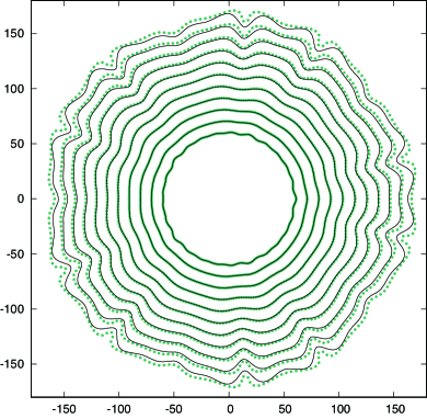
(a)

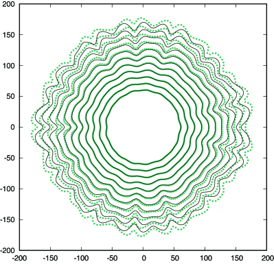
(b)

Figure 2: Comparison results for (1) using our scheme §4.1 and for (2) using the method proposed in GKY . (a): $p_{i}=0.12\cdot i$, $m_{i}=5(1+i)$; (b): $p_{i}=0.06\cdot i$, $m_{1}=7$, $m_{2}=11$, $m_{3}=13$, $m_{4}=17$;

From Fig. 2, for the perturbation part, it is experimentally confirmed that the behavior of the graph and interface are almost the same. Therefore, we confirm that it is reasonable to use the graph (1) to theoretically analyze the qualitative properties of the solution to the interfacial equation (2). There is a difference in the behavior when a sufficient amount of time has been spent, which may indicate the limitation in that the graph cannot be overhang.

4.3 Wavenumber selection and parameters (theoretical results)

In this subsection only, let $R(t)$ be the bifurcation parameter $R$. Then, the neutral stability curves upon which the linearized operator

$$\mathcal{L} =\dfrac{\delta}{R^{4}}\dfrac{\partial^{4}}{\partial\sigma^{4}}+\dfrac{1}{R^{2}}\left(\alpha-1+\dfrac{\delta}{R^{2}}\right)\dfrac{\partial^{2}}{\partial\sigma^{2}}+\dfrac{\alpha-1}{R^{2}}$$

corresponding to (1) has eigenvalues of zero around the circle solution are defined as follows (see Fig. 3):

Definition 1 (Definition 2 in KUY )

The neutral stability curves are defined as a set of parameters

$$\left\{(R,\delta);\,\delta=\dfrac{\alpha-1}{m^{2}}R^{2},\ m\in\mathbb{Z}\right\}$$ (60)

upon which $\mathcal{L}$ has eigenvalues of zero.

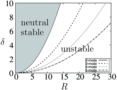
Figure 3: The $|m|$-mode neutral stability curves when $\alpha=1.2$ with $|m|=2,3,4,5$. The horizontal and vertical axes represent $R$ and $\delta$, respectively (KUY ).

From the above definition, we see that the circle solution is neutrally stable as in the gray region, whereas in the white region where $R>R^{*}:=2\sqrt{\delta/(\alpha-1)}$, the circle solution is unstable except at the 2-mode neutral stability curve because at least one eigenvalue is positive (for details, see Appendix A). According to this definition, as long as $|\alpha-1|$ is sufficiently small, we can know the relationship between the wavenumber of the solution to (2) and the parameters. Therefore, to study the qualitative properties of the solution for (2), it is important to study the instability of the solution for (1).

4.4 Wavenumber selection and parameters (numerical results)

In this subsection, we show that the maximum wavenumber of the unstable mode can be identified a priori by appropriately choosing the parameters and initial radius. The parameters are $dt=0.01$, $N=1024$, $T=100$, $v_{c}=0.001$, $\alpha=1.5$, $\delta=4.0$, and $p_{i}=0.1$ for the initial conditions (59). In Figs. 4–8, (a), (b), and (c) show (58) at $t=0,20,\dots,100$, the numerical solution $u(\sigma,t)$, and $R(t)$ in the parameter space $(R,\delta)$ (see KUY ), respectively. In (b) of the figures, the solid lines are the numerical solution $u(\sigma,T)$, and the dashed lines are the initial data $u(\sigma,0)$. The curves in (c) are called neutral stability curves $\delta=\dfrac{\alpha-1}{m^{2}}R^{2}$ $(m\in\mathbb{N}\setminus\{1\})$, upon which the linearized operator around the trivial solution $u(\sigma,t)\equiv 0$ has at least one eigenvalue of zero.

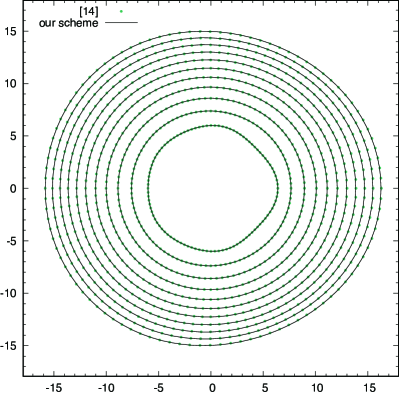
(a)

(b)

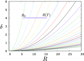
(c)

Figure 4: Numerical results for the case in which $R_{0}=6.0$ and $(m_{1},m_{2},m_{3},m_{4})=(2,3,4,5)$ in (59).

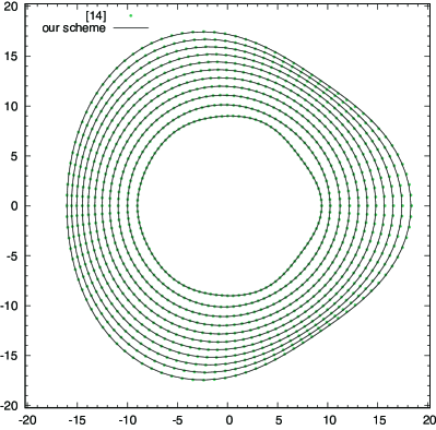
(a)

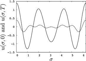
(b)

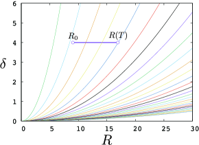
(c)

Figure 5: Numerical results for the case in which $R_{0}=9.0$ and $(m_{1},m_{2},m_{3},m_{4})=(3,4,5,6)$ in (59).

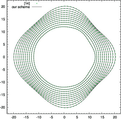
(a)

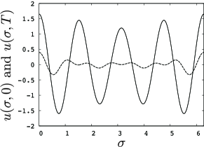
(b)

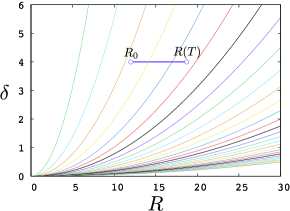
(c)

Figure 6: Numerical results for the case in which $R_{0}=12.0$ and $(m_{1},m_{2},m_{3},m_{4})=(4,5,6,7)$ in (59).

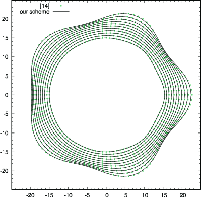
(a)

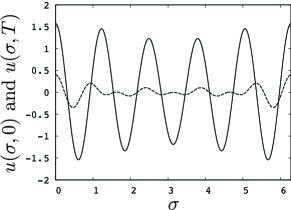
(b)

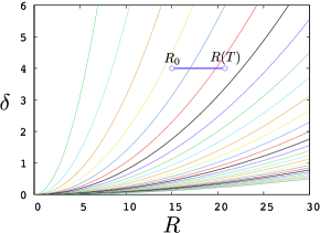
(c)

Figure 7: Numerical results for the case in which $R_{0}=15.0$ and $(m_{1},m_{2},m_{3},m_{4})=(5,6,7,8)$ in (59).

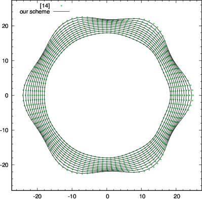
(a)

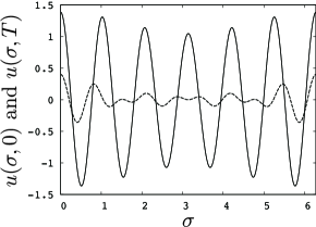
(b)

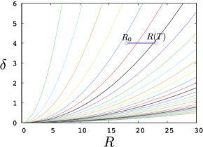
(c)

Figure 8: Numerical results for the case in which $R_{0}=18.0$ and $(m_{1},m_{2},m_{3},m_{4})=(6,7,8,9)$ in (59).

5 Concluding remarks

In the present paper, we proposed a simple, fast, and accurate numerical scheme for the KS equation (1) defined on an expanding circle. Our scheme is the Crank–Nicolson type finite difference scheme of (4) (the differential form of (1)), and we demonstrated the existence, uniqueness, and second-order convergence. To the best of our knowledge, with the exception of our graph approach, there are no convergence results of the numerical scheme for the interfacial equation (2) in a parametric approach or a level set approach.

As mentioned above, our scheme is fast because the time increment $k$ can be taken, such as $k=o(h^{\frac{1}{4}})$, in comparison with the standard increment $k=O(h^{4})$ for an explicit scheme (see Theorem 2.2). In addition, our scheme is more accurate than the numerical method of (2) as long as the amplitude of the solution is sufficiently small because the experimental order of convergence (the so-called EOC) of the numerical method is $1$ (see KKUYB ).

Owing to the derivation of the equations (1), if $\alpha$ is sufficiently small, it is expected to be a good approximation of the solution to the original interfacial equation (2). Indeed, in subsection 4.4, we can see that the wavenumbers of the numerical solutions of (2) and (1) are consistent. Therefore, we insist that our model (1) captures well the instability of the solution to the interfacial model. In other words, we can determine a priori the unstable mode of the maximum wavenumber by choosing the parameters and initial radius regarding the parameter space of $(R,\delta)$ (see Fig. 3).

By contrast, as shown in Fig. 2, the green points (numerical solutions to (2)) are eventually separated from the solid lines (numerical solutions to (1)). As the reason for such separation, the self-intersection of the moving curves is allowed in the interfacial model, whereas it cannot occur in our graph model. This observation suggests that a finite-time blow-up occurs for a solution $v(\sigma,t)=u_{\sigma}(\sigma,t)$. An analysis of the blow-up phenomenon remains as one of our future studies.

Appendix A Neutral stability curves

In this section, we describe a linearized stability analysis of (1) around the trivial solution $u(\sigma,t)\equiv 0$. Substituting the Fourier expansion $u(\sigma,t)=\sum_{m\in\mathbb{Z}}u_{m}(t){\mathrm{e}}^{\sqrt{-1}m\sigma}$, $u_{m}(\cdot)\in\mathbb{C}$ into (1), we obtain an infinite-dimensional dynamical system:

$$\dot{u}_{m}(t)=\lambda_{m}u_{m}(t)-\dfrac{v_{c}}{2R^{2}}\sum_{\begin{subarray}{c}m_{1}+m_{2}=m\\ m_{1}m_{2}\neq 0\end{subarray}}m_{1}m_{2}u_{m_{1}}(t)u_{m_{2}}(t),$$ (61)

where $\lambda_{\pm 1}\equiv 0$ and

$$\lambda_{|m|\geq 2}=-\dfrac{\delta m^{4}}{R^{4}}+\dfrac{m^{2}}{R^{2}}\left(\alpha-1+\dfrac{\delta}{R^{2}}\right)-\dfrac{\alpha-1}{R^{2}}.$$

Note that $u_{-m}(t)=\bar{u}_{m}(t)$ follows from $u(\cdot,\cdot)\in\mathbb{R}$. By solving $\lambda_{m}=0$ on $R$, we obtain the neutral stability curves upon which the linearized operator of (1) has eigenvalues of zero. Note that $\lambda_{\pm 1}\equiv 0$ holds for any $R>0$. However, $\lambda_{m}<0$ holds for each $|m|=2,3,\cdots$ when $R<R_{*}=2\sqrt{\delta/(\alpha-1)}$. Therefore, the circle solution is neutrally stable as indicated in the gray region in Fig. 3. In the white region where $R>R_{*}$, the circle is unstable except at the $2$-mode neutral-stability curve because $\lambda_{m}>0$ holds for at least one integer $m\in\{\pm 2,\pm 3,\dots\}$. In particular, when $|m|=2$, for any fixed $\delta>0$, the value of $R_{*}$ is the minimum value at which the stability of the circle solution changes from neutrally stable to unstable.

References

- (1) G. D. Akrivis, Finite difference discretization of the Kuramoto–Sivashinsky equation, Numer. Math., 63, 1–11 (1992).
- (2) G. D. Akrivis, Finite element discretization of the Kuramoto–Sivashinsky equation, Numer. Analysis and Mathematical Modeling, 29, 155–163 (1994).
- (3) D. M. Ambrose & A. L. Mazzucato, Global existence and analyticity for the 2D Kuramoto–Sivashinsky equation, J. Dyn. Diff. Equat., 31(3), 1525–1547 (2019).
- (4) D. Armbruster, J. Guckenheimer and P. Holmes, Heteroclinic cycles and modulated travelling waves in systems with O(2) symmetry, Physica D, 29, 257–282 (1988).
- (5) D. Armbruster, J. Guckenheimer and P. Holmes, Kuramoto–Sivashinsky dynamics of the center-unstable manifold, SIAM J. Appl. Math., 49(3), 676–691 (1989).
- (6) F. E. Browder, Existence and uniqueness theorems for solutions of nonlinear boundary value problems, Proceedings of symposia in applied mathematics, 17, 24–49 (1965).
- (7) H. Bhatt & A. Chowdhury, A compact fourth-order implicit-explicit Runge–Kutta type scheme for numerical solution of the Kuramoto–Sivashinsky equation, arXiv.
- (8) M. Beneš, J. Kratochvíl, J. Křištan, V. Minárik and P. Pauš, A parametric simulation method for discrete dislocation dynamics, Eur. Phys. J-Spec. Top., 177, 177–192 (2009).
- (9) C. L. Epstein & M. Gage, The curve shortening flow, Wave motion: theory, modelling, and computation, Math. Sci. Res. Inst. Publ., 7, 15–59 (1987).
- (10) A. Fasano, M. Mimura and M. Primicerio, Modelling a slow smoldering combustion process, Math. Methods Appl. Sci., 33, 1211–1220 (2009).
- (11) M. L. Frankel & G. I. Sivashisnky, On the nonlinear thermal diffusive theory of curved flames, J. Phys., 48, 25–28 (1987).
- (12) M. Goto, K. Kuwana, K. Kushida and S. Yazaki, Experimental and theoretial study on near-floor flame spread along a thin solid, Proceedings of the Combustion Institute, 37, 3783–3791 (2019).
- (13) M. Goto, K. Kuwana, Y. Uegata and S. Yazaki, A method how to determine parameters arising in a smoldering evolution equation by image segmentation for experiment’s movies, DCDS S, 14, 881–891 (2021).
- (14) M. Goto, K. Kuwana and S. Yazaki, A simple and fast numerical method for solving flame/smoldering evolution equations, JSIAM Lett., 10, 49–52 (2018).
- (15) J. M. Hyman & B. Nicolaenko, The Kuramoto–Sivashinsky Equation: A bridge between PDE’S and dynamical systems, Physica D, 18, 113–126 (1986).
- (16) E. R. Ijioma, H. Izuhara, M. Mimura and T. Ogawa, Homogenization and fingering instability of a microgravity smoldering combustion problem with radiative heat transfer, Combust. Flame, 162, 4046–4062 (2015).
- (17) E. R. Ijioma, H. Izuhara, M. Mimura and T. Ogawa, Computational Study of Nonadiabatic Wave Patterns in Smoldering Combustion under Microgravity, East Asian Journal of Applied Mathematics, 5, 138–149 (2015).
- (18) K. Ikeda & M. Mimura, Mathematical treatment of a model for smoldering combustion, Hiroshima Math. J., 38, 349–361 (2008).
- (19) K. Ikeda & M. Mimura, Traveling wave solutions of a 3-component reaction-diffusion model in smoldering combustion, Commun. Pure Appl. Anal., 11, 275–305 (2012).
- (20) M. Kolář, S. Kobayashi, Y. Uegata, S. Yazaki and M. Benes, Analysis of Kuramoto–Sivashinsky Model of Flame/Smoldering Front by Means of Curvature Driven Flow, Numerical Mathematics and Advanced Applications ENUMATH 2019, 615–624 (2021).
- (21) L. Kagan & G. I. Sivashinsky, Pattern formation in flame spread over thin solid fuels, Combust. Theory Model., 12, 269–281 (2008).
- (22) K. Kuwana, K. Suzuki, Y. Tada and G. Kushida, Effective Lewis number of smoldering spread over a thin solid in a narrow channel, Proceedings of the Combustion Institute, 36, 3203–3210 (2017).
- (23) Y. Kuramoto & T. Tsuzuki, Persistent propagation of concentration waves in dissipative media far from thermal equilibrium, Progr. Theor. Phys., 55, 356–369 (1976).
- (24) S. Kobayashi, Y. Uegata and S. Yazaki, The existence of intrinsic rotating wave solutions of a flame/smoldering-front evolution equation, JSIAM Lett., 12, 53–56 (2020).
- (25) D. M. Michelson & G. I. Sivashinsky, Nonlinear analysis of hydrodynamic instability in laminar flames–II. Numerical experiments, Acta Astronautica, 4, 1207–1221 (1977).
- (26) B. Nicolaenko & B. Scheurer, Remarks on the Kuramoto–Sivashinsky equation, Physica D, 12, 391–395 (1984).
- (27) B. Nicolaenko, B. Scheurer and R. Temam, Some global dynamical properties of the Kuramoto–Sivashinsky equations: nonlinear stability and attractors, Physica D, 16(2), 155–183 (1985).
- (28) S. L. Olson, H. R. Baum and T. Kashiwagi, Finger-like smoldering over thin cellulosic sheets in microgravity, Proc. Combust. Inst., 27, 2525–2533 (1998).
- (29) J. Porter & E. Knobloch, New type of complex dynamics in the 1:2 spatial resonance, Physica D, 159, 125–154 (2001).
- (30) D. T. Pagageorgiou & Y. S. Smyrlis, The Route to Chaos for the Kuramoto–Sivashinsky Equation, Theoret. Comput. Fluid Dynamics, 3, 15–42 (1991).
- (31) J. C. Robinson, Inertial manifolds for the Kuramoto–Sivashinsky equation, Physics Letters A, 184, 190–193 (1994).
- (32) G. I. Sivashinsky, Nonlinear analysis of hydrodynamic instability in laminar flames-I, Acta Astron., 4, 1177–1206 (1977).
- (33) G. I. Sivashinsky & D. M. Michelson, On Irregular Wavy Flow of a Liquid Film Down a Vertical Plane, Prog. Theor. Phys., 63, 2112–2114 (1980).
- (34) D. Ševčvič & S. Yazaki, On a gradient flow of plane curves minimizing the anisoperimetric ratio, IAENG International J. Appl. Math., 43, 160–171 (2013).
- (35) E. Tadmor, The well-posedness of the Kuramoto–Sivashisnky equation, SIAM J. Math. Anal., 17(4), 884–893 (1986).
- (36) O. Zik, Z. Olami and E. Moses, Fingering instability in combustion, Phys. Rev. Lett., 81, 3868–3871 (1998).
- (37) O. Zik & E. Moses, Fingering instability in solid fuel combustion: the characteristic scales of the developed state, Proc. Combust. Inst., 27, 2815–2820 (1998).
- (38) O. Zik & E. Moses, Fingering instability in combustion: an extended view, Phys. Rev. E, 60, 518–531 (1999).
- (39) Y. Zhang, P. D. Ronney, E. V. Roegner and B. Greenberg, Lewis Number Effects on Flame Spreading Over Thin Solid Fuels, Combust. Flame, 90, 71–83 (1992).