Congested Crowd Instance Localization with Dilated Convolutional Swin Transformer

Abstract

Crowd localization is a new computer vision task, evolved from crowd counting. Different from the latter, it provides more precise location information for each instance, not just counting numbers for the whole crowd scene, which brings greater challenges, especially in extremely congested crowd scenes. In this paper, we focus on how to achieve precise instance localization in high-density crowd scenes, and to alleviate the problem that the feature extraction ability of the traditional model is reduced due to the target occlusion, the image blur, etc. To this end, we propose a Dilated Convolutional Swin Transformer (DCST) for congested crowd scenes. Specifically, a window-based vision transformer is introduced into the crowd localization task, which effectively improves the capacity of representation learning. Then, the well-designed dilated convolutional module is inserted into some different stages of the transformer to enhance the large-range contextual information. Extensive experiments evidence the effectiveness of the proposed methods and achieve the state-of-the-art performance on five popular datasets. Especially, the proposed model achieves F1-measure of 77.5% and MAE of 84.2 in terms of localization and counting performance, respectively.

I Introduction

Recently, crowd localization is a hot topic in the field of crowd analysis due to more accurate prediction results than other tasks, such as crowd counting [1, 2, 3, 4, 5] and flow estimation [6, 7]. It takes individuals in the crowd scene as the basic unit instead of the scenes. Instance-level localization yields each person’s position, which may assist other crowd analysis semantic tasks, trajectory prediction [8], anomaly detection [9, 10], video summarization [11, 12], group detection [13, 14, 15], etc. Accurate head localization is important for tracking it, predicting its trajectory, recognizing its action and other high-level tasks. Thus, crowd localization is also a fundamental task in crowd analysis.

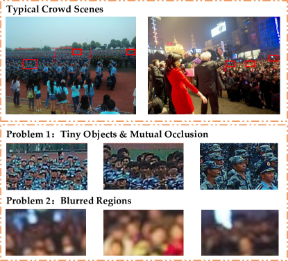
Figure 1: Two problems in some typical crowd scenes: Tiny Objects & Mutual Occlusion and Blurred Regions, which cause that the current crowd localization models perform poorly in dense crowd scenes.

I-A Motivation

Currently, there are many researchers focus on crowd localization task. Benefited from the development of the object detection and localization [16, 17], some methods are proposed for person/head/face detection in sparse scenes, namely low-density crowds. Representative algorithms are DecideNet [18], TinyFaces [19], and so on. To handle the dense crowds, some methods [20, 21] exploit point supervision to train a locator. Unfortunately, they perform not well for large-scale heads because of a lack of scale information. To reduce the scale-invariant problem, Gao et al. [22] propose a segmentation-based localization framework, which treats each head as a non-overlapped instance area and directly outputs its independent semantic head region.

However, in extremely congested scenes, the traditional models can not work well. The main reasons are: 1) small-scale objects and mutual occlusion lack detailed appearance; 2) blurred crowd regions lead to missing the structured patterns of faces. This situation generally occurs at the far end of the shooting angle of view. Fig. 1 demonstrates the aforementioned issues using two typical crowd scenes. For alleviating these two problems, this paper proposes a high-capacity Dilated Convolutional Swin Transformer (DCST) for instance localization in the extremely congested crowd scenes. For the first problem, we exploit a popular vision transformer, Swin Transformer (ST) [23], to encode richer features than traditional CNN. Then by re-organizing the feature to spatial level, the model can output independent instance map (IIM) [22]. Finally, the FPN decoder [24] is added to ST to produce a segmentation map with the same size as input.

For the second problem, we present a method of modeling the context is used to assist in estimating instance locations in the blurred regions. Although Swin Transformer adopts shifted window to enlarge respective fields in different layers, we find that ST+FPN also performs poorly. The effect of this operation on the encoding of context information is limited. Thus, we attempt to add traditional dilated convolutional layers to the different stages in Swin Transformer, named as “Dilated Convolutional Swin Transformer”, DCST for short. Specifically, the dilatation module is designed, which consists of two convolutional layers with the dilated rate 2 and 3, respectively. After a stage in the transformer, the features are re-ordered like CNN’s feature map. Then by a proposed dilatation module, the large-range contextual information is successfully encoded. Finally, the feature map is recalled with the original size and fed into the next stage in the transformer. Compared with the original Swin Transformer, DCST has a larger respective field and can learn contextual information more effectively.

I-B Contributions

In summary, the contributions of this paper are three-fold:

1. Propose an effective framework for crowd localization, consisting of a vision transformer as the encoder and an FPN as the decoder.

2. Design a flexible dilatation module and insert it in the transformer encoder, which prompts the contextual encoding capability.

3. The proposed DCST achieves the state-of-the-art performance on the six benchmark or datasets, NWPU-Crowd, JHU++, UCF-QNRF, ShanghaiTech A/B, and FDST.

I-C Organization

The rest of this paper is organized as follows. Section II briefly lists and reviews the related literature and works about crowd localization and transformer. Then, Section III describes the proposed Dilated Convolutional Swin Transformer (DCST) framework for independent instance segmentation and network architecture. Further, Section IV conducts the extensive experiments, and Section V further analysis the key settings of the method. Finally, this work is summarized in Section VI.

II Related Works

In this section, the related works about crowd localization and vision transformer are briefly reviewed.

II-A Crowd Localization

Detection-based models     In the early days, few methods directly focus on individual localization in crowd scenes. Most algorithms try to detect pedestrians, heads, faces, etc. in natural images. Specifically, Liu et al. [25] propose a segmentation-based method to detect individuals in Surveillance Applications. Andriluka et al. [26] present a non-rigid object detection framework, which is based on pictorial structures model [27] and strong part detectors [28] for people detection. Considering the occlusion problem in crowded scenes, some methods focus on detecting the head to locate each individual. Rodriguez et al. [29] propose a density-aware head detection algorithm, which effectively leverages information on the scene’s global structure and resolved all detections. Van et al. [30] design a template matching method using point cloud data for head detection. Stewart and Andriluka [31] present an end-to-end detector based on OverFeat [32] to locating the head position. In addition to the person and head localization algorithms, some detection methods aim to detect tiny faces in dense crowds. Hu and Ramanan [19] propose a tiny face detection method, which explores the impacts of image resolution, face scale, etc. Li et al. [33] design a context-based module in face detector and propose a data augmentation strategy (Data-anchor-sampling) to prompt the performance. Deng et al. [34] annotate five landmarks for each face to improve the performance of hard sample localization.

Point-based models     The aforementioned detection-based methods are not suitable for dense crowd scenes, especially when there are more than 1,000 people. Before 2020, the common congested crowd datasets do not provide box-level annotations. Thus, some point-based methods are very popular in this field. Idrees et al. [35] attempt to find the peak point in the predicted density maps. By locating the maximum value in a local region, the head position is obtained. Liu et al. [36] propose a new label type, Cruciform, which easier to be located maximum value than traditional density maps. Gao et al. [37] design an iterative scheme to find maximum values in reverse for density maps. Wan and Chan [38] present a new method to construct the noises of point annotations, which enhances the robustness of the crowd model. Wang et al. [21] present a self-training mechanism based on a key-point detector to predict the head center. Wang et al. [39] construct a baseline for crowd localization based on a point-based detection method [40]. Sam et al. [20] propose a detector tailor-made for dense crowds only relying on pseudo box labels generated by point information. Liang et al. [41] design a Focal Inverse Distance Transform map to depict labels, and propose an I-SSIM loss to detect local Maxima. Wan et al. [5] propose a generalized loss function to learn robust density maps for counting and localization simultaneously.

Segmentation-based models     With the release of high-resolution datasets, NWPU-Crowd [42], segmentation-based methods attract many researchers’ attention. Abousamra et al. [43] propose a topological constraint to model the spatial arrangement, which uses a persistence loss based on the persistent homology. Gao et al. [44] propose an adaptive threshold module to elaborately segment tiny heads in dense crowd regions. Considering that segmentation maps provide a more refined and reasonable label, this paper will be based on it to deploy our works.

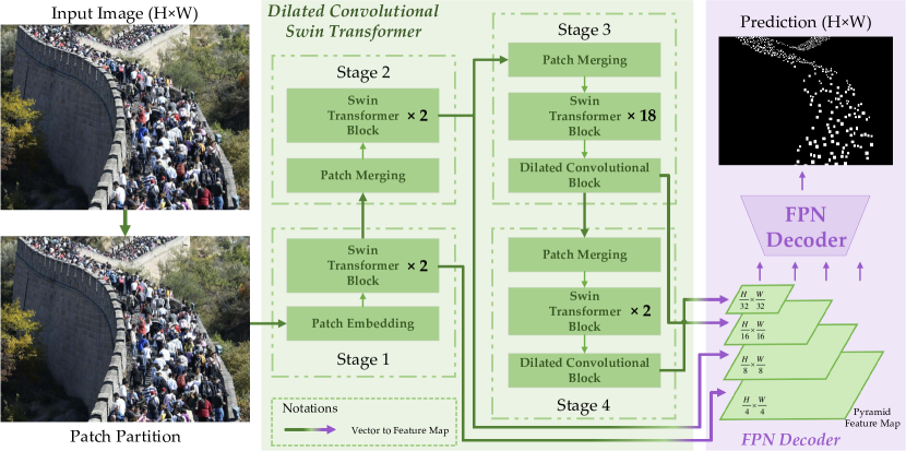
Figure 2: The flowchart of the proposed Dilated Convolutional Swin Transformer and FPN decoder (DCST+FPN). Notably, In Stage 3 and 4, the Dilated Convolutional Block (DCB) is applied to the top of the Swin Transformer Block (STB). By a Feature Pyramid Networks (FPN) decoder, the features from different stages are fused, and the final independent instance segmentation map with the input size is produced.

II-B Vision Transformer

Transformer is proposed by Vaswani et al. [45]. It is widely used in many NLP tasks due to its powerful feature extraction capacity. In 2020, Dosovitskiy et al. [46] propose a vision transformer (ViT) for image recognition, which shows the high-performance representation learning ability in computer vision tasks. After this, many vision transformer variants are presented. Yuan et al. [47] present a Tokens-to-Token ViT (T2T ViT), which can encode the local structures for each token. Wang at al. [48] propose a backbone transformer for dense prediction, named as “Pyramid Vision Transformer (PVT)”,which designs a shrinking pyramid scheme to reduce the traditional transformer’s sequence length. Han et al. [49] propose a Transformer-iN-Transformer (TNT) architecture, of which the inner extracts local features, and the outer processes patch embeddings. To achieve a trade-off between speed and accuracy, Liu et al. [23] introduce a shifted window strategy into transformer to encode representations. In the field of crowd analysis, Liang et al. [50] propose a transformer for weakly-supervised counting, which exploits a transformer to directly regress the number of counting. Sun et al. [51] design a token-attention module to encode features by channel-wise attention, and a regression-token module to produce the count of people in crowd scenes.

III Approach

This section firstly reviews the basic Vision Transformer (ViT) and its variants Shift Window ViT (ST). Then we describe the proposed Dilated Convolutional Shift Window ViT (DCST). Finally, the network architecture, loss function, and implementation details are reported.

III-A Vision Transformer (ViT)

At present, vision transformer shows its powerful capacity of representation learning. In 2017, transformer is proposed by Vaswani et al. [45] and become a standard operation in the field of Natural Language Processing (NLP). Notably, BERT [52] and GPT [53] obtain remarkable progress in the related tasks. Carion et al. [54] exploit transformer to detect objects, which is added to the top of traditional CNNs. Dosovitskiy et al. [46] propose a fully transformer architecture for image classification, named as “Vision Transformer (ViT)”. Here, we briefly review ViT.

III-A1 Patch embeddings

Given an image $i\in{\mathcal{R}^{H\times W\times C}}$ with the size of height $H$, width $W$ and channel $C$ , it is reshaped into a sequence, which consists of $N$ ($N={{HW}\mathord{\left/{\vphantom{{HW}{{P^{2}}}}}\right.\kern-1.2pt}{{P^{2}}}}$) patches ${i_{p}}$ with the size of $P\times P\times C$. Then each patch is flattened and mapped to $D$ dimensions latent vector using a trainable linear projection in transformer, of which output is named as “patch embeddings”. In addition, position embeddings ${\bm{E}_{pos}}$ are added to the patch embeddings to represent positional information, which are learnable 1D embeddings. Finally, The sequence of embedding vectors are fed into the Transformer Encoder.

Specifically, the operation of patch embeddings is formulated as follows:

$$\begin{array}[]{l}\begin{aligned} {z_{0}}=[{i_{class}};\;i_{p}^{1}\bm{E};\;i_{p}^{2}\bm{E};\;...;\;i_{p}^{N}\bm{E}]+{\bm{E}_{pos}},\end{aligned}\end{array}$$ (1)

where ${i_{class}}$ is the embedded patches $z_{0}^{0}$, and $\bm{E}$ denotes the process of the learnable embeddings ($\bm{E}\in{R^{({P^{2}}\times C)\times D}}$, $\bm{E}\in{R^{(N+1)\times D}}$).

III-A2 Transformer Encoder

Transformer Encoder includes Multi-headed Self-Attention (MSA) and Multi-Layer (MLP) modules. Given a $L$ layers of Transformer Encoder, MSA and MLP are formulated as:

$$\begin{array}[]{l}\begin{aligned} z_{l}^{\prime}=MSA(LN({z_{l-1}}))+{z_{l-1}},\quad l=1,...,L,\end{aligned}\end{array}$$ (2)

$$\begin{array}[]{l}\begin{aligned} {z_{l}}=MLP(LN(z_{l}^{\prime}))+z_{l}^{\prime},\quad l=1,...,L,\end{aligned}\end{array}$$ (3)

where LN denotes Layer Normalization [55] for stable training. In MLP, two layers with GELU non-linearity activation function [56] are applied. Notably, LN is employed for each sample $z$:

$$\begin{array}[]{l}\begin{aligned} LN(z)=\frac{{z-\mu}}{\delta}\circ\gamma+\beta,\end{aligned}\end{array}$$ (4)

where $\mu$ and $\delta$ denote the mean and standard deviation of features respectively, $\gamma$ and $\beta$ are the learnable parameters of affine transformation, and $\circ$ is element-wise dot operation.

III-B Swin Transformer

Compared with ViT, Swin Transformer is a hierarchical architecture for handling dense prediction problems and reducing the computational complexity. Specifically, it computes self-attention in non-overlapping windows with small-scale sizes. Further, to encode contextual information, the window partitions in consecutive layers are different. Consequently, the large-range information is transformed in the entire network by local self-attention modules.

Swin Transformer contains four stages to produce different number tokens. Given an image with the size of $H\times W$, token is a raw pixels concatenation vector of an RGB image patch with the size of $4\times 4$. A linear embedding is employed on this token to map it into a vector with the dimension $C$. Stage 1, 2, 3, and 4 produce $\frac{H}{4}\times\frac{W}{4}$, $\frac{H}{8}\times\frac{W}{8}$, $\frac{H}{16}\times\frac{W}{16}$, and $\frac{H}{32}\times\frac{W}{32}$ tokens, respectively. Each stage consists of a Patch Embedding and some Swin Transformer Blocks. Different from MSA in ViT, a Swin Transformer Blocks uses the shifted-window MSA to compute locally self-attention.

III-C Dilated Convolutional Swin Transformer

Although Swin Transformer design a shifted-widow scheme of the sequential layers in a hierarchical architecture, large-range spatial contextual information is still encoded not well. For alleviating this problem, we propose a Dilated Convolutional Swin Transformer (“DCST” for short) to enlarge the respective field for spatial images. In this way, the large-range contextual information can be encoded well on different scales. To be specific, the Dilated Convolutional Block is designed and inserted into between different stages of Swin Transformer.

Dilated Convolution     Dilated Convolution is proposed by Yu and Koltun [57] in 2015. Compared with the traditional convolution operation, the dilated convolution supports the expansion of the receptive field. Notably, a traditional $3\times 3$-kernel convolution has a respective field of $3\times 3$. If it is a 2-dilated convolution with the same kernel size, the respective field is $7\times 7$. Thus, the dilated convolution can expand the respective field without loss of feature resolution.

Dilated Convolutional Block (DCB)     Considering that the data flow in Swin Transformer is vectors instead of feature maps in traditional CNNs, DCB firstly reshapes a group of vector features into a spatial feature map. For example, the number of $\frac{H}{4}\times\frac{W}{4}$ $C$-dimension tokens is reshaped as a feature map with the size of $\frac{H}{4}\times\frac{W}{4}\times C$. After this, two dilated convolutional with Batch Normalization [58] and ReLU are applied to extract large-range spatial features. Finally, the feature map is re-transformed the original number and size (namely the number of $\frac{H}{4}\times\frac{W}{4}$ $C$-dimension tokens) and fed into the next stage in Swin Transformer.

III-D Network Configurations

For the dense prediction task, a classic architecture is an Encoder-Decoder network to output results with the same size of the inputs. In this paper, the encoder is the proposed DCST and the decoder is based on FPN [59].

Encoder: DCST     In DCST, the Swin Transformer is Swin-B, of which four stages has 2, 2, 18, and 2 Swin Transformer Blocks. After Stage 3 and 4, the Dilated Convolutional Block (DCB) is added. Following by [60], the dilatation rate of the two dilated convolutional layers in DCB is $2$ and $3$.

Decoder: FPN     Similar to IIM [22], this paper also utilizes FPN [59] to fuse different-scale features. To be specific, for DCST’s four stages, the four-head FPN is designed. Finally, for a high-resolution output to obtain an independent instance map, a convolutional layer and two de-convolutional layers is applied to yields the $1$-channel feature map with the original input size. A sigmoid activation is employed to normalize the results in $(-1,1)$, which is named as “score map”.

III-E Loss Function

For training the crowd localization model, we adopt the standard Mean Squared Error (MSE) loss function.

III-F Implementation Details

Training Setting      For augmenting the data, random horizontally flipping, random scaling (target scales: $0.8\times\sim 1.2\times$ original scales) and random cropping (target size: 512px $\times$ 1024px) are employed. The experiments are conducted on two NVIDIA TITAN RTXs ($\sim$48GB GPU Memory) The batch size is $8$. The base learning rate of transformer and FPN is set as $0.6\times{10^{-5}}$, and the dilated conv layers’ base learning rate is set as $0.6\times{10^{-6}}$. A linear warmup is implemented in first 1,500 iterations. AdamW [61] algorithm is utilized to optimize the proposed network.

Threshold Selection      For the score map yielded by the network, we need to select a proper threshold to transform it into a binary map. The purpose is that each independent instance can be detected by connected component segmentation. Notably, the best threshold is selected on the validation set and is directly applied on the test set.

IV Experimental Results

The experiments are conducted on six main-stream crowd datasets, including NWPU-Crowd, JHU-CROWD++, FDST, UCF-QNRF, and ShanghaiTech Part A/B Dataset. At the same time, the further analyses are discussed in Section V on the NWPU-Crowd validation set.

IV-A Evaluation Criteria

Crowd Localization     In this section, we follow NWPU-Crowd [42] to evaluate instance-level Precision, Recall, and F1-measure (Pre., Rec., and F1-m for short in the following tables), which are calculated under the adaptive scale for each head. To be specific, the definitions of the above are:

$$\begin{array}[]{l}\begin{aligned} precision=\frac{{TP}}{{TP+FP}},\end{aligned}\end{array}$$ (5)

$$\begin{array}[]{l}\begin{aligned} recall=\frac{{TP}}{{TP+FN}},\end{aligned}\end{array}$$ (6)

$$\begin{array}[]{l}\begin{aligned} {F_{1}}=\frac{{\left({{\beta^{2}}+1}\right)\cdot precision\cdot recall}}{{{\beta^{2}}\cdot precision+recall}},\quad\beta=1,\end{aligned}\end{array}$$ (7)

where TP, FP, FN denote the number of True Positive, False Positive, and False Negative, respectively. The TP, FP, and FN is calculated under large $\sigma$, namely the radius of circumcircle for a head box label.

Crowd Counting     In addition to the metrics for localization, we also evaluate the counting performance using Mean Absolute Error (MAE), Mean Squared Error (MSE), and mean Normalized Absolute Error (NAE), which are defined as:

$$\begin{array}[]{l}\begin{aligned} MAE=\frac{1}{N}\sum\limits_{i=1}^{N}{\left|{{y_{i}}-{{\hat{y}}_{i}}}\right|}\end{aligned}\end{array}$$ (8)

$$\begin{array}[]{l}\begin{aligned} MSE=\sqrt{\frac{1}{N}\sum\limits_{i=1}^{N}{{{\left|{{y_{i}}-{{\hat{y}}_{i}}}\right|}^{2}}}},\end{aligned}\end{array}$$ (9)

$$\begin{array}[]{l}\begin{aligned} NAE=\frac{1}{N}\sum\limits_{i=1}^{N}{\frac{\left|{{y_{i}}-{{\hat{y}}_{i}}}\right|}{{y_{i}}}},\end{aligned}\end{array}$$ (10)

where N is the number of samples in test or validation set, $y_{i}$ is GT number and ${{{\hat{y}}_{i}}}$ is predicted number for $i$-th sample.

IV-B Datasets

NWPU-Crowd [42] is a large-scale high-quality and high-resolution crowd counting and localization dataset, consisting of 5,109 scenes and 2,133,238 instances. It provides two types of annotation, point-level and box-level for each head.

JHU-CROWD++ [62] is an extension version of JHU-CROWD [63], which consists of 4,372 images, $\sim$1.5 million instances. It contains high-diversity crowd scenes, such as rain, snow, haze, etc. For each head, the point level, approximate size, blur level, occlusion level are labeled.

FDST [64] is a video crowd counting dataset, which consists of 13 different scenes, 100 image sequences, 150,000 frames. It also annotates point-level and box-level labels simultaneously.

UCF-QNRF is proposed by Idrees et al. [35], which is a congested crowd counting dataset, consisting of 1,535 dense scenes, with a total of 1,251,642 instances. The average of counting number is $\sim 815$.

Shanghai Tech is proposed by Zhang et al. [65] , which has two subsets, Part A and B. The former labels 482 images, 241,677 instances; the latter has 716 images, including 88,488 labeled heads.

Note that UCF-QNRF and Shanghai Tech datasets do not provide the head scale. Following Gao et al. [22], we adopt the predicted scale information to evaluate the performance for localization. The generation code for scale information is available at https://github.com/taohan10200/IIM.

IV-C Ablation Study on the NWPU-Crowd validation set

To further understand each component in the proposed method, this section compares the step-wise results on the NWPU-Crowd validation set.

ST: A crowd counting model. Swin Transformer for image recognition model. The last classification layer is replaced by a sigmoid layer to directly output the number of people in crowd scenes.

DCST: A crowd counting model. Dilated Convolutional Swin Transformer for image recognition model. Similarly, the last classification layer is replaced by a Sigmoid layer.

ST+base decoder: A crowd counting and localization model. Swin Transformer is used as a backbone to extract features. The decoder is added to the top of Stage 4 in Swin Transformer, which consists of one convolutional layer and two de-convolutional layer output high-resolution score maps.

ST+FPN: Different from ST+base decoder, FPN decoder is employed to fuse the outputs of four stages in Swin Transformer and to output high-quality score maps.

DCST+FPN: Compared with ST+FPN, the backbone is replaced by DCST.

TABLE I: Ablation study of different components in the proposed method on the NWPU-Crowd validation set.

Method	Localization			Counting
	F1-m	Pre	Rec	MAE	MSE	NAE
ST	-	-	-	103.2	393.2	0.307
DCST	-	-	-	96.3	412.0	0.248
ST+base decoder	73.7	80.1	68.2	77.5	324.0	0.193
ST+FPN	79.8	88.3	72.7	54.6	181.4	0.159
DCST+FPN	81.4	84.1	79.0	43.9	109.8	0.156

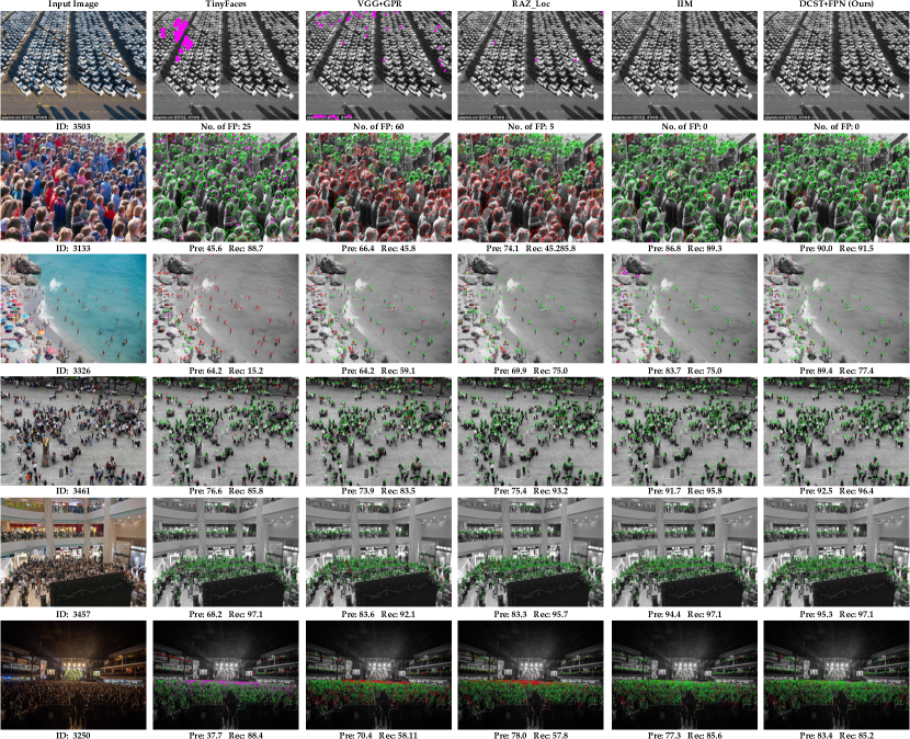
Figure 3: Six groups of visualization predicted results of four popular methods and the proposed DCST+FPN on NWPU-Crowd validation set. The showing contains Negative Samples (ID: 3503), large-scale heads (ID: 3133), tiny heads (ID: 3326 & 3461), dense crowds (ID: 3457 & 3250) and low-light scenes(ID: 3250). For a better visual effect, predicted images’ contents are shown by the gray scale, where green, red and magenta points denote true positive (TP), false negative (FN) and false positive (FP), respectively. Besides, the green and red circles are GroundTruth with the radius of $\sigma_{l}$.

Table I lists the performance of each model for localization and counting on the NWPU-Crowd validation set. Considering that ST and DCST directly output the number of people in crowd scenes, the localization metrics are not reported. From the table, the full model (DCST+FPN) achieves better performance (F1-measure of 81.4 and MAE of 43.9) than other baseline methods. From the overall trend, after the introduction of new modules, the performance is improved significantly. Besides, we find that pixel-wise-based methods have better results compared with scene-level-based algorithms (Row 3,4,5 v.s. Row 1,2). The former provides spatial annotations in the training process, but the latter only directly regresses a number. Therefore, Row 3,4,5’s methods learn more reasonable features than Row 1,2.

Effect of the DCB.   By comparing two groups of experiments (ST v.s. DCST and ST+FPN v.s. DCST+FPN), we find that introducing Dilated Convolutional Block (DCB) in Swin Transformer can effectively prompt the performance of localization and counting. Specifically, the estimation errors (MAE) increases by 6.7% and 19.6% for counting. At the same time, there is an interesting phenomenon that DCB is more effective in pixel-wise training than scene-level training (19.6% v.s. 6.7%), which evidences the dilated convolution captures the large-range contextual features for dense prediction tasks.

TABLE II: The leaderboard of NWPU-Crowd Localization (test set), excluding some anonymous submissions. The bold and underlined text denotes the first and second place, respectively. Avg.[B] of Recall means the average of recalls for different box level $[10^{0},10^{1}]$, $(10^{1},10^{2}]$, $(10^{2},10^{3}]$, $(10^{3},10^{4}]$, $(10^{4},10^{5}]$, and $>10^{5}$. The timestamp is Jun. 28, 2021, which is recorded in the official CrowdBenchmark website (the link is https://www.crowdbenchmark.com/historyresultl.html).

Method	Venue	Backbone	Overall ($\sigma_{l}$)		Recall ($\sigma_{l}$)
			F1-m/Pre/Rec (%) $\uparrow$	MAE/MSE/NAE $\downarrow$	Avg.[B] (%) $\uparrow$
Faster R-CNN [16]	ICCV’15	ResNet-101	6.7/95.8/3.5	414.2/1063.7/0.791	18.2
TinyFaces [19]	CVPR’17	ResNet-101	56.7/52.9/61.1	272.4/764.9/0.750	59.8
RAZ_Loc [36]	CVPR’19	VGG-16	59.8/66.6/54.3	151.5/634.7/0.305	42.4
VGG+GPR [66, 37]	arxiv’19	VGG-16	52.5/55.8/49.6	127.3/439.9/0.410	37.4
AutoScale_localization [67]	arxiv’19	VGG-16	62.0/67.4/57.4	123.9/515.5/0.304	48.4
IIM [22]	arxiv’20	VGG-16	73.2/77.9/69.2	96.1/414.4/0.235	58.7
IIM [22]	arxiv’20	HRNet	76.2/81.3/71.7	87.1/406.2/0.152	61.3
TopoCount [43]	AAAI’21	VGG-16	69.2/68.3/70.1	107.8/438.5/-	63.3
Crowd-SDNet [21]	T-IP’21	ResNet-50	63.7/65.1/62.4	-/-/-	55.1
FIDTM [41]	arxiv’21	HRNet	75.5/79.8/71.7	86.0/312.5/0.277	47.5
DCST+FPN (Ours)	-	DCST	77.5/82.2/73.4	84.2/374.6/0.153	60.9

Visualization analysis.   Fig. 3 illustrates six groups visual localization results on NWPU validation set. In Row 1, a Negative Sample, IIM-based methods (IIM and the proposed DCST+FPN) yields a better performance (no FP) than other methods. For large-scale heads (Row 2, ID: 3133), detection-based TinyFaces produces many false positives. Density-regression-based VGG+GPR and segmentation-based RAZ_Loc miss quite a few instances, especially large heads in the scenes. The main reason is that IIM-based method provides head region information to assist models to learn semantic scales for each head. Fixed kernel ($15\times 15$ and $3\times 3$) is not proper for large heads. Similarly, for Row 3 and 6, containing extremely tiny heads, VGG+GPR and RAZ_Loc miss quite a few instances. From this, the above two methods work not well in extreme scenes. Further, by comparing Column 5 and 6, we find that DSCT+FPN obtain higher Precision than IIM. Take Row 3 and 6 as examples, DSCT+FPN’s number of FP is less than that of IIM significantly, which shows the robustness of the proposed DCST backbone.

IV-D Leaderboard on the NWPU-Crowd Benchmark

Table II lists the leaderboard of NWPU-Crowd Localization and Counting Track. All results are evaluated on the test set. Due to the lack of algorithm details, some anonymous methods are not listed in the table. From the leaderboard, the proposed DCST+FPN achieves the best F1-measure of 77.5% for localization and the best MAE of counting, where F1-measure and MAE are the primary keys for ranking. In other words, DCST+FPN is number one on the leaderboard. Besides, DCST+FPN also achieves one first place (Recall of 73.4%) and three second places (Precision of 82.2%, MSE of 374.6, and NAE of 0.153). In terms of Avg.[B] of Recall (the last column in the table), DCST+FPN obtain 60.9%, which is the third place in all algorithms, less than TopoCount and IIM. In general, our method is superior to other state-of-the-art methods.

IV-E Comparison with the SOTAs on Other Datasets

This section reports the performance of four state-of-the-art methods on other mainstream crowd datasets: TinyFaces [19], RAZ_Loc [36], LSC-CNN [20], and IIM [44]. To be specific, TinyFaces is implemented by with the default parameters, RAZ_Loc is trained with the code provided by Wang et al. [42], and LSC-CNN’s results is calculated by inference of official code and models . IIM’s performance comes from the corresponding technical report [44].

Table III lists the concrete localization results. From it, we find that DCST+FPN shows strong performance, outperforming other methods on dense crowd datasets in terms of F1-measure metric, namely ShanghaiTech Part A, UCF-QNRF, and JHU-CROWD++. For sparse scenes (ShanghaiTech Part B and FDST), the performance of DCST+FPN is close to that of IIM. This phenomenon shows that the proposed DCST+FPN is more suitable for congested crowd scenes due to its powerful capacity for large-range representation learning. In general, DCST+FPN achieves seven first places and six second places in terms of F1-measure, outperforming other state-of-the-art methods.

TABLE III: The comparison of four popular methods and DCST+FPN on the four datasets, JHU-CROWD++, FDST, UCF-QNRF, and ShanghaiTech Part A/B. All results are computed under $\sigma_{l}$, which is defined in Section IV-A. The bold and underlined text denotes the first and second place, respectively.

Method	Venue	Backbone	ShanghaiTech Part A			ShanghaiTech Part B			UCF-QNRF
			F1-m	Pre.	Rec.	F1-m	Pre.	Rec.	F1-m	Pre.	Rec.
TinyFaces [19]	CVPR’17	ResNet-101	57.3	43.1	85.5	71.1	64.7	79.0	49.4	36.3	77.3
RAZ_Loc[36]	CVPR’19	VGG-16	69.2	61.3	79.5	68.0	60.0	78.3	53.3	59.4	48.3
LSC-CNN [20]	T-PAMI’20	VGG-16	68.0	69.6	66.5	71.2	71.7	70.6	58.2	58.6	57.7
IIM	arxiv’20	VGG-16	72.5	72.6	72.5	80.2	84.9	76.0	68.8	78.2	61.5
IIM	arxiv’20	HRNet	73.9	79.8	68.7	86.2	90.7	82.1	72.0	79.3	65.9
DCST+FPN	-	DCST	74.5	77.2	72.1	86.0	88.8	83.3	72.4	77.1	68.2

Method	Venue	Backbone	JHU-CROWD++			FDST
			F1-m	Pre.	Rec.	F1-m	Pre.	Rec.
TinyFaces [19]	CVPR’17	ResNet-101	-	-	-	85.8	86.1	85.4
RAZ_Loc[36]	CVPR’19	VGG-16	-	-	-	83.7	74.4	95.8
IIM	arxiv’20	VGG-16	-	-	-	93.1	92.7	93.5
IIM	arxiv’20	HRNet	62.5	74.0	54.2	95.5	95.3	95.8
DCST+FPN	-	DCST	64.4	74.9	56.5	94.8	95.4	94.2

V Discussions

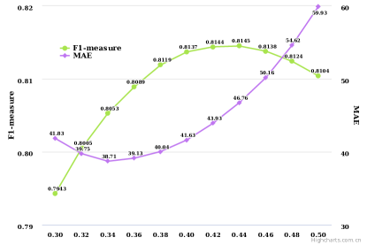
Figure 4: The performance of F1-measure and MAE under different threshold selections.

V-A Trade-off between Localization and Counting Performance

In the experiments, we find that the selection of threshold affects the performance for localization and counting significantly. For further exploring this problem, Fig. 4 shows the F1-measure and the MAE by the way of line chart on the NWPU validation set, where F1-measure and MAE represent the localization and counting performance, respectively. Notably, F1-measure and MAE is calculated under different threshold (in $\{0.30,\;0.32,\;0.34,\;...,\;0.50\}$). From the figure, we find the best F1-measure of 81.45% and MAE of 38.71 locates at 0.44 and 0.32, respectively.

The main reason is that there are more independent areas at low thresholds. For the localization task, the model tends to produce high-confidence prediction to achieve higher F1-measure, which results in missing many objects. Generally, the counting number is less than the GT in crowd scenes. As the threshold decreases, more independent regions are output by the model. Although many False Positives (FP) are included, the counting number is increased, which is closer to the GT in most cases. As a result, the best MAE is under a low-value threshold.

V-B Analysis of DCB’s Location in Encoder

Swin Transformer contains four stages, which have different dimensions. In this section, we analyze where Dilated Convolutional Block (DCB) should be added in the traditional Swin Transformer. To be specific, the four configurations are compared in Table IV: the checkmark means that DCB is added to the corresponding stage. All models are evaluated on the NWPU-Crowd validation set. Each DCB consists of two dilated convolutional layers with the dilatation rate of 2 and 3, respectively.

From the table, when DCB is inserted into Stage 3 and 4, the performance is the best, namely F1-measure of 81.4, Precision of 84.1, and Recall of 79.0. Based on this setting, the performance is reduced when DCB is added to Stage 2 and 1. In fact, the shallow layer focus on learning local structure patterns. Introducing a large-range encoder (such as the proposed DCB) reduces the ability to extract local features of the model.

V-C Design of DCB

TABLE IV: The results (F1-measure/Pre./Rec.) of different Dilated Convolutional Backbones on the NWPU-Crowd validation set. (%)

Stage1	Stage2	Stage3	Stage4	F1-m	Pre.	Rec.
✔	✔	✔	✔	79.2	81.6	76.9
	✔	✔	✔	80.0	83.1	77.2
		✔	✔	81.4	84.1	79.0
			✔	80.8	83.5	78.3

The last section discusses the impact of DCB’s location in Swin Transformer. Besides, the configuration inside DCB will affect the performance of the entire localization model. This section conducts the experiments of different dilatation rates in DCB on the NWPU validation set. Specifically, following the HDC’s idea [60], three groups of dilatation rate settings are designed: $\{2,\;2\}$, $\{2,\;3\}$ and $\{2,\;5\}$. The DCB is inserted into Stage 3 and 4 in Swin Transformer.

TABLE V: The results (F1-measure/Pre./Rec.) of different Dilated Convolutional Blocks on the NWPU-Crowd validation set. (%)

Dilatation Rate	F1-m	Pre.	Rec.
$\{2,\;2\}$	80.1	87.5	73.8
$\{2,\;3\}$	81.4	84.1	79.0
$\{2,\;5\}$	80.2	82.9	77.6

Table V reports the localization results of the aforementioned settings. Notably, the dilatation rate of $\{2,\;3\}$ obtains the best performance, F1-measure of 81.4, Precision of 84.1, and Recall of 79.0. From the results, we find that too large or too small a receptive field will reduce the performance of the model. The former may learn more contextual information so that miss the local structure patterns, which will perform poorly in some clear scenes. The latter loses more large-range features, which causes that the model cannot handle dense and blurred crowd regions. Therefore, this paper selects the DCB with the dilatation rate of $\{2,\;3\}$ to achieve better performance.

VI Conclusion

This paper proposes a joint of transformer and traditional convolutional networks method to tackle dense prediction problem for crowd localization. Notably, in Swin Transformer backbone, two dilated convolutional blocks are inserted in different stages to enlarge the respective field, which effectively prompts the capacity of feature extraction, especially for tiny objects, mutual occlusion, and blurred regions in the crowd scenes. Extensive experiments show the effectiveness of the proposed mechanism and achieve state-of-the-art performance on six mainstream datasets. Besides, this paper further discusses the relationship of performance between localization and counting tasks by some interesting experimental phenomena. In the future, we will focus on exploring the difference in learning parameters between the two tasks.

References

- [1] L. Liu, Z. Qiu, G. Li, S. Liu, W. Ouyang, and L. Lin, “Crowd counting with deep structured scale integration network,” in 2019 IEEE/CVF International Conference on Computer Vision, ICCV 2019, Seoul, Korea (South), October 27 - November 2, 2019, 2019, pp. 1774–1783.
- [2] J. Gao, Y. Yuan, and Q. Wang, “Feature-aware adaptation and density alignment for crowd counting in video surveillance,” IEEE Transactions on Cybernetics, 2020.
- [3] J. Wan, N. S. Kumar, and A. B. Chan, “Fine-grained crowd counting,” IEEE transactions on image processing, vol. 30, pp. 2114–2126, 2021.
- [4] J. Cheng, H. Xiong, Z. Cao, and H. Lu, “Decoupled two-stage crowd counting and beyond,” IEEE Transactions on Image Processing, vol. 30, pp. 2862–2875, 2021.
- [5] J. Wan, Z. Liu, and A. B. Chan, “A generalized loss function for crowd counting and localization,” in Proceedings of the IEEE/CVF Conference on Computer Vision and Pattern Recognition (CVPR), June 2021, pp. 1974–1983.
- [6] A. S. Rao, J. Gubbi, S. Marusic, and M. Palaniswami, “Crowd event detection on optical flow manifolds,” IEEE transactions on cybernetics, vol. 46, no. 7, pp. 1524–1537, 2015.
- [7] Z. Lin, J. Feng, Z. Lu, Y. Li, and D. Jin, “Deepstn+: Context-aware spatial-temporal neural network for crowd flow prediction in metropolis,” in The Thirty-Third AAAI Conference on Artificial Intelligence. AAAI Press, 2019, pp. 1020–1027.
- [8] A. Alahi, K. Goel, V. Ramanathan, A. Robicquet, F. Li, and S. Savarese, “Social LSTM: human trajectory prediction in crowded spaces,” in 2016 IEEE Conference on Computer Vision and Pattern Recognition, CVPR 2016, Las Vegas, NV, USA, June 27-30, 2016. IEEE Computer Society, 2016, pp. 961–971. [Online]. Available: https://doi.org/10.1109/CVPR.2016.110
- [9] Y. Yuan, J. Fang, and Q. Wang, “Online anomaly detection in crowd scenes via structure analysis,” IEEE transactions on cybernetics, vol. 45, no. 3, pp. 548–561, 2014.
- [10] W. Lin, J. Gao, Q. Wang, and X. Li, “Learning to detect anomaly events in crowd scenes from synthetic data,” Neurocomputing, vol. 436, pp. 248–259, 2021.
- [11] X. LI and B. ZHAO, “Video distillation,” SCIENCE CHINA Information Sciences, 2021.
- [12] B. Zhao, H. Li, X. Lu, and X. Li, “Reconstructive sequence-graph network for video summarization,” CoRR, vol. abs/2105.04066, 2021.
- [13] X. Li, M. Chen, F. Nie, and Q. Wang, “A multiview-based parameter free framework for group detection,” in AAAI, 2017.
- [14] X. Li, M. Chen, and Q. Wang, “Quantifying and detecting collective motion in crowd scenes,” IEEE Transactions on Image Processing, vol. 29, pp. 5571–5583, 2020.
- [15] Q. Wang, M. Chen, F. Nie, and X. Li, “Detecting coherent groups in crowd scenes by multiview clustering,” IEEE Trans. Pattern Anal. Mach. Intell., vol. 42, no. 1, pp. 46–58, 2020.
- [16] S. Ren, K. He, R. Girshick, and J. Sun, “Faster r-cnn: Towards real-time object detection with region proposal networks,” in NIPS, 2015, pp. 91–99.
- [17] J. Redmon, S. K. Divvala, R. B. Girshick, and A. Farhadi, “You only look once: Unified, real-time object detection,” in 2016 IEEE Conference on Computer Vision and Pattern Recognition, 2016, pp. 779–788.
- [18] J. Liu, C. Gao, D. Meng, and A. G. Hauptmann, “Decidenet: Counting varying density crowds through attention guided detection and density estimation,” in CVPR, 2018, pp. 5197–5206.
- [19] P. Hu and D. Ramanan, “Finding tiny faces,” in CVPR, 2017, pp. 951–959.
- [20] D. B. Sam, S. V. Peri, A. Kamath, R. V. Babu et al., “Locate, size and count: Accurately resolving people in dense crowds via detection,” PAMI, 2020.
- [21] Y. Wang, J. Hou, X. Hou, and L.-P. Chau, “A self-training approach for point-supervised object detection and counting in crowds,” IEEE Transactions on Image Processing, vol. 30, pp. 2876–2887, 2021.
- [22] J. Gao, T. Han, Y. Yuan, and Q. Wang, “Learning independent instance maps for crowd localization,” CoRR, vol. abs/2012.04164, 2020.
- [23] Z. Liu, Y. Lin, Y. Cao, H. Hu, Y. Wei, Z. Zhang, S. Lin, and B. Guo, “Swin transformer: Hierarchical vision transformer using shifted windows,” arXiv preprint arXiv:2103.14030, 2021.
- [24] T. Lin, P. Dollár, R. B. Girshick, K. He, B. Hariharan, and S. J. Belongie, “Feature pyramid networks for object detection,” in 2017 IEEE Conference on Computer Vision and Pattern Recognition, 2017, pp. 936–944.
- [25] X. Liu, P. H. Tu, J. Rittscher, A. Perera, and N. Krahnstoever, “Detecting and counting people in surveillance applications,” in IEEE Conference on Advanced Video and Signal Based Surveillance, 2005. IEEE, 2005, pp. 306–311.
- [26] M. Andriluka, S. Roth, and B. Schiele, “Pictorial structures revisited: People detection and articulated pose estimation,” in 2009 IEEE conference on computer vision and pattern recognition. IEEE, 2009, pp. 1014–1021.
- [27] P. F. Felzenszwalb and D. P. Huttenlocher, “Pictorial structures for object recognition,” International journal of computer vision, vol. 61, no. 1, pp. 55–79, 2005.
- [28] M. Andriluka, S. Roth, and B. Schiele, “People-tracking-by-detection and people-detection-by-tracking,” in 2008 IEEE Conference on computer vision and pattern recognition. IEEE, 2008, pp. 1–8.
- [29] M. Rodriguez, I. Laptev, J. Sivic, and J.-Y. Audibert, “Density-aware person detection and tracking in crowds,” in 2011 International Conference on Computer Vision. IEEE, 2011, pp. 2423–2430.
- [30] T. Van Oosterhout, S. Bakkes, B. J. Kröse et al., “Head detection in stereo data for people counting and segmentation,” in VISAPP, 2011, pp. 620–625.
- [31] R. Stewart, M. Andriluka, and A. Y. Ng, “End-to-end people detection in crowded scenes,” in CVPR, 2016, pp. 2325–2333.
- [32] P. Sermanet, D. Eigen, X. Zhang, M. Mathieu, R. Fergus, and Y. LeCun, “Overfeat: Integrated recognition, localization and detection using convolutional networks,” arXiv preprint arXiv:1312.6229, 2013.
- [33] Z. Li, X. Tang, J. Han, J. Liu, and R. He, “Pyramidbox++: High performance detector for finding tiny face,” arXiv preprint arXiv:1904.00386, 2019.
- [34] J. Deng, J. Guo, Y. Zhou, J. Yu, I. Kotsia, and S. Zafeiriou, “Retinaface: Single-stage dense face localisation in the wild,” arXiv preprint arXiv:1905.00641, 2019.
- [35] H. Idrees, M. Tayyab, K. Athrey, D. Zhang, S. Al-Maadeed, N. Rajpoot, and M. Shah, “Composition loss for counting, density map estimation and localization in dense crowds,” in ECCV, 2018, pp. 532–546.
- [36] C. Liu, X. Weng, and Y. Mu, “Recurrent attentive zooming for joint crowd counting and precise localization,” in CVPR, 2019, pp. 1217–1226.
- [37] J. Gao, T. Han, Q. Wang, and Y. Yuan, “Domain-adaptive crowd counting via inter-domain features segregation and gaussian-prior reconstruction,” arXiv preprint arXiv:1912.03677, 2019.
- [38] J. Wan and A. Chan, “Modeling noisy annotations for crowd counting,” Advances in Neural Information Processing Systems, vol. 33, 2020.
- [39] Y. Wang, X. Hou, and L.-P. Chau, “Dense point prediction: A simple baseline for crowd counting and localization,” arXiv preprint arXiv:2104.12505, 2021.
- [40] X. Zhou, D. Wang, and P. Krähenbühl, “Objects as points,” arXiv preprint arXiv:1904.07850, 2019.
- [41] D. Liang, W. Xu, Y. Zhu, and Y. Zhou, “Focal inverse distance transform maps for crowd localization and counting in dense crowd,” arXiv preprint arXiv:2102.07925, 2021.
- [42] Q. Wang, J. Gao, W. Lin, and X. Li, “Nwpu-crowd: A large-scale benchmark for crowd counting and localization,” PAMI, 2020.
- [43] S. Abousamra, M. Hoai, D. Samaras, and C. Chen, “Localization in the crowd with topological constraints,” 2021.
- [44] J. Gao, T. Han, Y. Yuan, and Q. Wang, “Learning independent instance maps for crowd localization,” arXiv preprint arXiv:2012.04164, 2020.
- [45] A. Vaswani, N. Shazeer, N. Parmar, J. Uszkoreit, L. Jones, A. N. Gomez, L. Kaiser, and I. Polosukhin, “Attention is all you need,” arXiv preprint arXiv:1706.03762, 2017.
- [46] A. Dosovitskiy, L. Beyer, A. Kolesnikov, D. Weissenborn, X. Zhai, T. Unterthiner, M. Dehghani, M. Minderer, G. Heigold, S. Gelly et al., “An image is worth 16x16 words: Transformers for image recognition at scale,” arXiv preprint arXiv:2010.11929, 2020.
- [47] L. Yuan, Y. Chen, T. Wang, W. Yu, Y. Shi, Z. Jiang, F. E. Tay, J. Feng, and S. Yan, “Tokens-to-token vit: Training vision transformers from scratch on imagenet,” arXiv preprint arXiv:2101.11986, 2021.
- [48] W. Wang, E. Xie, X. Li, D.-P. Fan, K. Song, D. Liang, T. Lu, P. Luo, and L. Shao, “Pyramid vision transformer: A versatile backbone for dense prediction without convolutions,” arXiv preprint arXiv:2102.12122, 2021.
- [49] K. Han, A. Xiao, E. Wu, J. Guo, C. Xu, and Y. Wang, “Transformer in transformer,” arXiv preprint arXiv:2103.00112, 2021.
- [50] D. Liang, X. Chen, W. Xu, Y. Zhou, and X. Bai, “Transcrowd: Weakly-supervised crowd counting with transformer,” arXiv preprint arXiv:2104.09116, 2021.
- [51] G. Sun, Y. Liu, T. Probst, D. Paudel, N. Popovic, and L. Van Gool, “Boosting crowd counting with transformers,” arXiv preprint arXiv:2105.10926, 2021.
- [52] J. Devlin, M.-W. Chang, K. Lee, and K. Toutanova, “Bert: Pre-training of deep bidirectional transformers for language understanding,” arXiv preprint arXiv:1810.04805, 2018.
- [53] T. B. Brown, B. Mann, N. Ryder, M. Subbiah, J. Kaplan, P. Dhariwal, A. Neelakantan, P. Shyam, G. Sastry, A. Askell et al., “Language models are few-shot learners,” arXiv preprint arXiv:2005.14165, 2020.
- [54] N. Carion, F. Massa, G. Synnaeve, N. Usunier, A. Kirillov, and S. Zagoruyko, “End-to-end object detection with transformers,” in European Conference on Computer Vision. Springer, 2020, pp. 213–229.
- [55] L. J. Ba, J. R. Kiros, and G. E. Hinton, “Layer normalization,” CoRR, vol. abs/1607.06450, 2016.
- [56] D. Hendrycks and K. Gimpel, “Gaussian error linear units (gelus),” arXiv preprint arXiv:1606.08415, 2016.
- [57] F. Yu and V. Koltun, “Multi-scale context aggregation by dilated convolutions,” arXiv preprint arXiv:1511.07122, 2015.
- [58] S. Ioffe and C. Szegedy, “Batch normalization: Accelerating deep network training by reducing internal covariate shift,” in International conference on machine learning. PMLR, 2015, pp. 448–456.
- [59] T.-Y. Lin, P. Dollár, R. Girshick, K. He, B. Hariharan, and S. Belongie, “Feature pyramid networks for object detection,” in CVPR, 2017, pp. 2117–2125.
- [60] P. Wang, P. Chen, Y. Yuan, D. Liu, Z. Huang, X. Hou, and G. Cottrell, “Understanding convolution for semantic segmentation,” in 2018 IEEE winter conference on applications of computer vision (WACV). IEEE, 2018, pp. 1451–1460.
- [61] I. Loshchilov and F. Hutter, “Decoupled weight decay regularization,” arXiv preprint arXiv:1711.05101, 2017.
- [62] V. A. Sindagi, R. Yasarla, and V. M. Patel, “Jhu-crowd++: Large-scale crowd counting dataset and a benchmark method,” Technical Report, 2020.
- [63] V. Sindagi, R. Yasarla, and V. Patel, “Pushing the frontiers of unconstrained crowd counting: New dataset and benchmark method,” in Proceedings of the IEEE International Conference on Computer Vision, 2019, pp. 1221–1231.
- [64] Y. Fang, B. Zhan, W. Cai, S. Gao, and B. Hu, “Locality-constrained spatial transformer network for video crowd counting,” in ICME. IEEE, 2019, pp. 814–819.
- [65] Y. Zhang, D. Zhou, S. Chen, S. Gao, and Y. Ma, “Single-image crowd counting via multi-column convolutional neural network,” in CVPR, 2016, pp. 589–597.
- [66] J. Gao, W. Lin, B. Zhao, D. Wang, C. Gao, and J. Wen, “C3 framework: An open-source pytorch code for crowd counting,” arXiv preprint arXiv:1907.02724, 2019.
- [67] C. Xu, D. Liang, Y. Xu, S. Bai, W. Zhan, X. Bai, and M. Tomizuka, “Autoscale: learning to scale for crowd counting,” arXiv preprint arXiv:1912.09632, 2019.