High-resolution chirplet transform: from parameters analysis to parameters combination

Abstract

The standard chirplet transform (CT) with a chirp-modulated Gaussian window provides a valuable tool for analyzing linear chirp signals. The parameters present in the window determine the performance of the CT and play a vital role in high-resolution time-frequency (TF) analysis. In this paper, we give the window shape analysis of the CT and compare it with the extension that employs a rotating Gaussian window by the fractional Fourier transform. The given parameters analysis provides theoretical guidance for developing high-resolution CT. We then propose a multi-resolution chirplet transform (MrCT) by combining multiple CTs with different parameter combinations. These are combined geometrically to obtain an improved TF resolution by overcoming the limitations of any single representation of the CT. By deriving a combined instantaneous frequency equation, we further develop a high-concentration TF post-processing approach to improve the readability of the MrCT. Numerical experiments on simulated and real signals verify the effectiveness of the proposed methods.

I Introduction

Multi-component non-stationary signals are widely observed in many real-world applications, such as seismic [1,2], radar and sonar [3,4], biomedicine [5,6], and mechanical engineering [7,8]. Such signals contain several components with time-varying characteristics and often express complex oscillation content (like fast-varying or closely-spaced instantaneous frequencies (IFs)) [4-6,9]. To capture the useful characteristics of multi-component non-stationary signals as accurately as possible is of great significance for various applications because that can provide insight into the complex structure of the signal, help to understand the data system and predict its future behavior.

Time-frequency (TF) analysis methods [10] provide an effective tool for characterizing multi-component non-stationary signals with time-varying frequency content. In the past decades, the study of reliable TF representations for non-stationary signal analysis has been a hot research topic. The most well-known TF method is the linear TF transforms, such as the short-time Fourier transform (STFT) [11], the continuous wavelet transform (CWT) [12], and the chirplet transform (CT) [13]. In linear TF analysis, the signal is studied via inner products with a pre-assigned basis. The main limitation of this kind of method is that they can not precisely localize a signal in both time and frequency simultaneously because of the effect of the Heisenberg uncertainty principle [5,10]. In order to achieve high TF resolution, the bilinear TF representations, represented by the Wigner-Ville distribution (WVD) [14], are presented. Good TF resolution can be obtained by the WVD but in addressing multi-component or non-linear frequency modulated signals, it suffers from cross-terms (TF artifacts), which renders it unusable for some practical applications [15]. Various smoothed versions of WVD by introducing kernel smoothing are developed to reduce the unwanted inferences, which leads to the Cohen’s class or Affine class [10,16], but the kernel smoothing again blurs the TF distribution.

To increase TF concentration and obtain good TF readability, the post-processing methods of linear TF representations have been widely studied. The reassignment method (RM) [17,18] reallocates the TF coefficients from the original position to the center of gravity of the signal’s energy distribution such that a sharpened TF representation is yielded. As a special case of RM, the synchrosqueezing transform (SST), put forward by Daubechies and Maes in the mid-1990s [19], squeezes the TF coefficients into the instantaneous frequency (IF) trajectory only in the frequency direction, which not only improves the TF concentration but also allows for signal reconstruction [20]. Over the last decade, the SST has received considerable research attentions. It has been extended to different transform frameworks, including the STFT-based SST [21], the synchrosqueezed curvelet transform [22], the synchrosqueezing S-transform [23], the chirplet-based SST [24], etc. It is known that one drawback associated with SST is that it suffers from a low TF resolution when dealing with fast-varying signals [25,26]. To address this drawback, many improvements have been presented involving the demodulated SST [25,27], the high-order SST [26,28], the multiple squeezes transform [24,29], the synchroextracting chirplet transform [30], and the time-reassigned SST [31,32]. The TF post-processing methods introduced above have been increasingly used and adapted in many fields [6,7,23,27,28,31,32]. However, these methods have the intrinsic limitation that they operate on a linear TF representation, associated with a fixed TF resolution given by a global window or wavelet.

In order to improve the TF resolution more essentially, many adaptive TF analysis methods have been proposed. In [33], an adaptive STFT using Gaussian window function with time-varying variance (i.e., window width) dependent on the chirp rate (CR) of the input signal is proposed. A more powerful adaptive STFT is developed in [34,35], where the variance used in the window function is time-frequency-varying because there exist multiple different CRs at the same time instant for multi-component signals. S. Pei et. al [36] also presented an improved version of adaptive STFT with a chirp-modulated Gaussian window. In [37], L. Li et al. proposed the adaptive SST and its second-order extension based on the adaptive STFT with a time-varying window to further enhance the TF concentration. In addition to adaptive STFT-based methods, the adaptive wavelet transform (AWT) [38] is developed by adjusting the wavelet parameter. The bionic wavelet transform, proposed by Yao and Zhang [39], introduces an extra parameter to adaptively adjust the TF resolution not only by the frequency but also by the instantaneous amplitude and its first-order differential. The energy concentration of the S-transform has been addressed in [40,41] by optimizing the width of the window function used. Moreover, the adaptive WVD has been developed by designing different types of filters in the ambiguity domain. L. Stanković [42] proposed L-class WVD; Boashash and O’Shea [43] proposed the polynomial WVD for analyzing polynomial phase signals; Katkovnik [44] presented the local polynomial WVD; Jones and Baraniuk [45] proposed the adaptive optimal kernel TF distribution by introducing a signal-dependent radially Gaussian kernel that adapts over time. Since 2013, Khan et al. conducted a series of research in developing adaptive WVD, mainly involving the adaptive fractional spectrogram [46], the adaptive directional TF distribution [47], the locally optimized adaptive directional TF distribution [48]. Despite the high TF resolution, the adaptive TF representations, especially the adaptive non-linear TF analysis, generally have high computational complexity, and determining the matching parameters remains challenging [48,49].

Other high-resolution methods are based on the combination of multiple spectrograms or wavelet transforms [5,50,51]. The combined methods compute the geometric mean of multiple estimates with short and long windows or a set of wavelets, and have been shown to result in good joint TF resolution for signals consisting of mixtures of tones and pulses [5,50]. Such combinations of conventional spectrograms or wavelet transforms do not work well, however, for signals containing mixtures of chirp-like signals; moreover, how to improve the TF readability of the combinated transformations is an important problem to be solved.

The chirplet transform (CT), proposed by Mann and Haykin [13], Milhovilovic and Bracewell [52] almost at the same time, is a popular TF analysis method for characterizing chirp-like signals, and it has been widely applied in different areas such as radar [53,54], biomedicine [55], and mechanical engineering [56,57]. This method uses an extra CR parameter than STFT (i.e., using a chirp-modulated window function, also termed chirp basis) to characterize linear frequency variation. When the parameter equals to the chirp rate of a signal and the input window length is matching, the CT will generate a highly concentrated TF representation. This fact leads to the development of many adaptive CTs, such as the self-tuning CT [58], the general linear CT [56], the synchro-compensating CT [59], and the double-adaptive CT [54]. The adaptability of such methods is achieved by modifying the window width or/and CR parameter depending on the instantaneous signal’s nature. However, these adaptive CTs are also confronted with the challenges of high computational complexity and parameter matching, as most adaptive TF analysis methods do. To better deal with the signals with non-linear IFs, the CT has been extended to general parameterized TF transforms, which involve the warblet transform [60,61], the polynomial CT [62], the spline-kernelled CT [63], and the scaling-basis CT [57]. Besides, the CT also can be seen as a three-dimensional analysis method as it represents a signal in the joint time-frequency-CR domain when considering the CR parameter as a variable [13,53]. In this sense, the CT enables separating the intersected signals with cross-over IFs by utilizing the CR information. The theoretical analysis and high-concentration representation of three-dimensional CT are recently introduced in [64-66].

Differing from the extensions of CT above, here we introduce a high-resolution analysis approach by combining multiple CTs with different window widths and CR values, which can help to achieve a high-resolution TF representation by overcoming limitations of any single representation of the CT. In this paper, we first theoretically analyze the effect of variance and CR parameters on the TF resolution of CT and prove that a narrow window limits the matching capacity of chirp basis. We compare the CT with its extension that employs a rotating Gaussian window by the fractional Fourier transform [67,68]. By comparison, we conclude that the parameters of rotation-window CT have a clearer geometric meaning than that of the standard CT, but this rotation extension is actually the CT with a special parameter combination and thus can not localize a signal in both time and frequency precisely. To obtain a high-resolution TF representation, we propose a multi-resolution CT (MrCT) by computing the geometric mean of multiple CTs with different parameter combinations, which localizes the signal in both time and frequency better than it is possible with any single CT. Finally, we develop a TF post-processing method to improve the readability of MrCT based on a combined IF equation.

The remainder of the paper is organized as follows. In Section II, the parameter analysis of the standard CT and rotation-window CT is presented. In Section III, we describe the details of the proposed MrCT method. The post-processing TF method, named multi-resolution synchroextracting chirplet transform, is presented in Section IV. Experimental results and comparative studies are introduced in Section V. Finally, the conclusions are drawn in Section VI.

II Window shape analysis of CT and its rotation-window extension

The following sections provide parameters analysis of CT and compare it with a rotation-window CT.

II-A Signal model

In this paper we consider the amplitude-modulation and frequency-modulation (AM-FM) model to describe the time-varying features of multi-component non-stationary signals, which is given by

$$f(t)=\sum_{k=1}^{K}f_{k}(t)=\sum_{k=1}^{K}A_{k}(t)\mathrm{e}^{j\phi_{k}(t)},$$ (1)

where $K$ is a positive integer representing the number of AM-FM components, $\sqrt{-1}=j$ denotes the imaginary unit, $A_{k}(t)>0$ and $\phi_{k}(t)$ are the instantaneous amplitude and instantaneous phase of the $k$-th component (or mode), respectively. The first and the second derivatives of the phase, i.e., $\phi^{\prime}_{k}(t)$, $\phi^{\prime\prime}_{k}(t)$, are referred to as the instantaneous frequency (IF) and the chirp rate (CR) of the $k$-th component. To model multi-component non-stationary signals as (1) is important to extract information hidden in $f(t)$, and this representation has been used in many applications including seismic wave analysis, medical data analysis, mechanical vibration diagnosis and speech recognition, see for example [20,38].

The Fourier transform of a given signal $f(t)\in L^{1}(\mathbb{R})$, i.e. its correlation with a sinusoidal wave $\mathrm{e}^{j\omega t}$, is defined as

$$\hat{f}(\omega)=\int_{-\infty}^{+\infty}f(t)\mathrm{e}^{-j\omega t}\mathrm{d}t.$$

II-B Window shape analysis of CT

The chirplet transform (CT) [13,52] generalizes the STFT by using an extra CR parameter and its definition is given by

$$\begin{split}C_{f}^{h_{\beta}}(t,\omega)=\int_{-\infty}^{+\infty}f(\mu)g^{*}(t-\mu)\mathrm{e}^{-j\frac{\beta}{2}(\mu-t)^{2}}\mathrm{e}^{-j\omega(\mu-t)}\mathrm{d}\mu,\end{split}$$ (2)

where $\beta$ is the CR parameter/variable, $g(t)$ is a window function in the Schwartz class, superscript $*$ denotes the complex conjugate, and $h_{\beta}(t)=g(t)\mathrm{e}^{j\frac{\beta}{2}t^{2}}$ called the chirp-modulated window. If $\beta=0$, then the CT reduces to the STFT. Importantly, the squared modulus of CT can be interpreted as a smoothed WVD, resulting from the smoothing of the WVD of the signal by the WVD of the chirp-modulated window, as presented in Lemma 1.

Lemma 1.

For a signal $f(t)$, its squared modulus of the CT can be equivalently expressed as

$$|C_{f}^{h_{\beta}}(t,\omega)|^{2}=\frac{1}{2\pi}W_{f}\ast\ast W_{h_{\beta}}(t,\omega),$$ (3)

where $\ast\ast$ denotes the 2D convolution operator, and $W_{f}(t,\omega)$ and $W_{h_{\beta}}(t,\omega)$ are the WVDs of $f(t)$ and $h_{\beta}(t)$ respectively defined as

$$W_{f}(t,\omega) =\int_{-\infty}^{+\infty}f(t+\frac{\tau}{2})f^{*}(t-\frac{\tau}{2})\mathrm{e}^{-j\omega\tau}\mathrm{d}\tau,$$ (4)

$$W_{h_{\beta}}(t,\omega) =\int_{-\infty}^{+\infty}h_{\beta}(t+\frac{\tau}{2})h_{\beta}^{*}(t-\frac{\tau}{2})\mathrm{e}^{-j\omega\tau}\mathrm{d}\tau.$$ (5)

The proof of Lemma 1 is similar to the result in [16,18] for the spectrogram.

From Lemma 1, we can know that the shape of the window, as a TF filter or kernel, is critical because it determines the energy distribution of the CT in multi-component non-stationary signal analysis. A matching one with the TF feature of an observed signal can help for obtaining a high-resolution TF representation [54,56,58,59].

To further analyze the effect of chirp-based window on CT, we consider a concrete window, i.e., the Gaussian window $g(t)={(\sqrt{2\pi}\sigma)}^{-\frac{1}{2}}\mathrm{e}^{-\frac{t^{2}}{2\sigma^{2}}}$ ($\sigma>0$ is the variance of the window), as this function leads to the optimal TF resolution and based on it the analytic expression of some TF transformations is easy to compute. Denote the chirp-based Gaussian window as

$$\begin{split}h_{\sigma,\beta}(t)=g(t)\mathrm{e}^{j\frac{\beta}{2}t^{2}}={(\sqrt{2\pi}\sigma)}^{-\frac{1}{2}}\mathrm{e}^{-\frac{t^{2}}{2\sigma^{2}}}\mathrm{e}^{j\frac{\beta}{2}t^{2}},\end{split}$$ (6)

then the corresponding CT can be expressed by

$$\begin{split}&C_{f}^{h_{\sigma,\beta}}(t,\omega)=\\ &(\sqrt{2\pi}\sigma)^{-\frac{1}{2}}\int_{-\infty}^{+\infty}f(\mu)\mathrm{e}^{-\frac{(t-\mu)^{2}}{2\sigma^{2}}}\mathrm{e}^{-j\frac{\beta}{2}(\mu-t)^{2}}\mathrm{e}^{-j\omega(\mu-t)}\mathrm{d}\mu.\end{split}$$ (7)

The WVD of this window $h_{\sigma,\beta}(t)$ is calculated as

$$\begin{split}W_{h_{\sigma,\beta}}(t,\omega)&=\int_{-\infty}^{+\infty}h_{\sigma,\beta}(t+\frac{\tau}{2})h_{\sigma,\beta}^{*}(t-\frac{\tau}{2})\mathrm{e}^{-j\omega\tau}\mathrm{d}\tau\\ &=\sqrt{2}\mathrm{e}^{-\frac{t^{2}}{\sigma^{2}}-\sigma^{2}(\omega-\beta t)^{2}}.\end{split}$$ (8)

Obviously, the shape of $W_{h_{\sigma,\beta}}(t,\omega)$ is an oblique ellipse centered at the origin in the TF plane (see Fig. 1), and affected by two parameters, i.e., $\beta$ and $\sigma$. Maybe, the parameter $\beta$ determines the direction of the ellipse axis, and the parameter $\sigma$ determines the size of the ellipse. To make this issue clear, let us consider a level curve of $W_{h_{\sigma,\beta}}(t,\omega)$, which is given by

$$\begin{split}\frac{t^{2}}{\sigma^{2}}+\sigma^{2}(\omega-\beta t)^{2}=C,\end{split}$$ (9)

where $C$ is a positive constant (i.e., percentage of the maximum energy).

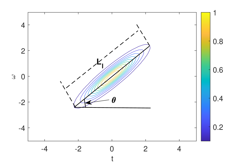
Figure 1: Plot of $W_{h_{\sigma,\beta}}(t,\omega)$ when $\sigma=1.5$ and $\beta=1$.

Clearly, the shape of (9) becomes a circle when $\beta=0$ and $\sigma=1$. Except this special case, the following theorem explains the influence of the parameters $\sigma$ and $\beta$ on the shape of ellipse (9).

Theorem 1.

For ellipse (9), the length of the long axis is that

$$L_{l}=C({A\sigma^{2}}+\frac{2}{\sigma^{2}}+{\sqrt{A^{2}\sigma^{4}+4\beta^{2}}}),$$ (10)

where $A=1+\beta^{2}-\frac{1}{\sigma^{4}}$, and the angle $\theta$ ($\theta\in(-\frac{\pi}{2},\frac{\pi}{2}]$) between $t$-axis and the long axis (see Fig. 1) satisfies

$$\lim_{\sigma\rightarrow+\infty}\tan\theta=\beta,$$ (11)

$$|\tan\theta|\geq\sqrt{\frac{1}{\sigma^{4}}-1}~{}~{}\text{for}~{}~{}0<\sigma<1.$$ (12)

Proof.

See the Supplementary Materials-I. ∎

Theorem 1 throws up some interesting results. On the one hand, the length $L_{l}$ increases with the value of $\beta$ increasing, and also exhibiting an increase with the decrease in value of $\sigma$, which may lead the CT to generate a bad TF result when dealing with strong modulation signals because a large $\beta$ and small $\sigma$ are required to match its fast-varying feature. On the other hand, from the proof (please refer to equation (49) in the Supplementary Materials), we can know that there does not exist a correspondence relationship that $\tan\theta=\beta$ between the rotation angle $\theta$ and parameter $\beta$. But a large value of $\sigma$ is more advisable for CT because based on it the major axis of $W_{h_{\sigma,\beta}}(t,\omega)$ can rotate along any direction to approach that $\tan\theta=\beta$. Moreover, relation (12) shows that $|\tan\theta|$ is bounded and it can not be taken as a sufficiently small value when the input variance is small (e.g., $\sigma\leq 0.1$), which limits the slope range of $W_{h_{\sigma,\beta}}(t,\omega)$, leading to inaccurate match in dealing with short signal segments containing smaller CR values.

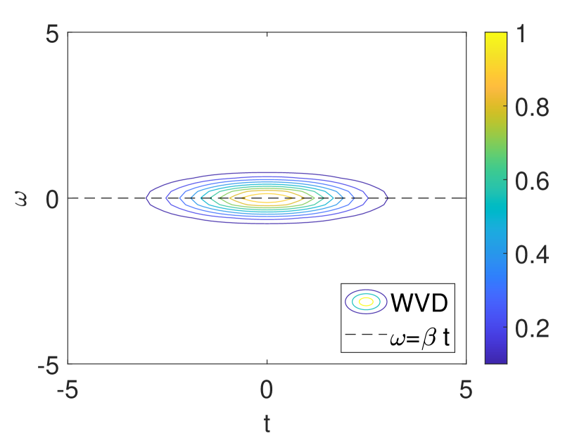
(a)

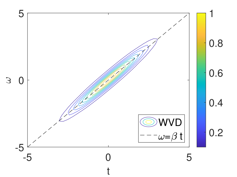
(b)

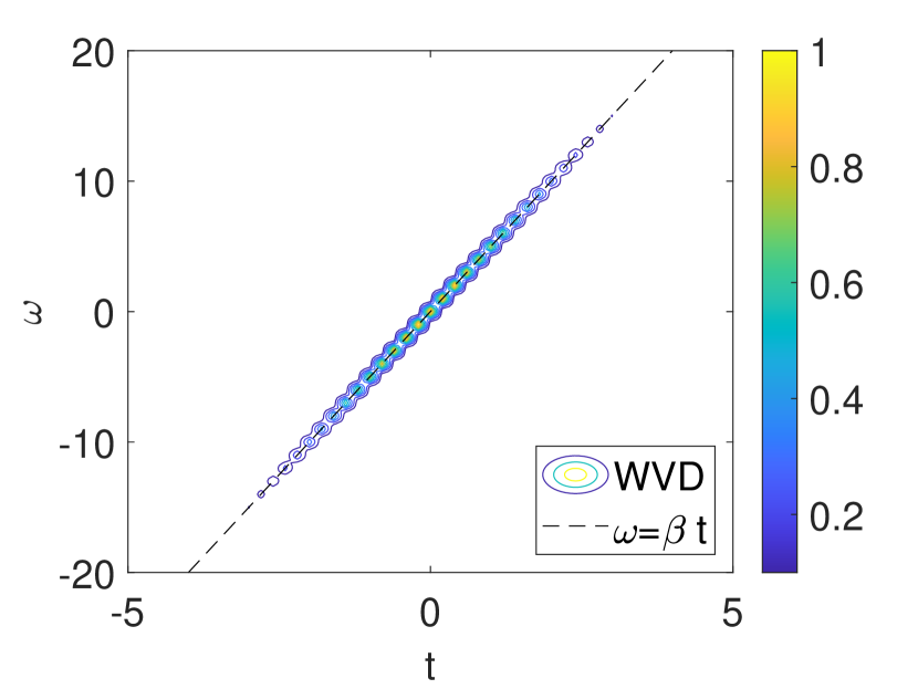
(c)

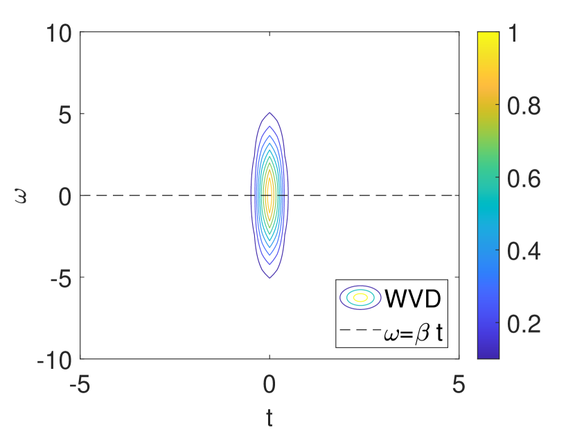
(d)

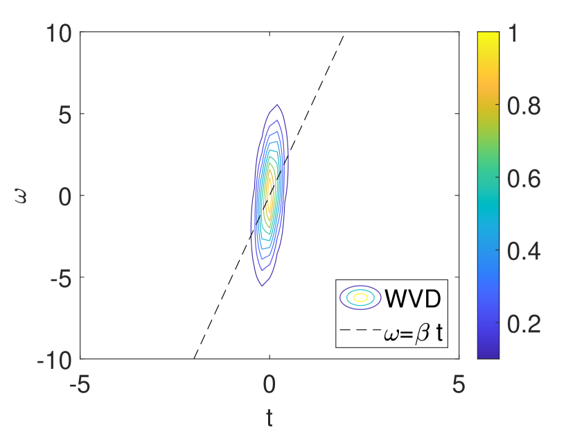
(e)

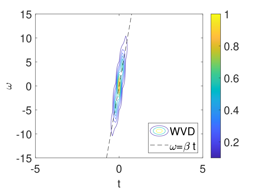
(f)

Figure 2: The WVDs of $h_{\sigma,\beta}(t)$ using various values of $\sigma$ and $\beta$. (a) The WVD with $\sigma=2$ and $\beta=0$, (b) the WVD with $\sigma=2$ and $\beta=1$, (c) the WVD with $\sigma=2$ and $\beta=5$, (d) the WVD with $\sigma=0.3$ and $\beta=0$, (e) the WVD with $\sigma=0.3$ and $\beta=5$, (f) the WVD with $\sigma=0.3$ and $\beta=20$.

Fig. 2 shows the WVDs of the chirp-based Gaussian window using various values of $\beta$ and $\sigma$. The first row in Fig. 2 is the results corresponding to a large variance (i.e., $\sigma=2$) over different values of $\beta$ ($\beta=0$, $\beta=1$, $\beta=5$). It can be seen from the results that the length of the major axis increases with the increasing of $\beta$, and the rotation angle $\theta$ approximately satisfies the relationship that $\tan\theta=\beta$. While using a small $\sigma$ (e.g., $\sigma=0.3$), the length of the major axis also increases with the increasing of $\beta$, but the range of rotation angle $\theta$ is limited in a neighborhood of $\frac{\pi}{2}$ (see Fig. 2(d-f)).

To solve the existing problem of the standard CT, we will discuss the performance of a rotation-window CT in the following setion.

II-C CT with rotation window

In order to obtain a more canonical TF filter, i.e., parameters $\sigma$ and $\beta$ have a clear role in determining the shape of $W_{h_{\sigma,\beta}}(t,\omega)$, we use the fractional Fourier transform (FrFT) [67,68] to rotate Gaussian window $g(t)$ with parameter $\beta$, which is given by

$$\begin{split}\tilde{h}_{\sigma,\beta}(t)=\left(\sqrt{2\pi}\sqrt{\frac{1+\sigma^{2}\beta^{2}}{\sigma(1+\beta^{2})}}\right)^{-\frac{1}{2}}\mathrm{e}^{-\frac{\sigma(1+\beta^{2})}{2(1+\sigma^{2}\beta^{2})}t^{2}}\mathrm{e}^{j\frac{\beta(1-\sigma^{2})}{2(1+\sigma^{2}\beta^{2})}t^{2}}.\end{split}$$ (13)

Using this rotation window, the corresponding CT, named rotation-window CT, is that

$$\begin{split}{C}_{f}^{\tilde{h}_{\sigma,\beta}}(t,\omega)=\int_{-\infty}^{+\infty}f(\mu)\tilde{h}_{\sigma,\beta}(t-\mu)\mathrm{e}^{-j\omega(\mu-t)}\mathrm{d}\mu.\end{split}$$ (14)

Based on Lemma 1, the squared modulus of ${C}_{f}^{\tilde{h}_{\sigma,\beta}}(t,\omega)$ can be expressed as

$$|{C}_{f}^{\tilde{h}_{\sigma,\beta}}(t,\omega)|^{2}=\frac{1}{2\pi}W_{f}\ast\ast W_{\tilde{h}_{\sigma,\beta}}(t,\omega),$$ (15)

where $W_{\tilde{h}_{\sigma,\beta}}$ is the WVD of $\tilde{h}_{\sigma,\beta}(t)$ as follows:

$$\begin{split}W_{\tilde{h}_{\sigma,\beta}}(t,\omega)=\sqrt{2}\mathrm{e}^{-\frac{t^{2}}{\hat{\sigma}^{2}}-\hat{\sigma}^{2}(\omega-\hat{\beta}t)^{2}},\end{split}$$ (16)

with $\hat{\sigma}^{2}=\frac{1+\sigma^{2}\beta^{2}}{\sigma(1+\beta^{2})}$, $\hat{\beta}=\frac{\beta(1-\sigma^{2})}{1+\sigma^{2}\beta^{2}}$.

To discuss parameters $\sigma$ and $\beta$ are how they affect the shape of $W_{\tilde{h}_{\sigma,\beta}}(t,\omega)$, we also consider a level curve of $W_{\tilde{h}_{\sigma,\beta}}$, which is

$$\begin{split}\frac{t^{2}}{\hat{\sigma}^{2}}+\hat{\sigma}^{2}(\omega-\hat{\beta}t)^{2}=C,\end{split}$$ (17)

where $C$ is a positive constant. The follwing theorem shows the determination of the shape of ellipse (17) by parameters $\sigma$ and $\beta$.

Theorem 2.

For ellipse (17), the length $L_{l}$ of the long axis is that

$$L_{l}=\begin{cases}\frac{2C}{\sigma},&\text{if}~{}\sigma<1,\\ 2\sigma C,&\text{if}~{}\sigma\geq 1.\end{cases}$$ (18)

The angle $\theta$ ($\theta\in(-\frac{\pi}{2},\frac{\pi}{2}]$) between $t$-axis and the long axis satisfies

$$\tan\theta=\begin{cases}\beta,&\text{if}~{}~{}0<\sigma<1,\\ -\frac{1}{\beta},&\text{if}~{}\sigma>1,\beta\neq 0,\\ +\infty,&\text{if}~{}\sigma>1,\beta=0.\end{cases}$$ (19)

Proof.

See the Supplementary Materials-II. ∎

For the rotation window $\tilde{h}_{\sigma,\beta}(t)$, Theorem 2 proves that the parameter $\sigma$ determines the size of the WVD of $\tilde{h}_{\sigma,\beta}(t)$, and the parameter $\beta$ determines its inclined direction. This property makes the role of $\beta$ and $\sigma$ more clear and is helpful for parameter setting. Further explanation is given from numerical experiments, which are presented in Fig. 3. From the results, we can see that the size of the WVDs is unchangeable when fixing the value of $\sigma$. Moreover, when using different values of $\beta$, the rotation of the WVD of $\tilde{h}_{\sigma,\beta}(t)$ satisfies the relation (19) given in Theorem 2.

(a)

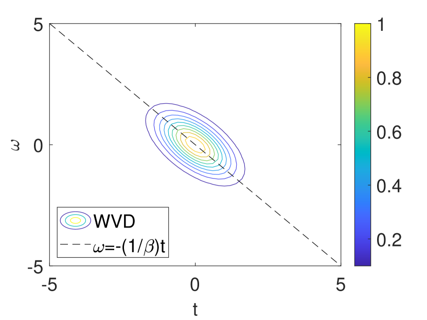
(b)

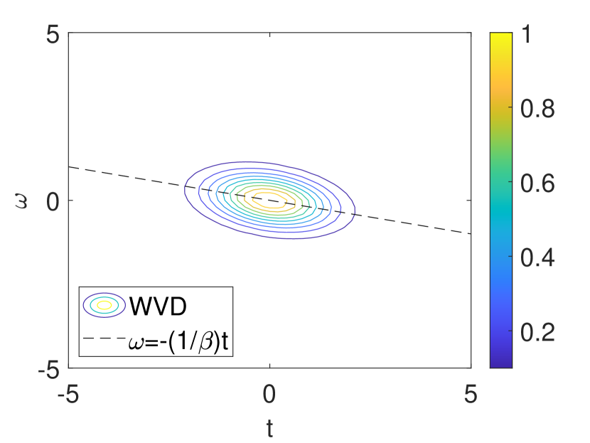
(c)

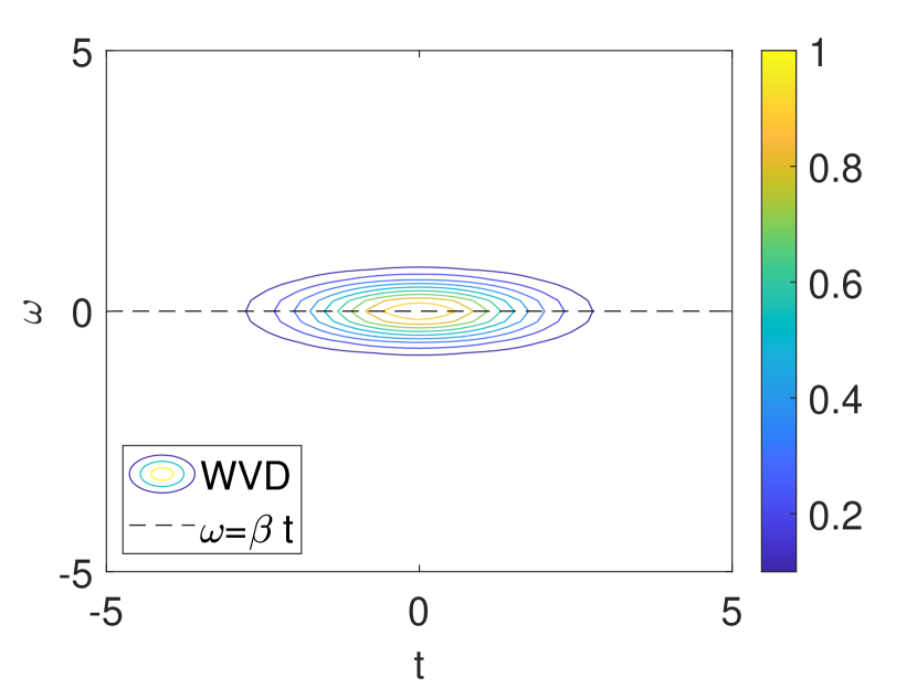
(d)

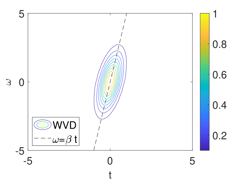
(e)

(f)

Figure 3: The WVDs of $\tilde{h}_{\sigma,\beta}(t)$ using various values of $\sigma$ and $\beta$. (a) The WVD with $\sigma=2$ and $\beta=0$, (b) the WVD with $\sigma=2$ and $\beta=1$, (c) the WVD with $\sigma=2$ and $\beta=5$, (d) the WVD with $\sigma=0.3$ and $\beta=0$, (e) the WVD with $\sigma=0.3$ and $\beta=5$, (f) the WVD with $\sigma=0.3$ and $\beta=20$.

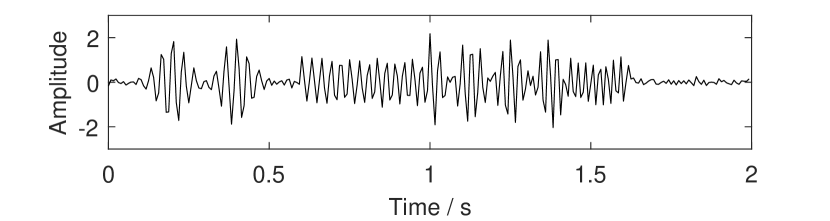
(a)

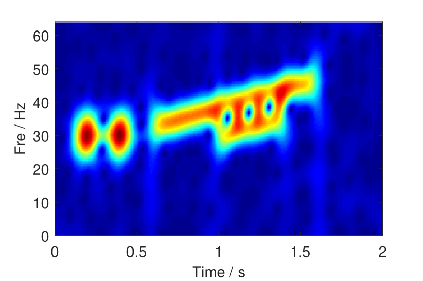
(b)

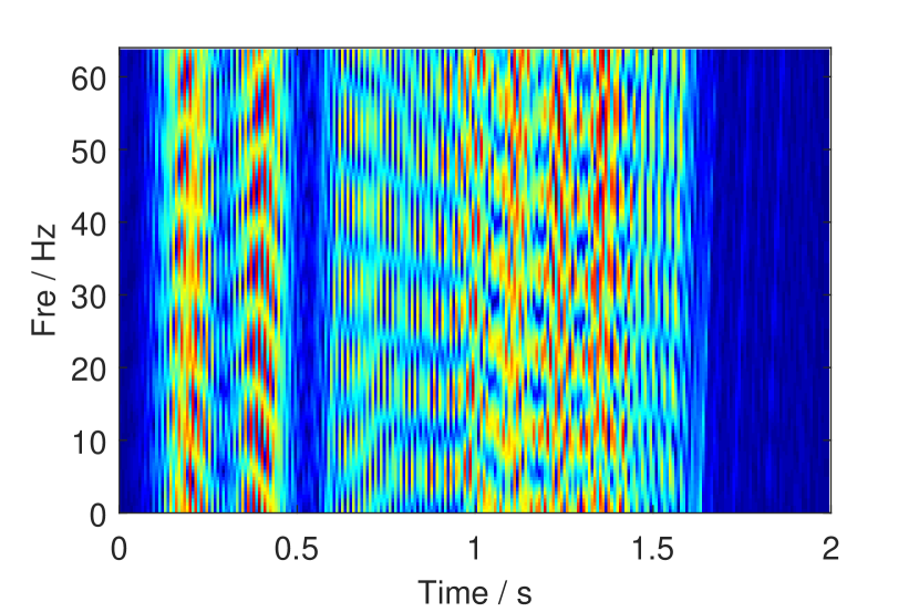
(c)

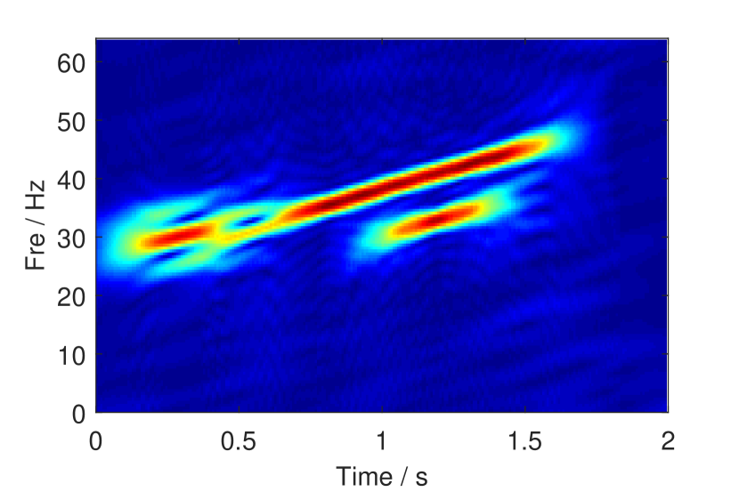
(d)

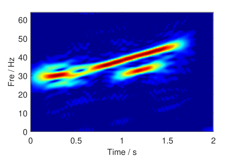
(e)

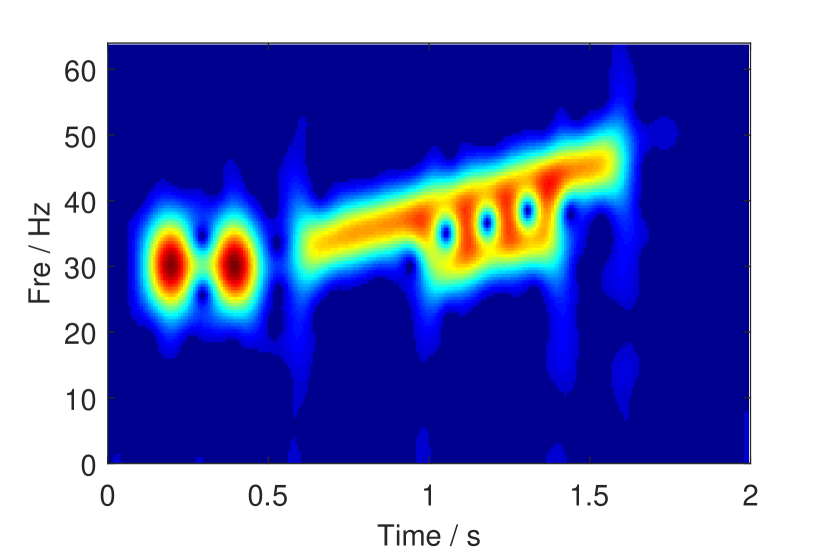
(f)

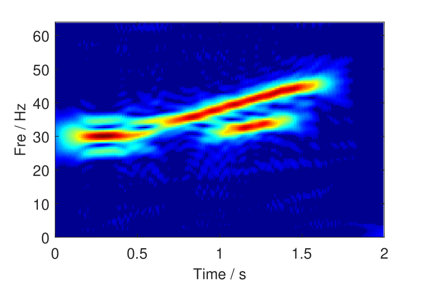
(g)

Figure 4: Evaluation of TF resolution on a known signal structure. (a) Waveform of the test signal, (b) CT with $\sigma=0.1$ and $\beta=7$, (c) CT with $\sigma=0.1$ and $\beta=1000$, (d) CT with $\sigma=0.3$ and $\beta=7$, (e) the rotation-window CT with $\sigma=0.1$ and $\beta=7$, (f) the rotation-window CT with $\sigma=0.1$ and $\beta=1000$, (g) the rotation-window CT with $\sigma=0.3$ and $\beta=7$.

II-D Comparison

The section above mainly discusses the effect of the chirp-based Gaussian window and the rotating Gaussian window on the CT from theory, which provides important theoretical guidance for CT to choose suitable parameters so as to obtain a high-resolution TF representation. In the following, we test the performance of CT and rotation-window CT by an example. The waveform of the test signal is illustrated in Fig. 4(a), which contains two chirp signals (CR$=$7) and two impulse signals. We compute the TF representations of this test signal using CT and rotation-window CT with different parameters (see Fig. 4(b-g)). From the results, we can see that the CT can fully separate the two impulse signals when employing a smaller value of $\sigma$, but a small one results in a poor frequency resolution such that the TF mixing of chirp components occurs (see Fig. 4(b)). A relatively large $\sigma$ following with good CR estimation can resolve the two chirps, and yet obscures the TF information of the two impulses (see Fig. 4(d)). Moreover, using a large $\beta$ to match the fast-varying feature of impulse signals degrades the TF performance of the CT, as presented in Fig. 4(c). By contrast, it follows that the rotation-window CT provides a better time resolution when using a small $\sigma$ and a large $\beta$ (see Fig. 4(f)), and can separate the two chirps even with a small $\sigma$ (see Fig. 4(e)). In fact, an advantage of the rotation-window CT over the standard CT is that the parameters in the window become relative, forming effective combinations such that the window shape can rotate along any direction in the TF plane only by adjusting the parameter $\beta$.

Nevertheless, the rotation-window CT is actually the standard CT with a special parameter combination (i.e., $\hat{\sigma}$ and $\hat{\beta}$), thus it is still limited by the Heisenberg uncertainty principle and can not localize precisely a signal in both time and frequency. As presented in Fig. 4, the window of these two methods matches the pulse (chirp) components well but smears the chirp (pulse) components. This illustrates the fundamental tradeoff of the CT: it is difficult to get both good time and good frequency resolution using a single fixed window.

III Multi-resolution chirplet transform

To overcome the TF resolution problem of the CT, more effective possibilities should be considered. The following section utilizes a combination of multiple CTs with different parameter combinations to improve the TF resolution of the CT, as it can localize the signal in both time and frequency better than it is possible with any single CT. Moreover, the combined one can reduce the computational complexity of adaptive CTs in which the window function is adjusted at every TF location.

III-A Multi-resolution chirplet transform

Let us consider a two-component non-stationary signal including an impulse signal and a chirp signal, which is given by

$$\begin{split}&f(t)=f_{1}(t)+f_{2}(t),\\ &f_{1}(t)=A_{1}\delta(t-t_{0}),~{}f_{2}(t)=A_{2}(t)\mathrm{e}^{j(at+\frac{b}{2}t^{2})},\end{split}$$ (20)

where $A_{1}>0$, $A_{2}(t)\geq 0$, $a,b\in\mathbb{R}$, and $\delta(\cdot)$ is the Dirac delta function.

Assuming that around $\mu=t$ the amplitude $A_{2}(t)$ is slowly varying and can be well approximated by $A_{2}(t+\mu)\approx A_{2}(t)$, then the CT of signal (20) under the Gaussian window $g(t)={(\sqrt{2\pi}\sigma)}^{-1}\mathrm{e}^{-\frac{t^{2}}{2\sigma^{2}}}$ is computed as

$$C_{f}^{h_{\sigma,\beta}}(t,\omega)=\int_{-\infty}^{+\infty}f(\mu)g^{*}(t-\mu)\mathrm{e}^{-j\frac{\beta}{2}(\mu-t)^{2}}\mathrm{e}^{-j\omega(\mu-t)}\mathrm{d}\mu$$

$$={(\sqrt{2\pi}\sigma)}^{-1}\int_{-\infty}^{+\infty}f_{1}(t+\mu)\mathrm{e}^{-\frac{\mu^{2}}{2\sigma^{2}}}\mathrm{e}^{-j\frac{\beta}{2}\mu^{2}}\mathrm{e}^{-j\omega\mu}\mathrm{d}\mu$$

$$+{(\sqrt{2\pi}\sigma)}^{-1}\int_{-\infty}^{+\infty}f_{2}(t+\mu)\mathrm{e}^{-\frac{\mu^{2}}{2\sigma^{2}}}\mathrm{e}^{-j\frac{\beta}{2}\mu^{2}}\mathrm{e}^{-j\omega\mu}\mathrm{d}\mu$$

$$={(\sqrt{2\pi}\sigma)}^{-1}(A_{1}\mathrm{e}^{-\frac{(t_{0}-t)^{2}}{2\sigma^{2}}}\mathrm{e}^{-j\frac{\beta}{2}(t_{0}-t)^{2}}\mathrm{e}^{-j\omega(t_{0}-t)}+$$

$$\mathrm{e}^{j(at+\frac{b}{2}t^{2})}\int_{-\infty}^{+\infty}A_{2}(t+\mu)\mathrm{e}^{-\frac{\mu^{2}}{2\sigma^{2}}}\mathrm{e}^{-j\frac{(\beta-b)}{2}\mu^{2}}\mathrm{e}^{-j(\omega-a-bt)\mu}\mathrm{d}\mu)$$

$$\approx{(\sqrt{2\pi}\sigma)}^{-1}A_{1}\mathrm{e}^{-\frac{(t_{0}-t)^{2}}{2\sigma^{2}}}\mathrm{e}^{-j\frac{\beta}{2}(t_{0}-t)^{2}}\mathrm{e}^{-j\omega(t_{0}-t)}$$

$$+{(\sqrt{2\pi}\sigma)}^{-1}f_{2}(t)\int_{-\infty}^{+\infty}\mathrm{e}^{-\frac{\mu^{2}}{2\sigma^{2}}}\mathrm{e}^{-j\frac{(\beta-b)}{2}\mu^{2}}\mathrm{e}^{-j(\omega-a-bt)\mu}\mathrm{d}\mu$$

$$\xlongequal[]{\beta=b}{(\sqrt{2\pi}\sigma)}^{-1}A_{1}\mathrm{e}^{-\frac{(t_{0}-t)^{2}}{2\sigma^{2}}}\mathrm{e}^{-j\frac{b}{2}(t_{0}-t)^{2}}\mathrm{e}^{-j\omega(t_{0}-t)}$$

$$+f_{2}(t)\mathrm{e}^{-\frac{\sigma^{2}}{2}(\omega-a-bt)^{2}}.$$ (21)

If $f_{1}(t)$ and $f_{2}(t)$ are further separable, e.g., $A_{2}(t)\approx 0$ when $t\in[t_{0}-\sigma,t_{0}+\sigma]$, then the modulus of CT can be expressed as

$$|C_{f}^{h_{\sigma,b}}(t,\omega)|$$

$$\approx{(\sqrt{2\pi}\sigma)}^{-1}A_{1}\mathrm{e}^{-\frac{1}{2\sigma^{2}}(t_{0}-t)^{2}}+A_{2}(t)\mathrm{e}^{-\frac{\sigma^{2}}{2}(\omega-a-bt)^{2}}.$$ (22)

From (22), we can know that high time-resolution can be achieved for $f_{1}(t)$ with a small value of $\sigma$, but that causes a degradation of frequency resolution. Conversely, a large $\sigma$ increases frequency resolution for $f_{2}(t)$ but at the expense of temporal resolution of the CT of $f_{1}(t)$ (see Fig. 4(b,d) for numerical illustration).

To overcome this problem, let us consider the product of two CTs with different parameters $\sigma_{1}$ and $\sigma_{2}$, which is calculated as

$$|C_{f}^{h_{\sigma_{1},b}}(t,\omega)\times C_{f}^{h_{\sigma_{2},b}}(t,\omega)|\approx\frac{1}{2\pi\sigma_{1}\sigma_{2}}A_{1}^{2}\mathrm{e}^{-\frac{\sigma_{1}^{2}+\sigma_{2}^{2}}{2\sigma_{1}^{2}\sigma_{2}^{2}}(t_{0}-t)^{2}}$$

$$+A_{2}(t)^{2}\mathrm{e}^{-\frac{\sigma_{1}^{2}+\sigma_{2}^{2}}{2}(\omega-a-bt)^{2}}.$$ (23)

Comparing (22) with (23), we find that the product has better time resolution for $f_{1}(t)$ and increased frequency resolution for $f_{2}(t)$ (here we can suppose $\sigma$ and $\sigma_{1}$ (or $\sigma$ and $\sigma_{2}$) take the same value). To make this point more clear, we give the combined CT of the test signal (see Fig. 4(a)) in Fig. 5(a). Obviously, the combined result achieves a sharper TF representation than that by the single CT with $\sigma=0.1$ or $\sigma=0.3$, as presented in Fig. 5(a) and Fig. 4(b,d).

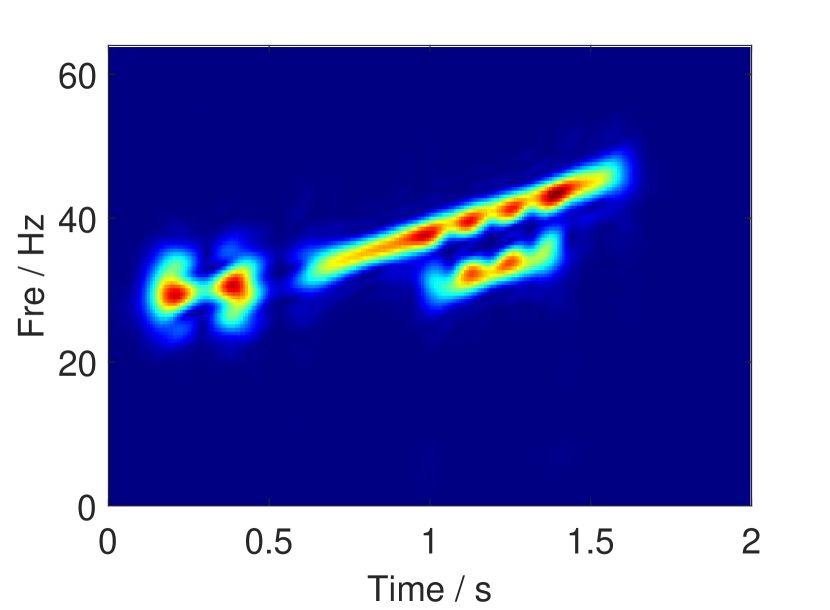
(a)

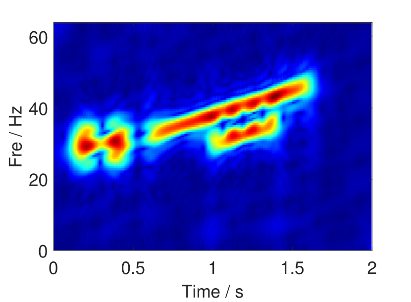
(b)

Figure 5: The results of the combined CT with $\sigma=0.1$ and $\sigma=0.3$ (here $\beta=7$). (a) The product of the two CTs, (b) the geometric mean of the two CTs.

Unlike the adaptive CTs [56,59], the combined CT only uses two parameters $\sigma_{1}$ and $\sigma_{2}$ to yield a high-resolution result, thus it reduces the computational complexity effectively. Meanwhile, it is worth pointing out that, when computing the product of multiple CTs to increase TF resolution, one existing problem is that the magnitude of the combined TF representation may become increasingly polarized with the increase of the number of product-times, i.e., a small TF energy becomes smaller and smaller, and a large one is getting bigger and bigger. Therefore it is undesirable to multiply too many CTs for the combined CT. An effective way to solve the magnitude problem is to compute its geometric mean [5,50,51]. However, the mean step inevitably reduces time and frequency resolution of the TF representation (see Fig. 5(b)). Nevertheless, we can derive the following conclusion based on (22) and (23), which shows the superiority of the combined CT over any single CT.

Theorem 3.

For signal (20), given any $\sigma_{1}>0$, $\sigma_{2}>0$, $\sigma_{1}\neq\sigma_{2}$, there does not exist $\sigma>0$ such that $|C_{f}^{h_{\sigma,b}}(t,\omega)|$ has the same time and frequency resolution as $|C_{f}^{h_{\sigma_{1},b}}(t,\omega)\times C_{f}^{h_{\sigma_{2},b}}(t,\omega)|^{\frac{1}{2}}$.

The proof of Theorem 3 is evident based on (22) and (23). If we assume $|C_{f}^{h_{\sigma,b}}(t,\omega)|$ has the same frequency resolution as $|C_{f}^{h_{\sigma_{1},b}}(t,\omega)\times C_{f}^{h_{\sigma_{2},b}}(t,\omega)|^{\frac{1}{2}}$ for $f_{2}(t)$, which means that $\sigma^{2}=\frac{\sigma_{1}^{2}+\sigma_{2}^{2}}{2}$. In this case, the duration of $|C_{f}^{h_{\sigma,b}}(t,\omega)|$ for $f_{1}(t)$ is $\sqrt{\frac{\sigma_{1}^{2}+\sigma_{2}^{2}}{2}}$. While the time spread of $|C_{f}^{h_{\sigma_{1},b}}(t,\omega)\times C_{f}^{h_{\sigma_{2},b}}(t,\omega)|^{\frac{1}{2}}$ for $f_{1}(t)$ is $\frac{\sqrt{2}\sigma_{1}\sigma_{2}}{\sqrt{\sigma_{1}^{2}+\sigma_{2}^{2}}}$ satisfying $\frac{\sqrt{2}\sigma_{1}\sigma_{2}}{\sqrt{\sigma_{1}^{2}+\sigma_{2}^{2}}}<\sqrt{\frac{\sigma_{1}^{2}+\sigma_{2}^{2}}{2}}$ for $\sigma_{1}\neq\sigma_{2}$, which means that $|C_{f}^{h_{\sigma_{1},b}}(t,\omega)\times C_{f}^{h_{\sigma_{2},b}}(t,\omega)|^{\frac{1}{2}}$ has a better time resolution than $|C_{f}^{h_{\sigma,b}}(t,\omega)|$ for $f_{1}(t)$ if they have the same frequency resolution for $f_{2}(t)$. Similarly, we can prove that $|C_{f}^{h_{\sigma_{1},b}}(t,\omega)\times C_{f}^{h_{\sigma_{2},b}}(t,\omega)|^{\frac{1}{2}}$ provides a better frequency resolution than $|C_{f}^{h_{\sigma,b}}(t,\omega)|$ for $f_{2}(t)$ if they have the same time resolution for $f_{1}(t)$. Furthermore, when specifying $\sigma_{2}=2\sigma_{1}$, the product of the time pread of $f_{1}(t)$ and the bandwidth of $f_{2}(t)$ can be computed approximately as $\frac{2}{5}$ for $|C_{f}^{h_{\sigma_{1},b}}(t,\omega)\times C_{f}^{h_{\sigma_{2},b}}(t,\omega)|^{\frac{1}{2}}$, smaller than the value of $|C_{f}^{h_{\sigma,b}}(t,\omega)|$ that corresponds to $\frac{1}{2}$. This theorem in fact shows the combined multi-resolution CT resolves the joint TF density better than it is possible with a single CT representation in dealing with signal (20). The numerical experiment also verifies the theoretical results, one can see Fig. 4(b,d) and Fig. 5. We should also highlight the fact that the combined procedure does not break the uncertainty principle completely, because there is still energy spread in the combined TF distribution.

In practical application, most signals contain multiple components with time-varying information, so we should extend the combined CT based on two CTs to multi-resolution case.

Define $S_{\sigma,\beta}^{K}$ as a set of $h_{\sigma,\beta}(t)$ with different $\sigma$ and $\beta$:

$$S_{\sigma,\beta}^{m}=\left\{h_{\sigma,\beta}(t)|(\sigma,\beta)\in\{(\sigma_{1},\beta_{1}),(\sigma_{2},\beta_{2}),\cdots,(\sigma_{m},\beta_{m})\}\right\},$$ (24)

where $m$ is a positive integer denoting the number of chirp-based Gaussian windows. The multi-resolution chirplet transform (MrCT) of a signal $f(t)$ with regard to $S_{\sigma,\beta}^{K}$ is then defined as

$$MrC_{f}(t,\omega) =\left(\prod_{i=1}^{m}C_{f}^{h_{\sigma_{i},\beta_{i}}}(t,\omega)\right)^{\frac{1}{m}},$$ (25)

MrCT is to compute the geometric mean of $m$ CTs, which corresponds to the optimal solution in the Kullback-Leibler divergence [69] sense.

Theorem 4.

Given $m$ CTs: $C_{f}^{h_{\sigma_{i},\beta_{i}}}(t,\omega)$, $i=1,2,\cdots,m$, the $|MrC_{f}(t,\omega)|$ is the optimal solution of the following optimization problem:

$$\min_{P(t,\omega)\geq 0}\sum_{i=1}^{m}\|P(t,\omega)-|C_{f}^{h_{\sigma_{i},\beta_{i}}}(t,\omega)|\|_{GKL},$$ (26)

where $\|P(t,\omega)-Q(t,\omega)\|_{GKL}=\int\int P(t,\omega)\ln\frac{P(t,\omega)}{Q(t,\omega)}-P(t,\omega)+Q(t,\omega)\mathrm{d}t\mathrm{d}\omega$ for $P(t,\omega)\geq 0$ and $Q(t,\omega)\geq 0$.

Proof.

The derivative with respect to $P(t,\omega)$ of optimization problem (26) must equal zero at the solution point:

$$\sum_{i=1}^{m}\ln\frac{P(t,\omega)}{|C_{f}^{h_{\sigma_{i},\beta_{i}}}(t,\omega)|}=0.$$ (27)

Solving this equation for $P(t,\omega)$ yields the optimal solution

$$P(t,\omega)=\left(\prod_{i=1}^{m}|C_{f}^{h_{\sigma_{i},\beta_{i}}}(t,\omega)|\right)^{\frac{1}{m}}=|MrC_{f}(t,\omega)|.$$

∎

It is remarkable here that Theorem 4 provides a more profound interpretation for the MrCT: it can be seen as the “optimal” way to combine individual CTs. There are, of course, other measures, such as $L_{2}$-norm and maximum cross-entropy [51], used to combine information from multiple CTs, which are worthy of continued investigation.

III-B Parameters selection

Determine the values of parameters $(\sigma_{i},\beta_{i})$ ($i=1,2,\cdots$, $m$) is crucial for MrCT. We discuss how to select effective values in this section.

It is well-known that the optimal values of parameters $\sigma$ and $\beta$ are signal-dependent such that the window can adapt to the signal being analyzed. Several estimation methods of signal features (e.g., CR) are available in the literature [35,46,54,56,58], while which generally focus on its continuously varying characteristics. We propose that the MrCT is computed based on several discrete values $(\sigma_{i},\beta_{i})$ ($i=1,2,\dots,m$), over a range of values that includes its maximum and minimum acceptable values. In order to get robust estimates that contain the main information of the signal, we utilize the chirp-Fourier transform (CFT) [70] to detect the signal CR information, which is defined as

$$CFT_{f}(\omega,\beta)=\int_{-\infty}^{+\infty}f(\mu)\mathrm{e}^{-j\frac{\beta}{2}\mu^{2}}\mathrm{e}^{-j\omega\mu}\mathrm{d}\mu.$$ (28)

When the chirp rate and the harmonic frequency is matched to the signal, the magnitude of CFT appears a peak [70]. Therefore we can obtain $m$ CR estimations, which basically correspond to the varying tendency of the frequency of the signal, by detecting the first $m$ peaks of $|CFT_{f}(\omega,\beta)|$, denoted as $(\omega^{*}_{i},\beta^{*}_{i})$ ($i=1,2,\cdots,m$). Parameters $\beta_{i}$ ($i=1,2,\cdots,m$) of MrCT are then taken as

$$\beta_{i}=\beta^{*}_{i},~{}~{}i=1,2,\cdots,m.$$ (29)

The CR estimations, in turn, can be utilized in selecting the appropriate $\sigma$. Cohen in [10] presented the relationship between an optimal window width and the CR of a signal. For the Gaussian window case, a width is described as a standard deviation and can be defined as follows:

$$\sigma(t)=\frac{1}{\sqrt{2\pi|\phi^{\prime\prime}(t)|}},$$ (30)

where $\phi^{\prime\prime}(t)\neq 0$. Based on this fact, parameters $\sigma_{i}$ ($i=1,2,\cdots,m$) of MrCT are determined by

$$\sigma_{i}=\frac{C_{\sigma}}{\sqrt{2\pi|\beta^{*}_{i}|}},~{}~{}i=1,2,\cdots,m,$$ (31)

where $C_{\sigma}>0$ is used to adjust the $\sigma$ in a more reasonable interval. Hence, the values of parameters $(\sigma_{i},\beta_{i})$ ($i=1,2,\cdots,m$) in MrCT is determined by

$$(\sigma_{i},\beta_{i})=(\frac{C_{\sigma}}{\sqrt{2\pi|\beta^{*}_{i}|}},\beta^{*}_{i}),~{}~{}i=1,2,\cdots,m.$$ (32)

Alternatively, the parameters $\sigma_{i}$ ($i=1,2,\cdots,m$) also can be chosen multiplicatively or additively, i.e., $\sigma_{i}=i\sigma_{1}$ or $\sigma_{i}=\sigma_{1}+i\Delta\sigma$, as presented in [5], and further matched with the detected $\beta_{i}$ ($i=1,2,\cdots,m$) depending on the relation (30), even though the equality does not hold at this time.

Number $m$ is generally determined based on prior information or estimation from a coarse TF representation. This number is tolerant and usually much smaller than the length of the analyzed signal, which is one important reason to reduce the computational complexity of the adaptive CTs.

III-C Computational complexity

The MrCT is to compute the geometric mean of $m$ CTs, so its computational complexity mainly comes from the CT calculations with different windows. To be specific, we assume that a signal of $N$ samples is utilized, then the CTs with different $(\sigma_{i},\beta_{i})$ ($i=1,2,\cdots,m$) can be implemented by FFT and they require $O(mN^{2}\log_{2}N)$ operations. Therefore, the total computing complexity of MrCT is $O(mN^{2}\log_{2}N)$.

IV Multi-resolution synchroextracting chirplet transform

In this section, we will develop a novel analysis approach to enhance the TF readability of the proposed MrCT.

For the convenience of the following explanation, we consider the case of a chirp signal $f(t)=A_{0}\mathrm{e}^{j\phi(t)}$, where $A_{0}>0$ is a constant, $\phi(t)=at+\frac{b}{2}t^{2}$. The CT of this chirp signal under the Gaussian window $g(t)={(\sqrt{2\pi}\sigma)}^{-\frac{1}{2}}\mathrm{e}^{-\frac{t^{2}}{2\sigma^{2}}}$ is given by [30]

$$\begin{split}&C_{f}^{h_{\sigma,\beta}}(t,\omega)\\ &={(\sqrt{2\pi}\sigma)}^{-\frac{1}{2}}\int_{-\infty}^{+\infty}f(\mu)\mathrm{e}^{-\frac{(t-\mu)^{2}}{2\sigma^{2}}}\mathrm{e}^{-j\frac{\beta}{2}(\mu-t)^{2}}\mathrm{e}^{-j\omega(\mu-t)}\mathrm{d}\mu\\ &=f(t)\sqrt{\frac{\sqrt{2\pi}\sigma}{1+j\sigma^{2}(\beta-b)}}\exp\left(-\frac{\sigma^{2}(\omega-\phi^{\prime}(t))^{2}}{2(1+j\sigma^{2}(\beta-b))}\right),\end{split}$$ (33)

where $\phi^{\prime}(t)=a+bt$. From (33), we can obtain that

$$\begin{split}\frac{\partial}{\partial t}C_{f}^{h_{\sigma,\beta}}(t,\omega)=C_{f}^{h_{\sigma,\beta}}(t,\omega)\left(j\phi^{\prime}(t)+\frac{b\sigma^{2}(\omega-\phi^{\prime}(t))}{1+j\sigma^{2}(\beta-b)}\right).\end{split}$$ (34)

Due to that

$$\frac{\partial}{\partial t}C_{f}^{h_{\sigma,\beta}}(t,\omega)$$

$$=\frac{\partial}{\partial t}\left(\frac{1}{\sqrt{\sqrt{2\pi}\sigma}}\int_{-\infty}^{+\infty}f(\mu)\mathrm{e}^{-\frac{(t-\mu)^{2}}{2\sigma^{2}}}\mathrm{e}^{-j\frac{\beta}{2}(\mu-t)^{2}}\mathrm{e}^{-j\omega(\mu-t)}\mathrm{d}\mu\right)$$

$$=(\frac{1}{\sigma^{2}}+j\beta)C_{f}^{th_{\sigma,\beta}}(t,\omega)+j\omega C_{f}^{h_{\sigma,\beta}}(t,\omega),$$ (35)

where $C_{f}^{th_{\sigma,\beta}}(t,\omega)={(\sqrt{2\pi}\sigma)}^{-\frac{1}{2}}\int_{-\infty}^{+\infty}f(\mu)(\mu-t)\mathrm{e}^{-\frac{(\mu-t)^{2}}{2\sigma^{2}}}$ $\mathrm{e}^{-j\frac{\beta}{2}(\mu-t)^{2}}\mathrm{e}^{-j\omega(\mu-t)}\mathrm{d}\mu$. Combining (34) and (35), we can obtain

$$\begin{split}&(\frac{1}{\sigma^{2}}+j\beta)C_{f}^{th_{\sigma,\beta}}(t,\omega)\\ =&C_{f}^{h_{\sigma,\beta}}(t,\omega)\left(j(\phi^{\prime}(t)-\omega)+\frac{b\sigma^{2}(\omega-\phi^{\prime}(t))}{1+j\sigma^{2}(\beta-b)}\right).\end{split}$$ (36)

For different combinations $(\sigma_{i},\beta_{i})$ ($i=1,2,\cdots,m$), we can derive the following expression from equation (36) as

$$\begin{split}&\frac{(\prod_{i=1}^{m}C_{f}^{th_{\sigma_{i},\beta_{i}}}(t,\omega))^{\frac{1}{m}}}{MrC_{f}(t,\omega)}\\ =&\left(\prod_{i=1}^{m}(\frac{1}{\sigma_{i}^{2}}+j\beta_{i})^{-1}\left(j(\phi^{\prime}(t)-\omega)+\frac{b\sigma_{i}^{2}(\omega-\phi^{\prime}(t))}{1+j\sigma_{i}^{2}(\beta_{i}-b)}\right)\right)^{\frac{1}{m}},\end{split}$$ (37)

where $|MrC_{f}(t,\omega)|>\gamma$, the parameter $\gamma>0$ is a hard threshold on $|MrC_{f}(t,\omega)|$ to overcome the shortcoming that $|MrC_{f}(t,\omega)|\approx 0$. Obviously, the set of points $\omega=\phi^{\prime}(t)$ satisfies

$$\begin{split}MrIF(t,\omega):=\left|\frac{(\prod_{i=1}^{m}C_{f}^{th_{\sigma_{i},\beta_{i}}}(t,\omega))^{\frac{1}{m}}}{MrC_{f}(t,\omega)}\right|=0.\end{split}$$ (38)

We call equation (38) the combined IF equation because it can be seen as a combination of multiple IF equations with respect to different parameters. The $MrIF(t,\omega)$ is derived from multi-resolution chirplet representation, which provides a more accurate IF estimation due to the high-resolution of original transform. More importantly, the transient signal satisfies the combined IF equation, as stated in the following theorem.

Theorem 5.

For impulse signal $f(t)=A_{0}\delta(t-t_{0})$, its group delay $t=t_{0}$ satisfies

$$MrIF(t_{0},\omega)=0.$$ (39)

Proof.

See the Supplementary Materials-III. ∎

Theorem 5 shows a very interesting result that the combined IF equation not only can cover the instantaneous characteristic of chirp-like signals but also can cover the instantaneous information of impulse signals, which unifies the well-known IF and group delay detectors proposed in the SST [21,26] and the time-reassigned SST [31,32].

Based on the combined IF equation (38), a novel TF representation called the multi-resolution synchroextracting chirplet transform (MrSECT) is proposed, which is

$$MrSEC(t,\omega)=MrC_{f}(t,\omega)\delta(MrIF(t,\omega)).$$ (40)

Considering the calculation error, it is suggested that (40) be expressed as

$$\begin{split}&MrSEC(t,\omega)\\ =&\begin{cases}MrC_{f}(t,\omega),&\text{$\left|\frac{(\prod_{i=1}^{m}C_{f}^{th_{\sigma_{i},\beta_{i}}}(t,\omega))^{\frac{1}{m}}}{MrC_{f}(t,\omega)}\right|<\frac{\Delta\omega}{2}$},\\ 0,&\text{otherwise,}\end{cases}\end{split}$$ (41)

where $\Delta\omega$ is the discrete frequency interval.

V Numerical validation

To illustrate the proposed methods, we employ several examples involving multi-component chirp signals, cosine modulated signals and impulsive signals which with fast-varying frequency characteristics. For comparison, the STFT with different window width, the adaptive CTs (i.e., double-adaptive CT (DACT) [54] and GLCT [56]), and the combined multi-resolution spectrogram (MrSTFT for short) [50] have also been considered. In addition, the state-of-the-art highly concentrated schemes, namely the SST [21], RM [18], time-reassigned SST (TSST for short) [31], second-order SST (SSST for short) [26], and SECT [30], have also been used. The window function used in these methods is unified as a Gaussian window, in which the parameter $\sigma$ is adjusted manually with the aim of providing the best achievable representations according to the visual inspection of the resulting TF plots.

V-A Example 1

We first use the proposed methods to detect close chirp components, which is given by

$$\begin{split}&f(t)=f_{1}(t)+f_{2}(t)+f_{3}(t)+f_{4}(t)+n(t),\\ &f_{1}(t)=\begin{cases}\sin(2\pi\times(20t+40t^{2})),&~{}t\in[0,1],\\ 0,&~{}t\in(1,2],\end{cases}\\ &f_{2}(t)=\begin{cases}\sin(2\pi\times(34t+40t^{2})),&~{}t\in[0.1,0.78],\\ 0,&~{}t\in[0,0.1)\cup(0.78,2],\end{cases}\\ &f_{3}(t)=FT(0.02\exp(2\pi j(430t-5t^{2}))),~{}t\in[0,2],\\ &f_{4}(t)=FT(0.02\exp(2\pi j(445t-5t^{2}))),~{}t\in[0,2],\end{split}$$ (42)

where $n(t)$ is the Gaussian noise with the $\text{SNR}=10$ dB, and $FT$ denotes the Fourier transform. The sampling frequency is 256 Hz.

To illustrate the resolution of MrCT, we first compare it to the STFT with different window width (i.e., $\sigma=0.1,0.16,0.25$) to analyze signals $f_{1}(t)$ and $f_{4}(t)$. The TF results are displayed in Fig. 6. From the results, we can observe that the STFT using a smaller value of $\sigma$ (i.e., $\sigma=0.1$) can achieve a highly concentrated characterization for $f_{4}(t)$, but spreads the energy distribution of $f_{1}(t)$. In contrast, a relatively large $\sigma$ brings the opposite results for STFT when used to address these two signals, as presented in Fig. 6(c). Finding the optimal value of $\sigma$ is important for STFT, particularly when dealing with a mixture of different types of signals. Unfortunately, it is not easy to determine the best one in practice. In this regard, the multi-resolution representations reduce the difficulty of tuning the parameters and can provide a sharped TF energy distribution (see Fig. 6(d)). To further show the energy concentration more clearly, we list the TF energy curves by selecting two time and frequency frames (see Fig. 7). The results show that: the frequency peak is better defined by the MrCT than that by the spectrograms computed with various analysis windows, which implies the effectiveness of MrCT to introduce the CR parameter, besides the window width parameter; on the other hand, as for signal $f_{4}(t)$, seen in the second figure, the spectrogram with a short window provides the best representation for this signal, and MrCT is better than other two. Overall, the combination provides a better signal representation than any of the spectrograms considering both time and frequency resolutions.

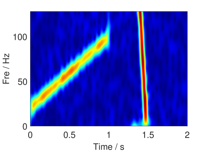
(a)

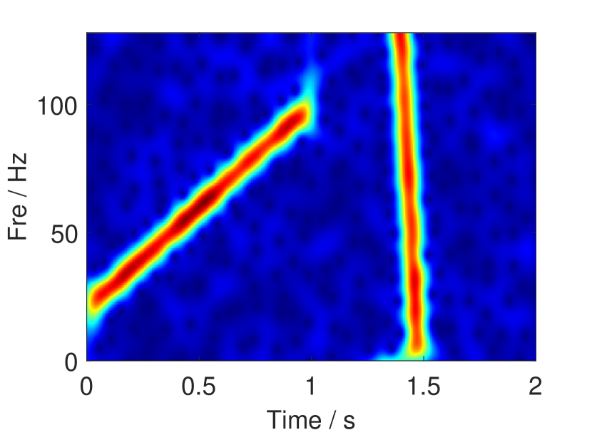
(b)

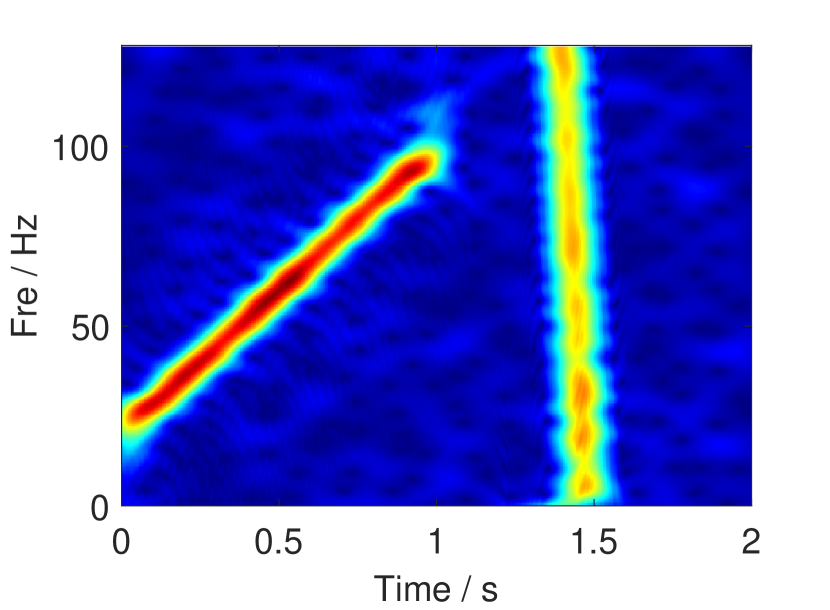
(c)

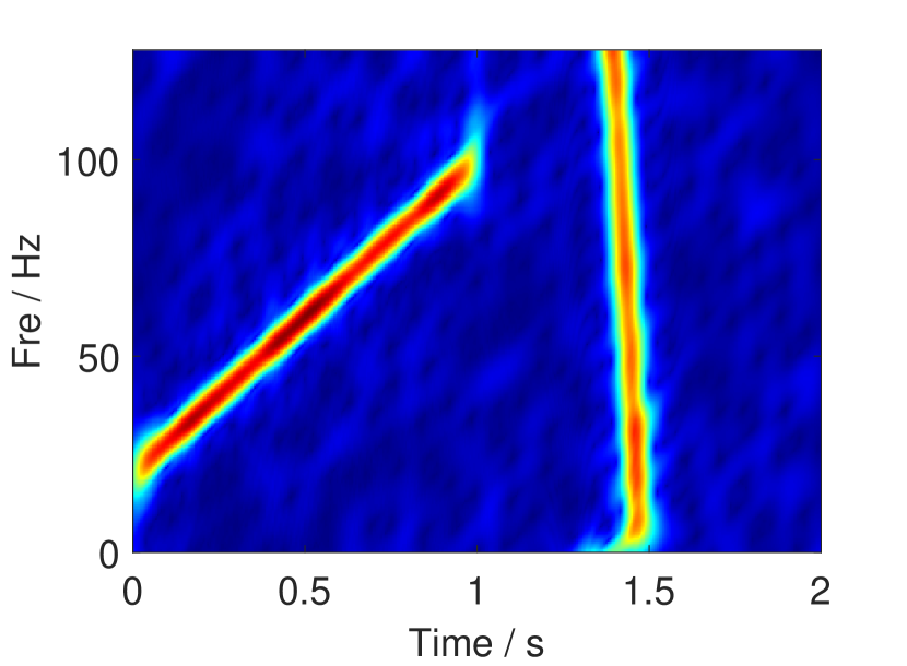
(d)

Figure 6: TF results using STFT and MrCT methods. (a) The STFT with $\sigma=0.1$, (b) the STFT with $\sigma=0.16$, (c) the STFT with $\sigma=0.25$, (d) the MrCT ($m=3$, $\sigma=0.1,0.16,0.25$).

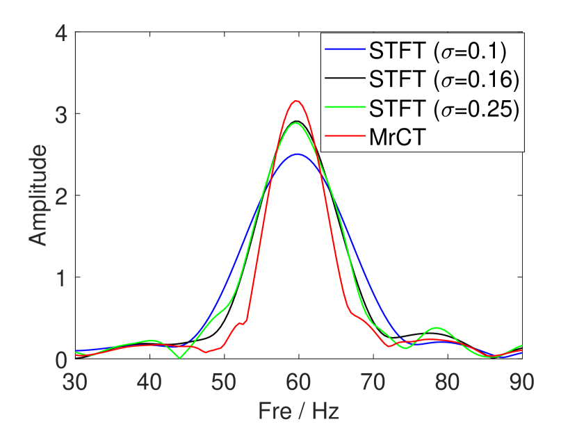
(a)

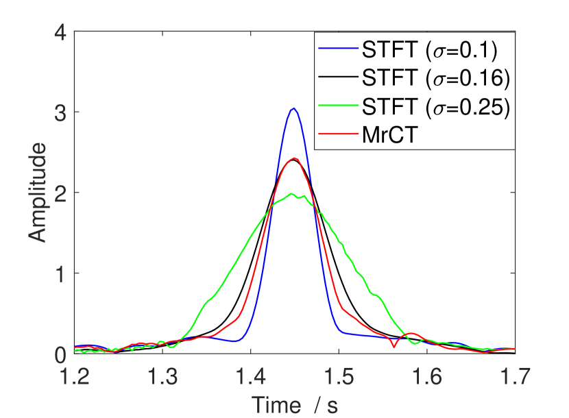
(b)

Figure 7: TF energy curves by selecting various frames. (a) Spectrum of the time frame $t=0.5$ s, (b) time evolution of the frequency bin Fre $=46$ Hz.

(a)

(b)

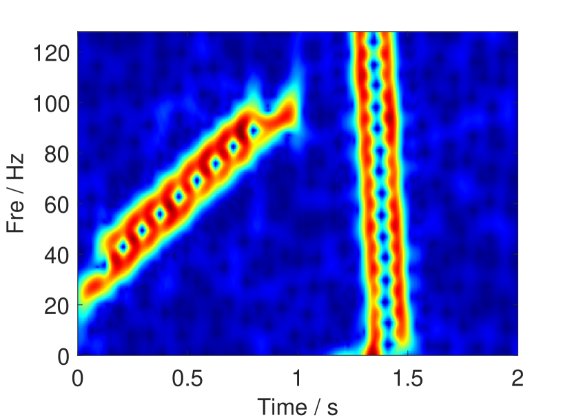
(c)

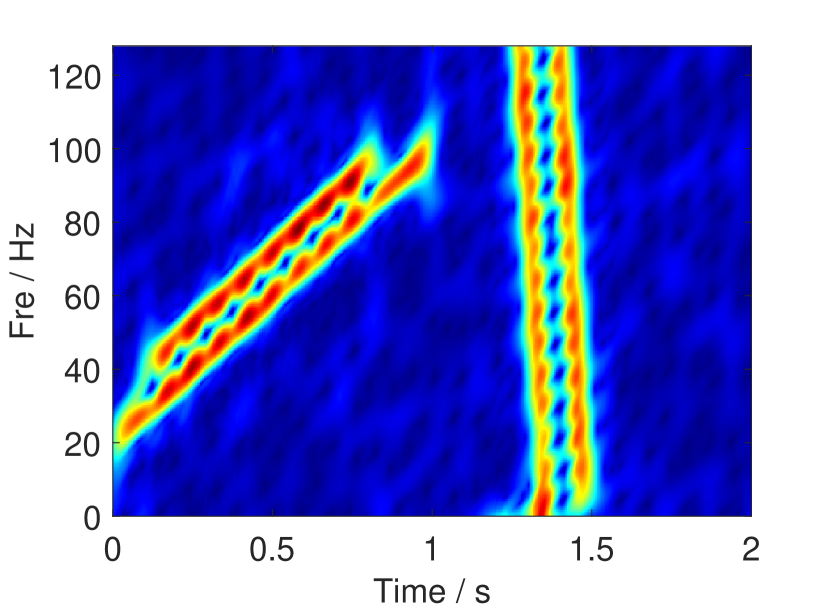
(d)

Figure 8: TF results of signal (42) using various analysis methods. (a) GLCT, (b) DACT, (c) MrSTFT, (d) MrCT.

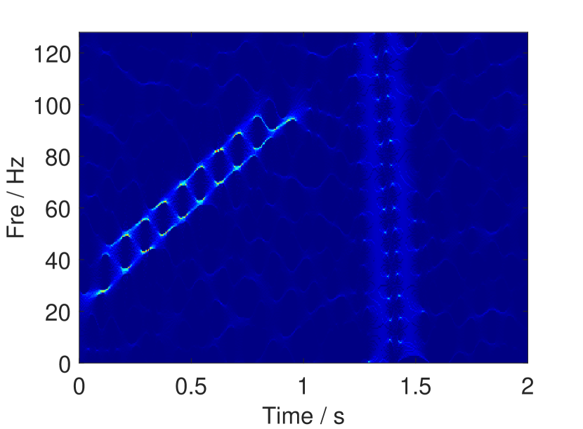
(a)

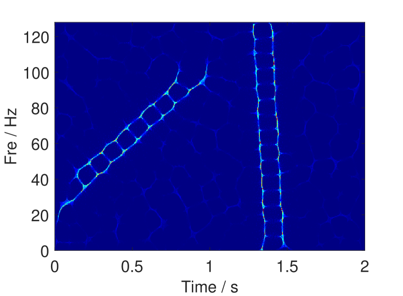
(b)

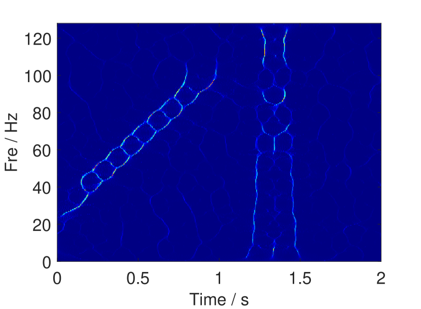
(c)

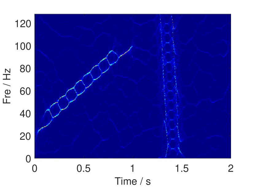
(d)

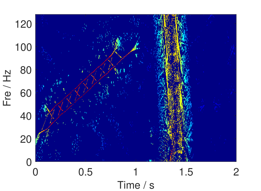
(e)

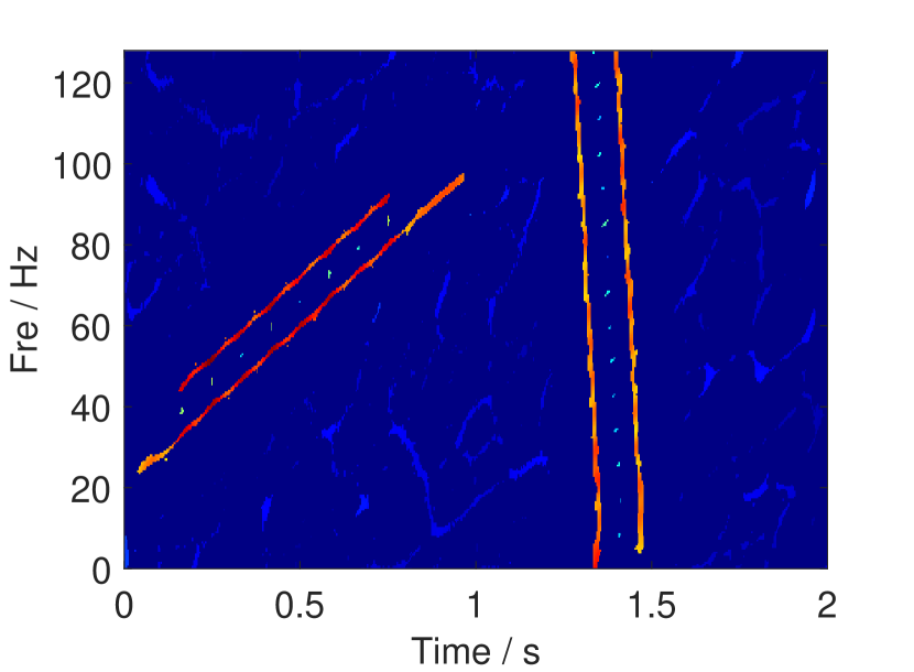
(f)

Figure 9: TF results by various post-processing methods. (a) TF plot by SST, (b) TF plot by RM, (c) TF plot by TSST, (d) TF plot by SSST, (e) TF plot by SECT, (f) TF plot by MrSECT.

Fig. 8 presents the TF representations by two adaptive CTs (i.e., GLCT and DACT) and two combined methods (i.e., MrSTFT and MrCT, here these two combinations use the same values of $\sigma$). From the results, we can see that the MrCT yields a high-concentration TF result, and the close components are clearly separated. While the other three methods lead to the TF plots being difficult to interpret. In addition, the computational times required for the GLCT, DACT, MrSTFT, and MrCT in addressing signal (42) are 0.312 s, 0.031 s, 0.027 s, and 0.041 s, respectively (the tested computer configuration: Intel Core i5-6600 3.30 GHz, 16.0 GB of RAM, and MATLAB version R2020b). The last three methods need much less calculation comparing with the GLCT in which the window function is adjusted at every TF location.

Fig. 9 displays the TF representations obtained by six TF post-processing methods, including the SST, RM, TSST, SSST, SECT, and MrSECT. It can be seen from the results that, there are heavy cross-terms between the first two modes in the TF plane for the first five methods. The MrSECT is clearly superior to others, yielding high concentration of both close components. Compared to the TF result of MrCT (see Fig. 8(d)), MrSECT effectively improves its TF readability.

V-B Example 2

Next, let us consider a four-component AM-FM signal with two cosine modulated modes and two impulse components as

$$\begin{split}&f(t)=f_{1}(t)+f_{2}(t)+f_{3}(t)+f_{4}(t)+n(t),\\ &f_{1}(t)=(1+0.05\cos(20\pi t))\cos(2\pi(9\sin(2\pi t)+80t)),\\ &f_{2}(t)=(1+0.1\cos(20\pi t))\cos(2\pi(9\sin(2\pi t)+115t)),\\ &f_{3}(t)=5\exp(-10000\pi(t-0.46)^{2})\cos(340\pi t),\\ &f_{4}(t)=5\exp(-10000\pi(t-0.52)^{2})\cos(340\pi t),\end{split}$$ (43)

where $n(t)$ is the Gaussian noise with the SNR$=8$ dB. The sampling frequency is 512 Hz, and time duration is [0 1s].

Fig. 10 provides the TF plots of signal (43) obtained by the GLCT, DACT, MrSTFT, and MrCT ($m=6$). It is seen that serious cross-terms appear between the close components in the TF representations of GLCT and DACT, and these two methods are unable to fully segregate time and frequency. By contrast, MrSTFT and MrCT provide a faithful local representation, with high resolution in both time and frequency. Compared to MrSTFT, the MrCT has more concentrated TF energy at the modulation part (see TF plot in the time interval [0.1, 0.3], [0.7, 0.9]), showing good performance in handling cosine modulation signals.

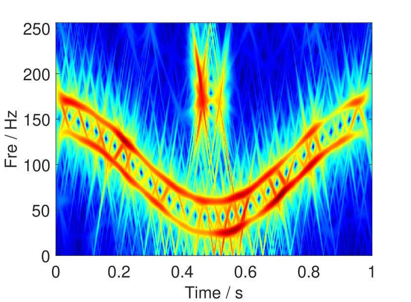
(a)

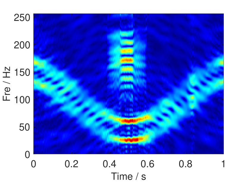
(b)

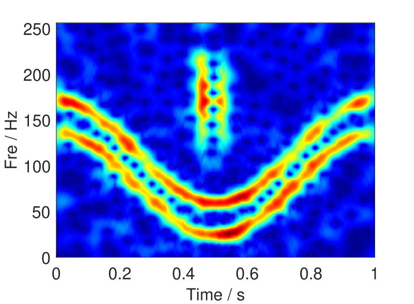
(c)

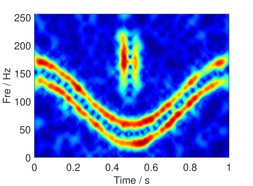
(d)

Figure 10: TF results of signal (43) using various analysis methods. (a) GLCT, (b) DACT, (c) MrSTFT, (d) MrCT.

(a)

(b)

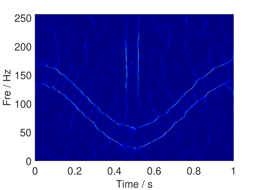
(c)

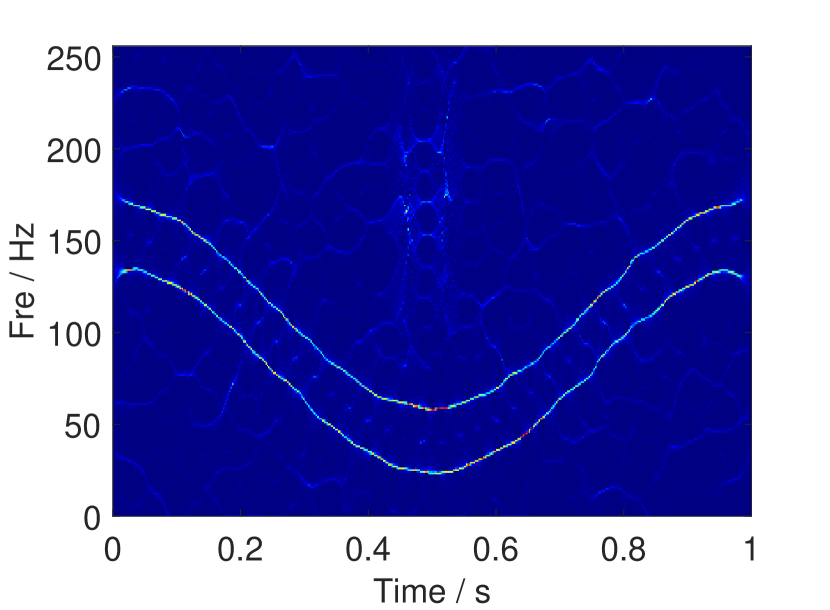
(d)

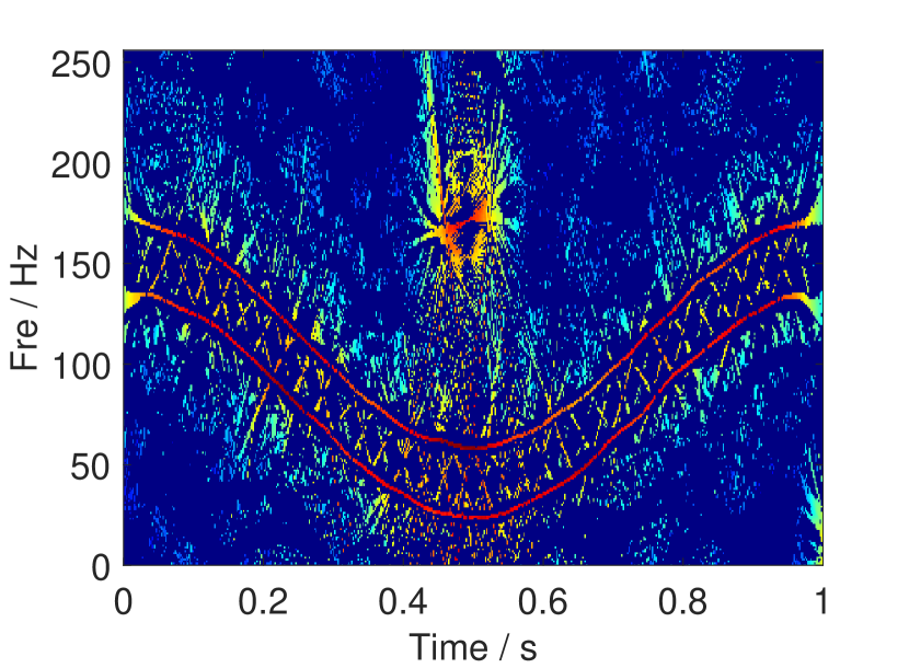
(e)

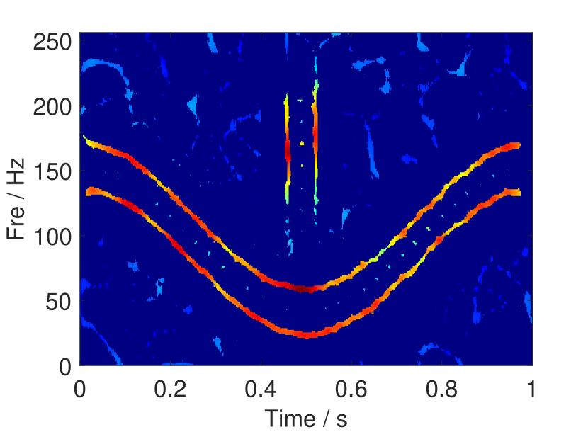
(f)

Figure 11: TF results by various post-processing methods. (a) TF plot by SST, (b) TF plot by RM, (c) TF plot by TSST, (d) TF plot by SSST, (e) TF plot by SECT, (f) TF plot by MrSECT.

Fig. 11 gives the TF representations generated by the six post-processing methods. It clearly shows that the TF result of SST is blurred. The SSST and SECT provide the TF plots with high energy concentration for $f_{1}(t)$ and $f_{2}(t)$, but fail to characterize impulsive signals effectively. The TSST provides a better TF localization for the transient signals, while degrading the TF sharpness of the cosine modulation signals at the stationary part (see TF plot in the time interval [0.4, 0.6]). The RM is to reassign the spectrogram from the TF direction such that the corresponding time resolution is more concentrated than SST-based methods, but it is not as clear as the MrSECT. By comparison, the MrSECT has the best TF readability in handling signal (43). It should be pointed out that the proposed MrSECT is subject to the boundary effects, missing a small amount of boundary information when pursuing a high-concentration TF representation.

V-C Application

A typical biomedical signal, ECG signal from the BIDMC the Dataset [71], is employed to validate our proposed method. The sample rate of the ECG signal is 125 Hz. About 8 s ECG segment and its STFT are displayed in Fig. 12.

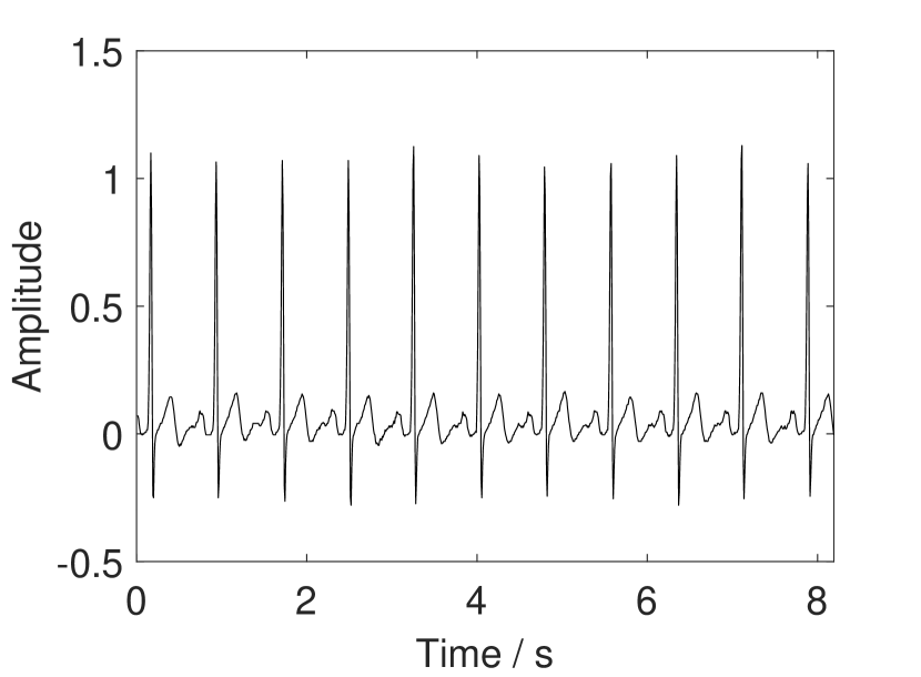
(a)

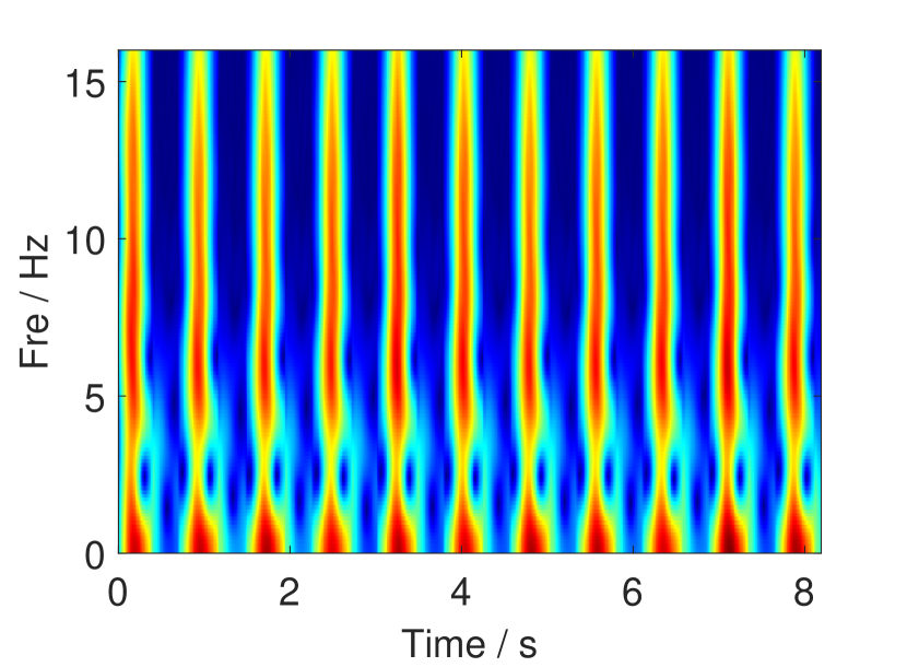
(b)

Figure 12: The time series of the ECG signal and its spectrogram.

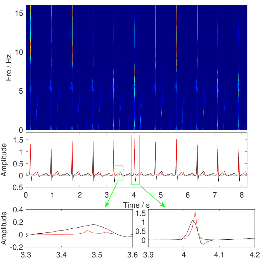
(a)

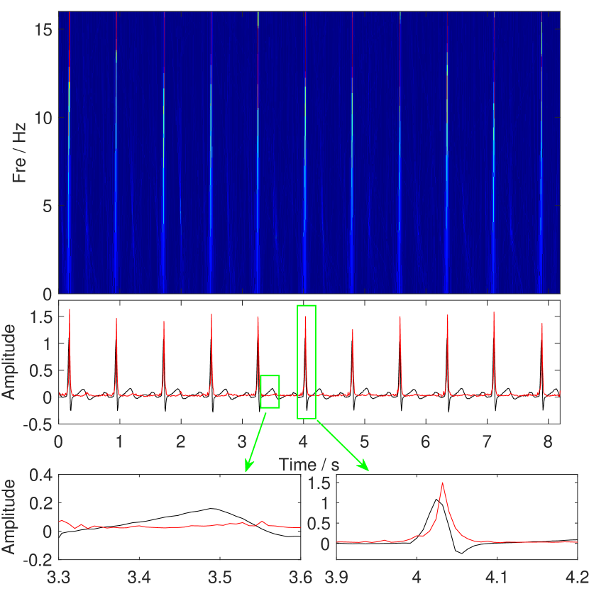
(b)

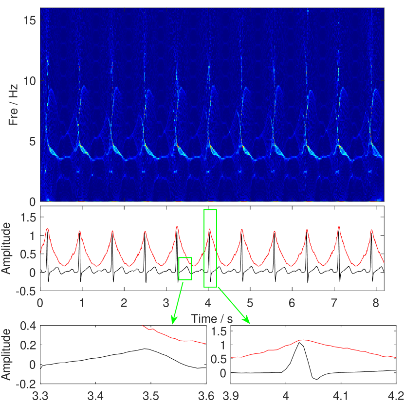
(c)

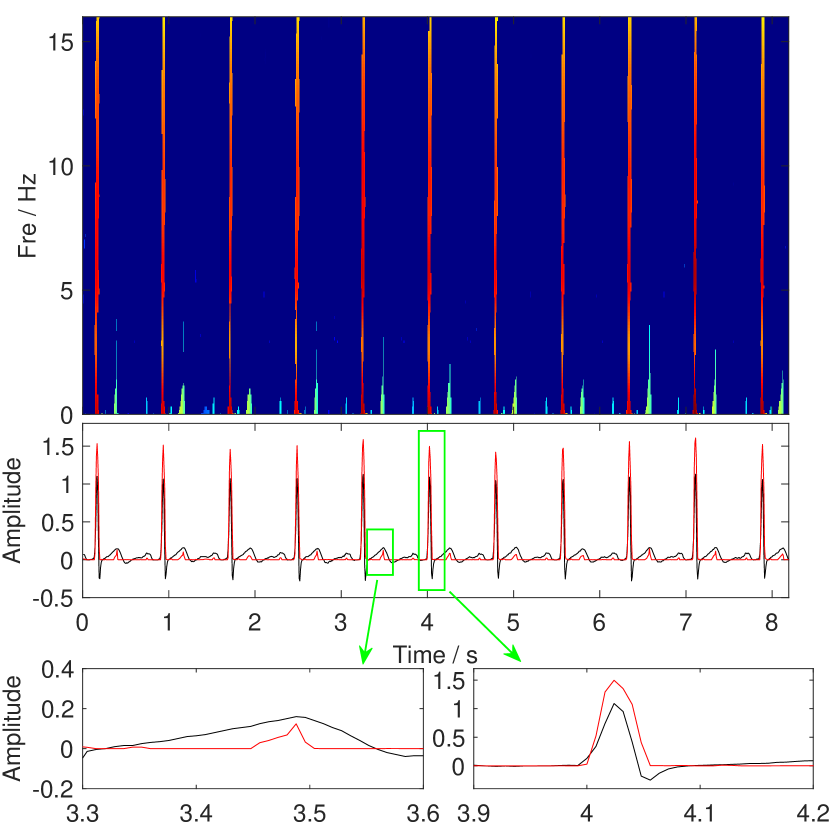
(d)

Figure 13: The ECG’s analysis results calculated by different methods: (a) RM, (b) TSST, (c) SSST, (d) MrSECT. In the below of each TF result, there are time distribution of each TF representation (red -), the original signal (blak -), and locally-zoomed results, as marked with the green boxes.

Fig. 13 shows the analysis results of ECG signal estimated by four different methods: (a) RM, (b) TSST, (c) SSST, (d) MrSECT. The SSST presents a blurry TF representation, based on which, it is difficult to make further analysis and judgment. Fig. 13(a,b,d) indicate that RM, TSST, and MrSECT achieve good energy concentration for the spikes of the ECG signal. These methods (especially the MrSECT) can resolve the spikes and describe the transient characteristics clearly. We also give the time-domain marginal distribution of each TF result as well as locally-zoomed results for the parts marked with the green boxes. As illustrated in Fig. 13, the result obtained by our MrSECT approach achieves superior effectiveness in TF dynamic estimation because it reflects the dynamic change of the ECG signal more accurately.

VI Conclusion

In this paper, we focused on improving the TF resolution of the standard chirplet transform (CT) for multi-component non-stationary signal analysis. We theoretically analyzed the effect of the chirp-based Gaussian window on the CT and compared the CT with the rotation-window CT. The given parameters analysis showed some interesting results like that a narrow window limits the matching capacity of chirp basis, and provided theoretical instruction for CT to choose suitable parameters to obtain a high-resolution TF representation. To overcome the limitation of CT in dealing with signals consisting of a mixture of chirps and pulses, we proposed the multi-resolution chirplet transform (MrCT) by computing the geometric mean of multiple CTs, which takes advantage of multiple estimates at a range of temporal resolutions and frequency bandwidths and localizes the signal in both time and frequency better than it is possible with any single CT. Moreover, based on the combined IF equation, we developed the multi-resolution synchroextracting chirplet transform (MrSECT) to further improve the readability of the proposed MrCT. The numerical results and real signal application confirmed the effectiveness of the proposed approaches.

Although the MrCT and MrSECT have a good performance in addressing closely-spaced signals, some works should be considered.

• The noise robustness analysis of the proposed MrCT approach, as well as a deeper understanding of the influence of noise on the combined IF equation, should be discussed.

• The MrSECT is subject to the boundary effects, how to minimize the boundary effects based on forecasting techniques is worthy of consideration.

• The application to other real-life signals (e.g., radar signal [4], mechanical vibration signal [32]) needs to be further investigated.

References

- [1] X. Pan, D. Zhang, P. Zhang, “Fracture detection from Azimuth-dependent seismic inversion in joint time-frequency domain”, Sci Rep., vol. 11, p. 1269, 2021.
- [2] D. Song, Z. Chen, H. Chao, Y. Ke, W. Nie, “Numerical study on seismic response of a rock slope with discontinuities based on the time-frequency joint analysis method”, Soil Dyn. Earthq. Eng., vol. 133, p. 106112, 2020.
- [3] M.G. Amin, Y.D. Zhang, F. Ahmad, K. Ho, “Radar signal processing for elderly fall detection: The future for in-home monitoring”, IEEE Signal Process. Mag., vol. 33, no. 2, pp. 71-80, 2016.
- [4] A.A. Ahmad, S. Lawan, M. Ajiya, Z.Y. Yusuf, L. Bello, “Extraction of the pulse width and pulse repetition period of linear FM radar signal using time-frequency analysis”, Journal of Advances in Science and Engineering, vol. 3, no. 1, pp. 1-8, 2020.
- [5] V.V. Moca, H. Bârzan, A. Nagy-Dăbâcan, R. CMure\textcommabelowsan, “Time-frequency super-resolution with superlets”, Nat. Commun., vol. 12, p. 337, 2021.
- [6] H-T. Wu, “Current state of nonlinear-type time-frequency analysis and applications to high-frequency biomedical signals”, Current Opinion in Systems Biology, vol. 23, pp. 8-21, 2020.
- [7] Z.K. Peng, F.L. Chu, P.W. Tse, “Detection of the rubbing-caused impacts for rotor-stator fault diagnosis using reassigned scalogram”, Mech. Syst. Signal Process., vol. 19, pp.391-409, 2005.
- [8] N.G. Nikolaou, I.A. Antoniadis, “Rolling element bearing fault diagnosis using wavelet packets”, NDT & E International, vol. 35, no. 3, pp. 197-205, 2012.
- [9] G. Han, S. Li, X, Xue, X. Zheng, “Photonic chirp rates estimator for piecewise linear frequency modulated waveforms based on photonic self-fractional Fourier transform”, Optics Express, vol. 28, no. 15, pp. 21783-21791, 2020.
- [10] L. Cohen, Time-Frequency Analysis, Prentice-Hall, Englewood Cliffs, NJ, 1995.
- [11] M.R. Portnoff, “Time-frequency representation of digital signals and systems based on short-time Fourier analysis”, IEEE Trans. Acoust. Speech Signal Process., vol. 28, no. 1, pp. 55-69, 1980.
- [12] A. Grossmann, J. Morlet, “Decomposition of hardy functions into square integrable wavelets of constant shape”, SIAM J. Math. Anal., vol. 15, no. 4, pp. 723-736, 1984.
- [13] S. Mann, S. Haykin, “The chirplet transform: physical considerations,” IEEE Trans. Signal Process., vol. 43, no. 11, pp. 2745-2761, 1995.
- [14] T. Claasen, W. Mecklenbräuker, “The Wigner distribution-A tool for time-frequency signal analysis-Part I: Continuous-time signals”, Philips J. Res., vol. 35, pp. 217-250, 1980.
- [15] I. Shafi, J. Ahmad, S.I. Shah, F.M. Kashif, “Techniques to obtain good resolution and concentrated time-frequency distributions: a review”, EURASIP J. Adv. Signal Process., vol. 2009, p. 673539, 2009.
- [16] B. Boashash, Time-Frequency Signal Analysis and Processing: A comprehensive Reference, Elsevier, Oxford, UK, 2003.
- [17] K. Kodera, R. Gendrin, C. Villedary, “Analysis of time-varying signals with small BT values”, IEEE Trans. Acoust. Speech Signal Process., vol. 26, pp. 64-76, 1978.
- [18] F. Auger, P. Flandrin, “Improving the readability of time-frequency and time-scale representations by the reassignment method”, IEEE Trans. Signal Process., vol. 43, no. 5, pp. 1068-1089, 1995.
- [19] I. Daubechies, S. Maes, “A nonlinear squeezing of the continuous wavelet transform based on auditory nerve models”, in: Wavelets in Medicine and Biology, CRC Press, 1996, pp. 527-546.
- [20] I. Daubechies, J.F. Lu, H.T. Wu, “Synchrosqueezed wavelet transforms: an empirical mode decomposition-like tool”, Appl. Computat. Harmon. Anal., vol. 30, pp. 243-261, 2011.
- [21] G. Thakur, H.T. Wu, “Synchrosqueezing-based recovery of instantaneous frequency from nonuniform samples”, SIAM J. Math. Anal., vol. 43, no. 5, pp. 2078-2095, 2012.
- [22] H. Yang, L. Ying, “Synchrosqueezed curvelet transform for two dimensional mode decomposition”, SIAM. J. Math. Anal., vol. 46, no. 3, pp. 2052-2083, 2014.
- [23] Z. Huang, J. Zhang, Z. Zou, “Synchrosqueezing S-transform and its application in seismic spectral decomposition”, IEEE Trans. Geosci. Remote Sens., vol. 54, no. 2, pp. 817-825, 2016.
- [24] X. Zhu, Z. Zhang, Z. Li, J. Gao, X. Huang, G. Wen, “Multiple squeezes from adaptive chirplet transform”, Signal Process., vol. 163, pp. 26-40, 2019.
- [25] C. Li, M. Liang, “A generalized synchrosqueezing transform for enhancing signal time-frequency representation”, Signal Process., vol. 92, pp. 2264-2274, 2012.
- [26] T. Oberlin, S. Meignen, V. Perrier, “Second-order synchrosqueezing transform or invertible reassignment? Towards ideal time-frequency representations”, IEEE Trans. Signal Process., vol. 63, no. 5, pp. 1335-1344, 2015.
- [27] S. Wang, X. Chen, G. Cai, B. Chen, X. Li, Z. He, “Matching demodulation transform and synchrosqueezing in time-frequency analysis”, IEEE Trans. Signal Process., vol. 62, no. 1, pp. 69-84, 2014.
- [28] D.H. Pham, S. Meignen, “High-order synchrosqueezing transform for multicomponent signals analysis-with an application to gravitational-wave signal”, IEEE Trans. Signal Process., vol. 65, no. 12, pp. 3168-3178, 2017.
- [29] G. Yu, Z. Wang, P. Zhao, “Multi-synchrosqueezing transform”, IEEE Trans. Ind. Electron., vol. 66, no. 7, pp. 5441-5455, 2019.
- [30] X. Zhu, Z. Zhang, J. Gao, B. Li, Z. Li, X. Huang, G. Wen, “Synchroextracting chirplet transform for accurate IF estimate and perfect signal reconstruction”, Dig. Signal Process., vol. 93, pp. 172-186, 2019.
- [31] D. He, H. Cao, S. Wang, X. Chen, “Time-reassigned synchrosqueezing transform: The algorithm and its applications in mechanical signal processing”, Mech. Syst. Signal Process., vol. 117, pp. 255-279, 2019.
- [32] G. Yu, T. Lin, “Second-order transient-extracting transform for the analysis of impulsive-like signals”, Mech. Syst. Signal Process., vol. 147, p. 107069, 2021.
- [33] J. Zhong, Y. Huang, “Time-frequency representation based on an adaptive short-time Fourier transform”, IEEE Trans. Signal Process., vol. 58, no. 10, pp. 5118-5128, 2010.
- [34] D.L. Jones, T.W. Parks, “A high resolution data-adaptive time-frequency representation”, IEEE Trans. Acoust. Speech Signal Process., vol. 38, no. 12, pp. 2127-2135, 1990.
- [35] S.C. Pei, S.G. Huang, “STFT with adaptive window width based on the chirp rate”, IEEE Trans. Signal Process., vol. 60, no. 8, pp. 4065-4080, 2012.
- [36] S.C. Pei, S.G. Huang, “Adaptive STFT with chirp-modulated Gaussian window”, 2018 IEEE International Conference on Acoustics, Speech and Signal Processing (ICASSP), Calgary, AB, Canada, 2018, pp. 4354-4358.
- [37] L. Li, H. Cai, H. Han, Q. Jiang, H. Ji, “Adaptive short-time Fourier transform and synchrosqueezing transform for non-stationary signal separation”, Signal Process., vol. 66, p. 107231, 2020.
- [38] H.X. Chen, Patrick S.K. Chua, G.H. Lim, “Adaptive wavelet transform for vibration signal modelling and application in fault diagnosis of water hydraulic motor”, Mech. Syst. Signal Process., vol. 20, no. 8, pp. 2022-2045, 2006.
- [39] J. Yao, Y.T. Zhang, “Bionic wavelet transform: a new time-frequency method based on an auditory model”, IEEE Trans. Biomed. Eng., vol. 48, no. 8, pp. 856-863, 2001.
- [40] E. Sejdić, I. Djurović, J. Jiang, “A window width optimized S-transform”, EURASIP J. Adv. Signal Process., vol. 2008, p. 672941, 2007.
- [41] R. Lin, Z. Liu, Y. Jin, “Instantaneous frequency estimation for wheelset bearings weak fault signals using second-order synchrosqueezing S-transform with optimally weighted sliding window”, ISA Transactions, 2021, doi: 10.1016/j.isatra.2021.01.010.
- [42] L. Stanković, “A method for improved distribution concentration in the time-frequency analysis of multicomponent signals using the L-Wigner distribution”, IEEE Trans. Signal Process., vol. 43, no. 5, pp. 1262-1268, 1995.
- [43] B. Boashash, P. O’Shea, “Polynomial Wigner-Ville distributions and their relationship to time-varying higher order spectra”, IEEE Trans. Signal Process., vol. 42, no. 1, pp. 216-220, 1994.
- [44] V. Katkovnik, “Local polynomial approximation of the instantaneous frequency: asymptotic accuracy”, Signal Process., vol. 52, no. 3, pp. 343-356, 1996.
- [45] D.L. Jones, R.G. Baraniuk, “An adaptive optimal-kernel time-frequency representation”, IEEE Trans. Signal Process., vol. 43, no. 10, pp. 2361-2371, 1995.
- [46] N.A. Khan, B. Boashash, “Instantaneous frequency estimation of multi-component nonstationary signals using multiview time-frequency distributions based on the adaptive fractional spectrogram”, IEEE Signal Process. Lett., vol. 20, no.2, pp. 157-160, 2013.
- [47] N.A. Khan, B. Boashash, “Multi-component instantaneous frequency estimation using locally adaptive directional time frequency distributions”, Int. J. Adapt. Control Signal Process., vol. 30, pp. 429-442, 2016.
- [48] M. Mohammadi, A.A. Pouyan, N.A. Khan, V. Abolghasemi, “Locally optimized adaptive directional time-frequency distributions”, Circuits Syst. Signal Process., vol. 37, no. 8, pp. 3154-3174, 2018.
- [49] H. Zhang, G. Hua, Y. Xiang, “Enhanced time-frequency representation and mode decomposition”, IEEE Trans. Signal Process., 2021, doi: 10.1109/TSP.2021.3093786.
- [50] S. Cheung, J.S. Lim, “Combined multiresolution (wide-band/narrow-band) spectrogram”, IEEE Trans. Signal Process., vol. 40, pp. 975-977, 1992.
- [51] P. Loughlin, J. Pitton, B. Hannaford, “Approximating time-frequency density functions via optimal combinations of spectrograms”, IEEE Signal Process. Lett., vol. 1, pp. 199-202, 1994.
- [52] D. Mihovilovic, R. Bracewell, “Adaptive chirplet representation of signals on time-frequency plane”, Electron. Lett., vol. 27, no. 13, pp. 1159-1161, 1991.
- [53] F. Millioz, M. Davies, “Sparse detection in the chirplet transform: application to FMCW radar signals”, IEEE Trans. Signal Process., vol. 60, no. 6, pp. 2800-2813, 2012.
- [54] K. Abratkiewicz, “Double-adaptive chirplet transform for radar signature extraction”, IET Radar Sonar & Navigation, vol. 14, no. 10, pp. 1463-1474, 2020.
- [55] S.K. Ghosh, R.N. Ponnalagu, R.K. Tripathy, U. Rajendra Acharya, “Automated detection of heart valve diseases using chirplet transform and multiclass composite classifier with PCG signals”, Computers in Biology and Medicine, vol. 118, p. 103632, 2020.
- [56] G. Yu, Y. Zhou, “General linear chirplet transform”, Mech. Syst. Signal Process., vol. 70-71, pp. 958-973, 2016.
- [57] M. Li, T. Wang, F. Chu, Q. Han, Z. Qin, M. Zuo, “Scaling-basis chirplet transform”, IEEE Trans. Ind. Electron., vol. 68, no. 9, pp. 8777-8788, 2021.
- [58] K. Czarnecki, D. Fourer, F. Auger, M. Rojewski, “A fast time-frequency multiwindow analysis using a tuning directional kernel”, Signal Process., vol. 147, pp. 110-119, 2018.
- [59] Y. Miao, H. Sun, J. Qi, “Synchro-compensating chirplet transform”, IEEE Signal Process. Lett., vol. 25, no. 9, pp. 1413-1417, 2018.
- [60] L. Angrisani, M. D’Arco, R.S.L. Moriello, M. Vadursi, “Warblet transform based method for instantaneous frequency measurement on multicomponent signals”, 2004 IEEE International Frequency Control Symposium and Exposition, Montreal, QC, Canada, 2004, pp. 500-508.
- [61] Y. Yang, Z. Peng, G. Meng, W. Zhang, “Characterize highly oscillating frequency modulation using generalized warblet transform”, Mech. Syst. Sig. Process., vol. 26, pp. 128-140, 2012.
- [62] Z. Peng, G. Meng, F. Chu, Z. Lang, W. Zhang, Y. Yang, “Polynomial chirplet transform with application to instantaneous frequency estimation”, IEEE Trans. Instrum. Meas., vol. 60, no. 9, pp. 3222-3229, 2011.
- [63] Y. Yang, Z. Peng, G. Meng, W. Zhang, “Spline-kernelled chirplet transform for the analysis of signals with time-varying frequency and its application”, IEEE Trans. Ind. Electron., vol. 59, no. 3, pp. 1612-1621, 2012.
- [64] L. Li, N.N. Han, Q.T. Jiang, C.K. Chui, “A separation method for multicomponent non-stationary signals with crossover instantaneous frequencies”, arXiv2010.01498, 2020.
- [65] C.K. Chui, Q. Jiang, L. Li, J. Lu, “Time-scale-chirp-rate operator for recovery of non-stationary signal components with crossover instantaneous frequency curves”, Appl. Computat. Harmon. Anal., Vol. 54, pp. 323-344, 2021.
- [66] X. Zhu, Z, Zhang, J. Gao, “Three-dimension extracting transform”, Signal Process., vol. 179, p. 107830, 2021.
- [67] H.M. Ozaktas, D. Mendlovic, “Fourier transforms of fractional order and their optical interpretation”, Opt. Commun., vol. 101, no. 3, pp. 163-169, 1993.
- [68] J. Shi, J. Zheng, X. Liu, W. Xiang, Q. Zhang, “Novel short-time fractional Fourier transform: theory, implementation, and applications”, IEEE Trans. Signal Process., vol. 68, pp. 3280-3295, 2020.
- [69] D.D. Lee, H.S. Seung, “Algorithms for nonnegative matrix factorization”, In Advances in Neural and Information Processing Systems 13, London, England, 2001, pp. 556-562.
- [70] X.G. Xia, “Discrete chirp-Fourier transform and its application to chirp rate estimation”, IEEE Trans. Signal Process., vol. 48, no. 11, pp. 3122-3133, 2000.
- [71] A.L. Goldberger, L.A. Amaral, L. Glass, J.M. Hausdorff, P.C. Ivanov, R.G.Mark, J.E. Mietus, G.B.Moody, C.K.Peng, H.E. Stanley, “PhysioBank, PhysioToolkit, and PhysioNet: components of a new research resource for complex physiologic signals”, Circulation, vol. 101, pp. E215-E220, 2000.