Transformer-Encoder-GRU (T-E-GRU) for Chinese Sentiment Analysis on Chinese Comment Text

Abstract

Chinese sentiment analysis (CSA) has always been one of the challenges in natural language processing due to its complexity and uncertainty. Transformer has succeeded in capturing semantic features, but it uses position encoding to capture sequence features, which has great shortcomings compared with the recurrent model. In this paper, we propose T-E-GRU for Chinese sentiment analysis, which combine transformer encoder and GRU. We conducted experiments on three Chinese comment datasets. In view of the confusion of punctuation marks in Chinese comment texts, we selectively retain some punctuation marks with sentence segmentation ability. The experimental results show that T-E-GRU outperforms classic recurrent model and recurrent model with attention.

1 Introduction

Sentiment analysis has become one of the most active fields in natural language processing (NLP) feldman2013techniques ; zhang2018deep . With the development of sentiment analysis, the research is not only limited to the computer field, but also expanded to management, social science, etc. Its potential commercial value has also attracted the attention of all sectors of society. With the development of GPU, sentiment analysis methods based on machine learning and deep learning gradually occupy the dominant position and continue to achieve the state-of-the-art performance.

The earliest CSA is based on sentiment dictionary, which judges the sentiment tendency of the text through its vocabulary. But none of them have the ability to capture sequence features. Recurrent neural network (RNN) proposed by Jeffrey L Elman  preRNN is one of the effective methods to alleviate this defect, but it was accompanying by vanishing/exploding gradient problem bengio1994Long-term-dependencies-diffcult . Subsequently, a series of recurrent models based on RNN were proposed to address these problems, such as long short-term memory (LSTM) hochreiter1997LSTM , gate recurrent neural network (GRU) cho2014learningGRU , etc. However, the vanishing/exploding gradient problem on long sequence is still one of its most important limitations. To address the vanishing/exploding problems, Bahdanau et al. bahdanau2014Attention-first proposed the attention mechanism, which assigns weights to input sequence to make the model pay more attention to keywords. After that, the models with attention continues to achieve state-of-the-art performances. In particular, in 2017, Vaswani et al. vaswani2017Transformer proposed scaled dot-product attention which has become one of the effective ways to apply attention mechanism and transformer model. Transformer and its variants have achieved the state-of-the-art performances on basic problems in many fields BERT ; vaswani2017Transformer . Transformer-Encoder realizes the extraction of sequence features through position encoding (PE), which still has a gap with the natural sequence feature extractor such as RNN.

Although sentiment analysis has made remarkable achievements in recent years, most of them are based on English. Compared with English, Chinese natural language processing is more challenging. On the one hand, Chinese has more complicated vocabulary and semantics. On the other hand, Chinese text semantics are more dependent on context. Inspired by the powerful global feature extraction ability of attention & transformer and the powerful sequence feature extraction ability of recurrent model, we proposed Transformer-Encoder-GRU (T-E-GRU) which combine the GRU with the structure of transformer, and use it for sentiment analysis of Chinese reviews. We compare it with recurrent model, recurrent model with attention, etc. The results show that our model achieves better results.

The main contributions of this paper are summarized as following:

1. We proposed a novel model called T-E-GRU based on GRU and transformer encoder, which is exactly suitable for CSA.

2. Focus on the complexity and confusion of punctuation in Chinese comments, we have selectively retained some punctuation that has the ability to clauses.

3. Extensive experiment demonstrate that T-E-GRU achieves better effect on CSA.

2 Related Work

2.1 Chinese Text To sequence

In Chinese natural language processing, Chinese word segmentation (CWS) is a basic and important task, which segments text into independent word units. Compared with the natural delimiter spaces in English, Chinese has no formal delimiters and no strict division method, and even sometimes the division method depends on the context. The main disadvantages of dictionary-based word segmentation algorithms such as forward maximum matching (FMM), backward maximum matching (BMM), and bi-direction matching (BiMM) are slow in matching and cumbersome implementation of supplementing unrecorded words CWS10yearReview . Based on statistical machine learning algorithms, the main idea is that the more adjacent characters appear in the context at the same time, the more likely they are to form a word. The current main models are: N-gram model (N-gram) N-gram , hidden Markov model (HMM) HMM , condition random field (CRF) CRF , RNN variant model LSTM-CWS ; Bi-LSTM-CWS . Various open CWS libraries such as Jieba, FoolNLTK, LTP, etc. have performed well in CWS. Although some people have raised doubts about the necessity of CWS in deep learning WS-is-necessary , most of the state-of-the-art models are based on CWS.

The simplest way to represent words is to use one-hot encoding which brings curse of dimensionality, semantic gap and poor scalability. Fighting the curse of dimensionality, Bengio Y et al. proposed a method of using low-dimensional vector to represent vocabulary proposed-Embedding . Word Embedding is a by-product of their model. In 2013, Tomas Mikolov proposed word2Vec word2Vec , which is a faster and better method for training word embedding model. There are two algorithms: skip-grams and continuous bag-of-words (CBOW) CBOW , both of which based on N-gram model.The N-gram model assumes that a word is only related to N surrounding words. This assumption determines that the disadvantage is insufficient use of global information. Jeffrey Pennington et al. proposed global vectors for Word representation (GloVe) which considers both global and local information glove . However, the word representation mentioned above is a static model, which cannot cope with the situation where a word has multiple meanings. In 2018, Peters M E et al. proposed embeddings from language model (ELMO) ELMO by using bidirectional LSTM. Since transformer has been proved to have powerful feature extraction ability in many researches vaswani2017Transformer , generative pre-training (GPT) was proposed GPT . It replaces LSTM in ELMO with transformer. Although GPT uses a unidirectional language model, it achieves the best results in 9 of the 12 tasks in NLP. In 2019, Devlin et al. proposed bidirectional encoder representations from transformers (BERT) BERT which replace unidirectional with bidirectional language models, and also combined with the tricks of CBOW. BERT, as synthesis of word representation model in recent years, achieved state-of-the-art performances in multiple NLP basic tasks.

2.2 Recurrent models

Recurrent model is one of the effective methods for processing sequence input. In 1990, neuroscientist Jeffrey L Elman proposed RNN which is based on the Jordan Network preRNN back-propagation (BP) BP . However, vanishing/exploding gradient problem on long sequence comes with RNN bengio1994Long-term-dependencies-diffcult . In 1997, Hochreiter et al. proposed LSTM, which can alleviate this problem by introducing delicate gate mechanism hochreiter1997LSTM . However, LSTM often has overfitting on some tasks due to the complexity of its structure. Cho et al. simplified the gate of LSTM and propose GRU cho2014learningGRU . GRU has the same performance as LSTM but with fewer parameters. RNN, LSTM and GRU have become the most important recurrent models, but none of them can completely solve the vanishing/exploding gradient problem. Up to now, methods to improve RNN from different perspectives are still proposed one after another liu2021selfish .

2.3 Attention and Transformer

In 2014, Mnih V et al. applied attention mechanism on RNN to solve image classification tasks cv_Att . Then, attention was used as a way to solve the information overload problem in NLP tasks. Bahdanau et al. extended the basic seq2seq model with attention, and it yields good results on longer sentences bahdanau2014Attention-first . Then Cheng proposed intra-attention Att-breakout-Seq2seq , which broke the limitation of attention mechanism used in seq2seq. Many researches bahdanau2014Attention-first ; Att-breakout-Seq2seq ; cv_Att ; RecurrentAttNet-AspectSentimentAnalysis show that attention is effective in long sequence information loss. Vaswani et al. completely abandoned RNN and CNN to build transformer which is entirely based on the fully-connected layer and attention mechanism vaswani2017Transformer . In 2020, Zhou H et al. proposed probsparse self-attention mechanism and informer, and this model achieved high prediction capacity in the long sequence time-series forecasting zhou2020informer . Transformer is divided into two parts: encoding and decoding. Transformer-encoder uses position encoding to make the model understand sequence features. T-E-GRU replaces the position encoding with GRU, which has similar performance to LSTM. So T-E-GRU has the advantages of transformer-encoder and recurrent model, which will be more suitable for CSA.

2.4 Chinese sentiment analysis

Chinese sentiment analysis is very challenging due to the complexity of Chinese. A plain method is based on the n-gram model and syntax tree, using some classic machine learning classification models such as naive Bayesian (NB), support vector machine (SVM), etc. for CWS zou2015sentiment . The performance of their model were unsatisfactory. Ding et al. ding2008holistic also proposed a method of matching sentiment words in specific field for CSA. J Liang et al. liang2015polarity combined polarity shifting and LSTM for CSA. Xiao Z xiao2016chinese proposed bidirectional LSTM with word embedding for CSA. Their model already has high accuracy in CSA. As the attention mechanism and transformer were proposed, a series of models were for CSA. Bin et al. bin2017aspect proposed multi-attention convolutional neural network (CNN) for aspect-based sentiment analysis. In 2019, Shi, Xiaoming et al. shi2019attention proposed attention-based bidirectional hierarchical LSTM networks. In 2021, Wang, Shitao et al. wang2021bigru proposed bigru-multi-head self-attention network for CSA. In addition, many state-of-the-art models based on transformer or BERT have been proposed for CSA tang2021chinese ; zhu2019transformer ; gao2021chinese .

3 T-E-GRU

At present, the state-of-the-art models for NLP are mainly based on transformer or recurrent model. In general, transformer has powerful global feature extraction capabilities and is very suitable for CSA. Recurrent model is a natural sequence structure, which is very suitable for capturing sequence features. In particular, GRU has become one of the best recurrent models due to its similar performance to LSTM and cheaper calculations.

Inspired by the global feature extraction capabilities of transformer and the sequence feature extraction capabilities of GRU, we proposed T-E-GRU for CSA. T-E-GRU combines transformer-encoder and GRU. Compared with recurrent model, the multi-head self-attention mechanism and residual connection in the transformer-encoder of T-E-GRU can better cooperate with the loss of long sequence information. Different from transformer, T-E-GRU uses GRU to extract sequence features instead of position encoding, which can better deal with the problem that text sentiment depends on word order. In addition, compared to recurrent model with attention, T-E-GRU combines the transformer structure that has achieved good results in NLP.

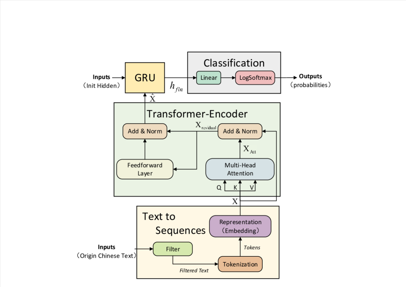
Figure 1: Transformer-Encoder-GRU

As shown in Figure 1, our model consists of four parts: text to sequence, transformer-encoder, GRU and classification. Text to sequence converts original Chinese text into vector sequence. Transformer-encoder reprocesses the original vector sequence So that each processed vector is determined by the entire input vector sequence. GRU uses the characteristics of recurrent model to process sequence features. Due to the reprocessing in the transformer-encoder, processed vector has global information, which can better deal with the problem of long sequence information loss, and this problem is the most difficult one to overcome in recurrent model. Finally, the final state of the GRU is adopted as the input of the classification to output the predicted probability.

3.1 Text To Sequence

Text to sequence maps the original Chinese text to vector sequence $X=(x_{1},x_{2},\cdots,x_{n})$, where $x_{i}\in\mathbb{R}^{d_{R}}$. n is the number of tokens and $d_{R}$ is the dimension of word representation. Text to sequence mainly consists of three parts: filter, tokenization, representation. Filter is used to deal with irregular punctuation, characters, etc. in the original Chinese text. After filtering, the tokens generated after tokenization will be shorter than before and will be fewer meaningless tokens. Specifically, the filter selectively removes most of the punctuation that does not have the ability to clause. Then tokenization convert the filtered text into a series of tokens. Here, any suitable CWS library can be used, and we use Jieba to finish CWS. Next, we use vectors to represent these tokens. Word embedding is one of the important representation methods. Representation takes these tokens as input and vector sequence $X=(x_{1},x_{2},\cdots,x_{n})$ as output. After the above processes, text to sequence converts the original Chinese text into vector sequence $X$.

3.2 Transformer-Encoder

Transformer-encoder takes $X$ from text to sequence as input and generates output $\hat{X}=(\hat{x}_{1},\hat{x}_{2},\cdots,\hat{x}_{n})$. As shown in Figure 1, transform-encoder is mainly divided into multi-head self-attention and feedforward network.

Attention mechanism has become one of the most effective methods to capture global information attentionInMulTask ; attentionInNLP ; vaswani2017Transformer . Multi-head attention is based on scaled dot-product attention proposed by Vaswani et al. vaswani2017Transformer . Multi-head attention is shown in the following equations:

$$\begin{split}&MultiHead(Q,K,V)=concat(Att_{1},Att_{2},...,Att_{n})\\ &where\ \ Att_{i}=softmax(\frac{QK^{T}}{\sqrt{d_{k}}})V\end{split}$$ (1)

where $Q,K,V$ represent query, keys and values respectively which they are all input matrices, $d_{k}$ represents the dimension of the keys, $n$ equals to the number of heads, and we set $n=2$ in our model. Especially when $Q,K,V$ are the same, it is called self-attention. Here we use the output $X$ from text to sequence as $Q,K,V$, and then output $X_{Att}$. Then we use residual connection and feedforward network in the following:

$$\begin{split}&X_{Att}=MultiHead(X,X,X)\\ &X_{residual}=norm(X_{Att}+X)\\ &\hat{X}=norm(X_{residual}+\text{FFN}(X_{residual}))\end{split}$$ (2)

where $norm$ is normalization layer, FFN consists of two linear transformations with a ReLU:

$$\text{FFN}(X_{residual})=Linear(\max(0,Linear(X_{residual})))$$ (3)

where the dimension of inner-layer is 2048 and other details of transformer-encoder are mentioned in vaswani2017Transformer .

Finally, transformer-encoder transfers $X=(x_{1},x_{2},\cdots,x_{n})$ to $\hat{X}=(\hat{x}_{1},\hat{x}_{2},\cdots,\hat{x}_{n})$, where $\hat{x_{i}}$ is determined by the entire input $X$.

3.3 GRU

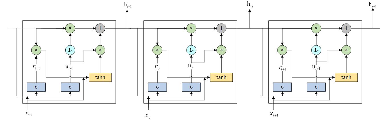
Figure 2: GRU

GRU is one of the variants of RNN, which improved from the LSTM. It performs similarly to LSTM, but is computationally cheaper. As shown in Figure 2. For any input state $x_{t}$ and the hidden state $h_{t-1}$ generated by the previous sequence:

$$\begin{split}&u_{t}=sigmoid(x_{t}W_{z}+h_{t-1}U_{z})\\ &r_{t}=sigmoid(x_{t}W_{r}+h_{t-1}U_{r})\\ &h_{t}=(1-u_{t})h_{t-1}+u_{t}*tanh(x_{t}W_{h}+(h_{t-1}\cdot r_{t})U_{h})\end{split}$$ (4)

where $r_{t}$ is the reset gate, $u_{t}$ is the update gate,$W_{z,r,h}$ and $U_{z,r,h}$ are the weight matrices that need to be trained.

Here we take $\hat{X}$ from transformer-encoder as input of GRU to generate the state sequence $(h_{1},h_{2},\cdots,h_{n})$. We use the final state $h_{n}$ as the output of GRU, and then use the classification to implement CSA. The classification here is simply composed of a linear layer and logsoftmax.

4 Experimental

In this section, we compare our method with the state-of-the-art frameworks (Including various recurrent neural networks and recurrent neural networks with attention) on three datasets for CSA tasks, including DMCS_V2 4.1, YF_DianPing 4.2 and Online_shopping_10 cats 4.3 datasets. We also conduct ablation study to research the performances of T-E-GRU.

4.1 DMCS_V2

Dataset. Douban movie short comments dataset V2 (DMSC_V2) comes from the Kaggle competition. It collects user reviews, ratings, and likes of movies on Douban (a platform for Chinese film lovers). This dataset collected short user reviews of 28 popular movies, with a total of more than 2 million comments. We label 1, 2-star reviews as “negative reviews” and 4,5-star reviews as “positive reviews” (3-star reviews are ignored because of its vague sentimentality). In the experiments we randomly selected 700,000 comments data including 350,000 positive samples and 350,000 negative samples. We divide them into three parts, 480,000 for the training set, 120,000 for the validation set, and 100,000 for the test set.

Data preprocessing. Firstly, we need to deal with the punctuation in the text data. Since the use of punctuation marks in most short film reviews is not standardized, and some punctuation has less semantic information, we retain some punctuation with clause ability, such as comma, full stops, question marks, semicolons, etc. and deleted others. Our focus is not to discuss CWS model or the necessity of CWS in deep learning models, so we use open source library Jieba developed by Baidu engineer Sun Junyi. After word segmentation, we pad and truncate the tokens for batch processing. In addition, we use pre-trained word embedding to convert words into vectors, which was trained by Li S, Zhao Z, Hu R, et al. preTrainEmbedding by using skip-gram with negative sample method based on Zhihu Q&A preTrainEmbedding . It contains 260,000 used high-frequency words, which can cover 93.98% of the words in train set. The dimension of the word vector is 300. DMCS_V2 is a short movies comments dataset. After tokenization, 99.8% of samples’ tokens are less than 100. So we align the input sequence to 100 by padding and truncating it at the front of it. For word representation, we use 200,000 high-frequency words in the pre-trained word embedding model, which can cover 93.86% of the word needed in there.

Train Details. In the experiments of RNN, LSTM and GRU, we use negative log-likelihood (NLL) loss function, set the batch size and the hidden size to 128 and 256 respectively, adopt Stochastic Gradient Descent (SGD) optimizer with learning rate of 0.002 for 100 epochs, and decay the learning rate by 0.5 every 50 epochs. We use the same settings for the bi-directional recurrent model, and the model combined with attention mechanism and recurrent models as mentioned in before, except that the hidden layer in a single direction is set to 128, and set the learning rate to 0.01. Finally, we also use the same setting on our T-E-GRU, and set the dropout of transformer-encoder to 0.3.

Results and Analysis.

Table 1: The performance of various models on the DMCS_V2

Method	Accuracy	F1	Test Time(ms)
RNN RNN-first	88.80%	88.77%	0.8483
LSTM hochreiter1997LSTM	88.41%	88.28%	2.0053
GRU cho2014learningGRU	88.70%	88.80%	1.9884
Bi-RNN	88.30%	88.30%	1.4551
Bi-LSTM	87.95%	88.02%	3.8016
Bi-GRU	88.00%	88.80%	1.4989
RNN-Attention	88.50%	88.34%	1.2503
LSTM-Attention	89.43%	89.32%	2.3592
GRU-Attention	88.08%	88.27%	2.3599
Attention-RNN	85.77%	86.09%	1.2624
Attention-LSTM	85.67%	85.55%	2.4111
Attention-GRU	84.68%	84.32%	2.3835
BiRNN-Attention	88.64%	88.50%	1.8544
BiLSTM-Attention	88.45%	88.48%	4.3638
BiGRU-Attention	88.18%	87.60%	1.9140
T-E-GRU	90.09%	90.07%	2.6987

The performance of the above models on the test set is shown in Table 1. We use accuracy and F1 as the criteria:

$$\begin{split}&Acc=\frac{TP+TN}{TP+TN+FP+FN}\\ &F1=\frac{2\times TP}{2\times TP+FP+FN}\end{split}$$ (5)

where TP, TN, FP and FN represent true positive, true negative, false positive, and false negative respectively. Test Time denotes the time required for trained model to test a comment. As shown in Table 1, the accuracy and F1 of the Bi-directional recurrent model are 0.1%$\sim$1% lower than recurrent model on DMSC_V2. The best recurrent model is simple RNN, and its accuracy and F1 have reached 88.8% and 89.0% respectively. At the same time, simple RNN also has a good performance in time with 0.8483ms. After introducing attention, the accuracy, F1 of various recurrent model have not improved much, and it also slow down the testing of the model. In addition, the improvement is only effective when the attention layer is after the recurrent layer, and the others have a slight decrease. The best recurrent model with attention is LSTM-Attention, its accuracy and F1 are 89.43% and 89.32%, which is about 0.5% improvement compared to the best recurrent model. However, compared with LSTM-Attention, T-E-GRU has an improvement of about 0.1%. In other word, T-E-GRU is the best in experimental model, with 90.09% accuracy and 90.07% F1. The drawback is that T-E—GRU costs 6% more test time than LSTM-Attention.

In general, we can find on DMSC_V2:

1. The simple RNN got the best performance in recurrent models.

2. LSTM-Attention is the best when recurrent model is combined with attention,but it also leads to more time cost.

3. T-E-GRU achieved the best performance in the models of mentioned above, with 90.09% accuracy and 90.07% F1. And the time required for model testing is very similar to LSTM-Attention.

4.2 YF_DianPing Dataset

Dataset. YF_DianPing DianpingData is customer reviews of restaurant, which has more characters and more complicated than DMSC_V2. It contains the user reviews crawled from a famous Chinese online review webset DianPing.com, including the 3,605,300 reviews of 510,071 users. After eliminating the NaN data, we randomly selected 80000 1-points reviews as positive samples, and 80,000 1-points reviews as negative samples. We divide them into two parts, 80% are used as the training set and 20% are used as the validation set. Then we obtained the test set by taking 30,000 4-points reviews as positive samples and 30,000 2-points reviews with as negative samples.

Data preprocessing. The processing of punctuation, CWS, the padding/ truncating and pre-trained word embedding model are the same as Section 4.1. After tokenization, the longest sample has 1386 tokens and 96.2% of the samples’ tokens are less than 400. So we align the input sequence to 400 by using the same method as in Section 4.1. For word representation, we use 150,000 high-frequency words, which covering 86.0% of the words in the training set. Due to the complexity of the words used in the data set, using of 260,000 high-frequency words only covers 86.5%, so it is more appropriate to use 150,000 high-frequency.

Train Details. On YF_DianPing Dataset, we did the same experiment and only modified the dataset. The various hyperparameters, loss functions, optimizers, etc. of each model are the same as Section 4.1.

Results and Analysis

Table 2: The performance of various models on the YF_DianPing

Method	Accuracy	F1	Test Time(ms)
RNN RNN-first	87.95%	88.38%	3.0484
LSTM hochreiter1997LSTM	88.40%	88.91%	7.4615
GRU cho2014learningGRU	88.83%	89.44%	7.5326
Bi-RNN	89.23%	89.51%	5.5511
Bi-LSTM	87.90%	87.50%	14.6120
Bi-GRU	89.55%	89.94%	5.3284
RNN-Attention	88.92%	89.46%	3.6268
LSTM-Attention	90.45%	90.81%	7.8170
GRU-Attention	88.55%	89.07%	7.7112
Attention-RNN	87.29%	88.12%	3.2191
Attention-LSTM	87.92%	88.54%	8.2530
Attention-GRU	88.06%	88.64%	8.1179
BiRNN-Attention	89.54%	89.86%	5.6455
BiLSTM-Attention	87.70%	88.20%	15.5177
BiGRU-Attention	88.88%	89.36%	8.6010
T-E-GRU	90.76%	90.98%	8.0009

The results of various models on the DianPing test set are shown in Table 2. The test set uses 2 points and 4 points review data, while the training set uses 1 point and 5 points review data, so there may be more ambiguous texts in the test set, resulting in poor performances. On this test set, Bi-GRU has the best performance in recurrent model, with accuracy and F1 reaching 89.55% and 89.94% respectively. Compared with the best-performing model RNN in Douban data, Bi-GRU has an improvement of about 3% on both metrics. LSTM-Attention achieves the best performances in attention-based recurrent model with 90.45% accuracy and 90.81% F1. T-E-GRU is slightly better than LSTM-Attention in both F1 and accuracy. Although not much improvement, T-E-GRU still achieved the best performance among all tested models with 90.76% accuracy and 90.98% F1. Similar to the results on Doublan, T-E-GRU still takes about 2% more test time than LSTM-Attention on this dataset.

In general, We can find:

1. RNN had a good performance on Douban before, in YF_DianPing it did not achieve good performance due to the longer tokens. The Bi-GRU has achieved the best performance in recurrent model.

2. LSTM-Attention is still the best performance in recurrent model with attention.

3. Although not much improvement, T-E-GRU still achieved the best performance among all tested models with 90.76% accuracy and 90.98% F1. This also shows that T-E-GRU can still perform well compared to other models in the face of a more complex test set than training set. And its test time is close to LSTM-Attention.

4.3 Online_shopping_10 cats Dataset

Dataset. This dataset comes from various Chinese E-commerce platforms, with a total of more than 60,000 comment data, including 30,000 positive and negative comments. We ignored their category tags and only used sentimental tags. We divide them into training set, validation set, and test set according to the ratio of 6:1:3. This dataset is smaller than the previous two datasets, and we use it to test the performance of our model on small-scale datasets.

Data preprocessing. Compared with the previous two datasets, it is a small-scale moderate-length dataset. After tokenization, the longest sample has 1502 tokens and 99.0% of the samples’ tokens are less than 200. So we align the input sequence to 200. For word representation, we use 200,000 high-frequency words, which can cover 94.9% of the word needed in the training set. Using all words in pre-trained word embedding model is only about 0.2% improvement.

Train Details. In the experiments of Online_shopping_10 cats dataset, the various hyperparameters, loss functions, optimizers, etc. of each model are the same as Section 4.1. However, since the size of this data set is small, many models use 100 epochs can not complete the training. To solve this, we double the initial learning rate and set the training epochs to 300. The performances of each model are shown in Table 3, where 300 epochs of training are marked after the model name.

Results and Analysis.

Table 3: The performance of various models on the Online_Shopping

Method	Accuracy	F1	Test Time(ms)
RNN	89.68%	89.93%	1.5092
LSTM	90.21%	90.06%	3.7045
GRU	90.08%	90.36%	3.7701
Bi-RNN	90.10%	90.07%	2.6567
Bi-LSTM	90.10%	90.10%	7.1392
Bi-GRU	90.34%	90.13%	2.8293
RNN-Attention	90.07%	90.10%	1.9176
LSTM-Attention	91.86%	91.76%	4.0548
GRU-Attention-300	90.93%	90.96%	3.9876
Attention-RNN	90.68%	90.72%	1.8351
Attention-LSTM-300	90.91%	90.91%	4.1661
Attention-GRU-300	89.56%	89.65%	4.1363
BiRNN-Attention-300	92.32%	92.38%	3.0296
BiLSTM-Attention-300	90.28%	90.16%	7.7145
BiGRU-Attention-300	91.09%	91.05%	3.2287
T-E-GRU	92.92%	93.05%	4.3890

The results of various models on the Online_shopping_10 cats test set are shown in Table 3. On this test set, various recurrent models have similar performance. The accuracy and F1 of recurrent models are around 90% and 90%. BiRNN-Attention has the best performance in recurrent model with attention, with accuracy and F1 reaching 92.32% and 92.38% respectively. Compared with the recurrent model, BiRNN-Attention has an improvement of about 2%. In contrast, LSTM-Attenion, which performed well before, was defeated on this data set. Compared with BiRNN-Attention, T-E-GRU has about 0.6% and 1% improvement in accuracy and F1 respectively, and it takes 40% more in test time.

In general, we can find:

1. On this data set, Bi-GRU still achieved the best performance in recurrent model with 90.34% accuracy and 90.13% F1. But compared to other recurrent models, the improvement of Bi-GRU is ambiguous.

2. BiRNN-Attention has achieved the best results in recurrent model with attention. Compared with recurrent model, BiRNN-Attention has about 2% improvement in accuracy and F1.

3. T-E-GRU still gains the best accuracy and F1, which are 92.92% and 93.05% respectively. And it only takes 40% more time than BiGRU-Attention.

4.4 Ablation Study

We conducted ablation experiments to better understand the contributions and the hyperparameter setting of T-E-GRU. We trained the network and tested it on the DMSC_V2, YF_DianPing and Online_shopping datasets.

4.4.1 Replacing GRU with other recurrent layer

Table 4: The performance of replacing GRU with other recurrent layers

Dataset	Method	Accuracy	F1	Test Time(ms)
DMSC_V2	T-E-RNN	89.25%	89.30%	1.5390
	T-E-LSTM	89.75%	89.88%	2.9321
	T-E-BiRNN	89.26%	89.30%	2.1434
	T-E-BiLSTM	89.81%	89.74%	4.7107
	T-E-BiGRU	89.77%	89.85%	2.2185
	T-E-GRU	90.09%	90.07%	2.6987
YF_DianPing	T-E-RNN	88.91%	89.42%	3.4685
	T-E-LSTM	90.25%	90.70%	8.0919
	T-E-BiRNN	88.94%	89.40%	5.9280
	T-E-BiLSTM	90.63%	90.92%	15.4538
	T-E-BiGRU	90.73%	90.89%	6.3677
	T-E-GRU	90.76%	90.98%	8.0009
Online_shopping	T-E-RNN	91.16%	91.01%	2.1586
	T-E-LSTM	92.43%	92.59%	4.4119
	T-E-BiRNN	91.40%	91.49%	3.3178
	T-E-BiLSTM	92.41%	92.47%	8.2653
	T-E-BiGRU	92.38%	92.60%	3.3085
	T-E-GRU-300	92.92%	93.05%	4.3890

In this section, we tried replacing GRU with other recurrent models (RNN, LSTM). The experimental results are shown in Table 4. On DMSC_V2, T-E-GRU has achieved the best performance compared to other models, but it has only a slight improvement in accuracy and F1. On YF_DianPing, T-E-GRU only has less than 1% improvement in accuracy, F1 than other models. T-E-GRU is still the best accuracy and F1, which are 90.76% and 90.98% respectively. On Online_shopping, T-E-GRU still obtain the best accuracy and F1, In general, GRU is more suitable for combining with transformer-encoder.The multiple of the time spent is usually positively correlated with the number of tokens.

4.4.2 Adjustment of hyperparameters in T-E-GRU

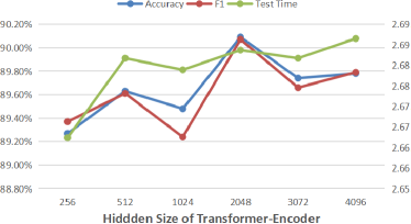
(a) DMSC_V2.

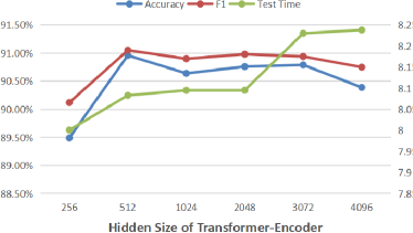
(b) YF_DianPing

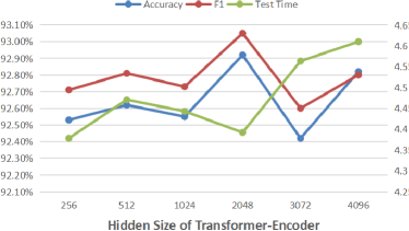
(c) Online_shopping_10 cats Dataset

Figure 3: Hidden size of Transformer-Encoder

Firstly, we tried to adjust the hidden size of the transformer-encoder. The results on three datasets mentioned in Section 4.1, 4.2, 4.3 are shown in Figure 3. The accuracy, F1, and Test Time are introduced in Section 4.1. From the results, we find that the different hidden sizes of transformer-encoder have little effect on Test Time, mostly less than 0.5(ms). For accuracy and F1, DMSC_V2 and Online_shopping have the best performance in 2048, while 2048 and 3072 on YF_DianPing have very similar performance.

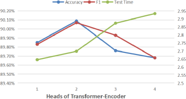
(a) DMSC_V2.

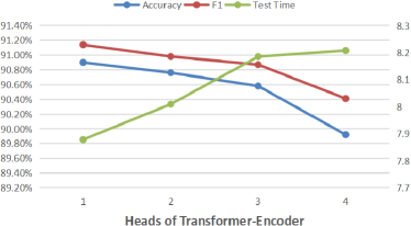
(b) YF_DianPing

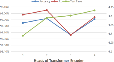
(c) Online_shopping_10 cats Dataset

Figure 4: Heads of Transformer-Encoder

Then we adjusted the number of heads in transformer-encoder. On the same datasets, the experiment results are shown in Figure 4. In fact, the number of heads from 1 to 4 has a less than 0.5(ms) effect on Test Time, and it is very slight. On DMSC_V2 and Online_shopping, the number of heads 2 can achieve the best accuracy and F1. On YF_DianPing, the number of heads 1 and 2 are similar in accuracy and F1.

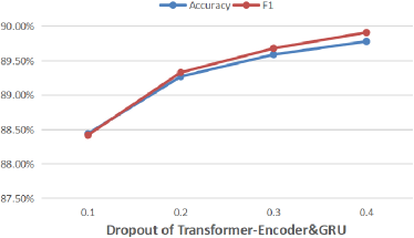
(a) DMSC_V2.

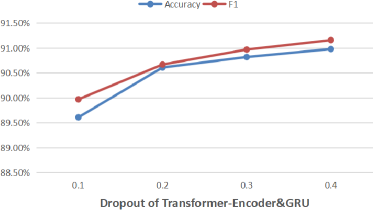
(b) YF_DianPing

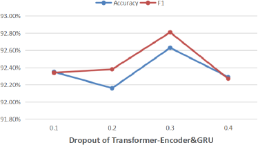
(c) Online_shopping_10 cats Dataset

Figure 5: Dropout of Transformer-Encoder & GRU

Finally, we adjusted the dropout of transformer-encoder and GRU on the same datasets. Since dropout does not affect the complexity of the model, we removed Test Time, and the result is shown in Figure 5. As the result shows, on DMSC_V2 and YF_DianPing, dropout of 0.4 is the best in accuracy and F1, while on Online_shopping, 0.3 is the best.

In general, we can find:

1. GRU is more suitable for combination with transformer-ecoder than LSTM and RNN.

2. For T-E-GRU, adjusting the hidden size of transformer-encoder, heads of transformer-encoder and dropout has little effect on Test Time, while the accuracy and F1 are different depending on the datasets.

5 Conclusion

On the three real Chinese review datasets which have not been strictly cleaned, we have retained punctuation with the ability to clauses as preprocessing. Then We compared our proposed T-E-GRU with various recurrent model and recurrent model with attention. On the test set, compared to the best performance in other models, T-E-GRU has 1% improvement in accuracy and F1.

References

- [1] Dzmitry Bahdanau, Kyunghyun Cho, and Yoshua Bengio. Neural machine translation by jointly learning to align and translate. arXiv preprint arXiv:1409.0473, 2014.
- [2] Yoshua Bengio, Réjean Ducharme, Pascal Vincent, and Christian Janvin. A neural probabilistic language model. The journal of machine learning research, 3:1137–1155, 2003.
- [3] Yoshua Bengio, Patrice Simard, and Paolo Frasconi. Learning long-term dependencies with gradient descent is difficult. IEEE transactions on neural networks, 5(2):157–166, 1994.
- [4] Liang Bin, Liu Quan, Xu Jin, Zhou Qian, and Zhang Peng. Aspect-based sentiment analysis based on multi-attention cnn. Journal of Computer Research and Development, 54(8):1724, 2017.
- [5] William B Cavnar, John M Trenkle, et al. N-gram-based text categorization. In Proceedings of SDAIR-94, 3rd annual symposium on document analysis and information retrieval, volume 161175. Citeseer, 1994.
- [6] Peng Chen, Zhongqian Sun, Lidong Bing, and Wei Yang. Recurrent attention network on memory for aspect sentiment analysis. In Proceedings of the 2017 conference on empirical methods in natural language processing, pages 452–461, 2017.
- [7] Xinchi Chen, Xipeng Qiu, Chenxi Zhu, Pengfei Liu, and Xuan-Jing Huang. Long short-term memory neural networks for chinese word segmentation. In Proceedings of the 2015 Conference on Empirical Methods in Natural Language Processing, pages 1197–1206, 2015.
- [8] Jianpeng Cheng, Li Dong, and Mirella Lapata. Long short-term memory-networks for machine reading. arXiv preprint arXiv:1601.06733, 2016.
- [9] Kyunghyun Cho, Bart Van Merriënboer, Caglar Gulcehre, Dzmitry Bahdanau, Fethi Bougares, Holger Schwenk, and Yoshua Bengio. Learning phrase representations using rnn encoder-decoder for statistical machine translation. arXiv preprint arXiv:1406.1078, 2014.
- [10] Jacob Devlin, Ming-Wei Chang, Kenton Lee, and Kristina Toutanova. Bert: Pre-training of deep bidirectional transformers for language understanding. arXiv preprint arXiv:1810.04805, 2018.
- [11] Xiaowen Ding, Bing Liu, and Philip S Yu. A holistic lexicon-based approach to opinion mining. In Proceedings of the 2008 international conference on web search and data mining, pages 231–240, 2008.
- [12] Jeffrey L Elman. Finding structure in time. Cognitive science, 14(2):179–211, 1990.
- [13] Ronen Feldman. Techniques and applications for sentiment analysis. Communications of the ACM, 56(4):82–89, 2013.
- [14] Jie Gao. Chinese sentiment classification model based on pre-trained bert. In 2021 2nd International Conference on Computers, Information Processing and Advanced Education, pages 1296–1300, 2021.
- [15] Sepp Hochreiter and Jürgen Schmidhuber. Long short-term memory. Neural computation, 9(8):1735–1780, 1997.
- [16] Dichao Hu. An introductory survey on attention mechanisms in nlp problems. In Proceedings of SAI Intelligent Systems Conference, pages 432–448. Springer, 2019.
- [17] Changning Huang and Hai Zhao. Chinese word segmentation: A decade review. Journal of Chinese Information Processing, 21(3):8–20, 2007.
- [18] MI Jordan. Serial order: a parallel distributed processing approach. technical report, june 1985-march 1986. Technical report, California Univ., San Diego, La Jolla (USA). Inst. for Cognitive Science, 1986.
- [19] John Lafferty, Andrew McCallum, and Fernando CN Pereira. Conditional random fields: Probabilistic models for segmenting and labeling sequence data. 2001.
- [20] Shen Li, Zhe Zhao, Renfen Hu, Wensi Li, Tao Liu, and Xiaoyong Du. Analogical reasoning on chinese morphological and semantic relations. arXiv preprint arXiv:1805.06504, 2018.
- [21] Xiaoya Li, Yuxian Meng, Xiaofei Sun, Qinghong Han, Arianna Yuan, and Jiwei Li. Is word segmentation necessary for deep learning of chinese representations? arXiv preprint arXiv:1905.05526, 2019.
- [22] Jun Liang, Yumei Chai, Huibin Yuan, ML Gao, and Hongying Zan. Polarity shifting and lstm based recursive networks for sentiment analysis. Journal of Chinese Information Processing, 29(5):152–159, 2015.
- [23] Shiwei Liu, Decebal Constantin Mocanu, Yulong Pei, and Mykola Pechenizkiy. Selfish sparse rnn training. arXiv preprint arXiv:2101.09048, 2021.
- [24] Tomas Mikolov, Ilya Sutskever, Kai Chen, Greg Corrado, and Jeffrey Dean. Distributed representations of words and phrases and their compositionality. arXiv preprint arXiv:1310.4546, 2013.
- [25] Tomáš Mikolov, Wen-tau Yih, and Geoffrey Zweig. Linguistic regularities in continuous space word representations. In Proceedings of the 2013 conference of the north american chapter of the association for computational linguistics: Human language technologies, pages 746–751, 2013.
- [26] Volodymyr Mnih, Nicolas Heess, Alex Graves, and Koray Kavukcuoglu. Recurrent models of visual attention. arXiv preprint arXiv:1406.6247, 2014.
- [27] Jeffrey Pennington, Richard Socher, and Christopher D Manning. Glove: Global vectors for word representation. In Proceedings of the 2014 conference on empirical methods in natural language processing (EMNLP), pages 1532–1543, 2014.
- [28] Matthew E Peters, Mark Neumann, Mohit Iyyer, Matt Gardner, Christopher Clark, Kenton Lee, and Luke Zettlemoyer. Deep contextualized word representations. arXiv preprint arXiv:1802.05365, 2018.
- [29] Lawrence Rabiner and Biinghwang Juang. An introduction to hidden markov models. ieee assp magazine, 3(1):4–16, 1986.
- [30] Alec Radford, Karthik Narasimhan, Tim Salimans, and Ilya Sutskever. Improving language understanding by generative pre-training. 2018.
- [31] David E Rumelhart, Geoffrey E Hinton, and Ronald J Williams. Learning internal representations by error propagation. Technical report, California Univ San Diego La Jolla Inst for Cognitive Science, 1985.
- [32] Xiaoming Shi and Ran Lu. Attention-based bidirectional hierarchical lstm networks for text semantic classification. In 2019 10th International Conference on Information Technology in Medicine and Education (ITME), pages 618–622. IEEE, 2019.
- [33] Fuhong Tang and Kwankamol Nongpong. Chinese sentiment analysis based on lightweight character-level bert. In 2021 13th International Conference on Knowledge and Smart Technology (KST), pages 27–32. IEEE, 2021.
- [34] Shikhar Vashishth, Shyam Upadhyay, Gaurav Singh Tomar, and Manaal Faruqui. Attention interpretability across nlp tasks. arXiv preprint arXiv:1909.11218, 2019.
- [35] Ashish Vaswani, Noam Shazeer, Niki Parmar, Jakob Uszkoreit, Llion Jones, Aidan N Gomez, Lukasz Kaiser, and Illia Polosukhin. Attention is all you need. arXiv preprint arXiv:1706.03762, 2017.
- [36] Shitao Wang, Jiangfeng Li, and Defeng Hu. Bigru-multi-head self-attention network for chinese sentiment classification. In Journal of Physics: Conference Series, volume 1827, page 012169. IOP Publishing, 2021.
- [37] Zheng Xiao and PiJun Liang. Chinese sentiment analysis using bidirectional lstm with word embedding. In International Conference on Cloud Computing and Security, pages 601–610. Springer, 2016.
- [38] Yushi Yao and Zheng Huang. Bi-directional lstm recurrent neural network for chinese word segmentation. In International Conference on Neural Information Processing, pages 345–353. Springer, 2016.
- [39] Lei Zhang, Shuai Wang, and Bing Liu. Deep learning for sentiment analysis: A survey. Wiley Interdisciplinary Reviews: Data Mining and Knowledge Discovery, 8(4):e1253, 2018.
- [40] Yongfeng Zhang, Min Zhang, Yiqun Liu, Shaoping Ma, and Shi Feng. Localized matrix factorization for recommendation based on matrix block diagonal forms. In Proceedings of the 22nd international conference on World Wide Web, pages 1511–1520, 2013.
- [41] Haoyi Zhou, Shanghang Zhang, Jieqi Peng, Shuai Zhang, Jianxin Li, Hui Xiong, and Wancai Zhang. Informer: Beyond efficient transformer for long sequence time-series forecasting. arXiv preprint arXiv:2012.07436, 2020.
- [42] Zhengshuai Zhu, Yanquan Zhou, and Shuhao Xu. Transformer based chinese sentiment classification. In Proceedings of the 2019 2nd International Conference on Computational Intelligence and Intelligent Systems, pages 51–56, 2019.
- [43] Huang Zou, Xinhua Tang, Bin Xie, and Bing Liu. Sentiment classification using machine learning techniques with syntax features. In 2015 International Conference on Computational Science and Computational Intelligence (CSCI), pages 175–179. IEEE, 2015.