Search for Cosmological time dilation from Gamma-Ray Bursts - A 2021 status update

Abstract

We carry out a search for signatures of cosmological time dilation in the light curves of Gamma Ray Bursts (GRBs), detected by the Neil Gehrels Swift Observatory. For this purpose, we calculate two different durations ($T_{50}$ and $T_{90}$) for a sample of 247 GRBs in the fixed rest frame energy interval of 140-350 keV, similar to a previous work Zhang et al. (2013). We then carry out a power law-based regression analysis between the durations and redshifts. This search is done using both the unbinned as well as the binned data, where both the weighted mean and the geometric mean was used. For each analysis, we also calculate the intrinsic scatter to determine the tightness of the relation. We find that the weighted mean-based binned data for long GRBs and the geometric mean-based binned data is consistent with the cosmological time dilation signature, whereas the analyses using unbinned durations show a very large scatter. We also make our analysis codes and the procedure for obtaining the light curves and estimation of $T_{50}$/$T_{90}$ publicly available.

I Introduction

Gamma-ray bursts (GRBs) are short-duration single-shot transient events detected in keV-MeV energy range, and constitute one of the biggest and brightest explosions in the universe, with isotropic-equivalent energies between $10^{48}$ and $10^{55}$ ergs Kumar and Zhang (2015). GRBs have been traditionally bifurcated into two categories based on $T_{90}$ and $T_{50}$, which represent the durations over which 90% and 50% of fluence are detected, respectively Kouveliotou et al. (1993). GRBs with $T_{90}>2$ secs are known as long bursts and associated with core-collapse supernovae, whereas those with $T_{90}<2$ seconds are known as short bursts and usually associated with compact object mergers Levan et al. (2016); Piran (2004); Nakar (2007); Berger (2014). There are, however, exceptions to this broad dichotomy, and additional sub-classes of GRBs have also been identified Horváth (1998, 2002); Horváth et al. (2006, 2008); Zhang et al. (2009); Horváth et al. (2010); Bromberg et al. (2013); Kulkarni and Desai (2017); Tarnopolski (2019); Horváth et al. (2018). The smoking gun evidence for the association of short GRBs with compact binary object mergers (involving neutron stars) was, however, provided by the simultaneous detection of gravitational waves and gamma rays from GW170817/GRB170817A Abbott et al. (2017), which also enabled tests of a whole slew of modified gravity theories Boran et al. (2018).

Although GRBs were first detected in the 1970s Klebesadel et al. (1973) there were still lingering doubts as to whether GRBs are local or cosmological until the 1990s (see the contrasting viewpoints on this issue by  Paczynski (1995) versus  Lamb (1995), as of 1995.) This issue was unequivocally resolved in favour of a cosmological origin, after the first precise localization and redshift determination in 1997 from the Beppo-Sax satellite van Paradijs et al. (1997). After the launch of the Neil Gehrels Swift observatory (Swift, hereafter), a large number of GRBs with confirmed redshifts have been detected Gehrels et al. (2004).

Despite this, no smoking gun signature of cosmological time dilation has emerged in the GRB light curves ever since the earliest proposed attempts Piran (1992); Paczynski (1992), unlike the corresponding signature found in Type Ia supernovae Goldhaber et al. (2001). We note, however, that such a time dilation has also not been seen in quasar light curves, although the reasons have been attributed to other astrophysical effects which mask the cosmological time dilation signal Hawkins (2010). Before the launch of the Swift satellite, there were a few indirect pieces of evidence for cosmological time dilation in GRB light curves Norris et al. (1994); Che et al. (1997); Deng and Schaefer (1998); Lee et al. (2000); Chang (2001). The main difficulty in coming to a robust conclusion in these early studies stemmed from the uncertainty in the intrinsic GRB duration and very little statistics of GRBs with well-measured redshifts. However, even after the launch of Swift and FERMI gamma-ray space telescope, there were no smoking gun signatures of cosmological time dilation in the GRB light curves Sakamoto et al. (2011); Kocevski and Petrosian (2013); Gruber et al. (2011); Lien et al. (2016); Crawford (2018) or via indirect methods such as through the skewness of $T_{90}$ distributions Tarnopolski (2020).

The first novel attempt at measuring a robust signature of cosmological time dilation using a large sample of Swift GRBs was carried out by Zhang et al. (2013) (Z13, hereafter). Z13 pointed out that all previous studies of cosmological time dilation prior to their work were carried out from the durations in the observer frame using a fixed energy interval, usually corresponding to the energy senstivity of the detector, which was the main reason for not seeing a smoking-gun signature. To circumvent this, they calculated the durations for a sample of 139 Swift GRBs using a fixed energy interval between 140-350 keV in the GRB rest frame, followed by calculating the observed durations using $E_{obs}=E_{rest}/(1+z)$, where $E_{obs}$ and $E_{rest}$ denote the photon energy in the observer and rest frame, respectively. Z13 showed after binning the data as a function of redshift that the durations were correlated with $(1+z)$, i.e., ($T_{90}\propto(1+z)^{0.94\pm 0.26}$). This analysis was then extended by  Golkhou and Butler (2014) to 237 Swift GRBs and 57 Fermi-GBM GRBs using three independent measures of duration: $T_{90}$, $T_{50}$, and $T_{R45}$. They showed that the binned data for the Swift GRB sample is broadly consistent with cosmological time dilation.

We independently carry out the same procedure as Z13 by using the latest Swift GRB database. We then carry out a power-law based regression analysis between the durations and redshifts using both the unbinned well as binned data. We also thoroughly document the procedure for obtaining the Swift light curves for every GRB and obtain the $T_{90}$, which would benefit readers for carrying out any analysis using the GRB light curves. This manuscript is organized as follows. Our data analysis and results are presented in Sect. II. We conclude in Sect. III. Detailed documentation of the procedure to get the GRB light curves and calculate $T_{50}$/$T_{90}$ can be found in Appendix A.

II Data Analysis and Results

We construct light curves for all the GRBs detected by Swift with confirmed redshifts in the fixed rest frame energy interval between 140-350 keV (similar to Z13), and thereby determine $T_{50}$ and $T_{90}$. The full step-by step procedure to download these light curves and obtain $T_{50}$/$T_{90}$ is documented in Appendix A. We have also uploaded these codes on a github link, which can be found at the end of the manuscript. Out of all the GRBs containing redshift data present in the Swift database (around 400), we were able to determine the durations for 247 of them. A tabulated summary of these durations along with 1$\sigma$ rs in the fixed rest frame energy interval (140-350 keV) as well as the full energy range in the observer frame for all GRBs can be found in Table LABEL:Table1:Swift_GRBs.

We now describe the procedure for checking if the aforementioned GRB durations are consistent with the signature of cosmological time dilation. For this purpose, we carry out a power law-based regression analysis between the observed durations and the redshift using the following equation

$$\centering y=Ax^{B}\@add@centering$$ (1)

where $A$ and $B$ are parameters of our model (unknown before the analysis, $x$ is an input variable with $x=(1+z)$ , where $z$ is the redshift, and $y$ denotes the burst interval (either $T_{90}$ or $T_{50}$) in seconds. For cosmological time dilation, $B$ should be equal to one.

To get the best-fit parameters we maximize the likelihood as follows:

$$-2\ln L = \large{\sum_{i}}\ln 2\pi\sigma_{i}^{2}+\large{\sum_{i}}\frac{[y_{i}-Ax_{i}^{B}]^{2}}{\sigma_{i}^{2}}$$ (2)

$$\sigma_{i}^{2} = \sigma_{y_{i}}^{2}+m^{2}\sigma_{x_{i}}^{2}+\sigma_{int}^{2}$$

where $x_{i}$ is $(1+z)$ data for every GRB. Similar to our works on galaxy clusters Gopika and Desai (2020); Pradyumna et al. (2021); Bora and Desai (2021) and also Tian et al. (2020), we have added in quadrature, an unknown intrinsic scatter $\sigma_{int}$ as an additional free parameter while fitting for Eq. 1. This can be used to parameterize the tightness of the scatter in the relation. A value of $\sigma_{int}>1$ indicates that the relation has a lot of scatter and that any relation between the two variables cannot be discerned. On the other hand, a small value of scatter points to a deterministic relation between the two variables. Note that Z13 have investigated for putative correlations between the durations and redshifts using the Pearson correlation coefficient. However, the Pearson correlation coefficient does not take into account the errors in the observables. The magnitude of the intrinsic scatter would be a more robust diagnostic of the scatter.

We use the emcee MCMC routine Foreman-Mackey et al. (2013) to sample the above likelihood and obtained 68%, 90%, and 95% marginalized credible intervals on each of the parameters. We use uniform priors on all the free parameters : $0<A<50$, $-1<B<4$, $-5<\ln(\sigma_{int})<5$. In all the cases, the marginalized contours were obtained using the Corner package, and estimates are performed over parameters of the model which we are trying to optimize.

We now present our results. We carried out multiple analyses for both $T_{50}$ and $T_{90}$, using both the unbinned data as well as using the binned data. The binning was done in equal-sized redshift bins and with two different ways of averaging the data in each bin: viz. weighted mean (as in Z13) and the geometric mean (as in  Golkhou and Butler (2014)). Our results are summarized in Table 1 and  2.

• Analysis using unbinned data for all GRBs

  We first fit the $T_{50}$ and $T_{90}$ obtained for all the 247 GRBs in our sample to Eq. 1. The marginalized credible intervals for the unbinned data are given by Fig. 1 and Fig. 2 for both $T_{50}$ and $T_{90}$, respectively. As we can see, the intrinsic scatter is greater than 100%, indicating that it is difficult to discern a deterministic relation between $T_{50}$ or $T_{90}$ and the redshift. Furthermore, the power-law index $B$ is not equal to the cosmological expected value of one to within 1$\sigma$. Fig. 3 shows the plots for both the burst intervals, $T_{90}$ and $T_{50}$, along with the best-fit obtained from fitting the full unbinned data.

  

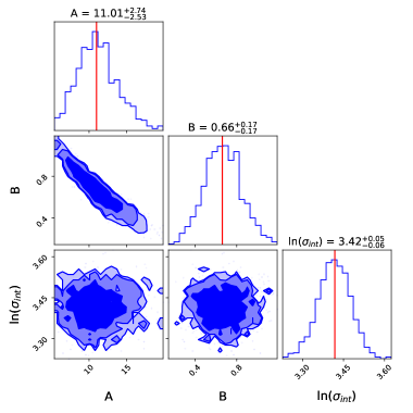
  Figure 1: Figure showing the contour plot for $T_{50}$ in the rest-frame energy range 140-350 keV, for the unbinned GRB data. The contours represent 68%, 90%, and 95% credible intervals. As we can see, the intrinsic scatter is quite high ($>$ 100%), which implies that it is hard to discern a deterministic relation between $T_{50}$ and the redshift.

  

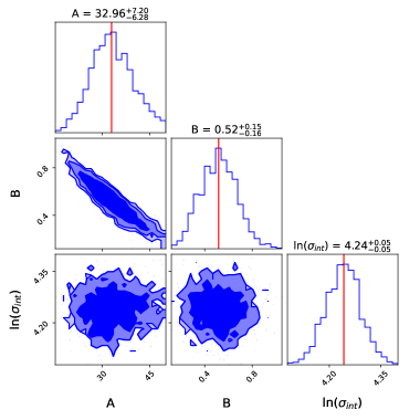
  Figure 2: Figure showing the contour plot $T_{90}$ in the rest-frame energy range 140-350 keV, for the unbinned GRB data. The contours represent 68%, 90%, and 95% credible intervals. Again, the intrinsic scatter is very high ($>$ 100%).

  

  

  Figure 3: Figure showing the relationship between the burst intervals, $T_{90}$ and $T_{50}$ in the observer frame energy range $E_{1}=140/(1+z)$ keV and $E_{2}=350/(1+z)$ keV (denoted by $T_{90}$, $T_{50}$), for the unbinned GRB data. The data points have been plotted with their respective error bars. The best fits are shown by the dashed blue lines and those are $T_{50}={\color[rgb]{0,0,0}11.01}(1+z)^{{\color[rgb]{0,0,0}0.66}}$ and $T_{90}={\color[rgb]{0,0,0}32.96}(1+z)^{{\color[rgb]{0,0,0}0.52}}$ respectively.

• Analysis using weighted-mean binned data for all GRBs

  We now re-analyze this data by binning the data into six bins with equal redshift intervals and using the error-weighted means of both the burst intervals, $T_{90}$ and $T_{50}$ in each redshift bin. The marginalized contours for $A$ and $B$ for such a binned analysis for both $T_{50}$ and $T_{90}$ can be found in Figs. 4 and 5, respectively. We find that $B$ is discrepant from the cosmological expected value of one at 1.2$\sigma$ ($T_{50}$) and 2$\sigma$ ($T_{90}$). The intrinsic scatters are approximately 75% for both $T_{50}$ and $T_{90}$. This shows that there is still no evidence for cosmological time dilation signature using the complete binned sample. The binned data along with the best fit can be found in Fig. 6.

  

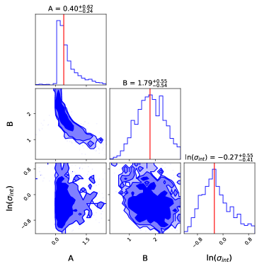
  Figure 4: Contours for $A$ and $B$ for $T_{50}$ in the rest-frame energy range 140-350 keV. The input data is the weighted mean of binned data of $T_{50}$ vs the binned redshifts (1+z). This data is then fit to Eq 1. We have shown 68%, 90%, and 95% credible intervals. The intrinsic scatter we obtain is about 76%. The value of $B$ is discrepant with the signature of cosmological time dilation at about $1.2\sigma$.

  

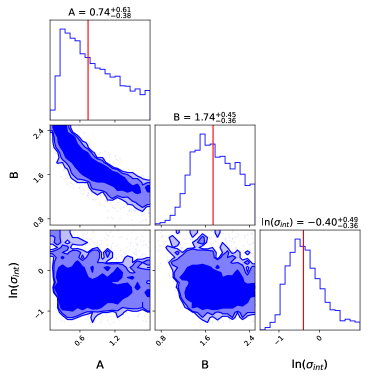
  Figure 5: Contours for $A$ and $B$ using 90% burst interval, $T_{90}$ in the rest-frame energy range 140-350 keV. Input data is the weighted mean of binned data of the $T_{90}$ vs the binned redshifts (1+z). This data is then fit to Eq. 1. We have shown 68%, 90%, and 95% credible intervals. The intrinsic scatter is equal to 76.3%. The value of $B$ is discrepant with the signature of cosmological time dilation at about $2\sigma$.

  

  

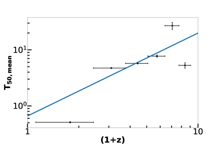
  Figure 6: Plots showing the weighted means of the burst intervals with the binned redshift data (containing 6 groups equally spaced in $z$), where the horizontal errors bars denote the redshift range in each group. The blue line curve is our best fit for the data obtained through the estimation of parameters $A$ and $B$. The best-fits shown are $T_{50}={\color[rgb]{0,0,0}0.40}(1+z)^{{\color[rgb]{0,0,0}1.79}}$ and $T_{90}={\color[rgb]{0,0,0}0.74}(1+z)^{{\color[rgb]{0,0,0}1.74}}$.

• Analysis using unbinned data for long GRBs

  Z13 and Ref. Golkhou and Butler (2014) did their analysis using only long GRBs, with $T_{90}>$ 2 secs. The reason for this exclusion of short GRBs is to have a pure sample with an intrinsically similar distribution. We now present similar results using only long GRBs with the cut of $T_{90,raw}>2$ secs. We show the marginalized contours for both $A$ and $B$, for both $T_{90}$ and $T_{50}$ in Figs. 7 and  8. Similar to the full unbinned GRB dataset, the intrinsic scatter is $>100\%$ making it impossible to discern any relation between the duration and redshift. Furthermore, the values of $B$ are not equal to one (at more than $1\sigma$) for both $T_{90}$ and $T_{50}$ Fig. 9 shows the burst intervals as a function of redshift for this subset along with the best fit.

  

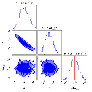
  Figure 7: Contours for $A$ and $B$ for $T_{50}$, in the rest-frame energy range 140-350 keV for long GRBs which have $T_{90,raw}$ greater than 2 secs. We have shown 68%, 90%, and 95% credible intervals. The intrinsic scatter is greater than 100%.

  

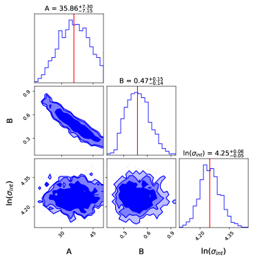
  Figure 8: Contours for $A$ and $B$ for $T_{90}$ in the rest-frame energy range 140-350 keV, for long GRBs which had a $T_{90,raw}$ greater than 2 secs. The intrinsic scatter is greater than 100%.

  

  

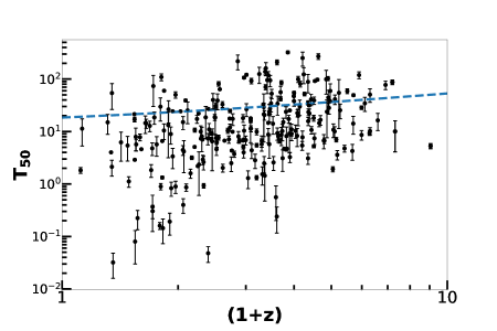
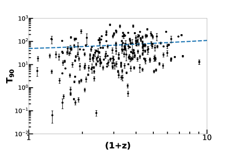
  Figure 9: Figure showing the relationship between the burst intervals, $T_{90}$ and $T_{50}$ in observer energy range (denoted by $T_{90}$, $T_{50}$), for long GRBs which had $T_{90,raw}>2$ seconds. Through curve fitting, we obtain $T_{50}={\color[rgb]{0,0,0}12.01}(1+z)^{{\color[rgb]{0,0,0}0.62}}$ and $T_{90}={\color[rgb]{0,0,0}35.86}(1+z)^{{\color[rgb]{0,0,0}0.47}}$.

• Analysis using binned data for long GRBs

  We now bin the data for long GRBs and use the weighted mean in each redshift bin. The marginalized contours for both $A$ and $B$, which are obtained by fitting the model in Eq. 1, using the binned data can be found in Figs 10 and 11. We obtain intrinsic scatters of 57% and 55% for $T_{50}$ and $T_{90}$, respectively. The values of $B$ for both the binned durations are consistent with the cosmological time dilation signature ($B=1$) to within 1$\sigma$. We show the weighted mean burst intervals for these long GRBs, with redshifts in Fig. 12, along with the best-fit.

  

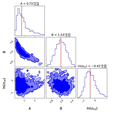
  Figure 10: Plot showing 68%, 90%, and 95% credible intervals for $A$ and $B$ for $T_{50}$ in the rest frame energy range of 140-350 keV, using the binned redshift data (containing 6 groups equally spaced in $z$), for long GRBs. The intrinsic scatter is 65.7%. The value of $B$ is consistent with a cosmological time dilation signature within 1$\sigma$.

  

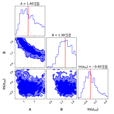
  Figure 11: Plot showing 68%, 90%, and 95% credible intervals of $A$ and $B$ for $T_{90}$ with the binned redshift data (containing 6 groups equally spaced in $z$), for long GRBs. The intrinsic scatter is equal to 67.03%. The value of $B$ is consistent with a cosmological time dilation signature within 1$\sigma$.

  

  

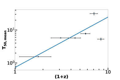
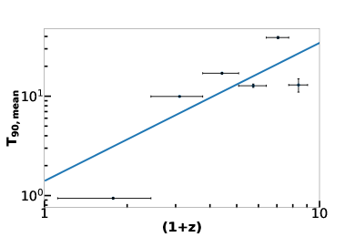
  Figure 12: Plots showing weighted means of burst intervals using only the long GRB sample, with the binned redshift data (containing 6 groups equally spaced in $z$), where the horizontal error bars denote the redshift range in each group. . The blue line is the best fit curve obtained through the estimation of parameters $A$ and $B$ (cf. Eq. 1). We obtain $T_{50}={\color[rgb]{0,0,0}0.73}(1+z)^{{\color[rgb]{0,0,0}1.53}}$ and $T_{90}={\color[rgb]{0,0,0}1.40}(1+z)^{{\color[rgb]{0,0,0}1.39}}$.

• Analysis using geometric mean binned data for all GRBs

  Ref. Golkhou and Butler (2014) pointed out that any weighted mean would be affected by outliers and one should instead use more robust estimates such as geometric mean and median. For this purpose, we also redo our search for cosmological time dilation analysis by considering the geometric mean of $T_{50}/T_{90}$ in each redshift bin. The contours for $A$ and $B$ after such a regression analysis can be found in Fig. 13 and Fig. 14 for $T_{50}$ and $T_{90}$ respectively. For $T_{50}$ the intrinsic scatter we get from this fit is $<{\color[rgb]{0,0,0}60}\%$. For $T_{90}$, the intrinsic scatter which get is $\ln(\sigma_{int})={\color[rgb]{0,0,0}1.84}^{+0.55}_{-1.33}$. Although the best-fit value of the scatter is greater than 100%, it is is consistent with 27% to within 68% c.l. Therefore, we get the tightest scatter using the geometric mean for both $T_{50}$ and $T_{90}$. The power-law exponent ($B$) we get is consistent with a cosmological signature, for $T_{50}$ and $T_{90}$ to within 1$\sigma$. The burst intervals as a function of redshift ($1+z$) are shown in Fig. 15 along with the best-fit.

The results of all our regression analyses using both the unbinned as well as binned data are summarized in Tables 1 and 2, respectively. For the unbinned analyses, the intrinsic scatter is $>100$%, which implies that we cannot draw any definitive conclusion between durations and redshifts. Our main result is that only after using the geometric mean based binned data (full sample) and weighed mean based binned data (long GRBs), we find evidence for cosmological time dilation for both these GRB durations. Among the binned analyses the data obtained using geometric mean show the smallest scatter. Therefore, we concur with Z13, that GRBs show evidence for cosmological time dilation only in a statistical sense, but not on a per-GRB basis.

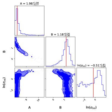
Figure 13: Contours for 68%, 90%, and 95% credible intervals $T_{50}$ in the rest frame energy range of 140-350 keV, using binned data where the geometric mean of $T_{50}$ in each bin was used. The intrinsic scatter ($\sigma_{int}$) is very low, indicating that there is a deterministic relationship between binned durations and the redshifts. The value of $B$ is consistent with the cosmological time dilation signature.

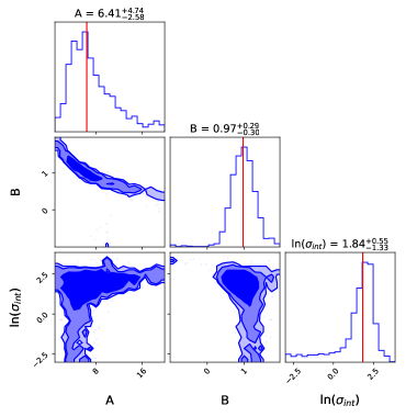
Figure 14: Contours showing 68%, 90%, and 95% credible intervals for $A$ and $B$ for $T_{90}$ in the rest frame energy range of 140-350 keV, using binned data where geometric mean of $T_{90}$ in each bin was used. Although the median intrinsic scatter is greater than 100%, it is consistent within 1$\sigma$. However, the value of $B$ is consistent with the cosmological time dilation signature to within 1$\sigma$.

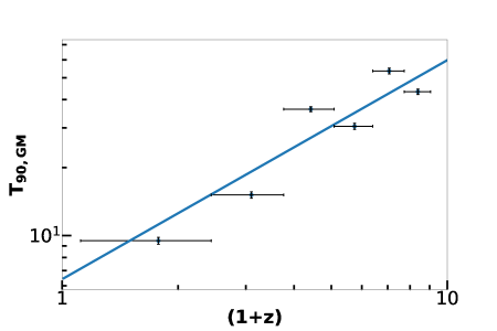
Figure 15: Plots showing geometric means of burst intervals with the binned redshift data (containing 6 groups equally spaced in z), where the horizontal error bars denote the redshift range in each group. The blue line is the best fit curve obtained through the estimation of parameters $A$ and $B$ (cf. Eq. 1). We obtain $T_{50}={\color[rgb]{0,0,0}1.98}(1+z)^{{\color[rgb]{0,0,0}1.18}}$ and $T_{90}={\color[rgb]{0,0,0}6.41}(1+z)^{{\color[rgb]{0,0,0}0.97}}$.

Table 1: Table showing a summary of best fit values of $A$, $B$, and the logarithm scatter ($\sigma_{int}$) for different kinds of analysis for unbinned GRB datasets.

Dataset	$A_{T_{50}}$	$B_{T_{50}}$	$\ln\sigma_{int,T_{90}}$	$A_{T_{90}}$	$B_{T_{90}}$	$\ln\sigma_{int,T_{90}}$
Full Sample	${\color[rgb]{0,0,0}11.01}^{+2.74}_{-2.53}$	${\color[rgb]{0,0,0}0.66}^{+0.17}_{-0.17}$	${\color[rgb]{0,0,0}3.42}^{+0.5}_{-0.6}$	${\color[rgb]{0,0,0}32.96}^{+7.82}_{-6.66}$	${\color[rgb]{0,0,0}0.52}^{+0.15}_{-0.16}$	${\color[rgb]{0,0,0}4.24}^{+0.05}_{-0.05}$
Long GRBs	${\color[rgb]{0,0,0}12.01}^{+3.14}_{-2.76}$	${\color[rgb]{0,0,0}0.62}^{+0.18}_{-0.17}$	${\color[rgb]{0,0,0}3.44}^{+0.06}_{-0.05}$	${\color[rgb]{0,0,0}35.86}^{+7.30}_{-7.15}$	${\color[rgb]{0,0,0}0.47}^{+0.15}_{-0.14}$	${\color[rgb]{0,0,0}4.25}^{+0.06}_{-0.05}$

Table 2: Table showing a summary of best fit values of $A$, $B$, and the logarithm of intrinsic scatter ($\sigma_{int}$) for different kinds of analysis for binned GRB datasets. Note that the first two rows use the weighted mean in each redshift bin. The values of $B$ are consistent with a cosmological time dilation signature for long GRBs and using geometric mean

Dataset	$A_{T_{50}}$	$B_{T_{50}}$	$\ln\sigma_{int,T_{50}}$	$A_{T_{90}}$	$B_{T_{90}}$	$\ln\sigma_{int,T_{90}}$
Full Sample	${\color[rgb]{0,0,0}0.40}^{+0.62}_{-0.24}$	${\color[rgb]{0,0,0}1.79}^{+0.55}_{-0.54}$	${\color[rgb]{0,0,0}-0.27}^{+0.55}_{-0.41}$	${\color[rgb]{0,0,0}0.74}^{+0.61}_{-0.38}$	${\color[rgb]{0,0,0}1.74}^{+0.45}_{-0.36}$	${\color[rgb]{0,0,0}-0.40}^{+0.49}_{-0.36}$
Long GRBs	${\color[rgb]{0,0,0}0.73}^{+0.75}_{-0.36}$	${\color[rgb]{0,0,0}1.53}^{+0.42}_{-0.44}$	${\color[rgb]{0,0,0}-0.42}^{+0.49}_{-0.36}$	${\color[rgb]{0,0,0}1.40}^{+0.91}_{-0.62}$	${\color[rgb]{0,0,0}1.39}^{+0.35}_{-0.31}$	${\color[rgb]{0,0,0}-0.40}^{+0.55}_{-0.39}$
Geometric mean binning	${\color[rgb]{0,0,0}1.98}^{+1.94}_{-0.77}$	${\color[rgb]{0,0,0}1.18}^{+0.26}_{-0.36}$	$<{\color[rgb]{0,0,0}-0.51}$	${\color[rgb]{0,0,0}6.41}^{+4.74}_{-2.58}$	${\color[rgb]{0,0,0}0.97}^{+0.29}_{-0.30}$	${\color[rgb]{0,0,0}1.84}^{+0.55}_{-1.33}$

II.1 Tests with rest frame durations

Similar to Z13, we carry out some additional tests to completely ascertain the redshift evolution of the intrinsic GRB duration, as found from some of the binned analyses. We calculate the rest frame $T_{90,rest}$ and from the $T_{90}$ determined earlier using $T_{90,rest}=T_{90}/(1+z)$ (and same for $T_{50}$). These rest-frame durations are shown in Fig. 16. Similar to Z13, we find a large dynamic range in the durations with median values of $3.8$ and $10$ seconds for $T_{50,rest}$ and $T_{90,rest}$, respectively, while the standard deviations are ${\color[rgb]{0,0,0}13}$ and $27$ seconds for $T_{50,rest}$ and $T_{90,rest}$ respectively. We also checked for an evolution effect of the rest frame durations with redshifts using the same procedure as done for $T_{50}$ and $T_{90}$ earlier. The best-fit values for $B$ are equal to $0.11^{+0.20}_{-0.19}$ and $-0.11^{+0.18}_{-0.17}$ for $T_{50,rest}$ and $T_{90,rest}$ respectively. Therefore, the values of $B$ are significantly different from that expected from cosmological time dilation ($B=1$). Furthermore, the logarithm of the intrinsic scatter is given by $\ln(\sigma_{int})$ is equal to $3.12^{+0.05}_{-0.05}$ and $2.17^{+0.06}_{-0.05}$ for $T_{50,rest}$ and $T_{90,rest}$ respectively, implying that the intrinsic scatter is greater than 100%. Therefore, This implies that there is no evolution of the rest frame durations, in accord with Z13’s conclusions.

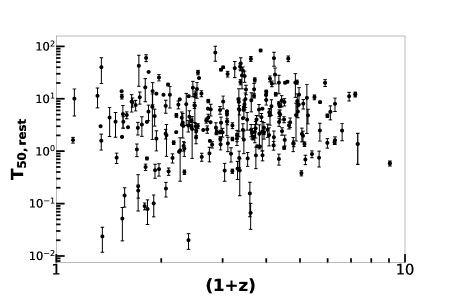
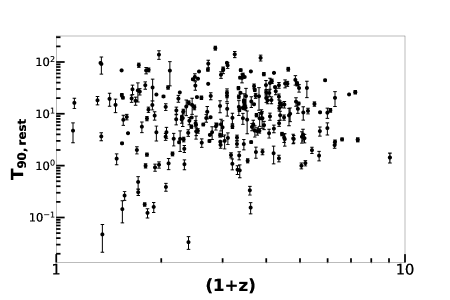
Figure 16: Plots showing the correlations between $T_{50,rest}$ and $T_{90,rest}$ in the rest frame of GRBs with the redshifts. The rest frame durations are obtained by dividing the $T_{50}/T_{90}$ tabulated in the last two columns of Table LABEL:Table1:Swift_GRBs by ($1+z$).

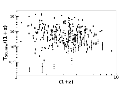
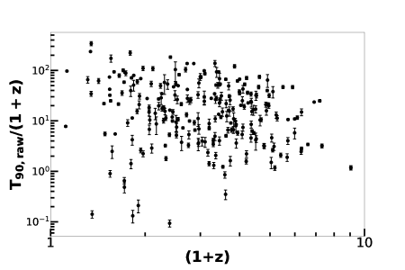
Figure 17: Plots showing the correlations between the durations in the rest frame obtained using $T_{90,raw}/({1+z})$, (where “raw” indicates data measured between 15-350 keV in the observer frame), and the redshifts. All symbols carry the usual meaning.

Finally, we check for any possible redshift evolution of rest-frame duration estimated directly from the raw durations (i.e. $T_{50,raw}/(1+z)$) as a function to redshift to independently confirm if we see a decreasing trend as found in some previous works Pélangeon et al. (2008); Kocevski and Petrosian (2013). These $T_{50,raw}/(1+z)$ and $T_{90,raw}/(1+z)$ plots can be found in Fig. 17. We find that $B$ is equal to $-0.59^{+0.21}_{-0.21}$ and ${\color[rgb]{0,0,0}-0.82}^{+0.13}_{-0.10}$ for $T_{50,raw}/(1+z)$ and $T_{90,raw}/(1+z)$, respectively. Furthermore, the logarithm of the intrinsic scatter is given by $\ln(\sigma_{int})$ which is equal to $2.91^{+0.04}_{-0.05}$ and $3.55^{+0.05}_{-0.05}$. Therefore, we again concur with Z13, that there is no evidence that the measure of rest frame duration analyzed in  Pélangeon et al. (2008); Kocevski and Petrosian (2013) shows any evolution with redshift.

III Conclusions

Even though we know for more than two decades that almost all GRBs are located at cosmological distances, the cosmological time dilation signature for GRBs has not been unequivocally demonstrated. Therefore, we independently carry out a study similar to Z13 (and also  Golkhou and Butler (2014)), using the latest updated GRB sample from the Swift satellite. We estimated $T_{50}$ and $T_{90}$ for all the GRBs in the Swift catalog, for the energy band of 140-350 keV in the rest frame. This corresponds to an energy band of $140/(1+z)$ and $350/(1+z)$ in the observer frame. These $T_{50}$ and $T_{90}$ intervals calculated for all the Swift GRBs are tabulated in Table LABEL:Table1:Swift_GRBs.

We then carry out a regression analysis between the duration and redshifts using $T_{90}$($T_{50}$) = $A(1+z)^{B}$ using both the unbinned and binned durations, where the binning was done using both a error weighted-mean as well as geometric-mean based average. We also analyzed the full sample sample as well as only the long GRB sample. For a cosmological time dilation signature, $B$ should be equal to one. Our results from all these myriad analyses are summarized in Table 1 and Table 2 for the unbinned and the binned data, respectively. We conclude that the burst intervals obtained from the geometric mean-based and weighted mean-based (long GRBs) binned analyses are consistent with the cosmological time dilation phenomenon (within $1\sigma$) for both $T_{50}$ and $T_{90}$. (cf. Table 2). The smallest intrinsic scatters are obtained using the geometric mean based binned data. The weighted mean analysis for the full sample is discrepant with respect to the cosmological time signature at 1.2$\sigma$ and 2$\sigma$ for $T_{50}$ and $T_{90}$, respectively. The unbinned analyses show intrinsic scatters $>$ 100% as well as values of $B$ significantly different from $1$, implying that no definitive conclusion between the durations and the redshifts can be inferred.

Finally, we should point out that although choosing a fixed energy frame interval may avoid the biases associated by recording different parts of the GRB intrinsic light curves, our results could still be affected by detector related selection biases. As Z13 pointed out for GRBs at higher redshifts and low SNRs, only the brightest GRBs would be detected and some of the observations could be underestimated. Secondly, the BAT effective area is energy dependent and drops sharply at energies less than 25 keV and greater than 100 keV Barthelmy et al. (2005). Another possibility, pointed out in  Golkhou and Butler (2014) is that the measured duration of a GRB could also be affected by the gradual loss of the final fast-rise exponential decay pulse tail due to the degraded signal-to-noise ratio Littlejohns et al. (2013). A detailed modeling of these effects is beyond the scope of this work. However in a future work, we shall be using the deconvolved photon fluxes for estimating $T_{90}$, which could get rid of these instrumental effects von Kienlin et al. (2020).

All the codes which are utilized in this analysis, including the batbinevt and battblocks code generators have been made publicly available and can be found at GRB Analysis Code (Github).

Appendix A Data retrieval and light curve analysis

Figure 18: A brief data processing pipeline for our analysis of the GRB samples obtained from the latest Swift catalog. The yellow boxes denote the type of products obtained and the black pointers represent the type of command used to generate those products.

We now describe the detailed step-by-step procedure for downloading the Swift light curve data and estimating $T_{50}$/$T_{90}$ for every GRB. Fig. 18 demonstrates a brief workflow of this processing pipeline, starting from raw GRB event data to the calculation of the burst intervals. We have sampled 247 of the 400 GRBs which were eligible for the analysis (containing proper redshift data). The remaining 153 GRBs could not be processed, because most of the data products (101) for the remaining GRBs did not contain any TDRSS messages, and many (52) did not have data products with enough exposure to construct detailed Bayesian blocks, needed for the estimation of durations.

We use the Burst interval data recorded by the Burst Alert Telescope (BAT) aboard Swift. The BAT instrument has two basic modes of operation: 1) scan-survey mode and 2) burst mode. These two modes reflect the two major types of data that BAT produces: hard X-ray survey data and burst positions. Most of BAT’s time is spent in waiting for a burst to occur in its FOV. Finding GRBs within BAT consists of two processes: 1) the detection of the onset of a burst by looking for increases in the event rate across the detector plan, and 2) the formation of an image of the sky using the events detected during the time interval at the beginning of the burst. Markwardt et al. (2007)

Burst Trigger Algorithm:- The burst trigger algorithm looks for detector count rate excesses that are higher than those predicted from the background and constant sources. The fluctuations in the background and the heterogeneity of the GRB time profiles are the two fundamental barriers in GRB detection. During the 90-minutes the satellite stays in Low Earth Orbit, the detector background rates can change by more than a factor of two. GRBs can last anywhere from a few milliseconds to several minutes, with anywhere from one to several dozen peaks in the emission. As a result, the triggering system must be capable of extrapolating the background and comparing it to the recorded detector count rate over a wide range of timescales and energy bands Markwardt et al. (2007).

NASA maintains an updated list of all the BAT observations at the Swift Archive Swift Team (2021). We use Web Xamin NASA (2021a), which acts as a source for downloading or saving the BAT GRB data for analysis, and Web Hera NASA (2021b) (containing the HEASOFT tools from NASA) to analyze the BAT data. HEASOFT tools provided at https://heasarc.gsfc.nasa.gov/docs/tools.html work on a Linux machine but this analysis has explicitly made use of the Web Hera interface, owing to its simplicity and minimal computational resources at the user’s end. The whole analysis can be classified into the following stages in chronological order:

• Querying for and collecting the full GRB data products at the Swift archive through the Web Xamin interface

  For this access the Web Xamin at https://heasarc.gsfc.nasa.gov/xamin/.

  We have to focus on the Query Pane for our queries.

  After we have logged in, we can obtain a table of our interest through the Table Explorer option. Now there are multiple options to get the data. We can navigate through the folders in the Table Explorer to get the whole catalogue or search a GRB by its name (ex- GRB 050126) or its coordinates in the Target for search. To get the whole catalogue, we would go to Popular Missions $\rightarrow$ Swift $\rightarrow$ Swiftbalog to obtain the data for all the GRBs observed till date. Or if we search for a particular GRB, we can type the name and then click on ‘search on all HEASARC tables’ to run our query. For example, if we want to search and download the data for GRB 050319, then when we query for the GRB, we can find all the summary tables related to the GRB.

  In this case too, out of all other tables, we just need the Swiftbalog table for getting the BAT GRB data. When we open the Swiftbalog table, we get a list of multiple data products. To figure out which event data has data products available, we need to look at the data products; they must contain a folder named as ‘TDRSS’. This would most probably be one of the long exposure files (1000-2900 seconds). This is necessary because batgrbproduct will only work on those data products that contain this folder. Then, once we have found that particular data product, we can select it and click on ‘Save to Hera’. This will save the data product to Web Hera, where we can further analyse the BAT GRB data.

• GRB Analysis in Web HERA to calculate the observer frame energy binned and full detector range light curves

  To run any command, we can use either the Command Window Terminal or the Tool Parameter. For now, we will use Tool Parameter. Type ‘batgrbproduct’ and click on Get.

  We then run batgrbproduct keeping all the parameters to their default value. We just have to specify the input folder, where the raw data lies and another folder where the output files will be stored.

  We then go to the results folder and save the file process.log to our local storage or view it elsewhere; we will then find the whole set of operations that Hera has performed using batgrbproduct command in the process.log file. We then find out the batbinevt command (used to prepare custom light curves in user-defined energy bins). A sample batbinevt command with its parameters looks like:

  ⬇

  batbinevt infile=’./00103780000-results/events/sw00103780000b_all.evt’ outfile=’./00103780000-results/lc/sw00103780000b_bb_4ms.lc’ outtype=LC timedel=0.004 timebinalg=u energybins=’15-350’ detmask=’./00103780000-results/auxil/sw00103780000b_qmap.fits’ ecol=ENERGY weighted=YES outunits=RATE clobber=yes

  Notice the parameters energybins and timedel. energybins are used to specify the energy range, and timedel is used to specify the $\Delta t$ (the time resolution in seconds). The keyword LC denotes a light curve. These light curve files have an extension .lc. For short GRBs, we use 16 ms binned light curves, while for long GRBs, we use 64 ms binned light curves (following the same convention as in  Kouveliotou et al. (1993)). This, along with the output name, can be changed to produce the required light curves.

  To calculate the light curves for obtaining the raw $T_{50}$ and $T_{90}$ (full detector energy range of 15-350 keV), we just have to copy and paste the command, without changing the energy ranges, copy the command, and run it in Hera. This will create the custom light curves that will be required for raw $T_{90}$ calculation (in the folder light curves).

• Calculation of burst intervals in rest frame and observer frame energy intervals

  For calculation of $T_{90}$ and $T_{50}$ in the rest frame energy interval of 140-350 keV, corresponding to a redshift-dependent observed energy range, we have to alter the energy bins $E_{1}=140/(1+z)$) and $E_{2}=350/(1+z)$. $E_{1}$ is the lower limit of the observed energy range, and $E_{2}$ is the upper limit. We make use of the newly created light curves to calculate estimated burst intervals ($T_{90}$ and $T_{50}$) in the different energy ranges using the Bayesian block algorithm Scargle et al. (2013).

  Now using the custom light curve file that we created, we will run the battblocks command. The input file would be the custom light curve file. We have to specify any desired name to the durfile as well as output file. Also, we have to make sure that we don’t give an optional filter, which implies that the field should be completely empty (without any text). Click on run battblocks, and this should give the $T_{90}$ and $T_{50}$ for the GRB as the final result in the Hera command console.

Table 3: Durations of 247 Swift GRBs with known redshifts evaluated in different energy bins. $T_{50}$ and $T_{90}$ are evaluated in rest frame energy interval of 140-350 keV and $T_{50,raw}$, $T_{90,raw}$ are evaluated in full detector range of BAT, 15-350 keV. We note that we have omitted GRB 130610A and GRB 160410A, as they yielded completely different T90s in the observer frame compared to the SWIFT table. Also we omitted the GRBs 150403A, 180205A and 190106A because their data products could not be found on NASA’s Swift database anymore.

GRB Name	Obs ID	z	$\mathbf{T_{90,raw}}$(s)	$\mathbf{T_{50,raw}}$(s)	$\mathbf{E^{*}_{1}}$(keV)	$\mathbf{E^{*}_{2}}$(keV)	$\mathbf{T_{90}}$(s)	$\mathbf{T_{50}}$(s)
050126	103780	1.29	$23.248\pm 2.53$	$12.432\pm 2.036$	61.14	152.84	$17.808\pm 2.771$	$10\pm 2.815$
050315	111063	1.949	$97.248\pm 14.637$	$24.976\pm 1.471$	47.47	118.68	$41.744\pm 10.809$	$18\pm 3.065$
050318	111529	1.44	$29.056\pm 0.472$	$15.344\pm 10.616$	57.38	143.44	$13.776\pm 1.018$	$7.216\pm 0.588$
050319	111622	3.24	$153.072\pm 11.31$	$124.304\pm 4.228$	33.02	82.55	$139.184\pm 6.598$	$122.784\pm 41.306$
050401	113120	2.9	$33.12\pm 1.037$	$25.792\pm 0.588$	35.90	89.74	$32.032\pm 0.77$	$25.232\pm 0.497$
050505	117504	4.27	$59.53\pm 7.108$	$26.992\pm 6.363$	26.57	66.41	$59.928\pm 7.541$	$25.408\pm 7.939$
050525A	130088	0.606	$8.832\pm 0.081$	$5.232\pm 0.0226$	87.17	217.93	$6.784\pm 0.136$	$4.608\pm 0.086$
050730	148225	3.968	$157.584\pm 14.77$	$68.352\pm 10.465$	28.18	70.45	$155.904\pm 25.613$	$59.472\pm 21.642$
050802	148646	1.52	$18.928\pm 3.494$	$8.16\pm 1.765$	55.56	138.89	$11.536\pm 1.981$	$6.208\pm 1.216$
050803	148833	0.422	$88.176\pm 9.982$	$39.392\pm 6.757$	98.45	246.13	$27.632\pm 7.789$	$6.224\pm 3.507$
050814	150314	5.3	$94.208\pm 14.575$	$42.256\pm 7.78$	22.22	55.56	$127.936\pm 40.738$	$50.544\pm 14.466$
050820A	151207	2.6147	$241.36\pm 12.277$	$220.56\pm 3.117$	38.73	96.83	$237.52\pm 4.766$	${\color[rgb]{0,0,0}229.298}\pm{\color[rgb]{0,0,0}22.092}$
050904	153514	6.2	$179.5\pm 10.3$	$85.4\pm 7.6$	19.44	48.61	$187.744\pm 14.269$	$87.216\pm 8.845$
050908	154112	3.35	$19.9\pm 3.5$	$6.7\pm 2$	32.18	80.46	$6.032\pm 0.883$	$3.088\pm 0.727$
050915A	155242	2.5273	$53.424\pm 10.044$	$17.488\pm 4.585$	39.69	99.23	$27.232\pm 12.728$	$14.096\pm 5.21$
050922C	156467	2.198	$4.544\pm 0.442$	$1.408\pm 0.09$	43.78	109.44	$3.472\pm 0.821$	$1.328\pm 0.124$
051001	157870	2.4296	$178.656\pm 13.787$	$99.248\pm 31.747$	40.82	102.05	$191.52\pm 17.696$	$118.464\pm 20.638$
051006	158593	1.059	$30.56\pm 4.81$	${\color[rgb]{0,0,0}8.582}\pm{\color[rgb]{0,0,0}2.079}$	67.99	169.99	$7.456\pm 1.129$	$4.448\pm 0.936$
051109A	163136	2.346	$36.8\pm 4.959$	$23.2\pm 15.454$	41.84	104.60	$5.264\pm 0.931$	$2.48\pm 0.867$
051221A	173780	0.547	$1.392\pm 0.21$	$0.544\pm 0.097$	90.50	226.24	$0.224\pm 0.102$	$0.08\pm 0.05$
060115	177408	3.53	$144.496\pm 15.553$	$92.592\pm 2.848$	30.91	77.26	$173.568\pm 30.4185$	$91.792\pm 4.46$
060124	178750	2.297	$13.632\pm 1.312$	$7.456\pm 2.368$	42.46	106.16	$8.64\pm 1.169$	$5.728\pm 1.504$
060206	180455	4.046	$7.6\pm 1.919$	$2.336\pm 0.195$	27.74	69.36	$5.024\pm 0.653$	$1.92\pm 0.215$
060210	180977	3.91	$315.596\pm 90.034$	$62\pm 8.17$	28.51	71.28	${\color[rgb]{0,0,0}181.432}\pm{\color[rgb]{0,0,0}13.453}$	$44.4\pm 16.55$
060223A	192059	4.41	$11.312\pm 1.087$	$5.152\pm 0.653$	25.88	64.70	$10.752\pm 1.472$	$4.768\pm 0.715$
060418	205851	1.49	${\color[rgb]{0,0,0}80.977}\pm{\color[rgb]{0,0,0}17.933}$	$25.408\pm 0.736$	56.22	140.56	$33.296\pm 3.425$	$18.704\pm 2.479$
060502A	208169	1.51	$23.712\pm 8.501$	$10.752\pm 0.723$	55.78	139.44	$16.464\pm 2.016$	$7.536\pm 0.949$
060510B	209352	4.9	$275.984\pm 20.717$	$133.28\pm 14.292$	23.73	59.32	$262.096\pm 12.277$	$119.104\pm 18.044$
060522	211117	5.11	$71.12\pm 5.774$	$42.4\pm 9.166$	22.91	57.28	$71.44\pm 5.921$	$34.464\pm 10.305$
060526	211957	3.21	$298.08\pm 22.499$	$248.368\pm 8.458$	33.25	83.14	$259.392\pm 5.641$	${\color[rgb]{0,0,0}251.125}\pm{\color[rgb]{0,0,0}75.339}$
060605	213630	3.78	$15.392\pm 1.664$	$7.6\pm 1.233$	29.29	73.22	$15.984\pm 3.32$	$6.704\pm 2.02$
060607A	213823	3.082	$102.32\pm 20.047$	$26.528\pm 2.173$	34.30	85.74	$102.928\pm 13.706$	$22.56\pm 3.622$
060614	214805	0.127	$109.264\pm 3.415$	$43.296\pm 0.79$	124.22	310.56	$18.32\pm 4.113$	$11.344\pm 6.051$
060707	217704	3.43	$73.728\pm 16.668$	$31.856\pm 14.128$	31.60	79.01	$65.728\pm 7.743$	$41.024\pm 9.893$
060714	219101	2.71	$114.912\pm 7.97$	$82.368\pm 3.457$	37.74	94.34	$107.008\pm 6.919$	$85.408\pm 7.941$
060719	220020	1.532	$66.928\pm 11.558$	$34.048\pm 11.018$	55.29	138.23	$53.152\pm 2.271$	${\color[rgb]{0,0,0}39.954}\pm{\color[rgb]{0,0,0}12.996}$
060814	224552	0.84	$146.464\pm 4.768$	$61.792\pm 0.701$	76.09	190.22	$129.648\pm 11.505$	$59.92\pm 1.527$
060904B	228006	0.703	$171.504\pm 11.59$	$32.512\pm 4.59$	82.21	205.52	$3.408\pm 0.543$	$1.84\pm 0.498$
060906	228316	3.685	$49.568\pm 4.431$	$18.768\pm 2.763$	29.88	74.71	$46.944\pm 13.83$	$16.672\pm 3.488$
060908	228581	1.8836	$18.928\pm 1.155$	$7.312\pm 0.643$	48.55	121.38	$17.968\pm 1.056$	$6.64\pm 0.688$
060912A	229185	0.937	$5.056\pm 0.552$	$1.76\pm 0.182$	72.28	180.69	$8.512\pm 2.713$	$3.36\pm 1.401$
060926	231231	3.208	$9.328\pm 1.416$	$3.696\pm 1.272$	33.27	83.17	$21.776\pm 3.695$	${\color[rgb]{0,0,0}7.865}\pm{\color[rgb]{0,0,0}2.454}$
060927	231362	5.6	$22.528\pm 1.277$	$15.792\pm 5.217$	21.21	53.03	$21.248\pm 1.395$	$16.32\pm 5.891$
061007	232683	1.261	$78.32\pm 2.836$	$23.136\pm 0.192$	61.92	154.80	$58.432\pm 0.9$	$22.08\pm 0.352$
061021	234905	0.3463	$46.448\pm 5.2$	$10.24\pm 1.125$	103.99	259.97	$4.928\pm 0.861$	$2.128\pm 0.714$
061110B	238174	3.44	$25.504\pm 1.778$	$12.48\pm 1.584$	31.53	78.83	$18.128\pm 1.344$	$10.704\pm 1.742$
061121	239899	1.314	$35.888\pm 25.267$	$7.472\pm 0.121$	60.50	151.25	${\color[rgb]{0,0,0}25.5}\pm{\color[rgb]{0,0,0}2.7}$	$7.024\pm 0.172$
061217	251634	0.827	$0.24\pm 0.067$	$0.096\pm 0.057$	76.63	191.57	$0.224\pm 0.045$	$0.144\pm 0.071$
061222A	252588	2.088	$75.328\pm 12.018$	$23.632\pm 1.586$	45.34	113.34	$69.168\pm 16.343$	$15.904\pm 1.215$
061222B	252593	3.355	$37.168\pm 5.947$	$19.296\pm 2.544$	32.15	80.37	$28.624\pm 3.671$	$15.744\pm 2.787$
070103	254532	2.6208	$18.32\pm 1.14$	$7.168\pm 5.625$	38.67	96.66	$10.32\pm 0.563$	$9.248\pm 2.432$
070110	255445	2.352	$88.608\pm 14.379$	$30.8\pm 5.853$	41.77	104.42	$40.464\pm 3.442$	$20.656\pm 4.205$
070129	258408	2.3384	$460.976\pm 63.417$	$263.744\pm 30.857$	41.94	104.84	$71.136\pm 5.937$	$29.136\pm 22.829$
070306	263361	1.497	$259.408\pm 108.945$	$25.232\pm 11.025$	56.07	140.17	$128.496\pm 19.726$	${\color[rgb]{0,0,0}18.52}\pm{\color[rgb]{0,0,0}9.651}$
070318	271019	0.838	$94\pm 22.675$	$33.856\pm 4.432$	76.17	190.42	$22.064\pm 2.67$	$10.464\pm 3.458$
070506	278693	2.31	$4.352\pm 0.614$	$1.76\pm 0.593$	42.30	105.74	$2.768\pm 0.531$	$1.536\pm 0.582$
070508	278854	0.82	$20.736\pm 0.731$	$7.568\pm 0.147$	76.92	192.31	$14.768\pm 1.376$	$6.592\pm 0.147$
070521	279935	0.553	$38.832\pm 2.31$	$14.592\pm 0.307$	90.15	225.37	$31.68\pm 1.674$	$7.936\pm 3.661$
070529	280706	2.4996	$109.28\pm 19.698$	$55.776\pm 8.415$	40.00	100.01	$76.832\pm 31.453$	$52.688\pm 10.854$
070611	282003	2.04	$12.064\pm 2.426$	$3.92\pm 2.031$	46.05	115.13	$9.12\pm 2.737$	${\color[rgb]{0,0,0}1.292}\pm{\color[rgb]{0,0,0}0.479}$
070714B	284856	0.92	$59.392\pm 7.645$	$38.384\pm 7.273$	72.92	182.29	$1.776\pm 0.279$	$0.832\pm 0.249$
070721B	285654	3.626	$344.48\pm 25.742$	$267.2\pm 34.467$	30.26	75.66	$335.856\pm 27.91$	$269.888\pm 32.864$
070802	286809	2.45	$13.984\pm 2.625$	$8.912\pm 2.558$	40.58	101.45	$8.992\pm 2.053$	$5.728\pm 2.636$
070810A	287364	2.17	$7.488\pm 1.145$	$3.376\pm 0.4$	44.16	110.41	$5.056\pm 0.577$	$2.832\pm 0.857$
071021	294974	2.452	$236.48\pm 66.921$	$60.976\pm 37.908$	40.56	101.39	$62.752\pm 21.261$	${\color[rgb]{0,0,0}23.945}\pm{\color[rgb]{0,0,0}8.677}$
071031	295670	2.692	$181.488\pm 30.035$	$114.208\pm 11.346$	37.92	94.80	$125.6\pm 13.378$	${\color[rgb]{0,0,0}56.174}\pm{\color[rgb]{0,0,0}16.555}$
071117	296805	1.331	$4.176\pm 0.386$	$1.52\pm 0.071$	60.06	150.15	$2.48\pm 0.534$	$0.928\pm 0.093$
080207	302728	2.0858	$304.064\pm 8.824$	$147.344\pm 19.523$	45.37	113.42	$296.496\pm 9.744$	${\color[rgb]{0,0,0}11.339}\pm{\color[rgb]{0,0,0}5.212}$
080210	302888	2.641	$45.568\pm 10.652$	$11.648\pm 2.433$	38.45	96.13	$20.352\pm 3.224$	$8.08\pm 1.863$
080310	305288	2.43	$320.56\pm 16.622$	$244.912\pm 13.281$	40.82	102.04	$28.208\pm 6.805$	${\color[rgb]{0,0,0}8.742}\pm{\color[rgb]{0,0,0}2.677}$
080319B	306757	0.937	$133.2\pm 3.638$	$25.904\pm 0.124$	72.28	180.69	$45.552\pm 0.385$	$24.256\pm 0.249$
080319C	306778	1.95	$32.88\pm 9.962$	$7.712\pm 0.492$	47.46	118.64	$11.424\pm 0.985$	$6.752\pm 0.374$
080411	309010	1.03	$56.288\pm 0.903$	$25.025\pm 0.715$	68.97	172.41	$43.84\pm 2.086$	$24.208\pm 0.232$
080413A	309096	2.43	$46.352\pm 0.465$	$15.344\pm 0.749$	40.82	102.04	$45.104\pm 1.117$	$14.624\pm 0.315$
080413B	309111	1.1	$6.064\pm 1.245$	$1.68\pm 0.136$	66.67	166.67	$2.32\pm 0.563$	$0.864\pm 0.137$
080430	310613	0.76	$16.08\pm 2.475$	$5.328\pm 0.551$	79.55	198.86	$9.92\pm 2.294$	$5.68\pm 2.302$
080516	311762	3.2	$6.608\pm 0.753$	$5.28\pm 0.329$	33.33	83.33	$7.28\pm 2.727$	$5.424\pm 1.028$
080603B	313087	2.69	$59.504\pm 2.252$	$45.505\pm 1.124$	37.94	94.85	$56.368\pm 2.226$	$42.112\pm 4.018$
080605	313299	1.6398	$19.184\pm 0.924$	$7.12\pm 0.113$	53.03	132.59	$16.4\pm 0.972$	$6.704\pm 0.147$
080607	313417	3.036	$81.888\pm 2.675$	$23.184\pm 1.222$	34.69	86.72	$73.488\pm 10.46$	$10.336\pm 2.915$
080804	319016	2.2	$28.256\pm 6.43$	$10.944\pm 1.222$	43.75	109.38	$26.72\pm 6.104$	$9.904\pm 1.28$
080810	319584	3.35	$105.664\pm 3.074$	$38.976\pm 2.557$	32.18	80.46	$92.88\pm 12.074$	$35.28\pm 3.155$
080905B	323898	2.374	$94.704\pm 9.295$	$75.648\pm 6.082$	41.49	103.73	$85.6\pm 3.644$	$70.272\pm 7.92$
080916A	324895	0.689	$60.368\pm 6.296$	$23.136\pm 1.002$	82.89	207.22	$30.064\pm 5.38$	$12.832\pm 2.922$
080928	326115	1.692	$251.152\pm 61.419$	$47.888\pm 67.67$	52.01	130.01	$22.256\pm 3.759$	$10.384\pm 1.159$
081008	331093	1.967	$166.912\pm 33.379$	$111.296\pm 1.934$	47.19	117.96	$167.728\pm 24.736$	$106.416\pm 5.69$
081029	332931	3.8479	$102.176\pm 11.817$	$55.968\pm 12.126$	28.88	72.20	$218.656\pm 45.863$	$99.024\pm 47.465$
081222	337914	2.77	$24.992\pm 2.563$	$5.28\pm 0.2$	37.14	92.84	$17.44\pm 2.853$	$4.688\pm 0.264$
090102	338895	1.547	$27.44\pm 2.272$	$11.36\pm 1.569$	54.97	137.42	$11.968\pm 1.247$	$7.696\pm 0.848$
090113	339852	1.7493	$9.04\pm 0.915$	$5.872\pm 0.622$	50.92	127.31	$8.208\pm 0.452$	${\color[rgb]{0,0,0}2.446}\pm{\color[rgb]{0,0,0}0.754}$
090205	342121	4.67	$10.768\pm 1.848$	$5.04\pm 1.553$	24.69	61.73	$8.848\pm 1.848$	$4.256\pm 1.421$
090418A	349510	1.608	$56.192\pm 4.1$	$31.84\pm 2.843$	53.68	134.20	$53.328\pm 3.995$	$32.816\pm 4.264$
090423	350184	8.05	$10.624\pm 1.008$	$4.864\pm 0.544$	15.47	38.67	$12.96\pm 2.808$	$5.296\pm 0.581$
090424	350311	0.544	$49.744\pm 2.32$	$3.376\pm 0.057$	90.67	226.68	$4.16\pm 0.192$	$2.896\pm 0.115$
090426	350479	2.609	$1.264\pm 0.273$	$0.448\pm 0.182$	38.79	96.98	$0.56\pm 0.137$	$0.24\pm 0.124$
090510	351588	0.903	$0.4\pm 0.113$	$0.24\pm 0.05$	73.57	183.92	$0.304\pm 0.066$	$0.192\pm 0.086$
090516A	352190	4.109	$194.192\pm 49.188$	$75.648\pm 7.839$	27.40	68.51	${\color[rgb]{0,0,0}54.234}\pm{\color[rgb]{0,0,0}13.563}$	${\color[rgb]{0,0,0}41.13}\pm{\color[rgb]{0,0,0}8.492}$
090519	352648	3.87	$77.184\pm 14.151$	$25.456\pm 14.063$	28.75	71.87	$83.632\pm 15.633$	$23.808\pm 16.195$
090529	353540	2.625	$79.808\pm 13.905$	$37.408\pm 10.011$	38.62	96.55	$62.688\pm 14.664$	$33.904\pm 13.447$
090530	353567	1.266	$39.648\pm 4.278$	$23.952\pm 10.948$	61.78	154.46	$7.44\pm 3.193$	$2.352\pm 1.746$
090618	355083	0.54	$113.536\pm 0.585$	$27.952\pm 0.157$	90.91	227.27	$105.904\pm 1.841$	$21.456\pm 0.555$
090715B	357512	3	$268.256\pm 11.4$	$63.472\pm 1.191$	35.00	87.50	$80.528\pm 14.67$	$54.56\pm 4.011$
090726	358422	2.71	$58.064\pm 12.174$	$21.392\pm 9.522$	37.74	94.34	$17.488\pm 4.293$	$8.672\pm 3.298$
090809	359530	2.737	$6.08\pm 1.312$	$2.56\pm 1.005$	37.46	93.66	$6.832\pm 1.651$	$3.104\pm 1.369$
090812	359711	2.452	$78.144\pm 12.498$	$24.864\pm 1.296$	40.56	101.39	$58.736\pm 3.411$	$21.312\pm 1.234$
090926B	370791	1.24	$111.184\pm 12.297$	$28.528\pm 2.178$	62.50	156.25	$44\pm 6.677$	$17.344\pm 2.964$
091018	373172	0.971	$4.416\pm 0.602$	$1.568\pm 0.086$	71.03	177.57	$2.048\pm 0.283$	$0.896\pm 0.237$
091020	373458	1.71	$35.84\pm 3.3943$	$8.672\pm 1.006$	51.66	129.15	$29.584\pm 7.922$	$7.104\pm 1.129$
091024	373674	1.092	$113.696\pm 14.176$	$49.584\pm 3.924$	66.92	167.30	$67.36\pm 5.198$	$39.072\pm 2.257$
091029	374210	2.752	$34.048\pm 1.688$	$13.072\pm 1.069$	37.31	93.28	$35.296\pm 2.65$	$15.12\pm 2.852$
091109A	375246	3.076	$21.92\pm 3.808$	$10.048\pm 3.603$	34.35	85.87	$17.184\pm 3.321$	$8.272\pm 3.113$
091127	377179	0.49	$8.24\pm 0.69$	$5.584\pm 0.534$	93.96	234.90	$2.032\pm 0.486$	$1.12\pm 0.252$
091208B	378559	1.063	$13.984\pm 3$	${\color[rgb]{0,0,0}5.687}\pm{\color[rgb]{0,0,0}1.071}$	67.86	169.66	$0.8\pm 0.137$	$0.4\pm 0.124$
100219A	412982	4.7	$23.008\pm 3.529$	$11.52\pm 4.613$	24.56	61.40	$26.4\pm 5.314$	$14.16\pm 5.272$
100413A	419404	3.9	$194.976\pm 10.818$	$104.256\pm 8.3$	28.57	71.43	$190.368\pm 14.054$	$102.304\pm 9.234$
100424A	420367	2.465	$90.864\pm 8.578$	$40.48\pm 7.29$	40.40	101.01	$51.184\pm 6.691$	$27.216\pm 5.762$
100615A	424733	1.398	$39.088\pm 0.85$	$23.664\pm 1.463$	58.38	145.95	$39.168\pm 3.493$	$26.896\pm 1.133$
100621A	425151	0.542	$65.28\pm 1.8$	$25.76\pm 0.774$	90.79	226.98	$35.488\pm 2.588$	$16.976\pm 1.746$
100728A	430151	1.567	$211.312\pm 11.744$	$72.976\pm 1.227$	54.54	136.35	$168.112\pm 2.547$	$63.872\pm 1.188$
100728B	430172	2.106	$11.92\pm 2.637$	$4.464\pm 1.234$	45.07	112.69	$10.624\pm 2.709$	$4.384\pm 1.336$
100816A	431764	0.8035	$2.56\pm 0.531$	$1.008\pm 0.057$	77.63	194.07	$1.792\pm 0.172$	$0.896\pm 0.124$
100901A	433065	1.408	$440.672\pm 24.921$	$195.76\pm 21.302$	58.14	145.35	$17.664\pm 2.836$	$10.976\pm 3.251$
100902A	433160	4.5	$257.584\pm 18.765$	$66.432\pm 8.541$	25.45	63.64	$85.136\pm 8.32$	$58.896\pm 6.226$
100906A	433509	1.727	$114.304\pm 1.643$	$54.576\pm 8.698$	51.34	128.35	$103.184\pm 2.231$	$11.936\pm 1.898$
101219A	440606	0.718	$0.832\pm 0.192$	$0.416\pm 0.035$	81.49	203.73	$0.528\pm 0.071$	$0.304\pm 0.086$
110128A	443861	2.339	$16.592\pm 3.048$	$8.24\pm 2.33$	41.93	104.82	$45.408\pm 14.395$	$21.248\pm 13.229$
110205A	444643	2.1	$267.504\pm 16.17$	$102.72\pm 7.5$	45.16	112.90	$265.856\pm 33.4$	$92.128\pm 11.164$
110422A	451901	1.77	$27.552\pm 1.395$	$11.344\pm 0.262$	50.54	126.35	$23.792\pm 0.906$	$9.904\pm 0.24$
110503A	452685	1.613	$9.824\pm 3.091$	$2.912\pm 0.252$	53.58	133.95	$7.232\pm 1.339$	$2.032\pm 0.349$
110715A	457330	0.82	$7.696\pm 1.712$	$1.584\pm 0.045$	76.92	192.31	$2.976\pm 0.215$	$1.328\pm 0.086$
110731A	458448	2.83	$42.096\pm 12.84$	$4.88\pm 0.186$	36.55	91.38	${\color[rgb]{0,0,0}31.36}\pm{\color[rgb]{0,0,0}9.328}$	$4.72\pm 0.17$
110801A	458521	1.858	$390.512\pm 9.271$	$331.728\pm 7.321$	48.99	122.46	$527.44\pm 45.396$	$218.144\pm 69.01$
110818A	500914	3.36	$101.664\pm 20.021$	$37.792\pm 6.206$	32.11	80.28	$55.904\pm 6.68$	$23.456\pm 3.397$
111008A	505054	4.9898	$65.52\pm 2.73$	$30.432\pm 1.666$	23.37	58.43	$62.864\pm 14.042$	$28.528\pm 2.202$
111107A	507185	2.893	$31.072\pm 7.974$	$11.056\pm 2.946$	35.96	89.90	$31.584\pm 11.236$	$9.184\pm 5.284$
111123A	508319	3.1516	$219.776\pm 15.045$	$81.776\pm 5.775$	33.72	84.30	$176.416\pm 16.873$	$80.688\pm 10.225$
111228A	510649	0.714	$100.352\pm 5.475$	$46.768\pm 0.78$	81.68	204.20	$48.4\pm 19.393$	${\color[rgb]{0,0,0}4.779}\pm{\color[rgb]{0,0,0}1.291}$
120118B	512003	2.943	$22.672\pm 2.233$	$9.152\pm 1.164$	35.51	88.76	$23.808\pm 4.329$	$9.04\pm 2.33$
120119A	512035	1.728	$76.144\pm 12.945$	$18.32\pm 0.723$	51.32	128.30	$252.816\pm 41.751$	$24.752\pm 1.874$
120326A	518626	1.798	$72.736\pm 8.768$	$5.424\pm 0.522$	50.04	125.09	$12.352\pm 3.417$	$3.728\pm 0.508$
120327A	518731	2.813	$65.952\pm 6.777$	$23.824\pm 3.444$	36.72	91.79	$83.136\pm 38.614$	$23.776\pm 5.911$
120404A	519380	2.876	$38.386\pm 4.908$	$17.248\pm 3.077$	36.12	90.30	$40.016\pm 6.344$	$17.312\pm 2.991$
120712A	526351	4.15	$16\pm 2.651$	$6.96\pm 0.492$	27.18	67.96	$17.424\pm 3.239$	$7.024\pm 0.69$
120729A	529095	0.8	$71.44\pm 16.659$	$22.224\pm 2.455$	77.78	194.44	$64\pm 10.44$	$29.728\pm 13.899$
120802A	529486	3.796	$15.2\pm 1.712$	$6.32\pm 0.568$	29.19	72.98	$15.696\pm 2.553$	$6.672\pm 0.829$
120805A	530031	3.1	$30.448\pm 4.98$	$15.168\pm 7.564$	34.15	85.37	$36.544\pm 5.751$	$19.856\pm 6.959$
120811C	530689	2.671	$24.224\pm 3.175$	$7.008\pm 0.489$	38.14	95.34	$23.04\pm 4.555$	$6.672\pm 0.659$
120815A	531003	2.358	$6.944\pm 1.022$	$3.472\pm 0.861$	41.69	104.23	$2.72\pm 0.758$	$1.44\pm 0.967$
120909A	533060	3.93	$105.504\pm 7.571$	$45.088\pm 2.249$	28.40	70.99	$61.456\pm 61.113$	$28.176\pm 6.739$
120922A	534394	3.1	$175.808\pm 30.454$	$94.608\pm 4.037$	34.15	85.37	$160.464\pm 38.491$	$99.152\pm 12.865$
121024A	536580	2.298	$11.344\pm 1.18$	$6.208\pm 1.266$	42.45	106.12	$11.472\pm 1.319$	$6.608\pm 1.611$
121027A	536831	1.773	$68.432\pm 9.656$	$32.192\pm 7.014$	50.49	126.22	$61.184\pm 9.355$	${\color[rgb]{0,0,0}17.454}\pm{\color[rgb]{0,0,0}4.37}$
121128A	539866	2.2	$23.056\pm 1.843$	$7.264\pm 0.436$	43.75	109.38	$18.192\pm 1.497$	$5.488\pm 0.43$
121201A	540178	3.385	$27.712\pm 1.812$	$18.672\pm 2.977$	31.93	79.82	$41.024\pm 7.971$	$22.032\pm 4.686$
130131B	547420	2.539	$4.352\pm 0.3$	$2.688\pm 0.846$	39.56	98.90	$4.4\pm 0.409$	$2.576\pm 0.763$
130427A	554620	0.34	$316.272\pm 7.63$	$32.064\pm 1.296$	104.48	261.19	$128.336\pm 4.859$	$4.016\pm 0.079$
130514A	555821	3.6	$215.488\pm 17.628$	$104.56\pm 2.813$	30.43	76.09	$174.784\pm 19.402$	$97.344\pm 5.01$
130603B	557310	0.356	$0.192\pm 0.032$	$0.048\pm 0.016$	103.24	258.11	$0.064\pm 0.035$	$0.032\pm 0.016$
130604A	557354	1.06	$37.792\pm 4.627$	$17.632\pm 2.579$	67.96	169.90	$28.016\pm 4.249$	$15.088\pm 4.185$
130606A	557589	5.913	$163.088\pm 2.983$	$71.696\pm 5.921$	20.25	50.63	$163.344\pm 2.805$	${\color[rgb]{0,0,0}76.936}\pm{\color[rgb]{0,0,0}14.425}$
130701A	559482	1.155	${\color[rgb]{0,0,0}30.498}\pm{\color[rgb]{0,0,0}7.721}$	$2.528\pm 0.204$	64.97	162.41	$3.632\pm 0.315$	$1.6\pm 0.315$
130831A	568849	0.4791	$32.512\pm 1.689$	$8.032\pm 0.726$	94.65	236.63	$21.968\pm 6.399$	$5.408\pm 2.68$
130925A	571830	0.347	$456.752\pm 42.832$	$130.096\pm 2.671$	103.93	259.84	$123.136\pm 44.636$	$54.112\pm 27.817$
131004A	573190	0.717	$1.12\pm 0.172$	$0.432\pm 0.065$	81.54	203.84	$0.832\pm 0.222$	$0.368\pm 0.244$
131030A	576238	1.293	$41.808\pm 4.054$	$8.496\pm 0.227$	61.06	152.64	$19.696\pm 1.704$	$7.328\pm 0.222$
131117A	577968	4.18	$6.032\pm 0.644$	$3.808\pm 0.713$	27.03	67.57	$5.792\pm 0.679$	$3.6\pm 0.734$
131227A	582184	5.3	$17.744\pm 1.323$	$10.304\pm 1.681$	22.22	55.56	$18.096\pm 1.625$	$10.224\pm 1.625$
140114A	583861	3	$143.376\pm 12.658$	$53.664\pm 3.288$	35.00	87.50	$103.328\pm 14.59$	$37.888\pm 7.521$
140206A	585834	2.73	$96.096\pm 18.87$	$11.264\pm 19.12$	37.53	93.83	$83.072\pm 9.18$	${\color[rgb]{0,0,0}10.179}\pm{\color[rgb]{0,0,0}3.544}$
140213A	586569	1.2076	$59.92\pm 2.691$	$6.528\pm 0.272$	63.42	158.54	$17.312\pm 3.8$	$5.088\pm 0.227$
140304A	590206	5.283	$15.424\pm 1.793$	$9.232\pm 0.502$	22.28	55.71	$15.632\pm 2.044$	$9.264\pm 0.851$
140419A	596426	3.956	$98.816\pm 11.03$	$41.072\pm 1.356$	28.25	70.62	$78.624\pm 4.454$	$38.464\pm 1.402$
140423A	596901	3.26	$96.656\pm 4.8$	$47.136\pm 2.198$	32.86	82.16	$115.936\pm 16.846$	$52\pm 4.125$
140506A	598284	0.889	$113.232\pm 10.643$	$58.576\pm 3.623$	74.11	185.28	$60.784\pm 57.44$	${\color[rgb]{0,0,0}26.564}\pm{\color[rgb]{0,0,0}11.931}$
140512A	598819	0.725	$156.4\pm 4.609$	$90.08\pm 25.051$	81.16	202.90	$149.616\pm 13.693$	$73.52\pm 43.51$
140515A	599037	6.32	$23.456\pm 2.048$	$9.776\pm 5.341$	19.13	47.81	$23.136\pm 1.958$	$10.048\pm 5.955$
140518A	599287	4.707	$60.624\pm 2.409$	$48.24\pm 3.093$	24.53	61.33	$60.992\pm 2.595$	$49.312\pm 2.671$
140614A	601646	4.233	$68.64\pm 9.568$	$32.544\pm 9.56$	26.75	66.88	$164.752\pm 57.526$	$54.592\pm 43.213$
140703A	603243	3.14	$79.008\pm 8.665$	$34.96\pm 7.704$	33.82	84.54	$76.144\pm 11.648$	$29.904\pm 9.801$
140907A	611933	1.21	$43.888\pm 7.536$	$13.616\pm 0.784$	63.35	158.37	$25.648\pm 3.993$	$10.672\pm 0.917$
141004A	614390	0.57	$3.904\pm 1.091$	$1.12\pm 0.178$	89.17	222.93	$0.416\pm 0.08$	$0.224\pm 0.09$
141026A	616502	3.35	$148.16\pm 14.323$	$83.856\pm 11.565$	32.18	80.46	$154.704\pm 19.59$	$88.384\pm 34.148$
141109A	618024	2.993	$151.312\pm 13.295$	$49.168\pm 6.437$	35.06	87.65	$142.96\pm 31.975$	$47.28\pm 8.818$
141220A	621915	1.3195	$7.504\pm 0.489$	$3.072\pm 0.92$	60.36	150.89	$7.424\pm 0.77$	$2.928\pm 0.602$
141221A	622006	1.452	$36.928\pm 4.064$	$14.688\pm 3.075$	57.10	142.74	$36.432\pm 12.491$	$6.496\pm 4.708$
141225A	622476	0.915	$40.336\pm 7.33$	$16.848\pm 3.373$	73.11	182.77	$17.68\pm 3.238$	$8.96\pm 3.206$
150206A	630019	2.087	$92.72\pm 27.123$	$18.288\pm 0.656$	45.35	113.38	$78.128\pm 15.265$	$17.856\pm 0.444$
150301B	633180	1.5169	$13.04\pm 1.465$	$4.64\pm 0.443$	55.62	139.06	$15.424\pm 7.267$	$4.592\pm 1.098$
150314A	634795	1.758	$14.79\pm 2.681$	$5.344\pm 0.151$	50.76	126.90	$10.8\pm 0.349$	$4.336\pm 0.187$
150323A	635887	0.593	$149.12\pm 6.815$	$12.928\pm 1.264$	87.88	219.71	$13.84\pm 1.687$	$7.808\pm 1.165$
150423A	638808	1.394	$0.224\pm 0.035$	$0.128\pm 0.035$	58.48	146.20	$0.08\pm 0.022$	$0.048\pm 0.016$
150727A	650530	0.313	$86.128\pm 12.748$	$30.192\pm 3.624$	106.63	266.57	$23.904\pm 4.388$	$14.976\pm 6.15$
150910A	655097	1.359	$126.72\pm 27.241$	$50.64\pm 8.607$	59.35	148.37	$32.576\pm 10.868$	$18.64\pm 11.31$
151021A	660671	2.33	$114.56\pm 4.125$	$36.736\pm 1.245$	42.04	105.11	$104.672\pm 7.647$	$32.832\pm 1.545$
151027A	661775	0.81	$128.88\pm 5.924$	$96.352\pm 8.243$	77.35	193.37	$124.048\pm 17.66$	$109.04\pm 16.476$
151027B	661869	4.063	$23.424\pm 4.197$	$11.472\pm 2.494$	27.65	69.13	$18.256\pm 4.521$	$10.8\pm 3.158$
151111A	663074	3.5	$76.88\pm 12.341$	$30.448\pm 3.4$	31.11	77.78	$38.272\pm 4.518$	$18.064\pm 2.36$
151112A	663179	4.1	$13.424\pm 1.125$	$7.936\pm 1.431$	27.45	68.63	$20.4\pm 5.227$	$10.048\pm 2.301$
151215A	667392	2.59	$3.072\pm 0.443$	$1.968\pm 0.323$	39.00	97.49	$1.2\pm 0.229$	$0.56\pm 0.359$
160121A	671231	1.96	$10.848\pm 1.67$	$4.88\pm 0.823$	47.30	118.24	$7.44\pm 1.022$	$4\pm 0.871$
160131A	672236	0.97	$216.096\pm 21.979$	$54.64\pm 2.462$	71.07	177.66	$272.544\pm 51.957$	$50.096\pm 6.88$
160203A	672525	3.52	$19.92\pm 3.116$	$9.408\pm 3.083$	30.97	77.43	$14.672\pm 3.941$	$7.424\pm 2.75$
160227A	676423	2.38	$315.856\pm 70.295$	$186.464\pm 13.206$	41.42	103.55	$235.664\pm 13.489$	$160.352\pm 44.885$
160327A	680655	4.99	$34.64\pm 8.411$	$9.952\pm 1.282$	23.37	58.43	$31.712\pm 8.388$	$8.624\pm 1.773$
160804A	707231	0.736	$153.168\pm 16.881$	$50.784\pm 2.622$	80.65	201.61	$46.528\pm 6.453$	$18.56\pm 4.806$
161014A	717500	2.823	$25.52\pm 3.939$	$12.592\pm 3.887$	36.62	91.55	$17.984\pm 1.808$	$8.192\pm 3.969$
161017A	718023	2.01	$217.728\pm 6.527$	$126.64\pm 5.22$	46.51	116.28	$215.44\pm 13.341$	$120.416\pm 5.937$
161117A	722604	1.549	$126.672\pm 1.23$	$74.816\pm 0.523$	54.92	137.31	$121.104\pm 1.126$	$81.056\pm 7.988$
161129A	724438	0.645	$35.376\pm 2.128$	$14.656\pm 2.572$	85.10	212.77	$32.512\pm 5.204$	$14.48\pm 5.299$
170113A	732526	1.968	$20.592\pm 4.477$	$10.608\pm 0.649$	47.17	117.92	$18.608\pm 4.749$	$10.368\pm 2.902$
170202A	736407	3.65	$48.416\pm 11.521$	$14.864\pm 1.262$	30.1	75.27	$43.312\pm 15.926$	$14.48\pm 2.135$
170405A	745797	3.51	$144.48\pm 49.554$	$44.96\pm 2.055$	31.04	77.61	${\color[rgb]{0,0,0}68.352}\pm{\color[rgb]{0,0,0}9.956}$	$39.104\pm 6.281$
170531B	755354	2.366	$172.384\pm 9.642$	$134.208\pm 10.509$	41.59	103.98	$167.472\pm 9.085$	$138.032\pm 18.292$
170604A	755867	1.329	$26.48\pm 2.808$	$9.008\pm 1.087$	60.11	150.28	$4.928\pm 0.754$	$2.608\pm 0.758$
170607A	756284	0.557	$269.808\pm 43.921$	$215.632\pm 1.009$	89.92	224.79	$11.936\pm 2.638$	$5.68\pm 1.424$
170705A	760064	2.01	$224\pm 15.031$	$107.04\pm 70.704$	46.51	116.28	$210.048\pm 30.829$	${\color[rgb]{0,0,0}26.594}\pm{\color[rgb]{0,0,0}7.351}$
170714A	762535	0.793	$397.984\pm 39.658$	$240.352\pm 48.829$	78.08	195.20	$0.32\pm 0.024$	$0.16\pm 0.024$
170903A	770528	0.886	$29.264\pm 3.162$	$10.912\pm 5.073$	74.23	185.58	$27.904\pm 5.51$	$13.264\pm 10.102$
171020A	780845	1.87	$26.496\pm 2.718$	$14.704\pm 2.894$	48.78	121.95	$16.512\pm 2.588$	$8.08\pm 1.924$
171222A	799669	2.409	$174.112\pm 22.922$	$99.808\pm 19.292$	41.06	102.67	$167.232\pm 32.646$	$95.344\pm 42.602$
180115A	805318	2.487	$41.504\pm 3.066$	$30.832\pm 3.026$	47.35	100.37	$46.064\pm 5.001$	$34.432\pm 10.67$
180314A	814129	1.445	$24.368\pm 1.367$	$9.968\pm 0.4305$	57.26	143.15	$20.768\pm 0.958$	$9.328\pm 0.801$
180325A	817564	2.25	$90.8\pm 3.385$	$4.976\pm 1.159$	43.07	107.69	$455.968\pm 62.01$	$124.672\pm 42.425$
180329B	819490	1.998	$224.848\pm 35.111$	$142.768\pm 3.528$	46.70	116.74	$16.448\pm 5.562$	$6.864\pm 1.3$
180510B	831816	1.305	$133.152\pm 55.954$	$28\pm 7.388$	60.74	151.84	$19.056\pm 5.933$	$8.08\pm 3.97$
180620B	843211	1.1175	$229.968\pm 21.917$	$45.12\pm 9.44$	66.12	165.29	$144.208\pm 70.882$	$25.28\pm 11.174$
180624A	844192	2.855	$465.216\pm 36.332$	$325.552\pm 9.305$	36.32	90.79	$461.728\pm 59.093$	$322.544\pm 18.492$
180720B	848890	0.654	$130.864\pm 10.726$	$23.488\pm 1.649$	84.64	211.61	$49.12\pm 10.04$	$14.304\pm 2.846$
180728A	850471	0.117	$8.688\pm 0.321$	$2.464\pm 0.035$	125.33	313.34	$5.28\pm 2.197$	$1.824\pm 0.23$
181010A	866434	1.39	$12.704\pm 1.047$	$7.872\pm 0.723$	58.57	146.44	$10.256\pm 1.486$	$7.36\pm 1.809$
181020A	867987	2.938	$243.568\pm 13.439$	$17.296\pm 6.28$	35.55	88.88	$229.328\pm 16.505$	$11.008\pm 2.856$
181110A	871316	1.505	$134.768\pm 11.635$	$46.912\pm 1.436$	55.89	139.72	$87.616\pm 16.402$	$30.8\pm 4.379$
190114A	930285	3.3765	$70.416\pm 5.15$	$30.992\pm 1.143$	31.99	79.97	$70.08\pm 7.642$	$31.488\pm 1.681$
190324A	927839	1.1715	$299.984\pm 81.712$	$32.144\pm 27.954$	64.47	161.18	$7.168\pm 1.957$	$3.168\pm 0.25$
190719C	915381	2.469	$186.208\pm 9.309$	$99.456\pm 6.052$	40.36	100.89	$177.856\pm 6.448$	$94.272\pm 23.013$
191004B	894718	3.503	$18.816\pm 7.008$	$5.712\pm 0.279$	31.09	77.73	${\color[rgb]{0,0,0}15.626}\pm{\color[rgb]{0,0,0}3.17}$	$5.232\pm 0.357$
191011A	883832	1.722	$372.32\pm 13.76$	$55.136\pm 1.552$	51.43	128.58	$193.312\pm 13.36$	$17.648\pm 0.426$
200205B	954520	1.465	$116.56\pm 2.732$	$53.056\pm 2.838$	56.8	141.99	$114.304\pm 5.166$	$40.016\pm 13.073$
200829A	993768	1.25	$64.416\pm 17.16$	$2.848\pm 0.057$	62.22	155.56	$6.352\pm 0.283$	$2.192\pm 0.057$
201020A	1000926	2.903	$14.17\pm 2.945$	${\color[rgb]{0,0,0}3.728}\pm{\color[rgb]{0,0,0}1.859}$	35.87	89.67	$7.216\pm 0.893$	$3.264\pm 0.708$
201021C	1001130	1.07	$21.584\pm 3.301$	$8.528\pm 2.132$	67.63	169.08	$9.136\pm 2.172$	$4.16\pm 2.515$
201104B	1004168	1.954	$10.448\pm 2.883$	$5.552\pm 0.417$	47.39	118.48	$8.56\pm 0.23$	$5.104\pm 0.486$

References

- Zhang et al. (2013) F.-W. Zhang, Y.-Z. Fan, L. Shao, and D.-M. Wei, Astrophys. J. Lett. 778, L11 (2013), eprint 1309.5612.
- Kumar and Zhang (2015) P. Kumar and B. Zhang, Physics Reports 561, 1 (2015), eprint 1410.0679.
- Kouveliotou et al. (1993) C. Kouveliotou, C. A. Meegan, G. J. Fishman, N. P. Bhat, M. S. Briggs, T. M. Koshut, W. S. Paciesas, and G. N. Pendleton, Astrophys. J. Lett. 413, L101 (1993).
- Levan et al. (2016) A. Levan, P. Crowther, R. de Grijs, N. Langer, D. Xu, and S.-C. Yoon, Space Science Reviews 202, 33 (2016), eprint 1611.03091.
- Piran (2004) T. Piran, Reviews of Modern Physics 76, 1143 (2004), eprint astro-ph/0405503.
- Nakar (2007) E. Nakar, Physics Reports 442, 166 (2007), eprint astro-ph/0701748.
- Berger (2014) E. Berger, Ann. Rev. Astron. Astrophys. 52, 43 (2014), eprint 1311.2603.
- Horváth (1998) I. Horváth, Astrophys. J. 508, 757 (1998), eprint astro-ph/9803077.
- Horváth (2002) I. Horváth, Astron. & Astrophys. 392, 791 (2002), eprint astro-ph/0205004.
- Horváth et al. (2006) I. Horváth, L. G. Balázs, Z. Bagoly, F. Ryde, and A. Mészáros, Astron. & Astrophys. 447, 23 (2006), eprint astro-ph/0509909.
- Horváth et al. (2008) I. Horváth, L. G. Balázs, Z. Bagoly, and P. Veres, Astron. & Astrophys. 489, L1 (2008), eprint 0808.1067.
- Zhang et al. (2009) B. Zhang, B.-B. Zhang, F. J. Virgili, E.-W. Liang, D. A. Kann, X.-F. Wu, D. Proga, H.-J. Lv, K. Toma, P. Mészáros, et al., Astrophys. J. 703, 1696 (2009), eprint 0902.2419.
- Horváth et al. (2010) I. Horváth, Z. Bagoly, L. G. Balázs, A. de Ugarte Postigo, P. Veres, and A. Mészáros, Astrophys. J. 713, 552 (2010), eprint 1003.0632.
- Bromberg et al. (2013) O. Bromberg, E. Nakar, T. Piran, and R. Sari, Astrophys. J. 764, 179 (2013), eprint 1210.0068.
- Kulkarni and Desai (2017) S. Kulkarni and S. Desai, Astrophys. and Space Science 362, 70 (2017), eprint 1612.08235.
- Tarnopolski (2019) M. Tarnopolski, Astrophys. J. 887, 97 (2019), eprint 1910.08968.
- Horváth et al. (2018) I. Horváth, B. G. Tóth, J. Hakkila, L. V. Tóth, L. G. Balázs, I. I. Rácz, S. Pintér, and Z. Bagoly, Astrophys. and Space Science 363, 53 (2018), eprint 1710.11509.
- Abbott et al. (2017) B. P. Abbott et al. (LIGO Scientific, Virgo, Fermi-GBM, INTEGRAL), Astrophys. J. Lett. 848, L13 (2017), eprint 1710.05834.
- Boran et al. (2018) S. Boran, S. Desai, E. O. Kahya, and R. P. Woodard, Phys. Rev. D 97, 041501 (2018), eprint 1710.06168.
- Klebesadel et al. (1973) R. W. Klebesadel, I. B. Strong, and R. A. Olson, Astrophys. J. Lett. 182, L85 (1973).
- Paczynski (1995) B. Paczynski, PASP 107, 1167 (1995), eprint astro-ph/9505096.
- Lamb (1995) D. Q. Lamb, PASP 107, 1152 (1995).
- van Paradijs et al. (1997) J. van Paradijs, P. J. Groot, T. Galama, C. Kouveliotou, R. G. Strom, J. Telting, R. G. M. Rutten, G. J. Fishman, C. A. Meegan, M. Pettini, et al., Nature (London) 386, 686 (1997).
- Gehrels et al. (2004) N. Gehrels, G. Chincarini, P. Giommi, K. O. Mason, J. A. Nousek, A. A. Wells, N. E. White, S. D. Barthelmy, D. N. Burrows, L. R. Cominsky, et al., Astrophys. J. 611, 1005 (2004), eprint astro-ph/0405233.
- Piran (1992) T. Piran, Astrophys. J. Lett. 389, L45 (1992).
- Paczynski (1992) B. Paczynski, Nature (London) 355, 521 (1992).
- Goldhaber et al. (2001) G. Goldhaber, D. E. Groom, A. Kim, G. Aldering, P. Astier, A. Conley, S. E. Deustua, R. Ellis, S. Fabbro, A. S. Fruchter, et al., Astrophys. J. 558, 359 (2001), eprint astro-ph/0104382.
- Hawkins (2010) M. R. S. Hawkins, Mon. Not. R. Astron. Soc. 405, 1940 (2010), eprint 1004.1824.
- Norris et al. (1994) J. P. Norris, R. J. Nemiroff, J. D. Scargle, C. Kouveliotou, G. J. Fishman, C. A. Meegan, W. S. Paciesas, and J. T. Bonnell, Astrophys. J. 424, 540 (1994), eprint astro-ph/9312049.
- Che et al. (1997) H. Che, Y. Yang, M. Wu, and Q. B. Li, Astrophys. J. Lett. 483, L25 (1997).
- Deng and Schaefer (1998) M. Deng and B. E. Schaefer, Astrophys. J. Lett. 502, L109 (1998).
- Lee et al. (2000) A. Lee, E. D. Bloom, and V. Petrosian, Astrophys. J. Suppl. Ser. 131, 21 (2000), eprint astro-ph/0002218.
- Chang (2001) H.-Y. Chang, Astrophys. J. Lett. 557, L85 (2001), eprint astro-ph/0106220.
- Sakamoto et al. (2011) T. Sakamoto, S. D. Barthelmy, W. H. Baumgartner, J. R. Cummings, E. E. Fenimore, N. Gehrels, H. A. Krimm, C. B. Markwardt, D. M. Palmer, A. M. Parsons, et al., Astrophys. J. Suppl. Ser. 195, 2 (2011), eprint 1104.4689.
- Kocevski and Petrosian (2013) D. Kocevski and V. Petrosian, Astrophys. J. 765, 116 (2013).
- Gruber et al. (2011) D. Gruber, J. Greiner, A. von Kienlin, A. Rau, M. S. Briggs, V. Connaughton, A. Goldstein, A. J. van der Horst, M. Nardini, P. N. Bhat, et al., Astron. & Astrophys. 531, A20 (2011), eprint 1104.5495.
- Lien et al. (2016) A. Lien, T. Sakamoto, S. D. Barthelmy, W. H. Baumgartner, J. K. Cannizzo, K. Chen, N. R. Collins, J. R. Cummings, N. Gehrels, H. A. Krimm, et al., Astrophys. J. 829, 7 (2016), eprint 1606.01956.
- Crawford (2018) D. F. Crawford, arXiv e-prints arXiv:1804.10274 (2018), eprint 1804.10274.
- Tarnopolski (2020) M. Tarnopolski, Astrophys. J. 897, 77 (2020), eprint 2004.13623.
- Golkhou and Butler (2014) V. Z. Golkhou and N. R. Butler, Astrophys. J. 787, 90 (2014), eprint 1403.4254.
- Gopika and Desai (2020) K. Gopika and S. Desai, Physics of the Dark Universe 30, 100707 (2020), eprint 2006.12320.
- Pradyumna et al. (2021) S. Pradyumna, S. Gupta, S. Seeram, and S. Desai, Physics of the Dark Universe 31, 100765 (2021), eprint 2011.06421.
- Bora and Desai (2021) K. Bora and S. Desai, JCAP 2021, 012 (2021), eprint 2008.10541.
- Tian et al. (2020) Y. Tian, K. Umetsu, C.-M. Ko, M. Donahue, and I. N. Chiu, Astrophys. J. 896, 70 (2020), eprint 2001.08340.
- Foreman-Mackey et al. (2013) D. Foreman-Mackey, D. W. Hogg, D. Lang, and J. Goodman, Publications of the Astronomical Society of the Pacific 125, 306 (2013).
- Pélangeon et al. (2008) A. Pélangeon, J. L. Atteia, Y. E. Nakagawa, K. Hurley, A. Yoshida, R. Vanderspek, M. Suzuki, N. Kawai, G. Pizzichini, M. Boër, et al., Astron. & Astrophys. 491, 157 (2008), eprint 0811.3304.
- Barthelmy et al. (2005) S. D. Barthelmy, L. M. Barbier, J. R. Cummings, E. E. Fenimore, N. Gehrels, D. Hullinger, H. A. Krimm, C. B. Markwardt, D. M. Palmer, A. Parsons, et al., Space Science Reviews 120, 143 (2005), eprint astro-ph/0507410.
- Littlejohns et al. (2013) O. M. Littlejohns, N. R. Tanvir, R. Willingale, P. A. Evans, P. T. O’Brien, and A. J. Levan, Mon. Not. R. Astron. Soc. 436, 3640 (2013), eprint 1309.7045.
- von Kienlin et al. (2020) A. von Kienlin, C. A. Meegan, W. S. Paciesas, P. N. Bhat, E. Bissaldi, M. S. Briggs, E. Burns, W. H. Cleveland, M. H. Gibby, M. M. Giles, et al., Astrophys. J. 893, 46 (2020), eprint 2002.11460.
- Markwardt et al. (2007) C. Markwardt, S. Barthelmy, J. Cummings, D. Hullinger, H. Krimm, and A. Parsons, NASA/GSFC, Greenbelt, MD 6 (2007).
- Swift Team (2021) N. Swift Team, Swift archive, https://swift.gsfc.nasa.gov/archive/ (2021).
- NASA (2021a) NASA, Xamin web interface, https://heasarc.gsfc.nasa.gov/xamin/ (2021a).
- NASA (2021b) NASA, Web hera, https://hera.gsfc.nasa.gov/hera/ (2021b).
- Scargle et al. (2013) J. D. Scargle, J. P. Norris, B. Jackson, and J. Chiang, arXiv e-prints arXiv:1304.2818 (2013), eprint 1304.2818.