ISCOs and OSCOs in the presence of a positive cosmological constant in massive gravity

Abstract

We study the impact of a non-vanishing (positive) cosmological constant on the innermost and outermost stable circular orbits (ISCOs and OSCOs, respectively) within massive gravity in four dimensions. The gravitational field generated by a point-like object within this theory is known, generalizing the usual Schwarzschild–de Sitter geometry of General Relativity. In the non-relativistic limit, the gravitational potential differs by the one corresponding to the Schwarzschild–de Sitter geometry by a term that is linear in the radial coordinate with some prefactor $\gamma$, which is the only free parameter. Starting from the geodesic equations for massive test particles and the corresponding effective potential, we obtain a polynomial of fifth order that allows us to compute the innermost and outermost stable circular orbits. Next, we numerically compute the real and positive roots of the polynomial for several different structures (from the hydrogen atom to stars and globular clusters to galaxies and galaxy clusters) considering three distinct values of the parameter $\gamma$, determined using physical considerations, such as galaxy rotation curves and orbital precession. Similarly to the Kottler spacetime, both ISCOs and OSCOs appear. Their astrophysical relevance as well as the comparison with the Kottler spacetime are briefly discussed.

I Introduction

Current observational data in astrophysics and cosmology indicate that the present Universe is dominated by dark matter and dark energy turner , the origin and nature of which still remain a mystery. The dark sector comprises one of the major challenges in modern theoretical cosmology. A positive cosmological constant, $\Lambda$, carroll is the simplest and most economical way to explain the current cosmic acceleration, while, in the past, galaxy rotation curves provided some of the first and strongest evidence in favor of dark matter rubin .

Einstein’s General Relativity (GR) einstein may be extended in several different ways, either in four or in higher dimensions–for instance, the $f(R)$ theories of gravity mod1 ; mod2 , the Brans–Dicke Brans:1961sx ; Brans:1962zz ; Dicke:1961gz and more generically scalar-tensor theories of gravity in four dimensions, brane models brane1 ; brane2 , and Lovelock theory Lovelock:1971yv in higher dimensional spacetimes. In four dimensions, the Einstein tensor is the only second-rank tensor with the following properties: (i) it is symmetric, (ii) it is divergence free, (iii) it depends only on the metric and its first and second derivatives, and (iv) it is linear in second derivatives of the metric.

However, in higher dimensions, Lovelock’s theorem states that more complicated tensors with the above properties exist. Of particular interest is massive gravity deRham:2010ik ; deRham:2010kj in which a static, spherically symmetric solution to the vacuum field equations exists Ghosh:2015cva , generalizing the well-known Schwarzschild solution SBH of GR, and which is characterized by two new scales, $\Lambda$ and $\gamma$. The former is relevant for the current acceleration of the Universe, while the latter may be explain the galaxy rotation curves provided that $\gamma\sim 10^{-28}~{}\text{m}^{-1}$ Panpanich:2018cxo .

The impact of a non-vanishing cosmological constant on black hole physics has been extensively investigated over the decades in an effort to determine whether or not new effects appear Ashtekar:2017dlf . Certainly, such a study has been extended to other topics into General Relativity, astrophysics, and cosmology. In particular, as was recently pointed out by M. Visser and collaborators Boonserm:2019nqq , new features emerge, such as outermost stable circular orbits (OSCOs), when a positive cosmological constant (no matter how small) is taken into account.

In this respect, OSCOs has been investigated in alternative contexts, for instance: (i) accretion disks Rezzolla:2003re ; Stuchlik:2008dv , (ii) galaxies Stuchlik:2011zz ; Sarkar:2014cca , and in (iii) modified theories of gravity Perez:2012bx ; Lee:2017fbq . There is a vast literature where models in the context of extended theories of gravity have been studied. To name a few, within the context of scalar-tensor theories of gravitation, the Brans–Dicke theory is considered one of the most natural extensions of General Relativity Brans:1961sx ; Brans:1962zz ; Dicke:1961gz .

Based on similar ideas, scale-dependent gravity is an alternative approach, where the coupling constants of the theory are allowed to vary SD1 ; SD0 ; SD2 ; SD3 ; SD4 ; SD5 ; SD6 ; SD7 ; SD8 ; SD9 ; SD10 ; SD14 ; SD15 ; SD16 ; astro1 ; astro2 ; cosmo1 ; cosmo2 . In addition to that, in higher dimensions, another possibility is the well-known Gauss–Bonnet gravity Cai:2001dz , and, more generically, Lovelock gravity Lovelock:1971yv in which higher order curvature corrections are natural.

In this work, our goal is twofold: First, we shall use the recent data reported by the GRAVITY Collaboration to place limits on the parameters of massive gravity. Next, assuming those values, we shall investigate the existence and nature of the stable circular orbits of several different structures in the Universe from the atomic level to clusters of galaxies. In this paper, we will investigate whether OSCOs are also present in light in massive gravity  deRham:2010kj ; Panpanich:2018cxo taking into account real values of the massive gravity parameter $\gamma$.

Our work is organized as follows: In the next section, we review the field equations and the vacuum solution of massive gravity. In the third section, we obtain the allowed range of the scale $\gamma$ using data on the periastron advance of the planet Mercury in our Solar System as well as of the star $S_{2}$ orbiting around the supermassive black hole at the Galactic center. In Section IV, we discuss the geodesic equations and the effective potential for test massive particles, while, in the fifth section, we compute the ISCOs and OSCOs of several different structures in the Universe.

Finally, we summarize our work in the last section with some concluding remarks. We adopt the mostly negative metric signature $(+,-,-,-)$, and we work mostly in geometrized units where we set the speed of sound in a vacuum as well as Newton’s constant to unity, $G=1=c$.

II Field Equations and Vacuum Solution in Massive Gravity

We will start by considering the theory of dRGT massive gravity, defined by the action deRham:2010kj ; deRham:2010ik , and we closely follow Panpanich:2018cxo

$$S[g_{\mu\nu},f_{\mu\nu}]=\frac{M_{\rm Pl}^{2}}{2}\int d^{4}x\sqrt{-g}\Bigl{[}R+m_{g}^{2}\mathcal{U}(g,f)\Bigl{]}+S_{m}\,,$$ (1)

where $S_{m}$ is the part of the action coming from the matter content, and we use the conventional definitions, i.e., (i) $M_{\rm Pl}$ is the reduced Planck mass, (ii) $R$ is the Ricci scalar, (iii) $g$ is the determinant of the metric tensor $g_{\mu\nu}$, (iv) $m_{g}$ is the graviton mass, and finally (v) $\mathcal{U}$ is the self-interacting potential of the gravitons. In order to avoid the Boulware–Deser ghost, the self interactions $U(g,f)$ must be split as follows

$$\mathcal{U}\equiv\mathcal{U}_{2}+\alpha_{3}\mathcal{U}_{3}+\alpha_{4}\mathcal{U}_{4}\,,$$

$$\mathcal{U}_{2}\equiv[\mathcal{K}]^{2}-[\mathcal{K}^{2}]\,,$$

$$\mathcal{U}_{3}\equiv[\mathcal{K}]^{3}-3[\mathcal{K}][\mathcal{K}^{2}]+2[\mathcal{K}^{3}]\,,$$

$$\mathcal{U}_{4}\equiv[\mathcal{K}]^{4}-6[\mathcal{K}]^{2}[\mathcal{K}^{2}]+3[\mathcal{K}^{2}]^{2}+8[\mathcal{K}][\mathcal{K}^{3}]-6[\mathcal{K}^{4}]\,,$$

where the tensor $\mathcal{K}^{\mu}_{\nu}$ is, then,

$$\mathcal{K}^{\mu}_{\nu}\equiv\delta^{\mu}_{\nu}-\sqrt{g^{\mu\lambda}\partial_{\lambda}\varphi^{a}\partial_{\nu}\varphi^{b}f_{ab}}\,,$$ (2)

and $[\mathcal{K}]=\mathcal{K}^{\mu}_{\mu}$ and $(\mathcal{K}^{i})^{\mu}_{\nu}=\mathcal{K}^{\mu}_{\rho_{1}}\mathcal{K}^{\rho_{1}}_{\rho_{2}}...\mathcal{K}^{\rho_{i}}_{\nu}$. At this point, we have two different metrics: (i) the physical metric, $g_{\mu\nu}$, and  (ii) the fiducial metric, $f_{\mu\nu}$. In addition, $\varphi^{a}$ are the St$\ddot{\rm u}$ckelberg fields. In what follows, we use the unitary gauge, $\varphi^{a}=x^{\mu}\delta^{a}_{\mu}$, thus

$$\sqrt{g^{\mu\lambda}\partial_{\lambda}\varphi^{a}\partial_{\nu}\varphi^{b}f_{ab}} =\sqrt{g^{\mu\lambda}f_{\lambda\nu}}\,.$$

The gravitational field equations are obtained taking the variation with respect to $g^{\mu\nu}$, and they are found to be Panpanich:2018cxo

$$G^{\mu}_{\nu}+m^{2}_{g}X^{\mu}_{\nu}=8\pi GT^{\mu(m)}_{\nu}\,$$ (3)

where $T^{\mu(m)}_{\nu}$ is the corresponding energy–momentum tensor obtained from the matter Lagrangian. The massive graviton tensor Berezhiani:2011mt ; Ghosh:2015cva , labeled as $X^{\mu}_{\nu}$, is given by

$$X^{\mu}_{\nu} =\mathcal{K}^{\mu}_{\nu}-[\mathcal{K}]\delta^{\mu}_{\nu}-\alpha\left[(\mathcal{K}^{2})^{\mu}_{\nu}-[\mathcal{K}]\mathcal{K}^{\mu}_{\nu}+\frac{1}{2}\delta^{\mu}_{\nu}([\mathcal{K}]^{2}-[\mathcal{K}^{2}])\right]$$

$$~{}~{}+3\beta\left[(\mathcal{K}^{3})^{\mu}_{\nu}-[\mathcal{K}](\mathcal{K}^{2})^{\mu}_{\nu}+\frac{1}{2}\mathcal{K}^{\mu}_{\nu}([\mathcal{K}]^{2}-[\mathcal{K}^{2}])\right.$$

$$~{}~{}\left.-\frac{1}{6}\delta^{\mu}_{\nu}([\mathcal{K}]^{3}-3[\mathcal{K}][\mathcal{K}^{2}]+2[\mathcal{K}^{3}])\right]\,,$$ (4)

where we can redefine the parameters as follows:

$$\alpha_{3} =\frac{\alpha-1}{3}$$ (5)

$$\alpha_{4} =\frac{\beta}{4}+\frac{1-\alpha}{12}$$ (6)

The terms of order $\mathcal{O}(\mathcal{K}^{4})$ disappear when taking into account the fiducial metric ansatz Panpanich:2018cxo :

$$f_{\mu\nu}=\begin{pmatrix}0&0&0&0\\ 0&0&0&0\\ 0&0&C^{2}&0\\ 0&0&0&C^{2}\sin^{2}{\theta}\end{pmatrix}\,,$$ (7)

where $C$ is a positive constant. It is known that the massive gravitons can be treated as an effective fluid where density, $\rho_{g}$, and pressures, $\{P^{r}_{g},P^{\theta,\phi}_{g}\}$, depend on the radial coordinate $r$ only. The pressures are generically anisotropic with $P^{r}_{g}\neq P^{\theta,\phi}_{g}$, and thus there is a stress generated by the massive gravitons, as was indicated in Refs. Burikham:2016cwz ; Kareeso:2018xum .

Within massive gravity, static, spherically symmetric black hole solutions with mass $M$ in Schwarzschild-like coordinates $(t,r,\theta,\phi)$ are given by the following line element

$$ds^{2}=A(r)dt^{2}-A(r)^{-1}dr^{2}-r^{2}(d\theta^{2}+\sin^{2}\theta d\phi^{2})$$ (8)

where the corresponding lapse function, $A(r)$, is found to be Panpanich:2018cxo :

$$A(r) =1-\frac{2M}{r}-\frac{1}{3}\Lambda r^{2}+\gamma r+\eta$$ (9)

and where $\Lambda$ acts like a cosmological constant, while the set $\{\gamma,\eta\}$ are two new parameters coming from massive gravity, which are computed in terms of the graviton mass, $m_{g}$, and the other parameters of the theory as follows Panpanich:2018cxo

$$\Lambda =-3m_{g}^{2}(1+\alpha+\beta)$$ (10)

$$\gamma =-m_{g}^{2}C(1+2\alpha+3\beta)$$ (11)

$$\eta =m_{g}^{2}C^{2}(\alpha+3\beta)$$ (12)

Clearly, when $m_{g}$ is taken to be zero, the solution reduces to the usual Schwarzschild geometry of General Relativity. The corresponding metric $A(r)$ has been obtained, for instance, in Ghosh:2015cva ; Boonserm:2019mon . It is important to mention that the strong coupling scale of the dRGT massive gravity theory was estimated in Boonserm:2019mon .

Following Panpanich:2018cxo , to obtain flat space with $\eta=0$, we impose the following condition on $\alpha,\beta$

$$\alpha+3\beta =0.$$ (13)

To guarantee that the cosmological constant is positive and tiny, in the following, we set

$$\beta-\frac{1}{2} =\zeta$$ (14)

with $\zeta>0$ being a very small number. It is now easy to verify that $\Lambda$ plays the role of a positive and tiny cosmological constant, $\Lambda\equiv\frac{3}{l^{2}}$, with $l$ being a length scale.

In the non-relativistic limit, the following relation holds landau ; Wald:1984rg :

$$2\Phi(r)+1=g_{00}(r)=1-\frac{2M}{r}-\frac{\Lambda r^{2}}{3}-2a_{0}r$$ (15)

with $\Phi(r)$ being the gravitational potential, and we set $\gamma=-2a_{0}$. Thus, in this modified theory of gravity, the total gravitational potential consists of three terms

$$\Phi(r) =\Phi(r)_{N}-\frac{1}{6}\Lambda r^{2}-a_{0}r$$ (16)

and the gravitational potential energy, $V$, is simply given by $V(r)=m\Phi(r)$, with $m$ being the mass of a test particle in the fixed gravitational background. Therefore, there are two perturbing potentials, namely one due to the cosmological constant term, and another due to the linear term in $r$.

Before we continue with our discussion, a comment is in order here. Within GR, the Birkhoff theorem ensures that the only static, spherically symmetric solution in empty space is given by the Schwarzschild geometry. Within massive gravity, however, contrary to GR, the theorem does not hold Jafari:2017ypl , and consequently more than one class of solutions may be obtained Jafari:2017ypl ; Li:2016fbf ; Koyama:2011xz ; Koyama:2011yg . This implies that the gravitational field generated by extended mass distributions depends on the shape of the distribution.

This is an interesting and, at the same time, tricky issue, which requires a very careful examination. In the present work, however, we can imagine that we restrict ourselves to some class of certain finite mass distributions for which the solution considered here always holds. Therefore, in the discussion to follow, we assume that, for all the structures shown in Tables 1 and 2 below, the gravitational field outside the distribution is described by the solution considered in this work.

Object	$M$	$r^{\text{Kottler}}_{\text{OSCO}}$	$r^{\gamma_{1}}_{\text{OSCO}}$	$r^{\gamma_{1}}_{\text{ISCO}}/6M$	$r^{\gamma_{2}}_{\text{OSCO}}$	$r^{\gamma_{2}}_{\text{ISCO}}/6M$	$r^{\gamma_{3}}_{\text{OSCO}}$	$r^{\gamma_{3}}_{\text{ISCO}}/6M$
Hydrogen atom	$4.03\times 10^{-71}$	$6.31\times 10^{-18}$	$2.89\times 10^{7}$	$1.00$	$2.42\times 10^{6}$	$1.00$	$2.28\times 10^{-29}$	$1.00$
Earth	$1.44\times 10^{-19}$	$9.65\times 10^{-1}$	$2.89\times 10^{7}$	$1.00$	$2.42\times 10^{6}$	$1.00$	$1.36\times 10^{-3}$	$1.00$
Sun	$4.79\times 10^{-14}$	$6.69\times 10$	$2.89\times 10^{7}$	$1.00$	$2.42\times 10^{6}$	$1.00$	$7.86\times 10^{-1}$	$1.00$
Stellar association	$4.79\times 10^{-13}$	$1.44\times 10^{2}$	$2.89\times 10^{7}$	$1.00$	$2.42\times 10^{6}$	$1.00$	$2.49$	$1.00$
Open stellar cluster	$4.79\times 10^{-12}$	$3.10\times 10^{2}$	$2.89\times 10^{7}$	$1.00$	$2.42\times 10^{6}$	$1.00$	$7.86$	$1.00$
Globular cluster	$4.79\times 10^{-9}$	$3.10\times 10^{3}$	$2.89\times 10^{7}$	$1.00$	$2.42\times 10^{6}$	$1.00$	$2.49\times 10^{2}$	$1.00$
Saggitarius A*	$2.06\times 10^{-7}$	$1.09\times 10^{4}$	$2.89\times 10^{7}$	$1.00$	$2.42\times 10^{6}$	$1.00$	$1.63\times 10^{3}$	$1.00$
Dwarf galaxies	$4.79\times 10^{-5}$	$6.69\times 10^{4}$	$2.89\times 10^{7}$	$1.00$	$2.42\times 10^{6}$	$1.00$	$2.43\times 10^{4}$	$1.00$
Spiral galaxies	$4.79\times 10^{-2}$	$6.69\times 10^{5}$	$2.89\times 10^{7}$	$1.00$	$2.47\times 10^{6}$	$1.00$	$5.40\times 10^{5}$	$1.00$
Galaxy clusters	$4.79\times 10^{1}$	$6.69\times 10^{6}$	$2.93\times 10^{7}$	$1.00$	$7.60\times 10^{6}$	$1.00$	$6.53\times 10^{6}$	$1.00$

Table 1: OSCOs and ISCOs as a function of mass (in parsecs). We take $(l=5\ \text{Gpc})$ for three different values of the parameter $\gamma$. Thus, we have: (i) $\gamma_{1}=3.09\times 10^{-12}\ \text{pc}^{-1}$, (ii) $\gamma_{2}=2.58\times 10^{-13}\ \text{pc}^{-1}$ and (iii) $\gamma_{3}=-5.16\times 10^{-14}\ \text{pc}^{-1}$.

Object	$M$	$r^{\gamma_{3}}_{\text{OSCO}}$	Astrophysical Relevance?
Hydrogen atom	$4.03\times 10^{-71}$	$2.28\times 10^{-29}$	Subatomic scales
Earth	$1.44\times 10^{-19}$	$1.36\times 10^{-3}$	Size of Solar System
Sun	$4.79\times 10^{-14}$	$7.86\times 10^{-1}$	Rogue planets
Stellar association	$4.79\times 10^{-13}$	$2.49$	Rogue planets
Open stellar cluster	$4.79\times 10^{-12}$	$7.86$	Size of most globular clusters
Globular cluster	$4.79\times 10^{-9}$	$2.49\times 10^{2}$	Open cluster spacing
Saggitarius A*	$2.06\times 10^{-7}$	$1.63\times 10^{3}$	Globular cluster spacing
Dwarf galaxies	$4.79\times 10^{-5}$	$2.43\times 10^{4}$	Size of galaxy
Spiral galaxies	$4.79\times 10^{-2}$	$5.40\times 10^{5}$	Inter-galactic spacing
Galaxy clusters	$4.79\times 10^{1}$	$6.53\times 10^{6}$	Size of galaxy cluster

Table 2: OSCOs as a function of mass (in parsecs) for $\gamma_{3}=-5.16\times 10^{-14}\ \text{pc}^{-1}$. We take $(l=5\ \text{Gpc})$, and link the corresponding $r_{\text{OSCO}}$ with typical astrophysical scales.

III Periastron Advance in Massive Gravity

In this section, we present the first part of the analysis performed in the present work, namely how to constrain the parameter $\gamma$ using observational data coming from the periastron advance of the planet Mercury around the Sun as well as the $S_{2}$ star around Saggitarius $A^{*}$.

A generic and useful expression for the periastron advance, $\Delta\theta_{p}$, due to any perturbative potential energy, $V(r)$, beyond the Newtonian one, is found to be (setting $G=1$) Adkins:2007et

$$\Delta\theta_{p}=\frac{-2L}{Mme}\int_{-1}^{+1}\frac{dz\ z}{\sqrt{1-z^{2}}}\frac{dV(z)}{dz}$$ (17)

where $L=a(1-e^{2})$, the perturbing potential energy is evaluated at $r=L/(1+ez)$, and $e$, and $a$ are the eccentricity and the semi-major axis of the orbit, respectively.

Let us mention that, as was indicated in Zakharov:2018omt , the above expression is still valid in modified theories of gravity. The study of the motion of test particles in a given gravitational background (geodesic equations via the Christoffel symbols) remains the same in all metric theories of gravity, irrespective of the underlying theory. The general expression for the precession angle in terms of the perturbing potential has been derived considering the orbit $u(\theta)$, where $u=1/r$, and this expression does not depend on the underlying theory of gravity.

In the present work, clearly there are two contributions beyond the Newtonian potential, namely (i) the cosmological constant ($\Delta\theta_{p}(\text{CC})$), and (ii) the linear term coming from massive gravity ($\Delta\theta_{p}(\text{MG})$) as well as the contribution from General Relativity ($\Delta\theta_{p}(\text{GR})$), and they are computed to be (setting $G=1=c$) Adkins:2007et

$$\Delta\theta_{p}(\text{GR}) =\frac{6\pi M}{a(1-e^{2})}$$ (18)

$$\Delta\theta_{p}(\text{CC}) =\frac{3\pi a^{3}}{Ml^{2}}\sqrt{1-e^{2}}$$ (19)

$$\Delta\theta_{p}(\text{MG}) =\frac{2\pi a^{2}a_{0}}{M}\sqrt{1-e^{2}}$$ (20)

where the total contribution is

$$\Delta\theta_{p}\equiv\Delta\theta_{p}(\text{GR})+\Delta\theta_{p}(\text{CC})+\Delta\theta_{p}(\text{MG}).$$ (21)

From the observational point of view, here, we shall use the precession angle of the planet Mercury Obs1 ; Obs2

$$\Delta\theta_{p}-\Delta\theta_{p}(\text{GR})=(-0.002\pm 0.003)^{\prime\prime}\ \textrm{per century}$$ (22)

as well as the precession angle of the $S_{2}$ star around Saggitarius $A^{*}$ Obs1 ; GRAVITY

$$f\equiv\frac{\Delta\theta_{p}}{\Delta\theta_{p}(\text{GR})}=1.10\pm 0.19.$$ (23)

Finally, regarding the details of the orbit, in the case of Mercury, we use the following numerical values Obs1

$$M = 1.99\times 10^{30}~{}\text{kg}$$ (24)

$$a = 5.79\times 10^{7}~{}\text{km}$$ (25)

$$e = 0.20563$$ (26)

while, in the case of the $S_{2}$ star, we use the following numerical values Obs1

$$M = 4.261\times 10^{6}~{}M_{\odot}$$ (27)

$$a = 1.54\times 10^{14}~{}\text{m}$$ (28)

$$e = 0.884649.$$ (29)

In the two panels of Figure 1, we show, both for Mercury and for the $S_{2}$ star, the prediction of the theory for the periastron advance as a function of $a_{0}$ as well as the corresponding observational strip. An allowed window from a lower (negative) to an upper bound (positive) for $a_{0}$ is obtained. This is the first main result of the present work. The $a_{0}=0$, corresponding to GR with a non-vanishing cosmological constant, is included as expected. The strongest limits come from Mercury, and those are the ones we shall be using in the discussion to follow.

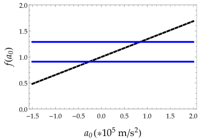
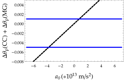
Figure 1: Precession angle against $a_{0}$ assuming $l=5$ Gpc. (i) Left Panel: Dimensionless ratio $f(a_{0})$ for $S_{2}$ data and its bounds. (ii) Right Panel: Precession angle (deviation from GR) $\Delta\theta_{p}(\text{CC})$ + $\Delta\theta_{p}(\text{MG})$ for Mercury data and its bounds.

The bound on $a_{0}$ induces a corresponding bound on $\gamma$, which is computed to be

$$-5.16\times 10^{-14}\ \text{pc}^{-1}\leq\gamma\leq 2.58\times 10^{-13}\ \text{pc}^{-1}.$$ (30)

Previously, an analysis based on galaxy rotation curves showed that, within the dRGT massive gravity, $\gamma\sim 10^{-28}~{}\text{m}^{-1}$ Panpanich:2018cxo . Finally, we also report on the constraint obtained here using the orbital precession of the $S_{2}$ star around Saggitarius $A^{*}$, since, to the best of our knowledge, this is the first attempt to constrain $\gamma$, or equivalently $a_{0}$, upon comparison to the results of GRAVITY Collaboration. We find

$$-2.62\times 10^{-6}~{}\text{m/s}^{2}\leq a_{0}\leq 8.43\times 10^{-6}~{}\text{m/s}^{2}.$$ (31)

although, as already mentioned before, in the discussion to follow we shall use the tighter limits from Mercury.

IV Geodesic Equations and Effective Potential

In this section, we will determine the ISCOs and OSCOs following the steps previously discussed in Boonserm:2019nqq . First, we assume a fixed static, spherically symmetric gravitational background of the form

$$ds^{2}=g_{tt}dt^{2}-g_{rr}dr^{2}-r^{2}[d\theta^{2}+\sin^{2}\theta d\phi^{2}]$$ (32)

Now, following Garcia:2013zud , the equations of motion for test particles are given by

$$\frac{d^{2}x^{\mu}}{ds^{2}}+\Gamma^{\mu}_{\rho\sigma}\frac{dx^{\rho}}{ds}\frac{dx^{\sigma}}{ds}=0$$ (33)

with $s$ as the proper time. The corresponding Christoffel symbols, $\Gamma^{\mu}_{\rho\sigma}$, are computed by landau

$$\Gamma^{\mu}_{\rho\sigma}=\frac{1}{2}g^{\mu\lambda}\left(\frac{\partial g_{\lambda\rho}}{\partial x^{\sigma}}+\frac{\partial g_{\lambda\sigma}}{\partial x^{\rho}}-\frac{\partial g_{\rho\sigma}}{\partial x^{\lambda}}\right).$$ (34)

The mathematical treatment is simplified taking advantage of the fact that there are two conserved quantities (two first integrals of motion), precisely as in the Keplerian problem in classical mechanics. In practice, for $\mu=1=t$ and $\mu=4=\phi$, the geodesic equations acquire the form

$$0 = \frac{d}{ds}\left(g_{tt}\frac{dt}{ds}\right)$$ (35)

$$0 = \frac{d}{ds}\left(r^{2}\frac{d\phi}{ds}\right).$$ (36)

With the above in mind, we then introduce the corresponding conserved quantities as

$$E\equiv g_{tt}\frac{dt}{ds},\;\;\;\;\;\;L\equiv r^{2}\frac{d\phi}{ds}.$$ (37)

The last two quantities, $\{E,L\}$, are usually identified as the energy and angular momentum, respectively.

Assuming a motion on the $(x-y)$ plane (i.e., studying motions on the equatorial plane: $\theta=\pi/2$), the geodesic equation for the $\theta$ index is also satisfied automatically. Therefore, the only non-trivial equation is obtained for $\mu=2=r$ (see Garcia:2013zud for further details)

$$\left(\frac{dr}{ds}\right)^{2}=\frac{1}{g_{tt}g_{rr}}\>\left[E^{2}-g_{tt}\left(\epsilon+\frac{L^{2}}{r^{2}}\right)\right]$$ (38)

which may be also obtained from Garcia:2013zud

$$g_{\mu\nu}\frac{dx^{\mu}}{ds}\frac{dx^{\nu}}{ds}=\epsilon$$ (39)

where $\epsilon=1$ for massive test particles, and $\epsilon=0$ for light rays. In the discussion to follow, we shall consider the case where $\epsilon=1$ (massive test particle with mass $m$) and $g_{tt}g_{rr}=1$. Then, the non-trivial geodesic equation takes the simpler form

$$\left(\frac{dr}{ds}\right)^{2}=\left[E^{2}-g_{tt}\left(1+\frac{L^{2}}{r^{2}}\right)\right]$$ (40)

and we now introduce the corresponding effective potential, which, as usual, is defined to be

$$V(r) =g_{tt}(r)\left(1+\frac{L^{2}}{r^{2}}\right),$$ (41)

where $g_{tt}$ is the lapse function, which will now be identified to $A(r)$ reported in Equation (9) (setting $\eta=0$).

V ISCOs/OSCOs in Massive Gravity

From now on, we will investigate the case of massive particles (which means $\epsilon=1$). The effective potential in this case looks like

$$V(r) =\bigg{(}1-\frac{2M}{r}-\frac{1}{3}\Lambda r^{2}+\gamma r\bigg{)}\bigg{(}1+\frac{L^{2}}{r^{2}}\bigg{)}$$ (42)

and the first and second derivatives of the potential are

$$V^{\prime}(r)=\frac{6L^{2}M}{r^{4}}-\frac{2L^{2}}{r^{3}}+\frac{2M}{r^{2}}-\frac{2r}{l^{2}}+\left(1-\frac{L^{2}}{r^{2}}\right)\gamma$$ (43)

$$V^{\prime\prime}(r)=-\frac{2}{l^{2}}-\frac{24L^{2}M}{r^{5}}+\frac{6L^{2}}{r^{4}}-\frac{4M}{r^{3}}+\frac{2L^{2}}{r^{3}}\gamma$$ (44)

The circular orbits are obtained demanding that

$$\dot{r}=0,\hskip 28.45274pt\text{and}\hskip 28.45274pt\ddot{r}=0,$$ (45)

as function of the rest of parameters. The latter means that we need to find the roots of $V^{\prime}(r)$ for $r\equiv r(L,m,l,\gamma)$. In general, it is not possible to obtain an analytic solution, which is the present case. In order to make progress, we can take an alternative route. From $V^{\prime}(r)=0$, we find $L^{2}$ and evaluate it on $V^{\prime\prime}(r)$ to find the $r_{\text{ISCO}}$ and $r_{\text{OSCO}}$. Thus, we have

$$L^{2} =-\frac{r^{2}\left(2l^{2}M+\gamma l^{2}r^{2}-2r^{3}\right)}{l^{2}\left(6M-\gamma r^{2}-2r\right)}$$ (46)

Similarly to the Kottler spacetime, we reinforce that the angular momentum is real and finite for $r\in(r_{\text{ICCO}},r_{\text{OCCO}}]$. Now, replacing $L^{2}$ into $V^{\prime\prime}(r)$, we have

$$\begin{split}V^{\prime\prime}(r)=&2\frac{-6l^{2}M+l^{2}r-3r^{3}}{l^{2}r^{3}}+\frac{2\gamma}{r}-\\ &\frac{4\left(24l^{2}M^{2}-10l^{2}Mr+l^{2}r^{2}-6Mr^{3}+r^{4}\right)}{l^{2}r^{3}\left(-6M+\gamma r^{2}+2r\right)}\end{split}$$ (47)

To obtain the corresponding roots of $V^{\prime\prime}(r)$, we have to solve the polynomial expression

$$P_{5}(r)=b_{5}r^{5}+b_{4}r^{4}+b_{3}r^{3}+b_{2}r^{2}+b_{1}r+b_{0}$$ (48)

where the parameters are defined as

$$b_{5} =-3\gamma$$ (49)

$$b_{4} =\gamma^{2}l^{2}-8$$ (50)

$$b_{3} =3\gamma l^{2}+30M$$ (51)

$$b_{2} =-12\gamma l^{2}M$$ (52)

$$b_{1} =2l^{2}M$$ (53)

$$b_{0} =-12l^{2}M^{2}$$ (54)

where all lengths are expressed in parsec setting $l=5~{}\text{Gpc}$. There are five roots in total, which, in general, include real (positive or negative) as well as complex roots. We recall that, in the case of the Schwarzschild geometry, there is only one root, $r_{\text{ISCO}}=6M$ Boonserm:2019nqq . Given that there is no analytic expression for the roots of a fifth order polynomial, we shall compute the roots numerically once the numerical values of the parameters are specified.

Thus, we consider three numerical values of the massive gravity parameter $\gamma$ to exemplify how $r_{\text{ISCO}}$ and $r_{\text{OSCO}}$ vary for different structures in the Universe. The first value of $\gamma$ is taken from Panpanich:2018cxo , $\gamma\sim 10^{-28}~{}\text{m}^{-1}$, whereas the remaining two values are obtained in Section III. This is the second main result of the present work summarized in Table 1.

Similarly to the Kottler spacetime, both ISCOs and OSCOs appear. Their numerical values are shown in Table 1, while the astrophysical relevance is shown in Table 2, considering typical values of the mass and size of known structures in the Universe. In particular, our numerical results show that, in all cases, the ISCOs equal $6M$, which is precisely the Schwarzschild result. As far as the OSCOs are concerned, in two of the cases ($\gamma_{1}$ and $\gamma_{2}$), they do not depend on the mass of the astrophysical object. Despite the fact that the OSCOs obtained in those cases are not cosmologically large, their sizes ($2.89\times 10^{7}~{}\text{pc}$ and $2.42\times 10^{6}~{}\text{pc}$, respectively) are similar to the size of cluster of galaxies, which is very large compared to the dimensions of the astrophysical objects displayed in Table 1.

In the third case ($\gamma_{3}$), the OSCOs computed here increase with the mass of the astrophysical object. In addition, their sizes are lower than the ones obtained in the Kottler spacetime Boonserm:2019nqq . In this sense, the OSCOs analysis within the framework of four-dimensional massive gravity reinforces their astrophysical importance. Finally, the fact that the numerical values of the OSCOs obtained here are significantly different than the ones presented in Boonserm:2019nqq indicates that the $\gamma$ term is the dominant one, rather than the cosmological constant term.

VI Conclusions

In summary, we studied the impact of a non-vanishing (positive) cosmological constant on the innermost and outermost stable circular orbits (ISCOs and OSCOs, respectively) within four-dimensional massive gravity. The gravitational field generated by a point-like object is known, and, at the non-relativistic limit, the gravitational potential differs by the Schwarzschild–de Sitter geometry by a term that is linear in the radial coordinate. The numerical value of parameter $\gamma$ of the new, additional term may be determined either using data from the galaxy rotation curves or using data from the periastron advance in the solar system (planet Mercury) and in the Galactic center ($S_{2}$ star).

Starting from the geodesic equations for massive test particles, and the corresponding effective potential, we obtained a polynomial of fifth order that allowed us to compute the innermost and outermost stable circular orbits. We computed its roots numerically for several different structures in the Universe of increasing mass (from the hydrogen atom to stars and globular clusters to galaxies and galaxy clusters) considering three distinct values of the parameter $\gamma$, determined using physical considerations.

Similarly to the Kottler spacetime, both ISCOs and OSCOs appeared. In particular, our numerical results showed that the ISCOs equaled $6M$ (the Schwarzschild result) in all cases; whereas, for OSCOs, in two of the cases ($\gamma_{1}$ and $\gamma_{2}$), this did not depend on the mass of the astrophysical object. In spite of the fact that the OSCOSs obtained in those cases were not cosmologically large, their sizes ($2.89\times 10^{7}$ and $2.42\times 10^{6}$, respectively) were similar to the supercluster size, which is very large compared to the dimensions of the astrophysical objects displayed in Table 1.

In the third case ($\gamma_{3}$), the OSCOs obtained in the present work increased with the mass of the astrophysical object. In addition, their sizes were lower than those obtained in the Kottler spacetime. In this sense, the OSCOs analysis within the framework of four-dimensional massive gravity reinforces their astrophysical importance.

Finally, our numerical results indicate that, within massive gravity, the parameter $\gamma$ played a crucial role in the determination of ISCOs and, more importantly, for OSCOs. Thus, it is $\gamma$, rather than $\Lambda$, as the term that mainly modifies the stable circular orbits, contrary to the Kottler spacetime, where $\Lambda$ is the term producing the new features as far as the OSCOs are concerned.

Acknowlegements

We are grateful to the anonymous reviewers for their constructive criticism as well as numerous useful comments and suggestions. The authors Á.R. and N.C. acknowledge Universidad de Santiago de Chile for financial support through the Proyecto POSTDOC-DICYT, Código 043131 CM-POSTDOC. The authors G.P. and I.L. thank the Fundação para a Ciência e Tecnologia (FCT), Portugal, for the financial support to the Center for Astrophysics and Gravitation-CENTRA, Instituto Superior Técnico, Universidade de Lisboa, through the Project No. UIDB/00099/2020 and grant No. PTDC/FIS-AST/28920/2017.

References

- (1) Freedman, W.L.; Turner, M.S. Measuring and understanding the universe. Rev. Mod. Phys. 2003, 75, 1433.
- (2) Carroll, S.M. The Cosmological constant. Living Rev. Rel. 2001, 4, 1.
- (3) Rubin, V.C.; Ford, W.K., Jr. Rotation of the Andromeda Nebula from a Spectroscopic Survey of Emission Regions. Astrophys. J. 1970, 159, 379.
- (4) Einstein, A. The Foundation of the General Theory of Relativity. Ann. Phys. 1916, 49, 769.
- (5) Sotiriou, T.P.; Faraoni, V. f(R) Theories of Gravity. Rev. Mod. Phys. 2010, 82, 451.
- (6) Felice, A.D.; Tsujikawa, S. f(R) theories. Living Rev. Rel. 2010, 13, 3.
- (7) Brans, C.; Dicke, R.H. Mach’s principle and a relativistic theory of gravitation. Phys. Rev. 1961, 124, 925.
- (8) Brans, C.H. Mach’s Principle and a Relativistic Theory of Gravitation. II. Phys. Rev. 1962, 125, 2194.
- (9) Dicke, R.H. Mach’s principle and invariance under transformation of units. Phys. Rev. 1962, 125, 2163.
- (10) Langlois, D. Brane cosmology: An Introduction. Prog. Theor. Phys. Suppl. 2003, 148, 181.
- (11) Maartens, R. Brane world gravity. Living Rev. Rel. 2004, 7, 7.
- (12) Lovelock, D. The Einstein tensor and its generalizations. J. Math. Phys. 1971, 12, 498-501.
- (13) de Rham, C.; Gabadadze, G. Generalization of the Fierz-Pauli Action. Phys. Rev. D 2010, 82, 044020.
- (14) de Rham, C.; Gabadadze, G.; Tolley, A.J. Resummation of Massive Gravity. Phys. Rev. Lett. 2011, 106, 231101.
- (15) Ghosh, S.G.; Tannukij, L.; Wongjun, P. A class of black holes in dRGT massive gravity and their thermodynamical properties. Eur. Phys. J. C 2016, 76, 119.
- (16) Schwarzschild, K. On the Gravitational Field of a Mass Point According to Einstein’s Theory; Sitzungsberichte der Preussischen Akademie der Wissenschaften: Berlin, Germany, 1916; p. 189.
- (17) Panpanich, S.; Burikham, P. Fitting rotation curves of galaxies by de Rham-Gabadadze-Tolley massive gravity. Phys. Rev. D 2018, 98, 064008.
- (18) Ashtekar, A. Implications of a positive cosmological constant for general relativity. Rept. Prog. Phys. 2017, 80, 102901.
- (19) Boonserm, P.; Ngampitipan, T.; Simpson, A.; Visser, M. Innermost and outermost stable circular orbits in the presence of a positive cosmological constant. Phys. Rev. D 2020, 101, 024050.
- (20) Rezzolla, L.; Zanotti, O.; Font, J.A. Dynamics of thick discs around Schwarzschild–de Sitter black holes. Astron. Astrophys. 2003, 412, 603.
- (21) Stuchlik, Z. Influence of the relict cosmological constant on accretion discs. Mod. Phys. Lett. A 2005, 20, 561.
- (22) Stuchlik, Z.; Schee, J. Influence of the cosmological constant on the motion of Magellanic Clouds in the gravitational field of Milky Way. JCAP 2011, 09, 018.
- (23) Sarkar, T.; Ghosh, S.; Bhadra, A. Newtonian analogue of Schwarzschild de-Sitter spacetime: Influence on the local kinematics in galaxies. Phys. Rev. D 2014, 90, 063008.
- (24) Perez, D.; Romero, G.E.; Bergliaffa, S.E.P. Accretion disks around black holes in modified strong gravity. Astron. Astrophys. 2013, 551, A4.
- (25) Lee, H.C.; Han, Y.J. Innermost stable circular orbit of Kerr-MOG black hole. Eur. Phys. J. C 2017, 77, 655.
- (26) Koch, B.; Reyes, I.A.; Rincon, A. A scale dependent black hole in three-dimensional space–time. Class. Quant. Grav. 2016, 33, 225010.
- (27) Rincon, A.; Koch, B.; Reyes, I. BTZ black hole assuming running couplings. J. Phys. Conf. Ser. 2017, 831, 012007.
- (28) Rincon, A.; Contreras, E.; Bargueño, P.; Koch, B.; Panotopoulos, G.; Hernandez-Arboleda, A. Scale dependent three-dimensional charged black holes in linear and non-linear electrodynamics. Eur. Phys. J. C 2017, 77, 494.
- (29) Rincon, A.; Panotopoulos, G. Quasinormal modes of scale dependent black holes in (1+2)-dimensional Einstein-power-Maxwell theory. Phys. Rev. D 2018, 97, 024027.
- (30) Contreras, E.; Rincon, A.; Koch, B.; Bargueño, P. Scale-dependent polytropic black hole. Eur. Phys. J. C 2018, 78, 246.
- (31) Rincon, A.; Koch, B. Scale-dependent rotating BTZ black hole. Eur. Phys. J. C 2018, 78, 1022.
- (32) Rincon, A.; Contreras, E.; Bargueño, P.; Koch, B.; Panotopoulos, G. Scale-dependent ()-dimensional electrically charged black holes in Einstein-power-Maxwell theory. Eur. Phys. J. C 2018, 78, 641.
- (33) Rincon, A.; Contreras, E.; Bargueño, P.; Koch, B. Scale-dependent planar Anti-de Sitter black hole. Eur. Phys. J. Plus 2019, 134, 557.
- (34) Contreras, E.; Rincon, A.; Panotopoulos, G.; Bargueño, P.; Koch, B. Black hole shadow of a rotating scale–dependent black hole. Phys. Rev. D 2020, 101, 064053.
- (35) Rincon, A.; Panotopoulos, G. Scale-dependent slowly rotating black holes with flat horizon structure. Phys. Dark Univ. 2020, 30, 100725.
- (36) Panotopoulos, G.; Rincon, A. Quasinormal spectra of scale-dependent Schwarzschild–de Sitter black holes. Phys. Dark Univ. 2021, 31, 100743, doi:10.1016/j.dark.2020.100743.
- (37) Rincon, A.; Villanueva, J.R. The Sagnac effect on a scale-dependent rotating BTZ black hole background. Class. Quant. Grav. 2020, 37, 175003.
- (38) Fathi, M.; Rincon, A.; Villanueva, J.R. Photon trajectories on a first order scale-dependent static BTZ black hole. Class. Quant. Grav. 2020, 37, 075004.
- (39) Contreras, E.; Rincon, A.; Bargueno, P. Five-dimensional scale-dependent black holes with constant curvature and Solv horizons. Eur. Phys. J. C 2020, 80, 367.
- (40) Panotopoulos, G.; Rincon, A.; Lopes, I. Interior solutions of relativistic stars in the scale-dependent scenario. Eur. Phys. J. C 2020, 80, 318.
- (41) Panotopoulos, G.; Rincon, A.; Lopes, I. Interior solutions of relativistic stars with anisotropic matter in scale-dependent gravity. Eur. Phys. J. C 2021, 81, 63.
- (42) Canales, F.; Koch, B.; Laporte, C.; Rincon, A. Cosmological constant problem: Deflation during inflation. JCAP 2020, 2001, 021.
- (43) Alvarez, P.D.; Koch, B.; Laporte, C.; Rincón, Á. Can scale-dependent cosmology alleviate the tension? JCAP 2021, 6, 019.
- (44) Cai, R.G. Gauss-Bonnet black holes in AdS spaces. Phys. Rev. D 2002, 65, 084014.
- (45) Berezhiani, L.; Chkareuli, G.; de Rham, C.; Gabadadze, G.; Tolley, A.J. On Black Holes in Massive Gravity. Phys. Rev. D 2012, 85, 044024.
- (46) Burikham, P.; Harko, T.; Lake, M.J. Mass bounds for compact spherically symmetric objects in generalized gravity theories. Phys. Rev. D 2016, 94, 064070.
- (47) Kareeso, P.; Burikham, P.; Harko, T. Mass-radius ratio bounds for compact objects in Massive Gravity theory. Eur. Phys. J. C 2018, 78, 941.
- (48) Boonserm, P.; Ngampitipan, T.; Wongjun, P. Greybody factor for black string in dRGT massive gravity. Eur. Phys. J. C 2019, 79, 330.
- (49) Landau, L.D.; Lifschits, E.M. The Classical Theory of Fields, 3rd ed.; Course of Theoretical Physics Volume 2; Pergamon Press: Oxford, UK.
- (50) Wald, R.M. General Relativity; University of Chicago Press: Chicago, IL, USA, 1984.
- (51) Jafari, G.; Setare, M.R.; Bakhtiarizadeh, H.R. Static spherically symmetric black holes of de Rham–Gabadadze–Tolley massive gravity in arbitrary dimensions. Phys. Lett. B 2017, 773, 395-400.
- (52) Li, P.; Li, X.z.; Xi, P. Black hole solutions in de Rham-Gabadadze-Tolley massive gravity. Phys. Rev. D 2016, 93, 064040.
- (53) Koyama, K.; Niz, G.; Tasinato, G. Analytic solutions in non-linear massive gravity. Phys. Rev. Lett. 2011, 107, 131101.
- (54) Koyama, K.; Niz, G.; Tasinato, G. Strong interactions and exact solutions in non-linear massive gravity. Phys. Rev. D 2011, 84, 064033.
- (55) Adkins, G.S.; McDonnell, J. Orbital precession due to central-force perturbations. Phys. Rev. D 2007, 75, 082001.
- (56) Zakharov, A. Constraints on alternative theories of gravity with observations of the Galactic Center. EPJ Web Conf. 2018, 191, 01010.
- (57) Clifton, T.; Carrilho, P.; Fernandes, P.G.S.; Mulryne, D.J. Observational Constraints on the Regularized 4D Einstein-Gauss-Bonnet Theory of Gravity. Phys. Rev. D 2020, 102, 084005.
- (58) Pitjeva, E.V.; Pitjev, N.P. Relativistic effects and dark matter in the Solar system from observations of planets and spacecraft. Mon. Not. Roy. Astron. Soc. 2013, 432, 3431.
- (59) Abuter, R.; Amorim, A.; Bauböck, M.; Berger, J.P.; Bonnet, H.; Brandner, W.; Cardoso, V.; Clénet, Y.; de Zeeuw, P.T.; Dexter, J.; et al. Detection of the Schwarzschild precession in the orbit of the star S2 near the Galactic centre massive black hole. Astron. Astrophys. 2020, 636, L5.
- (60) García, A.; Hackmann, E.; Kunz, J.; Lämmerzahl, C.; Macías, A. Motion of test particles in a regular black hole space–time. J. Math. Phys. 2015, 56, 032501.