Visual Boundary Knowledge Translation for Foreground Segmentation

Abstract

When confronted with objects of unknown types in an image, humans can effortlessly and precisely tell their visual boundaries. This recognition mechanism and underlying generalization capability seem to contrast to state-of-the-art image segmentation networks that rely on large-scale category-aware annotated training samples. In this paper, we make an attempt towards building models that explicitly account for visual boundary knowledge, in hope to reduce the training effort on segmenting unseen categories. Specifically, we investigate a new task termed as Boundary Knowledge Translation (BKT). Given a set of fully labeled categories, BKT aims to translate the visual boundary knowledge learned from the labeled categories, to a set of novel categories, each of which is provided only a few labeled samples. To this end, we propose a Translation Segmentation Network (Trans-Net), which comprises a segmentation network and two boundary discriminators. The segmentation network, combined with a boundary-aware self-supervised mechanism, is devised to conduct foreground segmentation, while the two discriminators work together in an adversarial manner to ensure an accurate segmentation of the novel categories under light supervision. Exhaustive experiments demonstrate that, with only tens of labeled samples as guidance, Trans-Net achieves close results on par with fully supervised methods.

Introduction

Image segmentation has witnessed an unprecedented development in the past decade thanks to the deep learning. The encouraging results, however, come at the cost of the vast number of annotations and GPU training for days or even weeks. To alleviate the training effort, a number of learning techniques, such as few-shot learning and transfer learning, have proposed. The former aims to train models using only a few annotated samples, while the later focuses on transferring the models learned on one domain to another novel one. Despite the recent progress in few-shot and transfer learning, existing approaches are still prone to either inferior results (Shaban et al. 2017; Siam, Oreshkin, and Jagersand 2019; Wang et al. 2019a), or the rigorous requirement that the two tasks are strongly related (Dai et al. 2019; Sun et al. 2019) and a large number of annotated samples (Hong et al. 2017; Li, Arnab, and Torr 2018; Papandreou et al. 2015).

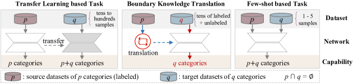
Figure 1: Comparing the proposed BKT with transfer learning and few-shot learning. Specifically, BKT translates the knowledge learned from $p$ training categories into another $q$ ones, where the $p$ and $q$ categories are disjoint. Unlike transfer learning and few-shot learning based tasks where the trained models eventually tackle $p+q$ categories, BKT concentrates on the $q$ testing categories only.

Nevertheless, our human eyes can effortlessly recognize the visual boundary of a scene object, even if this object seems unfamiliar or belongs to an unknown category. Inspired by this fact, we study in this paper a new Boundary Knowledge Translation Task (BKT-Task), in aim to translate the knowledge learned from $p$ training categories where abundant annotations are available, into another $q$ target categories where a very small number of annotations are available for each class.

The differences between the proposed BKT-Task and the two related tasks, transfer learning and few-shot learning, are summarized in Fig. 1. Unlike transfer learning that requires the $p$ source categories and the $q$ target ones to be highly related so as to achieve reasonable performances, in BKT such requirement is largely relaxed. As demonstrated in our experiments, for example, the visual boundary knowledge of birds can be seamlessly translated into the segmentation network for flowers. Also, in contrast to both transfer and few-shot learning, whose outputs span $p+q$ categories, BKT focuses on the $q$ categories only, which seems to be a flaw of BKT but in reality not. In many cases, since abundant annotations are available for the $p$ categories, indicating that state-of-the-art deep networks will highly likely to deliver gratifying results, a model that focuses on the novel $q$ categories where annotations are insufficient is much desired. Furthermore, as shown in prior works (Chen, Artieres, and Denoyer 2019; Minaee et al. 2020; Vinyals et al. 2016) and also demonstrated in our experiments, handling many categories simultaneously at once, especially under a compact network architecture, will significantly downgrade the performances for all classes; focusing on the $q$ critical categories, on the other hand, will alleviate this dilemma to a large extend and ensure satisfactory performances.

To this end, we propose a Translation Segmentation Network (Trans-Net) for the above BKT-Task. The Trans-Net is designed to contain a segmentation network and two boundary discriminators. The segmentation network focuses on only segmenting the target categories, while the two discriminators collaborate in an adversarial fashion: one works on distinguishing whether the segmented foreground contains the background features, and the other distinguishes whether the segmented background contains the foreground features. Meanwhile, we also introduce pseudo masks for enhancing and accelerating the translation of the boundary knowledge.

For the segmentation network, we label tens of samples of the target categories, as the guidance for segmenting the desired boundary of the foreground. We also propose a self-supervised strategy to strengthen the boundary consistency of unlabeled samples. Through the adversarial optimization, the visual boundary knowledge of fully labeled $p$ categories can be effectively translated into the segmentation network by two boundary discriminators. Experiments demonstrate that, with only tens of labeled samples as guidance, Trans-Net achieves truly encouraging results on par with fully supervised methods.

Our contribution is therefore introducing the new BKT-Task, in aim to translate the visual boundary knowledge learned from fully annotate source categories into novel ones with few labels, and proposing a dedicated solution, Trans-Net, towards solving BKT-Task. As the first attempt along its line, Trans-Net, for the time being, focuses on foreground segmentation. We devise a boundary-aware self-supervised mechanism and pseudo masks for the segmentation network and the discriminators to enhance the translation of visual boundary knowledge, respectively. We evaluate the proposed Trans-Net on a broad domain of image datasets, in term of both qualitative visualization and quantitative measures, and show that the proposed method achieves results on par with fully supervised ones.

Related work

We briefly review here two lines of work that are related to ours, GAN-based segmentation methods and boundary-aware segmentation. More related works about few-shot learning and transfer learning are given in the supplementary materials.

GAN-based segmentation methods can be classified into two categories: mask distribution-based methods and composition fidelity based methods. For the mask distribution-based methods, Luc et al. (2016) proposed the first GAN based semantic segmentation network, which adopts the adversarial optimization between segmented results and GT mask to train the segmentation network. Meanwhile, some researchers (Arbelle and Raviv 2018; Han and Yin 2017; Xue et al. 2018) applied the same adversarial strategy into medical image segmentation. With generated fake images and labeled images, Souly, Spampinato, and Shah (2017) adopted the adversarial strategy to train the discriminator output class confidence maps. Furthermore, Hung et al. (2018) extended the discriminator to generate a confidence map, which can be used to infer the regions sufficiently close to those from the ground truth distribution. In the composition fidelity based methods (Chen, Artieres, and Denoyer 2019; Ostyakov et al. 2018; Remez, Huang, and Brown 2018), the segmented objects are firstly composited with some background images. Then, the discriminator is adopted to discriminate fidelity of the composited images and the GT nature images. Unlike the above existing GAN-based methods, we adopt the adversarial strategy to translate the source categories’ visual boundary knowledge into the segmentation network by two boundary discriminators.

Boundary-aware segmentation. Bertasius, Shi, and Torresani (2016) proposed two-tream framework where the predicted semantic boundaries is adopted to improve the semantic segmentation maps. Similarly, two-tream framework is also adopted in some recent works (Chen et al. 2016; Cheng et al. 2017; Yu et al. 2018; Takikawa et al. 2019a), where different constraints are devised for strengthening the segmentation results with the predicted boundaries. Unlike predicting the boundary directly,  Hayder, He, and Salzmann (2017) proposed predicting pixels’ distance to the object’s boundary and post-processed the distance map into the final segmented results. Zhang et al. (2017) proposed a local boundary refinement network to learn the position-adaptive propagation coefficients so that local contextual information from neighbors can be optimally captured for refining object boundaries. Peng et al. (2017) proposed a boundary refinement block to improve the localization performance near the object boundaries. Khoreva et al. (2017) proposed boundary-aware filtering to improve object delineation. Qin et al. (2019) adopted the patch-level SSIM loss (Wang, Simoncelli, and Bovik 2003) to assign higher weights to the boundary. Unlike the above methods, we devise two boundary discriminators for discriminating the foreground’s outer border and background’s inner boundary, which can translate the visual boundary knowledge into a segmentation network for any new category.

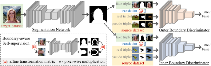
Figure 2: The framework of Trans-Net. The segmentation network is designed to segment the sample’s foreground in the target dataset. The outer boundary discriminator is devised for distinguishing whether the segmented foreground contains the outer background’s features. The inner boundary discriminator is devised for distinguishing whether the segmented background contains the inner foreground’s features. Pseudo samples of source dataset are generated with the eroded and dilated masks, which can reinforce the visual boundary knowledge translation. Boundary-aware self-supervision is proposed to constrain the boundary invariance on the target dataset.

Boundary Knowledge Translation Task

The definition of the BKT-Task is given as follows. We assume that we are given the labeled source dataset $\mathbf{S}^{p}$ that contains $p$ object categories and target dataset $\mathbb{S}^{q}$ of $q$ object categories. The $p$ categories and $q$ categories are disjoint. The visual boundary knowledge is defined as the perfect segmentation that the object doesn’t contain outer background’s features, and the background doesn’t contain inner objects’ features. The goal of BKT-Task is to translate the visual boundary knowledge of $\mathbf{S}^{p}$ into the segmentation network $\mathcal{F}_{\theta}$, which is devised for only concentrating on the segmentation of $q$ categories. The difference between the BKT-Task and other related tasks are shown in Fig. 1.

Method

There are vast public labeled datasets for the segmentation task. The BKT-Task can effectively exploit those source datasets into the segmentation network for a new category, which will dramatically reduce the requirement for labeled samples in the new category. As the first attempt along BKT-Task, in this paper, we focus on foreground segmentation and propose a Translation Segmentation Network (Trans-Net), shown in Fig. 2. Trans-Net contains a segmentation network and two boundary discriminators. The segmentation network is designed for only segment samples in the target dataset $\mathbb{S}^{q}$. The two boundary discriminators are devised for translating visual boundary knowledge of the source dataset $\mathbf{S}^{p}$ into the segmentation network without embezzling its capability for $q$ categories.

Segmentation Network

In Trans-Net, the segmentation network $\mathcal{F}_{\theta}$ is designed to be an encoder-decoder architecture. Given a target image $\overline{\textbf{\em x}}\in\mathbb{S}^{q}$, the segmented result $\tilde{\textbf{\em m}}=\mathcal{F}_{\theta}(\overline{\textbf{\em x}})$ is expected to approximate the GT mask m, which can be achieved by minimizing the following basic reconstruction loss $\mathbf{\mathcal{L}_{rec}}$:

$$\mathbf{\mathcal{L}_{rec}}=||\tilde{\textbf{\em m}}-\textbf{\em m}||^{2}_{2},~{}\tilde{\textbf{\em m}}=\mathcal{F}_{\theta}(\overline{\textbf{\em x}}),~{}\overline{\textbf{\em x}}\in\mathbb{S}^{q}.$$ (1)

The $\mathbf{\mathcal{L}_{rec}}$ is used to reconstruct a few labeled samples of the target datasets, which will guide the segmentation of the desired boundary.

Boundary-aware Self-supervision. To reduce the amount of labelled samples, inspired by Wang et al. (2019b), we propose a boundary-aware self-supervised strategy, which can strengthen the boundary consistency on target categories. The core idea is that the segmented result of the warped input image should be equal to the warped result of the input image. The schematic diagram of boundary-aware self-supervision is given in Fig. 2. Formally, for the robust segmentation network, given an affine transformation matrix A, segmented result $\mathcal{F}_{\theta}(\textbf{\em A}\overline{\textbf{\em x}})$ of the warped image $\textbf{\em A}\overline{\textbf{\em x}}$ and the warped result $\textbf{\em A}\mathcal{F}_{\theta}(\overline{\textbf{\em x}})$ should be consistent in the following way: $\mathcal{F}_{\theta}(\textbf{\em A}\overline{\textbf{\em x}})=\textbf{\em A}\mathcal{F}_{\theta}(\overline{\textbf{\em x}})$. Furthermore, we obtain the boundary neighborhood weight map w as follows:

$$\textbf{\em w}=\mathfrak{D}_{r}(\tilde{\textbf{\em m}})-\mathfrak{E}_{r}(\tilde{\textbf{\em m}}),$$ (2)

where, $\mathfrak{D}_{r}$ and $\mathfrak{E}_{r}$ denote the dilation and erosion operation with disk strel of radius $r$. The weight map w can further strengthen the boundary consistency. The boundary-aware self-supervised loss $\mathbf{\mathcal{L}_{sel}}$ is defined as follows:

$$\mathbf{\mathcal{L}_{sel}}=||\textbf{\em w}^{\prime}\mathcal{F}_{\theta}(\textbf{\em A}\overline{\textbf{\em x}})-\textbf{\em A}\{\textbf{\em w}\mathcal{F}_{\theta}(\overline{\textbf{\em x}})\}||^{2}_{2},~{}\overline{\textbf{\em x}}\in\mathbb{S}^{q},$$ (3)

where, $\textbf{\em w}^{\prime}$ and w are the weight maps of the predict masks $\mathcal{F}_{\theta}(\textbf{\em A}\overline{\textbf{\em x}})$ and $\mathcal{F}_{\theta}(\overline{\textbf{\em x}})$, respectively. The boundary-aware self-supervised mechanism not only strengthens the boundary consistency but also can eliminate the unreasonable holes in the predict masks.

Boundary Discriminator

Inspired by the fact that humans can segment an object’s boundary through distinguishing whether the inner and outer of boundary contain redundant features, we devise two boundary discriminators, which can translate the boundary knowledge of the source dataset $\mathbf{S}^{p}$ into the segmentation network.

Outer Boundary Discriminator. Given the input target image $\overline{\textbf{\em x}}\in\mathbb{S}^{q}$, the segmentation network predicts the mask $\tilde{\textbf{\em m}}=\mathcal{F}_{\theta}(\overline{\textbf{\em x}})$. Next, the foreground $\overline{\textbf{\em x}}^{o}$ is computed using the following equation: $\overline{\textbf{\em x}}^{o}=\tilde{\textbf{\em m}}*\overline{\textbf{\em x}}$, where ‘$*$’ denotes pixel-wise multiplication. Then the concatenated triplet $\textbf{\em I}^{o}_{a}=[\overline{\textbf{\em x}},\tilde{\textbf{\em m}},\overline{\textbf{\em x}}^{o}]$ is input into the outer boundary discriminator $\mathcal{D}^{o}_{\phi}$, which discriminates whether the segmented foreground $\overline{\textbf{\em x}}^{o}$ contains the background’s outer features. In the paper, $\textbf{\em I}^{o}_{a}$ is regarded as a fake triplet. Meanwhile, choosing a labeled sample $\underline{\textbf{\em x}}$ from the source dataset $\mathbf{S}^{p}$, the corresponding $\textbf{\em I}^{o}_{e}=[\underline{\textbf{\em x}},\textbf{\em m},\underline{\textbf{\em x}}^{o}]$ is labeled as a real triplet. Furthermore, we reprocess the GT mask m of samples $\underline{\textbf{\em x}}\in\mathbf{S}^{p}$ by dilation operation and get the pseudo triplet $\textbf{\em I}^{o}_{s}=[\underline{\textbf{\em x}},\mathfrak{D}_{r}(\textbf{\em m}),\underline{\textbf{\em x}}^{o}_{\mathfrak{D}}]$, where $\underline{\textbf{\em x}}\in\mathbf{S}^{p}$ and $\underline{\textbf{\em x}}^{o}_{\mathfrak{D}}=\mathfrak{D}_{r}(\textbf{\em m})*\underline{\textbf{\em x}}$. The generated pseudo triplet $\textbf{\em I}^{o}_{s}$ will assist the outer boundary discriminator in distinguishing the background’s outer features. The adversarial optimization between the segmentation network and outer boundary discriminator will translate the outer boundary knowledge of the source dataset $\mathbf{S}^{p}$ into the segmentation network with the following outer boundary adversarial loss $\mathbf{\mathcal{L}^{out}_{adv}}$:

$$\begin{split}\mathbf{\mathcal{L}^{out}_{adv}}\!\!=&\frac{1}{2}\!\mathop{\mathbb{E}}\limits_{\textbf{\em I}^{o}_{a}\sim\mathbb{P}^{o}_{a}}\![\mathcal{D}^{o}_{\phi}\!(\textbf{\em I}^{o}_{a})]\!+\!\frac{1}{2}\!\mathop{\mathbb{E}}\limits_{\textbf{\em I}^{o}_{s}\sim\mathbb{P}^{o}_{s}}[\mathcal{D}^{o}_{\phi}\!(\textbf{\em I}^{o}_{s})]\!-\!\!\!\!\mathop{\mathbb{E}}\limits_{\textbf{\em I}^{o}_{e}\sim\mathbb{P}^{o}_{e}}\![\mathcal{D}^{o}_{\phi}\!(\textbf{\em I}^{o}_{e})]\\ &+\lambda\!\mathop{\mathbb{E}}\limits_{\textbf{\em I}^{o}\sim\mathbb{P}_{\textbf{\em I}^{o}}}\!\![(\|\nabla_{\textbf{\em I}^{o}}\mathcal{D}^{o}_{\phi}(\textbf{\em I}^{o})\|_{2}\!-\!1)^{2}],\end{split}$$ (4)

where, the $\mathbb{P}^{o}_{a}$, $\mathbb{P}^{o}_{s}$, $\mathbb{P}^{o}_{e}$ are the segmented outer boundary distribution, pseudo outer boundary distribution, and real outer boundary distribution, respectively. The $\mathbb{P}_{\textbf{\em I}^{o}}$ is sampled uniformly along straight lines between pairs of points sampled from the distribution $\mathbb{P}^{o}_{e}$ and the segmentation network distribution $\mathbb{P}^{o}_{a}$. The $\textbf{\em I}^{o}=\varepsilon\textbf{\em I}^{o}_{e}+(1-\varepsilon)\textbf{\em I}^{o}_{a}$, where the $\varepsilon$ is a random number between $0$ and $1$. The gradient penalty term is firstly proposed in WGAN-GP (Gulrajani et al. 2017). The $\lambda$ is the gradient penalty coefficient.

Algorithm 1 The Training Algorithm for Trans-Net

1: The gradient penalty coefficient $\lambda$, interval iteration number $n_{critic}$, the batch size $K$, Adam hyperparameters $\alpha,\beta_{1},\beta_{2}$, the balance parameters $\tau,\eta$ for $\mathcal{L}_{rec}$ and $\mathbf{\mathcal{L}_{sel}}$, the Laplace smoothing parameter $\xi$.

2: Initial critic parameters $\varphi,\phi$, initial segmentation network parameters $\theta$.

3:while $\theta$ has not converged do

4:     for $t=1,...,n_{critic}$ do

5:         for $k=1,...,K$ do

6:              Sample $\overline{\textbf{\em x}}$ from target dataset $\mathbb{S}^{q}$, $(\underline{\textbf{\em x}},\textbf{\em m})$ from source dataset $\mathbf{S}^{p}$, a random number $\varepsilon\sim U[0,1]$.

7:              Obtain real triplet $\textbf{\em I}^{o}_{e}=[\underline{\textbf{\em x}},\textbf{\em m},\underline{\textbf{\em x}}^{o}]$ and $\textbf{\em I}^{i}_{e}=[\underline{\textbf{\em x}},\textbf{\em m}^{\prime},\underline{\textbf{\em x}}^{i}]$, $\underline{\textbf{\em x}}^{o}=\textbf{\em m}*\underline{\textbf{\em x}}$, $\underline{\textbf{\em x}}^{i}=\textbf{\em m}^{\prime}*\underline{\textbf{\em x}}$.

8:              Obtain fake triplet $\textbf{\em I}^{o}_{a}=[\overline{\textbf{\em x}},\tilde{\textbf{\em m}},\overline{\textbf{\em x}}^{o}]$ and $\textbf{\em I}^{i}_{a}=[\overline{\textbf{\em x}},\tilde{\textbf{\em m}}^{\prime},\overline{\textbf{\em x}}^{i}]$, $\tilde{\textbf{\em m}}=\mathcal{F}_{\theta}(\overline{\textbf{\em x}})$, $\tilde{\textbf{\em m}}^{\prime}=[\mathbf{1}]-\tilde{\textbf{\em m}}$.

9:              Obtain pseudo triplet $\textbf{\em I}^{o}_{s}=[\underline{\textbf{\em x}},\mathfrak{D}_{r}(\textbf{\em m}),\underline{\textbf{\em x}}^{o}_{\mathfrak{D}}]$ and $\textbf{\em I}^{i}_{s}=[\underline{\textbf{\em x}},\mathfrak{E}_{r}(\textbf{\em m}^{\prime}),\underline{\textbf{\em x}}^{i}_{\mathfrak{E}}]$.

10:              $\textbf{\em I}^{o}\leftarrow\varepsilon\textbf{\em I}^{o}_{e}+(1-\varepsilon)\textbf{\em I}^{o}_{a}$, $\textbf{\em I}^{i}\leftarrow\varepsilon\textbf{\em I}^{i}_{e}+(1-\varepsilon)\textbf{\em I}^{i}_{a}$.

11:              $\mathbf{\mathcal{L}^{out}_{adv}}^{(k)}\leftarrow\frac{1}{2}\mathcal{D}^{o}_{\phi}(\textbf{\em I}^{o}_{a})+\frac{1}{2}\mathcal{D}^{o}_{\phi}(\textbf{\em I}^{o}_{s})-\mathcal{D}^{o}_{\phi}(\textbf{\em I}^{o}_{e})+$

12:         $\lambda(\|\nabla_{\textbf{\em I}^{o}}\mathcal{D}^{o}_{\phi}(\textbf{\em I}^{o})\|_{2}-1)^{2}$.

13:              $\mathbf{\mathcal{L}^{in}_{adv}}^{(k)}\leftarrow\frac{1}{2}\mathcal{D}^{i}_{\varphi}(\textbf{\em I}^{i}_{a})+\frac{1}{2}\mathcal{D}^{i}_{\varphi}(\textbf{\em I}^{i}_{s})-\mathcal{D}^{i}_{\varphi}(\textbf{\em I}^{i}_{e})+$

14:         $\lambda(\|\nabla_{\textbf{\em I}^{i}}\mathcal{D}^{i}_{\varphi}(\textbf{\em I}^{i})\|_{2}-1)^{2}$.          

15:         $\phi\leftarrow Adam(\nabla_{\phi}\frac{1}{K}\sum^{K}_{k=1}\mathbf{\mathcal{L}^{out}_{adv}}^{(k)},\phi,\alpha,\beta_{1},\beta_{2})$.

16:         $\varphi\leftarrow Adam(\nabla_{\varphi}\frac{1}{K}\sum^{K}_{k=1}\mathbf{\mathcal{L}^{in}_{adv}}^{(k)},\varphi,\alpha,\beta_{1},\beta_{2})$.      

17:     Sample unlabeled batch $\{\overline{\textbf{\em x}}^{(k)}\}^{K}_{k=1}$ and labeled batch $\{\ddot{\overline{\textbf{\em x}}}^{(k)},\textbf{\em m}^{(k)}\}^{K}_{k=1}$ from target dataset $\mathbb{S}^{q}$.

18:     $\mathbf{\mathcal{L}_{rec}}\leftarrow||\mathcal{F}_{\theta}(\ddot{\overline{\textbf{\em x}}})-\textbf{\em m}||^{2}_{2}$.

19:     $\mathbf{\mathcal{L}_{sel}}\leftarrow||\textbf{\em w}^{\prime}\mathcal{F}_{\theta}(\textbf{\em A}\overline{\textbf{\em x}})-\textbf{\em A}\{\textbf{\em w}\mathcal{F}_{\theta}(\overline{\textbf{\em x}})\}||^{2}_{2}$.

20:     $\theta\leftarrow Adam(\nabla_{\theta}\frac{1}{K}\sum^{K}_{k=1}\{\mathbf{\tau\mathcal{L}_{rec}}+\eta\mathbf{\mathcal{L}_{sel}}-\mathcal{D}^{o}_{\phi}(\mathcal{F}_{\theta}(\overline{\textbf{\em x}}))-\mathcal{D}^{i}_{\varphi}(\mathcal{F}_{\theta}(\overline{\textbf{\em x}}))\}),\theta,\alpha,\beta_{1},\beta_{2})$.

21:return Segmentation network parameters $\theta$, critic parameters $\varphi,~{}\phi$.

Inner Boundary Discriminator. The inner boundary discriminator $\mathcal{D}^{i}_{\varphi}$ is devised for discriminating whether the segmented background contains the object’s inner features. To obtain the segmented background, the predict background mask $\tilde{\textbf{\em m}}^{\prime}$ and GT mask $\textbf{\em m}^{\prime}$ are reprocessed with the Not-operation as follows: $\tilde{\textbf{\em m}}^{\prime}=[\mathbf{1}]-\tilde{\textbf{\em m}}$, $\textbf{\em m}^{\prime}=[\mathbf{1}]-\textbf{\em m}$, where the $[\mathbf{1}]$ denotes the unit matrix of m’s size. Then, the corresponding fake triplet $\textbf{\em I}^{i}_{a}=[\overline{\textbf{\em x}},\tilde{\textbf{\em m}}^{\prime},\overline{\textbf{\em x}}^{i}]$, real triplet $\textbf{\em I}^{i}_{e}=[\underline{\textbf{\em x}},\textbf{\em m}^{\prime},\underline{\textbf{\em x}}^{i}]$ and pseudo triplet $\textbf{\em I}^{i}_{s}=[\underline{\textbf{\em x}},\mathfrak{D}_{r}(\textbf{\em m}^{\prime}),\underline{\textbf{\em x}}^{i}_{\mathfrak{D}}]$ are computed in the same manner as done in the outer boundary discriminator. The generated pseudo triplet $\textbf{\em I}^{i}_{s}$ will also assist the inner boundary discriminator in distinguishing the inner features of the foreground. Similarly, the inner boundary adversarial loss $\mathbf{\mathcal{L}^{in}_{adv}}$ is defined as follows:

$$\begin{split}\mathbf{\mathcal{L}^{in}_{adv}}\!\!=&\frac{1}{2}\!\mathop{\mathbb{E}}\limits_{\textbf{\em I}^{i}_{a}\sim\mathbb{P}^{i}_{a}}\![\mathcal{D}^{i}_{\varphi}\!(\textbf{\em I}^{i}_{a})]\!+\!\frac{1}{2}\!\mathop{\mathbb{E}}\limits_{\textbf{\em I}^{i}_{s}\sim\mathbb{P}^{i}_{s}}[\mathcal{D}^{i}_{\varphi}\!(\textbf{\em I}^{i}_{s})]\!-\!\!\!\!\mathop{\mathbb{E}}\limits_{\textbf{\em I}^{i}_{e}\sim\mathbb{P}^{i}_{e}}\![\mathcal{D}^{i}_{\varphi}\!(\textbf{\em I}^{i}_{e})]\\ &+\lambda\!\mathop{\mathbb{E}}\limits_{\textbf{\em I}^{i}\sim\mathbb{P}_{\textbf{\em I}^{i}}}\!\![(\|\nabla_{\textbf{\em I}^{i}}\mathcal{D}^{i}_{\varphi}(\textbf{\em I}^{i})\|_{2}\!-\!1)^{2}],\end{split}$$ (5)

where, the $\mathbb{P}^{i}_{a}$, $\mathbb{P}^{i}_{s}$, $\mathbb{P}^{i}_{e}$ are the segmented inner boundary distribution, pseudo inner boundary distribution, and real inner boundary distribution, respectively. $\textbf{\em I}^{i}=\varepsilon\textbf{\em I}^{i}_{e}+(1-\varepsilon)\textbf{\em I}^{i}_{a}$. The optimization on $\mathbf{\mathcal{L}^{in}_{adv}}$ will translate the inner boundary knowledge of the source dataset $\mathbf{S}^{p}$ into the segmentation network.

\begin{overpic}[scale={0.60}]{Figures/visualResults.pdf} { \put(2.0,46.8){Input} \put(9.1,46.8){GT} \put(16.0,46.8){CAC} \put(23.1,46.8){ReDO} \put(29.0,46.8){SG-One} \put(36.8,46.8){PANet} \put(44.0,46.8){SPNet} \put(51.0,46.8){CANet} \put(58.0,46.8){ALSSS} \put(65.5,46.8){USSS} \put(70.5,46.8){Trans.(10)} \put(78.2,46.8){Trans.(100)} \put(87.0,48.5){Gated-} \put(87.0,46.8){SCNN} \put(95.0,46.8){BFP} \par\put(2.1,21.8){Unet} \put(9.1,21.8){FPN} \put(15.0,21.8){LinkNet} \put(22.5,21.8){PSPNet} \put(30.0,21.8){PAN} \put(34.5,21.8){DeepLabV3+} \put(44.9,21.8){$T_{self}^{-}$} \put(51.5,21.8){$T_{pseu}^{-}$} \put(57.8,21.8){$T_{innner}^{-}$} \put(65.5,21.8){$T_{outer}^{-}$} \put(72.3,21.8){$T_{oneD}$} \put(79.9,21.8){{T}(0)} \put(87.0,21.8){{T}(10)} \put(94.5,21.8){{T}(all)} \par} \end{overpic}

Figure 3: The visual results of different methods on three datasets. Trans.($x$) denotes the DeepLabV3+ trained on $MixAll^{-}$ and finetuned with $x$ labeled target samples. $\textbf{\em T}_{self}^{-}$ and $\textbf{\em T}_{pseu}^{-}$ denote the Trans-Net without boundary-aware self-supervision and pseudo triplet. $\textbf{\em T}_{inner}^{-}$ and $\textbf{\em T}_{outer}^{-}$ denote the Trans-Net without inner discriminator and outer discriminator. $\textbf{\em T}_{oneD}$ denotes the Trans-Net with only one discriminator. $\textbf{\em T}(x)$ denotes the Trans-Net with $x$ labeled samples of the target dataset.

Complete Algorithm

To sum up, two boundary adversarial losses $\mathbf{\mathcal{L}^{out}_{adv}}$ and $\mathbf{\mathcal{L}^{in}_{adv}}$ are used for translating the visual boundary knowledge of the source dataset $\mathbf{S}^{p}$ into the segmentation network, which is designed for only segment samples from the target dataset $\mathbb{S}^{q}$. The basic reconstruction loss $\mathbf{\mathcal{L}_{rec}}$ is adopted to supervise the segmentation on tens of labeled samples in target dataset $\mathbb{S}^{q}$. The self-supervised loss $\mathbf{\mathcal{L}_{sel}}$ is devised to strengthen the boundary consistency on target datasets $\mathbb{S}^{q}$.

During training, we alternatively optimize the segmentation network $\mathcal{F}_{\theta}$ and two boundary discriminators $\mathcal{D}^{o}_{\phi},\mathcal{D}^{i}_{\varphi}$ using the randomly sampled samples from the target dataset $\mathbb{S}^{q}$ and the source dataset $\mathbf{S}^{p}$, respectively. The complete algorithm is summarized in Algorithm 1. Once trained, the segmentation network concentrates on segmenting the foreground of the target category only.

Table 1: The performance comparison between SOTA methods and Trans-Net. The T(x) denotes the Trans-Net with $x$ labeled samples of the target dataset. (All scores in $\%$). Trans.(x) denotes the DeepLabV3+ trained on $MixAll^{-}$ and finetuned with $x$ labeled target samples. Red and Green indicate the best and second-best performance. Blue indicates the best performance among all non-fully supervised methods. Note that Flowers dataset contains only $753$ annotated samples.

	Birds Dataset				HumanMatting Dataset				Flowers Dataset
Method$\backslash$Index	PA	MPA	MIoU	FWIoU	PA	MPA	MIoU	FWIoU	PA	MPA	MIoU	FWIoU
CAC	41.90	48.28	26.42	27.06	45.92	47.14	24.28	23.72	43.70	36.96	24.24	35.34
ReDO	67.06	50.00	38.53	33.01	51.44	50.00	35.72	36.49	77.16	70.00	58.58	43.82
SG-One	83.45	78.66	61.43	74.68	72.68	72.46	56.72	56.93	86.47	87.05	74.73	76.77
PANet	81.78	66.94	57.83	69.42	73.89	76.49	60.54	63.29	87.42	68.43	69.25	69.94
SPNet	85.21	79.65	76.92	78.01	77.82	75.90	60.42	62.90	87.90	88.43	79.21	80.43
CANet	78.29	73.49	71.06	69.84	76.04	73.80	64.21	63.90	86.43	84.96	80.32	79.16
ALSSS	76.95	51.54	39.48	66.09	70.54	76.26	60.42	63.90	87.43	79.32	85.21	87.32
USSS	81.66	49.64	41.27	67.95	77.25	77.75	62.40	62.28	95.47	95.15	90.81	91.36
Trans.(10)	82.84	79.83	65.07	74.71	85.32	85.44	75.71	75.72	83.39	82.69	78.66	76.39
Trans.(100)	91.26	91.56	83.23	84.06	94.99	95.00	90.46	90.48	93.90	89.29	81.33	89.05
Gated-SCNN	83.23	83.65	57.93	76.68	81.18	80.38	67.66	67.96	86.81	79.56	71.18	76.19
BFP	80.47	80.54	58.99	74.24	79.32	78.46	65.34	64.31	84.28	77.43	68.29	74.30
1-13[0.8pt/2pt] Unet	95.74	91.88	86.41	92.06	97.89	97.88	95.86	95.87	96.84	96.39	93.44	93.89
FPN	95.70	92.86	86.53	92.06	98.20	98.19	96.45	96.46	97.21	97.16	94.22	94.59
LinkNet	95.50	93.04	86.03	91.77	97.42	97.41	94.97	94.98	97.25	96.82	94.26	94.65
PSPNet	93.37	87.01	79.47	87.97	97.03	97.02	94.22	94.23	95.80	95.77	91.46	91.99
PAN	95.86	93.86	87.07	92.38	98.16	98.15	96.37	96.38	96.92	96.71	93.64	94.06
DeepLabV3+	96.78	94.88	89.62	93.95	98.28	98.28	96.62	96.63	97.01	96.65	93.80	94.23
T(0)	70.87	56.19	42.67	60.15	66.41	66.97	48.90	48.73	83.04	78.47	67.78	70.56
T(10)	92.95	90.35	79.58	87.66	96.24	96.29	92.74	92.75	93.20	94.20	88.70	89.30
T(all)	96.88	94.73	89.76	94.09	98.32	98.32	96.68	96.68	95.92	96.44	91.77	92.23

Experiments

Dataset. The datasets we adopted contain single category datasets: Birds (Catherine et al. 2011), Flowers (Nilsback and Zisserman 2007), and HumanMatting (Company 2019) and mixed category datasets: THUR15K (Cheng et al. 2014), MSRA10K and MSRA-B (Cheng et al. 2011; Hou et al. 2017), CSSD (Yan et al. 2013), ECSSD (Shi et al. 2016), DUT-OMRON (Ruan, Tong, and Lu 2011), PASCAL-Context (Mottaghi et al. 2014), HKU-IS (Li and Yu 2016), SOD (Movahedi and Elder 2010), SIP1K (Fan et al. 2019). The Birds, Flowers, HumanMatting and THUR15K are set as the target datasets in the experiments. The Birds, Flowers, and HumanMatting contain $(11,788)$, $(8,189)$, $(34,427)$ samples, respectively. The THUR15K contains $5$ categories and $15000$ samples. The Flowers contains manually annotated parts ($753$ accurate masks) and algorithm (Nilsback and Zisserman 2007) pre-segmented parts ($8189$ rough masks). In this paper, we adopt the manually labeled part. The experiments on the algorithm pre-segmented parts are given in the supplementary material. Except THUR15K, all the above mixed datasets are merged into the $MixAll$ dataset, where some of the mislabeled samples are deleted. The final $MixAll$ dataset contains $23,500$ samples. When translating the visual boundary knowledge into the target category, the corresponding samples of the target category will be removed from $MixAll$, which generates the $MixAll^{-}$ dataset. The data enhancement strategies for a few labeled dataset and affine transformation strategies are given in the supplementary materials.

Network architecture. In the paper, the segmentation network we adopted is the DeeplabV3+ (backbone: resnet50 ) (Chen et al. 2017). Some popular network architectures including Unet (Ronneberger, Fischer, and Brox 2015), FPN (Lin et al. 2017), Linknet (Chaurasia and Culurciello 2017), PSPNet (Zhao et al. 2017), PAN (Li et al. 2018) are also tested in our framework. Two boundary discriminators have the same encoder architecture, which is given in the supplementary materials.

Parameter setting. The parameters are set as follows: $\xi=1,\tau=1,\eta=1,\lambda=10$, $n_{critic}=5$, the batch size $K=64$, Adam hyperparameters for two discriminators $\alpha=0.0001,\beta_{1}=0,\beta_{2}=0.9$. The learning rate for the segmentation network and two discriminators are all taken to be $1e^{-4}$. The disk strel of radius $r$ is randomly sampled integer between $11$ and $55$.

Metric. The metrics we adopted include Pixel Accuracy (PA), Mean Pixel Accuracy (MPA), Mean Intersection over Union (MIoU), and Frequency Weighted Intersection over Union (FWIoU).

More details of datasets, network, parameters are given in the supplementary materials.

Comparing with SOTA Methods

In this section, the proposed method is compared with the SOTA methods, including unsupervised methods :ReDO (Chen, Artieres, and Denoyer 2019) and CAC (Hsu, Lin, and Chuang 2018), few-shot methods: SG-One (Zhang et al. 2018), PANet (Wang et al. 2019a), SPNet (Xian et al. 2019) and CANet (Zhang et al. 2019), weakly-/semi-supervised methods: USSS (Kalluri et al. 2019) and ALSSS (Hung et al. 2018), and fully supervised methods: Unet (Ronneberger, Fischer, and Brox 2015), FPN (Lin et al. 2017), LinkNet (Chaurasia and Culurciello 2017), PSPNet (Zhao et al. 2017), PAN (Li et al. 2018) and DeeplabV3+ (Chen et al. 2017) on four datasets. Meanwhile, The Trans-Net is also compared with two boundary-aware methods: Gated-SCNN (Takikawa et al. 2019b) and BFP (Ding et al. 2019). For the semi-supervised methods (USSS and ALSSS) and boundary-aware methods (Gated-SCNN and BFP), ten labeled samples are provided. For $\textbf{\em T}(x)$, the visual boundary knowledge is translated from the $MixAll^{-}$, which does not contain samples from the target category. Fig. 3 and Table 1 show the quantitative and qualitative results, where we can see that most scores of proposed $\textbf{\em T}(10)$ achieve the state-of-the-art results on par with existing non-fully supervised methods on Birds and HumanMatting datasets. Note that Flowers (Nilsback and Zisserman 2007) dataset contains only $753$ manually annotated samples, which leads to the inconsistent scores with Birds and HumanMatting. The most likely reason is overfitting. More experiments on the algorithm pre-segmented Flowers ($8189$ samples) are given in the supplementary material. Moreover, with only $10$ labeled samples, $\textbf{\em T}(10)$ can achieve better results than some fully supervised methods and close results on par with the best fully supervised method. Meanwhile, with all the labeled samples of the target dataset, the $\textbf{\em T}(all)$ achieves almost all the highest scores. In sum, such experiments demonstrate the practicability of the BKT-Task and the proposed Trans-Net. More visual results and experiment results on THUR15K and algorithm pre-segmented Flowers are given in the supplementary materials.

Table 2: The translation results between different dataset setting. ‘$\mathbb{S}^{q}\leftarrow\mathbf{S}^{p}$’ denotes translating knowledge of source dataset $\mathbf{S}^{p}$ into the segmentation network for the target dataset $\mathbb{S}^{q}$ (All scores in $\%$).

Index$\backslash$Task	Humans $\leftarrow$ Birds	Flowers $\leftarrow$ Birds	(Birds, Flowers) $\leftarrow$ Humans	(Humans, Birds, Flowers) $\leftarrow$ MixAll-
PA	95.02	92.70	(92.87, 81.32)	(94.82, 76.08, 86.10)
MPA	94.54	94.00	( 91.75, 78.78)	(94.76, 84.15, 88.80)
MIoU	88.86	86.10	(79.83, 66.38)	(90.14, 56.33, 75.42)
FWIoU	90.64	86.70	(87.65, 68.53)	(90.16, 66.37, 76.01)

Table 3: The ablation study result of Trans-Net. $\textbf{\em T}_{self}^{-}$, $\textbf{\em T}_{pseu}^{-}$ $\textbf{\em T}_{inner}^{-}$ and $\textbf{\em T}_{outer}^{-}$ denote the Trans-Net without boundary-aware self-supervision, pseudo triplet, inner discriminator and outer discriminator, respectively. $\textbf{\em T}_{oneD}$ denotes the Trans-Net with only one discriminator. $\textbf{\em T}(x)$ denotes the Trans-Net with $x$ labeled samples of the target dataset.

Index$\backslash$Ablation	$\textbf{\em T}_{self}^{-}$	$\textbf{\em T}_{pseu}^{-}$	$\textbf{\em T}_{inner}^{-}$	$\textbf{\em T}_{outer}^{-}$	$\textbf{\em T}_{oneD}$	$\textbf{\em T}(0)$	$\textbf{\em T}(5)$	$\textbf{\em T}(10)$	$\textbf{\em T}(20)$	$\textbf{\em T}(50)$	$\textbf{\em T}(100)$	$\textbf{\em T}(all)$
PA	96.02	95.98	93.08	95.28	90.65	66.41	91.08	96.24	96.30	96.91	96.96	98.32
MPA	95.94	96.10	93.08	95.29	90.54	66.97	91.25	96.29	96.31	96.88	96.95	98.32
MIoU	92.12	92.39	87.06	90.98	82.85	48.90	83.62	92.74	92.87	94.00	94.09	96.68
FWIoU	92.23	91.70	87.07	90.99	82.89	48.73	83.62	92.75	92.88	94.02	94.10	96.68

Knowledge Translation between Different Dataset

To verify the robustness of the BKT-Task and the Trans-Net, the knowledge translation experiments between different datasets are provided. For all the tasks in Table 2, only $10$ labeled samples of the target dataset are used in the Trans-Net. We can see that all the translation tasks achieve satisfactory results. Even for the translation task between very different categories ({Humans $\leftarrow$ Birds} and {Flowers $\leftarrow$ Birds}), Trans-Net still can achieve satisfactory results, which verifies the high extensibility and practicability of the BKT-Task and the Trans-Net. For the scores on Humans, $\textbf{\em T}(10)$ {Humans $\leftarrow$ MixAll^-} (Table 1) achieves better performance than {(Humans, Birds, Flowers) $\leftarrow$ MixAll^-} (Table 2), which confirms the assumption that Birds and Flowers will embezzle the segmentation capacity for Humans. What’s more, {Humans $\leftarrow$ MixAll^-} and {Flowers $\leftarrow$ MixAll^-} (Table 1) achieve higher scores than {Humans $\leftarrow$ Birds} and {Flowers $\leftarrow$ Birds}, which indicates that translating knowledge from the mixed category dataset is more proper for the BKT-Task.

Note that some scores of Birds in {(Birds, Flowers) $\leftarrow$ MixAll^-} are higher than {Birds $\leftarrow$ MixAll^-}. One of the reasons is that the Humans dataset is a human matting dataset with more accurate segmentation GT than the MixAll^- dataset, even we abandon some samples that are wicked GT in MixAll^- dataset. It also verifies that accurate boundary annotations are more proper for the BKT-Task. The visual results of knowledge translation tasks between different datasets are given in the supplementary materials.

Ablation Study

To verify the effectiveness of the Trans-Net’s components, we do ablation study on the boundary-aware self-supervised strategy, the pseudo triplet, two boundary discriminators, and the different numbers of labeled samples. In this section, the knowledge translation task is set as {Humans $\leftarrow$ MixAll^-}. For $\textbf{\em T}_{self}^{-}$, $\textbf{\em T}_{pseu}^{-}$, $\textbf{\em T}_{inner}^{-}$, $\textbf{\em T}_{inner}^{-}$ and $\textbf{\em T}_{oneD}$, there are ten labeled samples of the Humans dataset. From Table 3, we can see that Trans-Net achieves higher scores than $\textbf{\em T}_{self}^{-}$ and $\textbf{\em T}_{pseu}^{-}$, which demonstrates the effectiveness of the self-supervised strategy and the pseudo triplet. Fig. 3 shows that the result of $\textbf{\em T}_{self}^{-}$ has some holes. By contrast, the result of Trans-Net is accurate, which indicates that the boundary-aware self-supervised strategy is beneficial for eliminating the incorrect holes. For the $\textbf{\em T}_{oneD}$, the inputs of two discriminators will be concatenated then be input into one discriminator. The scores of $\textbf{\em T}_{oneD}$ have dropped by about $10\%$ comparing with Trans-Net on all indexes, which demonstrates that the two-discriminator framework is useful for improving the segmentation performance. Meanwhile, $\textbf{\em T}(10)$ achieves about $4\%$ increase on the scores of $\textbf{\em T}_{inner}^{-}$ and about $2\%$ increase on the scores of $\textbf{\em T}_{outer}^{-}$, which demonstrates the effectiveness of inner and outer boundary discriminators. For the different numbers of labeled samples, we find that $10$-labeled-samples is a critical cut-off point, which can supply relatively sufficient guidance. An object usually contains multiple components, which have different edges. Without any guidance of labeled samples, the segmentation network will not be aware of the desired boundary of the object. Therefore, the $\textbf{\em T}(0)$ achieves the worst performance. With all labeled samples, $\textbf{\em T}(all)$ achieves SOTA results on par with existing fully supervised methods. More visual results of the ablation study are given in the supplementary materials.

Conclusion

In this paper, we study a new Boundary Knowledge Translation Task (BKT-Task). This is inspired by the fact that humans can perfectly segment the object from an image according to the boundary information without knowing the object’s category. The goal of BKT-Task is to translate the visual boundary knowledge of source datasets into the segmentation network for new categories in a least effort and dependable way.

Based on the proposed BKT-Task, we introduce the Translation Segmentation Network (Trans-Net) for segmenting the foreground from the background. The Trans-Net contains a segmentation network and two boundary discriminators, which are devised for translating visual boundary knowledge from the source dataset to the target one. Meanwhile, boundary-aware self-supervision and pseudo triplet are devised to enhance boundary consistency and help the two discriminators distinguish boundary, respectively. Exhaustive experiments verify the promising generalization and practicability of the BKT-Task. Furthermore, with only tens of labeled sample of the target dataset, the Trans-Net achieves results on par with fully supervised methods. In the future, we will generalize the knowledge translation task into other applications, such as image matting and image classification. Meanwhile, we will extend the Trans-Net into more general multiple object image segmentation.

Potential Ethical Impact

We discuss the potential positive and negative impact of the proposed work here. Positive: the proposed method can be applied to image foreground segmentation, and also be extended to other general image segmentation in the future, which is beneficial for image editing applications. Moreover, the proposed Boundary Knowledge Translation Task (BKT-Task) will potentially change the conventional way that the category-aware label supervises the model learning of corresponding category-aware knowledge. With vast public annotated datasets, training a segmentation network for the new category requires only tens of labeled samples of the new category. The BKT-Task will dramatically reduce the requirement for the labeled samples of new category, while the trained model achieves gratifying performances. Negative: the research might be adopted to generate fake images, which can be used for malicious purposes.

References

- Arbelle and Raviv (2018) Arbelle, A.; and Raviv, T. R. 2018. Microscopy Cell Segmentation via Adversarial Neural Networks. ISBI 645–648.
- Bertasius, Shi, and Torresani (2016) Bertasius, G.; Shi, J.; and Torresani, L. 2016. Semantic Segmentation with Boundary Neural Fields. CVPR 3602–3610.
- Catherine et al. (2011) Catherine, W.; Steve, B.; Peter, W.; Pietro, P.; and Serge, B. 2011. The Caltech-UCSD Birds-200-2011 Dataset. Technical Report CNS-TR-2011-001, California Institute of Technology.
- Chaurasia and Culurciello (2017) Chaurasia, A.; and Culurciello, E. 2017. LinkNet: Exploiting encoder representations for efficient semantic segmentation. VCIP 1–4.
- Chen et al. (2016) Chen, L.; Barron, J. T.; Papandreou, G.; Murphy, K.; and Yuille, A. L. 2016. Semantic Image Segmentation with Task-Specific Edge Detection Using CNNs and a Discriminatively Trained Domain Transform. CVPR 4545–4554.
- Chen et al. (2017) Chen, L.; Papandreou, G.; Schroff, F.; and Adam, H. 2017. Rethinking Atrous Convolution for Semantic Image Segmentation. arXiv .
- Chen, Artieres, and Denoyer (2019) Chen, M.; Artieres, T.; and Denoyer, L. 2019. Unsupervised Object Segmentation by Redrawing. NeurIPS 12726–12737.
- Cheng et al. (2017) Cheng, D.; Meng, G.; Xiang, S.; and Pan, C. 2017. FusionNet: Edge Aware Deep Convolutional Networks for Semantic Segmentation of Remote Sensing Harbor Images. IEEE JSTAEORS 10(12): 5769–5783.
- Cheng et al. (2011) Cheng, M.; Zhang, G.; Mitra, N. J.; Huang, X.; and Hu, S. 2011. Global contrast based salient region detection. CVPR 37(3): 409–416.
- Cheng et al. (2014) Cheng, M.-M.; Mitra, N.; Huang, X.; and Hu, S.-M. 2014. SalientShape: group saliency in image collections. The Visual Computer 30(4): 443–453.
- Company (2019) Company, A. 2019. Matting human datasets. https://github.com/aisegmentcn/matting˙human˙datasets.
- Dai et al. (2019) Dai, C.; Mo, Y.; Angelini, E.; Guo, Y.; and Bai, W. 2019. Transfer Learning from Partial Annotations for Whole Brain Segmentation. MICCAI Workshop 199–206.
- Ding et al. (2019) Ding, H.; Jiang, X.; Liu, A. Q.; Thalmann, N. M.; and Wang, G. 2019. Boundary-Aware Feature Propagation for Scene Segmentation. ICCV 6819–6829.
- Fan et al. (2019) Fan, D.; Lin, Z.; Zhao, J.; Liu, Y.; Zhang, Z.; Hou, Q.; Zhu, M.; and Cheng, M. 2019. Rethinking RGB-D Salient Object Detection: Models, Datasets, and Large-Scale Benchmarks. arXiv .
- Gulrajani et al. (2017) Gulrajani, I.; Ahmed, F.; Arjovsky, M.; Dumoulin, V.; and Courville, A. 2017. Improved training of wasserstein GANs. NeurIPS 5769–5779.
- Han and Yin (2017) Han, L.; and Yin, Z. 2017. Transferring Microscopy Image Modalities with Conditional Generative Adversarial Networks. CVPR 2017: 851–859.
- Hayder, He, and Salzmann (2017) Hayder, Z.; He, X.; and Salzmann, M. 2017. Boundary-Aware Instance Segmentation. CVPR 587–595.
- Hong et al. (2017) Hong, S.; Yeo, D.; Kwak, S.; Lee, H.; and Han, B. 2017. Weakly Supervised Semantic Segmentation Using Web-Crawled Videos. CVPR 2224–2232.
- Hou et al. (2017) Hou, Q.; Cheng, M.; Hu, X.; Borji, A.; Tu, Z.; and Torr, P. H. S. 2017. Deeply Supervised Salient Object Detection with Short Connections. CVPR 5300–5309.
- Hsu, Lin, and Chuang (2018) Hsu, K.; Lin, Y.; and Chuang, Y. 2018. Co-attention CNNs for Unsupervised Object Co-segmentation. IJCAI 748–756.
- Hung et al. (2018) Hung, W.; Tsai, Y.; Liou, Y.; Lin, Y.; and Yang, M. 2018. Adversarial Learning for Semi-Supervised Semantic Segmentation. BMVC 65.
- Kalluri et al. (2019) Kalluri, T.; Varma, G.; Chandraker, M.; and Jawahar, C. V. 2019. Universal Semi-Supervised Semantic Segmentation. ICCV 5259–5270.
- Khoreva et al. (2017) Khoreva, A.; Benenson, R.; Hosang, J.; Hein, M.; and Schiele, B. 2017. Simple Does It: Weakly Supervised Instance and Semantic Segmentation. CVPR 1665–1674.
- Li and Yu (2016) Li, G.; and Yu, Y. 2016. Visual Saliency Detection Based on Multiscale Deep CNN Features. IEEE TIP 5012–5024.
- Li et al. (2018) Li, H.; Xiong, P.; An, J.; and Wang, L. 2018. Pyramid Attention Network for Semantic Segmentation. BMVC 285.
- Li, Arnab, and Torr (2018) Li, Q.; Arnab, A.; and Torr, P. H. S. 2018. Weakly- and Semi-Supervised Panoptic Segmentation. ECCV 102–118.
- Lin et al. (2017) Lin, T.; Dollar, P.; Girshick, R.; He, K.; Hariharan, B.; and Belongie, S. 2017. Feature Pyramid Networks for Object Detection. CVPR 936–944.
- Luc et al. (2016) Luc, P.; Couprie, C.; Chintala, S.; and Verbeek, J. 2016. Semantic Segmentation using Adversarial Networks. NIPS .
- Minaee et al. (2020) Minaee, S.; Boykov, Y.; Porikli, F.; Plaza, A.; Kehtarnavaz, N.; and Terzopoulos, D. 2020. Image Segmentation Using Deep Learning: A Survey. arXiv .
- Mottaghi et al. (2014) Mottaghi, R.; Chen, X.; Liu, X.; Cho, N.; Lee, S.; Fidler, S.; Urtasun, R.; and Yuille, A. L. 2014. The Role of Context for Object Detection and Semantic Segmentation in the Wild. CVPR 891–898.
- Movahedi and Elder (2010) Movahedi, V.; and Elder, J. H. 2010. Design and perceptual validation of performance measures for salient object segmentation. CVPR 49–56.
- Nilsback and Zisserman (2007) Nilsback, M. E.; and Zisserman, A. 2007. Delving into the whorl of flower segmentation. BMVC 1–10.
- Ostyakov et al. (2018) Ostyakov, P.; Suvorov, R.; Logacheva, E.; Khomenko, O.; and Nikolenko, S. I. 2018. SEIGAN: Towards Compositional Image Generation by Simultaneously Learning to Segment, Enhance, and Inpaint. arXiv .
- Papandreou et al. (2015) Papandreou, G.; Chen, L.; Murphy, K.; and Yuille, A. L. 2015. Weakly-and Semi-Supervised Learning of a Deep Convolutional Network for Semantic Image Segmentation. ICCV 1742–1750.
- Peng et al. (2017) Peng, C.; Zhang, X.; Yu, G.; Luo, G.; and Sun, J. 2017. Large Kernel Matters ¡ª Improve Semantic Segmentation by Global Convolutional Network. CVPR 1743–1751.
- Qin et al. (2019) Qin, X.; Zhang, Z.; Huang, C.; Gao, C.; Dehghan, M.; and Jagersand, M. 2019. BASNet: Boundary-Aware Salient Object Detection. CVPR 7479–7489.
- Remez, Huang, and Brown (2018) Remez, T.; Huang, J.; and Brown, M. 2018. Learning to Segment via Cut-and-Paste. ECCV 39–54.
- Ronneberger, Fischer, and Brox (2015) Ronneberger, O.; Fischer, P.; and Brox, T. 2015. U-Net: Convolutional Networks for Biomedical Image Segmentation. MICCAI 234–241.
- Ruan, Tong, and Lu (2011) Ruan, X.; Tong, N.; and Lu, H. 2011. How far we away from a perfect visual saliency detection - DUT-OMRON: a new benchmark dataset. FCV2014.
- Shaban et al. (2017) Shaban, A.; Bansal, S.; Liu, Z.; Essa, I.; and Boots, B. 2017. One-Shot Learning for Semantic Segmentation. BMVC .
- Shi et al. (2016) Shi, J.; Yan, Q.; Xu, L.; and Jia, J. 2016. Hierarchical Image Saliency Detection on Extended CSSD. IEEE TPAMI 38(4): 717–729.
- Siam, Oreshkin, and Jagersand (2019) Siam, M.; Oreshkin, B. N.; and Jagersand, M. 2019. AMP: Adaptive Masked Proxies for Few-Shot Segmentation. ICCV 5249–5258.
- Souly, Spampinato, and Shah (2017) Souly, N.; Spampinato, C.; and Shah, M. 2017. Semi Supervised Semantic Segmentation Using Generative Adversarial Network. ICCV 5689–5697.
- Sun et al. (2019) Sun, R.; Zhu, X.; Wu, C.; Huang, C.; Shi, J.; and Ma, L. 2019. Not All Areas Are Equal: Transfer Learning for Semantic Segmentation via Hierarchical Region Selection. CVPR 4360–4369.
- Takikawa et al. (2019a) Takikawa, T.; Acuna, D.; Jampani, V.; and Fidler, S. 2019a. Gated-SCNN: Gated Shape CNNs for Semantic Segmentation. arXiv .
- Takikawa et al. (2019b) Takikawa, T.; Acuna, D.; Jampani, V.; and Fidler, S. 2019b. Gated-SCNN: Gated Shape CNNs for Semantic Segmentation. ICCV 5229–5238.
- Vinyals et al. (2016) Vinyals, O.; Blundell, C.; Lillicrap, T.; Kavukcuoglu, K.; and Wierstra, D. 2016. Matching Networks for One Shot Learning. NeurIPS 3637–3645.
- Wang et al. (2019a) Wang, K.; Liew, J. H.; Zou, Y.; Zhou, D.; and Feng, J. 2019a. PANet: Few-Shot Image Semantic Segmentation With Prototype Alignment. ICCV 9197–9206.
- Wang et al. (2019b) Wang, Y.; Zhang, J.; Kan, M.; Shan, S.; and Chen, X. 2019b. Self-supervised Scale Equivariant Network for Weakly Supervised Semantic Segmentation. arXiv .
- Wang, Simoncelli, and Bovik (2003) Wang, Z.; Simoncelli, E. P.; and Bovik, A. C. 2003. Multiscale Structural Similarity for Image Quality Assessment. ACSSC 2: 1398–1402.
- Xian et al. (2019) Xian, Y.; Choudhury, S.; He, Y.; Schiele, B.; and Akata, Z. 2019. Semantic Projection Network for Zero- and Few-Label Semantic Segmentation. CVPR 8256–8265.
- Xue et al. (2018) Xue, Y.; Xu, T.; Zhang, H.; Long, L. R.; and Huang, X. 2018. SegAN: Adversarial Network with Multi-scale L 1 Loss for Medical Image Segmentation. Neuroinformatics 16(3): 383–392.
- Yan et al. (2013) Yan, Q.; Xu, L.; Shi, J.; and Jia, J. 2013. Hierarchical Saliency Detection. CVPR 1155–1162.
- Yu et al. (2018) Yu, C.; Wang, J.; Peng, C.; Gao, C.; Yu, G.; and Sang, N. 2018. Learning a Discriminative Feature Network for Semantic Segmentation. CVPR 1857–1866.
- Zhang et al. (2019) Zhang, C.; Lin, G.; Liu, F.; Yao, R.; and Shen, C. 2019. CANet: Class-Agnostic Segmentation Networks With Iterative Refinement and Attentive Few-Shot Learning. CVPR 5217–5226.
- Zhang et al. (2017) Zhang, R.; Tang, S.; Lin, M.; Li, J.; and Yan, S. 2017. Global-residual and local-boundary refinement networks for rectifying scene parsing predictions. IJCAI 3427–3433.
- Zhang et al. (2018) Zhang, X.; Wei, Y.; Yang, Y.; and Huang, T. S. 2018. SG-One: Similarity Guidance Network for One-Shot Semantic Segmentation. IEEE TCYB .
- Zhao et al. (2017) Zhao, H.; Shi, J.; Qi, X.; Wang, X.; and Jia, J. 2017. Pyramid Scene Parsing Network. CVPR 6230–6239.