DECAF: Deep Extreme Classification with Label Features

Abstract.

Extreme multi-label classification (XML) involves tagging a data point with its most relevant subset of labels from an extremely large label set, with several applications such as product-to-product recommendation with millions of products. Although leading XML algorithms scale to millions of labels, they largely ignore label metadata such as textual descriptions of the labels. On the other hand, classical techniques that can utilize label metadata via representation learning using deep networks struggle in extreme settings. This paper develops the DECAF algorithm that addresses these challenges by learning models enriched by label metadata that jointly learn model parameters and feature representations using deep networks and offer accurate classification at the scale of millions of labels. DECAF makes specific contributions to model architecture design, initialization, and training, enabling it to offer up to 2-6$\%$ more accurate prediction than leading extreme classifiers on publicly available benchmark product-to-product recommendation datasets, such as LF-AmazonTitles-1.3M. At the same time, DECAF was found to be up to 22$\times$ faster at inference than leading deep extreme classifiers, which makes it suitable for real-time applications that require predictions within a few milliseconds. The code for DECAF is available at the following URL
https://github.com/Extreme-classification/DECAF.

1. Introduction

Objective: Extreme multi-label classification (XML) refers to the task of tagging data points with a relevant subset of labels from an extremely large label set. This paper demonstrates that XML algorithms stand to gain significantly by incorporating label metadata. The DECAF algorithm is proposed, which could be up to 2-6% more accurate than leading XML methods such as Astec (Dahiya et al., 2021), MACH (Medini et al., 2019), Bonsai (Khandagale et al., 2020), AttentionXML (You et al., 2019), etc, while offering predictions within a fraction of a millisecond, which makes it suitable for high-volume and time-critical applications.

Short-text applications: Applications such as predicting related products given a retail product’s name (Medini et al., 2019), or predicting related webpages given a webpage title, or related searches (Jain et al., 2019), all involve short texts, with the product name, webpage title, or search query having just 3-10 words on average. In addition to the statistical and computational challenges posed by a large set of labels, short-text tasks are particularly challenging as only a few words are available per data point. This paper focuses on short-text applications such as related product and webpage recommendation.

Label metadata: Metadata for labels can be available in various forms: textual representations, label hierarchies, label taxonomies (Kanagal et al., 2012; Menon et al., 2011; Sachdeva et al., 2018), or label correlation graphs, and can capture semantic relations between labels. For instance, the Amazon products (that serve as labels in a product-to-product recommendation task) “Panzer Dragoon", and “Panzer Dragoon Orta" do not share any common training point but are semantically related. Label metadata can allow collaborative learning, which especially benefits tail labels. Tail labels are those for which very few training points are available and form the majority of labels in XML applications (Jain et al., 2016; Babbar and Schölkopf, 2017, 2019). For instance, just 14 documents are tagged with the label “Panzer Dragoon Orta" while 23 documents are tagged with the label “Panzer Dragoon" in the LF-AmazonTitles-131K dataset. In this paper, we will focus on utilizing label text as a form of label metadata.

DECAF: DECAF learns a separate linear classifier per label based on the 1-vs-All approach. These classifiers critically utilize label metadata and require careful initialization since random initialization (Glorot and Bengio, 2010) leads to inferior performance at extreme scales. DECAF proposes using a shortlister with large fanout to cut down training and prediction time drastically. Specifically, given a training set of $N$ examples, $L$ labels, and $D$ dimensional embeddings being learnt, the use of the shortlister brings training time down from ${\mathcal{O}}\left({{NDL}}\right)$ to ${\mathcal{O}}\left({{ND\log L}}\right)$ (by training only on the ${\mathcal{O}}\left({{\log L}}\right)$ most confusing negative labels for every training point), and prediction time down from ${\mathcal{O}}\left({{DL}}\right)$ to ${\mathcal{O}}\left({{D\log L}}\right)$ (by evaluating classifiers corresponding to only the ${\mathcal{O}}\left({{\log L}}\right)$ most likely labels). An efficient and scalable two-stage strategy is proposed to train the shortlister.

Comparison with state-of-the-art: Experiments conducted on publicly available benchmark datasets revealed that DECAF could be 5% more accurate than the leading approaches such as DiSMEC (Babbar and Schölkopf, 2017), Parabel (Prabhu et al., 2018b), Bonsai (Khandagale et al., 2020) AnnexML (Tagami, 2017), etc, which utilize pre-computed features. DECAF was also found to be 2-6% more accurate than leading deep learning-based approaches such as Astec (Dahiya et al., 2021), AttentionXML (You et al., 2019) and MACH (Medini et al., 2019) that jointly learn feature representations and classifiers. Furthermore, DECAF could be up to 22$\times$ faster at prediction than deep learning methods such as MACH and AttentionXML.

Contributions: This paper presents DECAF, a scalable deep learning architecture for XML applications that effectively utilize label metadata. Specific contributions are made in designing a shortlister with a large fanout and a two-stage training strategy. DECAF also introduces a novel initialization strategy for classifiers that leads to accuracy gains, more prominently on data-scarce tail labels. DECAF scales to XML tasks with millions of labels and makes predictions significantly more accurate than state-of-the-art XML methods. Even on datasets with more than a million labels, DECAF can make predictions in a fraction of a millisecond, thereby making it suitable for real-time applications.

2. Related Work

Summary: XML techniques can be categorized into 1-vs-All, tree, and embedding methods. Of these, one-vs-all methods such as Slice (Jain et al., 2019) and Parabel (Prabhu et al., 2018b) offer the most accurate solutions. Recent advances have introduced the use of deep-learning-based representations. However, these techniques mostly do not use label metadata. Techniques such as the X-Transformer (Chang et al., 2020) that do use label text either do not scale well with millions of labels or else do not offer state-of-the-art accuracies. The DECAF method presented in this paper effectively uses label metadata to offer state-of-the-art accuracies and scale to tasks with millions of labels.

1-vs-All classifiers: 1-vs-All classifiers PPDSparse (Yen et al., 2017), DiSMEC (Babbar and Schölkopf, 2017), ProXML (Babbar and Schölkopf, 2019) are known to offer accurate predictions but risk incurring training and prediction costs that are linear in the number of labels, which is prohibitive at extreme scales. Approaches such as negative sampling, PLTs, and learned label hierarchies have been proposed to speed up training (Jain et al., 2019; Khandagale et al., 2020; Prabhu et al., 2018b; Yen et al., 2018), and predictions (Jasinska et al., 2016; Niculescu-Mizil and Abbasnejad, 2017) for 1-vs-All methods. However, they rely on sub-linear search structures such as nearest-neighbor structures or label-trees that are well suited for fixed or pre-trained features such as bag-of-words or FastText (Joulin et al., 2017) but not support jointly learning deep representations since it is expensive to repeatedly update these search structures as deep-learned representations keep getting updated across learning epochs. Thus, these approaches are unable to utilize deep-learned features, which leads to inaccurate solutions. DECAF avoids these issues by its use of the shortlister which offers a high recall filtering of labels allowing training and prediction costs that are logarithmic in the number of labels.

Tree classifiers: Tree-based classifiers typically partition the label space to achieve logarithmic prediction complexity. In particular, MLRF (Agrawal et al., 2013), FastXML (Prabhu and Varma, 2014), PfastreXML (Jain et al., 2016) learn an ensemble of trees where each node in a tree is partitioned by optimizing an objective based on the Gini index or nDCG. CRAFTML (Siblini et al., 2018) deploys random partitioning of features and labels to learn an ensemble of trees. However, such algorithms can be expensive in terms of training time and model size.

Deep feature representations: Recent works MACH (Medini et al., 2019), X-Transformer (Chang et al., 2020), XML-CNN (Liu et al., 2017), and AttentionXML (Liu et al., 2017) have graduated from using fixed or pre-learned features to using task-specific feature representations that can be significantly more accurate. However, CNN and attention-based mechanisms were found to be inaccurate on short-text applications (as shown in (Dahiya et al., 2021)) where scant information is available (3-10 tokens) for a data point. Furthermore, approaches like X-Transformer and AttentionXML that learn label-specific document representations do not scale well.

Using label metadata: Techniques that use label metadata e.g. label text include SwiftXML (Prabhu et al., 2018a) which uses a pre-trained Word2Vec (Mikolov et al., 2013) model to compute label representations. However, SwiftXML is designed for warm-start settings where a subset of ground-truth labels for each test point is already available. This is a non-standard scenario that is beyond the scope of this paper. (Guo et al., 2019) demonstrated, using the GlaS regularizer, that modeling label correlations could lead to gains on tail labels. Siamese networks (Wu et al., 2017) are a popular framework that can learn representations so that documents and their associated labels get embedded together. Unfortunately, Siamese networks were found to be inaccurate at extreme scales. The X-Transformer method (Chang et al., 2020) uses label text to generate shortlists to speed up training and prediction. DECAF, on the other hand, makes much more direct use of label text to train the 1-vs-All label classifiers themselves and offers greater accuracy compared to X-Transformer and other XML techniques that also use label text.

3. DECAF: Deep Extreme Classification with Label Features

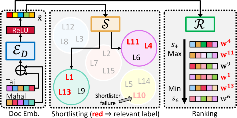
Figure 1. DECAF’s frugal prediction pipeline scales to millions of labels. Given a document ${\mathbf{x}}$, its text embedding $\hat{}{\mathbf{x}}$ (see Fig 3 (Left)) is first used by the shortlister ${\mathcal{S}}$ to shortlist the most probable ${\mathcal{O}}\left({{\log L}}\right)$ labels while maintaining high recall. The ranker ${\mathcal{R}}$ then uses label classifiers (see Fig 3 (Right)) of only the shortlisted labels to produce the final ranking.

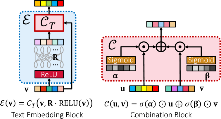
Figure 2. (Left) DECAF uses a lightweight architecture with a residual layer to embed both document and label text (see Fig. 3). (Right) Combination blocks are used to combine various representations (separate instances are used in the text embedding blocks (${\mathcal{E}}_{D},{\mathcal{E}}_{L}$) and in label classifiers (${\mathcal{C}}_{L}$)).

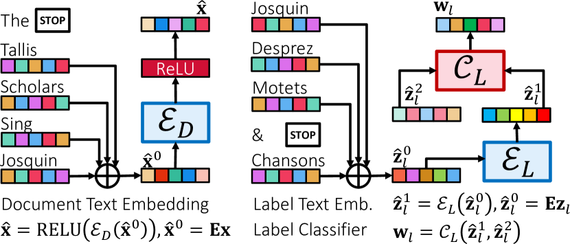
Figure 3. (Left) Document text is embedded using an instance ${\mathcal{E}}_{D}$ of the text embedding block (see Fig. 2). Stop words (e.g. and, the) are discarded. (Right) DECAF critically incorporates label text into classifier learning. For each label $l\in[L]$, a one-vs-all classifier ${\mathbf{w}}_{l}$ is learnt by combining label text embedding $\hat{}{\mathbf{z}}^{1}_{l}$ (using a separate instance ${\mathcal{E}}_{L}$ of the text embedding block) and a refinement vector $\hat{}{\mathbf{z}}^{2}_{l}$. Note that ${\mathcal{E}}_{D},{\mathcal{E}}_{L},{\mathcal{C}}_{L}$ use separate parameters. However, all labels share the blocks ${\mathcal{E}}_{L},{\mathcal{C}}_{L}$ and all documents share the block ${\mathcal{E}}_{D}$.

Summary: DECAF consists of three components 1) a lightweight text embedding block suitable for short-text applications, 2) 1-vs-All classifiers per label that incorporate label text, and 3) a shortlister that offers a high recall label shortlists for data points, allowing DECAF to offer sub-millisecond prediction times even with millions of labels. This section details these components, and an approximate likelihood model with provable recovery guarantees, using which DECAF offers a highly scalable yet accurate pipeline for jointly training text embeddings and classifier parameters.

Notation: Let $L$ be the number of labels and $V$ be the dictionary size. Each of the $N$ training points is presented as $({\mathbf{x}}_{i},{\mathbf{y}}_{i})$. ${\mathbf{x}}_{i}\in{\mathbb{R}}^{V}$ is a bag-of-tokens representation for the $i\text{${}^{\text{th}}$}$ document i.e. $x_{it}$ is the TF-IDF weight of token $t\in[V]$ in the $i\text{${}^{\text{th}}$}$ document. ${\mathbf{y}}_{i}\in\left\{{-1,+1}\right\}^{L}$ is the ground truth label vector with $y_{il}=+1$ if label $l\in[L]$ is relevant to the $i\text{${}^{\text{th}}$}$ document and $y_{il}=-1$ otherwise. For each label $l\in[L]$, its label text is similarly represented as ${\mathbf{z}}_{l}\in{\mathbb{R}}^{V}$.

Document and label-text embedding: DECAF learns $D$-dim embeddings for each vocabulary token i.e. ${\mathbf{E}}=\left[{{\mathbf{e}}_{1},\ldots,{\mathbf{e}}_{V}}\right]\in{\mathbb{R}}^{D\times V}$ and uses a light-weight embedding block (see Fig 3) to encode label and document texts. The embedding block ${\mathcal{E}}=\left\{{{\mathbf{R}},\text{\boldmath$\mathbf{\alpha}$},\text{\boldmath$\mathbf{\beta}$}}\right\}$ is parameterized by a residual block ${\mathbf{R}}\in{\mathbb{R}}^{d\times d}$ and scaling constants $\text{\boldmath$\mathbf{\alpha}$},\text{\boldmath$\mathbf{\beta}$}\in{\mathbb{R}}^{D}$ for the combination block (see Fig 2). The embedding for a bag-of-tokens vector, say ${\mathbf{r}}\in{\mathbb{R}}^{V}$, is ${\mathcal{E}}({\mathbf{r}})=\sigma(\text{\boldmath$\mathbf{\alpha}$})\odot\hat{}{\mathbf{r}}^{0}+\sigma(\text{\boldmath$\mathbf{\beta}$})\odot({\mathbf{R}}\cdot\text{ReLU}(\hat{}{\mathbf{r}}^{0}))\in{\mathbb{R}}^{D}$ where $\hat{}{\mathbf{r}}^{0}={\mathbf{E}}{\mathbf{r}}$, $\odot$ denotes component-wise multiplication, and $\sigma$ is the sigmoid function. Document embeddings, denoted by $\hat{}{\mathbf{x}}_{i}$, are computed as $\hat{}{\mathbf{x}}_{i}=\text{ReLU}({\mathcal{E}}_{D}({\mathbf{x}}_{i}))$. Label-text embeddings, denoted by $\hat{}{\mathbf{z}}^{1}_{l}$ are computed as $\hat{}{\mathbf{z}}^{1}_{l}={\mathcal{E}}_{L}({\mathbf{z}}_{l})$. Note that document and labels use separate instantiations ${\mathcal{E}}_{D},{\mathcal{E}}_{L}$ of the embedding block. We note that DECAF could also be made to use alternate text representations such as BERT (Devlin et al., 2019), attention (You et al., 2019), LSTM (Hochreiter and Schmidhuber, 1997) or convolution (Liu et al., 2017). However, such elaborate architectures negatively impact prediction time and moreover, DECAF outperforms BERT, CNN and attention based XML techniques on all our benchmark datasets indicating the suitability of DECAF’s frugal architecture to short-text applications.

1-vs-All Label Classifiers: DECAF uses high capacity 1-vs-All (OvA) classifiers ${\mathbf{W}}=[{\mathbf{w}}_{1},\ldots,{\mathbf{w}}_{L}]\in{\mathbb{R}}^{D\times L}$ that outperform tree- and embedding-based classifiers (Chang et al., 2020; Jain et al., 2019; Babbar and Schölkopf, 2019; Prabhu et al., 2018b; Yen et al., 2017; Babbar and Schölkopf, 2017). However, DECAF distinguishes itself from previous OvA works (even those such as (Chang et al., 2020) that do use label text) by directly incorporating label text into the OvA classifiers. For each label $l\in[L]$, the label-text embedding $\hat{}{\mathbf{z}}^{1}_{l}={\mathcal{E}}_{L}({\mathbf{z}}_{l})$ (see above) is combined with a refinement vector $\hat{}{\mathbf{z}}^{2}_{l}$ that is learnt separately per label, to produce the label classifier ${\mathbf{w}}_{l}=\sigma(\text{\boldmath$\mathbf{\alpha}$}_{L})\odot\hat{}{\mathbf{z}}^{1}_{l}+\sigma(\text{\boldmath$\mathbf{\beta}$}_{L})\odot\hat{}{\mathbf{z}}^{2}_{l}\in{\mathbb{R}}^{D}$ where $\text{\boldmath$\mathbf{\alpha}$}_{L},\text{\boldmath$\mathbf{\beta}$}_{L}\in{\mathbb{R}}^{D}$ are shared across labels (see Fig 3). Incorporating $\hat{}{\mathbf{z}}^{1}_{l}$ into the label classifier ${\mathbf{w}}_{l}$ allows labels that never co-occur, but nevertheless share tokens, to perform learning in a collaborative manner since if two labels, say $l,m\in[L]$ share some token $t\in[V]$ in their respective texts, then ${\mathbf{e}}_{t}$ contributes to both $\hat{}{\mathbf{z}}^{1}_{l}$ and $\hat{}{\mathbf{z}}^{1}_{m}$. In particular, this allows rare labels to share classifier information with popular labels with which they share a token. Ablation studies (Tab 4,5,6) show that incorporating label text into classifier learning offers DECAF significant gains of over 2-6% compared to methods that do not use label text. Incorporating other forms of label metadata, such as label hierarchies, could also lead to further gains.

Shortlister: OvA training and prediction can be prohibitive, $\Omega\left({{NDL}}\right)$ and $\Omega\left({{DL}}\right)$ resp., if done naively. A popular way to accelerate training is to, for every data point $i\in[N]$, use only a shortlist containing all positive labels (that are relatively fewer around ${\mathcal{O}}\left({{\log L}}\right)$) and a small subset of the, say again ${\mathcal{O}}\left({{\log L}}\right)$, most challenging negative labels (Chang et al., 2020; Jain et al., 2019; Khandagale et al., 2020; Prabhu et al., 2018b; Yen et al., 2017; Bhatia et al., 2015). This allows training to be performed in ${\mathcal{O}}\left({{ND\log L}}\right)$ time instead of ${\mathcal{O}}\left({{NDL}}\right)$ time. DECAF learns a shortlister ${\mathcal{S}}$ that offers a label-clustering based shortlisting. We have ${\mathcal{S}}=\left\{{{\mathcal{C}},{\mathbf{H}}}\right\}$ where ${\mathcal{C}}=\left\{{C_{1},\ldots,C_{K}}\right\}$ is a balanced clustering of the $L$ labels and ${\mathbf{H}}=[{\mathbf{h}}_{1},\ldots,{\mathbf{h}}_{K}]\in{\mathbb{R}}^{D\times K}$ are OvA classifiers, one for each cluster. Given the embedding $\hat{}{\mathbf{x}}$ of a document and beam-size $B$, the top $B$ clusters with the highest scores, say $\left\langle{{\mathbf{h}}_{m_{1}}},{\hat{}{\mathbf{x}}}\right\rangle\geq\left\langle{{\mathbf{h}}_{m_{2}}},{\hat{}{\mathbf{x}}}\right\rangle\geq\ldots$ are taken and labels present therein are shortlisted i.e. ${\mathcal{S}}(\hat{}{\mathbf{x}}):=\left\{{m_{1},\ldots,m_{B}}\right\}$. As clusters are balanced, we get, for every datapoint, $LB/K$ shortlisted labels in the clusters returned. DECAF uses $K=2^{17}$ clusters for large datasets.

Prediction Pipeline: Fig 1 shows the frugal prediction pipeline adopted by DECAF. Given a document ${\mathbf{x}}\in{\mathbb{R}}^{V}$, its embedding $\hat{}{\mathbf{x}}=\text{ReLU}({\mathcal{E}}_{D}({\mathbf{x}}))$ is used by the shortlister to obtain a shortlist of $B$ label clusters ${\mathcal{S}}(\hat{}{\mathbf{x}})=\left\{{m_{1},\ldots,m_{B}}\right\}$. Label scores are computed for every shortlisted label i.e. $l\in C_{m},m\in{\mathcal{S}}(\hat{}{\mathbf{x}})$ by combining shortlister and OvA classifier scores as $s_{l}:=\sigma(\left\langle{{\mathbf{w}}_{l}},{\hat{}{\mathbf{x}}}\right\rangle)\cdot\sigma(\left\langle{{\mathbf{h}}_{m}},{\hat{}{\mathbf{x}}}\right\rangle)$. These scores are sorted to make the final prediction. In practice, even on a dataset with 1.3 million labels, DECAF could make predictions within 0.2 ms using a GPU and 2 ms using a CPU.

3.1. Efficient Training: the DeepXML Pipeline

Summary: DECAF adopts the scalable DeepXML pipeline (Dahiya et al., 2021) that splits training into 4 modules. In summary, Module I jointly learns the token embeddings ${\mathbf{E}}$, the embedding modules ${\mathcal{E}}_{D},{\mathcal{E}}_{L}$ and shortlister ${\mathcal{S}}$. Module II fine-tunes ${\mathcal{E}}_{D},{\mathcal{E}}_{L},{\mathcal{S}}$, and retrieves label shortlists for all data points. After performing initialization in Module III, Module IV jointly learns the OvA classifiers ${\mathbf{W}}$ and fine-tunes ${\mathcal{E}}_{D},{\mathcal{E}}_{L}$ using the shortlists generated in Module II. Due to lack of space some details are provided in the supplementary material

Module I: Token embeddings ${\mathbf{E}}\in{\mathbb{R}}^{D\times V}$ are randomly initialized using (He et al., 2015), residual blocks within the blocks ${\mathcal{E}}_{D},{\mathcal{E}}_{L}$ are initialized to identity, and label centroids are created by aggregating document information for each label $l\in[L]$ as ${\mathbf{c}}_{l}=\sum_{i:y_{il}=+1}{\mathbf{x}}_{i}$. Balanced hierarchical binary clustering (Prabhu et al., 2018b) is now done on these label centroids for 17 levels to generate $K$ label clusters. Clustering labels using label centroids gave superior performance than using other representations such as label text ${\mathbf{z}}_{l}$. This is because the label centroid carries information from multiple documents and thus, a diverse set of tokens whereas ${\mathbf{z}}_{l}$ contains information from only a handful of tokens. The hierarchy itself is discarded and each resulting cluster is now treated as a meta-label that gives us a meta multi-label classification problem on the same training points, but with $K$ meta-labels instead of the original $L$ labels. Each meta label $m\in[K]$ is granted meta-label text as ${\mathbf{u}}_{m}=\sum_{l\in C_{m}}{\mathbf{z}}_{l}$. Each datapoint $i\in[N]$ is assigned a meta-label vector $\tilde{}{\mathbf{y}}_{i}\in\left\{{-1,+1}\right\}^{K}$ such that $\tilde{y}_{im}=+1$ if $y_{il}=+1$ for any $l\in C_{m}$ and $\tilde{y}_{im}=-1$ if $y_{il}=-1$ for all $l\in C_{m}$. OvA meta-classifiers ${\mathbf{H}}=[{\mathbf{h}}_{1},\ldots,{\mathbf{h}}_{K}]\in{\mathbb{R}}^{D\times K}$ are learnt to solve this meta multi-label problem but are constrained in Module I to be of the form ${\mathbf{h}}_{m}={\mathcal{E}}_{L}({\mathbf{u}}_{m})$. This constrained form of the meta-classifier forces good token embeddings ${\mathbf{E}}$ to be learnt that allow meta-classification without the assistance of powerful refinement vectors. However, this form continues to allow collaborative learning among meta classifiers based on shared tokens. Module I solves the meta multi-label classification problem while jointly training ${\mathcal{E}}_{D},{\mathcal{E}}_{L},{\mathbf{E}}$ (implicitly learning ${\mathbf{H}}$ in the process).

Module II: The shortlister is fine-tuned in this module. Label centroids are recomputed as ${\mathbf{c}}_{l}=\sum_{i:{\mathbf{y}}^{i}_{l}=+1}{\mathbf{E}}{\mathbf{x}}_{i}$ where ${\mathbf{E}}$ are the task-specific token embeddings learnt in Module I. The meta multi-label classification problem is recreated using these new centroids by following the same steps outlined in Module I. Module II uses OvA meta-classifiers that are more powerful and resemble those used by DECAF. Specifically, we now have ${\mathbf{h}}_{m}=\sigma(\tilde{\text{\boldmath$\mathbf{\alpha}$}}_{P})\odot\hat{}{\mathbf{u}}^{2}_{m}+\sigma(\tilde{\text{\boldmath$\mathbf{\beta}$}}_{P})\odot\hat{}{\mathbf{u}}^{1}_{m}$ where $\hat{}{\mathbf{u}}^{1}_{m}=\sum_{l\in C_{m}}{\mathcal{E}}_{L}({\mathbf{z}}_{l})$ is the meta label-text embedding, $\hat{}{\mathbf{u}}^{2}_{m}$ are meta label-specific refinement vectors, and ${\mathcal{C}}_{P}=\left\{{\tilde{\text{\boldmath$\mathbf{\alpha}$}}_{P},\tilde{\text{\boldmath$\mathbf{\beta}$}}_{P}}\right\}$ is a fresh instantiating of the combination block. Module II solves the (new) meta multi-label classification problem, jointly learning ${\mathcal{C}}_{P},\hat{}{\mathbf{u}}^{2}_{m}$ (implicitly updating ${\mathbf{H}}$ in the process) and fine-tuning ${\mathcal{E}}_{D},{\mathcal{E}}_{L},{\mathbf{E}}$. The shortlister ${\mathcal{S}}$ so learnt is now used to retrieve shortlists ${\mathcal{S}}({\mathbf{x}}_{i})$ for each data point $i\in[N]$.

Module III: Residual blocks within ${\mathcal{E}}_{D},{\mathcal{E}}_{L}$ are re-initialized to identity, ${\mathcal{S}}$ is frozen and combination block parameters for the OvA classifiers are initialized to $\text{\boldmath$\mathbf{\alpha}$}_{L}=\text{\boldmath$\mathbf{\beta}$}_{L}={\mathbf{0}}$ (note that $\sigma({\mathbf{0}})=0.5\cdot{\mathbf{1}}$ where ${\mathbf{1}}$ is the all-ones vector). Refinement vectors for all $L$ labels are initialized to $\hat{}{\mathbf{z}}^{2}_{l}={\mathbf{E}}{\mathbf{z}}_{l}$. Ablation studies (see Tab 6) show that this refinement vector initialization offers performance boosts of up to 5-10% compared to random initialization as is used by existing methods such as AttentionXML (You et al., 2019) and the X-Transformer (Chang et al., 2020).

Module IV: This module performs learning using an approximate likelihood model. Let $\Theta=\left\{{{\mathbf{E}},{\mathcal{E}}_{D},{\mathcal{E}}_{L},{\mathcal{C}}_{L},{\mathbf{W}}}\right\}$ be the model parameters in the DECAF architecture. We recall that ${\mathcal{C}}_{L}$ are combination blocks used to construct the OvA classifiers and meta classifiers, and ${\mathbf{E}}$ are the token embeddings. OvA approaches assume a likelihood decomposition such as ${\mathbb{P}}\left[{{{\mathbf{y}}_{i}\,|\,{\mathbf{x}}_{i},\Theta}}\right]=\prod_{l=1}^{L}{\mathbb{P}}\left[{{y_{il}\,|\,\hat{}{\mathbf{x}}_{i},{\mathbf{w}}_{l}}}\right]=\prod_{l=1}^{L}\left({1+\exp\left({-y_{il}\cdot\left\langle{\hat{}{\mathbf{x}}_{i}},{{\mathbf{w}}_{l}}\right\rangle}\right)}\right)^{-1}$. Here $\hat{}{\mathbf{x}}_{i}=\text{ReLU}({\mathcal{E}}_{D}({\mathbf{x}}_{i}))$ is the document-text embedding and ${\mathbf{w}}_{l}$ are the OvA classifiers as shown in Fig 3. Let us abbreviate $\ell_{il}(\Theta)=\ln\left({1+\exp\left({-y_{il}\cdot\left\langle{\hat{}{\mathbf{x}}_{i}},{{\mathbf{w}}_{l}}\right\rangle}\right)}\right)$. Then, our objective is to optimize $\mathop{\arg\min}_{\Theta}{\mathcal{L}}(\Theta)$ where

$${\mathcal{L}}(\Theta)=\frac{1}{NL}\sum_{i\in[N]}\sum_{l\in[L]}\ell_{il}(\Theta)$$

However, performing the above optimization exactly is intractable and takes $\Omega\left({{NDL}}\right)$ time. DECAF’s solves this problem by instead optimizing $\mathop{\arg\min}_{\Theta}\tilde{\mathcal{L}}(\Theta\,|\,{\mathcal{S}})$ where

$$\tilde{\mathcal{L}}(\Theta\,|\,{\mathcal{S}})=\frac{K}{NLB}\sum_{i\in[N]}\sum_{l\in{\mathcal{S}}(\hat{}{\mathbf{x}}_{i})}\ell_{il}(\Theta)$$

Recall that for any document, ${\mathcal{S}}(\hat{}{\mathbf{x}}_{i})$ is a shortlist of $B$ label clusters (that give us a total of $LB/K$ labels). Thus, the above expression contains only $NLB/K\ll NL$ terms as DECAF uses a large fanout of $K\approx 130$K and $B\approx 100$. The result below assures us that model parameters and embeddings obtained by optimizing $\tilde{\mathcal{L}}(\Theta\,|\,{\mathcal{S}})$ perform well w.r.t. the original likelihood ${\mathcal{L}}(\Theta)$ if the dataset exhibits label sparsity, and the shortlister assures high recall.

Theorem 3.1.

Suppose the training data has label sparsity at rate $s$ i.e. $\sum_{i\in[N]}\sum_{l\in[L]}{\mathbb{I}}\left\{{y_{il}=+1}\right\}=s\cdot NL$ and the shortlister offers a recall rate of $r$ on the training set i.e. $\sum_{i\in[N]}\sum_{l\in{\mathcal{S}}(\hat{}{\mathbf{x}}_{i})}{\mathbb{I}}\left\{{y_{il}=+1}\right\}=rs\cdot NL$. Then if $\hat{\Theta}$ is obtained by optimizing the approximate likelihood function $\tilde{\mathcal{L}}(\Theta\,|\,{\mathcal{S}})$, then the following always holds

$${\mathcal{L}}(\hat{\Theta})\leq\min_{\Theta}{\mathcal{L}}(\Theta)+{\mathcal{O}}\left({{s(1-r)\ln(1/(s(1-r)))}}\right).$$

Please refer to Appendix A.1 in the supplementary material for the proof. As $s\rightarrow 0$ and $r\rightarrow 1$, the excess error term vanishes at rate at least $\sqrt{s(1-r)}$. Our XML datasets do exhibit label sparsity at rate $s\approx 10^{-5}$ and Fig 6 shows that DECAF’s shortlister does offer high recall with small shortlists (80% recall with $\approx 50$-sized shortlist and 85% recall with $\approx 100$-sized shortlist). Since Thm 3.1 holds in the completely agnostic setting, it establishes the utility of learning when likelihood maximization is performed only on label shortlists with high-recall. Module IV uses these shortlists to jointly learn the $L$ OvA classifiers ${\mathbf{W}}$ and ${\mathcal{C}}_{L}$, as well as fine-tune the embedding blocks ${\mathcal{E}}_{D},{\mathcal{E}}_{L}$ and token embeddings ${\mathbf{E}}$.

Loss Function and Regularization: Modules I, II, IV use the logistic loss and the Adam (Kingma and Ba, 2014) optimizer to train the model parameters and various refinement vectors. Residual layers used in the text embedding blocks ${\mathcal{E}}_{D},{\mathcal{E}}_{L}$ were subjected to spectral regularization (Miyato et al., 2018). All ReLU layers were followed by a dropout layer with 50% drop-rate in Module-I and 20% for the rest of the modules.

Ensemble Learning: DECAF learns an inexpensive ensemble of 3 instances (see Figure 6). The three instances share Module I training to promote scalability i.e. they inherit the same token embeddings. However, they carry out training Module II onwards independently. Thus, the shortlister and embedding modules get fine-tuned for each instance.

Time Complexity: Appendix A.2 in the supplementary material presents time complexity analysis for the DECAF modules.

4. Experiments

Table 1. Results on publicly available short-text datasets. DECAF was found to be 2–6% more accurate, as well as an order of magnitude faster at prediction compared to other deep learning based approaches. Algorithms marked with a ‘-’ were unable to scale on the given dataset within available resources and timeout period. Prediction times for DECAF within parenthesis indicate those obtained on a CPU whereas those outside parentheses are times on a GPU.

Method	PSP@1	PSP@5	P@1	P@5	Prediction Time (ms)
LF-AmazonTitles-131K
DECAF	30.85	41.42	38.4	18.65	0.1 (1.15)
Astec	29.22	39.49	37.12	18.24	2.34
AttentionXML	23.97	32.57	32.25	15.61	5.19
MACH	24.97	34.72	33.49	16.45	0.23
X-Transformer	21.72	27.09	29.95	13.07	15.38
Siamese	13.3	13.36	13.81	5.81	0.2
Parabel	23.27	32.14	32.6	15.61	0.69
Bonsai	24.75	34.86	34.11	16.63	7.49
DiSMEC	25.86	36.97	35.14	17.24	5.53
PfastreXML	26.81	34.24	32.56	16.05	2.32
XT	22.37	31.64	31.41	15.48	9.12
Slice	23.08	31.89	30.43	14.84	1.58
AnneXML	19.23	32.26	30.05	16.02	0.11
LF-WikiSeeAlsoTitles-320K
DECAF	16.73	21.01	25.14	12.86	0.09 (0.97)
Astec	13.69	17.5	22.72	11.43	2.67
AttentionXML	9.45	11.73	17.56	8.52	7.08
MACH	9.68	12.53	18.06	8.99	0.52
X-Transformer	-	-	-	-	-
Siamese	10.1	9.59	10.69	4.51	0.17
Parabel	9.24	11.8	17.68	8.59	0.8
Bonsai	10.69	13.79	19.31	9.55	14.82
DiSMEC	10.56	14.82	19.12	9.87	11.02
PfastreXML	12.15	13.26	17.1	8.35	2.59
XT	8.99	11.82	17.04	8.6	12.86
Slice	11.24	15.2	18.55	9.68	1.85
AnneXML	7.24	11.75	16.3	8.84	0.13
LF-AmazonTitles-1.3M
DECAF	22.07	29.3	50.67	40.35	0.16 (1.73)
Astec	21.47	27.86	48.82	38.44	2.61
AttentionXML	15.97	22.54	45.04	36.25	29.53
MACH	9.32	13.26	35.68	28.35	2.09
X-Transformer	-	-	-	-	-
Siamese	-	-	-	-	-
Parabel	16.94	24.13	46.79	37.65	0.89
Bonsai	18.48	25.95	47.87	38.34	39.03
DiSMEC	-	-	-	-	-
PfastreXML	28.71	32.51	37.08	31.43	23.64
XT	13.67	19.06	40.6	32.01	5.94
Slice	13.8	18.89	34.8	27.71	1.45
AnneXML	15.42	21.91	47.79	36.91	0.12

Datasets: Experiments were conducted on product-to-product and related-webpage recommendation datasets. These were short-text tasks with only the product/webpage titles being used to perform prediction. Of these, LF-AmazonTitles-131K, LF-AmazonTitles-1.3M, and LF-WikiSeeAlsoTitles-320K are publicly available at The Extreme Classification Repository (Bhatia et al., 2016). Results are also reported on two proprietary product-to-product recommendation datasets (LF-P2PTitles-300K and LF-P2PTitles-2M) mined from click logs of the Bing search engine, where a pair of products was considered similar if the Jaccard index of the set of queries which led to a click on them was found to be more than a certain threshold. We also considered some datasets’ long text counterparts, namely LF-Amazon-131K and LF-WikiSeeAlso-320K, which contained the entire product/webpage descriptions. Note that LF-AmazonTitles-131K and LF-AmazonTitles-1.3M (as well as their long-text counterparts) are subsets of the standard AmazonTitles-670K and AmazonTitles-3M datasets respectively, and were created by restricting the label set to labels for which label-text was available. Please refer to Appendix A.3 and Table 7 in the supplementary material for dataset preparation details and dataset statistics.

Baseline algorithms: DECAF was compared to leading deep extreme classifiers including the X-Transformer (Chang et al., 2020), Astec (Dahiya et al., 2021), XT (Wydmuch et al., 2018), AttentionXML (You et al., 2019), and MACH (Medini et al., 2019), as well as standard extreme classifiers based on fixed or sparse BoW features including Bonsai (Khandagale et al., 2020), DiSMEC (Babbar and Schölkopf, 2017), Parabel (Prabhu et al., 2018b), AnnexML (Tagami, 2017). Slice (Jain et al., 2019). Slice was trained with fixed FastText (Bojanowski et al., 2017) features, while other methods used sparse BoW features. Unfortunately, GLaS (Guo et al., 2019) could not be included in the experiments as their code was not publicly available. Each baseline deep learning method was given a 12-core Intel Skylake 2.4 GHz machine with 4 Nvidia V100 GPUs. However, DECAF was offered a 6-core Intel Skylake 2.4 GHz machine with a single Nvidia V100 GPU. A training timeout of 1 week was set for every method. Please refer to Table 9 in the supplementary material for more details.

Table 2. Results on proprietary product-to-product (P2P) recommendation datasets. C@20 denotes label coverage offered by the top 20 predictions of each method. DECAF offers significantly better accuracies than all competing methods. Other methods such as AnnexML and DiSMEC did not scale with available resources within the timeout period.

Method	PSP@1	PSP@5	P@1	P@5	C@20
LF-P2PTitles-300K
DECAF	42.43	62.3	47.17	22.69	95.32
Astec	39.44	57.83	44.30	21.56	95.61
Parabel	37.26	55.32	43.14	20.99	95.59
PfastreXML	35.79	49.9	39.4	18.77	87.91
Slice	27.03	34.95	31.27	25.19	95.06
LF-P2PTitles-2M
DECAF	36.65	45.15	40.27	31.45	93.08
Astec	32.75	41	36.34	28.74	95.3
Parabel	30.21	38.46	35.26	28.06	92.82
PfastreXML	28.84	35.65	30.52	24.6	88.05
Slice	27.03	34.95	31.27	25.19	93.43

Evaluation: Standard extreme classification metrics (Babbar and Schölkopf, 2019; Prabhu and Varma, 2014; Prabhu et al., 2018b; You et al., 2019; Liu et al., 2017), namely Precision (P@$k$) and propensity scored precision (PSP@$k$) for $k=1,3,5$ were used and are detailed in Appendix A.4 in the supplementary material.

Hyperparameters: DECAF has two tuneable hyperparameters a) beam-width $B$ which determines the shortlist length $LB/K$ and b) token embedding dimension $D$. $B$ was chosen after concluding Module II training by setting a value that ensured a recall of $>85\%$ on the training set (note that choosing $B=K$ trivially ensures $100\%$ recall). Doing so did not require DECAF to re-train Module II yet ensured a high quality shortlisting. Token embedding dimension $D$ was kept at 512 for larger datasets to improve the network capacity for large output spaces. For the small dataset LF-AmazonTitles-131K, clusters size $K$ was kept at $2^{15}$ and for other datasets it was kept at $2^{17}$. All other hyperparameters including learning rate, number of epochs were set to their default values across all datasets. Please refer to Table 8 in the supplementary material for details.

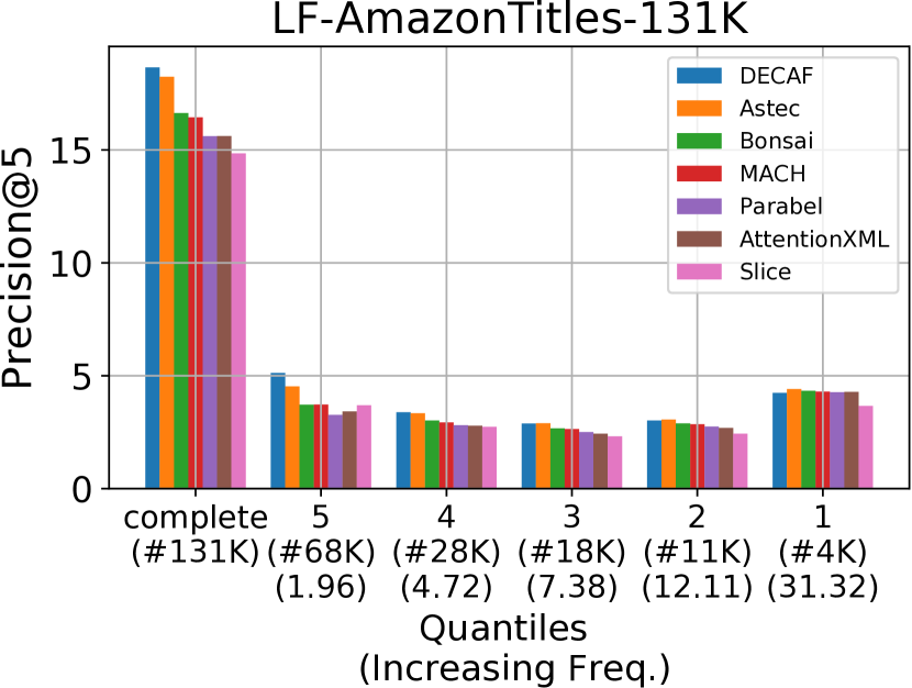
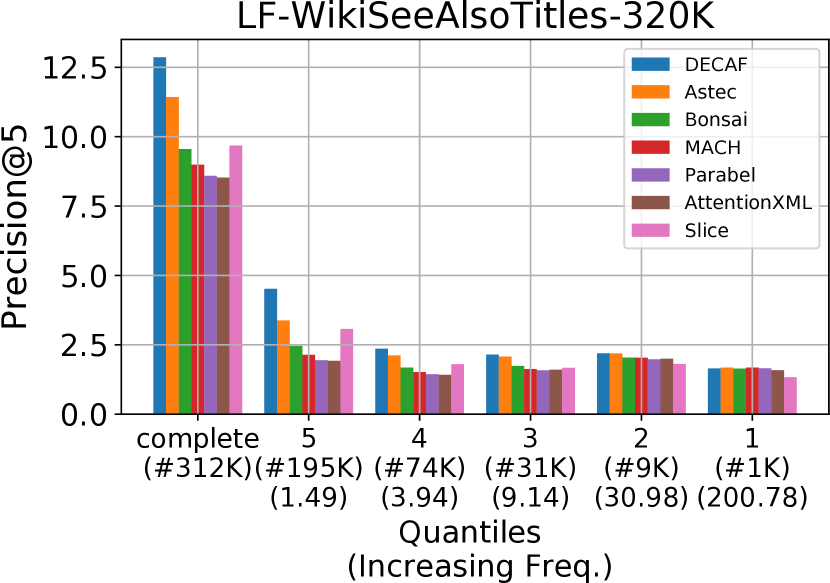
Figure 4. Quantile analysis of gains offered by DECAF in terms of contribution to P@5. The label set was divided into 5 equi-voluminous bins with increasing label frequency. Quantiles increase in mean label frequency from left to right. DECAF consistently outperforms other methods on all bins with the difference in accuracy being more prominent on bins containing data-scarce tail labels (e.g. bin 5).

Results on public datasets: Table 1 compares DECAF with leading XML algorithms on short-text product-to-product and related-webpage tasks. For details as well as results on long-text versions of these datasets, please refer to Table 9 in the supplementary material. Furthermore, although DECAF focuses on product-to-product applications, results on product-to-category style datasets such as product-to-category prediction on Amazon or article-to-category prediction on Wikipedia are reported in Table 10 in the supplementary material. Parabel (Prabhu et al., 2018a), Bonsai (Khandagale et al., 2020), AttentionXML (You et al., 2019) and X-Transformer (Chang et al., 2020) are the most relevant methods to DECAF as they shortlist labels based on a tree learned in the label centroid space. DECAF was found to be $4-10\%$ more accurate than methods such as Slice (Jain et al., 2019), PfastreXML (Jain et al., 2017), DiSMEC (Babbar and Schölkopf, 2017), and AnnexML (Tagami, 2017) that use fixed or pre-learnt features. This demonstrates that learning tasks-specific features can lead to significantly more accurate predictions. DECAF was also compared with other leading deep learning based approaches like MACH (Medini et al., 2019), and XT (Wydmuch et al., 2018). DECAF could be up to $7\%$ more accurate while being more than 150$\times$ faster at prediction as compared to attention based models like X-Transformer and AttentionXML. DECAF was also compared to Siamese networks that had similar access to label metadata as DECAF. However, DECAF could be up to $15\%$ more accurate than a Siamese network at an extreme scale. DECAF was also compared to Astec (Dahiya et al., 2021) that was specifically designed for short-text applications but does not utilize label metadata. DECAF could be up to 3% more accurate than Astec. This further supports DECAF’s claim of using label meta-data for improving prediction accuracy. Even on long-text tasks such as the LF-WikiSeeAlso-320K dataset (please refer to Table 9 in the supplementary material), DECAF can be more accurate in propensity scored metrics compared to the second best method AttentionXML, in addition to being vastly superior in terms of prediction time. This indicates the suitability of DECAF’s frugal architecture to product-to-product scenarios. The frugal architecture also allows DECAF to make predictions on a CPU within a few milliseconds even for large datasets such as LF-AmazonTitles-1.3M while other deep extreme classifiers can take an order of magnitude longer time even on a GPU. DECAF’s prediction times on a CPU are reported within parentheses in Table 1.

Results on proprietary datasets: Table 2 presents results on proprietary product-to-product recommendation tasks (with details presented in Table 11 in the supplementary material). DECAF could easily scale to the LF-P2PTitles-2M dataset and be upto 2% more accurate than leading XML algorithms including Bonsai, Slice and Parabel. Unfortunately, leading deep learning algorithms such as X-Transformer could not scale to this dataset within the timeout. DECAF offers label coverage similar to state-of-the-art XML methods yet offers the best accuracy in terms of P@1. Thus, DECAF’s superior predictions do not come at a cost of coverage.

Table 3. DECAF’s predictions on selected test points. Document and label names ending in “$\dots$” were abbreviated due to lack of space. Please refer to Table 12 in the supplementary material for the complete table. Predictions in black and a non-bold/non-italic font were a part of the ground truth. Those in bold italics were part of the ground truth but never seen with other the ground truth labels in the training set i.e. had no common training points. Predictions in light gray were not a part of the ground truth. DECAF’s exploits label metadata to discover semantically correlated labels.

Document	Top 5 predictions by DECAF
Panzer Dragoon Zwei	Panzer Dragoon, Action Replay Plus, Sega Saturn System - Video Game Console, The Legend of Dragoon , Panzer Dragoon Orta
Wagner - Die Walkure $\dots$	Wagner - Siegfried $\dots$, Wagner - Gotterdammerung $\dots$, Wagner - Der Fliegende Holländer (1986), Wagner - Gotterdammerung $\dots$, Seligpreisung
New Zealand dollar	Economy of New Zealand, Cook Islands dollar, Politics of New Zealand , Pitcairn Islands dollar, Australian dollar

Analysis: Table 3 shows specific examples of DECAF predictions. DECAF encourages collaborative learning among labels which allows it to predict the labels “Australian dollar" and “Economy of New Zealand” for the document “New Zealand dollar” when other methods failed to do so. This example was taken from the LF-WikiseeAlsoTitles-320K dataset (please refer to Table 12 in the supplementary material for details). It is notable that these labels do not share any common training instances with other ground truth labels but are semantically related nevertheless. DECAF similarly predicted a rare label “Panzer Dragoon Orta” for the (video game) product “Panzer Dragoon Zwei’ whereas other algorithms failed to do so. To better understand the nature of DECAF’s gains, the label set was divided into five uniform bins (quantiles) based on frequency of occurrence in the training set. DECAF’s collaborative approach using label text in classifier learning led to gains in every quantile, the gains were more prominent on the data-scarce tail-labels, as demonstrated in Figure 4.

Incorporating metadata into baseline XML algorithms: In principle, DECAF’s formulation could be deployed with existing XML algorithms wherever collaborative learning is feasible. Table 4 shows that introducing label text embeddings to the DiSMEC, Parabel, and Bonsai classifiers led to upto $1.5\%$ gain as compared to their vanilla counterparts that do not use label text. Details of these augmentations are given in Appendix A.5 in the supplementary material. Thus, label text inclusion can lead to gains for existing methods as well. However, DECAF continues to be upto $7\%$ more accurate than even these augmented versions. This shows that DECAF is more efficient at utilizing available label text.

Table 4. Augmenting existing BoW-based XML methods by incorporating label metadata leads to $1.5\%$ increase in the accuracy as compared to base method. However, DECAF could be up to $7\%$ more accurate compared to even these.

Method	PSP@1	PSP@5	P@1	P@5
LF-AmazonTitles-131K
DECAF	30.85	41.42	38.4	18.65
Parabel	23.27	32.14	32.6	15.61
Parabel + metadata	25.89	34.83	33.6	15.84
Bonsai	24.75	34.86	34.11	16.63
Bonsai + metadata	26.82	36.63	34.83	16.67
DiSMEC	26.25	37.15	35.14	17.24
DiSMEC + metadata	27.19	38.17	35.52	17.52
LF-WikiSeeAlsoTitles-320K
DECAF	16.73	21.01	25.14	12.86
Parabel	9.24	11.8	17.68	8.59
Parabel + metadata	12.96	16.77	20.69	10.24
Bonsai	10.69	13.79	19.31	9.55
Bonsai + metadata	13.63	17.54	21.61	10.72
DiSMEC	10.56	14.82	19.12	9.87
DiSMEC + metadata	12.46	15.9	20.74	10.29

Table 5. Using strategies used by existing XML algorithms for shortlisting labels instead of ${\mathcal{S}}$ hurts both both shortlist recall (R@20) and final prediction accuracy (P@k, PSP@k).

Method	PSP@1	PSP@5	P@1	P@5	R@20
LF-AmazonTitles-131K
DECAF	30.85	41.42	38.4	18.65	55.86
+ HNSW Shortlist	29.55	39.17	36.7	17.78	48.82
+ Parabel Shortlist	24.88	31.21	32.13	14.73	39.36
LF-WikiSeeAlsoTitles-320K
DECAF	16.73	21.01	25.14	12.86	37.53
+ HNSW Shortlist	15.68	19.38	23.84	12.11	30.26
+ Parabel Shortlist	13.17	15.09	21.18	10.05	23.91

Table 6. Analyzing the impact for alternative design and algorithmic choices for DECAF’s components.

Component	PSP@1	PSP@5	P@1	P@5	R@20
LF-AmazonTitles-131K
DECAF	30.85	41.42	38.4	18.65	55.86
DECAF-FFT	25.5	33.38	32.42	15.43	47.23
DECAF-8K	29.07	38.7	36.29	17.52	51.65
DECAF-no-init	29.86	41.04	37.79	18.57	55.75
DECAF-$\hat{}{\mathbf{z}}^{1}$	28.02	38.38	33.5	17.09	53.83
DECAF-$\hat{}{\mathbf{z}}^{2}$	27.32	38.05	36	17.65	52.2
DECAF-lite	29.75	40.36	37.26	18.29	55.25
LF-WikiSeeAlsoTitles-320K
DECAF	16.73	21.01	25.14	12.86	37.53
DECAF-FFT	13.91	17.3	21.72	11	32.58
DECAF-8K	14.55	17.38	22.41	10.96	30.21
DECAF-no-init	15.09	19.47	23.81	12.25	36.18
DECAF-$\hat{}{\mathbf{z}}^{1}$	18.04	21.48	24.54	12.55	37.33
DECAF-$\hat{}{\mathbf{z}}^{2}$	11.55	15.24	20.82	10.53	29.72
DECAF-lite	16.59	20.84	24.87	12.78	37.24

Figure 5. Impact of the number of instances in DECAF’s ensemble on performance on the LF-AmazonTitles-131K dataset. DECAF offers maximum benefits using a small ensemble of 3 instances after which benefits taper off.

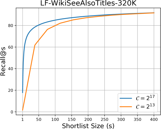
Figure 6. A comparison of recall when using moderate or large fanout on the LF-WikiSeeAlso-320K dataset. The x-axis represents various values of beam-width $B$ and training recall offered by each. A large fanout offers superior recall with small beam width, and hence small shortlists lengths.

Shortlister: DECAF’s shortlister distinguishes itself from previous shortlisting strategies (Chang et al., 2020; Khandagale et al., 2020; You et al., 2019; Prabhu et al., 2018b) in two critical ways. Firstly, DECAF uses a massive fanout of $K=2^{17}\approx 130$K clusters whereas existing approaches either use much fewer (upto 8K) clusters (Chang et al., 2020; Bhatia et al., 2015) or use hierarchical clustering with a small fanout (upto 100) at each node (Khandagale et al., 2020; You et al., 2019). Secondly, in contrast to other methods that create shortlists from generic embeddings (e.g. bag-of-words or FastText (Joulin et al., 2017)), DECAF fine-tunes its shortlister in Module II using task-specific embeddings learnt in Module I. Tables 5 and 6 show that DECAF’s shortlister offers much better performance than shortlists computed using a small fanout or else computed using ANNS-based negative sampling (Jain et al., 2019). Fig 6 shows that a large fanout offers much better recall even with small shortlist lengths than if using even moderate fanouts e.g. $K=8$K.

Ablation: As described in Section 3, the training pipeline for DECAF is divided into 4 modules mirroring the DeepXML pipeline (Dahiya et al., 2021). Table 6 presents the results of extensive experiments conducted to analyze the optimality of algorithmic and design choices made in these modules. We refer to Appendix A.5 in the supplementary material for details. a) To assess the utility of learning task-specific token embeddings in Module I, a variant DECAF-FFT was devised that replaced these with pre-trained FastText embeddings: DECAF outperforms DECAF-FFT by 6% in PSP@1 and 3.5% in P@1. b) To assess the impact of a large fanout while learning the shortlister, a variant DECAF-8K was trained with a smaller fanout of $K=2^{13}\approx 8$K clusters that is used by methods such as AttentionXML and X-Transformer. Restricting fanout was found to hurt accuracy by 3%. This can be attributed to the fact that the classifier’s final accuracy depends on the recall of the shortlister (see Theorem 3.1). Fig. 6 indicates that using $K=2^{13}$ results in significantly larger shortlist lengths (upto $2\times$ larger) being required to achieve the same recall as compared to using $K=2^{17}$. Large shortlists make Module IV training and prediction more challenging, especially for large datasets involving millions of labels, thereby making a large fan-out $K$ more beneficial. c) Approaches other than DECAF’s shortlister ${\mathcal{S}}$ were considered for shortlisting labels, such as nearest neighbor search using HNSW (Jain et al., 2019) or PLTs with small fanout such as Parabel (Prabhu et al., 2018b) learnt over dense document embeddings. Table 5 shows that both alternatives lead to significant loss, upto 15% in recall, as compared to that offered by ${\mathcal{S}}$. These sub-optimal shortlists eventually hurt final prediction which could be 2% less accurate as compared to DECAF. d) To assess the importance of label classifier initialization in Module III, a variant DECAF-no-init was tested which initialized $\hat{}{\mathbf{z}}^{2}_{l}$ randomly instead of with ${\mathbf{E}}{\mathbf{z}}_{l}$. DECAF-no-init was found to offer 1-1.5% less PSP@1 than DECAF, therefore indicating importance of proper initialization in Module III. e) Modules II and IV learn OvA classifiers as a combination of the label embedding vector and a refinement vector. To investigate the need for both components, Table 6 considers two DECAF variants: the first variant, named DECAF-$\hat{}{\mathbf{z}}^{1}$, discards the refinement vector in both modules i.e. using ${\mathbf{w}}_{l}=\hat{}{\mathbf{z}}^{1}_{l}$ and ${\mathbf{h}}_{m}=\hat{}{\mathbf{u}}^{1}_{m}$ whereas the second variant, named DECAF-$\hat{}{\mathbf{z}}^{2}$, rejects the label embedding component altogether and learns the OvA classifers from scratch using only the refinement vector i.e. using ${\mathbf{w}}_{l}=\hat{}{\mathbf{z}}^{2}_{l}$ and ${\mathbf{h}}_{m}=\hat{}{\mathbf{u}}^{2}_{m}$. Both variants take a hit of up to 5% in prediction accuracy as compared to DECAF. Incorporating label-text in the classifier is critical to achieve superior accuracies. f) Finally, to assess the utility of fine-tuning token embeddings in each successive module, a frugal version DECAF-lite was considered which freezes token embeddings after Module I and shares token embeddings among the three instances in its ensemble. DECAF-lite offers 0.5-1% loss in performance as compared to DECAF but is noticeably faster at training.

5. Conclusion

This paper demonstrated the impact of incorporating label metadata in the form of label text in offering significant performance gains on several product-to-product recommendation tasks. It proposed the DECAF algorithm that uses a frugal architecture, as well as a scalable prediction pipeline, to offer predictions that are up to 2-6% more accurate, as well as an order of magnitude faster, as compared to leading deep learning-based XML algorithms. DECAF offers millisecond-level prediction times on a CPU making it suitable for real-time applications such as product-to-product recommendation tasks. Future directions of work include incorporating other forms of label metadata such as label-correlation graphs, as well as diverse embedding architectures.

Appendix A Appendix

In this supplementary material, we present various details omitted from the main text due to lack of space, including a proof of Thm 3.1, a detailed analysis of the time complexity of the various modules in the training and prediction pipelines of DECAF, details of the datasets and evaluation metrics used in the experiments, further clarifications about how some ablation experiments were carried out, as well as additional experimental results including a subjective comparison of the prediction quality of DECAF and various competitors on handpicked recommendation examples.

A.1. Proof of Theorem 3.1

We recall from the main text that ${\mathcal{L}}(\Theta)$ denotes the original likelihood expression and $\tilde{\mathcal{L}}(\Theta\,|\,{\mathcal{S}})$ denotes the approximate likelihood expression that incorporates the shortlister ${\mathcal{S}}$. Both expression are reproduced below for sake of clarity.

$${\mathcal{L}}(\Theta) =\frac{1}{NL}\sum_{i\in[N]}\sum_{l\in[L]}\ell_{il}(\Theta)$$

$$\tilde{\mathcal{L}}(\Theta\,|\,{\mathcal{S}}) =\frac{K}{NLB}\sum_{i\in[N]}\sum_{l\in{\mathcal{S}}(\hat{}{\mathbf{x}}_{i})}\ell_{il}(\Theta)$$

Theorem A.1 (Theorem 3.1 Restated).

Suppose the training data has label sparsity at rate $s$ i.e. $\sum_{i\in[N]}\sum_{l\in[L]}{\mathbb{I}}\left\{{y_{il}=+1}\right\}=s\cdot NL$ and the shortlister offers a recall rate of $r$ on the training set i.e. $\sum_{i\in[N]}\sum_{l\in{\mathcal{S}}(\hat{}{\mathbf{x}}_{i})}{\mathbb{I}}\left\{{y_{il}=+1}\right\}=rs\cdot NL$. Then if $\hat{\Theta}$ is obtained by optimizing the approximate likelihood function $\tilde{\mathcal{L}}(\Theta\,|\,{\mathcal{S}})$, then the following always holds

$${\mathcal{L}}(\hat{\Theta})\leq\min_{\Theta}{\mathcal{L}}(\Theta)+{\mathcal{O}}\left({{s(1-r)\ln\left({\frac{1}{s(1-r)}}\right)}}\right).$$

Below we prove the above claimed result. For the sake of simplicity, let $\Theta^{\ast}=\mathop{\arg\min}_{\Theta}\ {\mathcal{L}}(\Theta)$ denote the optimal model that could have been learnt using the original likelihood expression. As discussed in Sec 3, OvA methods with linear classifiers assume a likelihood decomposition of the form ${\mathbb{P}}\left[{{{\mathbf{y}}_{i}\,|\,{\mathbf{x}}_{i},\Theta}}\right]=\prod_{l=1}^{L}{\mathbb{P}}\left[{{y_{il}\,|\,\hat{}{\mathbf{x}}_{i},{\mathbf{w}}_{l}}}\right]=\prod_{l=1}^{L}\left({1+\exp\left({y_{il}\cdot\left\langle{\hat{}{\mathbf{x}}_{i}},{{\mathbf{w}}_{l}}\right\rangle}\right)}\right)^{-1}$ where $\hat{}{\mathbf{x}}_{i}=\text{ReLU}({\mathcal{E}}({\mathbf{x}}_{i}))$ is the document embedding obtained using token embeddings ${\mathbf{E}}$ and embedding block parameters taken from $\Theta$, and ${\mathbf{w}}_{l}$ is the label classifier obtained as shown in Fig 3. Thus, for a label-document pair $(i,l)\in[N]\times[L]$, the model posits a likelihood

$${\mathbb{P}}\left[{{y_{il}\,|\,\hat{}{\mathbf{x}}_{i},{\mathbf{w}}_{l}}}\right]=\left({1+\exp\left({y_{il}\cdot\left\langle{\hat{}{\mathbf{x}}_{i}},{{\mathbf{w}}_{l}}\right\rangle}\right)}\right)^{-1}$$

However, in the presence of a shortlister ${\mathcal{S}}$, the above model fails to hold since for a document $i$, a label $l\notin{\mathcal{S}}(\hat{}{\mathbf{x}}_{i})$ is never predicted. This can cause a catastrophic collapse of the model likelihood if even a single positive label fails to be shortlisted by the shortlister, i.e. if the shortlister admits even a single false negative. To address this, and allow DECAF to continue working with shortlisters with high but still imperfect recall, we augment the likelihood model as follows

$${\mathbb{P}}\left[{{y_{il}\,|\,\hat{}{\mathbf{x}}_{i},{\mathbf{w}}_{l}}}\right]=\begin{cases}\left({1+\exp\left({y_{il}\cdot\left\langle{\hat{}{\mathbf{x}}_{i}},{{\mathbf{w}}_{l}}\right\rangle}\right)}\right)^{-1}&l\in{\mathcal{S}}(\hat{}{\mathbf{x}}_{i})\\ y_{il}\left({\eta-\frac{1}{2}}\right)+\frac{1}{2}&l\notin{\mathcal{S}}(\hat{}{\mathbf{x}}_{i})\end{cases},$$

where $\eta\in(0,1]$ is some default likelihood value assigned to positive labels that escape shortlisting (recall that $y_{il}\in\left\{{-1,+1}\right\}$). Essentially, for non-shortlisted labels, we posit their probability of being relevant as $\eta$. The value of $\eta$ will be tuned later.

Note that we must set $\eta\ll 1$ so as to ensure that these default likelihood scores do not interfere with the prediction pipeline which discards non-shortlisted labels. We will see that our calculations do result in an extremely small value of $\eta$ as the optimal value. However, also note that we cannot simply set $\eta=0$ since that would lead to a catastrophic collapse of the model likelihood to zero if the shortlister has even one false negative. Although our shortlister does offer good recall even with shortists of small length (e.g. 85% with a shortlist of length $\approx 200$), demanding 100% recall would require exorbitantly large beam sizes that would slow down prediction greatly. Thus, it is imperative that the augmented likelihood model itself account for shortlister failures.

To incorporate the above augmentation, we also redefine our log-likelihood score function to handle document-label pairs $(i,l)\in[N]\times[L]$ such that $l\notin{\mathcal{S}}(\hat{}{\mathbf{x}}_{i})$

$$\ell_{il}(\Theta\,|\,{\mathcal{S}})=\begin{cases}\ln\left({1+\exp\left({y_{il}\cdot\left\langle{\hat{}{\mathbf{x}}_{i}},{{\mathbf{w}}_{l}}\right\rangle}\right)}\right)&l\in{\mathcal{S}}(\hat{}{\mathbf{x}}_{i})\\ -\ln\left({y_{il}\left({\eta-\frac{1}{2}}\right)+\frac{1}{2}}\right)&l\notin{\mathcal{S}}(\hat{}{\mathbf{x}}_{i})\end{cases},$$

Note the negative sign in the second case since $\ell_{ij}$ is the negative log-likelihood expression. We will also benefit from defining the following residual loss term

$$\Delta(\Theta\,|\,{\mathcal{S}})=\sum_{i\in[N]}\sum_{l\notin{\mathcal{S}}(\hat{}{\mathbf{x}}_{i})}\ell_{il}(\Theta)$$

Note that $\Delta$ simply sums up loss terms corresponding to all labels omitted by the shortlister. We will establish the result claimed in the theorem by comparing the performance offered by $\hat{\Theta}$ and $\Theta^{\ast}$ on the loss terms given by $\tilde{\mathcal{L}}$ and $\Delta$. Note that for any $\Theta$ we always have the following decomposition

$${\mathcal{L}}(\Theta)=\frac{1}{NL}\left({\frac{NLB}{K}\cdot\tilde{\mathcal{L}}(\Theta\,|\,{\mathcal{S}})+\Delta(\Theta\,|\,{\mathcal{S}}}\right)$$

Now, since $\hat{\Theta}$ optimizes $\tilde{\mathcal{L}}$, we have $\tilde{\mathcal{L}}(\hat{\Theta}\,|\,{\mathcal{S}})\leq\tilde{\mathcal{L}}(\Theta^{\ast}\,|\,{\mathcal{S}})$ which settles the first term in the above decomposition. To settle the second term, we note that as per the recall $r$ and label sparsity $s$ terms defined in the statement of the theorem, the number of positive labels not shortlisted by the shortlister ${\mathcal{S}}$ throughout the dataset is $\text{FPR}\cdot NL$ where $\text{FPR}=(1-r)s$ is the false negative rate of the shortlister. Similarly, the number of negative labels not shortlisted by the shortlister throughout the dataset by $(L-B)N$ can be seen to be $\text{TNR}\cdot NL$ where $\text{TNR}=\left({(1-s)-\frac{B}{K}+rs}\right)$ is the true negative rate of the shortlister. This gives us

$$\Delta(\hat{\Theta}\,|\,{\mathcal{S}})=\left({\text{FPR}\cdot\ln\frac{1}{\eta}+\text{TNR}\cdot\ln\frac{1}{1-\eta}}\right)\cdot NL$$

It is easy to see that the optimal value of $\eta$ for the above expression is $\eta=\frac{\text{FPR}}{\text{FPR}+\text{TNR}}$. For example, in the LF-WikiSeeAlsoTitles-320K dataset, which has $s\approx 6.75\times 10^{-6},r\approx 0.85,B=160,K=2^{17}$, this gives a value of $\text{FPR}\approx 1.01\times 10^{-6},\text{TNR}\approx 0.999$ which gives $\eta\approx 1.01\times 10^{-6}$. This confirms that the augmentation indeed does not interfere with the prediction pipeline and labels not shortlisted can be safely ignored. However, moving on and plugging this optimal value of $\eta$ into the expression tells us that

$$\Delta(\hat{\Theta}\,|\,{\mathcal{S}})=\left({\frac{\text{FPR}}{\text{TNR}}\ln\left({1+\frac{\text{TNR}}{\text{FPR}}}\right)+\ln\left({1+\frac{\text{FPR}}{\text{TNR}}}\right)}\right)\cdot NL.$$

Since $\text{TNR}\rightarrow 1$ (for example, we saw $\text{TNR}\approx 0.999$ above), we simplify this to $\frac{\text{FPR}}{\text{TNR}}={\mathcal{O}}\left({{\text{FPR}}}\right)$ and use the inequality $\ln(1+v)\leq v$ for all $v>0$ to conclude that $\Delta(\hat{\Theta}\,|\,{\mathcal{S}})\leq{\mathcal{O}}\left({{\text{FPR}\ln\frac{1}{\text{FPR}}+\text{FPR}}}\right)={\mathcal{O}}\left({{s(1-r)\ln\left({\frac{1}{s(1-r)}}\right)}}\right)$. Using $\Delta(\Theta^{\ast}\,|\,{\mathcal{S}})\geq 0$ settles the second term in the decomposition by establishing that $\Delta(\hat{\Theta}\,|\,{\mathcal{S}})-\Delta(\Theta^{\ast}\,|\,{\mathcal{S}})\leq{\mathcal{O}}\left({{s(1-r)\ln\left({\frac{1}{s(1-r)}}\right)}}\right)\cdot NL$. Combining the two terms in the decomposition above gives us

$${\mathcal{L}}(\hat{\Theta})-{\mathcal{L}}(\Theta^{\ast})=\frac{1}{NL}\left({\frac{NLB}{K}\cdot(\tilde{\mathcal{L}}(\Theta\,|\,{\mathcal{S}})-\tilde{\mathcal{L}}(\Theta^{\ast}\,|\,{\mathcal{S}}))+(\Delta(\Theta\,|\,{\mathcal{S}})-\Delta(\Theta^{\ast}\,|\,{\mathcal{S}}))}\right)\leq{\mathcal{O}}\left({{s(1-r)\ln\left({\frac{1}{s(1-r)}}\right)}}\right),$$

which finishes the proof of the theorem.

We conclude this discussion by noting that since ${\mathcal{L}}$ and $\tilde{\mathcal{L}}$ are non-convex objectives due to the non-linear architecture encoded by the model parameters $\Theta$, it may not be able to solve these objectives optimally in practice. Thus, in practice, all we may be ensure is that

$$\tilde{\mathcal{L}}(\hat{\Theta}\,|\,{\mathcal{S}})\leq\min_{\Theta}\tilde{\mathcal{L}}(\Theta\,|\,{\mathcal{S}})+\epsilon_{\text{opt}}$$

where $\epsilon_{\text{opt}}$ is the sub-optimality in optimizing the objective $\tilde{\mathcal{L}}$ due to factors such as sub-optimal initialization, training, premature termination, etc. It is easy to see that the main result of the theorem continues to hold since we now have $\tilde{\mathcal{L}}(\hat{\Theta}\,|\,{\mathcal{S}})\leq\tilde{\mathcal{L}}(\Theta^{\ast}\,|\,{\mathcal{S}})+\epsilon_{\text{opt}}$ which gives us the modified result as follows

$${\mathcal{L}}(\hat{\Theta})\leq\min_{\Theta}{\mathcal{L}}(\Theta)+{\mathcal{O}}\left({{s(1-r)\ln\left({\frac{1}{s(1-r)}}\right)}}\right)+\frac{B}{K}\epsilon_{\text{opt}}.$$

A.2. Time Complexity Analysis for DECAF

In this section, we discuss the time complexity of the various modules in DECAF, as well as derive the prediction and training complexities.

Notation: Recall from Section 3 that DECAF learns $D$-dimensional representations for all $V$ tokens (${\mathbf{e}}_{t},t\in[V]$), that are used to create embeddings for all $L$ labels $\hat{}{\mathbf{z}}^{1}_{l},l\in[L]$, and all $N$ training documents $\hat{}{\mathbf{x}}_{i},i\in[N]$. We introduce some additional notation to facilitate the discussion: we use $\hat{V}_{x}$ to denote the average number of unique tokens present in a document i.e. $\hat{V}_{x}=\frac{1}{N}\sum_{i=1}^{N}\left\|{{\mathbf{x}}_{i}}\right\|_{0}$ where $\left\|{\cdot}\right\|_{0}$ is the sparsity “norm” that gives the number of non-zero elements in a vector. We similarly use $\hat{V}_{y}=\frac{1}{L}\sum_{l=1}^{L}\left\|{{\mathbf{z}}_{l}}\right\|_{0}$ to denote the average number of tokens in a label text. Let $\hat{L}=\frac{1}{N}\sum_{i=1}^{N}\left\|{{\mathbf{y}}_{i}}\right\|_{0}$ denote the average number of labels per document and also let $\hat{N}=\frac{N\hat{L}}{L}$ denote the average number of documents per label. We also let $M$ denote the mini-batch size (DECAF used $M=255$ for all datasets – see Table 8).

Embedding Block: Given a text with $\hat{V}$ tokens, the embedding block requires $\hat{V}D$ operations to aggregate token embeddings and $D^{2}+3D$ operations to execute the residual block and the combination block, for a total of ${\mathcal{O}}\left({{\hat{V}D+D^{2}}}\right)$ operations. Thus, to encode a label (respectively document) text, it takes ${\mathcal{O}}\left({{\hat{V}_{y}D+D^{2}}}\right)$ (respectively ${\mathcal{O}}\left({{\hat{V}_{x}D+D^{2}}}\right)$) operations on average.

Prediction: Given a test document, assuming that it contain $\hat{V}_{x}$ tokens, embedding takes ${\mathcal{O}}\left({{\hat{V}_{x}D+D^{2}}}\right)$ operations, executing the shortlister by identifying the top $B$ clusters takes ${\mathcal{O}}\left({{KD+K\log K}}\right)$ operations. These clusters contain a total of $\frac{LB}{K}$ labels. The ranker takes ${\mathcal{O}}\left({{\frac{LB}{K}D+\frac{LB}{K}\log\left({\frac{LB}{K}}\right)}}\right)$ operations to execute the $\frac{LB}{K}$ OvA linear models corresponding to these shortlisted labels to obtain the top-ranked predictions. Thus, prediction takes ${\mathcal{O}}\left({{\hat{V}_{x}D+D^{2}+KD+K\log K}}\right)={\mathcal{O}}\left({{KD}}\right)$ time since usually $\frac{LB}{K}\leq K,\hat{V}_{x}\leq K$ and $\log K\leq D\leq K$.

Module I Training: Creation of all $L$ label centroids ${\mathbf{c}}_{l}$ takes ${\mathcal{O}}\left({{L\hat{N}\hat{V}_{x}}}\right)$ time. These centroids are ${\mathcal{O}}\left({{\hat{N}\hat{V}_{x}}}\right)$-sparse on average. Clustering these labels using hierarchical balanced binary clustering for $\log K$ levels to get $K$ balanced clusters takes time ${\mathcal{O}}\left({{L\hat{N}\hat{V}_{x}\log K}}\right)$. Computing meta label text representations ${\mathbf{u}}_{m}$ for all meta labels takes ${\mathcal{O}}\left({{L\hat{V}_{y}}}\right)$ time. The vectors ${\mathbf{u}}_{m}$ are $\frac{\hat{V}_{y}L}{K}$-sparse on average. To compute the complexity of learning the $K$ OvA meta-classifiers, we calculate below the cost of a single back-propagation step when using a mini-batch of size $M$. Computing the document and meta-label features of all $M$ documents in the mini-batch and $K$ meta-labels takes on average ${\mathcal{O}}\left({{(D^{2}+\hat{V}_{x}D)M}}\right)$ and ${\mathcal{O}}\left({{\left({D^{2}+\frac{\hat{V}_{y}L}{K}\cdot D}\right)K}}\right)$ time respectively. Computing the scores for all the OvA meta classifiers for all documents in the mini-batch takes ${\mathcal{O}}\left({{MKD}}\right)$ time. Overestimating that the $K$ meta label texts together cover all $V$ tokens, updating the residual layer parameters ${\mathbf{R}}$, the combination block parameters, and the token embeddings ${\mathbf{E}}$ using back-propagation takes at most ${\mathcal{O}}\left({{(D^{2}+V)MK}}\right)$ time.

Module II Training: Recreating all $L$ label centroids ${\mathbf{c}}_{l}$ now takes ${\mathcal{O}}\left({{L\hat{N}\hat{V}_{x}D}}\right)$ time. Clustering the labels takes time ${\mathcal{O}}\left({{LD\log K}}\right)$. Computing document features in a mini-batch of size $M$ takes ${\mathcal{O}}\left({{(\hat{V}_{x}D+D^{2})M}}\right)$ time as before. Computing the meta-label representations $\hat{}{\mathbf{u}}^{1}_{m}$ for all $K$ meta-labels now takes ${\mathcal{O}}\left({{(\hat{V}_{y}D+D^{2})L}}\right)$ time. Computing the scores for all the OvA meta classifiers for all documents in the mini-batch takes ${\mathcal{O}}\left({{MKD}}\right)$ time as before. Next, updating the model parameters as well as the refinement vectors $\hat{}{\mathbf{u}}^{2}_{m},m\in[K]$ takes at most ${\mathcal{O}}\left({{(D^{2}+V)MK}}\right)$ time time as before. The added task of updating $\hat{}{\mathbf{u}}^{2}_{m}$ does not affect the asymptotic complexity of this module. Generating the shortlists for all $N$ training points is essentially a prediction step and takes ${\mathcal{O}}\left({{NKD}}\right)$ time.

Module II Initializations: Model parameter initializations take ${\mathcal{O}}\left({{D^{2}}}\right)$ time. Initializing the refinement vectors $\hat{}{\mathbf{z}}^{2}_{l}$ takes ${\mathcal{O}}\left({{L\hat{V}_{y}D}}\right)$ time.

Module IV Training: Given the shortlist of $LB/K$ labels per training point generated in Module II, training the OvA classifiers by fine-tuning the model parameters and learning the refinement vectors $\hat{}{\mathbf{z}}^{2}_{l},l\in[L]$ is made much less expensive than ${\mathcal{O}}\left({{NLD}}\right)$. Computing document features in a mini-batch of size $M$ takes ${\mathcal{O}}\left({{(\hat{V}_{x}D+D^{2})M}}\right)$ time as before. However, label representations $\hat{}{\mathbf{z}}^{1}_{l}$ of only shortlisted labels need be computed. Since there are atmost $\left({\frac{LB}{K}+\hat{L}}\right)M$ of them (accounting for hard negatives and all positives), this takes ${\mathcal{O}}\left({{(\hat{V}_{y}D+D^{2})M\left({\frac{LB}{K}+\hat{L}}\right)}}\right)$ time. Next, updating the model parameters as well as the refinement vectors $\hat{}{\mathbf{z}}^{2}_{l}$ for shortlisted takes at most ${\mathcal{O}}\left({{(D^{2}+(\hat{V}_{x}+\hat{V}_{y})D)M\left({\frac{LB}{K}+\hat{L}}\right)}}\right)$ time. This can be simplified to ${\mathcal{O}}\left({{M\left({\frac{LB}{K}+\hat{L}}\right)D^{2}}}\right)={\mathcal{O}}\left({{MD^{2}\log^{2}L}}\right)$ time per mini-batch since $\hat{V}_{x},\hat{V}_{y}\leq D$, usually $\hat{L}\leq{\mathcal{O}}\left({{\log L}}\right)$ and DECAF chooses $\frac{B}{K}\leq{\mathcal{O}}\left({{\frac{\log^{2}L}{L}}}\right)$ for large datasets such as LF-AmazonTitles-1.3M and LF-P2PTitles-2M (see Table 8), thus ensuring an OvA training time that scales at most as $\log^{2}L$ with the number of labels.

A.3. Dataset Preparation and Evaluation Details

Train-test splits were generated using a random 70:30 split keeping only those labels that have at least 1 test as well as 1 train point. For sake of validation, 5% of training data points were randomly sampled.

Reciprocal pair removal: It was observed that in certain datasets, documents were mapped to themselves. For instance, the product with title “Dinosaur” was tagged with the label “Dinosaur” itself in the LF-AmazonTitles-131K dataset. Algorithms could achieve disproportionately high P@$1$ by making such trivial predictions without learning anything useful. Additionally, in product-to-product and related webpage recommendation tasks, both documents and labels come from the same set/universe. This allows for reciprocal pairs to exist where a data point has document A and label B in its ground truth but a separate data point has document B and label A in its ground truth. We affectionately call these AB and BA pairs respectively. If these pairs are split across train and test sets, an algorithm could simply memorize the AB pair while training and predict the BA pair during testing to achieve very high P@1. Moreover, such predictions did not add to the quality of predictions in real-life applications. Hence, methods were not rewarded for making such trivial predictions. Table 1 reports numbers as per this very evaluation strategy. Additionally, coverage (C@20) is reported in Table 2 to verify that prediction accuracy is not being achieved at the expense of label coverage.

A.4. Evaluation metrics

Performance was evaluated using precision@$k$ and nDCG@$k$ metrics. Performance was also evaluated using propensity scored metrics, namely propensity scored precision@$k$ and nDCG@$k$ (with $k$ = 1, 3 and 5) for extreme classification. The propensity scoring model and values available on The Extreme Classification Repository (Bhatia et al., 2016) were used for the publicly available datasets. For the proprietary datasets, the method outlined in (Jain et al., 2016) was used. For a predicted score vector $\hat{\mathbf{y}}\in R^{L}$ and ground truth label vector $\mathbf{y}\in\{0,1\}^{L}$, the metrics are defined below. In the following, $p_{l}$ is propensity score of the label $l$ as proposed in (Jain et al., 2016).

$$P@k =\frac{1}{k}{\sum_{l\in rank_{k}(\hat{\mathbf{y}})}}y_{l} PSP@k =\frac{1}{k}{\sum_{l\in rank_{k}(\hat{\mathbf{y}})}}\frac{y_{l}}{p_{l}}$$

$$DCG@k =\frac{1}{k}{\sum_{l\in rank_{k}(\hat{\mathbf{y}})}}\frac{y_{l}}{\log(l+1)} PSDCG@k =\frac{1}{k}{\sum_{l\in rank_{k}(\hat{\mathbf{y}})}}\frac{y_{l}}{p_{l}\log(l+1)}$$

$$nDCG@k =\frac{DCG@k}{\sum_{l=1}^{\min(k,||\mathbf{y}||_{0})}\frac{1}{\log(l+1)}} PSnDCG@k =\frac{PSDCG@k}{\sum_{l=1}^{k}\frac{1}{\log l+1}}$$ ,

A.5. Further Details about Experiments and Ablation Studies

Recap of Notation: Let us recall from Section 3, that $L$ denotes the number of labels and $V$ denotes the total number of tokens appearing across label and document texts. The training set of $N$ documents is presented as $\left\{{({\mathbf{x}}_{i},{\mathbf{y}}_{i})_{i=1}^{N}}\right\}$ with each document represented as a bag of tokens ${\mathbf{x}}_{i}\in{\mathbb{R}}^{V}$ with $x_{it}$ representing the TF-IDF weight of token $t\in[V]$ in the $i\text{${}^{\text{th}}$}$ document, and the ground truth label vector ${\mathbf{y}}_{i}\in\left\{{-1,+1}\right\}^{L}$ such that $y_{il}=+1$ if label $l\in[L]$ is relevant to document $i$ and $y_{il}=-1$ otherwise. For each label $l\in[L]$, its label text is similarly represented as a bag of TF-IDF scores ${\mathbf{z}}_{l}\in{\mathbb{R}}^{V}$. DECAF learns $D$-dimensional embeddings for tokens, documents as well as labels.

Incorporating Label text into existing BoW XML methods: XML classifiers such as Parabel, DiSMEC, Bonsai, etc, use a fixed BoW (bag-of-words)-based representation of documents to learn their classifiers. Label text was incorporated into these classifiers as follows: for every document $i$, let $s_{il}\in{\mathbb{R}}$ be the relevance score the XML classifier predicted for label $l$ for document $i$. We augmented this score to incorporate label text by computing $\tilde{s}_{il}=\alpha\cdot s_{il}+(1-\alpha)\sigma\left({\left\langle{{\mathbf{x}}_{i}},{{\mathbf{z}}_{l}}\right\rangle}\right)$. Here, $\alpha\in[0,1]$ was fine tuned to offer the best results. Table 4 shows that incorporating label text, even in this relatively crude way, still benefits accuracy.

Generating alternative shortlists for DECAF: DECAF learns a shortlister to generate a subset of labels with high recall, from an extremely large output space. Experiments were also conducted to use existing scalable XML algorithms e.g. Parabel or ANNS data structures e.g. HNSW as possible alternatives to generating this shortlist. Label centroids using learnt intermediate feature representations were provided to Parabel and HNSW in order to partition the label space. However, as Table 5 shows, this leads to significant reduction in precision as well as recall (upto 2%) which adversely impacted the performance of the final ranking by DECAF.

Varying the shortlister fan-out in DECAF: DECAF uses Modules I and II to learn a shortlister. In Module I, DECAF clusters the extremely large label space (in millions) to a smaller number of $K=2^{17}\approx 130K$ meta-labels. In Module II, DECAF fine-tunes the re-ranker to generate a shortlist of labels. For details of training please refer to section 3 in the main paper. Experiments were conducted to observe the impact of the fan-out $K$. In particular fan-out was restricted to $2^{13}\approx 8K$ which is also a value used by contemporary algorithms such as AttentionXML and the X-Transformer. It was observed that to maintain a high recall (of around 85%) during training DECAF had to increase the beam-size by 2$\times$ which leads to increase in training time as well as a drop in accuracy (see Table 6 DECAF-8K). AttentionXML and X-Transformer were found to be computationally expensive and could not be scaled to use $2^{17}$ clusters to check whether increasing fan-out benefits them as it does DECAF.

Varying the label classifier components in DECAF: As outlined in Section 3, DECAF makes crucial use of label text embeddings while learning its label classifiers ${\mathbf{w}}_{l},l\in[L]$, with two components for each label $l$ a) $\hat{}{\mathbf{z}}^{1}_{l}$ that is simply the label text embedding, and b) $\hat{}{\mathbf{z}}^{2}_{l}$ that is a refinement vector. $\hat{}{\mathbf{z}}^{2}_{l}$ was initialized with ${\mathbf{E}}{\mathbf{z}}_{l}$ and then fine-tuned jointly with other model parameters such as those within the residual and combination blocks, etc. An experiment was conducted in which the label embedding component $\hat{}{\mathbf{z}}^{1}_{l}$ was removed from the label classifier (effectively done by setting $\hat{}{\mathbf{z}}^{1}_{l}={\mathbf{0}},\forall l\in[L]$) and $\hat{}{\mathbf{z}}^{2}_{l}$ was randomly initialized instead. We call this configuration DECAF-$\hat{}{\mathbf{z}}^{2}$ (see Table 6). Another experimented was conducted to understand the importance of the refinement vector $\hat{}{\mathbf{z}}^{2}_{l}$. In this experiment, $\hat{}{\mathbf{z}}^{2}_{l}$ was explicitly set to ${\mathbf{0}}$ and we used ${\mathbf{w}}_{l}=\hat{}{\mathbf{z}}^{1}_{l}$. We call this configuration DECAF-$\hat{}{\mathbf{z}}^{1}$ (see Table 6).DECAF was found to be upto 5% more accurate as compared to these variants. These experiments suggest that the novel combination of two label classifier components as proposed by DECAF, namely $\hat{}{\mathbf{z}}^{1}_{l}$ and $\hat{}{\mathbf{z}}^{2}_{l}$ is essential for achieving high accuracy.

Please go to the next page for dataset statistics and hyperparameter details.

Table 7. Dataset Statistics. A $\ddagger$ sign denotes information that was redacted for the proprietary datasets. The first four rows are public short-text datasets. The next three rows are public full-text versions of the first three rows. The last two rows are proprietary short-text datasets. Dataset names with an asterisk ^∗ next to them correspond to product-to-category tasks whereas others correspond to product-to-product tasks.

Dataset	Train Documents $N$	Labels $L$	Tokens $V$	Test Instances $N^{\prime}$	Average Labels per Document	Average Points per label	Average Tokens per Document	Average Tokens per Label
Short text dataset statistics
LF-AmazonTitles-131K	294,805	131,073	40,000	134,835	2.29	5.15	7.46	7.15
LF-WikiSeeAlsoTitles-320K	693,082	312,330	40,000	177,515	2.11	4.68	3.97	3.92
LF-WikiTitles-500K∗	1,813,391	501,070	80,000	783,743	4.74	17.15	3.72	4.16
LF-AmazonTitles-1.3M	2,248,619	1,305,265	128,000	970,237	22.20	38.24	9.00	9.45
Long text dataset statistics
LF-Amazon-131K	294,805	131,073	80,000	134,835	2.29	5.15	64.28	4.87
LF-WikiSeeAlso-320K	693,082	312,330	200,000	177,515	2.11	4.67	99.79	2.68
LF-Wikipedia-500K∗	1,813,391	501,070	500,000	783,743	4.74	17.15	165.18	3.24
Proprietary dataset
LF-P2PTitles-300K	1,366,429	300,000	$\ddagger$	585,602	$\ddagger$	$\ddagger$	$\ddagger$	$\ddagger$
LF-P2PTitles-2M	2,539,009	1,640,898	$\ddagger$	1,088,146	$\ddagger$	$\ddagger$	$\ddagger$	$\ddagger$

Table 8. Parameter settings for DECAF on different datasets. Apart from the hyperparameters mentioned in the table below, all other hyperparameters were held constant across datasets. All ReLU layers were followed by a dropout layer with 50% drop-rate in Module-I and 20% for the rest of the modules. Learning rate was decayed by a decay factor of 0.5 after interval $0.5\times$ epoch length. Batch size was taken to be 255 for all datasets. Module I used 20 epochs with initial learning rate of 0.01. In Module II, 10 epochs were used with an initial learning rate of 0.008 for all datasets.

Dataset	Beam Size	Embedding Dimension	Cluster Size
LF-AmazonTitles-131K	200	300	$2^{15}$
LF-WikiSeeAlsoTitles-320K	160	300	$2^{17}$
LF-AmazonTitles-1.3M	100	512	$2^{17}$
LF-Amazon-131K	200	512	$2^{15}$
LF-WikiSeeAlso-320K	160	512	$2^{17}$
LF-P2PTitles-300K	160	300	$2^{17}$
LF-P2PTitles-2M	40	512	$2^{17}$
LF-WikiTitles-500K	100	512	$2^{17}$
LF-Wikipedia-500K	100	512	$2^{17}$

Please go to the next page for detailed experimental results.

Table 9. A comparison of DECAF on publicly available product-to-product datasets. The first 3 rows are short-text datasets whereas the last two rows are long-text versions of the first two. DECAF offers predictions that are the most accurate based on all evaluation metrics, and an order of magnitude faster as compared to existing deep learning based approaches. Methods marked with a ‘-’ sign could not be scaled for the given dataset within the available resources.

Dataset	Method	P@1	P@3	P@5	N@3	N@5	PSP@1	PSP@3	PSP@5	PSN@3	PSN@5	Model Size (GB)	Training Time (hr)	Prediction Time (ms)
LF-AmazonTitles-131K	DECAF	38.4	25.84	18.65	39.43	41.46	30.85	36.44	41.42	34.69	37.13	0.81	2.16	0.1
	Astec	37.12	25.2	18.24	38.17	40.16	29.22	34.64	39.49	32.73	35.03	3.24	1.83	2.34
	AttentionXML	32.25	21.7	15.61	32.83	34.42	23.97	28.6	32.57	26.88	28.75	2.61	20.73	5.19
	MACH	33.49	22.71	16.45	34.36	36.16	24.97	30.23	34.72	28.41	30.54	2.35	3.3	0.23
	X-Transformer	29.95	18.73	13.07	28.75	29.6	21.72	24.42	27.09	23.18	24.39	-	-	15.38
	Siamese	13.81	8.53	5.81	13.32	13.64	13.3	12.68	13.36	12.69	13.06	0.6	6.92	0.2
	Parabel	32.6	21.8	15.61	32.96	34.47	23.27	28.21	32.14	26.36	28.21	0.34	0.03	0.69
	Bonsai	34.11	23.06	16.63	34.81	36.57	24.75	30.35	34.86	28.32	30.47	0.24	0.1	7.49
	DiSMEC	35.14	23.88	17.24	36.17	38.06	25.86	32.11	36.97	30.09	32.47	0.11	3.1	5.53
	PfastreXML	32.56	22.25	16.05	33.62	35.26	26.81	30.61	34.24	29.02	30.67	3.02	0.26	2.32
	XT	31.41	21.39	15.48	32.17	33.86	22.37	27.51	31.64	25.58	27.52	0.84	9.46	9.12
	Slice	30.43	20.5	14.84	31.07	32.76	23.08	27.74	31.89	26.11	28.13	0.39	0.08	1.58
	AnneXML	30.05	21.25	16.02	31.58	34.05	19.23	26.09	32.26	23.64	26.6	1.95	0.08	0.11
LF-WikiSeeAlsoTitles-320K	DECAF	25.14	16.9	12.86	24.99	25.95	16.73	18.99	21.01	19.18	20.75	1.76	11.16	0.09
	Astec	22.72	15.12	11.43	22.16	22.87	13.69	15.81	17.5	15.56	16.75	7.3	4.17	2.67
	AttentionXML	17.56	11.34	8.52	16.58	17.07	9.45	10.63	11.73	10.45	11.24	6.02	56.12	7.08
	MACH	18.06	11.91	8.99	17.57	18.17	9.68	11.28	12.53	11.19	12.14	2.51	8.23	0.52
	X-Transformer	-	-	-	-	-	-	-	-	-	-	-	-	-
	Siamese	10.69	6.28	4.51	9.79	9.91	10.1	9.43	9.59	10.22	10.47	0.67	11.58	0.17
	Parabel	17.68	11.48	8.59	16.96	17.44	9.24	10.65	11.8	10.49	11.32	0.6	0.07	0.8
	Bonsai	19.31	12.71	9.55	18.74	19.32	10.69	12.44	13.79	12.29	13.29	0.37	0.37	14.82
	DiSMEC	19.12	12.93	9.87	18.93	19.71	10.56	13.01	14.82	12.7	14.02	0.19	15.56	11.02
	PfastreXML	17.1	11.13	8.35	16.8	17.35	12.15	12.51	13.26	12.81	13.48	6.77	0.59	2.59
	XT	17.04	11.31	8.6	16.61	17.24	8.99	10.52	11.82	10.33	11.26	-	5.28	12.86
	Slice	18.55	12.62	9.68	18.29	19.07	11.24	13.45	15.2	13.03	14.23	0.94	0.2	1.85
	AnneXML	16.3	11.24	8.84	16.19	17.14	7.24	9.63	11.75	9.06	10.43	4.22	0.21	0.13
LF-AmazonTitles-1.3M	DECAF	50.67	44.49	40.35	48.05	46.85	22.07	26.54	29.3	25.06	26.85	9.62	74.47	0.16
	Astec	48.82	42.62	38.44	46.11	44.8	21.47	25.41	27.86	24.08	25.66	26.66	18.54	2.61
	AttentionXML	45.04	39.71	36.25	42.42	41.23	15.97	19.9	22.54	18.23	19.6	28.84	380.02	29.53
	MACH	35.68	31.22	28.35	33.42	32.27	9.32	11.65	13.26	10.79	11.65	7.68	60.39	2.09
	X-Transformer	-	-	-	-	-	-	-	-	-	-	-	-	-
	Siamese	-	-	-	-	-	-	-	-	-	-	-	-	-
	Parabel	46.79	41.36	37.65	44.39	43.25	16.94	21.31	24.13	19.7	21.34	11.75	1.5	0.89
	Bonsai	47.87	42.19	38.34	45.47	44.35	18.48	23.06	25.95	21.52	23.33	9.02	7.89	39.03
	DiSMEC	-	-	-	-	-	-	-	-	-	-	-	-	-
	PfastreXML	37.08	33.77	31.43	36.61	36.61	28.71	30.98	32.51	29.92	30.73	29.59	9.55	23.64
	XT	40.6	35.74	32.01	38.18	36.68	13.67	17.11	19.06	15.64	16.65	7.9	82.18	5.94
	Slice	34.8	30.58	27.71	32.72	31.69	13.8	16.87	18.89	15.62	16.74	5.98	0.79	1.45
	AnneXML	47.79	41.65	36.91	44.83	42.93	15.42	19.67	21.91	18.05	19.36	14.53	2.48	0.12
LF-Amazon-131K	DECAF	42.94	28.79	21	44.25	46.84	34.52	41.14	47.33	39.35	42.48	1.86	1.8	0.1
	Astec	-	-	-	-	-	-	-	-	-	-	-	-	-
	AttentionXML	42.9	28.96	20.97	44.07	46.44	32.92	39.51	45.24	37.49	40.33	5.04	50.17	12.33
	MACH	34.52	23.39	17	35.53	37.51	25.27	30.71	35.42	29.02	31.33	4.57	13.91	0.25
	X-Transformer	-	-	-	-	-	-	-	-	-	-	-	-	-
	Bonsai	40.23	27.29	19.87	41.46	43.84	29.6	36.52	42.39	34.43	37.34	0.46	0.4	7.41
	DiSMEC	41.68	28.32	20.58	43.22	45.69	31.61	38.96	45.07	36.97	40.05	0.45	7.12	15.48
	PfastreXML	35.83	24.35	17.6	36.97	38.85	28.99	33.24	37.4	31.65	33.62	0.01	1.54	3.32
	XT	34.31	23.27	16.99	35.18	37.26	24.35	29.81	34.7	27.95	30.34	0.92	1.38	7.42
	Slice	32.07	22.21	16.52	33.54	35.98	23.14	29.08	34.63	27.25	30.06	0.39	0.11	1.35
	AnneXML	35.73	25.46	19.41	37.81	41.08	23.56	31.97	39.95	29.07	33	4.01	0.68	0.11
LF-WikiSeeAlso-320K	DECAF	41.36	28.04	21.38	41.55	43.32	25.72	30.93	34.89	30.69	33.69	4.84	13.4	0.09
	Astec	-	-	-	-	-	-	-	-	-	-	-	-	-
	AttentionXML	40.5	26.43	19.87	39.13	40.26	22.67	26.66	29.83	26.13	28.38	7.12	90.37	12.6
	MACH	27.18	17.38	12.89	26.09	26.8	13.11	15.28	16.93	15.17	16.48	11.41	50.22	0.54
	X-Transformer	-	-	-	-	-	-	-	-	-	-	-	-	-
	Bonsai	34.86	23.21	17.66	34.09	35.32	18.19	22.35	25.66	21.62	23.84	0.84	1.39	8.94
	DiSMEC	34.59	23.58	18.26	34.43	36.11	18.95	23.92	27.9	23.04	25.76	1.28	58.79	75.52
	PfastreXML	28.79	18.38	13.6	27.69	28.28	17.12	18.19	19.43	18.23	19.2	14.02	4.97	2.68
	XT	30.1	19.6	14.92	28.65	29.58	14.43	17.13	19.69	16.37	17.97	2.2	3.27	4.79
	Slice	27.74	19.39	15.47	27.84	29.65	13.07	17.5	21.55	16.36	18.9	0.94	0.2	1.18
	AnneXML	30.79	20.88	16.47	30.02	31.64	13.48	17.92	22.21	16.52	19.08	12.13	2.4	0.11

Table 10. A comparison of DECAF’s performance on product-to-category datasets. The first row is a short-text dataset and the second row its long-text counterpart. Although DECAF focuses on product-to-product tasks, it is nevertheless competitive in terms of accuracy, as well as an order of magnitude faster in prediction as compared to leading deep learning approaches. Methods marked with a ‘-’ sign could not be scaled for the given dataset within the available resources. The AttentionXML method used a non-standard version of the Wikipedia-500K dataset. All other methods, including DECAF, used the standard version of the dataset.

Dataset	Method	P@1	P@3	P@5	N@3	N@5	PSP@1	PSP@3	PSP@5	PSN@3	PSN@5	Model Size (GB)	Training Time (hrs)	Prediction Time (ms)
LF-WikiTitles-500K	DECAF	44.21	24.64	17.36	33.55	31.92	19.29	19.82	19.96	21.26	22.95	4.53	42.26	0.09
	Astec-3	44.4	24.69	17.49	33.43	31.72	18.31	18.25	18.56	19.57	21.09	15.01	13.5	2.7
	AttentionXML	40.9	21.55	15.05	29.38	27.45	14.8	13.97	13.88	15.24	16.22	14.01	133.94	9
	MACH	37.74	19.11	13.26	26.63	24.94	13.71	12.14	12	13.63	14.54	4.73	22.46	0.8
	X-Transformer	-	-	-	-	-	-	-	-	-	-	-	-	-
	Siamese	-	-	-	-	-	-	-	-	-	-	-	-	-
	Parabel	40.41	21.98	15.42	29.89	28.15	15.55	15.32	15.35	16.5	17.66	2.7	0.42	0.81
	Bonsai	40.97	22.3	15.66	30.35	28.65	16.58	16.34	16.4	17.6	18.85	1.63	2.03	17.38
	DiSMEC	39.42	21.1	14.85	28.87	27.29	15.88	15.54	15.89	16.76	18.13	0.68	48.27	11.71
	PfastreXML	35.71	19.27	13.64	26.45	25.15	18.23	15.42	15.08	17.34	18.24	20.41	3.79	9.37
	XT	38.19	20.74	14.68	28.15	26.64	14.2	14.14	14.41	15.18	16.45	3.1	8.78	7.56
	Slice	25.48	15.06	10.98	20.67	20.52	13.9	13.33	13.82	14.5	15.9	2.3	0.74	1.76
	AnneXML	39	20.66	14.55	28.4	26.8	13.91	13.38	13.75	14.63	15.88	11.18	1.98	0.13
LF-Wikipedia-500K	DECAF	73.96	54.17	42.43	66.31	64.81	32.13	40.13	44.59	39.57	43.7	9.34	44.23	0.09
	Astec	-	-	-	-	-	-	-	-	-	-	-	-	-
	AttentionXML	82.73	63.75	50.41	76.56	74.86	34	44.32	50.15	42.99	47.69	9.73	221.6	12.38
	MACH	52.48	31.93	23.34	41.7	39.43	17.92	18.16	18.66	19.45	20.77	28.12	220.07	0.82
	X-Transformer	-	-	-	-	-	-	-	-	-	-	-	-	-
	Siamese	-	-	-	-	-	-	-	-	-	-	-	0.03	-
	Parabel	70.14	50.62	39.45	61.86	59.89	27.25	32.52	35.93	32.29	35.31	5.51	3.02	2.01
	Bonsai	70.56	51.11	39.86	62.47	60.61	28.18	33.86	37.55	33.58	36.86	3.94	17.22	22.23
	DiSMEC	-	-	-	-	-	-	-	-	-	-	-	-	-
	PfastreXML	61.24	41.59	31.75	52.26	50.34	33.3	32.56	33.67	33.77	35.25	48.26	24.71	7.69
	XT	66.98	48.33	37.82	58.94	57.19	24.78	30.06	33.46	29.63	32.51	3.9	16.73	3.81
	Slice	47.51	32.34	25.07	40.56	39.51	19.6	21.99	24.6	22.2	24.53	2.3	0.67	1.58
	AnneXML	64.77	43.24	32.79	54.63	52.51	24.08	28.25	31.2	28.47	31.3	49.25	14.97	5.15

Table 11. A comparison of DECAF’s performance on the proprietary datasets. DECAF can be an order of magnitude faster in prediction as compared to existing deep learning approaches.

Dataset	Method	P@1	P@3	P@5	N@3	N@5	PSP@1	PSP@3	PSP@5	PSN@3	PSN@5
P2PTitles-300K	DECAF	47.17	30.67	22.69	53.62	57.06	42.43	55.07	62.3	49.86	53.27
	Astec	44.3	28.95	21.56	50.36	53.67	39.44	50.9	57.83	45.99	49.12
	Parabel	43.14	28.34	20.99	48.73	51.75	37.26	48.87	55.32	43.45	46.32
	PfastreXML	39.4	25.6	18.77	44.59	46.98	35.79	45.13	49.9	40.98	43.03
	Slice	31.27	28.91	25.19	31.5	33.2	27.03	30.44	34.95	28.54	30.77
P2PTitles-2M	DECAF	40.27	36.65	31.45	40.4	42.49	36.65	40.14	45.15	38.23	40.99
	Astec	36.34	33.33	28.74	36.63	38.63	32.75	36.3	41	34.43	36.97
	Parabel	35.26	32.44	28.06	35.3	36.89	30.21	33.85	38.46	31.63	33.71
	PfastreXML	30.52	28.68	24.6	31.5	33.23	28.84	32.1	35.65	30.56	32.52
	Slice	31.27	28.91	25.19	31.5	33.2	27.03	30.44	34.95	28.54	30.77

Table 12. A subjective comparison of DECAF’s prediction quality as compared to state-of-the-art deep learning, as well as BoW approaches on examples taken from the test sets of two datasets. Predictions in black color in non-bold/non-italic font were a part of the ground truth. Predictions in bold italics were such that their co-occurrence with other ground truth labels in the test set was novel, i.e. those co-occurences were never seen in the training set. Predictions in light gray color were not a part of the ground truth. DECAF offers much more precise recommendations on these examples as compared to other methods, for example AttentionXML, whose predictions on the last example are mostly irrelevant, e.g. focusing on labels such as “Early United States commemorative coins”, instead of those related to the New Zealand dollar. DECAF is able to predict labels that never co-occur in the training set due to its inclusion of label text in to the classifier. For example, in the last example, the label “Australian dollar” never occurred with the other ground truth labels in the training set i.e. had no common training instances with the rest of the ground truth labels. Similarly, in the first example, the label “Panzer Dragoon Orta” never occurred together with other ground truth labels yet DECAF predicted these labels correctly while the other XML algorithms could not do so.

Algorithm	Predictions
LF-AmazonTitles-131K
Document	Panzer Dragoon Zwei
DECAF	Panzer Dragoon, Action Replay Plus, Sega Saturn System - Video Game Console, The Legend of Dragoon , Panzer Dragoon Orta
Astec	Guns of the Wehrmacht 1933-1945 (2006), Mission Barbarossa, Stug III & IV-Assault Guns, Tiger: Heavy Tank Panzer VI, Blitzkrieg
Bonsai	Playstation 1 Memory Card (1 MB), Mission Barbarossa, PlayStation 2 Memory Card (8MB), The Legend of Dragoon, Blitzkrieg
MACH	Mission Barbarossa, German Military Vehicles, Guns of the Wehrmacht 1933-1945 (2006), Stug III & IV - Assault Guns, Panther - The Panzer V (2006)
AttentionXML	Panther - The Panzer V (2006), Mission Barbarossa, German Military Vehicles, Stug III & IV - Assault Guns, The Legend of Zelda: A Link to the Past
Slice	Tiger: Heavy Tank Panzer VI, Stug III & IV - Assault Guns, Guns of the Wehrmacht 1933-1945 (2006), German Military Vehicles, The Legend of Dragoon
Document	Wagner - Die Walkure / Gambill, Denoke, Rootering, Behle, Jun, Vaughn, Zagrosek, Stuttgart Opera
DECAF	Wagner - Siegfried / West, Gasteen, Göhring, Schöne, Waag, Jun, Herrera, Zagrosek, Stuttgart Opera, Wagner - Gotterdammerung / Bonnema, DeVol, Iturralde, Kapellmann, Bracht, Westbroek, Zagrosek, Stuttgart Opera, Wagner - Der Fliegende Holländer (1986), Wagner - Gotterdammerung / Treleaven, Polaski, Salminen, Struckmann, Matos, von Kannen, de Billy, Barcelona Opera (2005), Seligpreisung
Astec	Lehar: Die lustige Witwe (2004) , Wagner - Der Fliegende Holländer (1986), Wagner: Der Ring des Nibelungen - Complete Ring Cycle (Levine, Metropolitan Opera) (2002), Verdi: Macbeth (The Metropolitan Opera HD Live Series) (2008), Richard Wagner - Der fliegende Holländer (2008)
Bonsai	Puccini: Tosca (Royal Opera House 2011) (2012), Weisser Holunder, Wagner - Die Meistersinger von Nurnberg / Heppner, Mattila, Morris, Pape, Allen, Polenzani, Levine, Metropolitan Opera, Wagner: Parsifal / Metropolitan Opera (1993), Un Giorno Di Regno (2010)
MACH	Puccini: Tosca (Royal Opera House 2011) (2012), Puccini: La Boheme, The Main Event [ORIGINAL RECORDINGS REMASTERED] 2CD SET, Super Mario World , Wagner - Gotterdammerung / Bonnema, DeVol, Iturralde, Kapellmann, Bracht, Westbroek, Zagrosek, Stuttgart Opera
Parabel	Wagner - Der Fliegende Holländer (1986), Die Meistersinger Von Nurnberg [Blu-ray] (2011), Un Giorno Di Regno (2010), Puccini: La Boheme, Wagner - Die Meistersinger von Nurnberg / Heppner, Mattila, Morris, Pape, Allen, Polenzani, Levine, Metropolitan Opera
AttentionXML	Puccini: La Boheme, Verdi: Macbeth, Puccini: Tosca (Royal Opera House 2011) (2012), Tannhauser (2008) , Wagner - Gotterdammerung / Treleaven, Polaski, Salminen, Struckmann, Matos, von Kannen, de Billy, Barcelona Opera (2005)
Slice	Rossini - Semiramide / Conlon, Anderson, Horne, Metropolitan Opera (1991), Richard Wagner - Der fliegende Holländer (2008) , Wagner - Der Fliegende Holländer (1986), Wagner - Gotterdammerung / Jones, Mazura, Jung, Hubner, Becht, Altmeyer, Killebrew, Boulez, Bayreuth Opera (Boulez Ring Cycle Part 4) (2005), Rossini - Il Turco in Italia / Bartoli, Raimondi, Macias, Rumetz, Schmid, Welser-Most, Zurich Opera (2004)
LF-WikiSeeAlsoTitles-320K
Document	New Zealand dollar
DECAF	Economy of New Zealand, Cook Islands dollar, Politics of New Zealand , Pitcairn Islands dollar, Australian dollar
Astec	Coins of the Australian dollar, List of banks in New Zealand, Constitution of New Zealand, Independence of New Zealand, History of New Zealand
Bonsai	Military history of New Zealand, History of New Zealand, Timeline of New Zealand history, Timeline of the New Zealand environment, List of years in New Zealand
MACH	Military history of New Zealand, History of New Zealand, List of years in New Zealand, Timeline of the New Zealand environment, Timeline of New Zealand’s links with Antarctica
Parabel	Early United States commemorative coins, Environment of New Zealand, Half dollar (United States coin), History of New Zealand, Conservation in New Zealand
AttentionXML	Coins of the Australian dollar, Early United States commemorative coins, Half dollar (United States coin), Agriculture in New Zealand, Politics of New Zealand
Slice	Timeline of New Zealand’s links with Antarctica, Coins of the Australian dollar, Early United States commemorative coins, List of New Zealand state highways, Timeline of the New Zealand environment