Continuum field theory for the deformations of planar kirigami

Abstract

Mechanical metamaterials exhibit exotic properties at the system level, that emerge from the interactions of many nearly rigid building blocks. Determining these emergent properties theoretically has remained an open challenge outside of a few select examples. Here, for a large class of periodic and planar kirigami, we provide a coarse-graining rule linking the design of the panels and slits to the kirigami’s macroscale deformations. The procedure gives a system of nonlinear partial differential equations (PDE) expressing geometric compatibility of angle functions related to the motion of individual slits. Leveraging known solutions of the PDE, we present excellent agreement between simulations and experiments across kirigami designs. The results reveal a surprising nonlinear wave response that persists even at large boundary loads, the existence of which is determined completely by the Poisson’s ratio of the unit cell.

Mechanical metamaterials are solids with exotic properties arising primarily from the geometry and topology of their mesostructures. Recent studies have focused on creating metamaterials with unexpected shape-morphing capabilities Mullin et al. (2007); Bertoldi et al. (2017), as this property is advantageous in applications spanning robotics, bio-medical devices, and space structures Rafsanjani et al. (2019); Kuribayashi et al. (2006); Velvaluri et al. (2021); Zirbel et al. (2013). A natural motif in this setting is a design that exhibits a mechanism Pellegrino and Calladine (1986); Hutchinson and Fleck (2006); Milton (2013) or floppy mode Lubensky et al. (2015): the pattern, when idealized as an assembly of rigid elements connected along perfect hinges, can be activated by a continuous motion at zero energy. Yet mechanisms, even when carefully designed, rarely occur as a natural response to loads Coulais et al. (2018). Instead, the complex elastic interplay of a metamaterial’s building blocks results in an exotic soft mode of deformation. Characterizing soft modes is a difficult problem. Linear analysis hints at a rich field theory Alibert et al. (2003); Abdoul-Anziz and Seppecher (2018), the nonlinear version of which has been uncovered only in a few examples. Miura-Origami Schenk and Guest (2013), for instance, takes on a saddle like shape under bending, a feature linked to its auxetic behavior in the plane Wei et al. (2013). The Rotating Squares (RS) Grima and Evans (2000) pattern exhibits domain wall motion Deng et al. (2020) and was recently linked to conformal soft modes Czajkowski et al. (2022).

In this Letter, we go far beyond any one example to establish a general coarse-graining rule determining the exotic, nonlinear soft modes of a large class of mechanism-based mechanical metamaterials inspired by kirigami. Our method includes the RS pattern as a special case, illuminating the particular nature of its conformal response. In general, we find a dichotomy between kirigami systems that respond by a nonlinear wave-like motion, and others including conformal kirigami that do not. We turn to introduce the specific systems treated here, and to describe our theoretical and experimental results.

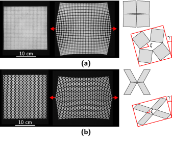
Figure 1: Response of planar kirigami to the heterogeneous loading conditions indicated by the arrows. (a) Rotating Squares pattern; (b) another pattern featuring rhombi slits. Insets depict representative unit cells in reference and deformed configurations, with actuation angles $\xi$ and $\gamma$.

Setup and overview of results – Kirigami traditionally describes an elastic sheet with a pattern of cuts and folds Callens and Zadpoor (2018); Sussman et al. (2015); Wang et al. (2017). More recently, the term has come to include cut patterns that, by themselves, produce complex deformations both in and out-of-plane Cho et al. (2014); Rafsanjani and Pasini (2016); Tang and Yin (2017); Blees et al. (2015); Rafsanjani and Bertoldi (2017); Dias et al. (2017); Konaković-Luković et al. (2018); Celli et al. (2018); Choi et al. (2019). Here, we study the 2D response of patterns with repeating unit cells of four convex quadrilateral panels and four parallelogram slits. These patterns form a large model system for mechanism-based kirigami Yang and You (2018); Singh and van Hecke (2021); Dang et al. (2022a); their pure mechanism deformations are unit-cell periodic and counter-rotate the panels. Fig. 1 shows two examples, with the familiar RS pattern in (a). Each kirigami is free to deform as a mechanism under the loading, yet curiously neither does. Instead, exotic soft modes reveal themselves in the response.

What determines soft modes? The key insight is that each unit cell is approximately mechanistic, yielding a bulk actuation that varies slowly from cell to cell. To characterize the response, then, one must solve the geometry problem of “fitting together” many nearly mechanistic cells. Coarse-graining this problem, we derive a continuum field theory coupling the kirigami’s macroscopic or effective deformation to the local motion of its unit cells. For each cell, we track the opening angle $2\xi$ of its deformed slit, along with an angle $\gamma$ giving the cell’s overall rotation as in Fig. 1. We derive a system of partial differential equations (PDEs) relating these angles, whose coefficients depend nonlinearly on $\xi$ as well as on the unit cell design. Solving this system exactly, we demonstrate an excellent match with experiments of different designs.

Our theory divides planar kirigami into two generic classes, which we term elliptic and hyperbolic based on the so-called type of the coarse-grained PDE Courant and Hilbert (2008); Evans (2010). Elliptic kirigami shows a characteristic decay in actuation away from loads. In contrast, hyperbolic kirigami deforms with persistent actuation, via a nonlinear wave response. Surprisingly, this dichotomy turns out to be directly related to the Poisson’s ratio of the unit cell—elliptic kirigami is auxetic, while hyperbolic kirigami is not. This result serves as a powerful demonstration of our continuum field theory, and adds to the emerging literature connecting Poisson’s ratio to the qualitative behavior of mechanical metamaterials Wei et al. (2013); Nassar et al. (2017); Lebée et al. (2018); Rocklin et al. (2017).

Coarse-graining planar kirigami – We begin by introducing a general kirigami pattern consisting of a periodic array of unit cells, each having four quad panels and four parallelogram slits as in Fig. 2(a). The most general setup is as follows: start by selecting a seed of two quad panels connected at a corner point, rotate a copy of this seed $180^{\mathrm{o}}$, and connect it to the original seed to form a unit cell. Provided the resulting panels are disjoint, tessellating this unit cell along a Bravais lattice with basis vectors $\mathbf{s}=\mathbf{s}_{1}+\mathbf{s}_{2}+\mathbf{s}_{3}+\mathbf{s}_{4}$ and $\mathbf{t}=\mathbf{t}_{1}+\mathbf{t}_{2}+\mathbf{t}_{3}+\mathbf{t}_{4}$ gives a viable pattern. For an explanation of why this procedure is exhaustive, see supplemental section SM.1 sup . We fix one such pattern and coarse-grain its kinematics.

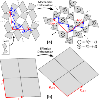
Figure 2: Coarse-graining a mechanism. (a) Vectors $\mathbf{s}_{i},\mathbf{t}_{i}$ define the unit cell, which tessellates along $\mathbf{s}$ and $\mathbf{t}$ to produce the pattern. In a mechanism, panels rotate by the indicated rotation matrices $\mathbf{R}(\gamma\pm\xi)$. (b) Coarse-graining through the lattice defines the effective deformation gradient $\mathbf{F}_{\text{eff}}$. Soft modes agree locally with this picture.

First, we consider mechanisms. As our kirigami has parallelogram slits, its pure mechanism deformations are given by an alternating array of panel rotations specified by the rotation matrices $\mathbf{R}(\gamma\pm\xi)$ in Fig. 2(a). (The angles $\gamma$ and $\xi$ agree with those of Fig. 1.) To coarse-grain, we view the deformation as distorting the underlying Bravais lattice: from the top half of the figure, the original lattice vectors $\mathbf{s}$ and $\mathbf{t}$ deform to

$$\mathbf{s}_{\text{def}}=\mathbf{R}(\gamma)\big{(}\mathbf{R}(-\xi)(\mathbf{s}_{1}+\mathbf{s}_{2})+\mathbf{R}(\xi)(\mathbf{s}_{3}+\mathbf{s}_{4})\big{)},$$ (1)

$$\mathbf{t}_{\text{def}}=\mathbf{R}(\gamma)\big{(}\mathbf{R}(-\xi)(\mathbf{t}_{1}+\mathbf{t}_{4})+\mathbf{R}(\xi)(\mathbf{t}_{2}+\mathbf{t}_{3})\big{)}.$$

In turn, this distortion can be encoded into the two-by-two matrix $\mathbf{F}_{\text{eff}}$ defined by $\mathbf{F}_{\text{eff}}\mathbf{s}=\mathbf{s}_{\text{def}}$ and $\mathbf{F}_{\text{eff}}\mathbf{t}=\mathbf{t}_{\text{def}}$, concretely linking Fig. 2(a) and (b). We call $\mathbf{F}_{\text{eff}}$ the coarse-grained or effective deformation gradient associated with the mechanism. Evidently,

$$\mathbf{F}_{\text{eff}}=\mathbf{R}(\gamma)\mathbf{A}(\xi)$$ (2)

for a shape tensor $\mathbf{A}(\xi)$ that depends only on $\xi$ and on the vectors $\mathbf{s}_{i}$ and $\mathbf{t}_{i}$ defining the unit cell. This tensor will be made explicit in the examples to come (see SM.2 sup for the general formula).

Having coarse-grained the pattern’s mechanisms, we now extend our viewpoint to its exotic soft modes of deformation, whose elastic energy scaling is less than bulk. Specifically, we consider elastic effects accounting for the finite size and distortion of the inter-panel hinges, and show in SM.3 sup that the energy per unit area of the kirigami vanishes with an increasing number of cells provided its effective deformation $\mathbf{y}_{\text{eff}}(\mathbf{x})$ obeys

$$\nabla\mathbf{y}_{\text{eff}}(\mathbf{x})=\mathbf{R}(\gamma(\mathbf{x}))\mathbf{A}(\xi(\mathbf{x})).$$ (3)

While this PDE is trivially solved by the pure mechanisms in (2), it admits many other exotic solutions whose effective deformation gradients $\nabla\mathbf{y}_{\text{eff}}(\mathbf{x})$ and angle fields $\gamma(\mathbf{x})$ and $\xi(\mathbf{x})$ vary across the sample. The PDE characterizes soft modes in a doubly asymptotic limit of finely patterned kirigami, in which the hinges are small relative to the panels and the number of panels is large.

As gradients are curl-free, it follows by taking the curl of (3) that (SM.4 sup )

$$\nabla\gamma(\mathbf{x})=\boldsymbol{\Gamma}(\xi(\mathbf{x}))\nabla\xi(\mathbf{x})$$ (4)

for $\boldsymbol{\Gamma}(\xi)=\frac{\mathbf{A}^{T}(\xi)\mathbf{A}^{\prime}(\xi)}{\det\mathbf{A}(\xi)}\mathbf{R}(\tfrac{\pi}{2})$. Eq. (4) is a PDE reflecting the geometric constraint that every closed loop in the kirigami must remain closed. This PDE can sometimes be solved analytically for the angle fields, as we do in the examples below, but in general we imagine it will be solved numerically. After finding $\gamma(\mathbf{x})$ and $\xi(\mathbf{x})$, $\mathbf{y}_{\text{eff}}(\mathbf{x})$ can be recovered from (3) uniquely up to a translation. Eqs. (3-4) furnish a complete effective description of the locally mechanistic kinematics of any planar kirigami with a unit cell of four quad panels and four parallelogram slits.

Linear analysis, PDE type and Poisson’s ratio – While the effective description (3-4) is nonlinear, we can start to learn its implications for kirigami soft modes by linearizing about a pure mechanism. We do so first for the class of rhombi-slit kirigami, whose shape tensors $\mathbf{A}(\xi)$ are diagonal. This simplification greatly clarifies the exposition without compromising the generality of our results; we treat general patterns at the end of this section.

Per Fig. 3, a rhombi-slit kirigami is defined by parameters $\lambda_{1},\ldots,\lambda_{4}$ that can take any value in $[0,1]$, and an aspect ratio $a_{r}>0$:

$$\mathbf{A}(\xi)=\mu_{1}(\xi)\mathbf{e}_{1}\otimes\mathbf{e}_{1}+\mu_{2}(\xi)\mathbf{e}_{2}\otimes\mathbf{e}_{2},$$ (5)

$$\mu_{1}(\xi)=\cos\xi-\alpha\sin\xi,\quad\mu_{2}(\xi)=\cos\xi+\beta\sin\xi,$$

$$\alpha=a_{r}(\lambda_{4}-\lambda_{2}),\quad\beta=a_{r}^{-1}(\lambda_{1}-\lambda_{3}).$$

Note $\alpha$ and $\beta$ encode the geometry of the unit cell, $\mu_{1}(\xi)$ and $\mu_{2}(\xi)$ give the stretch or contraction of its sides under a mechanism, and $\mathbf{e}_{1}$ and $\mathbf{e}_{2}$ are unit vectors along the initial slit axes, as in Fig. 3. Finally, $\boldsymbol{\Gamma}(\xi)$ in (4) satisfies

$$\boldsymbol{\Gamma}(\xi)=\Gamma_{12}(\xi)\mathbf{e}_{1}\otimes\mathbf{e}_{2}+\Gamma_{21}(\xi)\mathbf{e}_{2}\otimes\mathbf{e}_{1}$$ (6)

for $\Gamma_{12}(\xi)=-\mu_{1}^{\prime}(\xi)/\mu_{2}(\xi)$ and $\Gamma_{21}(\xi)=\mu_{2}^{\prime}(\xi)/\mu_{1}(\xi)$. Eqs. (LABEL:eq:rhombiSlits-6) follow from (LABEL:eq:defBravais-2) after choosing appropriate $\mathbf{s}_{i}$ and $\mathbf{t}_{i}$ (SM.2 sup ).

Proceeding perturbatively, we write $\xi(\mathbf{x})=\xi_{0}+\delta\xi(\mathbf{x})$ and $\gamma(\mathbf{x})=\delta\gamma(\mathbf{x})$ for small angles $\delta\xi(\mathbf{x})$ and $\delta\gamma(\mathbf{x})$, and let $\mathbf{y}_{\text{eff}}(\mathbf{x})=\mathbf{A}(\xi_{0})\mathbf{x}+\mathbf{u}(\mathbf{A}(\xi_{0})\mathbf{x})$ for a small displacement $\mathbf{u}(\mathbf{y})$ about a pure mechanism with constant slit opening angle $2\xi_{0}$. (Taking $\gamma_{0}=0$ eliminates a free global rotation.) Expanding (3) to linear order and computing the strain $\boldsymbol{\varepsilon}(\mathbf{y})=\tfrac{1}{2}(\nabla\mathbf{u}(\mathbf{y})+\nabla\mathbf{u}^{T}(\mathbf{y}))$ yields

$$\boldsymbol{\varepsilon}(\mathbf{A}(\xi_{0})\mathbf{x})=\delta\xi(\mathbf{x})\left(\begin{array}[]{cc}\varepsilon_{1}(\xi_{0})&0\\ 0&\varepsilon_{2}(\xi_{0})\end{array}\right)$$ (7)

with $\varepsilon_{i}(\xi_{0})=\mu_{i}^{\prime}(\xi_{0})/\mu_{i}(\xi_{0})$, $i=1,2$. Similarly, expanding (4) to linear order and taking its curl gives that

$$0=\big{(}\Gamma_{21}(\xi_{0})\partial_{1}^{2}-\Gamma_{12}(\xi_{0})\partial_{2}^{2}\big{)}\delta\xi(\mathbf{x}).$$ (8)

Both equations must hold for the perturbation to be consistent with the effective theory.

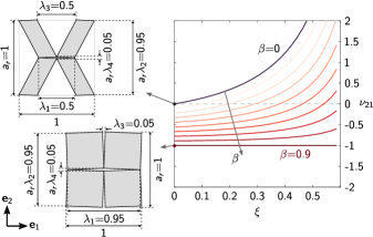
Figure 3: Effective Poisson’s ratio as a function of slit actuation $\xi$ for different rhombi-slit kirigami. The plot fixes $\alpha=-0.9$ and varies $\beta$ from $0$ to $0.9$. The RS pattern on the lower left sits at the lower extreme $\beta=0.9$. It is purely dilational ($\nu_{21}=-1$) and is auxetic for all $\xi$. The upper extreme $\beta=0$ arises with the design on the upper left, which is non-auxetic $(\nu_{21}>0)$ for all relevant $\xi>0$. Some designs transition between auxetic and non-auxetic behavior as a function of $\xi$.

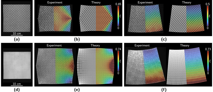
Figure 4: Comparison between theory and experiments of rhombi-slit kirigami. (a,d) Two $16\times 16$ cell patterns prior to deformation, with opposite Poisson’s ratios and types. Top row is non-auxetic and hyperbolic. Bottom row is auxetic and elliptic. (b,e) Left entries are experimental samples pulled along their centerlines. Right entries show simulations, based on exact solutions of the effective theory. (c,f) Annular deformations produced experimentally (left) and using the theory (right). Colormaps indicate the slit actuation angle $\xi(\mathbf{x})$, extracted from the experiment using the procedure in SM.7 sup .

The ratio of principal strains in (LABEL:eq:strain) defines an effective Poisson’s ratio which turns out to be directly related to the coefficients in (8):

$$\nu_{21}(\xi_{0}):=-\frac{\varepsilon_{2}(\xi_{0})}{\varepsilon_{1}(\xi_{0})}=\frac{\Gamma_{21}(\xi_{0})}{\Gamma_{12}(\xi_{0})}\frac{\mu_{1}^{2}(\xi_{0})}{\mu_{2}^{2}(\xi_{0})}.$$ (9)

This link has remarkable implications. Writing (8) as $\partial_{2}^{2}\delta\xi(\mathbf{x})=\tfrac{\mu_{2}^{2}(\xi_{0})}{\mu_{1}^{2}(\xi_{0})}\nu_{21}(\xi_{0})\partial_{1}^{2}\delta\xi(\mathbf{x})$ and applying standard PDE theory, we discover that the overall structure of the perturbations is governed by the sign of the Poisson’s ratio, i.e., by whether the pattern is auxetic or not:

$$\begin{cases}\nu_{21}(\xi_{0})<0\quad\text{ elliptic and auxetic},\\ \nu_{21}(\xi_{0})>0\quad\text{ hyperbolic and non-auxetic}.\end{cases}$$ (10)

This criterion is visualized in Fig. 3.

The terms hyperbolic and elliptic come from PDE theory where an equation’s type, found by linearization, informs the structure of its solutions Courant and Hilbert (2008); Evans (2010). Here in the hyperbolic case, (8) is the classical wave equation with wave speed $c=\tfrac{\mu_{2}(\xi_{0})}{\mu_{1}(\xi_{0})}\sqrt{\nu_{21}(\xi_{0})}$, the $x_{1}$- and $x_{2}$-coordinates being like “space” and “time”. Linearization predicts waves for small loads; motivated by this, we go on below to construct a branch of nonlinear wave solutions describing the hyperbolic kirigami in Fig. 1(b). In contrast, the RS pattern in Fig. 1(a) is auxetic and so is elliptic. Instead of waves, elliptic kirigami shows a decay in actuation away from loads. We highlight the strong maximum principle of elliptic PDEs Evans (2010): the maximum and minimum actuation in an elliptic kirigami must occur only at its boundary, lest it deform by a constant mechanism. No such principle holds for hyperbolic kirigami.

Remarkably, the same coupling in (10) between Poisson’s ratio and PDE type holds for the general quad-based kirigami patterns treated here. We sketch the main ideas to provide clarity on this important result (see SM.5 sup for details). Linearizing about a mechanism as before leads to a strain $\boldsymbol{\varepsilon}(\mathbf{A}(\xi_{0})\mathbf{x})$ with eigenvalues $\delta\xi(\mathbf{x})\varepsilon_{i}(\xi_{0})$, $i=1,2$. Passing to a principle frame, the effective Poisson’s ratio of the pattern—which dictates its auxeticity—is still given by the first expression in (9). Eq. (8) becomes a general second order linear PDE $c_{ij}(\xi_{0})\partial^{2}_{ij}\delta\xi(\mathbf{x})=0$ (summation implied). It is elliptic or hyperbolic according to the sign of the discriminant of its coefficients. A coordinate transformation reveals (10).

Nonlinear analysis and examples – The previous linear analysis addresses the character of the kirigami’s response nearby a pure mechanism, but does not prescribe it at finite loads. We now present several exact solutions of the nonlinear system (3-4) which capture the deformations of the kirigami in Fig. 4, far into the nonlinear response. Our solutions are based on known results from PDE theory, which we detail in SM.6 sup and summarize here. Using them, we simulate the panel motions with an ansatz that rotates and translates the panels to fit the solution. Due to the finiteness of the sample, one may expect slight deviations between theory and experiment, which scale with the relative panel size. See SM.3 sup for more details.

(i) Nonlinear waves – Fig. 4(a) shows the $\alpha=-0.9$, $\beta=0$ pattern from the top left of Fig. 3, which remains non-auxetic, thus hyperbolic, for $\xi\in(0,0.235\pi)$. The hyperbolicity is borne out through the existence of nonlinear simple wave solutions to (4), defined by the criteria that $\xi=\xi(\theta(\mathbf{x}))$ and $\gamma=\gamma(\theta(\mathbf{x}))$ for a scalar function $\theta(\mathbf{x})$. As a result, the angles vary across envelopes of straight line segments called characteristic curves. The term “simple wave” comes from compressible gas dynamics, where the same functional form governs gas densities varying next to regions of constant density Courant and Friedrichs (1999). For kirigami, simple waves alleviate slit openings next to regions of uniform actuation in response to loads.

The left part of Fig. 4(b) shows the experimental specimen pulled at its left and right ends along its centerline. Slits open by an essentially constant amount in a central diamond region (orange), and recede towards the specimen’s corners. Note the “fanning out” of contours of constant slit actuation from where the loads are applied. A simulation based on simple wave solutions matches these features on the right of Fig. 4(b). Its straight line contours are characteristic curves.

(ii) Conformal maps – Recent work Czajkowski et al. (2022) has noted the relevance of conformal maps for kirigami. Adding to this discussion, and as an example of our more general elliptic class, we note using (LABEL:eq:rhombiSlits) that the only rhombi-slit kirigami designs that deform conformally ($\mu_{1}(\xi)=\mu_{2}(\xi)$ for all $\xi$ by definition Do Carmo (2016)) have $\alpha=-\beta$ and $\nu_{21}(\xi)=-1$. This includes the RS pattern in Fig. 4(d), fabricated according to the lower left $\alpha=-0.9$ design in Fig. 3. We highlight the RS pattern due to its dramatic shape-morphing. Conformal mappings are basic examples in complex analysis Brown and Churchill (2009), enabling numerous solutions to (4).

The left part of Fig. 4(e) shows the RS pattern pulled at its left and right ends. Its slits open up dramatically at the loading points and remain closed at the corners: the largest and smallest openings are at the boundary, per the maximum principle. Contours of constant slit actuation form arcs around these points. On the right of Fig. 4(e), we fit the deformed boundary of the pattern to a conformal map. The simulation recovers the locations where the slits are most open and closed, and qualitatively matches their variations in the bulk.

(iii) Annuli – Though one may think of hyerperbolic and elliptic kirigami as a dichotomy, and this is true as far as auxeticity is concerned, we close by pointing out the existence of some special effective deformations that are “universal” in that they occur for both. One example is the annular deformation in Fig. 4(c) and (f), which arises from (4) under the condition that $\xi(\mathbf{x})$ is either only a function of $x_{1}$ or of $x_{2}$. All rhombi-slit kirigami patterns are capable of this deformation, as we demonstrate using the previous hyperbolic (c) and elliptic (f) designs. Note unlike the previous examples, these experiments are done using pure displacement boundary conditions.

Discussion – Looking forward, while our emphasis here was on the derivation of coarse-grained PDEs expressing bulk geometric constraints, we set aside the important question of the forces underlying them. Understanding the inter-panel forces more closely should eventually lead to a complete continuum theory predicting exactly which exotic soft mode will arise in response to a given load. Our results show that the effective PDE system (3-4) plays the dominant, constraining role. This is consistent with the conformal elasticity of Ref. Czajkowski et al. (2022).

More broadly, we expect that an effective PDE of a geometric origin exists to constrain the bulk behavior of mechanical metamaterials beyond kirigami. Such PDEs have been found for certain origami designs Nassar et al. (2017); Lebée et al. (2018), via a differential geometric argument akin to our passage from (3) to (4). In origami, one also finds a surprising coupling between the Poisson’s ratio of the mechanisms and certain fine features of exotic soft modes. Are such couplings universal? What about the role of heterogeneity Dudte et al. (2016); Celli et al. (2018); Choi et al. (2019); Dang et al. (2022b)? Can coarse-graining lead to constitutive models for mechanical metamaterials, common to practical engineering Khajehtourian and Kochmann (2021); McMahan et al. (2021), or to effective descriptions of their dynamics Deng et al. (2017)? While there are many avenues left to explore, our work on the soft modes of planar kirigami highlights new physics and is a convincing step towards the discovery of a continuum theory for mechanical metamaterials at large.

Acknowledgment. YZ and PP acknowledge support through PP’s start-up package at University of Southern California. IN and PC acknowledge the support of the Research Foundation for the State University of New York, and thank Megan Kam of iCreate for fabrication support. IT was supported by NSF award DMS-2025000.

References

- Mullin et al. (2007) T. Mullin, S. Deschanel, K. Bertoldi, and M. C. Boyce, Phys. Rev. Lett. 99, 084301 (2007).
- Bertoldi et al. (2017) K. Bertoldi, V. Vitelli, J. Christensen, and M. van Hecke, Nat. Rev. Mater. 2, 17066 (2017).
- Rafsanjani et al. (2019) A. Rafsanjani, K. Bertoldi, and A. R. Studart, Sci. Robot. 4, eaav7874 (2019).
- Kuribayashi et al. (2006) K. Kuribayashi, K. Tsuchiya, Z. You, D. Tomus, M. Umemoto, T. Ito, and M. Sasaki, Mater. Sci. Eng. A 419, 131 (2006).
- Velvaluri et al. (2021) P. Velvaluri, A. Soor, P. Plucinsky, R. L. de Miranda, R. D. James, and E. Quandt, Sci. Rep. 11, 1 (2021).
- Zirbel et al. (2013) S. A. Zirbel, R. J. Lang, M. W. Thomson, D. A. Sigel, P. E. Walkemeyer, B. P. Trease, S. P. Magleby, and L. L. Howell, J. Mech. Des. 135, 111005 (2013).
- Pellegrino and Calladine (1986) S. Pellegrino and C. R. Calladine, Int. J. Solids Struct. 22, 409 (1986).
- Hutchinson and Fleck (2006) R. G. Hutchinson and N. A. Fleck, J. Mech. Phys. Solids 54, 756 (2006).
- Milton (2013) G. W. Milton, J. Mech. Phys. Solids 61, 1543 (2013).
- Lubensky et al. (2015) T. C. Lubensky, C. L. Kane, X. Mao, A. Souslov, and K. Sun, Rep. Prog. Phys. 78, 073901 (2015).
- Coulais et al. (2018) C. Coulais, C. Kettenis, and M. van Hecke, Nat. Phys. 14, 40 (2018).
- Alibert et al. (2003) J.-J. Alibert, P. Seppecher, and F. Dell’Isola, Math. Mech. Solids 8, 51 (2003).
- Abdoul-Anziz and Seppecher (2018) H. Abdoul-Anziz and P. Seppecher, Math. Mech. Complex Syst. 6, 213 (2018).
- Schenk and Guest (2013) M. Schenk and S. D. Guest, Proc. Natl. Acad. Sci. U.S.A. 110, 3276 (2013).
- Wei et al. (2013) Z. Y. Wei, Z. V. Guo, L. Dudte, H. Y. Liang, and L. Mahadevan, Phys. Rev. Lett. 110, 215501 (2013).
- Grima and Evans (2000) J. N. Grima and K. E. Evans, J. Mater. Sci. Lett. 19, 1563 (2000).
- Deng et al. (2020) B. Deng, S. Yu, A. E. Forte, V. Tournat, and K. Bertoldi, Proc. Natl. Acad. Sci. U.S.A. 117, 31002 (2020).
- Czajkowski et al. (2022) M. Czajkowski, C. Coulais, M. van Hecke, and D. Z. Rocklin, Nat. Commun. 13, 211 (2022).
- Callens and Zadpoor (2018) S. J. P. Callens and A. A. Zadpoor, Mater. Today 21, 241 (2018).
- Sussman et al. (2015) D. M. Sussman, Y. Cho, T. Castle, X. Gong, E. Jung, S. Yang, and R. D. Kamien, Proc. Natl. Acad. Sci. U.S.A. 112, 7449 (2015).
- Wang et al. (2017) F. Wang, X. Guo, J. Xu, Y. Zhang, and C. Q. Chen, J. Appl. Mech. 84, 061007 (2017).
- Cho et al. (2014) Y. Cho, J.-H. Shin, A. Costa, T. A. Kim, V. Kunin, J. Li, S. Y. Lee, S. Yang, H. N. Han, I.-S. Choi, and D. J. Srolovitz, Proc. Natl. Acad. Sci. U.S.A. 111, 17390 (2014).
- Rafsanjani and Pasini (2016) A. Rafsanjani and D. Pasini, Extreme Mech. Lett. 9, 291 (2016).
- Tang and Yin (2017) Y. Tang and J. Yin, Extreme Mech. Lett. 12, 77 (2017).
- Blees et al. (2015) M. K. Blees, A. W. Barnard, P. A. Rose, S. P. Roberts, K. L. McGill, P. Y. Huang, A. R. Ruyack, J. W. Kevek, B. Kobrin, D. A. Muller, et al., Nature 524, 204 (2015).
- Rafsanjani and Bertoldi (2017) A. Rafsanjani and K. Bertoldi, Phys. Rev. Lett. 118, 084301 (2017).
- Dias et al. (2017) M. A. Dias, M. P. McCarron, D. Rayneau-Kirkhope, P. Z. Hanakata, D. K. Campbell, H. S. Park, and D. P. Holmes, Soft Matter 13, 9087 (2017).
- Konaković-Luković et al. (2018) M. Konaković-Luković, J. Panetta, K. Crane, and M. Pauly, ACM Trans. Graph. 37, 106 (2018).
- Celli et al. (2018) P. Celli, C. McMahan, B. Ramirez, A. Bauhofer, C. Naify, D. Hofmann, B. Audoly, and C. Daraio, Soft Matter 14, 9744 (2018).
- Choi et al. (2019) G. P. T. Choi, L. H. Dudte, and L. Mahadevan, Nat. Mater. 18, 999 (2019).
- Yang and You (2018) Y. Yang and Z. You, J. Mech. Robot. 10, 021001 (2018).
- Singh and van Hecke (2021) N. Singh and M. van Hecke, Phys. Rev. Lett. 126, 248002 (2021).
- Dang et al. (2022a) X. Dang, F. Feng, H. Duan, and J. Wang, Phys. Rev. Lett. 128, 035501 (2022a).
- Courant and Hilbert (2008) R. Courant and D. Hilbert, Methods of mathematical physics: partial differential equations (John Wiley & Sons, 2008).
- Evans (2010) L. C. Evans, Partial differential equations (American Mathematical Society, Providence, R.I., 2010).
- Nassar et al. (2017) H. Nassar, A. Lebée, and L. Monasse, Proc. Royal Soc. A 473, 20160705 (2017).
- Lebée et al. (2018) A. Lebée, L. Monasse, and H. Nassar, in 7th International Meeting on Origami in Science, Mathematics and Education (7OSME), Vol. 4 (Tarquin, 2018) p. 811.
- Rocklin et al. (2017) D. Z. Rocklin, S. Zhou, K. Sun, and X. Mao, Nat. Commun. 8, 1 (2017).
- (39) See Supplemental Material for further theoretical and experimental details.
- Courant and Friedrichs (1999) R. Courant and K. O. Friedrichs, Supersonic flow and shock waves, Vol. 21 (Springer Science & Business Media, 1999).
- Do Carmo (2016) M. P. Do Carmo, Differential geometry of curves and surfaces: revised and updated second edition (Courier Dover Publications, 2016).
- Brown and Churchill (2009) J. W. Brown and R. V. Churchill, Complex variables and applications eighth edition (McGraw-Hill Book Company, 2009).
- Dudte et al. (2016) L. H. Dudte, E. Vouga, T. Tachi, and L. Mahadevan, Nat. Mater. 15, 583 (2016).
- Dang et al. (2022b) X. Dang, F. Feng, P. Plucinsky, R. D. James, H. Duan, and J. Wang, International Journal of Solids and Structures 234, 111224 (2022b).
- Khajehtourian and Kochmann (2021) R. Khajehtourian and D. M. Kochmann, J. Mech. Phys. Solids 147, 104217 (2021).
- McMahan et al. (2021) C. McMahan, A. Akerson, P. Celli, B. Audoly, and C. Daraio, arXiv preprint arXiv:2107.01704 (2021).
- Deng et al. (2017) B. Deng, J. R. Raney, V. Tournat, and K. Bertoldi, Phys. Rev. Lett. 118, 204102 (2017).