Motion Planning for Variable Topology Trusses: Reconfiguration and Locomotion

Abstract

Truss robots are highly redundant parallel robotic systems that can be applied in a variety of scenarios. The variable topology truss (VTT) is a class of modular truss robots. As self-reconfigurable modular robots, a VTT is composed of many edge modules that can be rearranged into various structures depending on the task. These robots change their shape by not only controlling joint positions as with fixed morphology robots, but also reconfiguring the connectivity between truss members in order to change their topology. The motion planning problem for VTT robots is difficult due to their varying morphology, high dimensionality, the high likelihood for self-collision, and complex motion constraints. In this paper, a new motion planning framework to dramatically alter the structure of a VTT is presented. It can also be used to solve locomotion tasks that are much more efficient compared with previous work. Several test scenarios are used to show its effectiveness. Supplementary materials are available at https://www.modlabupenn.org/vtt-motion-planning/.

I Introduction

Modular self-reconfigurable robots consist of repeated building blocks (modules) with uniform docking interfaces that allow the transfer of forces and moments, power, and communication between modules [1]. These systems are capable of reconfiguring themselves to handle failures and adapt to changing environments. Many self-reconfigurable modular robots have been developed, with the majority being lattice or chain type systems [1]. In lattice modular robots ([2, 3]), modules are regularly positioned on a three-dimensional grid. Chain modular robots, such as [4, 5], consist of modules that form tree-like structures with kinematic chains that form articulated arms. Some systems are hybrid ([6, 7, 8]) and move like chain systems for articulated tasks but reconfigure using lattice-like actions.

Modular truss robots are made of beams that form parallel structures. The variable geometry truss (VGT) [9] is a modular robotic truss system with prismatic joints as truss members [10, 11, 12, 13]. These truss members change their lengths to alter the shape of the truss. The variable topology truss (VTT) is similar to the variable geometry truss robots with added ability to self-reconfigure the connection between members changing the truss topology [14, 15]. One current hardware prototype is shown in Fig. 1.

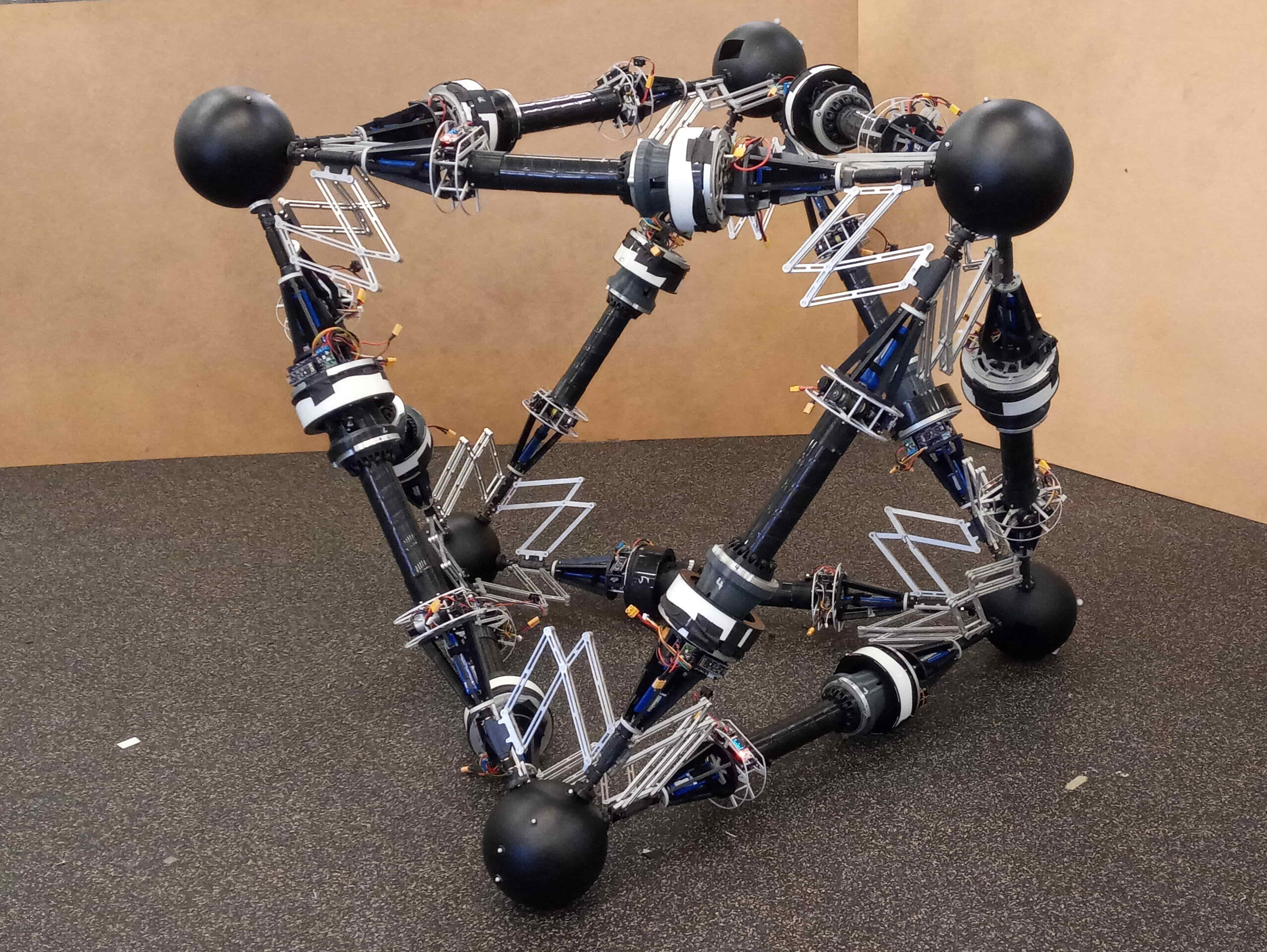
Figure 1: The hardware prototype of a VTT in octahedron configuration is composed of 12 members. Note that at least 18 members are required for topology reconfiguration [14].

A significant advantage for self-reconfigurable modular robots is their ability to adapt their morphologies to suit different requirements. For example, a VTT in which the members form a long chain could be used as a radio tower, or it could reconfigure to form a dome as a shelter in a disaster scenario. However, a fundamental complication with VTT systems comes from the motion of the complex parallel structure that has a high probability of self-collision. Developing self-collision-free motion plans is difficult due to the large number of degrees of freedom (DOFs) leading to very large search spaces.

A truss is composed of truss members (beams) and nodes (the connection points of multiple beams). A VTT is composed of edge modules each of which is one active prismatic joint member and passive joint ends that can actively attach or detach from other edge module ends [14]. The configuration can be fully defined by the set of member lengths and their node assignments at which point the edge modules are joined. A node is constructed by multiple edge module ends using a linkage system with a passive rotational DOF. The node assignments define the topology or how truss edge modules are connected, and the length of every member defines the shape of the resulting system [16]. Thus, there are two types of reconfiguration motions: geometry reconfiguration and topology reconfiguration. Geometry reconfiguration involves moving positions of nodes by changing lengths of corresponding members and topology reconfiguration involves changing the connectivity among members.

There are several physical constraints for a VTT to execute reconfiguration activities. A VTT has to be a rigid structure in order to maintain its shape and be statically determinant. A node in a VTT must be of degree three, so has to be attached by at least three members to ensure its controllability. In addition, A VTT requires at least 18 members before topology reconfiguration is possible [14]. Thus, motion planning for VTT systems has to deal with at least 18 dimensions and typically more than 21 dimensions. These constraints complicate the motion planning problem.

As VTTs are inherently parallel robots, it is easier to solve inverse kinematics than forward kinematics. So, for geometry reconfiguration, rather than planning for the active DOFs — the member lengths — we plan the motion of the nodes and then use inverse kinematics to determine the member lengths. However, the edge module arrangement in a VTT can result in a complicated configuration space even for a single node (nominally a 3-DOF problem) while keeping the others rigid.

Some desired paths for a node may be impossible to achieve without self-collision. Topology reconfiguration can often fix this. For example, some nodes may be split into two nodes to go around blocking members and then merge again on the other side. This process requires motion planning for two nodes at the same time. In addition, multiple nodes must move in coordination in order to achieve locomotion.

This paper builds on a sampling-based motion planning framework presented in our previous conference paper [17]. In this conference paper, we showed that the collision avoidance in geometry reconfiguration planning for simplified VTT models (nodes are considered as points and members are considered as line segments) can be handled efficiently by explicitly computing the configuration space for a group of nodes resulting in a smaller sampling space and a simpler collision model. We also extended the approach from [18] to compute all separated enclosed free spaces for a single node so that a sequence of topology reconfiguration actions can be computed by exploring these spaces using a simple rule. This paper adds significantly beyond the conference version in the following. We first solved the geometry reconfiguration planning with realistic physical hardware constraints being considered, including the sizes of the mechanical components, the actuator limitations, robot stability, and motion manipulability (to avoid singular configurations). For topology reconfiguration planning, the simple rule from our conference paper that is only based on the configuration space of simplified VTT models is limited when considering all physical constraints. A better sampling strategy is presented to handle this new difficulty so that enough samples can span the free space as much as possible and also provide topology reconfiguration actions as many as possible. These samples can then be used to search a sequence of actions for a given reconfiguration task. Finally, we present a novel locomotion framework based on this motion planning approach which controls a VTT to locomote without receiving external impact and achieves more robust and efficient performance compared with existing locomotion planning algorithms for truss robots.

The rest of the paper is organized as follows. Section II reviews relevant works and some necessary concepts are introduced in Section III as well as the problem statement. All the motion constraints are introduced in Section IV. Section V presents the geometry reconfiguration algorithm with motion of multiple nodes involved. Section VI introduces the approach to verify whether a topology reconfiguration action is needed and the planning algorithm to do topology reconfiguration. The locomotion planning approach is discussed in Section VII. Our framework is demonstrated in several test scenarios and compared with other approaches in Section VIII. Finally, Section IX talks about the conclusion and some future work.

II Related Work

In order to enable modular robots to adapt themselves to different activities and tasks, many reconfiguration planning algorithms have been developed over several decades for a variety of modular robotic systems [19, 20, 21, 8]. The planning framework includes topology reconfiguration where undocking (disconnecting two attached modules) and docking (connecting two modules) actions are involved. There are also some approaches for shape morphing and manipulation tasks, including inverse kinematics for highly redundant chains using PolyBot [22], constrained optimization techniques with nonlinear constraints [23], and a real-time quadratic programming approach with linear constraints [24]. In these works, there are no topology reconfiguration actions involved, but complicated kinematic structures and planning in high dimensional spaces need to be considered. However, these methods are not applicable to truss systems which have a very different morphology and connection architecture. Indeed the physical constraints and the collision models are significantly different from all of the previous lattice and chain type systems.

Some approaches have been developed for VGT systems that are similar to VTT systems, but do not include topology reconfiguration. Kinematic control is presented in [10] but is limited to tetrahedrons or octahedrons. Linear actuator robots (LARs) with a shape morphing algorithm are introduced in [12]. These systems are in mesh graph topology constructed by multiple convex hulls, and therefore self-collision can be avoided easily. However, this does not apply to VTT systems because edge modules span the workspace in a very non-uniform manner. There has been some work on VTT motion planning. The retraction-based RRT algorithm was developed in [15] in order to handle this high dimensional problem with narrow passage difficulty that is a well-known issue in sampling-based planning approaches; nevertheless, this approach is not efficient because it samples the whole workspace for every node and the collision checking needs to be done for every pair of members. Also, sometimes waypoints have to be assigned manually. A reconfiguration motion planning framework inspired by the DNA replication process — the topology of DNA can be changed by cutting and resealing strands as tanglements form — is presented in [16]. This work is based on a new method to discretize the workspace depending on the space density and an efficient way to check self-collision. Both topology reconfiguration actions and geometry reconfiguration actions are involved if needed. However, only a single node is involved in each step and the transition model is more complicated, which makes the algorithm limited in efficiency.

A fast algorithm to compute the configuration space of a given node in a VTT which is usually a non-convex space is presented in [18] and this space can be then decomposed into multiple convex polyhedrons so that a simple graph search algorithm can be applied to plan a path for this node efficiently. However, multiple nodes are usually involved in shape morphing tasks. In this paper, we first extend this approach to compute the obstacles for multiple nodes so that the search space can be decreased significantly. In addition, only the collision among a small number of edge modules needs to be considered when moving multiple nodes at the same time. Hence sampling-based planners can be applied efficiently. The idea has been discussed briefly in [25]. For some motion tasks, topology reconfiguration is required. An updated algorithm is developed to compute the whole not fully connected free space and required topology reconfiguration actions can then be generated using a hybrid planning framework (sampling-based and search-based) which can achieve behaviors that are similar to the DNA replication process.

The VTT locomotion process is similar to a locomotion mode of some VGTs which is accomplished by tipping and contacting the ground. TETROBOT systems and others have been shown with this mode in simulation with generated paths for moving nodes [26, 27]. These works divide the locomotion gait into several steps, but they have to compute the motion of nodes beforehand which cannot be applied to arbitrary configurations. Optimization approaches have been used for locomotion planning. The locomotion process can be formulated as a quadratic program by constraining the motion of the center of mass [12]. The objective function is related to the velocity of each node. A more complete quadratic programming approach to locomotion is presented in [28] to generate discrete motions of nodes in order to follow a given trajectory or compute a complete gait cycle. More hardware constraints were considered, including length and collision avoidance. However, the approach has to solve an optimization problem in high dimensional space, and it also has to deal with non-convex and nonlinear constraints which may cause numerical issues and is limited to a fully connected five-node graph in order to avoid incorporating the manipulability constraints into the quadratic program. This optimization-based approach is extended in [29] by preventing a robot from receiving impacts from the ground. Incorporated with a polygon-based random tree search algorithm to output a sequence of supporting polygons, a VTT can execute a locomotion task in an environment [30]. However, in these quadratic programs, numerical differentiation is required to relate some physical constraints with these optimized parameters whenever solving the problem. A locomotion step has to be divided into multiple phases leading to more constraints. Also, these approaches are not guaranteed to provide feasible solutions and they are also time-consuming to solve. In this paper, we present a new locomotion planning solution based on our efficient geometry reconfiguration planning algorithm. Our solution can solve the problem much faster and more reliably under several hardware constraints compared with previous works. This approach can be applied to arbitrary truss robots.

III Preliminaries and Problem Statement

A VTT can be represented as an undirected graph $G=(V,E)$ where $V$ is the set of vertices of $G$ and $E$ is the set of edges of $G$: each member can be regarded as an edge $e\in E$ of the graph and every intersection among members can be treated as a vertex $v\in V$ of the graph denoting a node. The Cartesian coordinates of a node $v\in V$ is $q^{v}=[v_{x},v_{y},v_{z}]^{\intercal}\in\mathbb{R}^{3}$ and the configuration space of node $v$ denoted as $\mathcal{C}^{v}$ is simply $\mathbb{R}^{3}$. In this way, the state of a member $e=(v_{1},v_{2})\in E$ where $v_{1}$ and $v_{2}$ are two vertices of edge $e$ can be fully defined by $q^{v_{1}}$ and $q^{v_{2}}$. The position of a given node $v\in V$ is controlled by changing the lengths of all attached members denoted as $E^{v}\subseteq E$.

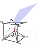
(a)

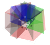
(b)

Figure 2: (a) Given node $v_{0}$, one of its neighbors $v_{1}$ and a member $(v_{6},v_{8})$ can define the blue polygon which is part of $\mathcal{C}_{\mathrm{obs}}^{v_{0}}$. (b) The obstacle region $\mathcal{C}_{\mathrm{obs}}^{v_{0}}$ is composed of polygons and the leftover space of $\mathbb{R}^{3}$ is $\mathcal{C}_{\mathrm{free}}^{v}$.

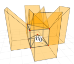
Figure 3: $\mathcal{C}_{\mathrm{free}}^{v_{0}}(q^{v_{0}})$ is bounded by polygons and workspace boundaries.

The geometry reconfiguration motion planning of a VTT is achieved by planning the motion of the involved nodes then determining the required member length trajectories. Given $v\in V$ in $G=(V,E)$, the state of every member $e\in E^{v}$, denoted as $\mathcal{A}^{v}(q^{v})$, can be altered by changing $q^{v}$. The obstacle region of this node that includes self-collision with other members as obstacles $\mathcal{C}^{v}_{\mathrm{obs}}\subseteq\mathcal{C}^{v}=\mathbb{R}^{3}$ is defined as

$$\mathcal{C}^{v}_{\mathrm{obs}}=\{q^{v}\in\mathbb{R}^{3}|\mathcal{A}^{v}(q^{v})\cap\mathcal{O}^{v}\neq\emptyset\}$$ (1)

where $\mathcal{O}^{v}$ is the obstacle for $E^{v}$. It is proved that this obstacle region is fully defined by the states of $\forall e\in E\setminus E^{v}$ and composed of multiple polygons [18]. For a simple VTT shown in Fig. 2a, the obstacle region $\mathcal{C}_{\mathrm{obs}}^{v_{0}}$ is shown in Fig. 2b. The free space of $v$ is just the leftover configurations denoted as

$$\mathcal{C}_{\mathrm{free}}^{v}=\mathbb{R}^{3}\setminus\mathcal{C}_{\mathrm{obs}}^{v}$$ (2)

However, $\mathcal{C}_{\mathrm{free}}^{v}$ may not be fully connected and is usually partitioned by $\mathcal{C}_{\mathrm{obs}}^{v}$. Only the enclosed subspace containing $q^{v}$ which is denoted as $\mathcal{C}_{\mathrm{free}}^{v}(q^{v})$ is free for node $v$ to move. A fast algorithm to compute the boundary of this subspace is presented in [18]. For example, given the VTT in Fig. 2a, $\mathcal{C}_{\mathrm{free}}^{v_{0}}$ — the free space of $v_{0}$ — is partitioned by $\mathcal{C}_{\mathrm{obs}}^{v_{0}}$ in Fig. 2b, and the subspace $\mathcal{C}_{\mathrm{free}}^{v_{0}}(q^{v_{0}})$ is shown in Fig. 3.

$\mathcal{C}_{\mathrm{free}}^{v}$ is usually partitioned by $\mathcal{C}_{\mathrm{obs}}^{v}$ into multiple enclosed subspaces, and it is impossible to move $v$ from one enclosed subspace to another one without topology reconfiguration. The physical system constraints shown in [14] allow two atomic actions on nodes that enable topology reconfiguration: Split and Merge. Since the physical system must be statically determinate with all nodes of degree three, a node $v$ must be composed of six or more edge modules to undock and split into two new nodes $v^{\prime}$ and $v^{\prime\prime}$, and both nodes should still have three or more members. This process is called Split. Two separate nodes are able to merge into an individual one in a Merge action. The simulation of these two actions is shown in Fig. 4. We are not considering splitting a node recursively, namely after splitting a node $v$ into $v^{\prime}$ and $v^{\prime\prime}$, further splitting $v^{\prime}$ or $v^{\prime\prime}$, because it is difficult to attach more than nine members to a single node due to physical hardware constraints. In a topology reconfiguration process, the number of nodes can change, but the number of members that are physical elements remains constant.

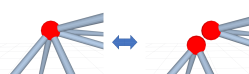
Figure 4: A single node with six members can be split into a pair of nodes and two separate nodes can also merge into an individual node.

In this work, given a VTT $G=(V,E)$, the reconfiguration planning problem can be stated as the following:

• Geometry Reconfiguration. For a set of $n$ nodes $\{v_{t}\in V|t=1,2,\cdots,n\}$, compute paths $\tau_{t}:\left[0,1\right]\to\mathcal{C}_{\mathrm{free}}^{v_{t}}$ such that $\tau_{t}(0)=q_{i}^{v_{t}}$ and $\tau_{t}(1)=q_{g}^{v_{t}}$ in which $t=1,2,\cdots,n$, $q_{i}^{v_{t}}$ is the initial position of $v_{t}$ and $q_{g}^{v_{t}}$ is the goal position of $v_{t}$.

• Topology Reconfiguration. Compute the topology reconfiguration actions, Merge and Split, and find collision-free path(s) to move a node $v$ from its initial position $q_{i}^{v}$ to its goal position $q_{g}^{v}$.

The shape of a VTT $G=(V,E)$ can be regarded as a polyhedron with flat polygonal facets formed by members. This polyhedron consists of vertices (a subset of $V$), edges $E^{G}$, facets $F^{G}$, and an incidence relation on them (e.g., every edge is incident to two vertices and every edge is incident to two facets [31]). One of the facets $f\in F^{G}$ is the current support polygon. In a rolling locomotion step, the support polygon is changed from $f$ to an adjacent facet $f^{\prime}$. The non-impact locomotion problem for a given VTT $G=(V,E)$ can be stated as the following:

• Non-impact Rolling Locomotion. Compute the motions of a set of nodes in $V$ such that a sequence of support polygons $f\in F^{G}$ can be generated in which adjacent facet $f^{\prime}\in F^{G}$ are used for each support polygon and the transition between two adjacent support polygons occur with all nodes from both facets are co-planar in contact with the ground.

IV Motion Constraints

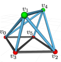
Figure 5: This VTT is composed of twelve members. Currently, the motion of node $v_{1}$ and node $v_{4}$ are under control by seven blue members.

Given a VTT $G=(V,E)$, the motions of nodes are controlled by all attached actuated members and the system is often an overconstrained parallel robot. We follow the modeling way in [10] to model a VTT and additionally provide a general kinematics model for truss robots. The set of all nodes $V$ is separated into two groups: $V_{F}$ and $V_{C}$ where $V_{F}$ contains all the fixed or stationary nodes and $V_{C}$ contains all the controlled nodes. For example, given the VTT shown in Fig. 5, when controlling the motion of node $v_{1}$ and node $v_{4}$, $V_{C}=\{v_{1},v_{4}\}$ and $V_{F}=\{v_{0},v_{2},v_{3},v_{5}\}$. This is a 6-DOF system since there are two controlled nodes. In addition, this system is overconstrained and the motion of two nodes are controlled by seven members. Note that $V_{F}$ and $V_{C}$ are not constant and they can be changed during the motion of a VTT (reconfiguration and locomotion). All motions of a VTT have to satisfy physical constraints in order to be feasible. In addition to these physical constraints, a VTT has to maintain infinitesimally rigidity or avoid singular configurations.

IV-A Hardware and Environmental Constraints

IV-A1 Length Constraints

In a VTT, each edge module has an active prismatic joint called Spiral Zipper [32] that is able to achieve a high extension ratio and form a high strength-to-weight-ratio column. The mechanical components determine the minimum member length and the total material determines the maximum member length. Hence, in a VTT $G=(V,E)$, $\forall e=(v_{i},v_{j})\in E$, we have the following constraint

$$\overline{L}_{\mathrm{min}}\leq\|q^{v_{i}}-q^{v_{j}}\|\leq\overline{L}_{\mathrm{max}}$$ (3)

IV-A2 Collision Avoidance

During the motion task, a VTT has to avoid self-collision. The distance between every two member axes must be greater than $\bar{d}_{\mathrm{min}}$, the diameter of an edge module which is a cylinder. The minimum distance between member $(v_{i},v_{j})$ and $(v_{m},v_{n})$ can be expressed as

$$\min\|(q^{v_{i}}+\alpha(q^{v_{j}}-q^{v_{i}}))-(q^{v_{m}}+\gamma(q^{v_{n}}-q^{v_{m}}))\|$$ (4)

in which $\alpha,\gamma\in(0,1)$. This is not easy to compute and can be more complicated when both members are moving. In Section V, we will show a way to avoid this problem. We also need to ensure that the angle between connected members remains larger than a minimum physical joint limit. The angle constraint between member $(v_{i},v_{j})$ and $(v_{i},v_{k})$ can be expressed as

$$\arccos\left(\frac{(q^{v_{j}}-q^{v_{i}})\bullet(q^{v_{k}}-q^{v_{i}})}{\|q^{v_{j}}-q^{v_{i}}\|\|q^{v_{k}}-q^{v_{i}}\|}\right)\geq\bar{\theta}_{\mathrm{min}}$$ (5)

IV-A3 Stability

The truss structure of a VTT is meant to be statically stable under gravity when interacting with the environment and sufficient constraints must be satisfied to ensure the location of the structure is fully defined. At least three still nodes should be on the ground in order to form a valid support polygon. For the VTT shown in Fig. 5, $v_{0}$, $v_{2}$, $v_{3}$, and $v_{5}$ are stationary on the ground to form the current support polygon. In addition, the vertical projection of the center of mass of a VTT on the ground has to be inside this support polygon. Furthermore, no collision is allowed between a VTT and the environment, and the simplest condition is that all nodes have to be above the ground.

IV-B Manipulability Maintenance Constraint

In order to control the motions of nodes, a VTT has to maintain the manipulability for these moving nodes to make sure the system is not close to singularity. For a VTT $G=(V,E)$, given $V_{C}$ with $\Lambda$ nodes under control, the position vector of this system is simply the stack of $q^{v}$ where $v\in V_{C}$. This system is controlled by all members that are attached with these nodes, namely $\bigcup_{v\in V_{C}}E^{v}$. Let $l_{ij}$ be the link vector from a controlled node $v_{i}$ pointing to any node $v_{j}$. There are two types of link vectors: 1. if $v_{j}\in V_{F}$, then $l_{ij}$ is an attachment link vector; 2. if $v_{j}\in V_{C}$, then $l_{ij}$ is a connection link vector. The link vector satisfies the following equation:

$$l_{ij}=q^{v_{j}}-q^{v_{i}}$$ (6)

in which $v_{i}\in V_{C}$. Taking the time derivative of both sides of Eq. (6) for an attachment link vector and a connection link vector to relate node velocities to joint velocities yields

$$l_{ij}^{\intercal}\dot{l}_{ij}=(q^{v_{i}}-q^{v_{j}})^{\intercal}\dot{q}^{v_{i}}\quad\forall v_{j}\in V_{F}$$ (7a)

$$\dot{l}_{ij}=\dot{q}^{v_{j}}-\dot{q}^{v_{i}}\quad\forall v_{j}\in V_{C}$$ (7b)

Assume $V_{C}=\{\bar{v}_{\alpha}|\alpha=1,2,\cdots,\Lambda\}$, and for a controlled node $\bar{v}_{\alpha}$, all the fixed nodes in its neighborhood $\mathcal{N}_{G}(\bar{v}_{\alpha})$ are denoted as $\hat{v}_{1}^{\alpha},\hat{v}_{2}^{\alpha},\cdots,\hat{v}_{N}^{\alpha}$, and the corresponding attachment link vectors are denoted as ${{}^{\alpha}}\hat{l}_{1},{{}^{\alpha}}\hat{l}_{2},\cdots,{{}^{\alpha}}\hat{l}_{N}$. Eq. (7a) is true for any ${{}^{\alpha}}\hat{l}_{t}$ where $t\in\left[1,N\right]$, so we can rewrite it for this controlled vertex $\bar{v}_{\alpha}$

$$B_{\alpha}\dot{L}_{\alpha}=A_{\alpha}\dot{q}^{\bar{v}_{\alpha}}$$ (8)

in which

$$\dot{L}_{\alpha}=\left[\begin{array}[]{cccc}{{}^{\alpha}}\dot{\hat{l}}_{1}^{\intercal}&{{}^{\alpha}}\dot{\hat{l}}_{2}^{\intercal}&\cdots&{{}^{\alpha}}\dot{\hat{l}}_{N}^{\intercal}\end{array}\right]^{\intercal}_{3N\times 1}$$

$$B_{\alpha}=\left[\begin{array}[]{cccc}{{}^{\alpha}}\hat{l}_{1}^{\intercal}&0&\cdots&0\\ 0&{{}^{\alpha}}\hat{l}_{2}^{\intercal}&\cdots&0\\ \vdots&\vdots&\ddots&\vdots\\ 0&0&\cdots&{{}^{\alpha}}\hat{l}_{N}^{\intercal}\end{array}\right]_{N\times 3N}$$

$$A_{\alpha}=\left[\begin{array}[]{cccc}q^{\bar{v}_{\alpha}}-q^{\hat{v}_{1}^{\alpha}}&q^{\bar{v}_{\alpha}}-q^{\hat{v}_{2}^{\alpha}}&\cdots&q^{\bar{v}_{\alpha}}-q^{\hat{v}_{N}^{\alpha}}\end{array}\right]^{\intercal}_{N\times 3}$$

If another controlled node $\bar{v}_{\beta}\in\mathcal{N}_{G}(\bar{v}_{\alpha})$, namely $\bar{v}_{\beta}$ is adjacent to $\bar{v}_{\alpha}$, then we have

$$\dot{\bar{l}}_{\alpha\beta}=\dot{q}^{\bar{v}_{\beta}}-\dot{q}^{\bar{v}_{\alpha}}$$ (9)

Combining Eq. (8) and Eq. (9), we get

$$\mathcal{B}\dot{\mathcal{L}}=\mathcal{A}\dot{p}$$ (10)

in which

$$p=\left[\begin{array}[]{cccc}(q^{\bar{v}_{1}})^{\intercal}&(q^{\bar{v}_{2}})^{\intercal}&\cdots&(q^{\bar{v}_{\Lambda}})^{\intercal}\end{array}\right]^{\intercal}$$

$$\dot{\mathcal{L}}=\left[\begin{array}[]{ccccccc}\dot{L}_{1}^{\intercal}&\dot{L}_{2}^{\intercal}&\cdots&\dot{L}_{\Lambda}^{\intercal}&\cdots&\dot{\bar{l}}_{\alpha\beta}&\cdots\end{array}\right]^{\intercal}$$

$$\mathcal{B}=\mathrm{diag}(B_{1},B_{2},\cdots,B_{\Lambda},\cdots,I,\cdots)\quad\mathcal{A}=\left[\mathcal{A}_{1},\mathcal{A}_{2}\right]^{\intercal}$$

$$\mathcal{A}_{1}=\mathrm{diag}(A_{1},A_{2},\cdots,A_{\alpha},\cdots,A_{\beta},\cdots,A_{\Lambda})$$

$$\mathcal{A}_{2}=\left[\begin{array}[]{ccccc}\vdots&\vdots&\vdots&\vdots&\vdots\\ 0_{3\times 3\alpha}&I_{3\times 3}&0_{3\times(\beta-\alpha-1)}&-I_{3\times 3}&0_{3\times 3(\Lambda-\beta)}\\ \vdots&\vdots&\vdots&\vdots&\vdots\end{array}\right]$$

The size of $\mathcal{A}_{2}$ is determined by the number of controlled vertices and connection link vectors (if there are $\omega$ connection link vectors, $\mathcal{A}_{2}$ is a $3\omega\times 3\Lambda$ matrix). For the system shown in Fig. 5, $\mathcal{A}_{2}=\left[I,-I\right]_{3\times 6}$ since there are only two controlled nodes and one connection link vector. It can be shown that $\mathcal{B}$ has full rank as long as there are no zero-length members whereas $\mathcal{A}$ may not have full rank. There must exist a set of link velocities, but some link velocities may result in invalid motions of nodes since the system can be overconstrained.

We can rearrange Eq. (10) in two ways:

$$\dot{\mathcal{L}}=\mathcal{B}^{+}\mathcal{A}\dot{p}=J_{\mathrm{BA}}\dot{p}$$ (11a)

$$\dot{p}=\mathcal{A}^{+}\mathcal{B}\dot{\mathcal{L}}=J_{\mathrm{AB}}\dot{\mathcal{L}}$$ (11b)

where $\mathcal{B}^{+}$ and $\mathcal{A}^{+}$ are the pseudo-inverse of $\mathcal{B}$ and $\mathcal{A}$ respectively, and both $J_{\mathrm{BA}}$ and $J_{\mathrm{AB}}$ matrices are the Jacobian. We use these two equations to describe the relationship between the link velocities and the controlled node velocities. $J_{BA}$ is always defined (as long as there is no zero-length member), but $J_{AB}$ may not be defined. Given $\dot{p}$ is known, Eq. (11a) gives the minimum norm solution to Eq. (10), namely minimizing $\|\dot{\mathcal{L}}\|$. On the other hand, Eq. (11b) results in the unique least square solution to Eq. (10) if $\dot{\mathcal{L}}$ is known, namely minimizing $\|\mathcal{B}\dot{\mathcal{L}}-\mathcal{A}\dot{p}\|$.

By applying singular value decomposition on $J_{\mathrm{AB}}$, its maximum singular value $\sigma_{\max}(J_{\mathrm{AB}})$ and minimum singular value $\sigma_{\min}(J_{\mathrm{AB}})$ can be derived, and the manipulability of the current moving nodes can be constrained as

$$\mu=\frac{\sigma_{\min}(J_{\mathrm{AB}})}{\sigma_{\max}(J_{\mathrm{AB}})}\geq\bar{\mu}_{\min}$$ (12)

V Geometry Reconfiguration

The overall shape of a VTT is altered by moving nodes around in the workspace. For an individual node, its configuration space is $\mathbb{R}^{3}$, and the configuration space for $n$ nodes is $\mathbb{R}^{3n}$. Our strategy to avoid this high dimensionality is to divide the moving nodes into multiple groups where each group contains one or a pair of nodes. The motion planning space for each group is either in $\mathbb{R}^{3}$ or $\mathbb{R}^{6}$ and we just need to solve a sequence of $\mathbb{R}^{3}$ or $\mathbb{R}^{6}$ path planning problems. Even with this lower-dimensional space, it is still a challenge to search for a valid solution. In addition, the resolution of a discretized space must be fine enough to ensure the motion of a member does not skip over a possible self-collision which leads to slow planning. We overcome these issues by computing the free space of the group in advance so that the sampling space is significantly decreased.

V-A Obstacle Region and Free Space

A group can contain either one node or a pair of nodes. Given a VTT $G=(V,E)$, for an individual node $v\in V$, an efficient algorithm to compute $\mathcal{C}_{\mathrm{obs}}^{v}$ and $\mathcal{C}_{\mathrm{free}}^{v}(q^{v})$ with its boundary is introduced in [18]. If there are two nodes $v_{i}\in V$ and $v_{j}\in V$ in a group, then any collision among members in $E^{v_{i}}$ and $E^{v_{j}}$ is treated as self-collision inside the group, and all the members in $E\setminus(E^{v_{i}}\cup E^{v_{j}})$ define the obstacle region of this group denoted as $\widehat{\mathcal{C}}_{\mathrm{obs}}^{v_{i}}$ (the obstacle region of $v_{i}$ in the group) and $\widehat{\mathcal{C}}_{\mathrm{obs}}^{v_{j}}$ (the obstacle region of $v_{j}$ in the group) respectively, namely

$$\widehat{\mathcal{C}}_{\mathrm{obs}}^{v_{i}}=\left\{q^{v_{i}}\in\mathbb{R}^{3}|\mathcal{A}^{v_{i}}(q^{v_{i}})\cap\mathcal{O}^{v_{i},v_{j}}\neq\emptyset\right\}$$

$$\widehat{\mathcal{C}}_{\mathrm{obs}}^{v_{j}}=\left\{q^{v_{j}}\in\mathbb{R}^{3}|\mathcal{A}^{v_{j}}(q^{v_{j}})\cap\mathcal{O}^{v_{i},v_{j}}\neq\emptyset\right\}$$

in which $\mathcal{O}^{v_{i},v_{j}}$ is formed by $\forall e\in E\setminus(E^{v_{i}}\cup E^{v_{j}})$.

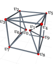
Figure 6: This VTT is composed of 21 edge modules with 10 nodes among which $v_{0}$ and $v_{1}$ form a group.

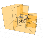
(a)

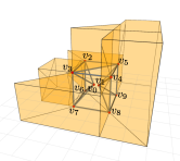
(b)

Figure 7: (a) $\widehat{\mathcal{C}}_{\mathrm{free}}^{v_{0}}(q^{v_{0}})$ is computed with all members controlling $v_{1}$ ignored. (b) $\widehat{\mathcal{C}}_{\mathrm{free}}^{v_{1}}(q^{v_{1}})$ is computed with all members controlling $v_{0}$ ignored.

Then the free space of this group can be derived as

$$\widehat{\mathcal{C}}_{\mathrm{free}}^{v_{i}}=\mathbb{R}^{3}\setminus\widehat{\mathcal{C}}_{\mathrm{obs}}^{v_{i}}$$ (13)

$$\widehat{\mathcal{C}}_{\mathrm{free}}^{v_{j}}=\mathbb{R}^{3}\setminus\widehat{\mathcal{C}}_{\mathrm{obs}}^{v_{j}}$$ (14)

Using the same boundary search approach in [18], the boundary of $\widehat{\mathcal{C}}_{\mathrm{free}}^{v_{i}}(q^{v_{i}})$ — the enclosed subspace containing the current position of node $v_{i}$ — can be obtained efficiently. Similarly, the boundary of $\widehat{\mathcal{C}}_{\mathrm{free}}^{v_{j}}(q^{v_{j}})$ can be obtained. For example, given the VTT shown in Fig. 6, if node $v_{0}$ and $v_{1}$ form a group, then $\widehat{\mathcal{C}}_{\mathrm{free}}^{v_{0}}(q^{v_{0}})$ and $\widehat{\mathcal{C}}_{\mathrm{free}}^{v_{1}}(q^{v_{1}})$ can be computed and shown in Fig. 7. $\mathcal{C}_{\mathrm{free}}^{v_{0}}(q^{v_{0}})$ contains some space on the right side of $v_{1}$ because $E^{v_{1}}$ is ignored. This space shows that it is possible to move $v_{0}$ to locations that are currently blocked by $v_{1}$ since $v_{1}$ can be moved away. It is guaranteed that as long as $v_{0}$ is moving inside $\widehat{\mathcal{C}}_{\mathrm{free}}^{v_{0}}(q^{v_{0}})$ (the space shown in Fig. 7a), there must be no collision between any member in $E^{v_{0}}$ and any member in $E\setminus(E^{v_{0}}\cup E^{v_{1}})$. Similarly, no collision between any member in $E^{v_{1}}$ and any member in $E\setminus(E^{v_{0}}\cup E^{v_{1}})$ can happen if $v_{1}$ is moving inside $\widehat{\mathcal{C}}_{\mathrm{free}}^{v_{1}}(q^{v_{1}})$ (the space shown in Fig. 7b). In this way, when planning the motion of node $v_{0}$ and $v_{1}$ using RRT, a sample will only be generated inside $\widehat{\mathcal{C}}_{\mathrm{free}}^{v_{0}}(q^{v_{0}})$ and $\widehat{\mathcal{C}}_{\mathrm{free}}^{v_{1}}(q^{v_{1}})$, and we only need to consider self-collision in the group, namely the collision can only happen among members in $E^{v_{0}}\cup E^{v_{1}}$. There is a special case when these two nodes in the group are connected by a member. Both ends of the member are moving which is not considered by our obstacle model. This is an extra case that we need to check when doing the planning.

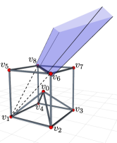
Figure 8: One obstacle polygon of $\mathcal{C}_{\mathrm{obs}}^{v_{0}}$ shown in Fig. 2a becomes a polyhedron bounded by five polygons if the sizes of VTT components are considered.

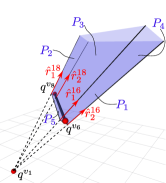
(a)

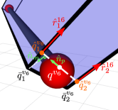
(b)

Figure 9: (a) Detailed illustration of the formation of the obstacle polyhedron. (b) Close view of the obstacle polyhedron.

The previous free space and the obstacle region are derived by ignoring the physical sizes of members and nodes (Fig. 2a). In practice, a node is a sphere and a member is a cylinder with non-zero radius. To make the system more realistic we can increase the derived obstacle region by considering the physical radii of VTT components. In the obstacle region, every polygon is converted into a polyhedron. For example, for the VTT shown in Fig. 2a, the purple polygon defined by node $v_{1}$ and edge module $(v_{6},v_{8})$ is one obstacle polygon for node $v_{0}$, and this polygon is converted into a polyhedron shown in Fig. 8. The boundary of this obstacle polyhedron is composed of five polygons that can be obtained as follows:

The current locations of nodes $v_{1}$, $v_{6}$, and $v_{8}$ are $q^{v_{1}}$, $q^{v_{6}}$, and $q^{v_{8}}$ respectively, and the unit vector normal to the plane formed by these three nodes is $\hat{n}_{p}$ ($-\hat{n}_{p}$ is also a normal unit vector but in the opposite direction). As shown in Fig. 9b, we first adjust $q^{v_{6}}$ and $q^{v_{8}}$ by moving them along $\hat{n}_{p}$ and $-\hat{n}_{p}$ respectively:

$$\hat{q}^{v_{6}}_{1}=q^{v_{6}}+\lambda\hat{n}_{p},\ \hat{q}^{v_{6}}_{2}=q^{v_{6}}-\lambda\hat{n}_{p}$$

$$\hat{q}^{v_{8}}_{1}=q^{v_{8}}+\lambda\hat{n}_{p},\ \hat{q}^{v_{8}}_{2}=q^{v_{8}}-\lambda\hat{n}_{p}$$

where $\lambda$ is the growing size that needs to consider the physical sizes of the mechanical components. $\lambda$ is usually set to be slightly larger than the sum of the radius of the node and the radius of the edge. Then, the four rays shown in Fig. 9a can be derived as

$$\hat{r}^{16}_{1}=\frac{\hat{q}^{v_{6}}_{1}-q^{v_{1}}}{\left\|\hat{q}^{v_{6}}_{1}-q^{v_{1}}\right\|},\ \hat{r}^{16}_{2}=\frac{\hat{q}^{v_{6}}_{2}-q^{v_{1}}}{\left\|\hat{q}^{v_{6}}_{2}-q^{v_{1}}\right\|}$$

$$\hat{r}^{18}_{1}=\frac{\hat{q}^{v_{8}}_{1}-q^{v_{1}}}{\left\|\hat{q}^{v_{8}}_{1}-q^{v_{1}}\right\|},\ \hat{r}^{18}_{2}=\frac{\hat{q}^{v_{8}}_{2}-q^{v_{1}}}{\left\|\hat{q}^{v_{8}}_{2}-q^{v_{1}}\right\|}$$

$\hat{n}_{m}$ is the unit vector perpendicular to the edge $\left(v_{6},\ v_{8}\right)$, pointing to $v_{1}$ and lying on the plane formed by $v_{1}$, $v_{6}$, and $v_{8}$. Then $\hat{q}^{v_{6}}_{1}$, $\hat{q}^{v_{6}}_{2}$, $\hat{q}^{v_{8}}_{1}$, and $\hat{q}^{v_{8}}_{2}$ are moved by $\lambda/2$ projected on $\hat{n}_{m}$ along $-\hat{r}^{16}_{1}$, $-\hat{r}^{16}_{2}$, $-\hat{r}^{18}_{1}$, and $-\hat{r}^{18}_{2}$, respectively:

$$\bar{q}^{v_{6}}_{1} =\hat{q}^{v_{6}}_{1}-\frac{\lambda}{2\left|\hat{n}_{m}\cdot\hat{r}^{16}_{1}\right|}\hat{r}^{16}_{1}$$

$$\bar{q}^{v_{6}}_{2} =\hat{q}^{v_{6}}_{2}-\frac{\lambda}{2\left|\hat{n}_{m}\cdot\hat{r}^{16}_{2}\right|}\hat{r}^{16}_{2}$$

$$\bar{q}^{v_{8}}_{1} =\hat{q}^{v_{8}}_{1}-\frac{\lambda}{2\left|\hat{n}_{m}\cdot\hat{r}^{18}_{1}\right|}\hat{r}^{18}_{1}$$

$$\bar{q}^{v_{8}}_{2} =\hat{q}^{v_{8}}_{2}-\frac{\lambda}{2\left|\hat{n}_{m}\cdot\hat{r}^{18}_{2}\right|}\hat{r}^{18}_{2}$$

Thus, we can encode the polyhedron boundary that is formed by the five polygons shown in Fig. 9a as:

$$P_{1} =\left\{V=\left(\bar{q}^{v_{6}}_{1},\ \bar{q}^{v_{6}}_{2}\right),\ R=\left(\hat{r}^{16}_{1},\ \hat{r}^{16}_{2}\right)\right\}$$

$$P_{2} =\left\{V=\left(\bar{q}^{v_{8}}_{1},\ \bar{q}^{v_{8}}_{2}\right),\ R=\left(\hat{r}^{18}_{1},\ \hat{r}^{18}_{2}\right)\right\}$$

$$P_{3} =\left\{V=\left(\bar{q}^{v_{6}}_{1},\ \bar{q}^{v_{8}}_{1}\right),\ R=\left(\hat{r}^{16}_{1},\ \hat{r}^{18}_{1}\right)\right\}$$

$$P_{4} =\left\{V=\left(\bar{q}^{v_{6}}_{2},\ \bar{q}^{v_{8}}_{2}\right),\ R=\left(\hat{r}^{16}_{2},\ \hat{r}^{18}_{2}\right)\right\}$$

$$P_{5} =\left\{V=\left(\bar{q}^{v_{6}}_{1},\ \bar{q}^{v_{6}}_{2},\ \bar{q}^{v_{8}}_{1},\ \bar{q}^{v_{8}}_{2}\right)\right\}$$

Note that $P_{5}$ consists of no rays.

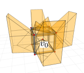
Figure 10: $\mathcal{C}_{\mathrm{free}}^{v_{0}}(q^{v_{0}})$ with physical sizes of components being considered.

Input: One obstacle polygon $P_{\mathrm{s}}$, the set of obstacle polygons $\mathcal{P}_{\mathrm{obs}}$

Output: A set of boundary polygons $\mathcal{P}_{\mathrm{b}}$

1 $\mathcal{P}_{\mathrm{b}}\leftarrow\emptyset$;

2 $\mathcal{Q}_{P}\leftarrow\emptyset$;

3 $\mathcal{Q}_{P}\text{.enqueue(}P_{\mathrm{s}}\text{)}$;

4 while $\mathcal{Q}_{P}\neq\emptyset$ do

5       $P_{i}\leftarrow\mathcal{Q}_{P}\text{.dequeue()}$;

6       $\mathcal{P}_{\mathrm{b}}\leftarrow\mathcal{P}_{\mathrm{b}}\cup\left\{P_{i}\right\}$;

7       foreach $s_{ij}\in S_{i}$ do

8             $\overline{P}_{ij}\leftarrow$ the innermost polygon in $\mathcal{N}_{ij}$;

9             if $\overline{P}_{ij}\notin\mathcal{P}_{\mathrm{b}}\wedge\overline{P}_{ij}\notin\mathcal{Q}_{P}$ then

10                   $\mathcal{Q}_{P}\text{.enqueue(}\overline{P}_{ij}\text{)}$;

11                  

12            

13      

return $\mathcal{P}_{\mathrm{b}}$

Algorithm 1 Boundary Search Algorithm

We can convert every obstacle polygon in Fig. 2b into an obstacle polyhedron (bounded by five polygons) and then process these polygons by Polygon Intersection and Boundary Search from [18] to derive $\mathcal{C}_{\mathrm{free}}^{v_{0}}(q^{v_{0}})$ shown in Fig. 10. The Boundary Search step can be simplified and the modified boundary search algorithm is shown in Algorithm 1. Recall that the free space of a node is usually partitioned by its obstacle region into multiple enclosed subspaces, and given an obstacle polygon $P_{\mathrm{s}}$ and the set of all obstacle polygons $\mathcal{P}_{\mathrm{obs}}$ generated by Polygon Intersection step [18], this algorithm can find the enclosed subspace with $P_{\mathrm{s}}$ being part of the boundary. Note that after Polygon Intersection, each polygon in $\mathcal{P}_{\mathrm{obs}}$ can only bound one enclosed subspace because every obstacle polygon is the boundary between the free space and the obstacle region. If we want to find the boundary of $\mathcal{C}_{\mathrm{free}}^{v_{0}}(q^{v_{0}})$, we can set $P_{\mathrm{s}}$ to be the obstacle polygon that is closest to $q^{v_{0}}$. In the algorithm, $S_{i}$ is the set of all edges of polygon $P_{i}$, $s_{ij}$ is the $j$th edge of $P_{i}$, and $\mathcal{N}_{ij}$ is the set of all polygons that share $s_{ij}$ with $P_{i}$. For each $P_{i}$, its normal vector pointing outwards the obstacle region is computed, and $\overline{P}_{ij}$ in Line 8 is the innermost polygon in $\mathcal{N}_{ij}$ along the normal vector of $P_{i}$.

The new $\mathcal{C}_{\mathrm{free}}^{v_{0}}(q^{v_{0}})$ is smaller and bounded by more polygons. For a single node, if it is on the same plane with all of its neighbor nodes, then it is in a singular configuration and we will lose controllability of that node. To avoid this, we also add this plane to the obstacle polygon set when running the boundary search algorithm. By taking these constraints into consideration, we can derive $\widehat{\mathcal{C}}_{\mathrm{free}}^{v_{0}}(q^{v_{0}})$ and $\widehat{\mathcal{C}}_{\mathrm{free}}^{v_{1}}(q^{v_{1}})$ for the group containing $v_{0}$ and $v_{1}$ in the VTT shown in Fig. 6 and the result is shown in Fig. 11. In the rest of the paper, we will use the simpler free space ignoring these physical constraints for visualization purposes.

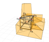
(a)

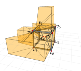
(b)

Figure 11: (a) $\widehat{\mathcal{C}}_{\mathrm{free}}^{v_{0}}(q^{v_{0}})$ is computed with all members controlling $v_{1}$ ignored. (b) $\widehat{\mathcal{C}}_{\mathrm{free}}^{v_{1}}(q^{v_{1}})$ is computed with all members controlling $v_{0}$ ignored.

V-B Path Planning for a Group of Nodes

If there is only one node $v$ in the group and the motion task is to move the node from its initial position $q_{i}^{v}$ to its goal position $q_{g}^{v}$ where $q_{i}^{v}\in\mathcal{C}_{\mathrm{free}}^{v}(q^{v}_{i})$ and $q_{g}^{v}\in\mathcal{C}_{\mathrm{free}}^{v}(q^{v}_{i})$ ($q_{i}^{v}$ and $q_{g}^{v}$ are in the same enclosed subspace), then it is straightforward to apply RRT approach in $\mathcal{C}_{\mathrm{free}}^{v}(q^{v}_{i})$ and no collision can happen as long as the motion of each step is inside $\mathcal{C}_{\mathrm{free}}^{v}(q^{v}_{i})$ since this space is usually not convex.

When moving two nodes $v_{i}$ and $v_{j}$ in a group, sampling will only happen inside $\widehat{\mathcal{C}}_{\mathrm{free}}^{v_{i}}(q^{v_{i}})$ and $\widehat{\mathcal{C}}_{\mathrm{free}}^{v_{j}}(q^{v_{j}})$ for $v_{i}$ and $v_{j}$ respectively. If there is no edge module connecting $v_{i}$ and $v_{j}$, then when applying RRT approach, the collision between moving members and fixed members can be ignored as long as the motion of both nodes in each step are inside $\widehat{\mathcal{C}}_{\mathrm{free}}^{v_{i}}(q^{v_{i}})$ and $\widehat{\mathcal{C}}_{\mathrm{free}}^{v_{j}}(q^{v_{j}})$ respectively. Only self-collision inside the group — the collision among members in $E^{v_{i}}\cup E^{v_{j}}$ — needs to be considered. If there is an edge module $e=(v_{i},v_{j})$ which connects $v_{i}$ and $v_{j}$, since this case is not included in our obstacle model when computing the obstacle region for the group, it is also necessary to check the collision between $e=(v_{i},v_{j})$ and every edge module in $E\setminus(E^{v_{i}}\cup E^{v_{j}})$.

In summary, when planning node $v_{i}$ and $v_{j}$ in a VTT $G=(V,E)$, for each step, in order to avoid collision, it is required to ensure the following:

• The motion of both node $v_{i}$ and $v_{j}$ are inside $\widehat{\mathcal{C}}_{\mathrm{free}}^{v_{i}}(q^{v_{i}})$ and $\widehat{\mathcal{C}}_{\mathrm{free}}^{v_{j}}(q^{v_{j}})$ respectively;

• No collision happens among edge modules in $E^{v_{i}}\cup E^{v_{j}}$;

• No collision happens between edge module $e=(v_{i},v_{j})$ and every edge module in $E\setminus(E^{v_{i}}\cup E^{v_{j}})$ if $e=(v_{i},v_{j})$ exists.

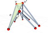
(a)

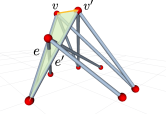
(b)

Figure 12: Light green triangle ($\blacktriangle$) is sweeped by member $e$ when moving node $v$ to new location $v^{\prime}$ along the yellow ($\bm{\rightarrow}$) trajectory and the new position of member $e$ is $e^{\prime}$. $e$ doesn’t collide with any other members in (a) but does collide with two members in (b) during the motion [16].

It is difficult to check the second and third collision case during the motion if both nodes are moving simultaneously. But since the step size for each node is limited and both of them are moving in straight lines, we can first check the collision during the motion of $v_{i}$ while keeping $v_{j}$ fixed, and then check the motion of $v_{j}$ [16]. Every edge module can be modeled as a line segment in space, thus, when moving node $v$, every $e\in E^{v}$ sweeps a triangle area, and if this member collides with another member $\bar{e}\in E$, then $\bar{e}$ must intersect with the triangle generated by $e$ (Fig. 12). Just as in Section V-A, we can buffer this triangle area to consider the component radii. Another way is to compute the local obstacle region of $v_{i}$ by only taking $E^{v_{j}}$ into account when moving $v_{i}$, and similarly compute the local obstacle region of $v_{j}$ by only taking $E^{v_{i}}$ into account when moving $v_{j}$. For $v_{i}$, given $\mathcal{N}_{G}(v_{i})$ that is the neighbors of $v_{i}$ and $E^{v_{j}}$, the local obstacle region of $v_{i}$ is the union of the obstacle polyhedrons $\forall(v,e)\in\mathcal{N}_{G}(v_{i})\times E^{v_{j}}$. Collisions occur if the line segment trajectory of $v_{i}$ intersects with its local obstacle region. Similarly for $v_{j}$. If edge module $(v_{i},v_{j})$ exists, when moving $v_{i}$, we also consider the obstacle polyhedron defined by $v_{j}$ and $e\in E\setminus(E^{v_{i}}\cup E^{v_{j}})$, and similarly the obstacle polyhedron defined by $v_{i}$ and $e\in E\setminus(E^{v_{i}}\cup E^{v_{j}})$ when moving $v_{j}$. In this way, we avoid solving Eq. (4).

In addition to this constraint we have the length constraint (Eq. 3), the angle constraint (Eq. 5), the manipulability constraint (Eq. 12), and the stability constraint when interacting with the environment. For these constraints, it is straightforward to check discretized states for validity. When checking the static stability constraint, we first find all supporting nodes by checking a nodes distance from the ground. The projected center of mass onto the ground must be within the convex hull formed by the supporting nodes on the ground.

We can efficiently check the state validity and motion validity, and RRT-type approaches can be applied. Open Motion Planning Library (OMPL) [33] is used to implement RRT for this path planning problem.

V-C Geometry Reconfiguration Planning

Assuming there are $n$ nodes $\{v_{t}\in V|t=1,2\cdots,n\}$ that should be moved from their initial positions $q_{i}^{v_{1}},q_{i}^{v_{2}},\cdots,q_{i}^{v_{n}}$ to their goal positions $q_{g}^{v_{1}},q_{g}^{v_{2}},\cdots,q_{g}^{v_{n}}$ respectively, we first divide these nodes into $\lceil n/2\rceil$ groups. Each group contains at most two nodes. The motion task is achieved by moving nodes one group at a time. Then this geometry reconfiguration problem results in a search for a sequence of group motions that can achieve the task. This approach solves the geometry reconfiguration planning problem faster than that in [18].

VI Topology Reconfiguration

Topology reconfiguration involves changing the connectivity among edge modules by docking and undocking. This reconfiguration process is often difficult for modular robotic systems so the necessary requirement for topology reconfiguration should be verified. Recall that the free space of a node is usually not a single connected component and if a motion task spans multiple connected components, if a solution exists it must include topology reconfiguration.

VI-A Enclosed Subspace in Free Space

As mentioned before, each polygon after Polygon Intersection in $\mathcal{C}_{\mathrm{obs}}^{v}$ bounds only one enclosed subspace. Therefore we can compute all the enclosed subspaces by repeatedly applying Algorithm 1 as shown in Algorithm 2.

In this algorithm, we first obtain the set of all obstacle polygons $\mathcal{P}_{\mathrm{obs}}^{v}$ by Polygon Intersection. Then, search for the enclosed subspace containing the current node configuration — $\mathcal{C}_{\mathrm{free}}^{v}(q^{v})$ — from a starting polygon $P_{\mathrm{s}}$ that is the nearest one to the node [18]. Afterward, we compute all other enclosed subspaces in $\mathcal{C}_{\mathrm{free}}^{v}$ by searching the boundary starting from any polygon that has not been used. Fig. 13 shows two enclosed subspaces of node $v_{0}$ in a simple cubic truss. In total, there are 33 enclosed subspaces in $\mathcal{C}_{\mathrm{free}}^{v_{0}}$ above the ground.

Input: VTT $G=(V,E)$, node $v\in V$

Output: The set of all enclosed subspaces $\mathcal{C}_{\mathrm{free}}^{v}$

1 Compute $\mathcal{P}_{\mathrm{obs}}$;

2 $P_{\mathrm{s}}\leftarrow$polygon closest to node $v$;

3 $\mathcal{C}_{\mathrm{free}}^{v}(q^{v})\leftarrow\textnormal{{BoundarySearch(}}\textnormal{\emph{$P_{\mathrm{s}},\ \mathcal{P}_{\mathrm{obs}}$}}\textnormal{{)}}$;

4 $\mathcal{C}_{\mathrm{free}}^{v}\leftarrow\left\{\mathcal{C}_{\mathrm{free}}^{v}(q^{v})\right\}$;

5 foreach $P_{i}\in\mathcal{P}_{\mathrm{obs}}^{v}$ do

6       if $P_{i}\notin\mathcal{C}\ \forall\mathcal{C}\in\mathcal{C}_{\mathrm{free}}^{v}$ then

7             $\mathcal{C}_{\mathrm{new}}\leftarrow\textnormal{{BoundarySearch(}}\textnormal{\emph{$P_{i},\ \mathcal{P}_{\mathrm{obs}}$}}\textnormal{{)}}$;

8             $\mathcal{C}_{\mathrm{free}}^{v}\leftarrow\mathcal{C}_{\mathrm{free}}^{v}\cup\{\mathcal{C}_{\mathrm{new}}\}$;

9            

10      

Algorithm 2 Enclosed Subspace Search

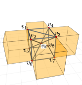
(a)

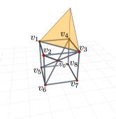
(b)

Figure 13: (a) Enclosed subspace $\mathcal{C}_{\mathrm{free}}^{v_{0}}(q^{v_{0}})$ contains the current position of $v_{0}$. (b) Another enclosed subspace is separated from $\mathcal{C}_{\mathrm{free}}^{v_{0}}(q^{v_{0}})$ by obstacles.

VI-B Topology Reconfiguration Actions

There are two topology reconfiguration actions for VTT: Split and Merge [14]. A node constructed by six or more edge modules can be split into two separate nodes (every node must have at least three edges). Two separate nodes can merge into one node. These actions can significantly affect the motions of the involved nodes with a variety of constraints. For the VTT shown in Fig. 6, $\mathcal{C}_{\mathrm{free}}^{v_{0}}(q^{v_{0}})$ that is the enclosed subspace containing the current location of node $v_{0}$ is shown in Fig. 14a. This node can move to some locations outside the truss but its motion is also blocked in some directions. The members attached with node $v_{1}$ blocked the motion of node $v_{0}$ on this side, and the plane formed by node $v_{2}$, $v_{3}$, $v_{6}$, and $v_{7}$ also blocks the motion of $v_{0}$ due to: 1. collision avoidance with member $(v_{2},v_{3})$, $(v_{2},v_{6})$, $(v_{3},v_{7})$, and $(v_{6},v_{7})$; 2. singularity avoidance that $v_{0}$ cannot move through the square formed by $v_{2}$, $v_{3}$, $v_{6}$, and $v_{7}$. If merging $v_{1}$ and $v_{0}$ as $v_{0}$ shown in Fig. 14b, $\mathcal{C}_{\mathrm{free}}^{v_{0}}(q^{v_{0}})$ will be changed. The boundary originally blocked by members attached with node $v_{1}$ disappears because all members controlling $v_{0}$ and $v_{1}$ are combined into a single set. In addition, this Merge action increases the motion manipulability of node $v_{0}$ so it can move through the square formed by $v_{2}$, $v_{3}$, $v_{6}$, and $v_{7}$. However, the reachable space is reduced such as the space above the truss and around the member $(v_{4},v_{8})$.

(a)

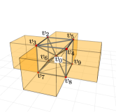
(b)

Figure 14: (a) Enclosed subspace $\mathcal{C}_{\mathrm{free}}^{v_{0}}(q^{v_{0}})$ when $v_{0}$ and $v_{1}$ are separated; (b) Enclosed subspace $\mathcal{C}_{\mathrm{free}}^{v_{0}}(q^{v_{0}})$ after merging $v_{1}$ with $v_{0}$.

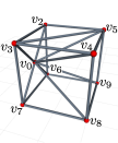
(a)

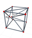
(b)

Figure 15: (a) Node $v_{0}$, $v_{2}$, $v_{3}$, $v_{6}$, and $v_{7}$ are on the same plane. (b) Splitting node $v_{0}$ in this way to separate $E^{v_{0}}$ into two sets is not valid, because node $v_{0}$ will be in singular configuration. Similarly, it is not valid to merge $v_{1}$ with $v_{0}$.

When executing a Split action on a node, one requirement is that this node must have at least six edge modules. Here we physically split one node into two and move them apart. In order to guarantee motion controllability, singularities should be avoided. For example, when node $v_{0}$ is on the same plane with node $v_{2}$, $v_{3}$, $v_{6}$, and $v_{7}$ shown in Fig. 15a, we cannot split node $v_{0}$ as in Fig. 15b, because one of the newly generated nodes ($v_{0}$ in this case) will be in a singular configuration. In comparison, if $v_{0}$ is outside the truss shown in Fig. 16a, then it is feasible to apply the same Split action to generate two new nodes shown in Fig. 16b. This constraint also applies for the Merge action. In Fig. 15b, since node $v_{0}$ is in a singular configuration, we cannot merge $v_{1}$ with $v_{0}$ to become a new truss shown in Fig. 15a. However, it is feasible to merge $v_{0}$ and $v_{1}$ in Fig. 16b to become $v_{0}$ in Fig. 16a.

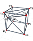
(a)

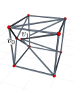
(b)

Figure 16: (a) Node $v_{0}$ is outside the truss. (b) It is possible to split node $v_{0}$ in this way to generate $v_{1}$. Reversely, $v_{0}$ and $v_{1}$ can be merged.

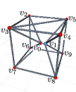
(a)

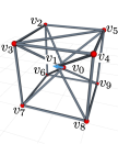
(b)

Figure 17: Split node $v_{0}$ into $v_{0}$ and $v_{1}$: (a) a right way to move node $v_{1}$ away from node $v_{0}$; (b) a wrong way to move node $v_{1}$ away from node $v_{0}$.

After splitting a node, the members attached to this node are separated into two groups that can be controlled independently. However, we need to consider how to move the two newly generate nodes away from each other. In Fig. 17a, after splitting $v_{0}$ into $v_{0}$ and $v_{1}$, $v_{1}$ is moved towards the right side of $v_{0}$ and this motion can separate the members without collision. However, in Fig. 17b, for the same Split action, $v_{1}$ is moved to the left side of $v_{0}$ which is not feasible because members will collide. When merging two nodes, we first need to move them to some locations that are close to each other. If the new locations are not selected correctly, it may be impossible to merge them.

VI-C Topology Reconfiguration Planning

Given a VTT $G=(V,E)$ and a motion task that is to move node $v$ from $q_{i}^{v}$ to $q_{g}^{v}$, if $q_{i}^{v}$ and $q_{g}^{v}$ belong to the same enclosed subspace, then geometry reconfiguration planning is able to handle this problem by either the approach in [18] or the approach introduced in Section V-B. Otherwise, topology reconfiguration is needed. The node has to execute a sequence of Split and Merge to avoid collision with other members.

There are multiple ways for a node $v$ to split into nodes $v^{\prime}$ and $v^{\prime\prime}$ as there are multiple ways to take the members into two groups. It is straightforward to compute all possible ways to split $E^{v}$ into two groups in which both sets contain at least three edge modules. Let $\mathcal{A}$ be the set of all possible ways to separate $E^{v}$ into two groups. If $v$ is split into $v^{\prime}$ and $v^{\prime\prime}$, then $E^{v}$ is separated into $E^{v^{\prime}}$ and $E^{v^{\prime\prime}}$ accordingly. This split process is denoted as $(E^{v^{\prime}},E^{v^{\prime\prime}})$. Not all possible ways in $\mathcal{A}$ can be applied on node $v$. Given a valid VTT $G=(V,E)$ and a node $v$, a Split action can be encoded as a tuple $(E^{v^{\prime}},E^{v^{\prime\prime}},q_{\mathrm{s}}^{v^{\prime}},q_{\mathrm{s}}^{v^{\prime\prime}})$ where $v^{\prime}$ and $v^{\prime\prime}$ are the newly generated node after splitting, and $q_{\mathrm{s}}^{v^{\prime}}$ and $q_{\mathrm{s}}^{v^{\prime\prime}}$ are the locations of these two new nodes. For simplicity, $q_{\mathrm{s}}^{v^{\prime}}=q^{v}$ and $v^{\prime\prime}$ is moved away from $v^{\prime}$ Function VI-C is used to search $q_{\mathrm{s}}^{v^{\prime\prime}}$ and compute a valid Split action.

[t!]    ComputeSplitAction($G$, $q^{v}$, $a\in\mathcal{A}$) Data: $D$, $\Delta D$, $D_{\max}$ Move node $v$ to $q^{v}$;

2 if VTTValidation($G$) = False then

3       return Null;

4      

5Split node $v$ into $v^{\prime}$ and $v^{\prime\prime}$ according to $a\in\mathcal{A}$;

6 $q_{\mathrm{s}}^{v^{\prime}}\leftarrow q^{v}$, $q_{\mathrm{s}}^{v^{\prime\prime}}\leftarrow q^{v}$;

7 Compute $d_{v}$;

8 repeat

9       $q_{\mathrm{s}}^{v^{\prime\prime}}=q^{v}+Dd_{v}$;

10       Move node $v^{\prime\prime}$ to $q^{v^{\prime\prime}}$;

11       if VTTCollisionCheck ($G$) = True then

12             $D\leftarrow(D+\Delta D)d_{v}$;

13            

14      else

15             if VTTValidation($G$) = True then

16                   return $(E^{v^{\prime}},E^{v^{\prime\prime}},q_{\mathrm{s}}^{v^{\prime}},q_{\mathrm{s}}^{v^{\prime\prime}})$;

17                  

18            else

19                   return Null;

20                  

21            

22      

23until $D>D_{\max}$;

24return Null;

 

In Function VI-C, $G$ is the given VTT, $a\in\mathcal{A}$ is one possible split, and $D$, $\Delta D$, and $D_{\max}$ are three parameters. The function VTTValidation checks the length constraints (Eq. (3)), the angle constraints (Eq. (5)), the stability constraint (Sec. IV-A3), and the manipulability constraint (Eq. (12)), and returns true if a given VTT satisfies all these hardware constraints, otherwise returns false. The function VTTCollisionCheck returns false if there is no collision among all members, otherwise it returns true. The basic idea is to move $v^{\prime\prime}$ gradually away from $v^{\prime}$ along a unit vector $d_{v}$ until a valid VTT is found. The direction of $d_{v}$ is determined by $q_{\mathrm{s}}^{v^{\prime}}$ (the current location of $v^{\prime}$) and $\mathcal{N}_{G}(v^{\prime})$ (the neighbors of $v^{\prime}$), and can be derived by normalizing the following vector:

$$\sum_{\hat{v}\in\mathcal{N}_{G}(v^{\prime})}\frac{q_{\mathrm{s}}^{v^{\prime}}-q^{\hat{v}}}{\|q_{\mathrm{s}}^{v^{\prime}}-q^{\hat{v}}\|}$$ (15)

and the distance moved along vector $d_{v}$ can be tried iteratively. The maximum distance between $v^{\prime}$ and $v^{\prime\prime}$ for searching is $D_{\max}$ that should be a small value. Within this small range, self-collision is a more significant constraint, such as in Fig. 17b. Hence collision checking occurs first then the other hardware constraints are checked. Conversely, if merging $v^{\prime}$ and $v^{\prime\prime}$ as $v$ at a location $q^{v}$, with this computed Split action $(E^{v^{\prime}},E^{v^{\prime\prime}},q_{\mathrm{s}}^{v^{\prime}},q_{\mathrm{s}}^{v^{\prime\prime}})$, first check if $q_{\mathrm{s}}^{v^{\prime}}=q^{v}\in\mathcal{C}_{\mathrm{free}}^{v^{\prime}}(q^{v^{\prime}})$ and $q_{\mathrm{s}}^{v^{\prime\prime}}\in\mathcal{C}_{\mathrm{free}}^{v^{\prime\prime}}(q^{v^{\prime\prime}})$, and if true, move $v^{\prime}$ to $q_{\mathrm{s}}^{v^{\prime}}$ and move $v^{\prime\prime}$ to $q_{\mathrm{s}}^{v^{\prime\prime}}$, and then merge them at $q^{v}$.

Given $q^{v}$, the current position of node $v$, and $\mathcal{C}_{\mathrm{free}}^{v}=\{{{}^{t}}\mathcal{C}_{\mathrm{free}}^{v}|t=1,2,\cdots,T\}$ that contains $T$ enclosed subspaces in the free space of node $v$, apply a valid Split action on this node to separate $E^{v}$ into $E^{v^{\prime}}$ and $E^{v^{\prime\prime}}$ and generate two new nodes $v^{\prime}$ and $v^{\prime\prime}$. $q^{v^{\prime}}$ and $q^{v^{\prime\prime}}$ are the locations of $v^{\prime}$ and $v^{\prime\prime}$, and $\mathcal{C}_{\mathrm{free}}^{v^{\prime}}(q^{v^{\prime}})$ and $\mathcal{C}_{\mathrm{free}}^{v^{\prime\prime}}(q^{v^{\prime\prime}})$ can be computed accordingly. Assuming there is a position $q\in{{}^{t}}\mathcal{C}_{\mathrm{free}}^{v}$ where node $v$ can also be split in the same way ($E^{v}$ can be separated into $E^{v^{\prime}}$ and $E^{v^{\prime\prime}}$ with Split action $(E^{v^{\prime}},E^{v^{\prime\prime}},q_{\mathrm{s}}^{v^{\prime}},q_{\mathrm{s}}^{v^{\prime\prime}})$), if $q_{\mathrm{s}}^{v^{\prime}}\in\mathcal{C}_{\mathrm{free}}^{v^{\prime}}(q^{v^{\prime}})$ and $q_{\mathrm{s}}^{v^{\prime\prime}}\in\mathcal{C}_{\mathrm{free}}^{v^{\prime\prime}}(q^{v^{\prime\prime}})$, namely $v^{\prime}$ and $v^{\prime\prime}$ can navigate to $q_{\mathrm{s}}^{v^{\prime}}$ and $q_{\mathrm{s}}^{v^{\prime\prime}}$ respectively and merge at $q$, then this node $v$ can navigate from $\mathcal{C}_{\mathrm{free}}^{v}(q^{v})$ to ${{}^{t}}\mathcal{C}_{\mathrm{free}}^{v}$ by a pair of Split and Merge actions, and these two enclosed subspaces can be connected under this action pair. This is the transition model when applying topology reconfiguration actions.

From Section VI-B, it is shown that the possible ways to split a node are highly dependent on the location of the node, and the resulting enclosed subspaces of the newly generated nodes can be different when splitting the node at different locations, so multiple samples are needed for every enclosed subspace. When applying the transition model described above, it is necessary to compute $\mathcal{C}_{\mathrm{free}}^{v^{\prime}}(q^{v^{\prime}})$ and $\mathcal{C}_{\mathrm{free}}^{v^{\prime\prime}}(q^{v^{\prime\prime}})$ many times (for every sample and every valid split action) and can be time-consuming. An alternative is to regard $v^{\prime}$ and $v^{\prime\prime}$ as a group and compute their group free space $\widehat{\mathcal{C}}_{\mathrm{free}}^{v^{\prime}}(q^{v^{\prime}})$ and $\widehat{\mathcal{C}}_{\mathrm{free}}^{v^{\prime\prime}}(q^{v^{\prime\prime}})$ respectively for every possible way to split $v$ in advance. For $v^{\prime}$, we can apply Algorithm 2 to search all enclosed subspaces ignoring all edge modules in $E^{v^{\prime\prime}}$ that is $\{{{}^{t}}\widehat{\mathcal{C}}_{\mathrm{free}}^{v^{\prime}}|t=1,2,\cdots,T^{\prime}\}$. Similarly, we can also derive $\{{{}^{t}}\widehat{\mathcal{C}}_{\mathrm{free}}^{v^{\prime\prime}}|t=1,2,\cdots,T^{\prime\prime}\}$ for $v^{\prime\prime}$ ignoring all edge modules in $E^{v^{\prime}}$. These two sets are independent of the location of node $v$. If $q_{\mathrm{s}}^{v^{\prime}}\in\widehat{\mathcal{C}}_{\mathrm{free}}^{v^{\prime}}(q^{v^{\prime}})$ and $q_{\mathrm{s}}^{v^{\prime\prime}}\in\widehat{\mathcal{C}}_{\mathrm{free}}^{v^{\prime\prime}}(q^{v^{\prime\prime}})$, then these two enclosed subspaces can be connected. This transition model based on the group free space can be much more efficient but may cause failures when applying the path planning for a group of nodes since it is less strict than the previous one.

Input: ${{}^{t}}\mathcal{C}_{\mathrm{free}}^{v}$, $G$, $\mathcal{A}$

Output: $\mathcal{S}$, $\mathcal{A}^{\mathcal{S}}$

1 $\mathcal{S}\leftarrow\emptyset$;

2 Initialize an empty map $\mathcal{A}^{\mathcal{S}}$;

3 Initialize $d_{\min}$;

4 $N_{\max}\leftarrow\textnormal{{SampleNumber(}}\textnormal{\emph{${{}^{t}}\mathcal{C}_{\mathrm{free}}^{v}$}}\textnormal{{)}}$;

5 for $k=1$ to $K$ do

6       $\mathcal{A}_{\mathrm{valid}}\leftarrow\emptyset$;;

7       $q_{\mathrm{rand}}\leftarrow\textnormal{{RandomPosition(}}\textnormal{\emph{${{}^{t}}\mathcal{C}_{\mathrm{free}}^{v}$}}\textnormal{{)}}$;

8       foreach $a\in\mathcal{A}$ do

9             $\hat{a}=\textnormal{{ComputeSplitAction(}}\textnormal{\emph{$G$, $q$, $a$}}\textnormal{{)}}$;

10             if $\hat{a}$ is not Null then

11                   $\mathcal{A}_{\mathrm{valid}}=\mathcal{A}_{\mathrm{valid}}\cup\{\hat{a}\}$;

12                  

13            

14      $\mathcal{S}_{\mathrm{close}}\leftarrow\left\{q|q\in\mathcal{S}\wedge\|q-q_{\mathrm{rand}}\|\leq d_{\min}\right\}$;

15       if $\mathcal{S}_{\mathrm{close}}=\emptyset\wedge|\mathcal{S}|<N_{\max}$ then

16             $\mathcal{S}\leftarrow\mathcal{S}\cup\{q_{\mathrm{rand}}\}$;

17             $\mathcal{A}^{\mathcal{S}}\left[q\right]=\mathcal{A}_{\mathrm{valid}}$;

18            

19       else if $\mathcal{S}_{\mathrm{close}}\neq\emptyset\wedge|\mathcal{S}|<N_{\max}$ then

20             if $|\mathcal{A}_{\mathrm{valid}}|=|\mathcal{A}|$ then

21                   foreach $q\in\mathcal{S}_{\mathrm{close}}$ do

22                         del $\mathcal{A}^{\mathcal{S}}\left[q\right]$;

23                        

24                  $\mathcal{S}\leftarrow\mathcal{S}\setminus\mathcal{S}_{\mathrm{close}}+\{q_{\mathrm{rand}}\}$;

25                   $\mathcal{A}^{\mathcal{S}}\left[q_{\mathrm{rand}}\right]=\mathcal{A}_{\mathrm{valid}}$;

26                  

27            else

28                   $\textnormal{{UpdateFlag}}\leftarrow\textsc{False}$;

29                   foreach $q\in\mathcal{S}_{\mathrm{close}}$ do

30                         if $\mathcal{A}^{\mathcal{S}}\left[q\right]\subset\mathcal{A}_{\mathrm{valid}}$ then

31                               del $\mathcal{A}^{\mathcal{S}}\left[q\right]$;

32                               $\mathcal{S}\leftarrow\mathcal{S}\setminus\{q\}$;

33                               $N_{\max}\leftarrow N_{\max}-1$;

34                               $\textnormal{{UpdateFlag}}\leftarrow\textsc{True}$;

35                              

36                         else if $\mathcal{A}_{\mathrm{valid}}\setminus\mathcal{A}^{\mathcal{S}}\left[q\right]\neq\emptyset$ then

37                               $\textnormal{{UpdateFlag}}\leftarrow\textsc{True}$;

38                              

39                        

40                  if $\textnormal{{UpdateFlag}}=\textsc{True}$ then

41                         $\mathcal{S}\leftarrow\mathcal{S}+\{q\}$;

42                         $\mathcal{A}^{\mathcal{S}}\left[q_{\mathrm{rand}}\right]=\mathcal{A}_{\mathrm{valid}}$;

43                         $N_{\max}\leftarrow N_{\max}+1$;

44                        

45                  

46            

47      

Algorithm 3 Sample Generation

There are two phases in the topology reconfiguration planning: sample generation and graph search. In sample generation, samples are generated providing as many valid Split actions as possible spanning the enclosed subspaces. We introduce Algorithm 3 to sample a given enclosed subspace. $\mathcal{S}$ is the set containing all generated samples and $\mathcal{A}^{\mathcal{S}}$ stores the Split actions for every sample. $N_{\max}$ is the maximum number of samples for a given enclosed subspace ${{}^{t}}\mathcal{C}^{v}_{\mathrm{free}}$ determined by the size of the space. In our setup, we find the range of a given space along $x$-axis, $y$-axis, and $z$-axis denoted as $x_{\mathrm{range}}$, $y_{\mathrm{range}}$, and $z_{\mathrm{range}}$ respectively, then $N_{\max}$ is $\left\lceil\sqrt{x_{\mathrm{range}}^{2}+y_{\mathrm{range}}^{2}+z_{\mathrm{range}}^{2}}\Big{/}d_{\min}\right\rceil$ in which $d_{\min}$ is the minimum distance between every pair of samples. $K$ is the maximum number of iterations set by users and can be related to $N_{\max}$. For each iteration, we first randomly generate a sample $q_{\mathrm{rand}}$ that is inside the given enclosed subspace, then find all valid Split actions stored in $\mathcal{A}_{\mathrm{valid}}$ (Line 6 — 11). Then find all previous valid samples that are close to $q_{\mathrm{rand}}$ (Line 12). If $q_{\mathrm{rand}}$ is far from all previous valid samples and the size of $\mathcal{S}$ is less than $N_{\max}$, add this new sample and store its valid Split actions (Line 13—15). If $q_{\mathrm{rand}}$ is close to some previous valid samples, there are two cases for consideration. If this new sample provides all possible Split actions, then remove all valid nearby samples and only keep this new sample for this area since this is the best option (Line 17—21). Otherwise, we check two conditions: 1. whether there exists any valid nearby sample that has fewer valid Split actions than $q_{\mathrm{rand}}$; 2. whether the new sample $q_{\mathrm{rand}}$ introduces any new Split actions compared with all valid nearby samples. If the first condition is true, remove the old sample and add the new sample to $\mathcal{S}$. If the second condition is true, add the new sample to $\mathcal{S}$ (Line: 23—35). We run Algorithm 3 for every enclosed subspace to generate enough samples, and then add $q_{i}^{v}$ (the initial location of node $v$) to the sample set of $\mathcal{C}^{v}_{\mathrm{free}}(q_{i}^{v})$ and add $q_{g}^{v}$ (the goal location of node $v$) to the sample set of $\mathcal{C}^{v}_{\mathrm{free}}(q_{g}^{v})$. After the sample generation phase, ${}^{\mathcal{C}}\mathcal{S}$ and the corresponding Split actions for all samples ${}^{\mathcal{C}}\mathcal{A}^{\mathcal{S}}$ are obtained $\forall\mathcal{C}\in\mathcal{C}_{\mathrm{free}}^{v}$.

The graph search phase follows. It generates a sequence of topology reconfiguration actions using the transition model discussed earlier. A graph search algorithm can be applied to compute a sequence of enclosed subspaces starting from $\mathcal{C}_{\mathrm{free}}^{v}(q_{i}^{v})$ to $\mathcal{C}_{\mathrm{free}}^{v}(q_{g}^{v})$ while exploring the topology connections among these enclosed subspaces. Fig. 18 is an example where the graph has enclosed subspaces as vertices. An edge in this graph connecting two enclosed subspaces denotes that node $v$ can move from a sample in one enclosed subspace to a sample in the other. The graph is built from $\mathcal{C}_{\mathrm{free}}^{v}(q^{v})$, grows as valid transitions among enclosed subspaces are found, and stops when the enclosed subspace containing $q_{g}^{v}$ is visited. A graph search algorithm based on Dijkstra’s framework is shown in Algorithm 4.

Figure 18: Topology connections among three enclosed subspaces of node $v$.

Line 1 — 4: If $q_{i}^{v}$ and $q_{g}^{v}$ are in the same enclosed subspace, then no topology reconfiguration is needed. Otherwise, we make two sets $\mathcal{Q}$ and $\overline{\mathcal{Q}}$ where $\mathcal{Q}$ contains all newly checked or non-visited enclosed subspaces and $\overline{\mathcal{Q}}$ contains all visited enclosed subspaces. The sizes of these two sets will change as the algorithm explores $\mathcal{C}_{\mathrm{free}}^{v}$. Initially, only the enclosed subspace containing $q_{i}^{v}$ that is $\mathcal{C}_{\mathrm{free}}^{v}(q_{i}^{v})$ and the enclosed subspace containing $q_{g}^{v}$ that is $\mathcal{C}_{\mathrm{free}}^{v}(q_{g}^{v})$ are in $\mathcal{Q}$, and the algorithm starts with $\mathcal{C}_{\mathrm{free}}^{v}(q_{i}^{v})$. The value $g(\mathcal{C})$ is the cost of the path from $q_{i}^{v}$ to the enclosed subspace $\mathcal{C}$, so $g(\mathcal{C}_{\mathrm{free}}^{v}(q_{i}^{v}))=0$ and $g(\mathcal{C}_{\mathrm{free}}^{v}(q_{g}^{v}))=\infty$ at the beginning.

Input: $G$, $q_{i}^{v}$, $q_{g}^{v}$, $\mathcal{C}_{\mathrm{free}}^{v}$, $\{({{}^{\mathcal{C}}}\mathcal{S},{{}^{\mathcal{C}}}\mathcal{A}^{\mathcal{S}})|\mathcal{C}\in\mathcal{C}_{\mathrm{free}}^{v}\}$

Output: Tree of enclosed subspaces $p$

1 if $\mathcal{C}_{\mathrm{free}}^{v}(q_{i}^{v})=\mathcal{C}_{\mathrm{free}}^{v}(q_{g}^{v})$ then

2       return Null;

3      

4$\mathcal{Q}\leftarrow\left\{\mathcal{C}_{\mathrm{free}}^{v}(q_{i}^{v}),\mathcal{C}_{\mathrm{free}}^{v}(q_{g}^{v})\right\}$, $\overline{\mathcal{Q}}\leftarrow\emptyset$;

5 $g(\mathcal{C}_{\mathrm{free}}^{v}(q_{i}^{v}))\leftarrow 0$, $g(\mathcal{C}_{\mathrm{free}}^{v}(q_{g}^{v}))\leftarrow\infty$;

6 while $\mathcal{C}_{\mathrm{free}}^{v}(q_{g}^{v})\in\mathcal{Q}$ do

7       $\overline{\mathcal{C}}\leftarrow\underset{\mathcal{C}\in\mathcal{Q}}{\arg\min}\ g(\mathcal{C})$;

8       $\mathcal{Q}\leftarrow\mathcal{Q}\setminus\{\overline{\mathcal{C}}\}$;

9       $\overline{\mathcal{Q}}\leftarrow\overline{\mathcal{Q}}\cup\{\overline{\mathcal{C}}\}$;

10       foreach $\mathcal{C}\in\mathcal{C}_{\mathrm{free}}^{v}\setminus\{\overline{\mathcal{C}}\}\wedge\mathcal{C}\notin\overline{\mathcal{Q}}$ do

11             foreach $({{}^{\overline{\mathcal{C}}}}q,{{}^{\mathcal{C}}}q)\in{{}^{\overline{\mathcal{C}}}}\mathcal{S}\times{{}^{\mathcal{C}}}\mathcal{S}$ do

12                   if ValidMotion(${}^{\overline{\mathcal{C}}}q$, ${}^{\mathcal{C}}q$) = True then

13                         if $\mathcal{C}\in\mathcal{Q}$ then

14                               if $g(\overline{\mathcal{C}})+c({{}^{\overline{\mathcal{C}}}}q,{{}^{\mathcal{C}}}q)<g(\mathcal{C})$ then

15                                     $g(\mathcal{C})\leftarrow g(\overline{\mathcal{C}})+c({{}^{\overline{\mathcal{C}}}}q,{{}^{\mathcal{C}}}q)$;

16                                     $p(\mathcal{C})\leftarrow\overline{\mathcal{C}}$;

17                                    

18                              

19                        else

20                               $\mathcal{Q}\leftarrow\mathcal{Q}+\{\mathcal{C}\}$;

21                               $g(\mathcal{C})\leftarrow g(\overline{\mathcal{C}})+c({{}^{\overline{\mathcal{C}}}}q,{{}^{\mathcal{C}}}q)$;

22                               $p(\mathcal{C})\leftarrow\overline{\mathcal{C}}$;

23                              

24                        break ;

25                        

26                  

27            

28      

Algorithm 4 Topology Reconfiguration Planning

Line 6 — 8: Every iteration starts with the enclosed subspace that has the lowest cost $g(\mathcal{C})$ in $\mathcal{Q}$. At the beginning, $\mathcal{C}_{\mathrm{free}}^{v}(q_{i}^{v})$ has the lowest cost. After selecting an enclosed subspace, update $\mathcal{Q}$ and $\overline{\mathcal{Q}}$.

Line 9 — 20: Iterate every enclosed subspace $\mathcal{C}$ except $\overline{\mathcal{C}}$ in $\mathcal{C}_{\mathrm{free}}^{v}$ and check if it is already visited. If so, then this potential transition is not a new transition. Otherwise, check if there exists a valid motion to move the node from any sample in $\overline{\mathcal{C}}$ that is the enclosed subspace with the lowest cost to any sample in $\mathcal{C}$ handled by Function ValidMotion. Both transition models are implemented and compared in the test scenarios. If this is true, then there are two cases: this subspace is not checked for the first time namely that there is already a connection between this enclosed subspace and another enclosed subspace, or this subspace has never been checked which means it has no connection before. For the first case, we need to check whether its cost needs to be updated. $c({{}^{\overline{\mathcal{C}}}}q,{{}^{\mathcal{C}}}q)$ is the cost of the motion from ${{}^{\overline{\mathcal{C}}}}q$ to ${{}^{\mathcal{C}}}q$. This cost can be related to the estimated distance or other factors. In our setup, all valid motions from one enclosed subspace to another one have the same cost. If its cost is updated, then its parent $p(\mathcal{C})$ should also be updated accordingly. For the second case, initialize the cost and the parent of this newly checked enclosed subspace, and update set $\mathcal{Q}$. There can be multiple ways to transit between two enclosed subspaces. For example, there are two edges between ${}^{t_{2}}\mathcal{C}_{\mathrm{free}}^{v}$ and ${}^{t_{3}}\mathcal{C}_{\mathrm{free}}^{v}$ shown in Fig. 18. In our setup, we just keep the first one being found. Since ${{}^{\overline{{\mathcal{C}}}}}\mathcal{S}$ and ${}^{\mathcal{C}}\mathcal{S}$ are randomly generated, it is possible that the condition in Line 11 is failed although there does exist ${}^{\overline{\mathcal{C}}}q$ and ${}^{\mathcal{C}}q$ that can pass this condition.

Once $\mathcal{C}_{\mathrm{free}}^{v}(q_{g}^{v})$ is visited, the algorithm ends. With $p$, a tree with visited enclosed subspaces as vertices, it is straightforward to find the optimal path connecting $\mathcal{C}_{\mathrm{free}}^{v}(q_{i}^{v})$ and $\mathcal{C}_{\mathrm{free}}^{v}(q_{g}^{v})$ as well as all the samples that the node needs to traverse. For example, in Fig. 18, when node $v$ traverses from ${}^{t_{1}}q_{1}^{v}$ to ${}^{t_{3}}q_{1}^{v}$, it first moves to ${}^{t_{1}}q_{2}^{v}$, then Split and Merge at ${}^{t_{3}}q_{2}^{v}$, and finally move to ${}^{t_{3}}q_{1}^{v}$. Moving a node inside one of its enclosed subspaces can be solved easily by geometry reconfiguration planning. After splitting the node, we can apply geometry reconfiguration planning to move them to the computed positions in the next enclosed subspace for merging.

VII Locomotion

Unlike the previous reconfiguration planning, the center of mass during locomotion moves over a large range. In a rolling locomotion step, a VTT rolls from one support polygon to an adjacent support polygon (Fig. 19a). In this process, it is useful to maintain statically stable locomotion to prevent the system from receiving impacts from the ground as repeated impacts may damage the reconfiguration nodes. Due to this requirement, previous implementations of a rolling locomotion step has manually divided into several phases [30, 28]. Our approach can deal with this issue automatically. A high-level path planner generates a sequence of support polygons for a given environment and the locomotion planner ensures that the truss can follow this support polygon trajectory without violating constraints and receiving external impacts.

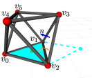
(a)

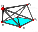
(b)

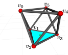
(c)

Figure 19: A VTT in octahedron configuration executes a single rolling locomotion step. (a) Initially node $v_{0}$, $v_{1}$, and $v_{2}$ forms the support polygon shown as the aqua region ($\blacktriangle$), and the center of mass projected onto the ground ($\bullet$) is within this support polygon. The truss wants to roll from its current support polygon to an adjacent support polygon formed by node $v_{1}$, $v_{2}$, and the new tipping location. (b) $v_{3}$ and $v_{5}$ are moved so that the support polygon is expanded and the center of mass projected onto the ground is on member $(v_{1},v_{2})$. (c) $v_{0}$ and $v_{4}$ are moved to their destinations to finish this locomotion step, and the center of mass projected onto the ground is within the new support polygon formed by node $v_{1}$, $v_{2}$, and $v_{3}$.

VII-A Truss Polyhedron

The boundary representation of a VTT is modeled as a convex polyhedron which can be either pre-defined or computed from the set of node positions by the convex hull [34]. Given a VTT $G=(V,E)$, its polyhedron representation can be fully defined as $P^{G}=(E^{G},F^{G})$ in which $F^{G}$ is the set of facets forming the boundary of this VTT and $E^{G}$ is the set of edges forming all facets. For example, the boundary representation of the VTT in Fig. 19a is an octahedron in which edge $(v_{1},v_{2})$ is incident to facet $(v_{1},v_{2},v_{3})$ and facet $(v_{0},v_{1},v_{2})$.

Suppose the set of edges forming a facet $f\in F^{G}$ is $E_{f}^{G}\subset E^{G}$, and $\forall e\in E_{f}^{G}$, the other incident facet of edge $e$ is $f^{e}\in F^{G}$. Assume $f\in F^{G}$ is the current support polygon and a single rolling locomotion step is equivalent to rotating the truss with respect to an edge of this facet $e\in E_{f}^{G}$ until the other incident facet of this edge $f^{e}$ becomes the new support polygon. An example is shown in Fig. 19. The motion of the robot from Fig. 19a to Fig. 19c is equivalent to rotating the truss with respect to the fixed edge $e=(v_{1},v_{2})$ until the support polygon becomes $f^{e}=(v_{1},v_{2},v_{3})$. This means the input command for each locomotion step can be simply an edge of the current support polygon, e.g., $(v_{1},v_{2})$ for the scenario in Fig. 19.

VII-B Locomotion Planning

Given a VTT $G=(V,E)$, its truss polyhedron model $P^{G}=(E^{G},F^{G})$ and its current support polygon $f\in F^{G}$ can be derived. Given a locomotion command $e\in f$, we can find $f^{e}$ and compute its normal vector $n_{f^{e}}$ pointing inward $P^{G}$ (e.g., vector $n$ for facet $(v_{1},v_{2},v_{3})$ in Fig. 19a), then the rotation angle $\alpha$ between $n_{f^{e}}$ and the normal vector of the ground $\left[0,0,1\right]^{\intercal}$ is simply

$$\alpha=\arccos\left(\frac{n_{f^{e}}\bullet\left[0,0,1\right]^{\intercal}}{\|n_{f^{e}}\|}\right)$$ (16)

The rotation axis is along edge $e=(v_{1}^{e},v_{2}^{e})$ and its direction can be determined by the right-hand rule. For the example shown in Fig. 19, the rotation axis is simply $\frac{q^{v_{1}}-q^{v_{2}}}{\|q^{v_{1}}-q^{v_{2}}\|}$. Assume the rotation axis is pointing from $v_{1}^{e}$ to $v_{2}^{e}$, then the rotation angle and the rotation axis determine a rotation matrix $R^{e}$, and for every node $v\in V\setminus\{v^{e}_{1},v^{e}_{2}\}$ during this locomotion process, its initial position $q_{i}^{v}$ is known as $q^{v}$ and its goal position $q_{g}^{v}$ can be derived as

$$q_{g}^{v}=R^{e}(q^{v}-q^{v_{1}^{e}})+q^{v_{1}^{e}}$$ (17)

Then we can make use of the approach presented in Section V-C to plan the motion for all involved nodes. The workspace can either be an known space or be set such that it can include the initial VTT and the goal VTT. Due to the stability constraint where the projected center of mass has to be within its support polygon, the planner will expand the support polygon by placing an additional node on the ground, so the center of mass can be moved in a larger range. An example of this non-impact rolling locomotion planning result is shown in Fig. 19. In this task, the initial support polygon is facet $(v_{0},v_{1},v_{2})$ and we want to roll the truss so that facet $(v_{1},v_{2},v_{3})$ becomes the new support polygon. The locomotion command is simply $(v_{1},v_{2})$, the rotation axis and the rotation angle can be computed as mentioned, and four nodes ($v_{0}$, $v_{3}$, $v_{4}$, $v_{5}$) have to move to new locations which can be derived from Eq. (17). Because of the stability constraint, node $v_{0}$ cannot be moved at the beginning, or the robot won’t be stable since there will be no support polygon. The planner chooses to move $v_{3}$ and $v_{5}$ first to expand the support polygon which is formed by node $v_{0}$, $v_{1}$, $v_{2}$, and $v_{3}$, and the center of mass is moved toward the target support polygon (Fig. 19b). The center of mass projected onto the ground is always within the initial support polygon. After the support polygon is expanded, $v_{0}$ and $v_{4}$ are moved, and, in the meantime, the projected center of mass enters the target support polygon (Fig. 19c).

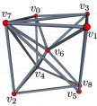
(a)

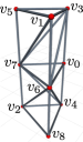
(b)

Figure 20: The motion task is to change the shape of a VTT from (a) a cubic truss for rolling locomotion to (b) a tower truss for shoring.

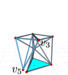
(a)

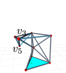
(b)

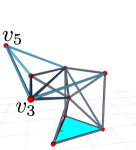
(c)

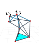
(d)

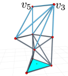
(e)

Figure 21: $v_{3}$ and $v_{5}$ firstly extend outward, and then move upward to their goal positions. The support polygon is formed by three nodes ($v_{2}$, $v_{4}$, $v_{5}$) on the ground shown as the aqua region ($\blacktriangle$) and the green dot ($\bullet$) is the center of mass represented on the ground.

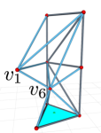
(a)

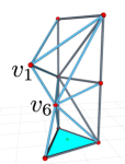
(b)

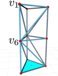
(c)

Figure 22: $v_{1}$ and $v_{6}$ can navigate to their goal positions easily since $\widehat{\mathcal{C}}_{\mathrm{free}}^{v_{1}}(q_{i}^{v_{1}})$ and $\widehat{\mathcal{C}}_{\mathrm{free}}^{v_{6}}(q_{i}^{v_{6}})$ almost cover the whole workspace.

VIII Test Scenarios

The motion planning framework is implemented in C++. Four example scenarios were conducted to measure the effectiveness of our approach. The performance of the reconfiguration framework is compared with the geometry reconfiguration approach in [15] and the topology reconfiguration approach in [16]. The performance of the locomotion framework is compared with the approach in [30] and [28]. All the comparisons are based on the test scenarios from these previous works. These experiments are also tested under different constraints and with different parameters to show the universality of our framework. All tests run on a laptop computer (Intel Core i7-8750H CPU, 16GB RAM) and the workspace is a cuboid.

VIII-A Geometry Reconfiguration

VIII-A1 Cube to Tower

The geometry reconfiguration planning test changes the cube shape of a VTT, Fig. 20a, to a tower shape, Fig. 20b. The constraints for this task are $\overline{L}_{\min}=$1.0\text{\,}\mathrm{m}$$, $\overline{L}_{\max}=$3.5\text{\,}\mathrm{m}$$, $\bar{\theta}_{\min}=$0.3\text{\,}\mathrm{rad}$$, and $\bar{\mu}_{\min}=0.1$.

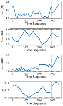
Figure 23: The minimum length ($L_{\min}$) and the maximum length ($L_{\max}$) of all moving edge modules, the minimum angle between every pair of edge modules ($\theta_{\min}$), and the motion manipulability ($\mu$) are measured throughout the geometry reconfiguration process in Fig. 22 and Fig. 22.

Four nodes $v_{1}$, $v_{3}$, $v_{5}$, and $v_{6}$ are involved in this motion task. These four nodes are separated into two groups $\{v_{3},v_{5}\}$ and $\{v_{1},v_{6}\}$ which are randomly selected. We first compute $\widehat{\mathcal{C}}_{\mathrm{free}}^{v_{3}}(q_{i}^{v_{3}})$ and $\widehat{\mathcal{C}}_{\mathrm{free}}^{v_{5}}(q_{i}^{v_{5}})$, and then do planning for these two nodes. The motions of node $v_{3}$ and $v_{5}$ are shown in Fig. 22. Most of the obstacle regions in this step are surrounded by the subspace $\widehat{\mathcal{C}}_{\mathrm{free}}^{v_{3}}(q_{i}^{v_{3}})$ and $\widehat{\mathcal{C}}_{\mathrm{free}}^{v_{5}}(q_{i}^{v_{5}})$, hence it is easier for them to extend outward first in order to navigate to the goal positions. This motion process moves the projected center of mass toward one edge of the support polygon but the planner can constrain the projected center of mass within the support polygon. After planning for $v_{3}$ and $v_{5}$, the truss is updated, and $\widehat{\mathcal{C}}_{\mathrm{free}}^{v_{1}}(q_{i}^{v_{1}})$ and $\widehat{\mathcal{C}}_{\mathrm{free}}^{v_{6}}(q_{i}^{v_{6}})$ are computed accordingly. Finally the planning for $v_{1}$ and $v_{6}$ finishes this motion task with the result shown in Fig. 22. For $v_{1}$ and $v_{6}$ in this updated truss, the enclosed subspace $\widehat{\mathcal{C}}_{\mathrm{free}}^{v_{1}}(q_{i}^{v_{1}})$ and $\widehat{\mathcal{C}}_{\mathrm{free}}^{v_{6}}(q_{i}^{v_{6}})$ almost covers the whole workspace so it is also easy for them to navigate to the goal positions. The minimum length ($L_{\min}$) and the maximum length ($L_{\max}$) of all moving edge modules, the minimum angle between every pair of edge modules ($\theta_{\min}$), and the motion manipulability ($\mu$) are shown in Fig. 23. Note that $L_{\min}$, $L_{\max}$, and $\mu$ are not necessarily to be continuous because nodes that are under control are changing. When moving $v_{3}$ and $v_{5}$, only compute the lengths of all blue members in Fig. 22 and compute the manipulability by setting $V_{C}=\{v_{3},v_{5}\}$ (before the blue dashed line in Fig. 23). Similarly, when moving $v_{1}$ and $v_{6}$, only compute the lengths of all blue members in Fig. 22 and compute the manipulability by setting $V_{C}=\{v_{1},v_{6}\}$ (after the blue dashed line in Fig. 23). This motion task is also demonstrated in [15] using the retraction-based RRT algorithm. This algorithm cannot solve this motion planning task in 100 trials unless an intermediate waypoint is manually specified to mitigate the narrow passage issue. The success rate for the planning from the initial to the waypoint is 99% and 98% from the waypoint to the goal. In comparison, with RRTConnect, our algorithm doesn’t need any additional waypoints, and we did 1000 trials and the mean running time is $4.29\text{\,}\mathrm{s}$ with a standard deviation of $1.99\text{\,}\mathrm{s}$ and the success rate is 100%. In these trials, the maximum running time is $7.56\text{\,}\mathrm{s}$ and the minimum is $1.01\text{\,}\mathrm{s}$. The mean computing time for configuration space is $1.04\text{\,}\mathrm{s}$ with a standard deviation of $0.38\text{\,}\mathrm{s}$, and the maximum computing time is $1.61\text{\,}\mathrm{s}$ and the minimum is $0.52\text{\,}\mathrm{s}$. The planing time is longer than that in our previous conference paper because more constraints are considered leading to more complicated configuration space computation and state validation.

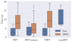
(a)

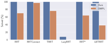
(b)

Figure 24: (a) The running time benchmark and (b) the solved percentage benchmark against standard OMPL planners.

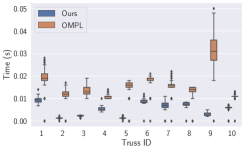
(a)

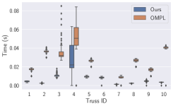
(b)

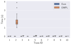
(c)

Figure 25: Benchmarks of randomly generated VTTs: (a) Group 1, (b) Group 2, (c) Group 3.

VIII-A2 Benchmark Test

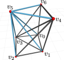
(a)

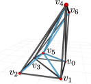
(b)

Figure 26: (a) A VTT is constructed from 18 edge modules with 6 nodes. (b) The goal is to move $v_{5}$ from its initial position to a position inside the truss.

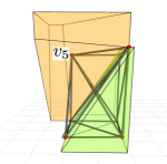
Figure 27: $\mathcal{C}_{\mathrm{free}}^{v_{5}}(q_{i}^{v_{5}})$ is the yellow space on the upper left and $\mathcal{C}_{\mathrm{free}}^{v_{5}}(q_{g}^{v_{5}})$ is the green space on the lower right. They are not connected and are separated by the obstacle region generated from edge $(v_{3},v_{4})$.

The performance of our framework is tested rigorously with several benchmarks. We first test the task shown in Fig. 20 and compare the performance with standard OMPL planners. We use the Flexible Collision Library (FCL) [35] for collision detection. In a VTT, every node is modeled as a sphere and every member is modeled as a cylinder. For standard OMPL planners, we have to set much smaller resolution at which state validity needs to be verified in order to ensure the motion does not skip over self-collision. Here we compare our planner with standard OMPL planners using several commonly used sampling-based planning approaches. The benchmark is shown in Fig. 24. Our planner can solve the task faster and also achieve higher success rate (100% except for using Lazy RRT and standard OMPL using Lazy RRT cannot find a solution). For optimal (RRT*) or near-optimal (LBTRRT) version of RRT, our planner also shows better performance in terms of success rate.

This benchmark shows our planner outperforms standard OMPL planners. The configuration space calculation significantly benefits the sampling-based planning phase in the following. First, both the maximum length of a motion to be added when searching and the resolution to validate state can be large because we have better way to validate motions. Second, our planner doesn’t heavily rely on the sampling-based planners. In our test, we set the maximum running time of the sampling-based planners to be only $2\text{\,}\mathrm{s}$ for our planner, but we need to set this parameter to be $20\text{\,}\mathrm{s}$ for standard OMPL planners in order to achieve higher success rate. Also some specific sampling-based planners, such as Transition-based RRT (TRRT), can have much better performance. Lazy RRT performs badly for truss robots. OMPL cannot solve this task and our planner can only achieve 8% success rate. This is because Lazy RRT is optimistic and attempts to find a solution as soon as possible without checking collision. Once a solution is found, validity checking is applied, and if collisions are found, the invalid path segments are removed and the search process is continued. However, VTT robots have a high probability of self-collision.

TABLE I: Random Truss Test

Group	# of Nodes	# of Members	# of Moving Nodes
1	6	12	$\leq 2$
2	8	15	$\leq 3$
3	9	20	$\leq 4$

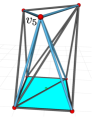
(a)

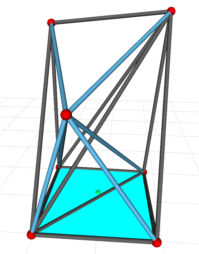
(b)

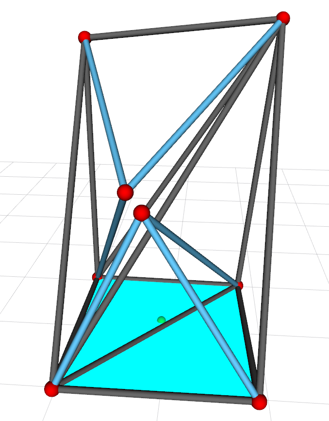
(c)

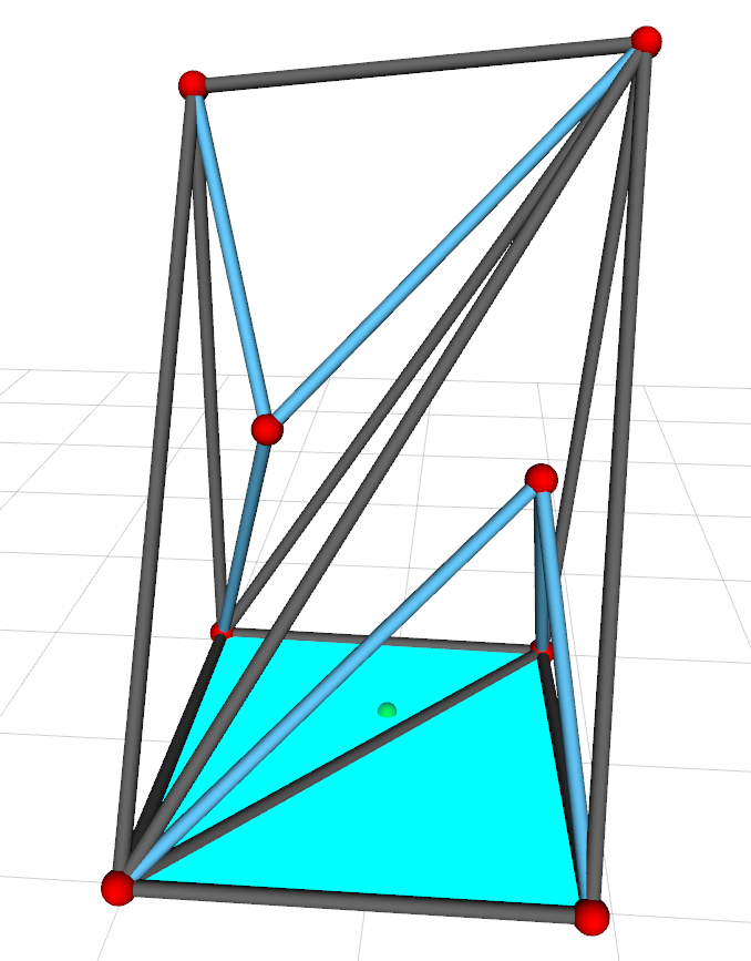
(d)

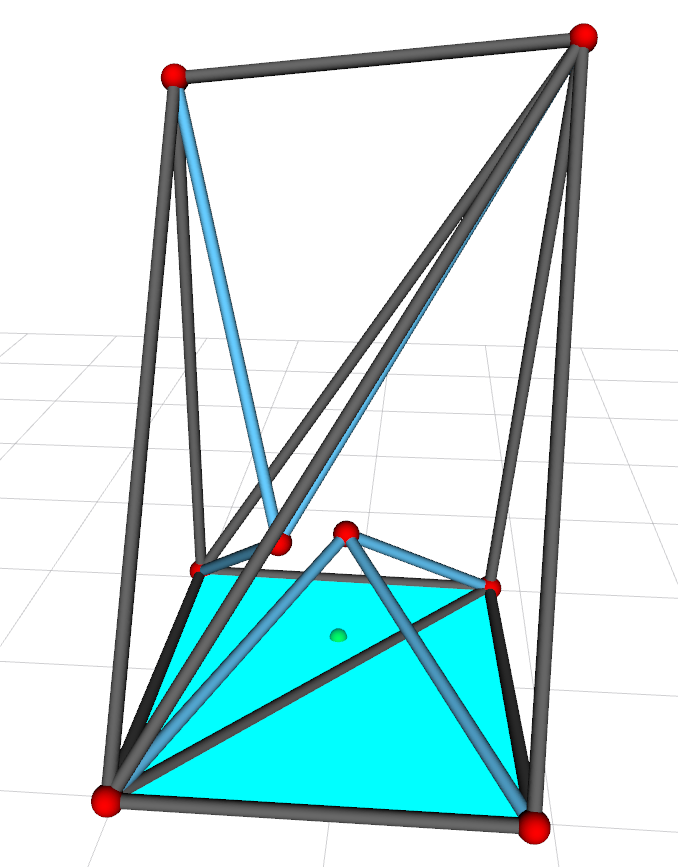
(e)

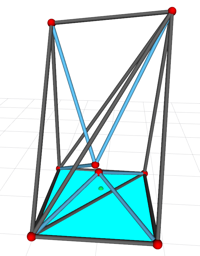
(f)

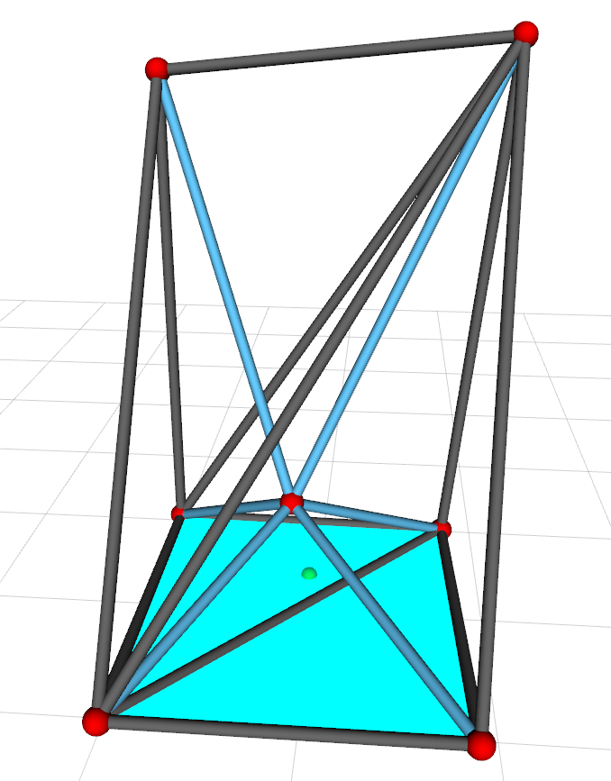
(g)

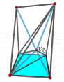
(h)

Figure 28: The sequence to move $v_{5}$ from $q_{i}^{v_{5}}$ to $q_{g}^{v_{5}}$ is shown. The support polygon is the aqua region ($\blacksquare$) and the green dot ($\bullet$) is the center of mass represented on the ground. (a) — (b) First move $v_{5}$ to a new location. (c) Split $v_{5}$ into a pair. (d) — (e) Move these two newly generated nodes in different directions to go around the edge module $(v_{3},v_{4})$. (f) — (h) Merge them into an individual node and move this node to $q_{g}^{v_{5}}$.

We also randomly generate three groups of trusses in different sizes and randomly generate motion goals shown in Table I. For every truss, we randomly select the nodes to move with randomly generated goals. In order to ensure valid goals (without topology reconfiguration), we compute the free space of every moving node and sample a goal inside this free space, which may lead to easy tasks because the free space for a group of nodes is larger than the union of the free space of every individual node in the group. Here we mainly compare the running time of the sampling-based planning phase using RRTConnect and the result (Fig. 25) shows that the configuration space computation can greatly improve the efficiency because our approach generates samples in a much smaller space. The success rates of both our planner and OMPL planner are 100% for most of the tests except for VTT 6 in Group 2 and VTT 4 in Group 3 in which OMPL cannot solve the task.

VIII-B Topology Reconfiguration

VIII-B1 Scenario 1

The VTT configuration used for this topology reconfiguration example is shown in Fig. 26a. The constraints for this task are $\overline{L}_{\min}=$1.0\text{\,}\mathrm{m}$$, $\overline{L}_{\max}=$5.0\text{\,}\mathrm{m}$$, $\bar{\theta}_{\min}=$0.2\text{\,}\mathrm{rad}$$, and $\bar{\mu}_{\min}=0.1$.

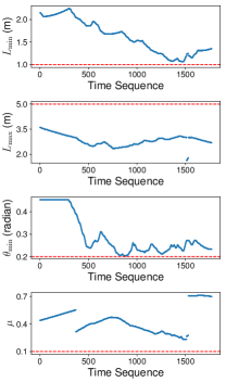
Figure 29: The minimum length ($L_{\min}$) and the maximum length ($L_{\max}$) of all moving edge modules, the minimum angle between every pair of edge modules ($\theta_{\min}$), and the motion manipulability ($\mu$) are measured throughout the topology reconfiguration process in Fig. 28.

The motion task is to move $v_{5}$ from its initial position $q_{i}^{v_{5}}$ to a goal position $q_{g}^{v_{5}}$ (Fig. 26b). This motion cannot be executed with only geometry reconfiguration because $\mathcal{C}_{\mathrm{free}}^{v_{5}}(q_{i}^{v_{5}})$ and $\mathcal{C}_{\mathrm{free}}^{v_{5}}(q_{g}^{v_{5}})$ shown in Fig. 27 are separated by the obstacle region generated from edge module $(v_{3},v_{4})$. For this task, the minimum distance between two nodes is $d_{\min}=$1.0\text{\,}\mathrm{m}$$ and $N_{\max}$ is constrained to be greater than or equal to $3$, namely it is expected to have at least 3 samples for every enclosed subspace, and the maximum number of iterations $K=5N_{\max}$.

With our topology reconfiguration planning algorithm (Algorithm 4), one pair of Split and Merge actions is sufficient. $v_{5}$ is moved to a new location, then split into a pair of nodes ($v^{\prime}_{5}$ and $v^{\prime\prime}_{5}$) so that both of these two newly generated nodes can navigate to $\mathcal{C}_{\mathrm{free}}^{v_{5}}(q_{g}^{v_{5}})$ and merge into a single node. Then the geometry motion planning is used to plan the motions of $v^{\prime}_{5}$ and $v^{\prime\prime}_{5}$ and control them to the target positions for merging. Finally, merge them back to an individual node and then move the node to $q_{g}^{v_{5}}$. The detailed process is shown in Fig. 28. The minimum length ($L_{\min}$) and the maximum length ($L_{\max}$) of all moving edge modules, the minimum angle between every pair of edge modules ($\theta_{\min}$), and the motion manipulability ($\mu$) are shown in Fig. 29.

This motion task has been solved in [16] with the graph search algorithm exploring 8146 VTT configurations with a more complex action model in order to find a valid sequence of motion actions. With the proposed framework, the free space of $v_{5}$ is partitioned into 53 enclosed subspaces and it takes on average $56.61\text{\,}\mathrm{s}$ to solve this motion task when using the first transition model with a standard deviation of $5.65\text{\,}\mathrm{s}$ in 1000 trials, including the enclosed subspace computation, topology reconfiguration planning, and two-node geometry reconfiguration planning, and the success rate is 100%. In these trials, the maximum planning time is $77.88\text{\,}\mathrm{s}$ and the minimum is $38.97\text{\,}\mathrm{s}$. With the transition model based on the group free space, the average planning time for 1000 trials can be as fast as $21.99\text{\,}\mathrm{s}$ with a standard deviation of $0.67\text{\,}\mathrm{s}$, and the success rate is 100%. In these trials, the maximum planning time is $24.01\text{\,}\mathrm{s}$ and the minimum is $24.45\text{\,}\mathrm{s}$.

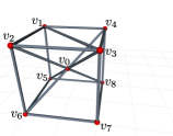
(a)

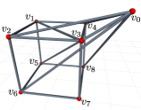
(b)

Figure 30: (a) A VTT is constructed from 19 members with 9 nodes. (b) The task is to move $v_{0}$ from its initial position to a position outside the cubic truss.

Figure 31: $v$ has to move from $\mathcal{C}_{\mathrm{free}}^{v}(q_{i}^{v})$ that is the yellow enclosed subspace to the green enclosed subspace, and then $\mathcal{C}_{\mathrm{free}}^{v}(q_{g}^{v})$ that is the blue enclosed subspace.

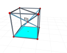
(a)

(b)

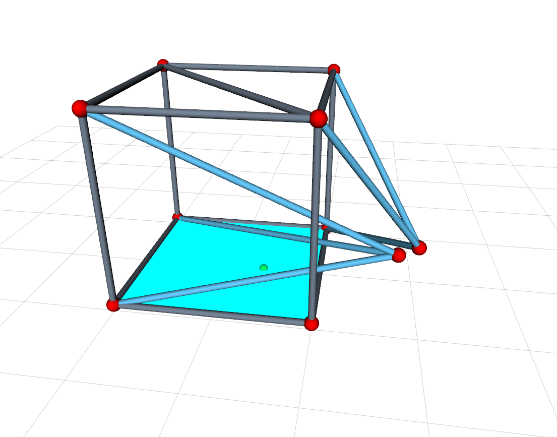
(c)

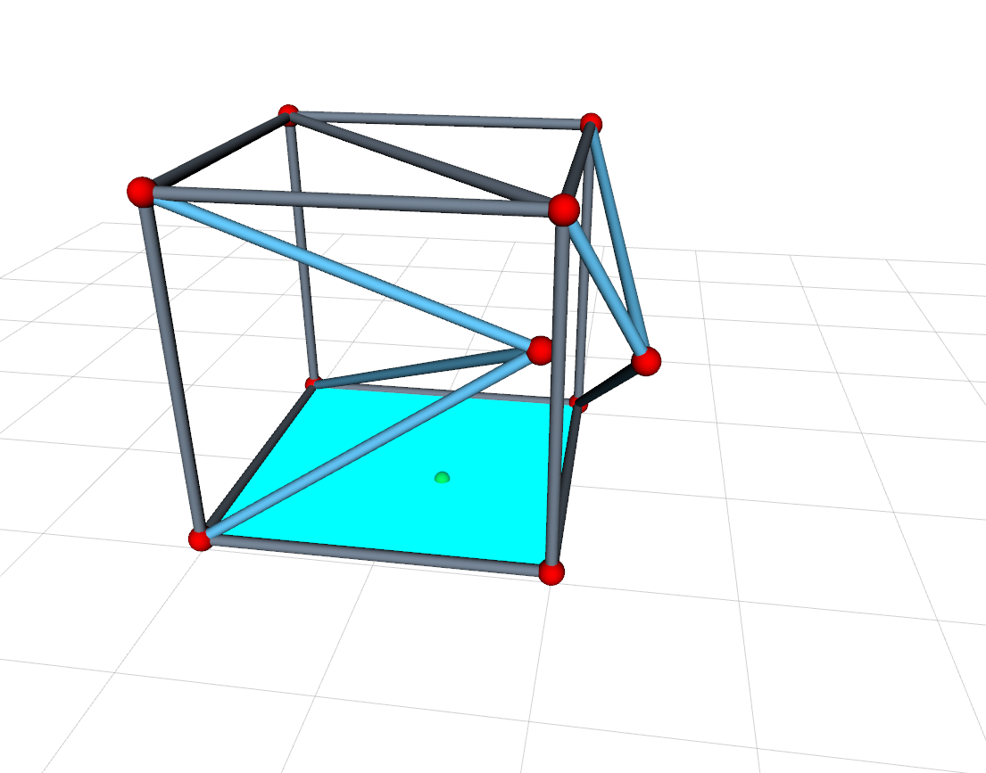
(d)

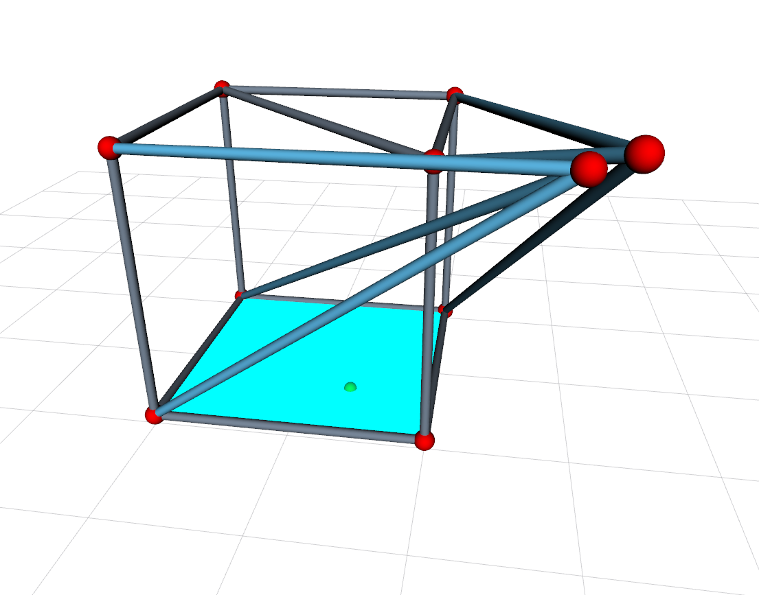
(e)

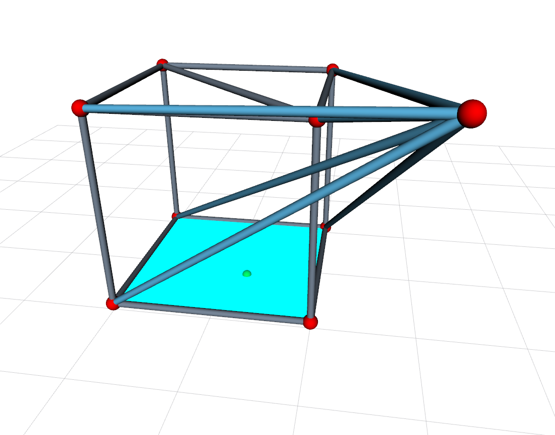
(f)

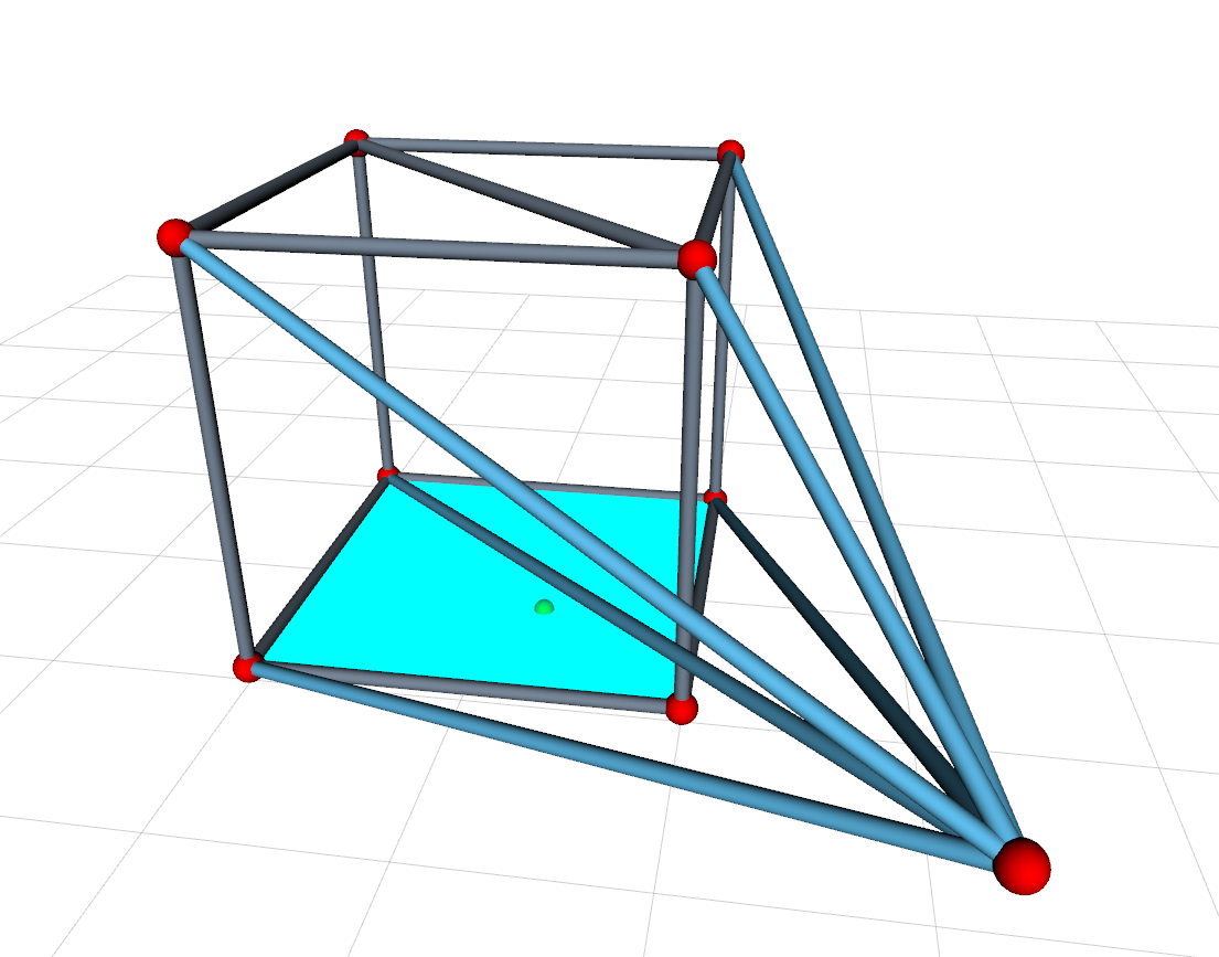
(g)

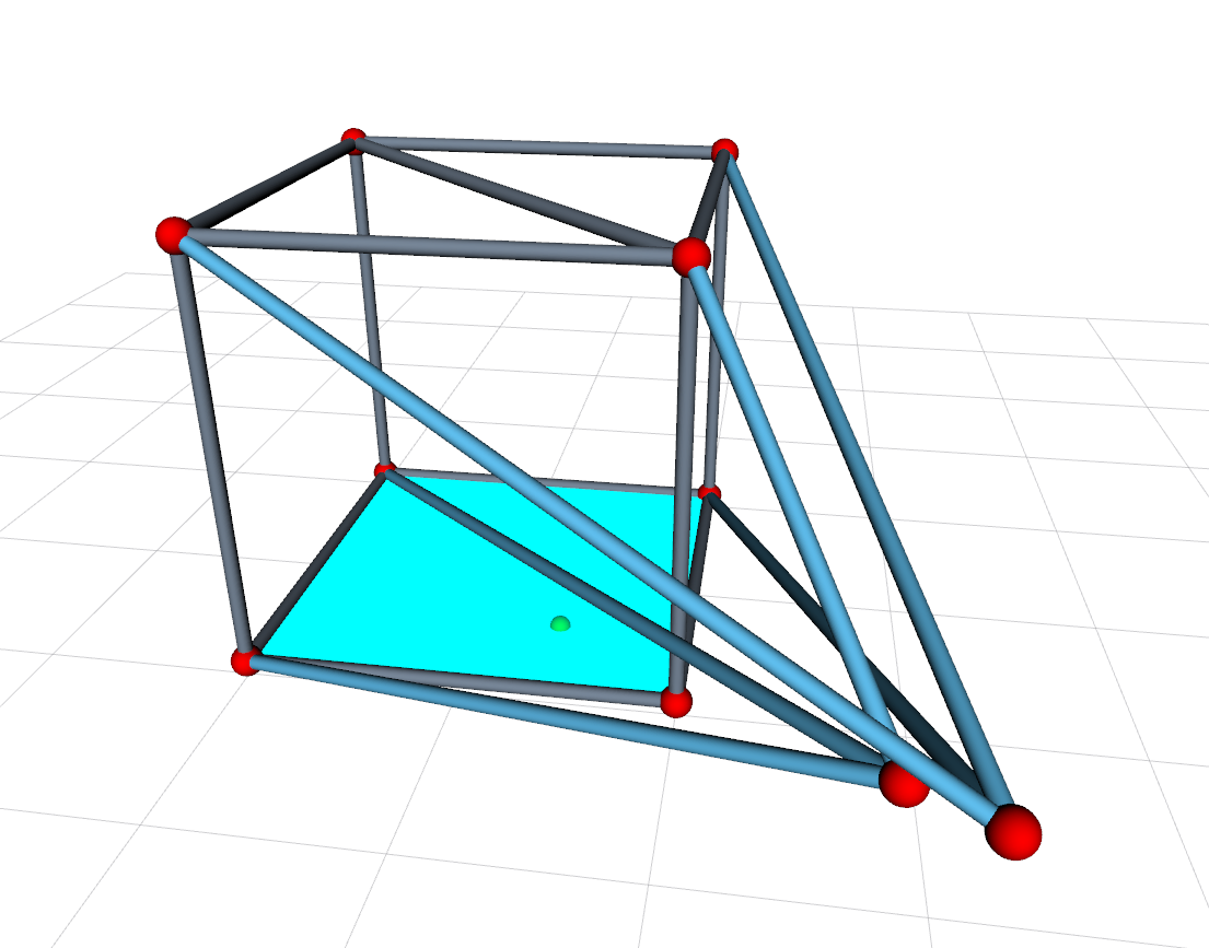
(h)

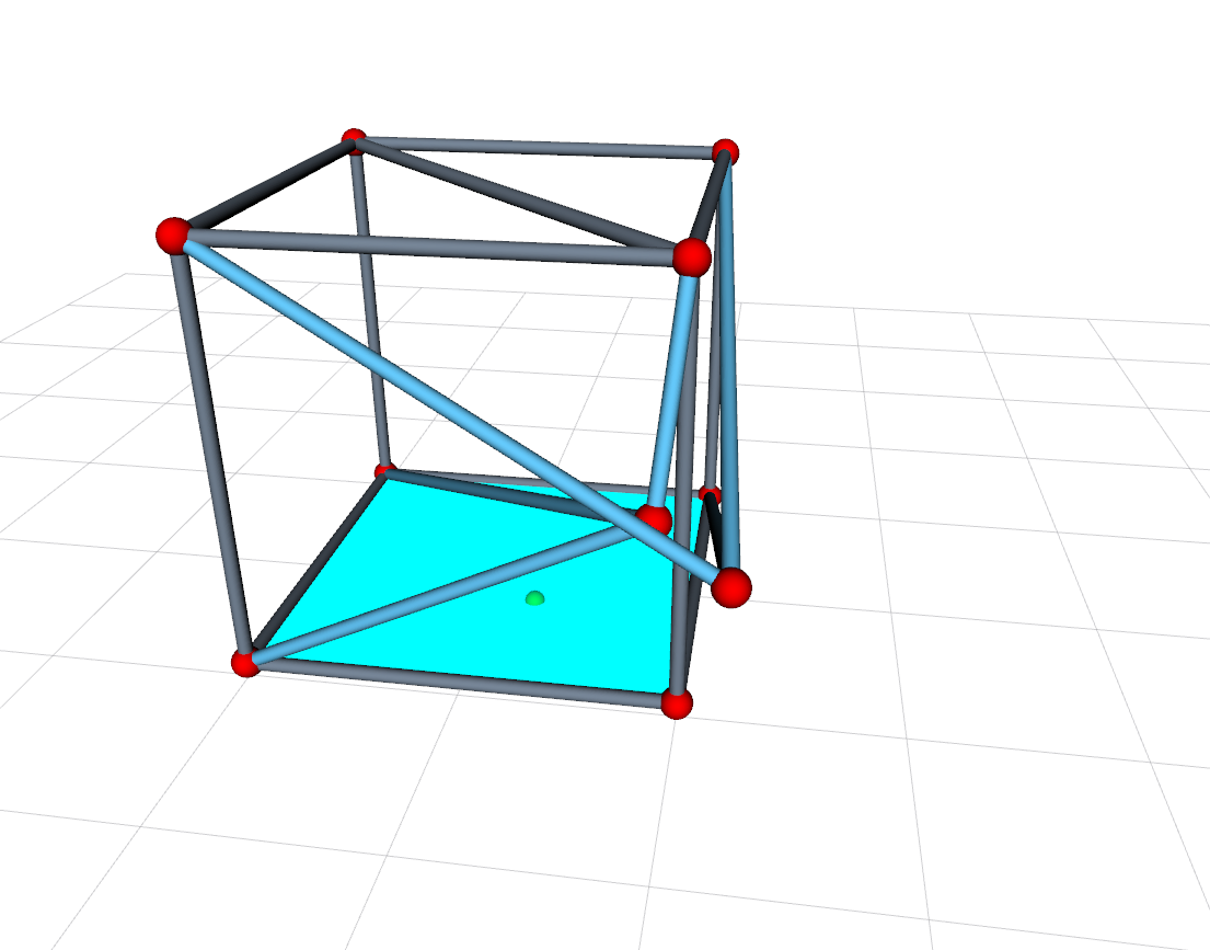
(i)

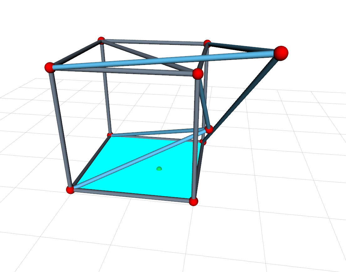
(j)

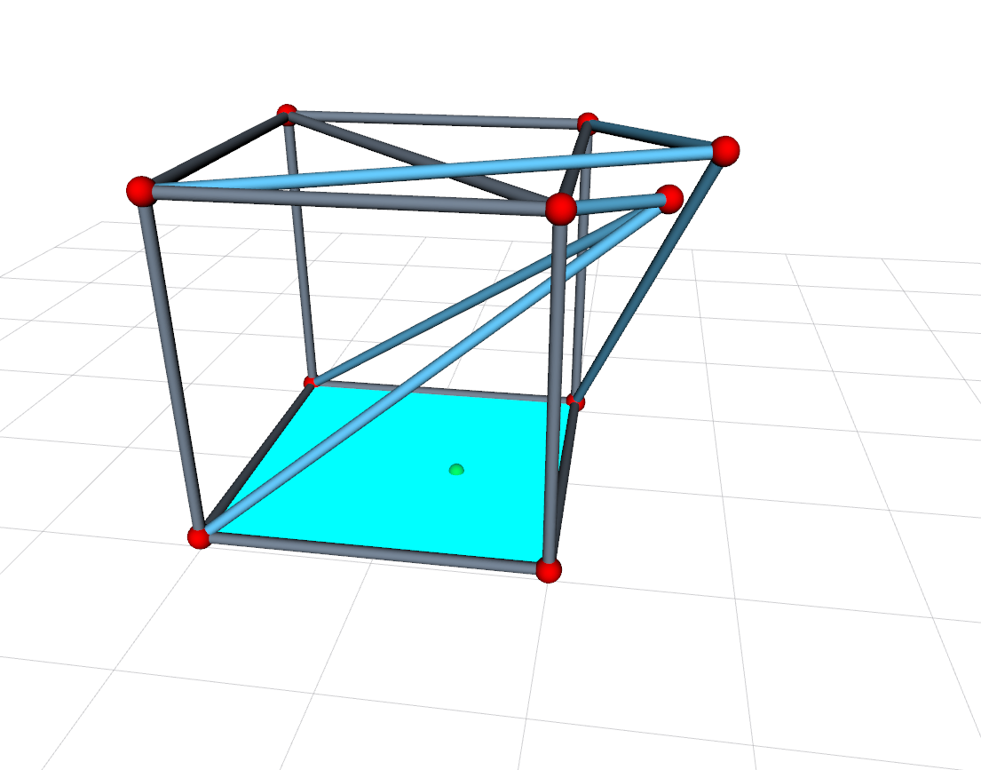
(k)

(l)

Figure 32: The sequence to move $v_{0}$ from $q_{i}^{v_{0}}$ to $q_{g}^{v_{0}}$ by traversing three enclosed subspaces in $\mathcal{C}_{\mathrm{free}}^{v}$ is shown. The support polygon is the aqua region ($\blacksquare$) and the green dot ($\bullet$) is the center of mass represented on the ground. (a) — (b) Move node $v_{0}$ to traverse the plane formed by node $v_{3}$, $v_{4}$, $v_{7}$, and $v_{8}$. (c) Split the node into a pair here so that both newly generated nodes can move around edge module $(v_{3},v_{7})$ while avoiding singular configuration. (d) — (f) Two newly generated nodes are moved to a location inside the green enclosed subspace and merge. (g) — (h) Move the merged node to a new location and split it in a different way to generate two new nodes. (i) — (l) One node traverses the space inside the cubic truss to go to the blue enclosed subspace, and the other node moves upward. Then these two nodes merge at a location inside the blue enclosed subspace and then move to the target location.

VIII-B2 Scenario 2

Another motion task in which topology reconfiguration actions are involved is shown in Fig. 30 that is to move $v_{0}$ from a position $q_{i}^{v_{0}}$ inside the cubic truss (Fig. 30a) to a new position $q_{g}^{v_{0}}$ (Fig. 30b). The constraints for this task are $\overline{L}_{\min}=$0.5\text{\,}\mathrm{m}$$, $\overline{L}_{\max}=$5.0\text{\,}\mathrm{m}$$, $\bar{\theta}_{\min}=$0.15\text{\,}\mathrm{rad}$$, and $\bar{\mu}_{\min}=0.1$.

In this task, $q_{i}^{v_{0}}$ and $q_{g}^{v_{0}}$ are in two separated enclosed subspaces, and one solution is to apply topology reconfiguration actions twice to traverse three enclosed subspaces in $\mathcal{C}_{\mathrm{free}}^{v}$ shown in Fig. 31. For this task, $d_{\min}=0.5$, $N_{\max}$ is constrained to be greater than or equal to $3$, and $K=8N_{\max}$.

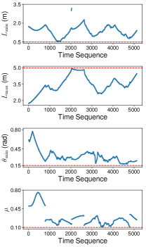
Figure 33: The minimum length ($L_{\min}$) and the maximum length ($L_{\max}$) of all moving edge modules, the minimum angle between every pair of edge modules ($\theta_{\min}$), and the motion manipulability ($\mu$) are measured throughout the topology reconfiguration process in Fig. 32.

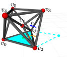
(a)

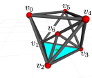
(b)

Figure 34: The locomotion task is to roll the truss from (a) to (b).

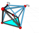
(a)

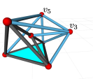
(b)

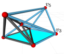
(c)

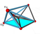
(d)

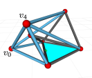
(e)

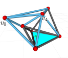
(f)

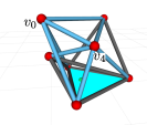
(g)

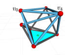
(h)

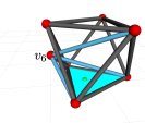
(i)

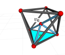
(j)

Figure 35: The planned motion for this locomotion task is shown. (a) — (c) Move node $v_{3}$ and $v_{5}$ to first expand the support polygon that is the aqua region. (d) Move $v_{0}$ and $v_{4}$ to move the center of mass represented on the ground ($\bullet$) toward the target support polygon. (e) — (h) Once the center of mass represented on the ground is inside the target support polygon, lift $v_{0}$ and move both $v_{0}$ and $v_{4}$ to their target locations. (i) — (j) Finally move $v_{6}$ to its target location to finish the locomotion process.

The detailed planning result is shown in Fig. 32. We first move the node $v_{0}$ to a location outside the cubic truss (Fig. 32a — Fig. 32b), and then split it into two. If the node is split inside the cubic truss, there is no way to merge them inside the green enclosed subspace (Fig. 32f) because one node has to traverse a region formed by node $v_{3}$, $v_{4}$, $v_{7}$, and $v_{8}$ resulting in singular configurations. After this Split action, do geometry reconfiguration planning to control them to the green enclosed subspace (Fig. 32c — Fig. 32e) and merge them back. Then move the node to a different location inside the green enclosed subspace (Fig. 32g) and then split the node in a different way (Fig. 32h) in order to navigate these two nodes to $\mathcal{C}_{\mathrm{free}}^{v}(q_{g}^{v_{0}})$ (Fig. 32i — Fig. 32k) and merge them back. Eventually move the node to $q_{g}^{v_{0}}$ (Fig. 32l). The minimum length ($L_{\min}$) and the maximum length ($L_{\max}$) of all moving edge modules, the minimum angle between every pair of edge modules ($\theta_{\min}$), and the motion manipulability ($\mu$) are shown in Fig. 33. Using the strict transition model, the average planning time is $319.83\text{\,}\mathrm{s}$ with a standard deviation being $21.31\text{\,}\mathrm{s}$ in 1000 trials, and the success rate is 74%. In these trials, the maximum planning time is $392.47\text{\,}\mathrm{s}$ and the minimum is $172.05\text{\,}\mathrm{s}$. The search space is larger and more samples are generated in order to find the sequence of topology reconfiguration actions which consumes more time. All the failures are from the graph search phase, and more samples can solve this issue but also make the search process more time consuming. With the same parameters, when using the other transition model based on the group free space, the average planning time is $86.48\text{\,}\mathrm{s}$ with a standard deviation being $2.05\text{\,}\mathrm{s}$ in 1000 trials, and the success rate is 95.9%. The maximum planning time is $92.85\text{\,}\mathrm{s}$ and the minimum planning time is $79.98\text{\,}\mathrm{s}$. The performance is improved a lot. All the failures in these trials are from the path planning for a group of node, namely even the transition model between two enclosed subspace is valid, it is not guaranteed for the planner to find the solution. Similar to the geometry reconfiguration test, it also takes more time for the topology reconfiguration planning compared with our previous conference paper. This is because the planner needs to validate Split actions and generate enough samples to span the space, and the transition model is also more complex.

VIII-C Locomotion

The VTT used for the locomotion test is shown in Fig. 34a that is an octahedron with three additional edge modules internally. The constraints for this locomotion task are $\overline{L}_{\min}=$0.3\text{\,}\mathrm{m}$$, $\overline{L}_{\max}=$2.3\text{\,}\mathrm{m}$$, $\bar{\theta}_{\min}=$0.3\text{\,}\mathrm{rad}$$, and $\bar{\mu}_{\min}=0.1$. The task is to roll this VTT to an adjacent support polygon shown in Fig. 34b, and the locomotion command is $(v_{1},v_{2})$. Five nodes ($v_{0}$, $v_{3}$, $v_{4}$, $v_{5}$, and $v_{6}$) are involved in this process and their goal locations can be computed by Eq. (17).

The detailed locomotion process is shown in Fig. 35. Five nodes are divided into three groups and the whole process is also divided into three phases automatically. In the first phase, $v_{3}$ and $v_{5}$ are moved to expand the support polygon (Fig. 35b and Fig. 35c). Then $v_{0}$ and $v_{4}$ are moved gradually to move the center of mass toward the adjacent support polygon shown in Fig. 35d. Once the center of mass represented on the ground is inside the target support polygon, $v_{0}$ can be lifted off the ground and both $v_{0}$ and $v_{4}$ can be moved to their target locations (Fig. 35e—Fig. 35h). Finally, move node $v_{6}$ to its target location shown in Fig. 35j to finish the whole process.

The minimum length ($L_{\min}$) and the maximum length ($L_{\max}$) of all moving edge modules, the minimum angle between every pair of edge modules ($\theta_{\min}$), and the motion manipulability ($\mu$) are shown in Fig. 36. This rolling step is tested with 1000 trials and the average planning time is $8.30\text{\,}\mathrm{s}$ with the standard deviation being $5.94\text{\,}\mathrm{s}$ in 1000 trials, and the success rate is 100%. In these trials, the maximum planning time is $24.50\text{\,}\mathrm{s}$ and the minimum planning time is $0.47\text{\,}\mathrm{s}$. The locomotion of this VTT is also tested in [30] and the performance comparison is shown in Table II. Our planner has better performance in terms of both efficiency and robustness.

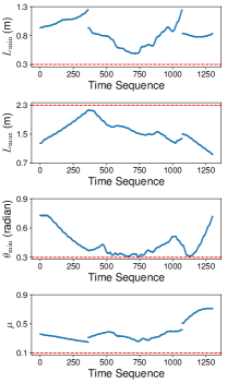
Figure 36: The minimum length ($L_{\min}$) and the maximum length ($L_{\max}$) of all moving edge modules, the minimum angle between every pair of edge modules ($\theta_{\min}$), and the motion manipulability ($\mu$) are measured throughout the locomotion process in Fig. 35.

TABLE II: Comparison with [30].

	Avg. Plan Time	Success Rate
Optimization	$18.84\text{\,}\mathrm{s}$	38.3% (820 trials)
Sampling-Based (Ours)	$8.30\text{\,}\mathrm{s}$	100% (1000 trials)

TABLE III: Comparison with [28].

	Avg. Plan Time	Success Rate
Optimization	$166\text{\,}\mathrm{s}$	Not provided
Sampling-Based (Ours)	$1.18\text{\,}\mathrm{s}$	100% (1000 trials)

An octahedron rolling gait is computed based on an optimization approach in [28]. Impacts are not considered in this approach and it takes $166\text{\,}\mathrm{s}$ to compute the whole process. The octahedron configuration is also tested with our framework and the comparison is shown in Table III. The solution (Fig. 19) can be derived as fast as $1.18\text{\,}\mathrm{s}$ in average with a standard deviation being $1.03\text{\,}\mathrm{s}$ in 1000 trials, and the success rate is 100%. In these trials, the maximum planning time is $3.44\text{\,}\mathrm{s}$ and the minimum is $0.10\text{\,}\mathrm{s}$.

IX Conclusion

A motion planning framework for variable topology truss robots is presented in this paper. Physical constraints such as joint limits, truss member diameter, static stability during locomotion, and motion manipulability are accounted for. An efficient algorithm to compute the obstacle regions and the free space of a group is developed so that sampling-based planners can be applied to solve the self-collision-free motion of multiple nodes. A fast algorithm to compute all enclosed subspaces in the free space of a node is presented so that we can verify whether topology reconfiguration actions are needed. A sample generation method is introduced to efficiently provide valid topology reconfiguration actions over a wide space. With our graph search algorithm, a sequence of topology reconfiguration actions can then be computed with geometry reconfiguration planning for a group of nodes, and the motion tasks requiring topology reconfiguration can then be solved efficiently. A non-impact rolling locomotion algorithm is presented to move an arbitrary VTT easily by a simple command with our efficient geometry reconfiguration planner. Our locomotion algorithm outperforms other approaches in terms of efficiency and robustness. Future work includes motion planning in more complex environments, such as locomotion in complex terrains, and the exploration of heuristic functions for truss robots to speed up the planning.

References

- [1] M. Yim, W. Shen, B. Salemi, D. Rus, M. Moll, H. Lipson, E. Klavins, and G. S. Chirikjian, “Modular self-reconfigurable robot systems [grand challenges of robotics],” IEEE Robotics Automation Magazine, vol. 14, no. 1, pp. 43–52, March 2007.
- [2] J. W. Suh, S. B. Homans, and M. Yim, “Telecubes: Mechanical design of a module for self-reconfigurable robotics,” in Proceedings 2002 IEEE International Conference on Robotics and Automation (Cat. No.02CH37292), vol. 4, May 2002, pp. 4095–4101 vol.4.
- [3] K. Gilpin, K. Kotay, D. Rus, and I. Vasilescu, “Miche: Modular shape formation by self-disassembly,” The International Journal of Robotics Research, vol. 27, no. 3-4, pp. 345–372, 2008.
- [4] M. Yim, D. G. Duff, and K. D. Roufas, “PolyBot: A modular reconfigurable robot,” in Proceedings 2000 ICRA. Millennium Conference. IEEE International Conference on Robotics and Automation. Symposia Proceedings (Cat. No.00CH37065), vol. 1, April 2000, pp. 514–520 vol.1.
- [5] M. Yim, P. White, M. Park, and J. Sastra, “Modular self-reconfigurable robots,” in Encyclopedia of Complexity and Systems Science, R. A. Meyers, Ed. New York, NY: Springer New York, 2009, pp. 5618–5631.
- [6] B. Salemi, M. Moll, and W. Shen, “SUPERBOT: A deployable, multi-functional, and modular self-reconfigurable robotic system,” in 2006 IEEE/RSJ International Conference on Intelligent Robots and Systems, Oct 2006, pp. 3636–3641.
- [7] S. Murata, E. Yoshida, A. Kamimura, H. Kurokawa, K. Tomita, and S. Kokaji, “M-TRAN: Self-reconfigurable modular robotic system,” IEEE/ASME Transactions on Mechatronics, vol. 7, no. 4, pp. 431–441, Dec 2002.
- [8] C. Liu, M. Whitzer, and M. Yim, “A distributed reconfiguration planning algorithm for modular robots,” IEEE Robotics and Automation Letters, vol. 4, no. 4, pp. 4231–4238, Oct 2019.
- [9] K. Miura, “Design and operation of a deployable truss structure,” in NASA. Goddard Space Flight Center The 18th Aerospace Mech. Symp., Greenbelt, Maryland, may 1984, pp. 49–63.
- [10] G. J. Hamlin and A. C. Sanderson, “TETROBOT: A modular approach to parallel robotics,” IEEE Robotics Automation Magazine, vol. 4, no. 1, pp. 42–50, March 1997.
- [11] A. Lyder, R. F. M. Garcia, and K. Stoy, “Mechanical design of Odin, an extendable heterogeneous deformable modular robot,” in 2008 IEEE/RSJ International Conference on Intelligent Robots and Systems, Sep. 2008, pp. 883–888.
- [12] N. Usevitch, Z. Hammond, S. Follmer, and M. Schwager, “Linear actuator robots: Differential kinematics, controllability, and algorithms for locomotion and shape morphing,” in 2017 IEEE/RSJ International Conference on Intelligent Robots and Systems (IROS), Sep. 2017, pp. 5361–5367.
- [13] E. Komendera and N. Correll, “Precise assembly of 3D truss structures using MLE-based error prediction and correction,” The International Journal of Robotics Research, vol. 34, no. 13, pp. 1622–1644, 2015.
- [14] A. Spinos, D. Carroll, T. Kientz, and M. Yim, “Variable topology truss: Design and analysis,” in 2017 IEEE/RSJ International Conference on Intelligent Robots and Systems (IROS), Sep. 2017, pp. 2717–2722.
- [15] S. Jeong, B. Kim, S. Park, E. Park, A. Spinos, D. Carroll, T. Tsabedze, Y. Weng, T. Seo, M. Yim, F. C. Park, and J. Kim, “Variable topology truss: Hardware overview, reconfiguration planning and locomotion,” in 2018 15th International Conference on Ubiquitous Robots (UR), June 2018, pp. 610–615.
- [16] C. Liu and M. Yim, “Reconfiguration motion planning for variable topology truss,” in 2019 IEEE/RSJ International Conference on Intelligent Robots and Systems (IROS), Nov 2019, pp. 1941–1948.
- [17] C. Liu, S. Yu, and M. Yim, “Motion planning for variable topology truss modular robot,” in Proceedings of Robotics: Science and Systems, Corvalis, Oregon, USA, July 2020.
- [18] C. Liu, S. Yu, and M. Yim, “A fast configuration space algorithm for variable topology truss modular robots,” in 2020 IEEE International Conference on Robotics and Automation (ICRA), May 2020, pp. 8260–8266.
- [19] A. Casal and M. Yim, “Self-reconfiguration planning for a class of modular robots,” in Sensor Fusion and Decentralized Control in Robotic Systems II, G. T. McKee and P. S. Schenker, Eds., vol. 3839, International Society for Optics and Photonics. SPIE, 1999, pp. 246 – 257.
- [20] Z. Butler, K. Kotay, D. Rus, and K. Tomita, “Generic decentralized control for lattice-based self-reconfigurable robots,” The International Journal of Robotics Research, vol. 23, no. 9, pp. 919–937, 2004.
- [21] F. Hou and W.-M. Shen, “Graph-based optimal reconfiguration planning for self-reconfigurable robots,” Robotics and Autonomous Systems, vol. 62, no. 7, pp. 1047 – 1059, 2014.
- [22] S. K. Agrawal, L. Kissner, and M. Yim, “Joint solutions of many degrees-of-freedom systems using dextrous workspaces,” in Proceedings 2001 ICRA. IEEE International Conference on Robotics and Automation (Cat. No.01CH37164), vol. 3, May 2001, pp. 2480–2485 vol.3.
- [23] M. Fromherz, T. Hogg, Y. Shang, and W. Jackson, “Modular robot control and continuous constraint satisfaction,” in Proceedings of IJCAI Workshop on Modelling and Solving Problems with Contraints, Seatle, WA, 2001, pp. 47–56.
- [24] C. Liu and M. Yim, “A quadratic programming approach to manipulation in real-time using modular robots,” The International Journal of Robotic Computing, vol. 3, no. 1, pp. 121–145, 2021.
- [25] C. Liu, S. Yu, and M. Yim, “Shape morphing for variable topology truss,” in 2019 16th International Conference on Ubiquitous Robots (UR), Jeju, Korea, June 2019.
- [26] Woo Ho Lee and A. C. Sanderson, “Dynamic rolling locomotion and control of modular robots,” IEEE Transactions on Robotics and Automation, vol. 18, no. 1, pp. 32–41, Feb 2002.
- [27] M. Abrahantes, L. Nelson, and P. Doorn, “Modeling and gait design of a 6-tetrahedron walker robot,” in 2010 42nd Southeastern Symposium on System Theory (SSST), March 2010, pp. 248–252.
- [28] N. S. Usevitch, Z. M. Hammond, and M. Schwager, “Locomotion of linear actuator robots through kinematic planning and nonlinear optimization,” IEEE Transactions on Robotics, pp. 1–18, 2020.
- [29] S. Park, E. Park, M. Yim, J. Kim, and T. W. Seo, “Optimization-based nonimpact rolling locomotion of a variable geometry truss,” IEEE Robotics and Automation Letters, vol. 4, no. 2, pp. 747–752, April 2019.
- [30] S. Park, J. Bae, S. Lee, M. Yim, J. Kim, and T. Seo, “Polygon-based random tree search planning for variable geometry truss robot,” IEEE Robotics and Automation Letters, vol. 5, no. 2, pp. 813–819, April 2020.
- [31] L. Kettner, “Using generic programming for designing a data structure for polyhedral surfaces,” Computational Geometry, vol. 13, no. 1, pp. 65–90, 1999.
- [32] F. Collins and M. Yim, “Design of a spherical robot arm with the spiral zipper prismatic joint,” in 2016 IEEE International Conference on Robotics and Automation (ICRA), May 2016, pp. 2137–2143.
- [33] I. A. Sucan, M. Moll, and L. E. Kavraki, “The open motion planning library,” IEEE Robotics Automation Magazine, vol. 19, no. 4, pp. 72–82, Dec 2012.
- [34] C. B. Barber, D. P. Dobkin, and H. Huhdanpaa, “The quickhull algorithm for convex hulls,” ACM Trans. Math. Softw., vol. 22, no. 4, p. 469–483, Dec. 1996.
- [35] J. Pan, S. Chitta, and D. Manocha, “FCL: A general purpose library for collision and proximity queries,” in 2012 IEEE International Conference on Robotics and Automation, 2012, pp. 3859–3866.