A graphical multi-fidelity Gaussian process model, with application to emulation of heavy-ion collisions

Abstract

With advances in scientific computing and mathematical modeling, complex scientific phenomena such as galaxy formations and rocket propulsion can now be reliably simulated. Such simulations can however be very time-intensive, requiring millions of CPU hours to perform. One solution is multi-fidelity emulation, which uses data of different fidelities to train an efficient predictive model which emulates the expensive simulator. For complex scientific problems and with careful elicitation from scientists, such multi-fidelity data may often be linked by a directed acyclic graph (DAG) representing its scientific model dependencies. We thus propose a new Graphical Multi-fidelity Gaussian Process (GMGP) model, which embeds this DAG structure (capturing scientific dependencies) within a Gaussian process framework. We show that the GMGP has desirable modeling traits via two Markov properties, and admits a scalable algorithm for recursive computation of the posterior mean and variance along at each depth level of the DAG. We also present a novel experimental design methodology over the DAG given an experimental budget, and propose a nonlinear extension of the GMGP via deep Gaussian processes. The advantages of the GMGP are then demonstrated via a suite of numerical experiments and an application to emulation of heavy-ion collisions, which can be used to study the conditions of matter in the Universe shortly after the Big Bang. The proposed model has broader uses in data fusion applications with graphical structure, which we further discuss.

Keywords: Computer experiments, Gaussian processes, graphical models, nuclear physics, multi-fidelity modeling.

1 Introduction

With breakthroughs in scientific computing, computer simulations are quickly replacing physical experiments in modern scientific and engineering problems. These simulations allow scientists to better understand complex scientific problems which may be prohibitively expensive or infeasible for full-scale physical experimentation. This shift to computer experimentation has found success in exciting applications, including cell adhesion simulation (Sung et al.,, 2020) and rocket design (Mak et al.,, 2018). Such computer experiments, however, can demand a hefty price in computing resources, requiring millions of CPU hours per run. One solution is emulation (Santner et al.,, 2019; Gramacy,, 2020): a handful of simulations are first run at carefully chosen design points, then an emulator model is fit to efficiently predict the expensive computer simulator. A popular emulator is the Gaussian process (GP) model (Gramacy,, 2020), which allows for closed-form expressions for prediction and uncertainty quantification.

As systems become more realistic and complex, computer experiments also become increasingly more expensive, and thus the simulation data needed to train an accurate emulator can be difficult to generate. One way to address this is multi-fidelity emulation. The idea is to collect data from the “high-fidelity” simulator, which is computationally expensive but provides a detailed representation of the modeled science, as well as data from “lower-fidelity” simulators, which make simplifying assumptions on the modeled science but can be performed quickly. One then fits a multi-fidelity emulator using all training data to predict the output from the high-fidelity simulator. The key advantage of multi-fidelity emulation is that, by leveraging information from cheaper lower-fidelity simulations to enhance predictions for the high-fidelity model, one can train a predictive model with much fewer high-fidelity simulations and thereby lower computational costs.

The development of multi-fidelity emulators is an active research area. A popular framework is the Kennedy-O’Hagan (KO) model (Kennedy and O’Hagan,, 2000), which models a sequence of computer simulations from lowest to highest fidelity using a sequence of GP models linked by a linear autoregressive framework. The KO multi-fidelity model has been applied to a wide range of scientific problems, such as materials science (Pilania et al.,, 2017) and aerodynamics (López-Lopera et al.,, 2021). Further developments of the KO model include Le Gratiet and Garnier, (2014), which introduced a recursive computation of the predictive mean and variance given nested designs, and Konomi and Karagiannis, (2021), which extended this model for non-nested designs and non-stationary responses via a recursive Monte Carlo surrogate based on the Student $t$-process. Ma et al., (2022) explored an empirical Bayes implementation of this $t$-process using Monte Carlo expectation-maximization. Perdikaris et al., (2017) proposed a flexible, nonlinear extension of the KO model using deep GPs (Damianou and Lawrence,, 2013).

There is, however, a key limitation for the above methods: they presume the multi-fidelity data can be ranked from lowest to highest fidelity. This may not be the case in complex scientific problems. Take, e.g., the heavy-ion collision framework in Everett et al., 2021b for simulating the quark-gluon plasma, the state of nuclear matter that once filled the Universe shortly after the Big Bang, and that can now be produced and explored in collisions of heavy nuclei. This multi-stage simulation consists of three stages, as shown in Fig. 1. For each stage, the physicists choose one of several potential models (some more accurate but time-consuming, others less accurate but quick), resulting in many ways to perform the full plasma simulation. Here, it is difficult to rank different simulation strategies in a sequence from lowest to highest fidelity, since some may be more accurate for one stage but less accurate for another. For example, a physicist may choose the combination $A_{1}+B_{3}+C_{2}$ as the high-fidelity simulator $H$ for a study, and use $A_{1}+B_{1}+C_{2}$ and $A_{1}+B_{2}+C_{1}$ as two lower-fidelity approximations $L_{1}$ and $L_{2}$. To apply existing models, one may have to either (i) ignore data from certain simulators to achieve an ordering from lowest to highest fidelity, or (ii) impose an artificial ordering which is not justified by the science. As we shall see later, both approaches do not make full use of the underlying multi-fidelity structure, and thus may not achieve good predictive performance given a limited computing budget.

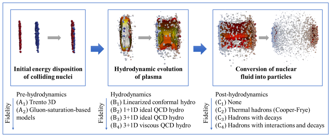
Figure 1: Visualizing the multi-stage multi-fidelity simulator for the quark-gluon plasma.

To address this, we present a new Graphical Multi-fidelity Gaussian process (GMGP) model, which utilizes a directed acyclic graph (DAG) to capture scientific dependencies between simulation models with different fidelities. This DAG structure is elicited via a careful inspection of the scientific models, which we discuss later. The GMGP embeds this DAG within a Gaussian process framework, thus allowing for a more structured and science-driven approach for pooling information from lower-fidelity data for high-fidelity prediction. We show that the GMGP has desirable modeling traits via two Markov properties, and admits an elegant recursive formulation that allows efficient computation of the posterior mean and variance over each depth level of the DAG. We also present a flexible nonlinear extension of the GMGP which leverages deep GPs (Damianou and Lawrence,, 2013). Finally, to maximize predictive power, we propose an efficient experimental design framework for allocating multi-fidelity runs over the DAG given a computational budget. Numerical experiments and an application to heavy-ion collisions demonstrate the improved performance of the GMGP over existing multi-fidelity models.

While the GMGP is motivated from our nuclear physics problem, it has broad applications for other modern scientific problems. Take, e.g., the adhesion of T-cell molecules (Sung et al.,, 2020), which plays an important role in the development of immunotherapy cancer treatments (Harjunpää et al.,, 2019). The adhesion of T-cells can be modeled via two states of T-cell receptor (TCR), a resting state and an upregulated xTCR state, both of which can be modeled via computer simulations. Such simulations, however, can be very time-intensive, and a biologist may choose to run each state at varying fidelity levels, similar to the earlier heavy-ion simulator. Another application is the simulation of cosmological $N$-body problems in astrophysics, where a dark matter fluid is evolved via gravitational force. Here, the fidelity of the simulator can be controlled at different stages (Ho et al.,, 2022), e.g., the number of macro-particles sampled or the resolution of the spatial domain, which again yields a rich multi-stage simulation framework. The GMGP can leverage this multi-stage structure for efficient scientific computing in astrophysics, where multi-fidelity methods have already shown great promise (Ho et al.,, 2022).

This work can also be viewed through the broader lens of science-driven predictive modeling, which aims to embed known scientific principles as prior knowledge for predictive modeling. In recent years, there has been much development on such predictive models for scientific computing, including the integration of scientific information in the form of shape constraints (Golchi et al.,, 2015; Wang and Berger,, 2016), boundary constraints (Ding et al.,, 2019), spectral information (Chen et al.,, 2021), and manifold embeddings (Zhang et al.,, 2021). Here, the GMGP integrates the DAG dependency structure of the multi-fidelity simulators (i.e., the “science”) as prior knowledge within the GP model, which then allows for improved predictive accuracy over existing methods.

We note that the implications of the GMGP extend beyond the multi-fidelity setting into broader data fusion applications where one can elicit a graphical structure connecting data sources. One such application is networked multisensor data fusion (Xia et al.,, 2009), where data are collected over different nodes on a physical sensor network. Such systems are widely used in manufacturing process monitoring and health care problems. A similar problem is distributed data fusion, where multiple agents collectively infer knowledge about a target process by sensing their local environment; this has broad applications in autonomous cars and unmanned aerial vehicles (Campbell and Ahmed,, 2016).

It should also be noted that, for non-GP-based models, there has been some recent work (Gorodetsky et al., 2020a, ; Gorodetsky et al., 2020b, ) which integrates DAG structure. These papers focus on linear subspace (e.g., polynomial-based) models, which are popular surrogate models in the applied mathematics literature. Our model has three notable distinctions. First, the GMGP makes use of GPs rather than linear subspace models, which provides greater flexibility and robustness in model specification (Gramacy,, 2020). Second, by leveraging error bounds for GP interpolation, we introduce a novel design framework for multi-fidelity experiments which maximizes predictive power given a computational budget. Finally, we provide a scalable and probabilistic framework for modeling nonlinear linkages using deep GPs, via recursive computation of the predictive distribution at each depth level of the DAG. We demonstrate this in a suite of numerical experiments and an application.

The paper is organized as follows. Section 2 provides background and motivation. Section 3 presents the GMGP model, its recursive formulation, and extension for nonlinear model dependencies. Section 4 investigates experimental design approaches. Sections 5 and 6 show the effectiveness of the proposed models in a suite of numerical experiments and an application in heavy-ion collisions. Section 7 concludes the paper.

2 Background & Motivation

2.1 Gaussian process modeling

We first provide a brief overview of Gaussian processes (GPs). Let $\boldsymbol{x}\in\Omega\subseteq\mathbb{R}^{d}$ be the input parameters for the computer simulator, and $Z(\boldsymbol{x})$ be its corresponding output. A GP surrogate model places the following prior on the simulation response surface $Z$:

$$Z(\cdot)\sim\mathcal{GP}(\mu(\cdot),k(\cdot,\cdot)).$$

Here, $\mu(\boldsymbol{x})=\mathbb{E}[Z(\boldsymbol{x})]$ is the mean function of the GP, and $k(\boldsymbol{x},\boldsymbol{x}^{\prime})=\text{Cov}[Z(\boldsymbol{x}),Z(\boldsymbol{x}^{\prime})]$ is its covariance function. Without prior knowledge, $\mu(\cdot)$ is typically set as constant, and $k(\cdot,\cdot)$ is chosen as the squared-exponential or Matérn kernel (Gramacy,, 2020). In what follows, we assume the simulators are deterministic (the standard setting for computer experiments), but the proposed models extend analogously for noisy outputs.

Suppose the simulator is run at inputs $\mathcal{D}=\{\boldsymbol{x}_{1},\cdots,\boldsymbol{x}_{n}\}$, yielding outputs $\boldsymbol{z}=\{Z(\boldsymbol{x}_{1}),\cdots,Z(\boldsymbol{x}_{n})\}$. Conditioning on this data, the predictive distribution of $Z$ at a new input point $\boldsymbol{x}$ becomes $[Z(\boldsymbol{x})|\boldsymbol{z},\mathcal{D}]\sim\mathcal{N}(\mu_{n}(\boldsymbol{x}),\sigma^{2}_{n}(\boldsymbol{x}))$, with posterior mean and variance:

$$\begin{split}\mu_{n}(\boldsymbol{x})&=\mu(\boldsymbol{x})+\boldsymbol{k}(\boldsymbol{x},\mathcal{D})^{T}\boldsymbol{K}(\mathcal{D})^{-1}(\boldsymbol{z}-\boldsymbol{\mu}(\mathcal{D})),\\ \sigma^{2}_{n}(\boldsymbol{x})&=k(\boldsymbol{x},\boldsymbol{x})-\boldsymbol{k}(\boldsymbol{x},\mathcal{D})^{T}\boldsymbol{K}(\mathcal{D})^{-1}\boldsymbol{k}(\boldsymbol{x},\mathcal{D}).\end{split}$$ (1)

Here, $\boldsymbol{k}(\boldsymbol{x},\mathcal{D})=[k(\boldsymbol{x},\boldsymbol{x}_{1}),\cdots,k(\boldsymbol{x},\boldsymbol{x}_{n})]$ is the vector of covariances, $\boldsymbol{\mu}(\mathcal{D})=[\mu(\boldsymbol{x}_{1}),\cdots,\allowbreak\mu(\boldsymbol{x}_{n})]$ is the vector of means, and $\boldsymbol{K}(\mathcal{D})$ is the covariance matrix for the training data. Equation (1) captures the key advantages of GP-based emulators: the closed-form posterior mean $\mu_{n}(\boldsymbol{x})$ provides an efficient emulator of the expensive computer simulator, and the closed-form posterior variance $\sigma^{2}_{n}(\boldsymbol{x})$ quantifies its uncertainty.

2.2 The Kennedy-O’Hagan model

A popular model for multi-fidelity emulation is the Kennedy-O’Hagan model (Kennedy and O’Hagan,, 2000), which models a sequence of computer codes with increasing fidelity via a sequence of linear autoregressive GP models. Let $\{\boldsymbol{z}_{1},\boldsymbol{z}_{2},\cdots,\boldsymbol{z}_{T}\}$ denote the data generated by $T$ levels of code sorted in increasing accuracy, where $\boldsymbol{z}_{t}=\{Z_{t}(\boldsymbol{x}^{t}_{i})\}_{i=1}^{n_{t}}$ is the data from the $t$-th code $Z_{t}$. The KO model assumes the multi-fidelity framework:

$$Z_{t}(\boldsymbol{x})=\rho_{t-1}\cdot Z_{t-1}(\boldsymbol{x})+\delta_{t}(\boldsymbol{x}),\quad Z_{t-1}(\boldsymbol{x})\perp\delta_{t}(\boldsymbol{x}),\quad t=2,\cdots,T.$$ (2)

In words, Equation (2) presumes that, prior to data, the response surface $Z_{t}(\boldsymbol{x})$ can be decomposed as the lower-fidelity surface $Z_{t-1}(\boldsymbol{x})$ times a dependency parameter $\rho_{t-1}$, plus some discrepancy function $\delta_{t}(\boldsymbol{x})$ which models the systematic bias between the two computer simulations. For priors, the first (i.e., lowest-fidelity) surface is assigned a GP prior $Z_{1}(\boldsymbol{x})\sim\mathcal{GP}(\boldsymbol{h}_{1}(\boldsymbol{x})^{T}\boldsymbol{\beta}_{1},\sigma_{1}^{2}r_{1}(\boldsymbol{x},\boldsymbol{x}^{\prime}))$, and subsequent discrepancy terms are then assigned independent GP priors $\delta_{t}(\boldsymbol{x})\sim\mathcal{GP}(\boldsymbol{h}_{t}(\boldsymbol{x})^{T}\boldsymbol{\beta}_{t},\sigma_{t}^{2}r_{t}(\boldsymbol{x},\boldsymbol{x}^{\prime}))$. Here, the vectors $\boldsymbol{h}_{1}(\boldsymbol{x}),\cdots,\boldsymbol{h}_{T}(\boldsymbol{x})$ denote pre-defined basis functions which are used for modeling the prior mean of the GPs, and $\boldsymbol{\beta}_{t}$ are their associated coefficients.

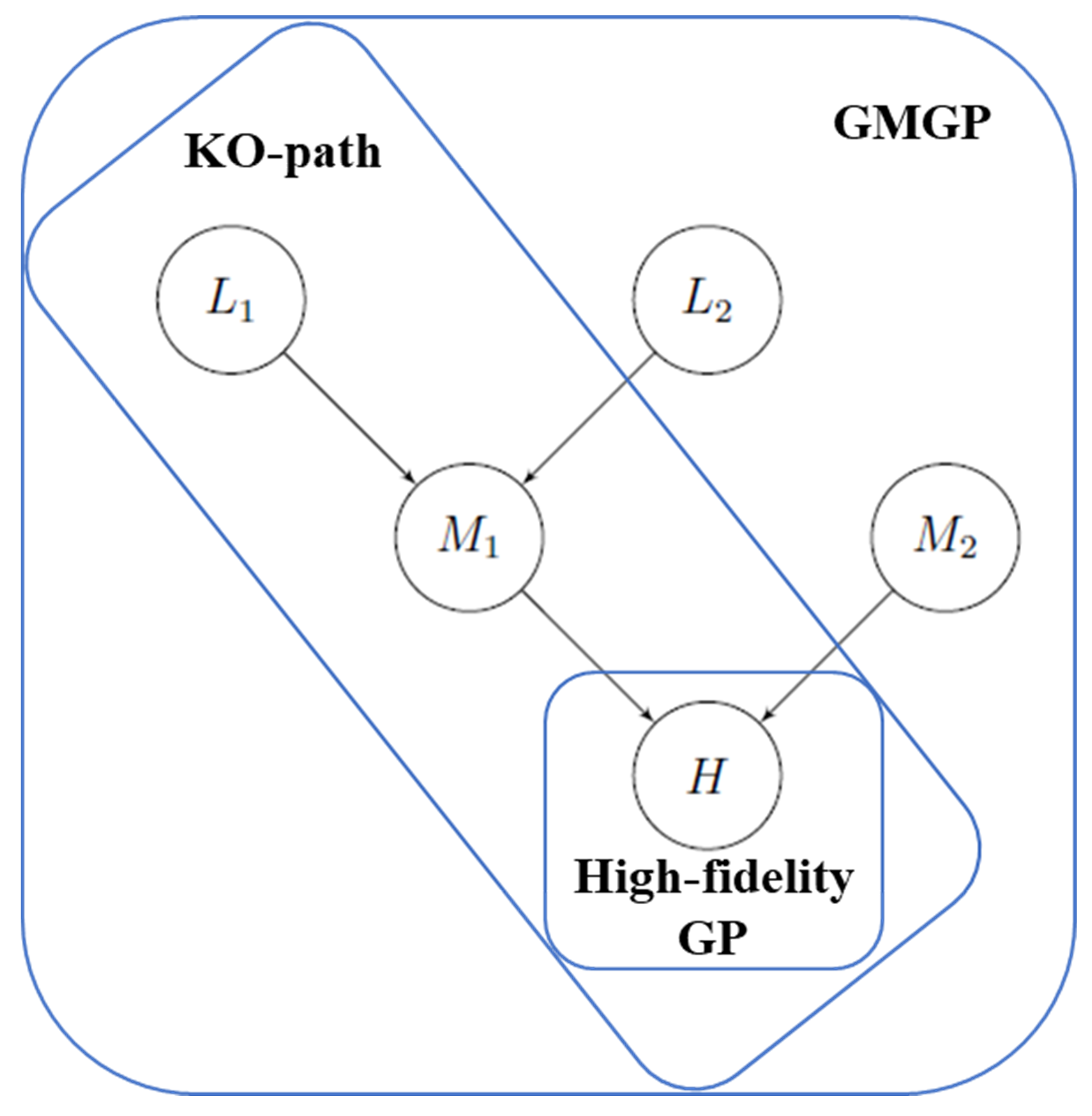
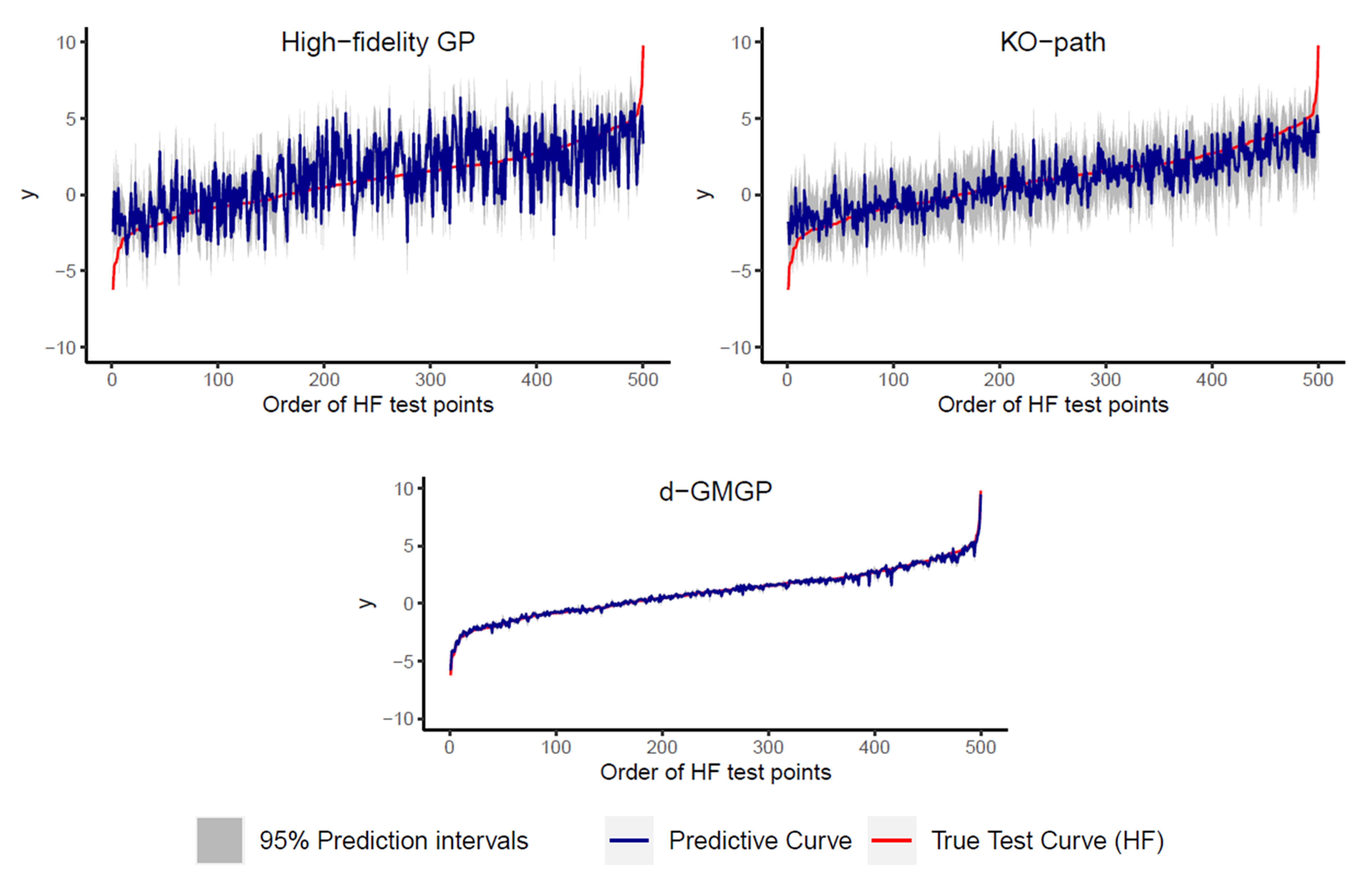
Figure 2: (Left) The five-node DAG used in the 20-dimensional test example. (Right) Predictive performance of the standard high-fidelity GP model (top left), the KO-path model (top right) and the GMGP model (bottom). Red lines mark the high-fidelity (HF) outputs at test inputs, dark blue lines mark the predicted outputs, and gray bands visualize the 95% predictive intervals.

An important development in the KO model is the recursive algorithm proposed by Le Gratiet and Garnier, (2014), which reduces computational complexity of the KO model. The key idea is to substitute the GP prior $Z_{t-1}(\boldsymbol{x})$ in Equation (2) by the posterior distribution ${Z}^{*}_{t-1}(\boldsymbol{x})=[Z_{t-1}(\boldsymbol{x})|\boldsymbol{z}_{1},\cdots,\boldsymbol{z}_{t-1}]$, which can be shown to follow a GP. This recursive formulation expresses the predictive mean and variance at level $t$ as functions of the mean and variance at level $t-1$, which allows for reduced computational cost by avoiding the inversion of large covariance matrices. With a nested structure for design points, Le Gratiet and Garnier, (2014) showed that this recursive formulation yields the same posterior predictive mean and variance as the original KO model, thus justifying the recursive approach. Further discussion will be provided later in Section 3.

One limitation of the KO model (and its extensions) is that it presumes the training data can be ranked from lowest to highest fidelity. Consider a simple example where this is not the case. We take the $d=20$-d test function from Welch et al., (1992) as the high-fidelity simulator, and generate four lower-fidelity representations (details in Section 5). The two medium-fidelity codes ($M_{1}$ and $M_{2}$) are obtained via different simplifications on the high-fidelity code ($H$), and the two low-fidelity codes ($L_{1}$ and $L_{2}$) are obtained by different averaging operations on $M_{1}$. This dependence is captured by the “multi-fidelity DAG” in Fig. 2 (left). Here, the KO model is unable to capture this multi-fidelity structure, since the five simulators cannot be ranked in a sequence. One way to apply the KO model, which we call the “KO-path model”, is to train it on data along the longest path $L_{1}$, $M_{1}$, $H$ (see Fig. 2 (left)); we will explore alternative ways in Section 5.

Fig. 2 (right) shows the performance of the standard GP model trained on 25 design points on $H$, the KO-path model trained on 25 points on $H$, 50 points on $M_{1}$ and 75 points on $L_{1}$, and the proposed GMGP trained on the same data with 50 and 75 additional points on $M_{2}$ and $L_{2}$. Further details on experimental set-up are found in Section 5. Compared to a standard GP, the KO-path model appears to provide slightly improved predictive performance. However, the fitted KO model still exhibits poor predictions over the input space. A natural question is whether we can improve predictive accuracy by integrating the underlying multi-fidelity DAG used for data generation (see Fig. 2 (left)). Fig. 2 (right) answers this in the affirmative: by integrating the multi-fidelity DAG within an appropriate GP model, the proposed GMGP can indeed further improve predictive performance.

3 The Graphical Multi-fidelity Gaussian Process model

3.1 GMGP: model specification

We now present the proposed GMGP model, which generalizes the KO model by embedding the underlying multi-fidelity DAG (capturing scientific dependencies between simulators) as prior information. As noted in the Introduction, our model can be directly applied for broader data fusion settings where data sources can be linked via an underlying graphical structure. For simplicity, we defer such discussion to Section 7 and focus on the multi-fidelity setting from our application.

Let $V$ be the set of nodes representing different simulation codes, and suppose there is a root node $T=|V|\in V$ representing the highest-fidelity simulator. Let $E$ be the set of directed edges connecting different simulation codes, where an edge $(t^{\prime},t)$ is drawn only if node $t$ is a one-step refinement of node $t^{\prime}$, i.e., $t$ is a higher-fidelity refinement of $t^{\prime}$ with no intermediate codes in between. Let $\mathcal{G}=(V,E)$ be the rooted DAG for this multi-fidelity simulation framework. We will discuss later how this “multi-fidelity DAG” can be elicited from a careful inspection of the simulators.

Let $Z_{t}(\boldsymbol{x})$ be the simulation output at input $\boldsymbol{x}$ from code $t$, $t\in V$. The GMGP assumes the following modeling framework:

$$\begin{cases}Z_{t}(\boldsymbol{x})=\sum_{t^{\prime}\in\text{Pa}(t)}\rho_{t^{\prime}}(\boldsymbol{x})Z_{t^{\prime}}(\boldsymbol{x})+\delta_{t}(\boldsymbol{x}),\quad t\in\overline{{V}_{S}},\\ Z_{t^{\prime}}(\boldsymbol{x})\perp\delta_{t}(\boldsymbol{x}),\quad t^{\prime}\in\text{Pa}(t).\end{cases}$$ (3)

Here, $V_{S}\subset V$ consists of all source nodes in $\mathcal{G}$ (i.e., nodes with an in-degree of 0), $\overline{{V}_{S}}=V\setminus V_{S}$ contains the remaining non-source nodes, and $\text{Pa}(t)=\{t^{\prime}\in V:(t^{\prime},t)\in E\}$ consists of all parent nodes of $t\in V$ in the DAG $\mathcal{G}$. Note that source nodes represent simulations with no lower-fidelity representations, and non-source nodes represent simulations with at least one lower-fidelity representation. The function $\rho_{t^{\prime}}(\boldsymbol{x})$ captures dependencies between the output at node $t$ and its lower-fidelity form at node $t^{\prime}$. In the absense of prior information on this dependency linking multi-fidelity models, one can instead adopt $\rho_{t}(\boldsymbol{x})=\rho_{t}$; this is the specification used in later numerical experiments.

We further assign the following GP priors on source nodes:

$$\begin{cases}Z_{t}(\boldsymbol{x})\sim\mathcal{GP}(\boldsymbol{h}_{t}(\boldsymbol{x})^{T}\boldsymbol{\beta}_{t},\sigma_{t}^{2}r_{t}(\boldsymbol{x},\boldsymbol{x^{\prime}})),\quad t\in{V}_{S}\\ Z_{t}(\boldsymbol{x})\perp Z_{t^{\prime}}(\boldsymbol{x}),\quad t,t^{\prime}\in{V}_{S},\quad t\neq t^{\prime}.\end{cases}$$ (4)

Here, $\boldsymbol{h}_{t}(\boldsymbol{x})$ is a vector of basis functions for the response surface mean at node $t$, with $\boldsymbol{\beta}_{t}$ its coefficients. For the discrepancy term $\delta_{t}(\mathbf{x})$, which captures the systematic difference between $Z_{t}(\mathbf{x})$ and its lower-fidelity representations, we assign independent GP priors:

$$\delta_{t}(\boldsymbol{x})\sim\mathcal{GP}(\boldsymbol{h}_{t}(\boldsymbol{x})^{T}\boldsymbol{\beta}_{t},\sigma_{t}^{2}r_{t}(\boldsymbol{x},\boldsymbol{x^{\prime}})),\quad t\in\overline{{V}_{S}}.$$ (5)

Note that this allows for different basis functions at different nodes, which can be specified based on prior information. Without such information, the bases can be set as a constant mean, i.e., $\boldsymbol{h}_{t}(\boldsymbol{x})\equiv 1$, to avoid variance inflation. Here, the kernels at each node employ different length-scale parameters to allow for model flexibility.

While the above specification may seem involved, the intuition is straight-forward. For every non-source node $t\in\overline{{V}_{S}}$, its parent nodes $\text{Pa}(t)$ contain simulations which are lower-fidelity representations of simulation $t$. Equation (3) presumes that, prior to data, $Z_{t}(\boldsymbol{x})$ can be decomposed as the weighted sum of its parent (lower-fidelity) simulations, plus a discrepancy term $\delta_{t}(\boldsymbol{x})$ to model systematic bias. The key novelty over the KO model is that, instead of pooling information in a sequence from lowest to highest fidelity, the GMGP can integrate information over a more general DAG structure, which better captures model dependencies between simulations of complex systems. By leveraging this graphical dependency structure guided by the underlying scientific models, the GMGP can enjoy improved predictive performance over the KO model, as we show later.

The proposition below outlines two appealing modeling properties of the GMGP:

Proposition 1

The GMGP model satisfies the following Markov properties:

1. $Z_{t}(\boldsymbol{x})\perp Z_{t^{\prime}}(\boldsymbol{x})|\{Z_{j}(\boldsymbol{x})\}_{j\in\textup{Pa}(t)},\quad\text{for }t^{\prime}\neq t,\;t^{\prime}\notin\textup{Des}(t),\;t^{\prime}\notin\textup{Pa}(t)$,

2. $Z_{t}(\boldsymbol{x})\perp Z_{t^{\prime}}(\boldsymbol{x}^{\prime})|\{Z_{j}(\boldsymbol{x})\}_{j\in\textup{Pa}(t)},\quad\text{for }t^{\prime}\in\textup{Pa}(t),\;\boldsymbol{x}^{\prime}\neq\boldsymbol{x}$,  if $\mathcal{G}$ is a directed in-tree.

Here, $\textup{Des}(t)$ denotes the set of descendant nodes for $t$, i.e., nodes $t^{\prime}$ for which there exists a path from $t$ to $t^{\prime}$.

The proof is provided in the online supplement, and the formal definition of a directed in-tree is provided and justified in the next section. We note that, without the directed in-tree structure, there may be DAGs $\mathcal{G}$ that violate property (b).

Property $(a)$ states that, for a node $t$ with input $\boldsymbol{x}$, its output $Z_{t}(\boldsymbol{x})$ and the output $Z_{t^{\prime}}(\boldsymbol{x})$ at another node $t^{\prime}$ (where $t^{\prime}$ is a non-descendant, non-parent node of $t$) are conditionally independent, given the simulation output at the parent nodes $\{Z_{j}(\boldsymbol{x})\}_{j\in\text{Pa}(t)}$. In other words, given knowledge of the simulator at its immediate lower-fidelity (i.e., parent) nodes $\text{Pa}(t)$, the output at any simulator $Z_{t^{\prime}}(\boldsymbol{x})$ which is not a higher-fidelity refinement (i.e., not a descendant) of $t$ yields no additional information for predicting the simulator $Z_{t}(\boldsymbol{x})$ at node $t$. This is an intuitive modeling property if the edges in the DAG $\mathcal{G}$ indeed represent model refinements: at fixed input $\boldsymbol{x}$, simulations which are not higher-fidelity refinements of $t$ should yield little (if any) additional information on $t$ given its closest lower-fidelity representations. Property $(a)$ can be viewed as an extension of the conditional independence property for Bayesian network (Stephenson,, 2000). Under a specific form for the multi-fidelity DAG $\mathcal{G}$ (which we justify in the next section), Property $(b)$ states that, conditioning on $\{Z_{j}(\boldsymbol{x})\}_{j\in\text{Pa}(t)}$, the simulation output $Z_{t}(\boldsymbol{x})$ is independent of the parent outputs $Z_{t^{\prime}}(\boldsymbol{x}^{\prime})$ at a different input $\boldsymbol{x}^{\prime}$. In other words, given knowledge of the simulator at its immediate lower-fidelity nodes $\text{Pa}(t)$ with input $\boldsymbol{x}$, the output of such simulators at any other inputs $\boldsymbol{x}^{\prime}$ yields no additional information on predicting the output $Z_{t}(\boldsymbol{x})$ at node $t$. This can be viewed as an extension of the Markov property in O’Hagan, (1998), which was used to justify the KO model.

The modeling framework (3)-(5) can then be used to derive the predictive distribution of the highest-fidelity simulation $Z_{T}(\boldsymbol{x})$. Suppose the model parameters $\Theta=\{\boldsymbol{\beta}_{t}$, $\sigma^{2}_{t}$, $\rho_{t}(\boldsymbol{x})\}_{t=1}^{T}$ are fixed (these can be estimated via maximum likelihood or a fully Bayesian approach; more on this later). Conditional on $\boldsymbol{z}^{(T)}=\{\boldsymbol{z}_{1},\boldsymbol{z}_{2},\cdots,\boldsymbol{z}_{T}\}$, where $\boldsymbol{z}_{t}=\{Z_{t}(\boldsymbol{x}^{t}_{i})\}_{i=1}^{n_{t}}$ are the observed outputs for simulator $t$, the predictive distribution for the highest-fidelity simulation at new input $\boldsymbol{x}$ is given by:

$$[Z_{T}(\boldsymbol{x})|\boldsymbol{z}^{(T)},\Theta]\sim\mathcal{N}(\mu_{Z_{T}}(\boldsymbol{x}),\sigma^{2}_{Z_{T}}(\boldsymbol{x})),$$

where:

$$\begin{split}\mu_{Z_{T}}(\boldsymbol{x})&=\left[\sum_{t^{\prime}\in\text{Pa}(T)}\rho_{t^{\prime}}(\boldsymbol{x})\boldsymbol{h}_{t^{\prime}}(\boldsymbol{x})^{T}\boldsymbol{\beta}_{t^{\prime}}+\boldsymbol{h}_{T}(\boldsymbol{x})^{T}\boldsymbol{\beta}_{T}\right]+\boldsymbol{v}_{T}(\boldsymbol{x})^{T}\boldsymbol{V}_{T}^{-1}(\boldsymbol{z}^{(T)}-H_{T}\boldsymbol{\beta}),\\ \sigma^{2}_{Z_{T}}(\boldsymbol{x})&=v^{2}_{Z_{T}}(\boldsymbol{x})-\boldsymbol{v}_{T}(\boldsymbol{x})^{T}\boldsymbol{V}_{T}^{-1}\boldsymbol{v}_{T}(\boldsymbol{x}).\end{split}$$ (6)

Here, $\boldsymbol{v}_{T}(\boldsymbol{x})=\text{Cov}(Z_{T}(\boldsymbol{x}),\boldsymbol{z}^{(T)})$ is the covariance vector of the new observation $Z_{T}(\boldsymbol{x})$ and data $\boldsymbol{z}^{(T)}$, $\boldsymbol{V}_{T}=\text{Var}(\boldsymbol{z}^{(T)})$ is the covariance matrix of $\boldsymbol{z}^{(T)}$, $v^{2}_{Z_{T}}(\boldsymbol{x})=\text{Var}(Z_{T}(\boldsymbol{x}))$ is the prior variance of $Z_{T}(\boldsymbol{x})$, $H_{T}$ is the matrix of basis functions and $\boldsymbol{\beta}=\{\boldsymbol{\beta}_{1},\cdots,\boldsymbol{\beta}_{T}\}$ are the coefficients such that $H_{T}\boldsymbol{\beta}$ yields the vector of prior means for $\boldsymbol{z}^{(T)}$ from (3).

While Equation (6) provides closed-form expressions for the predictive mean and variance, such expressions can be unwieldy to compute due to the inverse of the large matrix $\boldsymbol{V}_{T}$, which has dimensions $\sum_{t=1}^{T}n_{t}\times\sum_{t=1}^{T}n_{t}$. Motivated by Le Gratiet and Garnier, (2014), we consider below a recursive formulation for the GMGP that performs model training at each depth level of the DAG, thus enabling scalable predictions.

3.2 r-GMGP: recursive formulation

The key idea for the r-GMGP is to recursively perform model training and prediction at each depth level of $\mathcal{G}$, beginning with source (i.e., depth 0) nodes, then continuing for higher depth nodes until the highest-fidelity node is reached. This is facilitated by the following recursive computation of the predictive distribution, which we later show yields the desired predictive mean and variance from the GMGP (3) under certain conditions:

$$\begin{cases}Z_{t}(\boldsymbol{x})=\sum_{t^{\prime}\in\text{Pa}(t)}\rho_{t^{\prime}}(\boldsymbol{x})Z^{*}_{t^{\prime}}(\boldsymbol{x})+\delta_{t}(\boldsymbol{x}),\quad t\in\overline{{V}_{S}},\\ Z^{*}_{t^{\prime}}(\boldsymbol{x})\perp\delta_{t}(\boldsymbol{x}),\quad t^{\prime}\in\text{Pa}(t).\end{cases}$$ (7)

Here, $Z^{*}_{t^{\prime}}(\cdot)=[Z_{t^{\prime}}(\cdot)|\{\boldsymbol{z}_{m}\}_{m\in\text{Anc}(t^{\prime})},\boldsymbol{z}_{t^{\prime}},{\color[rgb]{0,0,0}{\Theta_{t^{\prime}}}}]$ is the posterior distribution at node $t^{\prime}$, conditional on data from both $t^{\prime}$ and its ancestor nodes $\text{Anc}(t^{\prime})$, i.e., nodes $u$ where there exists a path from $u$ to $t^{\prime}$. The exact expression for $Z^{*}_{t^{\prime}}(\cdot)$ is given in Equation (8) below, with $T$ replaced by the current node. The same GP priors (5) are assigned for the discrepancy terms $\delta_{t}(\boldsymbol{x})$. The key difference between the recursive GMGP (r-GMGP) formulation (7) and the GMGP (3) is that, in place of $Z_{t^{\prime}}(\boldsymbol{x})$ (the prior of the parent simulation) for the GMGP, the r-GMGP uses $Z^{*}_{t^{\prime}}(\boldsymbol{x})$, the posterior of the parent simulation given data.

Under (7), the posterior distribution of the highest-fidelity simulation $Z_{T}$ becomes:

$$[Z_{T}(\boldsymbol{x})|\boldsymbol{z}^{(T)},\Theta]\sim\mathcal{N}(m_{Z_{T}}(\boldsymbol{x}),s^{2}_{Z_{T}}(\boldsymbol{x})),$$

with the posterior mean $m_{Z_{T}}(\boldsymbol{x})$ and variance $s^{2}_{Z_{T}}(\boldsymbol{x})$:

$$\small\begin{split}m_{Z_{T}}(\boldsymbol{x})&=\sum_{t^{\prime}\in\text{Pa}(T)}\rho_{t^{\prime}}(\boldsymbol{x})m_{Z_{t^{\prime}}}(\boldsymbol{x})+\boldsymbol{h}_{T}(\boldsymbol{x})^{T}\boldsymbol{\beta}_{T}\\ &\quad\quad\quad+\boldsymbol{r}_{T}(\boldsymbol{x},\mathcal{D}_{T})^{T}\boldsymbol{R}_{T}(\mathcal{D}_{T})^{-1}\left[\boldsymbol{z}_{T}-\sum_{t^{\prime}\in\text{Pa}(T)}\boldsymbol{\rho}_{t^{\prime}}(\mathcal{D}_{T})\odot\boldsymbol{z}_{t^{\prime}}(\mathcal{D}_{T})-\boldsymbol{h}_{T}(\mathcal{D}_{T})^{T}\boldsymbol{\beta}_{T}\right],\\ s^{2}_{Z_{T}}(\boldsymbol{x})&=\sum_{t^{\prime}\in\text{Pa}(T)}\rho^{2}_{t^{\prime}}(\boldsymbol{x})s^{2}_{Z_{t^{\prime}}}(\boldsymbol{x})+\sigma^{2}_{T}\left[1-\boldsymbol{r}_{T}(\boldsymbol{x},\mathcal{D}_{T})^{T}\boldsymbol{R}_{T}(\mathcal{D}_{T})^{-1}\boldsymbol{r}_{T}(\boldsymbol{x},\mathcal{D}_{T})\right].\end{split}$$ (8)

Here, $\odot$ denotes the Hadamard (entrywise) product, $\mathcal{D}_{T}=\{\boldsymbol{x}_{i}^{T}\}_{i=1}^{n_{T}}$ is the set of design points at node $T$, $\boldsymbol{r}_{T}(\boldsymbol{x},\mathcal{D}_{T})$ is the correlation vector between $Z_{T}(\boldsymbol{x})$ and $\boldsymbol{z}_{T}$, and $\boldsymbol{R}_{T}(\mathcal{D}_{T})$ is the correlation matrix of $\boldsymbol{z}_{T}$. Equation (8) provides closed-form expressions for the predictive distribution of the highest-fidelity simulation $T$, which depend on only terms related to the current node $T$ and its parent nodes $\text{Pa}(T)$. Indeed, Equation (8) holds for all non-source nodes $t\in\overline{V_{S}}$, with closed-form expressions depending on only node $t$ and its parent nodes $\text{Pa}(t)$. Thus, the desired predictive distribution $[Z_{t}(\boldsymbol{x})|\boldsymbol{z}^{(T)},\Theta]$ can be efficiently evaluated, by recursively computing the posterior mean and variance using (8) at each depth level of $\mathcal{G}$, starting from its leaf nodes to its root. We show later that the predictive equations (8) for r-GMGP are precisely the desired predictive equations (6) for the GMGP model under certain conditions.

This recursive approach can yield significant computational savings over a naive evaluation of the original predictive equations (6), since it breaks up the inversion of the large covariance matrix $\boldsymbol{V}_{T}$ into inversions of smaller matrices $\boldsymbol{R}_{t}(\mathcal{D}_{t})$ at each depth level of $\mathcal{G}$. More precisely, with $n_{t}$ denoting the sample size at node $t\in V$, this reduces the computational cost of $\mathcal{O}((\sum_{t\in V}n_{t})^{3})$ for the original predictive equations (6) to a cost of $\mathcal{O}(\sum_{t\in V}n_{t}^{3})$ for the recursive approach in (8). Furthermore, if the inverse at each level of $\mathcal{G}$ can be performed simultaneously via distributed computing, this computational cost can be further reduced to $\mathcal{O}(D\max_{t}(n_{t})^{3})$, where $D\leq T$ is the depth of the rooted graph $\mathcal{G}$. When the sample sizes are moderately large at most nodes (which is typically the case for low-fidelity simulations), this recursive computation of the posterior mean and variance at each depth level can yield large computational savings.

We now return to the important question of whether the r-GMGP predictive equations (8) are indeed the same as the desired predictive equations (6) for GMGP. To show this equivalence, we require a specific structure of the multi-fidelity DAG $\mathcal{G}$. Suppose $\mathcal{G}$ is a directed in-tree (Mehlhorn and Sanders,, 2008), defined as a rooted tree for which, at any node $t\in V$, there is exactly one path going from node $t$ to the root node $T$ (representing the highest-fidelity simulator $Z_{T}$). In-trees are also known as anti-arborescence trees (Korte and Vygen,, 2011) in graph theory. Fig. 3 shows several examples of directed in-trees.

Figure 3: Examples of in-trees, with $Z_{T}$ denoting the highest-fidelity simulator at the root.

Under such an assumption on $\mathcal{G}$, the following proposition shows that the r-GMGP indeed yields the desired posterior predictive mean and variance for the highest-fidelity simulation $Z_{T}$ for the GMGP model:

Proposition 2

Suppose the rooted multi-fidelity DAG $\mathcal{G}=(V,E)$ is an in-tree. Further suppose (i) the observations are noise-free, and (ii) the design points are nested over $\mathcal{G}$, such that for any node $t\in V$, its design set $\mathcal{D}_{t}$ is a subset of the designs at all parent nodes $\mathcal{D}_{t^{\prime}},\ t^{\prime}\in\textup{Pa}(t)$. Then, conditional on the parameters $\Theta=\{\boldsymbol{\beta}_{t}$, $\sigma^{2}_{t}$, $\rho_{t}(\boldsymbol{x})\}_{t=1}^{T}$ of both models, the posterior predictive mean and variance from GMGP and r-GMGP are the same, i.e., $\mu_{Z_{T}}(\boldsymbol{x})=m_{Z_{T}}(\boldsymbol{x})$ and $\sigma^{2}_{Z_{T}}(\boldsymbol{x})=s^{2}_{Z_{T}}(\boldsymbol{x})$, where $\mu_{Z_{T}}(\boldsymbol{x})$ and $\sigma^{2}_{Z_{T}}(\boldsymbol{x})$ are the GMGP posterior mean and variance in (6), and $m_{Z_{T}}(\boldsymbol{x})$ and $s^{2}_{Z_{T}}(\boldsymbol{x})$ are the r-GMGP posterior mean and variance in (8).

The proof (by induction) is provided in the online supplement. This proposition shows that the recursive GMGP formulation indeed yields the same predictive mean and variance as the GMGP model when the multi-fidelity graph $\mathcal{G}$ forms an in-tree, thus justifying the computational savings from r-GMGP. The assumption of $\mathcal{G}$ being an in-tree implies that, for any simulator (i.e., node), there exists exactly one path in the employed simulation framework along which this model can be refined to the highest-fidelity simulator (i.e., root node). For example, the three heavy-ion collision models in the Introduction form a 3-node in-tree (see Fig. 5 (left)). In practice, such a property can often be satisfied via a careful choice of lower-fidelity simulators to run for training the multi-fidelity emulator. In cases where the simulators cannot be selected and do not form an in-tree, the original GMGP equations (6) may be used for prediction, albeit at higher costs from larger matrix inversions.

For inference on model parameters, we employ a straight-forward extension of the maximum likelihood approach in Le Gratiet and Garnier, (2014), which accounts for uncertainties in regression and dependency parameters within a universal co-kriging framework. Details can be found in Le Gratiet and Garnier, (2014). In particular, our implementation of r-GMGP is built upon the R package MuFiCokriging (Le Gratiet,, 2012) for this paper, which is available on CRAN. If fully Bayesian inference is desired on such parameters, one can adapt the Monte Carlo approach in Konomi and Karagiannis, (2021).

Finally, we note that while the above formulation presumes independence over source nodes, there may be situations where prior information suggests some correlation may be preferable between these nodes. In such cases, one may adopt correlated GP priors over source nodes, then use the original GMGP without recursive updates.

3.3 d-GMGP: nonlinear extension

One potential limitation of the GMGP is that it presumes linear dependencies between the simulation codes over the DAG. Given enough training data, it may be preferable to consider a more sophisticated emulator model that accounts for nonlinear dependencies between nodes on the multi-fidelity DAG. There are multiple ways for modeling this, including the deep GP approach in Perdikaris et al., (2017) and the binary tree partition method in Konomi and Karagiannis, (2021). Below, we adapt the deep GP approach for two reasons: (i) the output observables in our high-energy physics application are known to be quite smooth (Everett et al., 2021b, ), thus the smoother deep GP approach is preferable to binary tree partitions; (ii) our extension avoids the need for MCMC sampling in approximating the predictive distribution.

Similar to before, let us assume the multi-fidelity DAG $\mathcal{G}$ is a directed in-tree, with design points nested over $\mathcal{G}$. The d-GMGP model at non-source nodes is formulated as:

$$\begin{cases}Z_{t}(\boldsymbol{x})=f_{t}(\{Z_{t^{\prime}}(\boldsymbol{x}):t^{\prime}\in\text{Pa}(t)\}\cup\boldsymbol{x})+\delta_{t}(\boldsymbol{x}),\quad t\in\overline{{V}_{S}},\\ f_{t}(\cdot)\perp\delta_{t}(\cdot).\end{cases}$$ (9)

Here, we again assign independent GP priors for the discrepancies $\delta_{t}(\boldsymbol{x})\sim\mathcal{GP}(0,\sigma_{t}^{2}r_{t}(\boldsymbol{x},\boldsymbol{x}^{\prime}))$, with similar independent GP priors on source nodes:

$$\begin{cases}Z_{t}(\boldsymbol{x})\sim\mathcal{GP}(0,\sigma_{t}^{2}r_{t}(\boldsymbol{x},\boldsymbol{x^{\prime}})),\quad t\in{V}_{S},\\ Z_{t}(\boldsymbol{x})\perp Z_{t^{\prime}}(\boldsymbol{x}),\quad t,t^{\prime}\in{V}_{S},\quad t\neq t^{\prime}.\end{cases}$$ (10)

The key difference between this new model and the GMGP model (3) is how the lower-fidelity (parent) nodes are integrated for higher-fidelity models. Instead of a weighted sum of the parent codes $\sum_{t^{\prime}\in\text{Pa}(t)}\rho_{t^{\prime}}(\boldsymbol{x})Z_{t^{\prime}}(\boldsymbol{x})$, the d-GMGP model allows for a more general nonlinear transformation $f_{t}(\cdot)$ of the parent codes $\{Z_{t}(\boldsymbol{x}):t\in\text{Pa}(t)\}$ as well as the control parameters $\boldsymbol{x}$.

Since the transformation $f_{t}$ is unknown in practice, one approach is to assign to it an independent zero-mean GP prior. We can combine the GP priors on $f_{t}$ and $\delta_{t}$ with Equation (9) to obtain the general specification for $Z_{t}(\boldsymbol{x})$ for non-source node $t\in\overline{V_{S}}$:

$$Z_{t}(\boldsymbol{x})=g_{t}(\{Z_{t^{\prime}}(\boldsymbol{x}):t^{\prime}\in\text{Pa}(t)\}\cup\boldsymbol{x})\sim\mathcal{GP}(0,K_{t}([\boldsymbol{x},\boldsymbol{z}],[\boldsymbol{x}^{\prime},\boldsymbol{z}^{\prime}])),\quad t\in\overline{V_{S}},$$ (11)

where $\boldsymbol{z}=\{Z_{t^{\prime}}(\boldsymbol{x})\}_{t^{\prime}\in\text{Pa}(t)}$ and $\boldsymbol{z}^{\prime}=\{Z_{t^{\prime}}(\boldsymbol{x}^{\prime})\}_{t^{\prime}\in\text{Pa}(t)}$. Note that the kernel $K_{t}$ involves both the control parameters $\boldsymbol{x}$ and the simulation outputs $Z_{t^{\prime}}(\boldsymbol{x})$ from lower-fidelity (parent) nodes $t^{\prime}\in\text{Pa}(t)$. Viewed this way, the proposed d-GMGP model can be seen as an extension of the deep GP model (see, e.g., Damianou and Lawrence,, 2013), where the GP outputs at each node are linked by the multi-fidelity DAG elicted from model dependencies (i.e., the “science”). Compared to a full-blown deep GP model, which typically requires the estimation of thousands of variational parameters, the d-GMGP model (11) with the kernel choice below requires much fewer parameters for estimation, all the while providing the desired nonlinear dependency over the graph.

For the kernel $K_{t}$ in (11), one specification we found quite effective is the following:

$$K_{t}([\boldsymbol{x},\boldsymbol{z}],[\boldsymbol{x}^{\prime},\boldsymbol{z}^{\prime}])=K_{\rm SE,{\color[rgb]{0,0,0}}}(\boldsymbol{x},\boldsymbol{x}^{\prime})\left[K_{\rm LIN}(\boldsymbol{z},\boldsymbol{z}^{\prime})+K_{\rm SE}(\boldsymbol{z},\boldsymbol{z}^{\prime})\right]+K_{\rm SE,{\color[rgb]{0,0,0}}}(\boldsymbol{x},\boldsymbol{x}^{\prime}),\quad t\in\overline{V_{S}}.$$ (12)

Here, $K_{\rm LIN}(\boldsymbol{z},\boldsymbol{z}^{\prime})=\sigma^{2}\boldsymbol{z}^{T}\boldsymbol{z}^{\prime}$ is a linear kernel, $\sigma^{2}$ is a variance parameter, and $K_{\rm SE}(\boldsymbol{z},\boldsymbol{z}^{\prime})$, $K_{\rm{SE},\rho}(\boldsymbol{x},\boldsymbol{x}^{\prime})$ and $K_{\rm{SE},\delta}(\boldsymbol{x},\boldsymbol{x}^{\prime})$ are separate anisotropic squared-exponential kernels. This is motivated by the kernel choice for the deep multi-fidelity GP models in Perdikaris et al., (2017) and Cutajar et al., (2019). The intuition behind (12) is that it captures both linear and nonlinear dependencies between outputs, as well as correlations between input parameters. When $K_{\rm SE}(\boldsymbol{z},\boldsymbol{z}^{\prime})=0$, this kernel reduces to a form similar to the r-GMGP, with a probabilistic and non-parametric form for $\rho(\boldsymbol{x})$. In total, the d-GMGP with kernel (12) requires $(1+d)|V_{S}|+\sum_{t\in\overline{V_{S}}}(4+2d+|\text{Pa}(t)|)$ hyperparameters to estimate (via maximum likelihood), which is much fewer than that needed for a full-scale deep GP; this is primarily due to the above recursive formulation. Such a deep model, however, requires the estimation of more parameters compared to the r-GMGP and thus requires more computation for inference and prediction; it should therefore be used only when one has prior information on nonlinear dependencies. When model outputs are known to be highly non-stationary and/or discontinuous, the binary tree partition approach in Konomi and Karagiannis, (2021) may offer an appealing alternative for computational efficiency.

As before, a recursive formulation can be adopted for efficient fitting of the d-GMGP. The idea is again to recursively perform model training and prediction at each depth level of $\mathcal{G}$. This is achieved by replacing the GP priors $Z_{t^{\prime}}(\cdot)$, $t^{\prime}\in\text{Pa}(t)$ in Equation (9) by the GP posteriors $Z^{*}_{t^{\prime}}(\cdot)=[Z_{t^{\prime}}(\cdot)|\{\boldsymbol{z}_{m}\}_{m\in\text{Anc}(t^{\prime})},\boldsymbol{z}_{t^{\prime}},{\color[rgb]{0,0,0}{\Theta_{t^{\prime}}}}]$, $t^{\prime}\in\text{Pa}(t)$. The desired posterior on the highest-fidelity node $Z_{T}(\cdot)$ can then be computed recursively at each depth level of $\mathcal{G}$, starting from its leaf nodes to its root, as was done for the r-GMGP. Unlike the r-GMGP, however, the predictive distribution for the highest-fidelity node $Z_{T}(\cdot)$ is no longer Gaussian. This recursive formulation allows for efficient approximation of the desired predictive distribution, by propagating the posterior uncertainty at each level using Monte Carlo. Specifically, the posterior distribution at a non-source node $t$ can be evaluated by:

$$[Z_{t}^{*}(\boldsymbol{x})]=\int[Z_{t}(\boldsymbol{x})|\boldsymbol{z}_{t},\boldsymbol{z^{*}}]\prod_{t^{\prime}\in\text{Pa}(t)}[Z_{t^{\prime}}^{*}(\boldsymbol{x})]\;d\boldsymbol{z}^{*}.$$ (13)

Here, $\boldsymbol{z}_{t}$ are the observed data on node $t$, and $\boldsymbol{z^{*}}=\{Z^{*}_{t^{\prime}}(\boldsymbol{x})\}_{t^{\prime}\in\text{Pa}(t)}$ are the (unknown) outputs on parent nodes at parameters $\boldsymbol{x}$. This can be estimated via Monte Carlo integration on the posterior of parent node outputs $[Z_{t^{\prime}}^{*}(\boldsymbol{x})]$, $t^{\prime}\in\text{Pa}(t)$. This procedure can then be repeated recursively at each depth level of $\mathcal{G}$ to provide efficient computation of the predictive distribution for the highest-fidelity node $Z_{T}(\cdot)$. Compared to full-scale deep GP model, this recursive approach provides a scalable way for propagating predictions and uncertainties to the root node, without the need for complex variational approximations. The full algorithm for d-GMGP prediction is provided in the online supplement.

For the d-GMGP, the computational cost for hyperparameter estimation using maximum likelihood is $\mathcal{O}(\sum_{t\in V}n_{t}^{3})$ per objective evaluation, which greatly speeds up the $\mathcal{O}((\sum_{t\in V}n_{t})^{3})$ cost for standard GP via its recursive formulation. Its prediction then requires sampling from the posterior distribution of each parent node model, then propagating these as inputs of each child node until we reach the root of the tree. Here, the posterior samples needed to achieve a desired accuracy for highest-fidelity prediction can grow exponentially with both the input dimensions and the size of the tree. One solution (which we adopt) is to employ a Gaussian approximation of the posterior predictive distribution at each node, then recursively compute the posterior means and variances over the nodes in DAG $\mathcal{G}$. The latter step can be performed via the closed-form expressions in Girard et al., (2002), and further details of this can be found in Perdikaris et al., (2017).

In choosing between the original GMGP model (which models linear dependencies) or the above d-GMGP model, we have found that with careful elicitation from scientists, there is often prior knowledge on scientific model dependencies which can help guide this choice. For example, in computational fluid dynamics (see, e.g., Wang,, 2016), the dependencies between the high-fidelity direct numerical simulation (Pope,, 2000) and the lower-fidelity Reynolds-averaged Navier Stokes simulation (Catalano and Amato,, 2003) is known to be highly nonlinear, and captures complex eddies and vortices in turbulent fluid flow. For this case, the d-GMGP should be thus used instead of the original GMGP model. In the absence of such prior information, one can make use of standard model selection techniques (e.g., AIC or BIC) to select the better predictive model from data.

4 Experimental Design

Given that the motivation behind the GMGP model is to maximize predictive performance given a computational budget, its experimental design is of crucial importance. This procedure can be split into two steps: (i) the design of training set $\mathcal{D}_{t}$ at each node $t\in V$ given fixed sample sizes $n_{t}=|\mathcal{D}_{t}|$, and (ii) the allocation of sample sizes $n_{t}$ at each node $t\in V$ given a fixed computational budget. For simplicity, we investigate this for the GMGP model, but such designs can naturally be adapted for the more complex d-GMGP model. As before, we assume the underlying DAG is an in-tree.

4.1 Design given fixed sample sizes

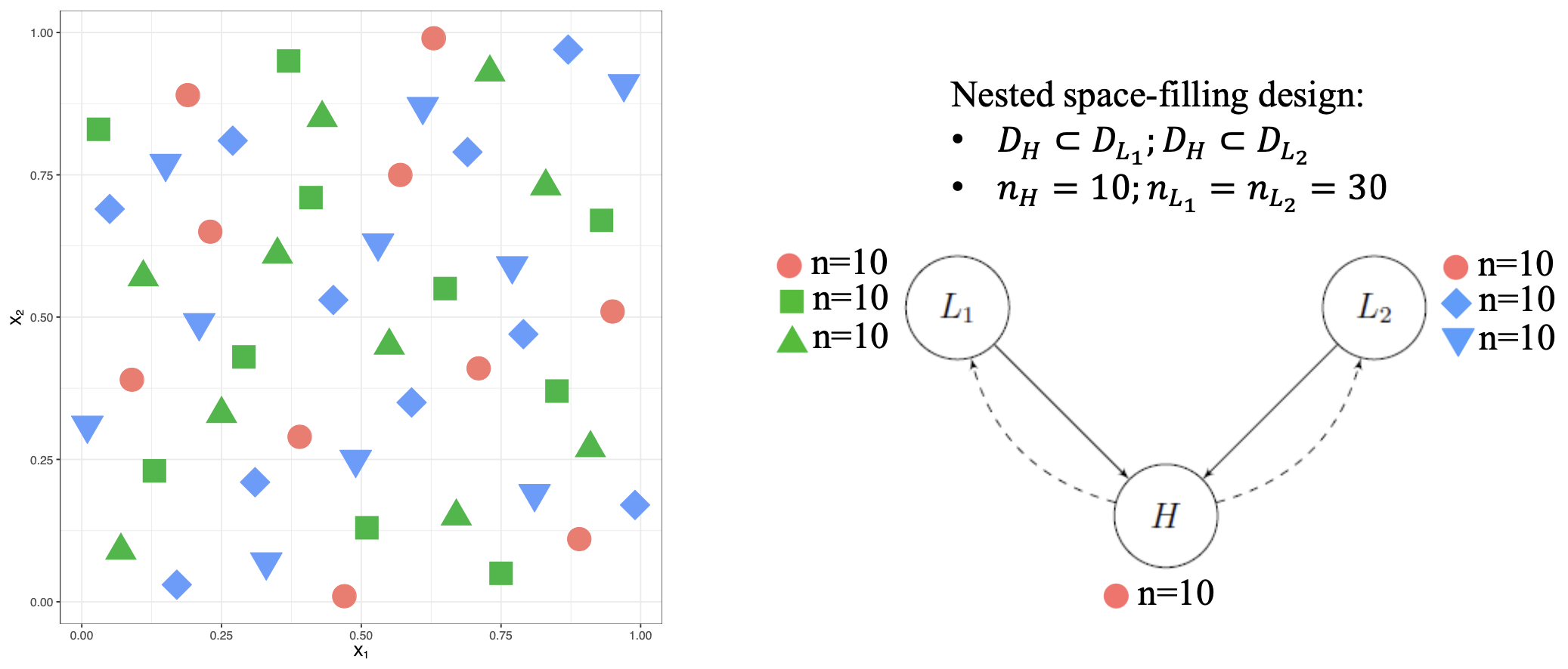
Figure 4: Visualizing our nested BFS design on a $2$-d space. (Left) The base maximin SLHD design with 5 slices and 10 design points per slice. (Right) BFS allocation of the SLHD design over a three-node DAG. The first slice (red) is allocated to all three nodes, then subsequent slices (green and blue) are used on the lower-fidelity nodes $L_{1}$ and $L_{2}$.

Consider first step (i). From Proposition 2, an appealing design property is the nested nature of design points over the graph $\mathcal{G}$, i.e., for any node $t\in V$, the design set $\mathcal{D}_{t}$ is a subset of the designs $\mathcal{D}_{t^{\prime}}$ at any parent node $t^{\prime}\in\text{Pa}(t)$. For GP modeling, the space-filling property of design points (Santner et al.,, 2019) – its uniformity over the prediction space – is also known to be crucial for improving predictive performance. Different notions of space-fillingness have been explored in the literature, including maximin (Johnson et al.,, 1990; Morris and Mitchell,, 1995) and minimax designs (Johnson et al.,, 1990; Mak and Joseph,, 2018). We will incorporate these two properties in the design procedure below.

Algorithm 1 Nested BFS Design

Input: DAG with $T=|V|$ nodes; desired sample sizes $\{n_{t}:\ t\in V\}$. Note that all $n_{t}$’s should be multiples of $n_{T}$.
Output: Design set $\mathcal{D}_{t}$ for each node $t\in V$.

1:Generate a maximin SLHD design (Ba et al.,, 2015) with $M=\sum_{t=1}^{T}{n_{t}}/{n_{T}}$ slices, with each slice containing $n_{T}$ design points.

2:Assign the design points in slices $\{\sum_{j=1}^{t-1}{n_{j}}/{n_{T}}+1,\cdots,\sum_{j=1}^{t}{n_{j}}/{n_{T}}\}$ (denoted as $S_{t}$) to node $t$, $t=1,\cdots,T$.

3:For each node $t$, set $\mathcal{D}_{t}=S_{t}\cup\ \left\{\cup_{t^{\prime}\in\text{Des}(t)}S_{t^{\prime}}\right\}$ for $t=1,\cdots,T$.

Given sample sizes $n_{1},\cdots,n_{T}$, we propose a nested experimental design over the DAG $\mathcal{G}$. We make use of the maximin sliced Latin hypercube design (maximin SLHD, Ba et al.,, 2015; see also Qian,, 2012), which provides design points in equal slices (or batches), such that the design points within each slice are space-filling, and the design points between slices are also well spaced-out. Fig. 4 (left) shows an SLHD in $d=2$ dimensions. With this SLHD in hand, we then employ a bottom-up approach to allocate design points over $\mathcal{G}$. We first allocate one slice in the SLHD for the highest-fidelity simulator $T$ (i.e., the root node at the bottom of $\mathcal{G}$), then use the remaining slices to fill out design points on subsequent nodes in a breadth-first-traversal (BFS) of $\mathcal{G}$. For the latter step, the design points at each node $t\in V$ are obtained by concatenating the current SLHD slice(s) with design points on its descendant nodes $\text{Des}(t)$; this ensures the design is nested over the DAG $\mathcal{G}$. Fig. 4 (right) visualizes this nested BFS design procedure. Intuitively, the use of maximin SLHDs allows one to “maximize” the information obtained over different nodes for predicting the high-fidelity response surface (we provide a more formal discussion of this in the next subsection). Algorithm 1 provides the detailed steps.

To implement this nested BFS design, however, there are certain conditions which need to hold for the sample sizes $n_{1},\cdots,n_{T}$. The first condition is that $n_{t^{\prime}}\geq n_{t}$ if edge $(t^{\prime},t)\in E$, i.e., a lower-fidelity node should always have as many sample points as its higher-fidelity counterpart. This is reasonable in practice, since lower-fidelity simulations are by nature cheaper than higher-fidelity ones. The second condition is that the sample size $n_{t}$ at any node $t$ should be a multiple of the sample size $n_{T}$ at the root (highest-fidelity) node. This allows us to evenly allocate slices of design points over each node, thus maximizing the value from the sliced LHD structure. As we show later, this can be satisfied by simply rounding off the sample sizes optimized in the following subsection.

4.2 Sample size allocation given fixed computational budget

Consider next step (ii), the allocation of sample sizes $n_{t}$ given a fixed budget $C$. Let $C_{t}$ be the cost of performing a single run at simulation node $t\in V$, and let $n_{t}$ be the allocated sample size at node $t$. The budget constraint can thus be written as $\sum_{t\in V}C_{t}n_{t}\leq C$.

We now derive a design criterion to minimize under this constraint for the sample sizes $n_{1},\cdots,n_{T}$. This follows from the proposition below (adapted from Wu and Schaback,, 1993), which provides an upper bound on prediction error from the GMGP model. In what follows, we denote the response surface at source nodes by $\delta_{t}(\boldsymbol{x})$, $t\in V_{S}$.

Proposition 3

Suppose the highest-fidelity simulation $Z_{T}(\boldsymbol{x})$ follows the recursive model (7). Further suppose that: (i) the parameter space $\Omega$ is bounded and convex, and (ii) the discrepancy term $\delta_{t}(\boldsymbol{x})$ is in the native space $N_{r_{t}}(\Omega)$ equipped with norm $||\cdot||_{N_{r_{t}}(\Omega)}$, where $r_{t}$ (the correlation function in (5)) is the Matérn kernel with smoothness parameter $\nu$. Then, using the posterior mean $m_{Z_{T}}(\boldsymbol{x})$ in (8), the prediction error can be upper bounded by:

$$|Z_{T}(\boldsymbol{x})-m_{Z_{T}}(\boldsymbol{x})| \leq\sum_{t=1}^{T}\left(\prod_{t^{\prime}\in\mathrm{Des}(t)\cup\{t\}\setminus\{T\}}|\rho_{t^{\prime}}(\boldsymbol{{x})}|\right)c_{r_{t}}h_{\mathcal{D}_{t}}^{\nu}||\delta_{t}(\boldsymbol{x})||_{N_{r_{t}}(\Omega)}.$$ (14)

Here, $h_{\mathcal{D}_{t}}=\max_{\boldsymbol{x}\in\Omega}\min_{i=1,\cdots,n_{t}}\|\boldsymbol{x}-\boldsymbol{x}_{i}^{t}\|_{2}$ is the fill distance of design $\mathcal{D}_{t}$, and $c_{r_{t}}$ is a constant depending on the length-scale parameters of $r_{t}$.

Our goal is to find an optimal allocation of sample sizes $n_{1},\cdots,n_{T}$ to minimize the error bound on the right side of (14), which in turn reduces the GMGP prediction error.

However, prior to data, we do not know what $\rho_{t}(\boldsymbol{x})$ and $||\delta_{t}(\boldsymbol{x})||_{N_{r_{t}}(\Omega)}$ are, and thus require further assumptions to evaluate the desired error bound. Suppose we make the simplifying assumptions that, prior to data, the dependency functions are constant over all nodes, i.e., $|\rho_{t}(\boldsymbol{x})|=\rho$, and that the native norm of the discrepancies are constant, i.e., $||\delta_{t}(\boldsymbol{x})||_{N_{r_{t}}(\Omega)}=\Delta$. Then, ignoring proportionality constants, the bound in (14) reduces to $\sum_{t=1}^{T}\rho^{|\text{Des}(t)|}h_{\mathcal{D}_{t}}^{\nu}$. Additionally, if the design points $\mathcal{D}_{t}$ at each node $t\in V$ are distributed in a manner which minimizes the fill distance asymptotically (this property is known as low-dispersion; see, e.g., Fang and Wang,, 1993), then it is known that $h_{\mathcal{D}_{t}}=\mathcal{O}(n_{t}^{-1/d})$ (Wendland,, 2004). This low-dispersion property is satisfied by most space-filling criteria (Pronzato,, 2017). With this, the bound further simplifies to:

$$\sum_{t=1}^{T}\rho^{|\text{Des}(t)|}{n_{t}}^{-\nu/d}=:\Phi_{\rho}(n_{1},\cdots,n_{T}),$$ (15)

where $|\text{Des}(t)|$ is the number of descendant nodes on $t$. Consider now the minimization of the simplified bound $\Phi_{\rho}(n_{1},\cdots,n_{T})$ given the budget constraint, i.e.:

$$\min_{n_{1},\cdots,n_{T}}\Phi_{\rho}(n_{1},\cdots,n_{T})\quad\text{s.t.}\quad\sum_{t\in V}C_{t}n_{t}\leq C.$$ (16)

Using the method of Lagrange multipliers with Karush-Kuhn-Tucker conditions (Nocedal and Wright,, 2006), the optimal sample sizes can then be solved in closed-form as:

$$n_{t}\propto\left(\frac{\rho^{|\text{Des}(t)|}}{C_{t}}\right)^{d/(d+\nu)},\quad\sum_{t\in V}C_{t}n_{t}=C.$$ (17)

Equation (17) provides a nice closed-form expression for sample size allocation over the multi-fidelity graph $\mathcal{G}$, where each node $t$ has a different cost $C_{t}$ per run. This yields two useful interpretations. First, nodes with higher costs per run are assigned smaller sample sizes by (17), which is intuitive since such experiments demand more computational resources. Second, assuming $\rho\in(0,1)$, nodes with a greater number of descendant nodes (i.e., those with more higher-fidelity refinements) are assigned smaller sample sizes. This is also intuitive: such nodes are correlated and share information with its many descendant nodes, and thus require fewer samples compared to a node with few descendants.

To evaluate the sample sizes in (17), however, we would need a prior estimate of the dependency parameter $\rho$. This may be obtained via a careful discussion with scientific modelers, to elicit the degree of dependency expected between simulation models prior to data. In the absence of such prior information, we suggest using a choice of $\rho$ between 0.5 and 0.9, which allows for some integration of the underlying graphical structure for experimental design. The optimized sample sizes from (17) can then be used within the nested BFS design (Algorithm 1) to generate design points for multi-fidelity simulation. We show in Section 5 how this nested BFS design procedure with optimal sample size allocation can yield improved predictive performance for GMGP modeling.

5 Numerical Experiments

We investigate the proposed GMGP models (r-GMGP and d-GMGP) compared to existing multi-fidelity models in a suite of numerical experiments. Three metrics are used here:

• Root-mean-squared-error (RMSE): $\sqrt{M^{-1}\sum_{i=1}^{M}(\hat{y}_{i}-y_{i})^{2}}$, where $y_{i}$ is the high-fidelity output for test point $i$ and $\hat{y}_{i}$ its prediction. This measures point prediction accuracy.

• Normalized root-mean-squared-error (N-RMSE): $1-{\text{RMSE}}/{\text{RMSE}_{\text{base}}}$, where $\text{RMSE}_{\text{base}}$ is the RMSE of the baseline sample mean predictor. This assesses point prediction accuracy relative to a baseline, with larger values indicating better predictions.

• Continuous Ranked Probability Score (CRPS; Gneiting and Raftery,, 2007): This measures the quality of probabilistic predictions, with smaller values suggesting better predictions. Its specific expression can be found in Gneiting and Raftery, (2007).

We first explore in Sections 5.1 and 5.2 the performance of the GMGP models with existing methods on a 1-d and 20-d synthetic function. We then investigate in Section 5.3 the performance of the proposed experimental design given varying budget constraints.

5.1 1-dimensional experiment

We first consider a simulation study using the simple 3-node graph in Fig. 5 (left), with three correlated $d=1$-dimensional functions. The high-fidelity function (denoted $H$) is taken to be the Forrester function (Forrester et al.,, 2008) over the design space $[0,1]$:

$$Z_{H}(x)=(6x-2)^{2}\sin(12x-4),$$

and the two low-fidelity functions ($L_{1}$ and $L_{2}$) are derived from $H$ as follows:

$$\begin{cases}Z_{L_{1}}(x)=\mathbbm{1}_{\{x<0.5\}}\left[Z_{H}(x)+(x-0.5)\right]+\mathbbm{1}_{\{x\geq 0.5\}}\left[Z_{H}(x)+(x-0.5)\cos(40x)(5x-1)^{2}\right]\\ Z_{L_{2}}(x)=\mathbbm{1}_{\{x\leq 0.5\}}\left[Z_{H}(x)+2(x-0.5)\cos(10x)(10x-1)^{2}\right]+\mathbbm{1}_{\{x>0.5\}}\left[Z_{H}(x)-(x-0.5)\right].\end{cases}$$

Fig. 5 (right) visualizes the three test functions. Here, $L_{1}$ is designed to be closer to $H$ on $[0,0.5)$, while $L_{2}$ is closer to $H$ on $(0.5,1]$. This mimics a scenario where, due to simplifications in the underlying simulation model, low-fidelity functions might capture well the high-fidelity function in certain regions of the parameter space but not within other regions. Here, the high-fidelity function is slightly smoother than the two low-fidelity functions, which may arise when the lower-fidelity simulator introduces spurious high frequencies from grid discretization (Okuda,, 1972). The training sample sizes for $L_{1}$, $L_{2}$ and $H$ are set as 15, 15 and 8, respectively, with the design points in $H$ nested within $L_{1}$ and $L_{2}$. For testing, $M=1000$ evenly-spaced points on $[0,1]$ are used.

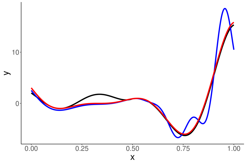
Figure 5: Visualizing the 1-d experiment: (left) the 3-node DAG used for generating the true functions; (right) the true high-fidelity (red), low-fidelity 1 (blue), and low-fidelity 2 (black) functions.

We compare 6 different predictive models here: the “high-fidelity” GP, two variants of the KO model, the NARGP (nonlinear autoregressive multi-fidelity GP regression) model (Perdikaris et al.,, 2017), and the proposed r-GMGP and d-GMGP models. For the high-fidelity GP, only the 8 points on $H$ are used for model training. Recall that a key limitation of the KO model is that the simulations (see Fig. 5 (left)) cannot be ranked from lowest to highest fidelity. To that end, two variants of the KO model are considered. The first is the KO-path model (as discussed in Section 2.2), where the KO model is fit using only data along the longest path (here, $L_{1}\rightarrow H$). The second is the KO-misspecified model, where the KO model is fit on the full simulation data with an arbitrary ordering from lowest to highest fidelity (here, $L_{2}\rightarrow L_{1}\rightarrow H$). Since the NARGP model also requires such a ranking, this model is fit on data from $L_{1}$ and $H$ (similar to KO-path). Both the proposed r-GMGP and d-GMGP models make use of the full training dataset along with the implicit DAG structure for simulation. We apply the kernel in Perdikaris et al., (2017) for NARGP, the kernel in (12) for d-GMGP, the squared-exponential kernel for the high-fidelity GP, and the Matérn-5/2 kernel for the remaining models.

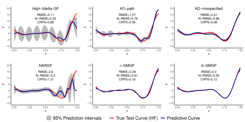
Figure 6: Results for the 1-d experiment: predictions (dark blue), 95% predictive intervals (gray) and the true high-fidelity function (red), along with its predictive metrics.

Fig. 6 compares the predictive performance of the aforementioned predictive models. We see that the proposed r-GMGP and d-GMGP models yield noticeably improved predictions over existing models, in terms of both metrics. This improvement suggests that, when the underlying graphical model dependency structure is known from prior scientific knowledge, incorporating such structure can lead to better predictive performance. Comparing the two GMGP models, we see that d-GMGP slightly outperforms r-GMGP. This is not too surprising, since from Fig. 5 (right), we see that the dependency between nodes is quite nonlinear between the low and high fidelity functions, so a more flexible (nonlinear) structure should yield improved predictive models. The online supplement reports similar results for a 5-d experiment using the same DAG.

5.2 20-dimensional experiment

We then investigate performance on a higher-dimensional problem with highly nonlinear dependencies between nodes. We use here the 5-node DAG from Fig. 2 (left), which consists of two low-fidelity functions ($L_{1}$ and $L_{2}$), two medium-fidelity functions ($M_{1}$ and $M_{2}$) and one high-fidelity function ($H$). The high-fidelity function $H$ is taken to be the $d=20$-dimensional test function from Welch et al., (1992) over design space $[-0.5,0.5]^{20}$. The medium-fidelity function $M_{1}$ is obtained by averaging $H$ over a sliding window of width $\pm 0.1x_{l}$ over each input $l=1,\cdots,20$. The low-fidelity functions $L_{1}$ and $L_{2}$ are similarly obtained by averaging $M_{1}$ over a sliding window of size $\pm 0.15x_{l}$, over the 10 odd inputs (i.e., $x_{1},\cdots,x_{19}$) for $L_{1}$, and over the 10 even inputs for $L_{2}$. This mimics the scenario where lower-fidelity functions are obtained via an averaging operation, which is widely encountered in physics (e.g., Pope,, 2000). The remaining medium-fidelity function $M_{2}$ is obtained via a simple approximation of $H$: $Z_{M_{2}}(\boldsymbol{x})=1.2Z_{H}(\boldsymbol{x})-1$. Design points for $L_{1}$, $L_{2}$, $M_{1}$, $M_{2}$ and $H$ are generated from a maximin SLHD with sample sizes 200, 200, 160, 160, and $n_{H}$, respectively, where the high-fidelity sample size $n_{H}$ increases from 40 to 120 in increments of 20. For testing, $M=500$ random test samples are used. This procedure is repeated for 20 times to account for error variability. Since dependencies between nodes are highly nonlinear, the d-GMGP is used in place of the r-GMGP model.

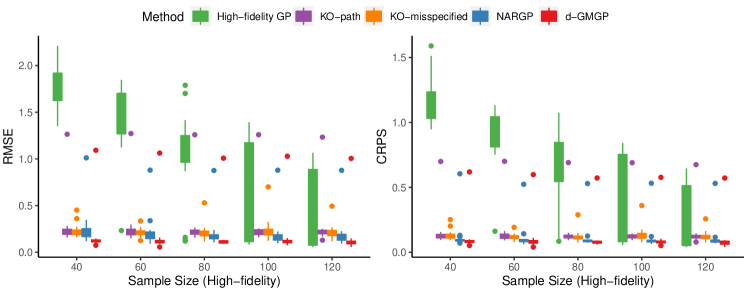
Figure 7: Results for the 20-d experiment: boxplots of two performance metrics for different sample sizes on $H$ (left: RMSE, right: CRPS).

Fig. 7 shows the boxplots of RMSE and CRPS (N-RMSE results are in the online supplement) for various high-fidelity sample sizes. There are several observations of interest. First, for all sample sizes, d-GMGP outperforms existing models, which again shows that, by leveraging the underlying model dependency structure in the form of a DAG, the proposed method can yield significant improvements in terms of predictive performance. Second, this improvement is most pronounced when the high-fidelity sample size is small. This is intuitive: as high-fidelity data become limited, additional structure linking multi-fidelity data should be more effective in improving predictive performance. Here, the d-GMGP model seems capable of leveraging this DAG dependency structure for prediction, yielding good performance even in the challenging setting where there is limited high-fidelity training data in a high-dimensional space.

5.3 Experimental design

Finally, we investigate the proposed designs from Section 4 on the earlier 1-d and 5-d problems (the latter in online supplement), which use the 3-node DAG in Fig. 5 (left). For the 1-d problem, we set the computational cost per run at each node ($L_{1}$,$L_{2}$,$H$) to be $(2,2,32)$; for the 5-d problem, this cost per run is set as $(2,2,64)$, respectively. We then compare the design methods (discussed below) on cost budgets ranging from 160 to 360 in increments of 40 for the 1-d problem, and from 600 to 1200 in increments of 100 for the 5-d problem.

The proposed design from Section 4 is compared to two baseline design approaches given a fixed computational budget $C$. The first approach allocates the full budget to the high-fidelity node $H$. A Sobol’ sequence (Joe and Kuo,, 2003) is used for the 1-d problem, and a maximin LHD (Morris and Mitchell,, 1995) is used for the 5-d problem. The second approach allocates the computational budget to the three nodes $L_{1}$, $L_{2}$ and $H$ with a fixed ratio of sample sizes. Two choices of fixed ratios are used: $6:6:1$ and $8:8:1$ for the 1-d problem, and $2:2:1$ and $3:3:1$ for the 5-d problem. The ratios are chosen such that the budget allocation is likely to be different from the proposed design. For the 1-d problem, a Sobol’ sequence is used to generate the nested designs over the DAG (see Section 4.1 for details); for the 5-d problem, a maximin SLHD (Ba et al.,, 2015) is used to generate the nested designs. We then implement the proposed design approach with moderate dependency ($\rho=0.5$ for 1-d, $\rho=0.6$ for 5-d) and high dependency ($\rho=0.9$), by first computing the desired sample size at each node via (17), then allocating the design points using the nested BFS design (Algorithm 1). The standard GP model and r-GMGP model with Matérn 5/2 kernel are then fit to the data, and the performances are compared via the RMSE of $M=100$ test points for 1-d problem and $M=500$ test points for 5-d problem. We repeat the procedure 20 times to reduce sampling variation.

Fig. 8 shows the average RMSE of the compared design approaches for the 1-d and 5-d problems. We see that, given a fixed budget $C$, the proposed designs for both moderate and high dependencies yield noticeably better predictive performance to both the high-fidelity design (where the full budget is allocated to high-fidelity runs) and the fixed ratio designs. This suggests that the proposed design approach, which jointly determines sample sizes and allocates sample points over each node in the DAG, is quite effective in reducing predictive error given a fixed budget, which is as desired. Furthermore, from these (and other) experiments, the performance of our designs appear quite robust to the choice of dependency parameter $\rho$, given it is sufficiently large (but not equal to 1). In applications where one expects a reasonable degree of dependency between simulations a priori, we would expect the proposed design with $\rho\in[0.5,0.9]$ to yield better performance over a design with arbitrarily fixed ratio, and certainly over a design with only high-fidelity samples.

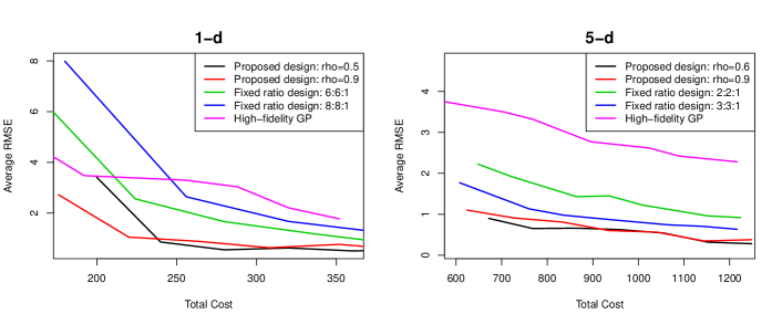
Figure 8: A comparison of average RMSE for five considered design procedures, for the 1-d problem (left) and the 5-d problem (right).

6 Multi-fidelity emulation of heavy-ion collisions

We now return to the motivating problem for emulation of heavy-ion collisions. Experiments at Brookhaven National Laboratory and the European Organization for Nuclear Research (CERN) study collisions of atomic nuclei at velocities close to the speed of light. The temperature and pressure that the colliding nuclei are subjected to in these collisions converts them into a plasma of subatomic particles. The study of nuclear collisions has increasingly employed the use of computer simulations, which involve complex scientific models that describe successively different stages of the collision. Such computer experiments are then integrated with the limited physical experimental data for calibration of unknown physical parameters. In recent years, Bayesian inference with such multi-stage simulations have led to novel discoveries on nuclear plasmas (Bernhard et al.,, 2019; Everett et al., 2021a, ; Everett et al., 2021b, ). The computational cost of these simulations is considerable, however, requiring thousands of CPU hours per run over a high-dimensional input space. This presents a crucial bottleneck for a full-scale study of nuclear collisions, and emulator models are widely used to address this computational constraint (Novak et al.,, 2014).

The computer simulators for heavy-ion collisions naturally form a multi-stage model (Everett et al., 2021b, ) as shown in Fig. 1. In our study, we consider three broad stages. The first stage models the initial impact of the two nuclei prior to hydrodynamic evolution. This pre-hydrodynamic phase can be simulated by the computationally efficient Trento model (Moreland et al.,, 2015). The second stage involves the hydrodynamic evolution of the quark-gluon-plasma. A full-fledged simulation requires numerically expensive 3D hydrodynamic modeling (which is too expensive for our study), so we neglect viscosity and consider “3+1D ideal QCD hydrodynamics” as the highest-fidelity model in this stage. This stage can be simplified by reducing the dimensionality of the hydrodynamic simulation from 3D to 1D, resulting in a lower-fidelity “1+1D ideal QCD hydrodynamics” model. A further simplification is the “1+1D linearized ideal conformal hydrodynamics” model, which replaces the equation of state of nuclear matter by a simpler conformal equation of state, and employs a linearization of the hydrodynamics equations. The third stage models the post-hydrodynamic conversion of the nuclear fluid into particles, using the Cooper-Frye prescription (Cooper and Frye,, 1974). For the observables of interest in this study, it is possible to omit this conversion in lower fidelity models. The multi-stage simulation framework is visualized in Fig. 1 and described in Everett et al., 2021b .

This multi-stage framework provides a rich testbed for multi-fidelity simulations, since experiments of different fidelities can be performed via different model combinations at each stage. After close discussions, we decided to run the following three models:

• $L_{1}$: Pre-hydrodynamics + linearized ideal conformal hydrodynamics + Cooper-Frye,

• $L_{2}$: Pre-hydrodynamics + 1+1D ideal QCD hydrodynamics,

• $H$: Pre-hydrodynamics + 3+1D ideal QCD hydrodynamics + Cooper-Frye.

Here, $H$ is the highest-fidelity model, and $L_{1}$ and $L_{2}$ are lower-fidelity representations of $H$. The corresponding DAG for this experiment is given in Fig. 5 (left).

Table 1 (left) summarizes the $d=9$ input parameters in this computer experiment, which are shared by all three simulation models. Here, we study a single output (or “observable”), which is the ratio of pions produced at rapidity $y=0$ and rapidity $y=1$. To train the emulator, we first simulate 25, 200 and 200 training points from $H$, $L_{1}$ and $L_{2}$, respectively. These design points are obtained via a maximin SLHD design (Ba et al.,, 2015), such that the design for $H$ is nested within that for $L_{1}$ and $L_{2}$ (see Section 4.1 for details). To evaluate predictive performance, $M=75$ out-of-sample testing points are generated from a separate maximin LHD design. As before, we compare the proposed r-GMGP and d-GMGP with the high-fidelity GP, the two KO model variants (KO-path and KO-misspecified), and the NARGP model in Perdikaris et al., (2017). Kernel choices for each model are the same as in earlier numerical experiments (Section 5). All models are fitted in Python, except for the r-GMGP which uses R.

Description Range nucleon width [0.35,1.40](fm) constituent width fraction [0.1,0.9] min transverse kinematic cut [0.2,1.0](GeV) fragment profile shape $\alpha$ [3.0,5.0] fragment profile shape $\beta$ [-1.0,0.0] midrapidity energy density power [0.30,0.48] midrapidity energy density normalization [0.20,0.45] fireball–fragment fluctuation [0.1,0.6] fireball profile shape [1.0,1.5]

Metrics ($\times 10^{-2}$, except N-RMSE) Computation Model RMSE N-RMSE CRPS Time (s) High-fidelity GP 5.49 0.46 3.54 2.83 KO-path 3.48 0.66 1.99 5.97 KO-misspecified 3.95 0.71 2.30 10.13 NARGP 3.66 0.73 2.13 92.15 r-GMGP 2.92 0.72 1.64 3.08 d-GMGP 2.17 0.79 1.34 135.69

Table 1: (left) $d=9$ input parameters for the heavy-ion collision simulator. (right) Predictive performance metrics and computational times for the heavy-ion collision application.

Table 1 (right) reports the predictive performance metrics and computational time for the considered emulator models. We see that the computational times for NARGP and d-GMGP models are longer than other methods, which is unsurprising since both approaches require Monte Carlo approximation. Among all six models, the proposed r-GMGP and d-GMGP give better predictive performance than existing methods, providing noticeable reductions over both test error metrics. This again suggests that, by integrating the DAG dependency structure between the simulators (i.e., the “science”) as prior knowledge, one can greatly improve predictive performance. This “science” appears to play a key role: compared to the KO-misspecified model, which misspecifies the underlying scientific connections between simulation models, the proposed GMGP models yield noticeable improvements in predictive performance by integrating model dependency information elicited from a careful inspection of the modeled physics. This can then be used for improved parameter constraints on nuclear plasma properties, leading to more precise scientific discoveries given a fixed experimental budget.

7 Conclusion

We proposed a new Graphical Multi-fidelity Gaussian Process (GMGP) model for multi-fidelity predictive modeling. The key novelty of the GMGP is the integration of scientific information in the form of a DAG, which captures connections between different simulation models in terms of fidelities. This DAG should be obtained via a careful inspection of the scientific simulation models and discussion with domain scientists. We show that the GMGP model has appealing properties for multi-fidelity modeling, and present two extensions which allow for nonlinear modeling and scalable prediction via recursive computation of the posterior predictive mean and variance at each depth level of the DAG. We also present a comprehensive experimental design methodology for the GMGP, which jointly determines the sample size on each simulation model and its corresponding design points over the parameter space. Extensive numerical experiments and an application in heavy-ion collisions demonstrate the improvement of the proposed method over existing multi-fidelity models, particularly given a tight experimental budget for simulations.

There are several interesting avenues for future work. One current limitation is that the equivalence of GMGP and r-GMGP is only shown for directed in-trees. Although this can often be satisfied via a careful design of the lower-fidelity models, it may be violated when the multi-fidelity training data are observed rather than designed. It would thus be of interest to extend this recursive formulation for more general graphs, and the incorporation of additional DAG structure under nested designs seems promising. For problems where the multi-fidelity DAG is not known with certainty, it would be useful to explore the use of DAG learning algorithms (e.g., You et al.,, 2018; Zhang et al.,, 2019) within the GMGP. Another intriguing direction would be to explore an efficient, fully Bayesian implementation that accounts for uncertainties from all model parameters; the recent work of Ma, (2020) seems to be promising for this direction. The exploration of more flexible sample sizes at different nodes is also of interest, and recent developments in flexible sliced designs (Kong et al.,, 2018) appear fruitful. Finally, in applications where model observables are highly non-stationary and/or discontinuous, the extension of the GMGP using binary tree partitions (Konomi and Karagiannis,, 2021) would be useful.

Supplementary Materials: The online supplementary materials include proofs for Propositions 1 and 2, the algorithm for d-GMGP prediction, two additional figures for the numerical experiments in Section 5, and code for reproducing Figure 6.

Acknowledgements: The authors gratefully acknowledge funding from NSF CSSI 2004571, NSF DMS 2210729, NSF DMS 2316012, DE-SC0024477 (YJ, SM), and DE-FG02-05ER41367 (SAB, JFP and DS). We also thank the JETSCAPE collaboration (https://jetscape.org/) for insightful conversations and discussions.

8 Supplementary Material

The supplementary material contains proofs for Propositions 1 and 2, the algorithm for d-GMGP prediction and two additional figures for the numerical experiments in Section 5.

9 Proof of Proposition 1

9.1 Property (a)

Property (a) can be derived from the well-known Factorization Theorem for Bayesian networks (Russell and Norvig,, 2003). Let $\{Z_{1}(\boldsymbol{x}),Z_{2}(\boldsymbol{x}),\cdots,Z_{T}(\boldsymbol{x})\}$ denote the simulation outputs with input $\boldsymbol{x}$ at all nodes on a DAG, where $Z_{t}(\boldsymbol{x})$ is the output at node $t$. By assuming a Bayesian Network structure over the DAG, the joint distribution of observations can be factorized as

$$P(Z_{1}(\boldsymbol{x}),Z_{2}(\boldsymbol{x}),\cdots,Z_{T}(\boldsymbol{x}))=\prod_{i=1}^{T}P(Z_{i}(\boldsymbol{x})|\{Z_{j}(\boldsymbol{x})\}_{j\in\text{Pa}(i)}).$$

Then, for all $Z_{t}(\boldsymbol{x})$, we have:

$$P(Z_{t}(\boldsymbol{x})|\{Z_{j}(\boldsymbol{x})\}_{j\in\text{Anc}(t)}) =\frac{P(Z_{t}(\boldsymbol{x}),\{Z_{j}(\boldsymbol{x})\}_{j\in\text{Anc}(t)})}{P(\{Z_{j}(\boldsymbol{x})\}_{j\in\text{Anc}(t)})}$$

$$=\frac{\prod_{l\in\text{Anc}(t)\cup\{t\}}P(Z_{l}(\boldsymbol{x})|\{Z_{m}(\boldsymbol{x})\}_{m\in\text{Pa}(l)})}{\prod_{l\in\text{Anc}(t)}P(Z_{l}(\boldsymbol{x})|\{Z_{m}(\boldsymbol{x})\}_{m\in\text{Pa}(l)})}$$

$$=P(Z_{t}(\boldsymbol{x})|\{Z_{j}(\boldsymbol{x})\}_{j\in\text{Pa}(t)}).$$

Thus, conditioning on parent nodes of $t$, it follows that $Z_{t}(\boldsymbol{x})$ and ancestors of $t$ that are not parent nodes are independent, i.e., $Z_{t}(\boldsymbol{x})\perp Z_{t^{\prime}}(\boldsymbol{x})|\{Z_{j}(\boldsymbol{x})\}_{j\in\textup{Pa}(t)}$ for all $t^{\prime}\neq t,t^{\prime}\notin\textup{Des}(t),t^{\prime}\notin\textup{Pa}(t)$.

9.2 Property (b)

Next, we present the proof of Property (b) for the simplest 3-node in-tree (Fig. 9). This approach can be extended analogously for more complicated in-trees.

Figure 9: Simplest 3-node in-tree.

Proof. The GMGP model for a 3-node in-tree is given as follows:

$$\begin{cases}Z_{3}(\boldsymbol{x})=\rho_{1}(\boldsymbol{x})\cdot Z_{1}(\boldsymbol{x})+\rho_{2}(\boldsymbol{x})\cdot Z_{2}(\boldsymbol{x})+\delta_{3}(\boldsymbol{x})\\ \delta_{3}(\boldsymbol{x})\perp Z_{1}(\boldsymbol{x}),\ \delta_{3}(\boldsymbol{x})\perp Z_{2}(\boldsymbol{x}),\ Z_{1}(\boldsymbol{x})\perp Z_{2}(\boldsymbol{x}).\end{cases}$$

Thus we have for $\boldsymbol{x}^{\prime}\neq\boldsymbol{x}$,

$$\text{Cov}(Z_{3}(\boldsymbol{x}),Z_{1}(\boldsymbol{x}^{\prime}))=\text{Cov}(\rho_{1}(\boldsymbol{x})\cdot Z_{1}(\boldsymbol{x}),Z_{1}(\boldsymbol{x}^{\prime}))=\rho_{1}(\boldsymbol{x})\cdot\text{Cov}(Z_{1}(\boldsymbol{x}),Z_{1}(\boldsymbol{x}^{\prime})),$$

and

$$\quad\left[\text{Cov}(Z_{3}(\boldsymbol{x}),Z_{1}(\boldsymbol{x})),\text{Cov}(Z_{3}(\boldsymbol{x}),Z_{2}(\boldsymbol{x}))\right]\begin{bmatrix}\text{Var}(Z_{1}(\boldsymbol{x}))^{-1}&0\\ 0&\text{Var}(Z_{2}(\boldsymbol{x}))^{-1}\end{bmatrix}\begin{bmatrix}\text{Cov}(Z_{1}(\boldsymbol{x}^{\prime}),Z_{1}(\boldsymbol{x}))\\ \text{Cov}(Z_{1}(\boldsymbol{x}^{\prime}),Z_{2}(\boldsymbol{x}))\end{bmatrix}$$

$$=\text{Cov}(Z_{3}(\boldsymbol{x}),Z_{1}(\boldsymbol{x}))\text{Var}(Z_{1}(\boldsymbol{x}))^{-1}\text{Cov}(Z_{1}(\boldsymbol{x}),Z_{1}(\boldsymbol{x}^{\prime}))+\text{Cov}(Z_{3}(\boldsymbol{x}),Z_{2}(\boldsymbol{x}))\text{Var}(Z_{2}(\boldsymbol{x}))^{-1}\text{Cov}(Z_{2}(\boldsymbol{x}),Z_{1}(\boldsymbol{x}^{\prime}))$$

$$=\rho_{1}(\boldsymbol{x})\cdot\text{Var}(Z_{1}(\boldsymbol{x}))\text{Var}(Z_{1}(\boldsymbol{x}))^{-1}\text{Cov}(Z_{1}(\boldsymbol{x}),Z_{1}(\boldsymbol{x}^{\prime}))+0$$

$$=\rho_{1}(\boldsymbol{x})\cdot\text{Cov}(Z_{1}(\boldsymbol{x}),Z_{1}(\boldsymbol{x}^{\prime})).$$

From the above two expressions, we have

$$\quad\ \text{Cov}(Z_{3}(\boldsymbol{x}),Z_{1}(\boldsymbol{x}^{\prime})|Z_{1}(\boldsymbol{x}),Z_{2}(\boldsymbol{x}))$$

$$=\rho_{1}(\boldsymbol{x})\cdot\text{Cov}(Z_{1}(\boldsymbol{x}),Z_{1}(\boldsymbol{x}^{\prime}))-\rho_{1}(\boldsymbol{x})\cdot\text{Cov}(Z_{1}(\boldsymbol{x}),Z_{1}(\boldsymbol{x}^{\prime}))$$

$$=0.$$

Similarly, we can show that $\text{Cov}(Z_{3}(\boldsymbol{x}),Z_{2}(\boldsymbol{x}^{\prime})|Z_{1}(\boldsymbol{x}),Z_{2}(\boldsymbol{x}))=0,\ \boldsymbol{x}^{\prime}\neq\boldsymbol{x}$. This approach can be naturally extended for general in-trees, and thus Property (b) in Proposition 1 then follows.

10 Proof of Proposition 2

We adopt an inductive approach to prove Proposition 2. In Subsection 10.1 we first show that the equivalence between the GMGP and r-GMGP model for the simplest 3-node in-tree of depth 2 (see Fig. 9), and argue that this naturally extends for in-trees of depth 2 with more than two branches (see Fig. 10). This establishes the base case for induction. In Subsection 10.2, we then show this equivalence for in-trees constructed by connecting two lower-level in-trees to a root node (see Fig. 11 (left)), and again argue that this extends for in-trees connected by more lower-level in-trees (see Fig. 11 (right)). This provides the inductive step. Finally, to complete the proof, we leverage the fact that any directed in-trees can be recursively constructed via the construction in Fig. 11 (right), thus proving the equivalence between the GMGP and r-GMGP for all directed in-trees.

10.1 Sub-graphs starting with source nodes

Proof. Let us again consider the simplest 3-node in-tree, as shown in Fig. 9. We extend the proof in Le Gratiet and Garnier, (2014) as follows. Note that the proof below naturally generalizes to the case of in-trees with multiple source nodes (see Fig. 10).

Figure 10: In-trees of depth 2 with multiple source nodes.

Let $\mathcal{D}_{s}$ be the design points at node $s,\ s=1,2,3$, and let $Z_{s}$ be the computer code at node $s$. Let $\boldsymbol{V}^{(s,s)}=\text{Var}(Z_{s}(\mathcal{D}_{s}))$ be the covariance matrix of $Z_{s}(\mathcal{D}_{s})$, and $\boldsymbol{V}_{s}$ be the full covariance matrix of the data generated by the simulators from node 1 to node $s$. With the independence assumption between codes $Z_{1}$ and $Z_{2}$, we have

$$\boldsymbol{V}_{3}=\begin{bmatrix}\boldsymbol{V}^{(1,1)}&\boldsymbol{0}&\boldsymbol{U}^{(1,3)}\\ \boldsymbol{0}&\boldsymbol{V}^{(2,2)}&\boldsymbol{U}^{(2,3)}\\ \boldsymbol{U}^{(1,3)^{T}}&\boldsymbol{U}^{(2,3)^{T}}&\boldsymbol{V}^{(3,3)}\end{bmatrix}=\begin{bmatrix}\boldsymbol{V}_{2}&\boldsymbol{U}_{2}\\ \boldsymbol{U}_{2}^{T}&\boldsymbol{V}^{(3,3)}\end{bmatrix},$$

where $\mathcal{D}_{1}$ and $\mathcal{D}_{2}$ are ordered such that $\mathcal{D}_{1}=[\mathcal{D}_{1}\setminus\mathcal{D}_{3},\mathcal{D}_{3}],\ \mathcal{D}_{2}=[\mathcal{D}_{2}\setminus\mathcal{D}_{3},\mathcal{D}_{3}]$, and $\boldsymbol{U}_{2}=\left[\boldsymbol{U}^{(1,3)},\boldsymbol{U}^{(2,3)}\right]^{T}$. Here, $\boldsymbol{U}^{(1,3)}$ and $\boldsymbol{U}^{(2,3)}$ are covariances defined as:

$$\begin{cases}\boldsymbol{U}^{(1,3)}&=\text{Cov}(Z_{1}(\mathcal{D}_{1}),Z_{3}(\mathcal{D}_{3}))=(\boldsymbol{1}_{n_{1}}\boldsymbol{\rho}_{1}(\mathcal{D}_{3})^{T})\odot\boldsymbol{V}^{(1,1)}(\mathcal{D}_{1},\mathcal{D}_{3})\\ \boldsymbol{U}^{(2,3)}&=(\boldsymbol{1}_{n_{2}}\boldsymbol{\rho}_{2}(\mathcal{D}_{3})^{T})\odot\boldsymbol{V}^{(2,2)}(\mathcal{D}_{2},\mathcal{D}_{3}),\end{cases}$$

where $\boldsymbol{V}^{(1,1)}(\mathcal{D}_{1},\mathcal{D}_{3})$ and $\boldsymbol{V}^{(2,2)}(\mathcal{D}_{2},\mathcal{D}_{3})$ contain the last $n_{3}$ columns of $\boldsymbol{V}^{(1,1)}$ and $\boldsymbol{V}^{(2,2)}$, respectively.

Thus, $\boldsymbol{V}_{2}^{-1}\boldsymbol{U}_{2}$ can be simplified to

$$\boldsymbol{V}_{2}^{-1}\boldsymbol{U}_{2} =\begin{bmatrix}(\boldsymbol{V}^{(1,1)})^{-1}&\boldsymbol{0}\\ \boldsymbol{0}&(\boldsymbol{V}^{(2,2)})^{-1}\end{bmatrix}\begin{bmatrix}\boldsymbol{U}^{(1,3)}\\ \boldsymbol{U}^{(2,3)}\end{bmatrix}=\begin{bmatrix}(\boldsymbol{1}_{n_{1}}\boldsymbol{\rho}_{1}(\mathcal{D}_{3})^{T})\odot\begin{bmatrix}\boldsymbol{0}_{(n_{1}-n_{3})\times n_{3}}\\ \boldsymbol{I}_{n_{3}}\end{bmatrix}\\ (\boldsymbol{1}_{n_{2}}\boldsymbol{\rho}_{2}(\mathcal{D}_{3})^{T})\odot\begin{bmatrix}\boldsymbol{0}_{(n_{2}-n_{3})\times n_{3}}\\ \boldsymbol{I}_{n_{3}}\end{bmatrix}\end{bmatrix}.$$

We then apply block matrix inversion to simplify $\boldsymbol{V}_{3}^{-1}$:

$$\boldsymbol{V}_{3}^{-1}=\begin{bmatrix}\boldsymbol{V}_{2}^{-1}+\boldsymbol{W}_{11}&\boldsymbol{W}_{12}\\ \boldsymbol{W}_{12}^{T}&\boldsymbol{W}_{22}\end{bmatrix}=\begin{bmatrix}\boldsymbol{V}_{2}^{-1}+\boldsymbol{V}_{2}^{-1}\boldsymbol{U}_{2}\boldsymbol{Q}_{3}^{-1}\boldsymbol{U}_{2}^{T}\boldsymbol{V}_{2}^{-1}&-\boldsymbol{V}_{2}^{-1}\boldsymbol{U}_{2}\boldsymbol{Q}_{3}^{-1}\\ -\boldsymbol{Q}_{3}^{-1}\boldsymbol{U}_{2}^{T}\boldsymbol{V}_{2}^{-1}&\boldsymbol{Q}_{3}^{-1}\end{bmatrix},$$

where

$$\quad\boldsymbol{V}_{2}^{-1} =\begin{bmatrix}(\boldsymbol{V}^{(1,1)})^{-1}&\boldsymbol{0}\\ \boldsymbol{0}&(\boldsymbol{V}^{(2,2)})^{-1}\end{bmatrix},$$

$$\boldsymbol{W}_{22} =\boldsymbol{Q}_{3}^{-1}=(\boldsymbol{V}^{(3,3)}-\boldsymbol{U}_{2}^{T}\boldsymbol{V}_{2}^{-1}\boldsymbol{U}_{2})^{-1}=\frac{1}{\sigma_{3}^{2}}\cdot\boldsymbol{R}_{3}(\mathcal{D}_{3})^{-1},$$

$$\boldsymbol{W}_{12} =-\boldsymbol{V}_{2}^{-1}\boldsymbol{U}_{2}\boldsymbol{Q}_{3}^{-1}=-\begin{bmatrix}\boldsymbol{0}_{(n_{1}-n_{3})\times n_{3}}\\ \frac{1}{\sigma_{3}^{2}}(\boldsymbol{\rho}_{1}(\mathcal{D}_{3})\boldsymbol{1}_{n_{3}}^{T})\odot\boldsymbol{R}_{3}(\mathcal{D}_{3})^{-1}\\ \boldsymbol{0}_{(n_{2}-n_{3})\times n_{3}}\\ \frac{1}{\sigma_{3}^{2}}(\boldsymbol{\rho}_{2}(\mathcal{D}_{3})\boldsymbol{1}_{n_{3}}^{T})\odot\boldsymbol{R}_{3}(\mathcal{D}_{3})^{-1}\end{bmatrix},$$

$$\boldsymbol{W}_{11} =\boldsymbol{V}_{2}^{-1}\boldsymbol{U}_{2}\boldsymbol{Q}_{3}^{-1}\boldsymbol{U}_{2}^{T}\boldsymbol{V}_{2}^{-1}$$

$$=\scalebox{0.95}{$\begin{bmatrix}\boldsymbol{0}_{(n_{1}-n_{3})\times(n_{1}-n_{3})}&\boldsymbol{0}_{(n_{1}-n_{3})\times n_{3}}&\boldsymbol{0}_{(n_{1}-n_{3})\times(n_{2}-n_{3})}&\boldsymbol{0}_{(n_{1}-n_{3})\times n_{3}}\\ \boldsymbol{0}_{n_{3}\times(n_{1}-n_{3})}&\frac{1}{\sigma_{3}^{2}}(\boldsymbol{\rho}_{1}(\mathcal{D}_{3})\boldsymbol{\rho}_{1}(\mathcal{D}_{3})^{T})\odot\boldsymbol{R}_{3}(\mathcal{D}_{3})^{-1}&\boldsymbol{0}_{n_{3}\times(n_{2}-n_{3})}&\frac{1}{\sigma_{3}^{2}}(\boldsymbol{\rho}_{1}(\mathcal{D}_{3})\boldsymbol{\rho}_{2}(\mathcal{D}_{3})^{T})\odot\boldsymbol{R}_{3}(\mathcal{D}_{3})^{-1}\\ \boldsymbol{0}_{(n_{2}-n_{3})\times(n_{1}-n_{3})}&\boldsymbol{0}_{(n_{2}-n_{3})\times n_{3}}&\boldsymbol{0}_{(n_{2}-n_{3})\times(n_{2}-n_{3})}&\boldsymbol{0}_{(n_{2}-n_{3})\times n_{3}}\\ \boldsymbol{0}_{n_{3}\times(n_{1}-n_{3})}&\frac{1}{\sigma_{3}^{2}}(\boldsymbol{\rho}_{2}(\mathcal{D}_{3})\boldsymbol{\rho}_{1}(\mathcal{D}_{3})^{T})\odot\boldsymbol{R}_{3}(\mathcal{D}_{3})^{-1}&\boldsymbol{0}_{n_{3}\times(n_{2}-n_{3})}&\frac{1}{\sigma_{3}^{2}}(\boldsymbol{\rho}_{2}(\mathcal{D}_{3})\boldsymbol{\rho}_{2}(\mathcal{D}_{3})^{T})\odot\boldsymbol{R}_{3}(\mathcal{D}_{3})^{-1}\\ \end{bmatrix}$}.$$

Next, we simplify the expression for $\boldsymbol{v}_{3}(\boldsymbol{x})^{T}\boldsymbol{V}_{3}^{-1}$, where $\boldsymbol{v}_{3}(\boldsymbol{x})$ is the covariance vector between $Z_{3}(\boldsymbol{x})$ and $\boldsymbol{z}^{(3)}=\{\boldsymbol{z}_{1},\boldsymbol{z}_{2},\boldsymbol{z}_{3}\}$ (observations at the three nodes). Then $\boldsymbol{v}_{3}(\boldsymbol{x})=\left[\boldsymbol{v}_{1}^{*}(\boldsymbol{x},\mathcal{D}_{1})^{T},\boldsymbol{v}_{2}^{*}(\boldsymbol{x},\mathcal{D}_{2})^{T},\boldsymbol{v}_{3}^{*}(\boldsymbol{x},\mathcal{D}_{3})^{T}\right]^{T}$, where

$$\begin{cases}\boldsymbol{v}_{1}^{*}(\boldsymbol{x},\mathcal{D}_{1})^{T}&=\text{Cov}(Z_{3}(\boldsymbol{x}),Z_{1}(\mathcal{D}_{1}))^{T}=\rho_{1}(\boldsymbol{x})\cdot\text{Cov}(Z_{1}(\boldsymbol{x}),Z_{1}(\mathcal{D}_{1}))^{T}=\sigma_{1}^{2}\cdot\rho_{1}(\boldsymbol{x})\cdot\boldsymbol{r}_{1}(\boldsymbol{x},\mathcal{D}_{1})^{T}\\ \boldsymbol{v}_{2}^{*}(\boldsymbol{x},\mathcal{D}_{2})^{T}&=\sigma_{2}^{2}\cdot\rho_{2}(\boldsymbol{x})\cdot\boldsymbol{r}_{2}(\boldsymbol{x},\mathcal{D}_{2})^{T}\\ \boldsymbol{v}_{3}^{*}(\boldsymbol{x},\mathcal{D}_{3})^{T}&=\boldsymbol{\rho}_{1}(\mathcal{D}_{3})\odot\boldsymbol{v}_{1}^{*}(\boldsymbol{x},\mathcal{D}_{3})^{T}+\boldsymbol{\rho}_{2}(\mathcal{D}_{3})\odot\boldsymbol{v}_{2}^{*}(\boldsymbol{x},\mathcal{D}_{3})^{T}+\sigma_{3}^{2}\cdot\boldsymbol{r}_{3}(\boldsymbol{x},\mathcal{D}_{3})^{T}.\end{cases}$$

We can thus rewrite $\boldsymbol{v}_{3}(\boldsymbol{x})^{T}\boldsymbol{V}_{3}^{-1}=\left[\boldsymbol{A},\boldsymbol{B}\right]$ where

$$\begin{cases}\boldsymbol{A}&=\left[\rho_{1}(\boldsymbol{x})\cdot\boldsymbol{v}_{1}(\boldsymbol{x})^{T}(\boldsymbol{V}^{(1,1)})^{-1},\rho_{2}(\boldsymbol{x})\cdot\boldsymbol{v}_{2}(\boldsymbol{x})^{T}(\boldsymbol{V}^{(2,2)})^{-1}\right]\\ &\quad-\left[\boldsymbol{0}_{n_{1}-n_{3}},(\boldsymbol{\rho}_{1}(\boldsymbol{x})^{T}\odot\boldsymbol{r}_{3}(\boldsymbol{x},\mathcal{D}_{3}))\boldsymbol{R}_{3}(\mathcal{D}_{3})^{-1},\boldsymbol{0}_{n_{2}-n_{3}},(\boldsymbol{\rho}_{2}(\boldsymbol{x})^{T}\odot\boldsymbol{r}_{3}(\boldsymbol{x},\mathcal{D}_{3}))\boldsymbol{R}_{3}(\mathcal{D}_{3})^{-1}\right]\\ \boldsymbol{B}&=\boldsymbol{r}_{3}(\boldsymbol{x},\mathcal{D}_{3})\boldsymbol{R}_{3}(\mathcal{D}_{3})^{-1}.\end{cases}$$

Now, we show that the mean and covariance function of the GMGP model ((6) in main paper) match that for r-GMGP ((8) in main paper). Let $\boldsymbol{H}_{3}$ be the matrix of basis functions and $\boldsymbol{\beta}=\{\boldsymbol{\beta}_{1},\boldsymbol{\beta}_{2},\boldsymbol{\beta}_{3}\}$ be the vector of coefficients such that $\boldsymbol{H}_{3}\boldsymbol{\beta}$ gives the prior mean of $\boldsymbol{z}^{(3)}$. Then $\boldsymbol{H}_{3}$ is given by:

$$\boldsymbol{H}_{3}=\begin{bmatrix}\boldsymbol{h}_{1}(\mathcal{D}_{1})^{T}&\boldsymbol{0}&\boldsymbol{0}\\ \boldsymbol{0}&\boldsymbol{h}_{2}(\mathcal{D}_{2})^{T}&\boldsymbol{0}\\ \boldsymbol{\rho}_{1}(\mathcal{D}_{3})\odot\boldsymbol{h}_{1}(\mathcal{D}_{3})^{T}&\boldsymbol{\rho}_{2}(\mathcal{D}_{3})\odot\boldsymbol{h}_{2}(\mathcal{D}_{3})^{T}&\boldsymbol{h}_{3}(\mathcal{D}_{3})^{T}\end{bmatrix}.$$

Under a similar definition, we have $\boldsymbol{H}_{1}=\boldsymbol{h}_{1}(\mathcal{D}_{1})^{T}$ and $\boldsymbol{H}_{2}=\boldsymbol{h}_{2}(\mathcal{D}_{2})^{T}$ such that the prior means of $\boldsymbol{z}_{1}$ and $\boldsymbol{z}_{2}$ are given by $\boldsymbol{H}_{1}\boldsymbol{\beta}_{1}$ and $\boldsymbol{H}_{2}\boldsymbol{\beta}_{2}$, respectively. Using the above formula for $\boldsymbol{v}_{3}(\boldsymbol{x})^{T}\boldsymbol{V}_{3}^{-1}$, we thus have

$$\boldsymbol{v}_{3}(\boldsymbol{x})^{T}\boldsymbol{V}_{3}^{-1}\boldsymbol{z}^{(3)} =\rho_{1}(\boldsymbol{x})\cdot\boldsymbol{v}_{1}(\boldsymbol{x})^{T}(\boldsymbol{V}^{(1,1)})^{-1}\boldsymbol{z}_{1}+\rho_{2}(\boldsymbol{x})\cdot\boldsymbol{v}_{2}(\boldsymbol{x})^{T}(\boldsymbol{V}^{(2,2)})^{-1}\boldsymbol{z}_{2}$$

$$\quad-(\boldsymbol{\rho}_{1}(\mathcal{D}_{3})\odot\boldsymbol{r}_{3}(\boldsymbol{x},\mathcal{D}_{3}))\boldsymbol{R}_{3}(\mathcal{D}_{3})^{-1}\boldsymbol{z}_{1}(\mathcal{D}_{3})-(\boldsymbol{\rho}_{2}(\mathcal{D}_{3})\odot\boldsymbol{r}_{3}(\boldsymbol{x},\mathcal{D}_{3}))\boldsymbol{R}_{3}(\mathcal{D}_{3})^{-1}\boldsymbol{z}_{2}(\mathcal{D}_{3})$$

$$\quad+\boldsymbol{r}_{3}(\boldsymbol{x},\mathcal{D}_{3})\boldsymbol{R}_{3}(\mathcal{D}_{3})^{-1}\boldsymbol{z}_{3},$$

$$\boldsymbol{v}_{3}(\boldsymbol{x})^{T}\boldsymbol{V}_{3}^{-1}\boldsymbol{H}_{3}\boldsymbol{\beta} =\rho_{1}(\boldsymbol{x})\cdot\boldsymbol{v}_{1}(\boldsymbol{x})^{T}(\boldsymbol{V}^{(1,1)})^{-1}\boldsymbol{H}_{1}\boldsymbol{\beta}_{1}+\rho_{2}(\boldsymbol{x})\cdot\boldsymbol{v}_{2}(\boldsymbol{x})^{T}(\boldsymbol{V}^{(2,2)})^{-1}\boldsymbol{H}_{2}\boldsymbol{\beta}_{2}$$

$$\quad+\boldsymbol{r}_{3}(\boldsymbol{x},\mathcal{D}_{3})\boldsymbol{R}_{3}(\mathcal{D}_{3})^{-1}\boldsymbol{h}_{3}(\mathcal{D}_{3})^{T}\boldsymbol{\beta}_{3},$$

$$\boldsymbol{v}_{3}(\boldsymbol{x})^{T}\boldsymbol{V}_{3}^{-1}\boldsymbol{v}_{3}({\color[rgb]{0,0,0}{\boldsymbol{x}^{\prime}}}) ={\color[rgb]{0,0,0}{\rho_{1}(\boldsymbol{x})\rho_{1}(\boldsymbol{x}^{\prime})}}\boldsymbol{v}_{1}(\boldsymbol{x})^{T}(\boldsymbol{V}^{(1,1)})^{-1}\boldsymbol{v}_{1}({\color[rgb]{0,0,0}{\boldsymbol{x}^{\prime}}})+{\color[rgb]{0,0,0}{\rho_{2}(\boldsymbol{x})\rho_{2}(\boldsymbol{x}^{\prime})}}\boldsymbol{v}_{2}(\boldsymbol{x})^{T}(\boldsymbol{V}^{(2,2)})^{-1}\boldsymbol{v}_{2}({\color[rgb]{0,0,0}{\boldsymbol{x}^{\prime}}})$$

$$\quad+\sigma_{3}^{2}\boldsymbol{r}_{3}(\boldsymbol{x},\mathcal{D}_{3})\boldsymbol{R}_{3}(\mathcal{D}_{3})^{-1}\boldsymbol{r}_{3}({\color[rgb]{0,0,0}{\boldsymbol{x}^{\prime}}},\mathcal{D}_{3})^{T}.$$

We then derive the means and variances for the r-GMGP model (equations (8) in the main paper).

$$\mu_{Z_{3}}(\boldsymbol{x}) =\left[\sum_{t^{\prime}\in Pa(3)}\rho_{t^{\prime}}(\boldsymbol{x})\boldsymbol{h}_{t^{\prime}}(\boldsymbol{x})^{T}\boldsymbol{\beta}_{t^{\prime}}+\boldsymbol{h}_{3}(\boldsymbol{x})^{T}\boldsymbol{\beta}_{3}\right]+\boldsymbol{v}_{3}(\boldsymbol{x})^{T}\boldsymbol{V}_{3}^{-1}(\boldsymbol{z}^{(3)}-\boldsymbol{H}_{3}\boldsymbol{\beta})$$

$$=\rho_{1}(\boldsymbol{x})\boldsymbol{h}_{1}(\boldsymbol{x})^{T}\boldsymbol{\beta}_{1}+\rho_{2}(\boldsymbol{x})\boldsymbol{h}_{2}(\boldsymbol{x})^{T}\boldsymbol{\beta}_{2}+\boldsymbol{h}_{3}(\boldsymbol{x})^{T}\boldsymbol{\beta}_{3}$$

$$\quad+\rho_{1}(\boldsymbol{x})\boldsymbol{v}_{1}(\boldsymbol{x})^{T}(\boldsymbol{V}^{(1,1)})^{-1}(\boldsymbol{z}_{1}-\boldsymbol{H}_{1}\boldsymbol{\beta}_{1})+\rho_{2}(\boldsymbol{x})\boldsymbol{v}_{2}(\boldsymbol{x})^{T}(\boldsymbol{V}^{(2,2)})^{-1}(\boldsymbol{z}_{2}-\boldsymbol{H}_{2}\boldsymbol{\beta}_{2})$$

$$\quad+\boldsymbol{r}_{3}(\boldsymbol{x},\mathcal{D}_{3})\boldsymbol{R}_{3}(\mathcal{D}_{3})^{-1}\left[\boldsymbol{z}_{3}-\boldsymbol{\rho}_{1}(\mathcal{D}_{3})\odot\boldsymbol{z}_{1}(\mathcal{D}_{3})-\boldsymbol{\rho}_{2}(\mathcal{D}_{3})\odot\boldsymbol{z}_{2}(\mathcal{D}_{3})-\boldsymbol{h}_{3}(\mathcal{D}_{3})^{T}\boldsymbol{\beta}_{3}\right]$$

$$=\left[\rho_{1}(\boldsymbol{x})\mu_{Z_{1}}(\boldsymbol{x})+\rho_{2}(\boldsymbol{x})\mu_{Z_{2}}(\boldsymbol{x})+\boldsymbol{h}_{3}(\boldsymbol{x})^{T}\boldsymbol{\beta}_{3}\right]$$

$$\quad+\boldsymbol{r}_{3}(\boldsymbol{x},\mathcal{D}_{3})\boldsymbol{R}_{3}(\mathcal{D}_{3})^{-1}\left[\boldsymbol{z}_{3}-\boldsymbol{\rho}_{1}(\mathcal{D}_{3})\odot\boldsymbol{z}_{1}(\mathcal{D}_{3})-\boldsymbol{\rho}_{2}(\mathcal{D}_{3})\odot\boldsymbol{z}_{2}(\mathcal{D}_{3})-\boldsymbol{h}_{3}(\mathcal{D}_{3})^{T}\boldsymbol{\beta}_{3}\right],$$

$$\sigma_{Z_{3}}^{2}(\boldsymbol{x},{\color[rgb]{0,0,0}{\boldsymbol{x}^{\prime}}}) =v^{2}_{Z_{3}}(\boldsymbol{x},{\color[rgb]{0,0,0}{\boldsymbol{x}^{\prime}}})-\boldsymbol{v}_{3}(\boldsymbol{x})^{T}\boldsymbol{V}_{3}^{-1}\boldsymbol{v}_{3}({\color[rgb]{0,0,0}{\boldsymbol{x}^{\prime}}})$$

$$={\color[rgb]{0,0,0}{\rho_{1}(\boldsymbol{x})\rho_{1}(\boldsymbol{x}^{\prime})}}\sigma_{1}^{2}+{\color[rgb]{0,0,0}{\rho_{2}(\boldsymbol{x})\rho_{2}(\boldsymbol{x}^{\prime})}}\sigma_{2}^{2}+\sigma_{3}^{2}-{\color[rgb]{0,0,0}{\rho_{1}(\boldsymbol{x})\rho_{1}(\boldsymbol{x}^{\prime})}}\boldsymbol{v}_{1}(\boldsymbol{x})^{T}(\boldsymbol{V}^{(1,1)})^{-1}\boldsymbol{v}_{1}({\color[rgb]{0,0,0}{\boldsymbol{x}^{\prime}}})$$

$$-{\color[rgb]{0,0,0}{\rho_{2}(\boldsymbol{x})\rho_{2}(\boldsymbol{x}^{\prime})}}\boldsymbol{v}_{2}(\boldsymbol{x})^{T}(\boldsymbol{V}^{(2,2)})^{-1}\boldsymbol{v}_{2}({\color[rgb]{0,0,0}{\boldsymbol{x}^{\prime}}})-\sigma_{3}^{2}\boldsymbol{r}_{3}(\boldsymbol{x},\mathcal{D}_{3})\boldsymbol{R}_{3}(\mathcal{D}_{3})^{-1}\boldsymbol{r}_{3}({\color[rgb]{0,0,0}{\boldsymbol{x}^{\prime}}},\mathcal{D}_{3})^{T}$$

$$={\color[rgb]{0,0,0}{\rho_{1}(\boldsymbol{x})\rho_{1}(\boldsymbol{x}^{\prime})}}\sigma^{2}_{Z_{1}}(\boldsymbol{x},{\color[rgb]{0,0,0}{\boldsymbol{x}^{\prime}}})+{\color[rgb]{0,0,0}{\rho_{2}(\boldsymbol{x})\rho_{2}(\boldsymbol{x}^{\prime})}}\sigma^{2}_{Z_{2}}(\boldsymbol{x},{\color[rgb]{0,0,0}{\boldsymbol{x}^{\prime}}})+\sigma_{3}^{2}\left[1-\boldsymbol{r}_{3}(\boldsymbol{x},\mathcal{D}_{3})^{T}\boldsymbol{R}_{3}(\mathcal{D}_{3})^{-1}\boldsymbol{r}_{3}({\color[rgb]{0,0,0}{\boldsymbol{x}^{\prime}}},\mathcal{D}_{3})\right].$$

With this, we can now show the equivalence of predictive means and variances (by letting $\boldsymbol{x}=\boldsymbol{x}^{\prime}$) for the GMGP and r-GMGP models (from equations (6) and (8) in the main paper):

$$\mu_{Z_{3}}(\boldsymbol{x}) =\left[\rho_{1}(\boldsymbol{x})\mu_{Z_{1}}(\boldsymbol{x})+\rho_{2}(\boldsymbol{x})\mu_{Z_{2}}(\boldsymbol{x})+\boldsymbol{h}_{3}(\boldsymbol{x})^{T}\boldsymbol{\beta}_{3}\right]$$

$$\quad+\boldsymbol{r}_{3}(\boldsymbol{x},\mathcal{D}_{3})\boldsymbol{R}_{3}(\mathcal{D}_{3})^{-1}\left[\boldsymbol{z}_{3}-\boldsymbol{\rho}_{1}(\mathcal{D}_{3})\odot\boldsymbol{z}_{1}(\mathcal{D}_{3})-\boldsymbol{\rho}_{2}(\mathcal{D}_{3})\odot\boldsymbol{z}_{2}(\mathcal{D}_{3})-\boldsymbol{h}_{3}(\mathcal{D}_{3})^{T}\boldsymbol{\beta}_{3}\right],$$

$$\sigma_{Z_{3}}^{2}(\boldsymbol{x}) =\rho_{1}^{2}(\boldsymbol{x})\sigma^{2}_{Z_{1}}(\boldsymbol{x})+\rho_{2}^{2}(\boldsymbol{x})\sigma^{2}_{Z_{2}}(\boldsymbol{x})+\sigma_{3}^{2}\left[1-\boldsymbol{r}_{3}(\boldsymbol{x},\mathcal{D}_{3})^{T}\boldsymbol{R}_{3}(\mathcal{D}_{3})^{-1}\boldsymbol{r}_{3}(\boldsymbol{x},\mathcal{D}_{3})\right].$$

As shown above, the same recursive relation holds between $\mu_{Z_{3}}(\boldsymbol{x})$ and $m_{Z_{3}}(\boldsymbol{x})$, and between $\sigma^{2}_{Z_{3}}(\boldsymbol{x})$ and $s^{2}_{Z_{3}}(\boldsymbol{x})$ when the training data are nested and noise-free. Thus we have $\mu_{Z_{3}}(\boldsymbol{x})=m_{Z_{3}}(\boldsymbol{x})$ and $\sigma^{2}_{Z_{3}}(\boldsymbol{x})=s^{2}_{Z_{3}}(\boldsymbol{x})$. With the assumption that all source nodes are independent, one can extend the proof approach in a straight-forward manner for in-trees of depth 2 with more than two source nodes.

10.2 Connecting sub-graphs

Now, let us consider a more complicated DAG which connects several lower-level in-trees. Again, we show the mean and variance equivalence using the simplest case and extend it to in-trees with more branches. Let node $A$ and $B$ be the root nodes of two lower-level in-trees, which we will call them Tree $A$ and Tree $B$, respectively. Node $A,B,C$ forms a larger in-tree and node $C$ is the child node. Fig. 11 (left) shows connections between Tree $A$ and Node $C$, Tree $B$ and Node $C$.

Figure 11: In-trees constructed by: (left) connecting $2$ lower-level in-trees; (right) connecting $M>2$ lower-level in-trees.

Again, we reorder the nested design sets such that $\mathcal{D}_{A}=[\mathcal{D}_{A}\setminus\mathcal{D}_{C},\mathcal{D}_{C}]$, $\mathcal{D}_{B}=[\mathcal{D}_{B}\setminus\mathcal{D}_{C},\mathcal{D}_{C}]$. With the independence assumption between Tree $A$ and Tree $B$, we have the following full covariance matrix:

$$\boldsymbol{V}_{C}=\begin{bmatrix}\boldsymbol{V}_{A}&\boldsymbol{0}&\boldsymbol{U}^{(A,C)}\\ \boldsymbol{0}&\boldsymbol{V}_{B}&\boldsymbol{U}^{(B,C)}\\ \boldsymbol{U}^{(A,C)^{T}}&\boldsymbol{U}^{(B,C)^{T}}&\boldsymbol{V}^{(C,C)}\end{bmatrix},$$

where $\boldsymbol{V}_{A}$ and $\boldsymbol{V}_{B}$ are covariance matrices of Tree $A$ and $B$, respectively. Let $\{Z_{A_{i}}\}_{A_{i}\in\text{Anc}(A)}$ be the non-root nodes in Tree $A$ (with $A$ being the root node), we have

$$\boldsymbol{U}^{(A,C)}=\begin{bmatrix}\text{Cov}(Z_{A_{1}}(\mathcal{D}_{A_{1}}),Z_{C}(\mathcal{D}_{C}))\\ \text{Cov}(Z_{A_{2}}(\mathcal{D}_{A_{2}}),Z_{C}(\mathcal{D}_{C}))\\ \cdots\\ \text{Cov}(Z_{A}(\mathcal{D}_{A}),Z_{C}(\mathcal{D}_{C}))\\ \end{bmatrix},$$

where

$$\text{Cov}(Z_{A_{i}}(\mathcal{D}_{A_{i}}),Z_{C}(\mathcal{D}_{C})) =\text{Cov}(Z_{A_{i}}(\mathcal{D}_{A_{i}}),\boldsymbol{\rho}_{A}(\mathcal{D}_{C})\odot Z_{A}(\mathcal{D}_{C})+\boldsymbol{\rho}_{B}(\mathcal{D}_{C})\odot Z_{B}(\mathcal{D}_{C})+\delta_{C}(\mathcal{D}_{C}))$$

$$=\text{Cov}(Z_{A_{i}}(\mathcal{D}_{A_{i}}),\boldsymbol{\rho}_{A}(\mathcal{D}_{C})\odot Z_{A}(\mathcal{D}_{C}))$$

$$=(\boldsymbol{1}_{n_{A_{i}}}\boldsymbol{\rho}_{A}(\mathcal{D}_{C})^{T})\odot\text{Cov}(Z_{A_{i}}(\mathcal{D}_{A_{i}}),Z_{A}(\mathcal{D}_{C}))$$

$$=(\boldsymbol{1}_{n_{A_{i}}}\boldsymbol{\rho}_{A}(\mathcal{D}_{C})^{T})\odot\boldsymbol{V}^{(A_{i},A)}(\mathcal{D}_{A_{i}},\mathcal{D}_{C}).$$

Thus,

$$\boldsymbol{U}^{(A,C)} =(\boldsymbol{1}_{(\sum_{A_{i}\in\text{Anc}(A)}n_{A_{i}}+n_{A})}\boldsymbol{\rho}_{A}(\mathcal{D}_{C})^{T})\odot\begin{bmatrix}\boldsymbol{V}^{(A_{1},A)}(\mathcal{D}_{A_{1}},\mathcal{D}_{C})\\ \boldsymbol{V}^{(A_{2},A)}(\mathcal{D}_{A_{2}},\mathcal{D}_{C})\\ \cdots\\ \boldsymbol{V}^{(A,A)}(\mathcal{D}_{A},\mathcal{D}_{C})\end{bmatrix}$$

$$=(\boldsymbol{1}_{(\sum_{A_{i}\in\text{Anc}(A)}n_{A_{i}}+n_{A})}\boldsymbol{\rho}_{A}(\mathcal{D}_{C})^{T})\odot\boldsymbol{V}_{A}^{n_{C}},$$

where $\boldsymbol{V}_{A}^{n_{C}}$ refers to the last $n_{C}$ columns of $\boldsymbol{V}_{A}$. With the same calculation for $\boldsymbol{U}^{(B,C)}$, we have

$$\begin{bmatrix}\boldsymbol{V}_{A}&\boldsymbol{0}\\ \boldsymbol{0}&\boldsymbol{V}_{B}\end{bmatrix}^{-1}\begin{bmatrix}\boldsymbol{U}^{(A,C)}\\ \boldsymbol{U}^{(B,C)}\end{bmatrix} =\begin{bmatrix}(\boldsymbol{1}_{(\sum_{A_{i}\in\text{Anc}(A)}n_{A_{i}}+n_{A})}\boldsymbol{\rho}_{A}(\mathcal{D}_{C})^{T})\odot\begin{bmatrix}\boldsymbol{0}_{((\sum_{A_{i}\in\text{Anc}(A)}n_{A_{i}}+n_{A})-n_{C})\times n_{C}}\\ \boldsymbol{I}_{n_{C}}\end{bmatrix}\\ (\boldsymbol{1}_{(\sum_{B_{j}\in\text{Anc}(B)}n_{B_{j}}+n_{B})}\boldsymbol{\rho}_{B}(\mathcal{D}_{C})^{T})\odot\begin{bmatrix}\boldsymbol{0}_{((\sum_{B_{j}\in\text{Anc}(B)}n_{B_{j}}+n_{B})-n_{C})\times n_{C}}\\ \boldsymbol{I}_{n_{C}}\end{bmatrix}\end{bmatrix}.$$

We observe that the above expression is comparable to $\boldsymbol{V}_{2}^{-1}\boldsymbol{U}_{2}$ defined in previous section. Similarly, using the same definition of matrix $\boldsymbol{Q}_{C}$, we see that it is comparable to $\boldsymbol{Q}_{3}$: $\boldsymbol{Q}_{C}=\text{Cov}(Z_{C}(\mathcal{D}_{C})|Tree\ A,Tree\ B)=\sigma_{C}^{2}\boldsymbol{R}_{C}(\mathcal{D}_{C})$.

Following the same derivation as in previous section, we are able to show $\mu_{Z_{C}}(\boldsymbol{x})=m_{Z_{C}}(\boldsymbol{x})$ and $\sigma_{Z_{C}}^{2}(\boldsymbol{x})=s_{Z_{C}}^{2}(\boldsymbol{x})$. The above proof can also be naturally generalized to a more complicated in-tree where we have multiple lower-level in-trees connecting to a new root node. Finally, note that all directed in-trees can be recursively constructed by connecting lower-level in-trees to a new root node. This completes the proof of the equivalence for the posterior mean and variance of GMGP and r-GMGP when the multi-fidelity DAG $\mathcal{G}$ is a directed in-tree.

11 Algorithm for d-GMGP prediction

Algorithm 1 outlines the steps for d-GMGP prediction.

Algorithm 2 Computing the posterior predictive distribution for d-GMGP

Input: Training data $\{\mathcal{D}_{t},\boldsymbol{z}_{t}\}$ over all nodes $t\in V$; Monte Carlo sample size $N$.
Output: Samples from the posterior predictive distribution for the highest-fidelity node $[Z_{T}(\boldsymbol{x})|\boldsymbol{z}^{(T)}]$.

1:Order the DAG nodes $t=1,\cdots,T$ in terms of non-increasing depth (i.e., from leaf nodes to the root node).

2:For each node $t=1,\cdots,T$:

3:      If $t\in V_{S}$ (i.e., if $t$ is a source node):

4:            Fit a GP model on $Z_{t}\sim\mathcal{GP}(0,\sigma_{t}^{2}r_{t}(\boldsymbol{x},\boldsymbol{x^{\prime}}))$ using data $\{\mathcal{D}_{t},\boldsymbol{z}_{t}\}$.

5:      Else:

6:            Compute the posterior means $\mathbb{E}[Z_{t^{\prime}}|\{\boldsymbol{z}_{m}\}_{m\in\text{Anc}(t^{\prime})},\boldsymbol{z}_{t^{\prime}}]$ at design set $\mathcal{D}_{t}$ for parent nodes $t^{\prime}\in\text{Pa}(t)$.

7:            Fit a GP model (11) on $Z_{t}$ with kernel (12) in the main paper.

8:      End If

9:End For

10:For each node $t=1,\cdots,T$:

11:      If $t\in V_{S}$ (i.e., if $t$ is a source node):

12:            Draw $N$ samples $\{z^{*}_{t,(i)}\}_{i=1}^{N}$ from the posterior distribution $[Z_{t}(\boldsymbol{x})|\boldsymbol{z}_{t}]$.

13:      Else:

14:            For $i=1,\cdots,N$, draw samples $z^{*}_{t,(i)}\sim[Z_{t}(\boldsymbol{x})|\boldsymbol{z}_{t},\{z^{*}_{t^{\prime},(i)}\}_{t^{\prime}\in\text{Pa}(t)}]$.

15:      End If

16:End For

17:Return: Monte Carlo samples $\{z^{*}_{T,(i)}\}_{i=1}^{N}$ from posterior distribution $[Z_{T}(\boldsymbol{x})|\boldsymbol{z}^{(T)}]$.

Note that the two “for” loops can be combined into one with the functionality of both fitting the model and making predictions.

12 5-dimensional experiment

In this section, we compare the performance of the different methods on a $d=5$-dimensional experiment, with the same 3-node graph as in the $d=1$-dimensional experiment. The high-fidelity function $H$ (taken from Friedman, (1991)) and the two low-fidelity functions $L_{1}$ and $L_{2}$ are given as follows:

$$\begin{cases}Z_{H}(\boldsymbol{x})=10\sin(\pi x_{1}x_{2})+20(x_{3}-0.5)^{2}+10x_{4}+5x_{5}\\ Z_{L_{1}}(\boldsymbol{x})=10\sin(4x_{1}x_{2})+20(x_{3}-0.5)^{2}+10x_{4}+5(1.2x_{5})\\ Z_{L_{2}}(\boldsymbol{x})=10\sin(3x_{1}x_{2})+20(0.8x_{3}-0.5)^{2}+10(x_{4}-0.1)+5x_{5}\end{cases}$$

The design points for $L_{1}$, $L_{2}$ and $H$ are generated from a sliced Latin Hypercube Design (SLHD, Ba et al.,, 2015) with sample sizes 40, 40 and 10, respectively, and the points in $H$ are again nested within $L_{1}$ and $L_{2}$. $M=500$ random test samples are used for comparison.

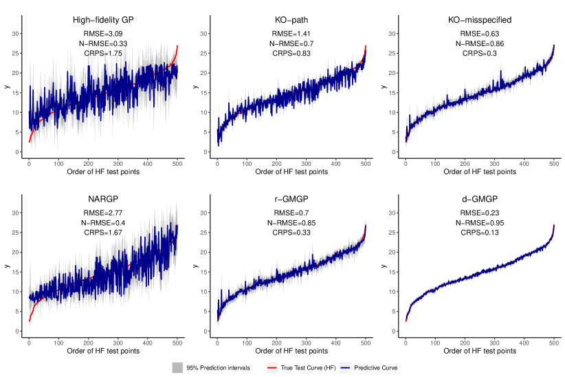
Figure 12: Results for the 5-d experiment: three predictive metrics (RMSE, N-RMSE, CRPS), predictions (dark blue), 95% predictive intervals (gray) and the true high-fidelity function (red). Here, the points are ordered from lowest to highest according to the value of high-fidelity test output.

Fig. 12 shows the predictive performance of the compared models. We see that, among the six plots, the predictive curve of the d-GMGP model is closest to the true test curve. The comparison of RMSE, N-RMSE and CRPS also shows that the proposed d-GMGP model indeed yields noticeably better predictive performance compared to other methods. This experiment again suggests that, when prior scientific information (in the form of a DAG) is available, integrating such information into a GP model can yield improved predictive performance. It is worth noting that the r-GMGP performs noticeably worse than the d-GMGP in this problem, and slightly worse than the KO-misspecified model. This is not unexpected, since again the true low and high-fidelity functions exhibit nonlinear correlations which are better captured by the d-GMGP model.

13 20-dimensional experiment

Figure 13 shows the N-RMSE comparison for the 20-d experiment. Similar to RMSE and CRPS results, d-GMGP outperforms other methods with higher N-RMSE.

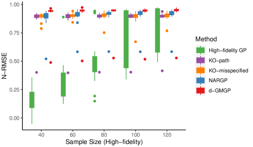
Figure 13: Results for the 20-d experiment: boxplots of N-RMSE for different sample sizes on $H$.

References

- Ba et al., (2015) Ba, S., Myers, W. R., and Brenneman, W. A. (2015). Optimal sliced Latin hypercube designs. Technometrics, 57(4):479–487.
- Bernhard et al., (2019) Bernhard, J. E., Moreland, J. S., and Bass, S. A. (2019). Bayesian estimation of the specific shear and bulk viscosity of quark–gluon plasma. Nature Physics, 15(11):1113–1117.
- Campbell and Ahmed, (2016) Campbell, M. E. and Ahmed, N. R. (2016). Distributed data fusion: neighbors, rumors, and the art of collective knowledge. IEEE Control Systems Magazine, 36(4):83–109.
- Catalano and Amato, (2003) Catalano, P. and Amato, M. (2003). An evaluation of RANS turbulence modelling for aerodynamic applications. Aerospace Science and Technology, 7(7):493–509.
- Chen et al., (2021) Chen, J., Mak, S., Joseph, V. R., and Zhang, C. (2021). Function-on-function kriging, with applications to three-dimensional printing of aortic tissues. Technometrics, 63(3):384–395.
- Cooper and Frye, (1974) Cooper, F. and Frye, G. (1974). Single-particle distribution in the hydrodynamic and statistical thermodynamic models of multiparticle production. Physical Review D, 10(1):186.
- Cutajar et al., (2019) Cutajar, K., Pullin, M., Damianou, A., Lawrence, N., and González, J. (2019). Deep Gaussian processes for multi-fidelity modeling. arXiv preprint arXiv:1903.07320.
- Damianou and Lawrence, (2013) Damianou, A. and Lawrence, N. D. (2013). Deep Gaussian processes. In Artificial Intelligence and Statistics, pages 207–215. PMLR.
- Ding et al., (2019) Ding, L., Mak, S., and Wu, C. F. J. (2019). BdryGP: a new Gaussian process model for incorporating boundary information. arXiv preprint arXiv:1908.08868.
- (10) Everett, D., Ke, W., Paquet, J.-F., Vujanovic, G., Bass, S., Du, L., Gale, C., Heffernan, M., Heinz, U., Liyanage, D., et al. (2021a). Phenomenological constraints on the transport properties of QCD matter with data-driven model averaging. Physical Review Letters, 126(24):242301.
- (11) Everett, D., Ke, W., Paquet, J.-F., Vujanovic, G., Bass, S. A., Du, L., Gale, C., Heffernan, M., Heinz, U., Liyanage, D., et al. (2021b). Multisystem Bayesian constraints on the transport coefficients of QCD matter. Physical Review C, 103(5):054904.
- Fang and Wang, (1993) Fang, K.-T. and Wang, Y. (1993). Number-Theoretic Methods in Statistics. CRC Press.
- Forrester et al., (2008) Forrester, A., Sobester, A., and Keane, A. (2008). Engineering Design via Surrogate Modelling: A Practical Guide. John Wiley & Sons.
- Friedman, (1991) Friedman, J. H. (1991). Multivariate adaptive regression splines. The Annals of Statistics, pages 1–67.
- Girard et al., (2002) Girard, A., Rasmussen, C. E., Quinonero-Candela, J., and Murray-Smith, R. (2002). Gaussian process priors with uncertain inputs - application to multiple-step ahead time series forecasting. Advances in Neural Information Processing Systems, 15:545–552.
- Gneiting and Raftery, (2007) Gneiting, T. and Raftery, A. E. (2007). Strictly proper scoring rules, prediction, and estimation. Journal of the American Statistical Association, 102(477):359–378.
- Golchi et al., (2015) Golchi, S., Bingham, D. R., Chipman, H., and Campbell, D. A. (2015). Monotone emulation of computer experiments. SIAM/ASA Journal on Uncertainty Quantification, 3(1):370–392.
- (18) Gorodetsky, A. A., Jakeman, J. D., and Geraci, G. (2020a). MFNets: learning network representations for multifidelity surrogate modeling. arXiv preprint arXiv:2008.02672.
- (19) Gorodetsky, A. A., Jakeman, J. D., Geraci, G., and Eldred, M. S. (2020b). MFNets: multi-fidelity data-driven networks for Bayesian learning and prediction. International Journal for Uncertainty Quantification, 10(6).
- Gramacy, (2020) Gramacy, R. B. (2020). Surrogates: Gaussian Process Modeling, Design, and Optimization for the Applied Sciences. CRC press.
- Harjunpää et al., (2019) Harjunpää, H., Llort Asens, M., Guenther, C., and Fagerholm, S. C. (2019). Cell adhesion molecules and their roles and regulation in the immune and tumor microenvironment. Frontiers in Immunology, 10:1078.
- Ho et al., (2022) Ho, M.-F., Bird, S., and Shelton, C. R. (2022). Multifidelity emulation for the matter power spectrum using Gaussian processes. Monthly Notices of the Royal Astronomical Society, 509(2):2551–2565.
- Joe and Kuo, (2003) Joe, S. and Kuo, F. Y. (2003). Remark on algorithm 659: Implementing Sobol’s quasirandom sequence generator. ACM Transactions on Mathematical Software (TOMS), 29(1):49–57.
- Johnson et al., (1990) Johnson, M. E., Moore, L. M., and Ylvisaker, D. (1990). Minimax and maximin distance designs. Journal of Statistical Planning and Inference, 26(2):131–148.
- Kennedy and O’Hagan, (2000) Kennedy, M. C. and O’Hagan, A. (2000). Predicting the output from a complex computer code when fast approximations are available. Biometrika, 87(1):1–13.
- Kong et al., (2018) Kong, X., Ai, M., and Tsui, K. L. (2018). Flexible sliced designs for computer experiments. Annals of the Institute of Statistical Mathematics, 70:631–646.
- Konomi and Karagiannis, (2021) Konomi, B. A. and Karagiannis, G. (2021). Bayesian analysis of multifidelity computer models with local features and nonnested experimental designs: application to the WRF model. Technometrics, 63(4):510–522.
- Korte and Vygen, (2011) Korte, B. H. and Vygen, J. (2011). Combinatorial Optimization, volume 1. Springer.
- Le Gratiet, (2012) Le Gratiet, L. (2012). MuFiCokriging: multi-fidelity cokriging models. R package version 1.2.
- Le Gratiet and Garnier, (2014) Le Gratiet, L. and Garnier, J. (2014). Recursive co-kriging model for design of computer experiments with multiple levels of fidelity. International Journal for Uncertainty Quantification, 4(5):365–386.
- López-Lopera et al., (2021) López-Lopera, A. F., Bartoli, N., Lefèvre, T., and Mouton, S. (2021). Data fusion with multi-fidelity Gaussian processes for aerodynamic experimental and numerical databases. In SIAM Conference on Computational Science and Engineering (CSE).
- Ma, (2020) Ma, P. (2020). Objective Bayesian analysis of a cokriging model for hierarchical multifidelity codes. SIAM/ASA Journal on Uncertainty Quantification, 8(4):1358–1382.
- Ma et al., (2022) Ma, P., Karagiannis, G., Konomi, B. A., Asher, T. G., Toro, G. R., and Cox, A. T. (2022). Multifidelity computer model emulation with high-dimensional output: An application to storm surge. Journal of the Royal Statistical Society Series C: Applied Statistics, 71(4):861–883.
- Mak and Joseph, (2018) Mak, S. and Joseph, V. R. (2018). Minimax and minimax projection designs using clustering. Journal of Computational and Graphical Statistics, 27(1):166–178.
- Mak et al., (2018) Mak, S., Sung, C.-L., Wang, X., Yeh, S.-T., Chang, Y.-H., Joseph, V. R., Yang, V., and Wu, C. F. J. (2018). An efficient surrogate model for emulation and physics extraction of large eddy simulations. Journal of the American Statistical Association, 113(524):1443–1456.
- Mehlhorn and Sanders, (2008) Mehlhorn, K. and Sanders, P. (2008). Algorithms and Data Structures: The Basic Toolbox, volume 55. Springer.
- Moreland et al., (2015) Moreland, J. S., Bernhard, J. E., and Bass, S. A. (2015). Alternative ansatz to wounded nucleon and binary collision scaling in high-energy nuclear collisions. Physical Review C, 92(1):011901.
- Morris and Mitchell, (1995) Morris, M. D. and Mitchell, T. J. (1995). Exploratory designs for computational experiments. Journal of Statistical Planning and Inference, 43(3):381–402.
- Nocedal and Wright, (2006) Nocedal, J. and Wright, S. (2006). Numerical Optimization. Springer Science & Business Media.
- Novak et al., (2014) Novak, J., Novak, K., Pratt, S., Vredevoogd, J., Coleman-Smith, C., and Wolpert, R. (2014). Determining fundamental properties of matter created in ultrarelativistic heavy-ion collisions. Physical Review C, 89(3):034917.
- Okuda, (1972) Okuda, H. (1972). Nonphysical noises and instabilities in plasma simulation due to a spatial grid. Journal of Computational Physics, 10(3):475–486.
- O’Hagan, (1998) O’Hagan, A. (1998). A Markov property for covariance structures. Technical report, University of Nottingham.
- Perdikaris et al., (2017) Perdikaris, P., Raissi, M., Damianou, A., Lawrence, N. D., and Karniadakis, G. E. (2017). Nonlinear information fusion algorithms for data-efficient multi-fidelity modelling. Proceedings of the Royal Society A: Mathematical, Physical and Engineering Sciences, 473(2198):20160751.
- Pilania et al., (2017) Pilania, G., Gubernatis, J. E., and Lookman, T. (2017). Multi-fidelity machine learning models for accurate bandgap predictions of solids. Computational Materials Science, 129:156–163.
- Pope, (2000) Pope, S. B. (2000). Turbulent Flows. Cambridge University Press.
- Pronzato, (2017) Pronzato, L. (2017). Minimax and maximin space-filling designs: some properties and methods for construction. Journal de la Société Française de Statistique, 158(1):7–36.
- Qian, (2012) Qian, P. Z. G. (2012). Sliced Latin hypercube designs. Journal of the American Statistical Association, 107(497):393–399.
- Russell and Norvig, (2003) Russell, S. and Norvig, P. (2003). Artificial Intelligence: A Modern Approach. Prentice Hall, second edition.
- Santner et al., (2019) Santner, T. J., Williams, B. J., and Notz, W. I. (2019). The Design and Analysis of Computer Experiments. Springer.
- Stephenson, (2000) Stephenson, T. A. (2000). An introduction to Bayesian network theory and usage. Technical report, IDIAP.
- Sung et al., (2020) Sung, C.-L., Hung, Y., Rittase, W., Zhu, C., and Wu, C. (2020). Calibration for computer experiments with binary responses and application to cell adhesion study. Journal of the American Statistical Association, 115(532):1664–1674.
- Wang, (2016) Wang, X. (2016). Swirling fluid mixing and combustion dynamics at supercritical conditions. PhD thesis, Georgia Institute of Technology.
- Wang and Berger, (2016) Wang, X. and Berger, J. O. (2016). Estimating shape constrained functions using Gaussian processes. SIAM/ASA Journal on Uncertainty Quantification, 4(1):1–25.
- Welch et al., (1992) Welch, W. J., Buck, R. J., Sacks, J., Wynn, H. P., Mitchell, T. J., and Morris, M. D. (1992). Screening, predicting, and computer experiments. Technometrics, 34(1):15–25.
- Wendland, (2004) Wendland, H. (2004). Scattered Data Approximation, volume 17. Cambridge University Press.
- Wu and Schaback, (1993) Wu, Z. and Schaback, R. (1993). Local error estimates for radial basis function interpolation of scattered data. IMA Journal of Numerical Analysis, 13(1):13–27.
- Xia et al., (2009) Xia, Y., Shang, J., Chen, J., and Liu, G.-P. (2009). Networked data fusion with packet losses and variable delays. IEEE Transactions on Systems, Man, and Cybernetics, Part B (Cybernetics), 39(5):1107–1120.
- You et al., (2018) You, J., Ying, R., Ren, X., Hamilton, W., and Leskovec, J. (2018). GraphRNN: Generating realistic graphs with deep auto-regressive models. In International Conference on Machine Learning, pages 5708–5717. PMLR.
- Zhang et al., (2019) Zhang, M., Jiang, S., Cui, Z., Garnett, R., and Chen, Y. (2019). D-VAE: A variational autoencoder for directed acyclic graphs. Advances in Neural Information Processing Systems, 32.
- Zhang et al., (2021) Zhang, R., Mak, S., and Dunson, D. (2021). Gaussian process subspace regression for model reduction. arXiv preprint arXiv:2107.04668.