Modeling and Design of IRS-Assisted Multi-Link FSO Systems

Abstract

In this paper, we investigate the modeling and design of intelligent reflecting surface (IRS)-assisted optical communication systems which are deployed to relax the line-of-sight (LOS) requirement in multi-link free space optical (FSO) systems. The FSO laser beams incident on the optical IRSs have a Gaussian power intensity profile and a nonlinear phase profile, whereas the plane waves in radio frequency (RF) systems have a uniform power intensity profile and a linear phase profile. Given these substantial differences, the results available for IRS-assisted RF systems are not applicable to IRS-assisted FSO systems. Therefore, we develop a new analytical channel model for point-to-point IRS-assisted FSO systems based on the Huygens-Fresnel principle. Our analytical model captures the impact of the size, position, and orientation of the IRS as well as its phase shift profile on the end-to-end channel. To allow the sharing of the optical IRS by multiple FSO links, we propose three different protocols, namely the time division (TD), IRS-division (IRSD), and IRS homogenization (IRSH) protocols. The proposed protocols address the specific characteristics of FSO systems including the non-uniformity and possible misalignment of the laser beams. Furthermore, to compare the proposed IRS sharing protocols, we analyze the bit error rate (BER) and the outage probability of IRS-assisted multi-link FSO systems in the presence of inter-link interference. Our simulation results validate the accuracy of the proposed analytical channel model for IRS-assisted FSO systems and confirm that this model is applicable for both large and intermediate IRS-receiver lens distances. Furthermore, we show that for the proposed IRSD and IRSH protocols, inter-link interference becomes negligible if the laser beams are properly centered on the IRS and the transceivers are carefully positioned, respectively. Moreover, in the absence of misalignment errors, the IRSD protocol outperforms the other protocols, whereas in the presence of misalignment errors, the IRSH protocol performs significantly better than the IRSD protocol.

I Introduction

Free space optical (FSO) systems are prime candidates for facilitating the bandwidth-hungry services of the next generation of wireless communication networks and beyond [2]. Due to their directional narrow laser beams, easy-to-install and cost-efficient transceivers, license-free bandwidth, and high data rate, FSO links are appealing for last-mile access, fiber backup, and backhaul of wireless networks. However, FSO systems require line-of-sight (LOS) link connections and they are impaired by atmospheric turbulence, beam divergence, and misalignment errors in long-distance deployments. To mitigate these performance-limiting factors, various methods including diversity techniques [3], serial and parallel FSO relays [4], and RF backup links [5] have been proposed. Recently, the authors of [6, 7] proposed the application of optical intelligent reflecting surfaces (IRSs) to connect a transmitter with an obstructed receiver.

Optical IRSs are planar structures which can manipulate the properties of an incident wave such as its polarization, phase, and amplitude in reflection and transmission [8, 9]. They can be realized using different technologies including mirrors, micro-mirrors, and metamaterials [10]. Mirrors and micro-mirrors only support specular reflection by mechanical adjustment of their orientation. Metamaterials consist of nano-structured antennas, referred to as unit cells, which can resonate in scales much smaller than the wavelength [10]. Thus, optical metamaterial-based IRSs can provide a better control of the spatial resolution of the reflected wave compared to mirrors and micro-mirrors. In particular, they can apply an abrupt phase shift to the incident wave, changing the accumulated phase of the wave and focusing or redirecting the wave in a desired direction.

In radio frequency (RF) wireless communication systems, IRSs have been exploited to increase coverage, ensure security, harness interference, and improve the quality of non-line-of-sight (NLOS) connections [11]. Unlike RF systems, where the wavefront incident on the IRS can be modeled as planar and the power is uniformly distributed across the IRS, FSO systems employ Gaussian laser beams, which have a curved wavefront and a non-uniform power distribution. Therefore, a careful study of IRS-assisted FSO systems is needed as existing results from IRS-assisted RF systems are not applicable. The authors of [6, 7] exploited geometric optics to determine the impact of an IRS on the performance of an FSO link but ignored the impact of the IRS size and the lens size in their three-dimensional model. They also employed an equivalent mirror-based analysis to determine the IRS phase shift profile required for anomalous reflection. In this paper, we exploit the Huygens-Fresnel principle to model the IRS-assisted FSO channel which explicitly captures the impact of the IRS phase shift profile, the IRS size, and lens size. Moreover, the authors of [12] applied an optical IRS to enhance indoor communication links. In [13], the impact of IRSs on visible light communication (VLC) was investigated. However, for VLC, non-directional beams are employed, which exhibit a different characteristic compared to the Gaussian laser beams used in FSO systems.

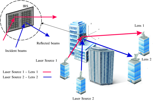
Figure 1: Multiple FSO links sharing a single IRS.

Given the Gaussian FSO beams and the flexibility of the IRS, a single IRS surface can be shared among multiple FSO links. In [14], the authors investigated point-to-multi-point FSO communications where a laser source transmits to multiple receivers based on a time-division protocol using multiple fixed reflectors and a single rotating reflector, respectively. The authors in [15] considered multi-cast transmission where a laser beam illuminates an optical IRS which splits the beam among multiple FSO receivers. They modeled the reflected power density using Fraunhofer diffraction and far-field approximations. However, we show that the far-field approximation is only valid for specific IRS-receiver lens distances, incident beam widths, and IRS tile sizes.

In this paper, we employ an IRS-assisted FSO system to provide a connection between multiple transmitters and their respective obstructed receivers, see Fig. 1. The transmitters are equipped with laser sources (LSs) emitting Gaussian beams which are reflected by an IRS towards respective receivers where the beams are focused by a lens onto a photo detector (PD). In this work, first, we develop an analytical channel model for IRS-assisted point-to-point FSO systems, then, we propose three protocols to enable the sharing of the IRS by multiple FSO links and analyze the resulting performance in terms of the bit error rate (BER) and outage probability. In the following, we summarize the main contributions of this work.

• Based on the Huygens-Fresnel principle, we analyze the deterministic channel gain of a point-to-point IRS-assisted FSO system which employs a Gaussian beam that is emitted by an LS and reflected by an optical IRS. The proposed analytical point-to-point channel model takes into account the non-uniform power distribution and the nonlinear phase profile of the Gaussian beam as well as the impact of the relative position of the IRS with respect to (w.r.t.) the lens and the LS, the size of the IRS, and the phase shift profile of the IRS.

• We show that depending on the IRS size and the width of the incident beam, existing end-to-end channel models based on the far-field approximation may not always be valid. We mathematically characterize the range of intermediate and far-field distances and propose an analytical channel model that is valid for these distances.

• Three different protocols are proposed to share a single IRS in a multi-link FSO system, namely, protocols based on time division (TD), IRS division (IRSD), and IRS homogenization (IRSH). For each protocol, the size and phase shift profile of the IRS, laser beam footprints, and the lens centers on the IRS are specified.

• We consider both linear phase shift (LP) and quadratic phase shift (QP) profiles across the IRS. The former was considered before in [16, 17, 18] and can only change the direction of the reflected beam. The latter is considered for the first time and can reduce the beam divergence along the propagation path.

• The performance of the considered multi-link FSO systems is analyzed in terms of BER and outage probability. Given that the IRS is shared by several LS-PD pairs, the inter-link interference potentially caused by the proposed IRS sharing protocols is taken into account in our analysis. Using simulations, we show that by appropriately choosing the LS-IRS and IRS-receiver lens distances as well as the separation angle between the LSs and the receiver lenses, respectively, inter-link interference can be avoided.

• Simulation results confirm our analysis of the deterministic gain of the IRS-assisted FSO channel. In particular, for large IRS sizes, large beam widths, and practical IRS-receiver lens distances, the far-field approximation may not be valid whereas our proposed model yields accurate result.

• Our simulation results also validate the analytical expressions derived for the BER and outage probability. Our results suggest that the IRSH protocol is preferable in the presence of misalignment errors. However, in the absence of misalignment errors, the IRSD protocol is advantageous as it yields a higher received power than the IRSH protocol and a lower delay compared to the TD protocol.

To the best of the authors’ knowledge, a communication-theoretical analysis of a point-to-point IRS-assisted FSO link based on the Huygens-Fresnel principle was first conducted in [1], which is the conference version of this paper. In contrast to [1], in this paper, we partition the IRS into tiles and consider not only LP profiles but also QP profiles. Moreover, multi-link FSO systems, IRS sharing protocols, and the associated analysis were not investigated in [1].

The remainder of this paper is organized as follows. The system and channel models are presented in Section II. The point-to-point IRS-assisted FSO channel gain is derived based on the Huygens-Fresnel principle in Section III. Then, in Section IV, we propose three IRS sharing protocols for multi-link FSO systems. The BER and outage probability of IRS-assisted multi-link FSO systems is analyzed in Section V. Simulation results are presented in Section VI, and conclusions are drawn in Section VII.

Notations: Boldface lower-case and upper-case letters denote vectors and matrices, respectively. Superscript $(\cdot)^{T}$ and $\mathbb{E}\{\cdot\}$ denote the transpose and expectation operators, respectively. $x\sim\mathcal{N}(\mu,\sigma^{2})$ represents a Gaussian random variable with mean $\mu$ and variance $\sigma^{2}$. $\mathbf{I}_{n}$ is the $n\times n$ identity matrix, $j$ denotes the imaginary unit, and $(\cdot)^{*}$ and $\mathcal{R}\{\cdot\}$ represent the complex conjugate and real part of a complex number, respectively. Moreover, $\text{erf}(\cdot)$ and $\text{erfi}(\cdot)$ are the error function and the imaginary error function, respectively. Furthermore, rotation matrices $\mathbf{R}_{y}({\phi})=\left(\begin{smallmatrix}\cos(\phi)&0&-\sin(\phi)\\ 0&1&0\\ \sin(\phi)&0&\cos(\phi)\end{smallmatrix}\right)$ and $\mathbf{R}_{z}({\phi})=\left(\begin{smallmatrix}\cos(\phi)&\sin(\phi)&0\\ -\sin(\phi)&\cos(\phi)&0\\ 0&0&1\end{smallmatrix}\right)$ denote the counter-clockwise rotation by angle $\phi$ around the $y$- and $z$-axes, respectively.

II System and Channel Model

We consider $N$ FSO transmitter-receiver pairs connected via a single optical IRS where each transmitter is equipped with a LS and each receiver is equipped with a PD and a lens, see Fig. 1.

II-A System Model

The IRS is installed on a building wall which we define as the $xy$-plane and the center of the IRS is at the origin, see Fig. 2. The size of the IRS is $L_{x,\text{tot}}\times L_{y,\text{tot}}$ and it consists of $Q=Q_{x}Q_{y}$ tiles, each comprising a large number of subwavelength unit cells, where $Q_{x}$ and $Q_{y}$ are the numbers of tiles in $x$- and $y$-direction, respectively. Each tile is centered at $\mathbf{r}_{q}=\left(x_{q},y_{q},0\right)$ and has length $L_{x}$ with tile spacing $l_{x}$ in $x$-direction and width $L_{y}$ with tile spacing $l_{y}$ in $y$-direction, see Fig. 2. Given that the size of a tile is much larger than the optical wavelength, i.e., $L_{x},L_{y}\gg\lambda$, each tile can be modeled as a continuous surface with a continuous phase shift profile centered at $\mathbf{r}_{q}^{t}$ and denoted by $\Phi_{q}({\mathbf{r},\mathbf{r}_{q}^{t}})$ [16], where $\mathbf{r}=(x,y,0)$ denotes a point in the $xy$-plane. Thus, the IRS length in $x$- and $y$-direction is given by $L_{i,\,\text{tot}}=Q_{i}L_{i}+(Q_{i}-1)l_{i}$, $i\in\{x,y\}$. To employ the IRS for multi-link FSO transmission, we propose different IRS sharing protocols in Section IV-A. As shown in Fig. 2, the $m$-th LS is located at distance $d_{\ell m},\,m\in\mathcal{N}$, where $\mathcal{N}=\{1,\dots,N\}$, from the center of its beam footprint on the IRS along the beam axis and its direction is denoted by $\mathbf{\Psi}_{\ell m}=\left(\theta_{\ell m},\phi_{\ell m}\right)$, where $\theta_{\ell m}$ is the angle between the $xy$-plane and the beam axis, and $\phi_{\ell m}$ is the angle between the projection of the beam axis on the $xy$-plane and the $x$-axis. For simplicity, we assume all LSs are installed at the same height as the IRS and thus, $\phi_{\ell m}=0,\,\forall m\in\mathcal{N}$, see Fig. 1. Moreover, the $m$-th laser beam footprint on the IRS plane is centered at point $\mathbf{r}_{\ell 0,m}=\left(x_{\ell 0,m},y_{\ell 0,m},0\right)$. Furthermore, we assume the $n$-th PD is equipped with a circular lens of radius $a$ with distance $d_{pn},\,n\in\mathcal{N}$, from the IRS along the normal vector of $n$-th the lens plane which has direction $\mathbf{\Psi}_{pn}=\left(\theta_{pn},\phi_{pn}\right)$, where $\theta_{pn}$ is the angle between the $xy$-plane and the normal vector, and $\phi_{pn}$ is the angle between the projection of the normal vector on the $xy$-plane and the $x$-axis. The normal vector of the $n$-th lens plane intersects the IRS plane at point $\mathbf{r}_{p0,n}=\left(x_{p0,n},y_{p0,n},0\right)$, which we refer to as the lens center on the IRS. The $n$-th lens receives a beam reflected from the IRS and focuses the beam reflected by the IRS onto its PD.

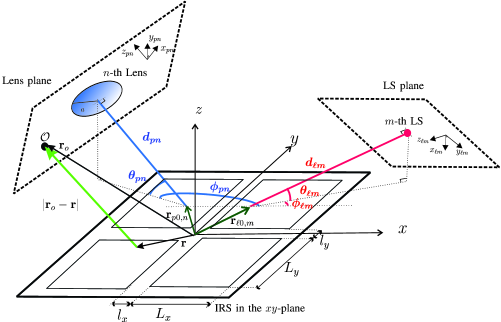
Figure 2: Schematic model of the IRS-assisted FSO system between the $m$-th LS and the $n$-th lens.

II-B Signal Model

Assuming an intensity modulation and direct detection (IM/DD) FSO system, the signal intensity $y_{n}[t]$ received by the $n$-th PD in time slot $t,t\in\mathcal{T}$, where $\mathcal{T}=\{1,\dots,T\}$, can be modeled as follows

$$y_{n}[t]=h_{n,n}s_{n}[t]+\sum_{m=1,m\neq n}^{N}h_{m,n}s_{m}[t]+w_{n}[t],\quad n\in\mathcal{N},t\in\mathcal{T},$$ (1)

where $s_{m}[t]$ is the on-off keying (OOK) modulated symbol transmitted by the $m$-th LS with average transmit power $P_{\ell m}$, $h_{m,n}\in\mathcal{R}^{+}$ is the channel gain between the $m$-th LS and the $n$-th PD, and $w_{n}[t]\sim\left(0,\sigma_{w}^{2}\right)$ is the additive white Gaussian noise (AWGN) with zero mean and variance $\sigma_{w}^{2}$ impairing the $n$-th PD.

II-C Channel Model

In general, FSO channels are affected by geometric and misalignment losses (GML), atmospheric losses, and atmospheric turbulence induced fading [19]. Thus, the IRS-assisted FSO channel gain $h_{m,n}$ between the $m$-th LS and the $n$-th PD can be modeled as follows

$$h_{m,n}=h_{p}^{m,n}h_{\text{irs}}^{m,n}h_{a}^{m,n},$$ (2)

where $h_{a}^{m,n}$ represents the random atmospheric turbulence induced fading, $h_{p}^{m,n}=10^{-\frac{\kappa}{10}(d_{\ell m}+d_{pn})}$ is the atmospheric loss which depends on the attenuation coefficient, $\kappa$, and $h_{\text{irs}}^{m,n}$ characterizes the deterministic GML. Here, we assume that the $h_{a}^{m,n},\forall m,n\in\mathcal{N}$, are independent and non-identically distributed Gamma-Gamma variables, i.e., $h_{a}^{m,n}\sim\mathcal{GG}(\alpha_{m,n},\beta_{m,n})$, with small and large scale turbulence parameters $\alpha_{m,n}$ and $\beta_{m,n}$ [20]. Moreover, $h_{\text{irs}}^{m,n}$ denotes the fraction of the power of the $m$-th LS that is reflected by the IRS and collected by the $n$-th PD, i.e.,

$$h_{\text{irs}}^{m,n}={1\over P_{\ell m}}\iint\limits_{\mathcal{A}_{pn}}I_{\text{irs}}^{m,n}\!\!\left(\mathbf{r}_{pn}\right)\,\mathrm{d}\mathcal{A}_{pn},$$ (3)

where $\mathcal{A}_{pn}$ denotes the area of the lens of the $n$-th PD, $I_{\text{irs}}^{m,n}\!\!\left(\mathbf{r}_{pn}\right)$ is the power intensity of the beam emitted by the $m$-th LS and reflected by the IRS in the plane of the $n$-th lens, and $\mathbf{r}_{pn}=(x_{pn},y_{pn},z_{pn})$ denotes a point on the lens plane. The origin of the $x_{pn}y_{pn}z_{pn}$-coordinate system is the center of the $n$-th lens and the $z_{pn}$-axis is parallel to the normal vector of the lens plane, see Fig. 2. We assume that the $y_{pn}$-axis is parallel to the intersection line of the lens plane and the IRS plane and the $x_{pn}$-axis is perpendicular to the $y_{pn}$- and $z_{pn}$-axes.

Assuming that the waist of the Gaussian laser beam, $w_{0m}$, is larger than the wavelength, $\lambda$, the paraxial approximation is valid and the power intensity of the reflected beam is given as follows [21]

$$I_{\text{irs}}^{m,n}\left(\mathbf{r}_{pn}\right)=\frac{1}{2\eta}\lvert E_{\text{irs}}^{m,n}\left(\mathbf{r}_{pn}\right)\rvert^{2},$$ (4)

where $\eta$ is the free-space impedance and $E_{\text{irs}}^{m,n}(\mathbf{r}_{pn})$ is the electric field emitted by the $m$-th LS, reflected by the IRS, and observed by the $n$-th lens. Thus, we have

$$E_{\text{irs}}^{m,n}\left(\mathbf{r}_{pn}\right)=\sum_{q=1}^{Q}E_{q}^{m,n}\left(\mathbf{r}_{pn}\right),$$ (5)

where $E_{q}^{m,n}\left(\mathbf{r}_{pn}\right)$ is the part of the electric field of the $m$-th LS which is reflected by tile $q$, see Section III. The electric field of the Gaussian laser beam emitted by the $m$-th LS is given by [22]

$$E_{\ell m}\!\left(\mathbf{r}_{\ell m}\right)= \frac{E_{0m}w_{0m}}{{w}(z_{\ell m})}\exp\left(-{x_{\ell m}^{2}+y_{\ell m}^{2}\over w^{2}(z_{\ell m})}-j\psi_{\ell m}\right)\quad\text{with phase}$$

$$\psi_{\ell m} =k\left(z_{\ell m}+{x_{\ell m}^{2}+y_{\ell m}^{2}\over 2R(z_{\ell m})}\right)-\tan^{-1}\left(\frac{z_{\ell m}}{z_{0m}}\right),\quad$$ (6)

where $\mathbf{r}_{\ell m}=(x_{\ell m},y_{\ell m},z_{\ell m})$ is a point in the coordinate system which has its origin at the $m$-th LS. The $z_{\ell m}$-axis of this coordinate system is along the beam axis, its $y_{\ell m}$-axis is parallel to the intersection line of the LS plane and the IRS plane, and its $x_{\ell m}$-axis is orthogonal to the $y_{\ell m}$- and $z_{\ell m}$-axes. Here, $E_{0m}$ is the electric field at the origin of the $x_{\ell m}y_{\ell m}z_{\ell m}$-coordinate system, $k=\frac{2\pi}{\lambda}$ is the wave number, $\lambda$ denotes the wavelength, $w(z_{\ell m})=w_{0m}\left[{1+\left(\frac{z_{\ell m}}{z_{0m}}\right)^{2}}\right]^{1/2}$ is the beam width at distance $z_{\ell m}$, $R(z_{\ell m})=z_{\ell m}\left[1+\left(\frac{z_{0m}}{z_{\ell m}}\right)^{2}\right]$ is the radius of the curvature of the beam’s wavefront, and $z_{0m}=\frac{\pi w_{0m}^{2}}{\lambda}$ is the Rayleigh range. Here, the total power emitted by the $m$-th LS is given by $P_{\ell m}=\frac{\pi}{4\eta}|E_{0m}|^{2}w^{2}_{0m}$.

III Point-to-Point Optical IRS Channel Model

In this section, we focus on a single LS-PD pair to model the impact of the IRS on the end-to-end channel. To simplify the notation, in this section, we drop the index of the LS $(m)$ and the index of the PD $(n)$ in all variables. In the following, using the electric field of the LS in (6), $E_{\ell}\left(\mathbf{r}_{\ell}\right)$, first, we determine the electric field incident on the IRS, $E_{\text{in}}(\mathbf{r})$. Then, we specify the electric field reflected from the $q$-th tile, $E_{q}\left(\mathbf{r}_{p}\right)$. Finally, we determine the total electric field reflected from the IRS and the point-to-point channel gain between the LS and the PD, $h_{\text{irs}}$.

III-A Incident Beam

First, in the following lemma, we determine the electric field incident on the IRS plane.

Lemma 1

Assuming that $d_{\ell}\gg L_{x},L_{y}$, the electric field emitted by the LS incident on the IRS plane, denoted by $E_{\text{in}}({\mathbf{r}})$, is given by

$$E_{\text{in}}({\mathbf{r}}) =\frac{E_{0}w_{0}\zeta_{\text{in}}}{{w}(\hat{d}_{\ell})}\exp\left(-{\hat{x}^{2}\over w_{x}^{2}(\hat{d}_{\ell})}-{\hat{y}^{2}\over w_{y}^{2}(\hat{d}_{\ell})}-j\psi_{\text{in}}({\mathbf{r}})\right)\quad\text{with phase}$$ (7)

$$\psi_{\text{in}}({\mathbf{r}}) =k\left(\hat{d}_{\ell}-{x}\cos(\theta_{\ell})+{\hat{x}^{2}\over 2R_{x}(\hat{d}_{\ell})}+{\hat{y}^{2}\over 2R_{y}(\hat{d}_{\ell})}\right)-\tan^{-1}\left(\frac{\hat{d}_{\ell}}{z_{0}}\right),\quad$$ (8)

where $\zeta_{\text{in}}=\sqrt{\lvert\sin(\theta_{\ell})\rvert}$, $\hat{d}_{\ell}=d_{\ell}+{x}_{\ell 0}\cos(\theta_{\ell})$, $\hat{\mathbf{r}}=\left(\hat{x},\hat{y},0\right)={\mathbf{r}}-{\mathbf{r}}_{\ell 0}$, $w_{x}(\hat{d}_{\ell})=\frac{w(\hat{d}_{\ell})}{\sin(\theta_{\ell})}$, $w_{y}(\hat{d}_{\ell})=w(\hat{d}_{\ell})$, $R_{x}(\hat{d}_{\ell})=\frac{R(\hat{d}_{\ell})}{\sin^{2}(\theta_{\ell})}$, and $R_{y}(\hat{d}_{\ell})=R(\hat{d}_{\ell})$.

Proof:

The proof is given in Appendix A. ∎

Eq. (8) describes an elliptical Gaussian beam on the IRS with beam widths $w_{x}$ and $w_{y}$ along the $x$- and $y$-axes, respectively.

III-B Huygens-Fresnel Principle

To determine the impact of the IRS on the incident beam, we use scalar field theory [22] and neglect the vectorial nature of the electromagnetic field. The scalar field approach yields accurate results if the following conditions are met: 1) the diffracting surface must be large compared to the wavelength, 2) the electromagnetic fields must not be observed very close to the surface, i.e., $d_{p}\gg\lambda$ [22]. Given the size of the IRS and the use of FSO systems for long-distance communications, these conditions are met in practice. Thus, we can apply the Huygens-Fresnel principle [22], a scalar field analysis method, for deriving the beam reflected by the IRS. This principle states that every point on the wavefront of the beam can be considered as a secondary source emitting a spherical wave and, at any position, the new wavefront is determined by the sum of these secondary waves [22]. Given this principle, the complex amplitude of the electric field reflected by the $q$-th tile, denoted by $E_{q}(\mathbf{r}_{o})$, at an arbitrary observation point $\mathcal{O}$ located at $\mathbf{r}_{o}=(x_{o},y_{o},z_{o})$, see Fig. 2, is given by [22]

$$E_{q}(\mathbf{r}_{o}) =\frac{1}{j\lambda}\iint_{({x},{y})\in\Sigma_{q}}E_{\text{in}}({\mathbf{r}})S\left({\mathbf{r}},\mathbf{r}_{o}\right)T_{q}({\mathbf{r}})\mathrm{d}{x}\mathrm{d}{y},\,\quad$$ (9)

where $S\left({\mathbf{r}},\mathbf{r}_{o}\right)={\exp(jk|\mathbf{r}_{o}-{\mathbf{r}}|)\over|\mathbf{r}_{o}-{\mathbf{r}}|}$ represents a spherical wave, see [22, Eq. (3-49)] , $T_{q}(\mathbf{r})=\zeta_{q}e^{-j\Phi_{q}({\mathbf{r},\mathbf{r}_{q}^{t}})}$ is the tile response, and $\Sigma_{q}$ is the tile area. Here, $\zeta_{q}$ denotes the efficiency factor ($0\leq\zeta_{q}\leq 1$), which accounts for the portion of incident power propagated towards the lens and $\Phi_{q}(\mathbf{r},\mathbf{r}_{q}^{t})$ is the phase shift profile of the $q$-th tile centered at $\mathbf{r}_{q}^{t}$. In (9), the total surface of the tile is divided into infinitesimally small areas $\mathrm{d}{x}\mathrm{d}{y}$, and the light wave scattered by each area is modeled as a secondary source emitting a spherical wave, modeled by ${\exp(jk|\mathbf{r}_{o}-{\mathbf{r}}|)\over|\mathbf{r}_{o}-\mathbf{r}|}$. The complex amplitudes of the secondary sources are proportional to the incident electric field, $E_{\text{in}}({\mathbf{r}})$, and an additional phase shift term, $e^{j\Phi_{q}({\mathbf{r},\mathbf{r}_{q}^{t}})}$, is introduced by the tile. The phases of the spherical sources, $k|\mathbf{r}_{o}-{\mathbf{r}}|$, play an important role in our analysis, and to find a closed-form solution for the integral in (9), we approximate $|\mathbf{r}_{o}-{\mathbf{r}}|$ in the following.

III-C Intermediate-Field vs. Far-Field

First, using $|\mathbf{r}_{o}-\mathbf{r}|=\left[({x}-x_{o})^{2}+({y}-y_{o})^{2}+z_{o}^{2}\right]^{1/2}$, we establish

$$\frac{|\mathbf{r}_{o}-{\mathbf{r}}|^{2}}{|{\mathbf{r}}_{o}|^{2}}=1+\frac{x^{2}+y^{2}}{|{\mathbf{r}}_{o}|^{2}}-2\frac{xx_{o}+yy_{o}}{|{\mathbf{r}}_{o}|^{2}}.\qquad$$ (10)

Applying the Taylor series expansion [23] with $(1+\varkappa)^{1/2}=1+\frac{1}{2}\varkappa-\frac{1}{8}\varkappa^{2}+\cdots$, we obtain

$${|\mathbf{r}_{o}-{\mathbf{r}}|} =\underbrace{|{\mathbf{r}}_{o}|-{\frac{xx_{o}+yy_{o}}{|{\mathbf{r}}_{o}|}}}_{=\text{t}_{1}}+\underbrace{\frac{x^{2}+y^{2}}{2|{\mathbf{r}}_{o}|}-\frac{x^{2}x_{o}^{2}+y^{2}y_{o}^{2}}{2|{\mathbf{r}}_{o}|^{3}}}_{=\text{t}_{2}}$$ (11)

$$-\underbrace{\frac{(x^{2}+y^{2})^{2}}{8|{\mathbf{r}}_{o}|^{3}}+\frac{(x^{2}+y^{2})(xx_{o}+yy_{o})}{2|{\mathbf{r}}_{o}|^{3}}-\frac{xyx_{o}y_{o}}{|{\mathbf{r}}_{o}|^{3}}}_{=\text{t}_{3}}+\cdots.\qquad$$

For the commonly used far-field approximation, it is assumed that the secondary waves reflected by the tile surface experience only a linear phase shift w.r.t. each other [24]. This approximation is equivalent to assuming a linear phase shift for the phase of the secondary sources w.r.t. the $x$- and $y$-directions. In other words, only $\text{t}_{1}$ in (11) is taken into account, and $\text{t}_{2}$ and all higher orders terms are neglected. For the far-field approximation to hold, the impact of $\text{t}_{2}$ in the argument of the exponential term, $k|\mathbf{r}_{o}-{\mathbf{r}}|$, should be much smaller than one period of the complex exponential, and thus,

$$k\frac{x^{2}+y^{2}}{2|\mathbf{r}_{o}|}\ll 2\pi.$$ (12)

The range of the relevant values for $x$ and $y$ in (9) is bounded by the beam widths of the incident electric field $2w_{x}$ and $2w_{y}$ (where the power of the incident beam drops by $\frac{1}{e^{4}}$ compared to the peak value) and the size of the tile $L_{x}$ and $L_{y}$, i.e., $x_{e}=\min\left(\frac{L_{x}}{2},w_{x}\right)\geq|x|$ and $y_{e}=\min\left(\frac{L_{y}}{2},w_{y}\right)\geq|y|$. Assuming that the lens radius is smaller than the IRS-lens distance, i.e., $a\ll d_{p}$, for any observation point $\mathcal{O}$ on the lens area, we can substitute $|\mathbf{r}_{o}|\approx d_{p}$. Thus, we substitute $x_{e}$ and $y_{e}$ for $x$ and $y$ in (12), respectively, and define the minimum far-field distance $d_{f}$ as follows

$$d_{f}=\frac{x_{e}^{2}+y_{e}^{2}}{2\lambda},\qquad$$ (13)

such that for distances $d_{p}\gg d_{f}$, the approximation of (11) in (9) by term $\text{t}_{1}$ only is appropriate. However, depending on the values of $x_{e}$ and $y_{e}$, and the IRS-lens distance, $d_{p}$, this condition might not hold in practice. For example, consider a typical IRS with tile size $L_{x}=L_{y}=50$ cm and a LS located at $d_{\ell}=1000$ m and $\mathbf{\Psi}_{\ell}=\left(\frac{\pi}{8},0\right)$. Then, a laser beam with wavelength $\lambda=1550$ nm and $w_{0}=2.5$ mm has widths $w_{x}=0.52$ m and $w_{y}=0.19$ m on the IRS and the minimum far-field distance according to (13) is $d_{f}=32.7$ km, which exceeds the typical link distance of FSO systems. Thus, in order to obtain a model that is also valid for shorter distances, we have to consider both the linear term $\text{t}_{1}$ and the quadratic term $\text{t}_{2}$ in (11). Using a similar method as in (12), we define intermediate distances as the range where the largest term in $\text{t}_{3}$ is smaller than a wavelength, i.e.,

$$k\frac{(x^{2}+y^{2})(xx_{o}+yy_{o})}{2|{\mathbf{r}}_{o}|^{3}}\ll 2\pi.$$ (14)

Substituting $x_{e}$ and $y_{e}$ for $x$ and $y$ and setting $x_{o}=y_{o}={|{\mathbf{r}}_{o}|\over 2}\approx{d_{p}\over 2}$, we define the minimum intermediate distances $d_{n}$ as follows

$$d_{n}=\left[\frac{(x_{e}^{2}+y_{e}^{2})(x_{e}+y_{e})}{4\lambda}\right]^{1/2}.$$ (15)

For the previous example, we obtain $d_{n}=85.6$ m which is much smaller than the practical range of link distances of FSO systems. Thus, for practical link distances $d_{p}\gg d_{n}$, the approximation of (11) in (9) by terms $\text{t}_{1}$ and $\text{t}_{2}$ is appropriate.

III-D Received Electric Field from a Tile

As mentioned previously, the Gaussian beam incident on the IRS in (8) has a nonlinear phase profile. In order to redirect the beam in a desired direction, the IRS must compensate the phase of the incident beam and apply an additional phase shift to redirect the beam. In the following theorem, we assume a QP profile across the IRS as an approximation of more general nonlinear phase shift profiles and obtain a closed-form solution for the reflected electric field in (9).

Theorem 1

Assume a QP profile centered at point $\mathbf{r}_{q}^{t}$, i.e., $\Phi_{q}^{\text{quad}}({\mathbf{r}},\mathbf{r}_{q}^{t})=k\big{(}\Phi_{q,0}+\Phi_{q,x}({x}-x_{q}^{t})$$+\Phi_{q,y}(y-y_{q}^{t})+\Phi_{q,x^{2}}({x}-x_{q}^{t})^{2}+\Phi_{q,y^{2}}({y}-y_{q}^{t})^{2}\big{)}$, where $\Phi_{q,0}$, $\Phi_{q,x}$, $\Phi_{q,x^{2}}$, $\Phi_{q,y}$, and $\Phi_{q,y^{2}}$ are constants. Then, the electric field emitted by the LS at position $\left(d_{\ell},\mathbf{\Psi}_{\ell}\right)$, reflected by the tile centered at $\mathbf{r}_{q}=\left(x_{q},y_{q},0\right)$, and received at the lens located at $\left(d_{p},\mathbf{\Psi}_{p}\right)$ for any intermediate distances $d_{\ell}\gg L_{x},L_{y}$ and $d_{p}\gg a,x_{\ell 0},y_{\ell 0},d_{n}$ is given by

$$E_{q}(\mathbf{r}_{p})={CC_{q}}{\frac{\pi}{4\sqrt{b_{x}b_{y}}}}\,e^{-\frac{k^{2}}{4b_{x}}X^{2}-\frac{k^{2}}{4b_{y}}Y^{2}}$$

$$\times\Bigg{[}\text{erf}\left({\sqrt{b_{x}}}\left(x_{q}+\frac{L_{x}}{2}\right)+\frac{jk}{2\sqrt{b_{x}}}X\right)-\text{erf}\left({\sqrt{b_{x}}}\left(x_{q}-\frac{L_{x}}{2}\right)+\frac{jk}{2\sqrt{b_{x}}}X\right)\Bigg{]}$$

$$\times\Bigg{[}\text{erf}\left({\sqrt{b_{y}}}\left(y_{q}+\frac{L_{y}}{2}\right)+\frac{jk}{2\sqrt{b_{y}}}Y\right)-\text{erf}\left({\sqrt{b_{y}}}\left(y_{q}-\frac{L_{y}}{2}\right)+\frac{jk}{2\sqrt{b_{y}}}Y\right)\Bigg{]},\quad$$ (16)

where $X=A_{0}+c_{1}x_{p}+c_{2}y_{p}+\Phi_{q,x}-2x_{q}^{t}\Phi_{q,x^{2}}$, $A_{0}={2j\nu{x}_{\ell 0}\over k}\sin^{2}(\theta_{\ell})+\frac{{x}_{p0}}{d_{p}}+\varphi_{x}$, $Y=B_{0}+c_{3}x_{p}+c_{4}y_{p}+\Phi_{q,y}-2y_{q}^{t}\Phi_{q,y^{2}}$, $B_{0}={2j\nu{y}_{\ell 0}\over k}+\frac{{y}_{p0}}{d_{p}}+\varphi_{y}$, $c_{1}=\frac{1}{d_{p}}\cos(\phi_{p})\sin(\theta_{p})$, $c_{2}=-\frac{1}{d_{p}}\sin(\phi_{p})$, $c_{3}=\frac{1}{d_{p}}\sin(\phi_{p})\sin(\theta_{p})$, $c_{4}=\frac{1}{d_{p}}\cos(\phi_{p})$, $c_{5}=\frac{1}{d_{p}}\cos(\phi_{p})\cos(\theta_{p})$, $c_{6}=\frac{1}{d_{p}}\sin(\phi_{p})\cos(\theta_{p})$, $\varphi_{x}=-\cos(\theta_{\ell})-\cos(\theta_{p})\cos(\phi_{p})$, $\varphi_{y}=-\cos(\theta_{p})\sin(\phi_{p})$, $b_{x}=\nu\sin^{2}(\theta_{\ell})-\frac{jk}{2d_{p}}\left(1-c_{5}^{2}d_{p}^{2}-2c_{5}x_{p0}\right)-jk\Phi_{q,x^{2}}$, $b_{y}=\nu-\frac{jk}{2d_{p}}\left(1-c_{6}^{2}d_{p}^{2}-2c_{6}y_{p0}\right)-jk\Phi_{q,y^{2}}$, $\delta_{q}=-\Phi_{q,x^{2}}(x_{q}^{t})^{2}-\Phi_{q,y^{2}}(y_{q}^{t})^{2}+\Phi_{q,x}x_{q}^{t}+\Phi_{q,y}y_{q}^{t}-\Phi_{q,0}$, $C_{q}=\zeta_{q}e^{jk\delta_{q}}$, $\nu={1\over w^{2}(\hat{d}_{\ell})}+{jk\over 2R(\hat{d}_{\ell})}$, $C=\frac{E_{o}w_{0}\zeta_{\text{in}}}{j\lambda{w}(\hat{d}_{\ell})d_{p}}e^{-jk(\hat{d}_{\ell}-d_{p})+j\tan^{-1}\left(\frac{\hat{d}_{\ell}}{z_{0}}\right)-\nu\sin^{2}(\theta_{\ell}){x}_{\ell 0}^{2}-\nu{y}_{\ell 0}^{2}}$.

Proof:

The proof is given in Appendix B. ∎

Eq. (16) explicitly shows the impact of the positioning of the LS and the lens w.r.t. the IRS, the size of the tile, and the phase shift configuration across the tile on the electric field reflected by the tile. The above theorem is valid for both far-field and intermediate distances. The electric field for LP profiles is included in the result in (16) as a special case for $\Phi_{{q,x^{2}}}=\Phi_{{q,y^{2}}}=0$, see Section IV-B for more details on the tile phase shift configuration.

In the following corollary, as a special case of Theorem 1, we consider the conventional mirror. A conventional mirror introduces no additional phase shifts, i.e., $\Phi_{q}({\mathbf{r}},\mathbf{r}_{q}^{t})=0$, and the incident angle and the reflection angle follow Snell’s law, i.e., $\theta_{\ell}=\theta_{p}$.

Corollary 1 (Reflection by Conventional Mirror)

Assume a large conventional mirror or equivalently a large tile of an IRS, i.e., ${L_{x}},L_{y}\gg 2w(\hat{d_{\ell}})$, such that the entire received beam is reflected. Then, assuming a far-field scenario, $d_{p}\gg d_{f}$, $\phi_{p}=\pi$, and $x_{\ell 0}=y_{\ell 0}=0$, (16) simplifies to

$$E_{q}(\mathbf{r}_{p}) =\frac{E_{0}w_{0}\zeta_{t}}{w_{\text{cir}}}\exp\left(-\frac{x_{p}^{2}+y_{p}^{2}}{w_{\text{cir}}^{2}}-j\psi_{\text{cir}}\right)\text{with phase}$$ (17)

$$\psi_{\text{cir}}=k\left(\hat{d}_{\ell}-d_{p}-\frac{x_{p}^{2}}{2R_{\text{cir}}}-\frac{y_{p}^{2}}{2R_{\text{cir}}}\right)+\frac{\pi}{2}-\tan^{-1}\left(\frac{\hat{d}_{\ell}}{z_{0}}\right),$$

where $\zeta_{t}=\frac{\zeta_{\text{in}}\zeta_{q}}{|\sin(\theta_{\ell})|}$, and $w_{\text{cir}}=\frac{2w(\hat{d}_{\ell})|\nu|d_{p}}{k}$ and $R_{\text{cir}}=\frac{4d_{p}^{2}|\nu|^{2}R(\hat{d}_{\ell})}{k^{2}}$ are the equivalent circular beamwidth and radius of curvature, respectively.

Proof:

Considering ${L_{x}},L_{y}\gg 2w(\hat{d}_{\ell})$, we can substitute the $\text{erf}(\cdot)$-terms in (16) by 4. Assuming $d_{p}\gg d_{f}$, we obtain $b_{x}=\nu\sin^{2}(\theta_{\ell})$ and $b_{y}=\nu$. Substituting $\theta_{\ell}=\theta_{p}$, $\phi_{p}=\pi$, and $\Phi_{q}({\mathbf{r}},\mathbf{r}_{q}^{t})=0$ leads to (17) and this completes the proof. ∎

Eq. (17) corresponds to a circular Gaussian beam, and reveals that, in the considered regime, the reflected beam is identical to what is expected from geometric optics for a conventional mirror, see [6, 7].

Corollary 2 (Reflection by Anomalous Mirror)

We assume an anomalous mirror which can impose an additional linear phase shift, i.e., $\Phi_{q,0}=0$, $\Phi_{q,x}=\cos(\theta_{\ell})\cos(\phi_{\ell})+\cos(\theta_{p})\cos(\phi_{p})$, $\Phi_{q,y}=\cos(\theta_{\ell})\sin(\phi_{\ell})+\cos(\theta_{p})\cos(\phi_{p})$, $\Phi_{q,x^{2}}=\Phi_{q,y^{2}}=0$. Then, for the far-field scenario, i.e., $d_{p}\gg d_{f}$, ${L_{x}},L_{y}\gg 2w(\hat{d_{\ell}})$, and $x_{\ell 0}=y_{\ell 0}=0$, (16) simplifies to

$$E_{q}(\mathbf{r}_{p}) =\frac{E_{0}w_{0}\zeta_{t}}{\sqrt{w_{x,\text{elp}}w_{y,\text{elp}}}}\sqrt{\frac{\sin(\theta_{\ell})}{\sin(\theta_{p})}}\exp\left(-\frac{x_{p}^{2}}{w_{x,\text{elp}}^{2}}-\frac{y_{p}^{2}}{w^{2}_{y,\text{elp}}}-j\psi_{\text{elp}}\right)\text{with phase}$$ (18)

$$\psi_{\text{elp}}=k\left(\hat{d}_{\ell}-d_{p}-\frac{x_{p}^{2}}{2R_{x,\text{elp}}}-\frac{y_{p}^{2}}{2R_{y,\text{elp}}}\right)+\frac{\pi}{2}-\tan^{-1}\left(\frac{\hat{d}_{\ell}}{z_{0}}\right),$$

where $w_{x,\text{elp}}=\frac{w_{y,\text{elp}}|\sin(\theta_{\ell})|}{|\sin(\theta_{p})|}$, $w_{y,\text{elp}}=\frac{2|\nu|d_{p}w(\hat{d}_{\ell})}{k}$, $R_{x,\text{elp}}=\frac{R_{y,\text{elp}}\sin^{2}(\theta_{\ell})}{\sin^{2}(\theta_{p})}$, and $R_{y,\text{elp}}=\frac{4d_{p}^{2}|\nu|^{2}R(\hat{d}_{\ell})}{k^{2}}$.

Proof:

Substituting $\Phi_{q,x}$ and $\Phi_{q,y}$ in (16) and following similar steps as in the proof of Corollary 1 but for the general case $\theta_{\ell}\neq\theta_{p}$ leads to (18). This completes the proof. ∎

Eq. (18) describes an elliptical Gaussian beam. This result is in agreement with the result from geometric optics for anomalous reflection [7].

Depending on the tile size, distances $d_{p}\gg d_{f}$ might not be in the practical range of FSO systems, see Section VI. Therefore, Corollaries 1 and 2, which are valid if the far-field approximation holds, do not always provide accurate results. Thus, in general, Theorem 1 is required to determine the electric field for practical applications. Moreover, by choosing appropriate values for $\Phi_{q,i}$, $i\in\{0,x,y,x^{2},y^{2}\}$ for the QP profile across the tile in (16), we can redirect the reflected electric field in a desired direction and reduce the divergence of the beam along the propagation path, see Section IV-B.

III-E Point-to-Point GML

In the previous subsection, we have determined the electric field reflected from a tile centered at $\mathbf{r}_{q}$ with phase shift profile $\Phi_{q}({\mathbf{r}},\mathbf{r}_{q}^{t})$ across the tile. Now, using (16), (5), and the power intensity in (4), the deterministic GML in (3) can be rewritten as follows

$$h_{\text{irs}}=\frac{1}{2\eta P_{\ell}}\iint_{\mathcal{A}_{p}}\Big{\lvert}\sum_{q=1}^{Q}E_{q}\left(\mathbf{r}_{p}\right)\Big{\rvert}^{2}\mathrm{d}\mathcal{A}_{p}.$$ (19)

In the following theorem, we simplify (19) and determine $h_{\text{irs}}$.

Theorem 2 (Out-of-Plane Reflection)

Assume $d_{\ell}\gg L_{x},L_{y}$ and $d_{p}\gg a,x_{\ell 0},y_{\ell 0},d_{n}$. Then, the point-to-point deterministic GML, $h_{\text{irs}}$, including geometric and deterministic misalignment losses, between an LS at position $\left(d_{\ell},\mathbf{\Psi}_{\ell}\right)$ illuminating an IRS in the $xy$-plane and a receiver lens at position $\left(d_{p},\mathbf{\Psi}_{p}\right)$ is given by

$$h^{\text{out}}_{\text{irs}}= \frac{{C}_{h}\sqrt{\pi}}{2\sqrt{\rho_{x}}}\sum\limits_{q=1}^{Q}\!\sum\limits_{\varsigma=1}^{Q}C_{q}C_{\varsigma}^{*}C_{2,q}C_{2,\varsigma}^{*}\exp\!\left(\!-\frac{k^{2}}{4}\left(\frac{{A}_{q}^{2}}{b_{x}}+\frac{{A}_{\varsigma}^{2}}{{b}_{x}^{*}}+\frac{{B}_{q}^{2}}{b_{y}}+\frac{{B}_{\varsigma}^{2}}{{b}_{y}^{*}}\right)\!\right)\int\limits_{-\tilde{a}}^{\tilde{a}}e^{-\rho_{y}y_{p}^{2}-\varrho_{y}y_{p}+\frac{(\rho_{xy}y_{p}+\varrho_{x})^{2}}{4\rho_{x}}}$$ (20)

$$\times\Big{[}\text{erf}\left(\frac{{\rho_{x}\sqrt{\pi}a}+\rho_{xy}y_{p}+\varrho_{x}}{2\sqrt{\rho_{x}}}\right)\!-\text{erf}\left(\frac{{-\rho_{x}\sqrt{\pi}a}+\rho_{xy}y_{p}+\varrho_{x}}{2\sqrt{\rho_{x}}}\right)\Big{]}\mathrm{d}y_{p},\quad$$

where $\tilde{a}=\frac{\sqrt{\pi}a}{2}$, $\tilde{b_{i}}={b_{i}{b}_{i}^{*}\over b_{i}+{b}_{i}^{*}},$ $i\in\{x,y\}$, $C_{h}\!=\!\frac{\pi\zeta^{2}_{\text{in}}}{8{|b_{x}||b_{y}|}\lambda^{2}d_{p}^{2}w^{2}(\hat{d}_{\ell})}e^{-\frac{2x_{\ell 0}^{2}\sin(\theta_{\ell})}{w^{2}(\hat{d}_{\ell})}-\frac{2y_{\ell 0}^{2}}{w^{2}(\hat{d}_{\ell})}}$, $\rho_{x}=\frac{k^{2}}{4}\left(\frac{c_{1}^{2}}{\tilde{b}_{x}}+\frac{c_{3}^{2}}{\tilde{b}_{y}}\right)$, $\rho_{y}=\frac{k^{2}}{4}\left(\frac{c_{2}^{2}}{\tilde{b}_{x}}+\frac{c_{4}^{2}}{\tilde{b}_{y}}\right)$, $\rho_{xy}=\frac{k^{2}}{2}\left(\frac{c_{1}c_{2}}{\tilde{b}_{x}}+\frac{c_{3}c_{4}}{\tilde{b}_{y}}\right)$, ${A}_{i}=A_{0}+\Phi_{i,x}-2x_{i}^{t}\Phi_{i,x^{2}}$, ${B}_{i}=B_{0}+\Phi_{i,y}-2y_{i}^{t}\Phi_{i,y^{2}}$, $\varrho_{x}=\frac{k^{2}}{2}\left(c_{1}\left(\frac{{A}_{q}}{b_{x}}+\frac{{A}_{\varsigma}^{*}}{{b}_{x}^{*}}\right)+c_{3}\left(\frac{{B}_{q}}{b_{y}}+\frac{{B}_{\varsigma}^{*}}{{b}_{y}^{*}}\right)\right)$, $\varrho_{y}=\frac{k^{2}}{2}\left(c_{2}\left(\frac{{A}_{q}}{b_{x}}+\frac{{A}_{\varsigma}^{*}}{{b}_{x}^{*}}\right)+c_{4}\left(\frac{{B}_{q}}{b_{y}}+\frac{{B}_{\varsigma}^{*}}{{b}_{y}^{*}}\right)\right)$, $C_{2,i}=\left(\text{erf}\left(\sqrt{b_{x}}{L}_{x}-\varpi_{x,i}\right)-\text{erf}\left(-\varpi_{x,i}\right)\right)$$\left(\text{erf}\left(\sqrt{b_{y}}{L}_{y}-\varpi_{y,i}\right)-\text{erf}\left(-\varpi_{y,i}\right)\right)$, $\varpi_{x,i}={\sqrt{b_{x}}}\left(\frac{L_{x}}{2}-x_{i}\right)-\frac{jk}{2\sqrt{b_{x}}}\left(A_{0}+\left(c_{1}+c_{2}\right)\frac{a}{2}+\Phi_{i,x}-2x_{i}^{t}\Phi_{i,x^{2}}\right)$, $\varpi_{y,i}\!=\!\!{\sqrt{b_{y}}}\left(\frac{L_{y}}{2}-y_{i}\right)-\frac{jk}{2\sqrt{b_{y}}}\big{(}B_{0}+\left(c_{3}+c_{4}\right)\frac{a}{2}+\Phi_{i,y}-2y_{i}^{t}\Phi_{i,y^{2}}\big{)}$, $i\!\!\in\!\!\{q,\varsigma\}$.

Proof:

The proof is given in Appendix C. ∎

Eq. (20) specifies the deterministic GML and includes a finite-range integral that can be evaluated numerically. The normal vector of the LS plane and the normal vector of the lens plane may lie in different planes, which is referred to as “out-of-plane reflection” [25]. This is in contrast to Snell’s law which states that the reflected and the incident beam are in the same plane with $\theta_{\ell}=\theta_{p}$. However, depending on the chosen phase shift profile across the IRS, the direction of the reflected beam can be outside the incident beam plane. Moreover, (20) characterizes the dependence of the channel gain on the tile size, $L_{x}$ and $L_{y}$, the phase shift profile across the tiles, $\Phi_{q}({\mathbf{r}},\mathbf{r}_{q}^{t})$, the lens radius, $a$, and the lens and LS positions and orientations, $\mathbf{r}_{\ell},\mathbf{\Psi}_{\ell}$ and $\mathbf{r}_{p},\mathbf{\Psi}_{p}$, respectively. Furthermore, variables $A_{0}$ and $B_{0}$ defined in Theorem 1 depend on the position of the center of the beam footprint on the IRS surface, $x_{\ell 0}$ and $y_{\ell 0}$, and the position where the normal vector of the lens intersects the IRS, $x_{p0}$ and $y_{p0}$, which in turn affects the GML and the end-to-end channel gain. In other words, to maximizes the received power due to the non-uniform power distribution across the IRS, the positions of the beam footprint and the lens center on the IRS should coincide. However, in case of misalignment, i.e., when the LS or the lens are not accurately tracked, only a fraction of the total power is received. We denote the corresponding misalignment error by $\mathbf{r}_{e}=|\mathbf{r}_{\ell 0}-\mathbf{r}_{p0}|$ and investigate its impact on performance in Section VI.

In the following corollary, we simplify (20), for the case where the normal vector of the LS plane and the normal vector of the lens plane lie in the same plane, e.g., the LS and the lens are at the same height, which is referred to as “in-plane-reflection” [25].

Corollary 3 (In-Plane Reflection)

For in-plane reflection, $\phi_{p}=\pi-\phi_{\ell}$ holds, and the deterministic GML simplifies to

$$h^{\text{in}}_{\text{irs}} =\frac{C_{h}\pi}{4\sqrt{\rho_{x}\rho_{y}}}\sum\limits_{q=1}^{Q}\!\sum\limits_{\varsigma=1}^{Q}C_{q}C_{\varsigma}^{*}C_{2,q}C_{2,\varsigma}^{*}\exp\left(\frac{\varrho_{x}^{2}}{4\rho_{x}}+\frac{\varrho_{y}^{2}}{4\rho_{y}}\right)$$ (21)

$$\times\left[\text{erf}\left(\sqrt{\rho_{x}}\tilde{a}+\frac{\varrho_{x}}{2\sqrt{\rho_{x}}}\right)-\text{erf}\left(-\sqrt{\rho_{x}}\tilde{a}+\frac{\varrho_{x}}{2\sqrt{\rho_{x}}}\right)\right]$$

$$\times\left[\text{erf}\left(\sqrt{\rho_{y}}\tilde{a}+\frac{\varrho_{y}}{2\sqrt{\rho_{y}}}\right)-\text{erf}\left(-\sqrt{\rho_{y}}\tilde{a}+\frac{\varrho_{y}}{2\sqrt{\rho_{y}}}\right)\right].\,\qquad$$

Proof:

Since we previously assumed $\phi_{\ell}=0$, $\phi_{p}=\pi$ holds, and the parameters in Theorem 2 simplify to $\rho_{x}=\frac{k^{2}}{2d_{p}^{2}\tilde{b}_{x}}\sin^{2}(\theta_{p})$, $\rho_{y}=\frac{k^{2}}{2d_{p}^{2}\tilde{b}_{y}}$, $\rho_{xy}=0$, $\varrho_{x}=\frac{k^{2}\sin(\theta_{p})}{2d_{p}}\left(\frac{{A}_{q}}{b_{x}}+\frac{{A}_{\varsigma}^{*}}{{b}_{x}^{*}}\right)$, and $\varrho_{y}=\frac{k^{2}}{2d_{p}}\left(\frac{{B}_{q}}{b_{y}}+\frac{{B}_{\varsigma}^{*}}{{b}_{y}^{*}}\right)$. Substituting these values, the integral in (45) simplifies to two independent integrals, which can be solved by applying [23, Eq. (2.33-1)]. Then, we obtain (21) and this completes the proof. ∎

The results in Theorem 1 and 2 are valid for a given IRS-based FSO link. To apply the above results to the IRS-based FSO link between the $m$-th LS and the $n$-th PD, we add the index of the LS $(m)$ and the index of the PD $(n)$ to all variables with index $(\ell)$ and $(p)$, respectively. Thus, we obtain the deterministic GML, $h_{\text{irs}}^{m,n}$. Based on our analysis in this section, we design optical IRSs for multi-link FSO systems in the following section.

IV IRS-Assisted Multi-Link FSO Systems

In the following, we assume multiple LSs are connected via IRS-assisted FSO links to multiple PDs. First, we propose three protocols for sharing the IRS surface between multiple FSO links, namely the TD, IRSD, and IRSH protocols, see Fig. 3. These protocols differ in their susceptibility to misalignment errors, the introduced delay, and the achieved signal-to-noise ratio (SNR), as will be shown in Section VI. For each protocol, we first specify the required number of tiles, $Q$, the location of the center of the LS beam footprint on the IRS, $\mathbf{r}_{\ell 0}$, and the location of the lens center on the IRS, $\mathbf{r}_{p0}$. Next, we assign the tiles to LS-PD pairs and design the tile parameters including the phase shift profile, $\Phi_{q}(\mathbf{r},\mathbf{r}_{q}^{t})$, and the efficiency factor, $\zeta_{q}$, as functions of the incident beam width, IRS size, and the IRS-lens distance.

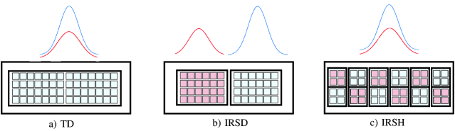
Figure 3: Illustration of three protocols for sharing the IRS between two LSs emitting Gaussian beams. The blue and red colors indicate the LS beams and the tiles allocated to the different LS-PD pairs.

IV-A IRS Sharing Protocols

IV-A1 TD Protocol

For the TD protocol, in each time slot, one LS transmits, while the other LSs are inactive, thus, the number of time slots, $T$, is identical to the number of FSO links, $N$, i.e., $T=N$. In each time slot, the entire IRS surface is configured for the active LS-PD pair, i.e., only one tile is needed and $Q=1$, see Fig. 3a). Moreover, in order to maximize the received power, the phase shift profile center, the incident beam footprint center, and the lens center on the IRS should coincide with the origin, i.e., $\mathbf{r}_{q}^{t}=\mathbf{r}_{\ell 0,m}=\mathbf{r}_{p0,n}=(0,0,0),\,\forall m,n\in\mathcal{N}$. For this protocol, the active PD receives maximum power as the IRS serves only one LS-PD pair at a time. However, the time sharing among LSs degrades the achievable data rate.

IV-A2 IRSD Protocol

For this protocol, all LSs simultaneously illuminate the IRS, which is divided into $Q=N$ tiles, see Fig. 3b). We assume that each LS-PD pair is assigned to a different tile such that the centers of the beam footprints, the lens centers, and the tile phase shift profile centers coincide with the centers of the respective tiles, i.e., $\mathbf{r}_{\ell 0,m}=\mathbf{r}_{p0,n}=\mathbf{r}_{q}^{t}=\mathbf{r}_{q},\forall m,n\in\mathcal{N}$. Since all LSs transmit simultaneously, the data rate may be increased compared to the TD protocol. However, due to the partitioning of the IRS among multiple FSO links, unless the IRS is sufficiently large, only part of the incident power is reflected by the respective tile towards the desired lens. Thereby, the larger the incident beamwidth, the less power is received at the lens. Moreover, misalignment errors may shift the beam footprint center or the lens center on the IRS towards a tile reserved for a different LS-PD pair. Thus, given the Gaussian beam intensity distribution, a portion of the power may be redirected in an undesired direction which in turn degrades the GML.

IV-A3 IRSH Protocol

Since perfect tracking of the tile, beam footprint, and lens centers may not always be feasible, we propose the homogenization of the IRS surface by dividing it into $Q$ tiles such that the number of tiles is much larger than the number of LS-PD pairs, i.e., $Q\gg N$, see Fig. 3c). Unlike for the IRSD protocol, where one tile is assigned to one LS-PD pair, for this protocol, multiple smaller tiles are allocated to each LS-PD pair, and thus, the LS beam power is distributed across multiple tiles. Thus, if the beam footprint center or/and the lens center on the IRS are shifted due to misalignment errors, the impact on the receive power will be mitigated. This benefit comes at the cost of a power loss since only some of the tiles around beam center are designed to redirect the beam towards the desired lens. Thereby, the IRSH protocol is more resilient to misalignment errors, but without misalignment, the IRSD and TD protocols may achieve a higher performance as they redirect more power to the desired lenses.

IV-B Tile Configuration

For all proposed IRS sharing protocols, at a given time, each tile is assigned to only one LS-PD pair. In the following, we determine the phase shift profile of the $q$-th tile, $\Phi_{q}(\mathbf{r},\mathbf{r}_{q}^{t})$, needed to redirect the LS beam towards a desired PD and the corresponding efficiency factor, $\zeta_{q}$, required for a passive-lossless IRS.

IV-B1 Tile Phase Shift Profile $\Phi_{q}(\mathbf{r},\mathbf{r}_{q}^{t})$

The phase shift introduced by the tile is exploited such that it compensates the phase difference between the incident and the desired beam. Moreover, the incident beam on the IRS has a nonlinear phase profile (8) and the phase profile of the secondary waves (9) include linear or quadratic terms depending on the operating regime and the approximation used, cf. Section III-C. Thus, the desired phase shift across the tile is in general a nonlinear function. Assuming that the positions of the $m$-th LS, $\left(d_{\ell m},\mathbf{\Psi}_{\ell m}\right)$, and the $n$-th PD, $\left(d_{pn},\mathbf{\Psi}_{pn}\right)$, are known, we adopt LP and QP profiles as approximations of general nonlinear phase shift profiles as follows

$$\Phi_{q}^{\text{quad}}(\mathbf{r},\mathbf{r}_{q}^{t}) =k\left(\Phi_{q,0}+\Phi_{q,x}(x-x_{q}^{t})+\Phi_{q,y}(y-y_{q}^{t})+\Phi_{q,x^{2}}(x-x_{q}^{t})^{2}+\Phi_{q,y^{2}}(y-y_{q}^{t})^{2}\right),\qquad$$ (22a)

$$\Phi_{q}^{\text{lin}}(\mathbf{r},\mathbf{r}_{q}^{t}) =k\left(\Phi_{q,0}+\Phi_{q,x}(x-x_{q}^{t})+\Phi_{q,y}(y-y_{q}^{t})\right),\qquad$$ (23a)

where $\Phi_{q,x}=\cos(\theta_{\ell m})\cos(\phi_{\ell m})+\cos(\theta_{pn})\cos(\phi_{pn})$, $\Phi_{q,y}=\cos(\theta_{\ell m})\sin(\phi_{\ell m})+\cos(\theta_{pn})\sin(\phi_{pn})$, $\Phi_{{q,x^{2}}}=\frac{1}{2d_{pn}}\left(1+\cos^{2}(\theta_{pn})\cos^{2}(\phi_{pn})\right)-\frac{\sin^{2}(\theta_{\ell m})}{2R(\hat{d}_{\ell m})}-\frac{1}{4d_{pn}}$, $\Phi_{q,y^{2}}\!=\frac{1}{2d_{pn}}\big{(}1\!+\cos^{2}(\theta_{pn})\sin^{2}(\phi_{pn})\big{)}-\frac{1}{2R(\hat{d}_{\ell m})}-\frac{1}{4d_{pn}}$, and $\Phi_{q,0}=d_{pn}-\hat{d}_{\ell m}$. The LP profile is chosen such that the total accumulated phase, see (39), is zero when the beam arrives at the lens center. Then, for the QP profile, the quadratic terms cancel the total accumulated phase due to the LS beam curvature and the IRS-to-lens distance. Furthermore, adding the term $-\frac{1}{4d_{pn}}$ causes a parabolic phase profile that focuses the beam at the lens center. These phase profiles allow the application of Theorems 1 and 2. Moreover, the LP profile in (23a) corresponds to the generalized Snell’s law given in [26, 7].

IV-B2 Tile Efficiency $\zeta_{q}$

The efficiency factor $\zeta_{q}$ ensures that the power reflected from the tile is smaller or equal to the power incident on the tile. We assume $\zeta_{q}=\zeta_{0}\bar{\zeta}_{q}$, where $\zeta_{0}$ denotes the resistive loss of the IRS and $\bar{\zeta}_{q}$ is the passivity constant which ensures the incident power is completely reflected.

Proposition 1

The passivity factor $\bar{\zeta}_{q}$ of tile $q$ which is assigned to the $m$-th LS and the $n$-th lens depends on $\mathbf{\Psi}_{pn}$ and is given by

$$\bar{\zeta}_{q}=\sqrt{\lvert\sin(\theta_{pn})\rvert}.$$ (24)

Proof:

The proof is given in Appendix D. ∎

In particular, using the above result for anomalous reflection in the far-field scenario in (18), we obtain ${\zeta}_{t}^{2}=\frac{\lvert\sin(\theta_{pn})\rvert}{\lvert\sin(\theta_{\ell m})\rvert}$, which is similar to the result for plane waves given in [17, 16].

V Performance Analysis

For the IRSD and IRSH protocols, the IRS surface is shared by multiple links. Hence, in principle, inter-link interference can affect the end-to-end performance. However, by careful positioning of the LSs and PDs, inter-link interference can be considerably mitigated. Nevertheless, in the following, we analyze the end-to-end performance of the considered IRS-assisted multi-link FSO transmission systems taking into account the possibility of inter-link interference.

V-A Bit Error Rate

To analyze the average BER for the $n$-th LS-PD pair, we first derive the instantaneous BER for a given realization of the atmospheric turbulence induced fading in the presence of interference in the following Lemma.

Lemma 2

Assuming OOK modulated symbols $s_{m}$ with signal power $P_{\ell m},m\in\mathcal{N}$, and AWGN noise $w_{n}\sim\mathcal{N}(0,\sigma_{w}^{2})$, an error occurs if symbol $\hat{s}_{n}\neq s_{n}$ is detected by the $n$-th PD. The corresponding BER is given by

$$P_{e,n}(\mathbf{h}_{a}^{n}) =\frac{1}{2^{N}}\sum_{\mathbf{s}_{m}\in\mathcal{S}_{m}}Q\left(\frac{1}{2}h_{a}^{n,n}\sqrt{\gamma_{n}}-\!\sum_{\begin{subarray}{c}m\in\mathcal{N}\\ m\neq n\end{subarray}}h_{a}^{m,n}s_{m}\sqrt{\gamma_{m}}\right)$$ (25)

$$+\frac{1}{2^{N}}\sum_{\mathbf{s}_{m}\in\mathcal{S}_{m}}Q\left(\frac{1}{2}h_{a}^{n,n}\sqrt{\gamma_{n}}+\!\sum_{\begin{subarray}{c}m\in\mathcal{N}\\ m\neq n\end{subarray}}h_{a}^{m,n}s_{m}\sqrt{\gamma_{m}}\right),$$

where $\mathbf{h}_{a}^{n}=[h_{a}^{1,n},\dots,h_{a}^{N,n}]$, $\mathbf{s}_{m}=[s_{1},\dots,s_{n-1},s_{n+1},\dots,s_{N}]$ denotes the vector of interfering symbols $s_{m}$, $\mathcal{S}_{m}=\{0,1\}^{N-1}$, $\gamma_{\iota}=\frac{P_{\ell\iota}}{\sigma_{w}^{2}}|h_{\text{irs}}^{\iota,n}h_{p}^{\iota,n}|^{2},\iota\in\{n,m\}$, and $Q(\cdot)$ is the Gaussian Q-function.

Proof:

The proof is given in Appendix E. ∎

Then, given that $h_{a}^{m,n},\forall m\in\mathcal{N},$ are independent random variables, the average BER for the $n$-th LS-PD pair, denoted by $P_{e,n}$, is given by

$$P_{e,n}=\int_{0}^{\infty}\dots\int_{0}^{\infty}P_{e,n}(\mathbf{h}_{a}^{n})f_{h_{a}^{1,n}}(h_{a}^{1,n})\dots f_{h_{a}^{N,n}}(h_{a}^{N,n})\mathrm{d}\mathbf{h}_{a}^{n},$$ (26)

where $f_{h_{a}^{m,n}}(\cdot)$ is the probability density function (PDF) of a Gamma-Gamma distributed random variable which is given by [27]

$$f_{h_{a}^{m,n}}(h_{a}^{m,n})=\frac{2(\alpha_{m,n}\beta_{m,n}h_{a}^{m,n})^{\frac{\alpha_{m,n}+\beta_{m,n}}{2}}}{\Gamma(\alpha_{m,n})\Gamma(\beta_{m,n})h_{a}^{m,n}}K_{\alpha_{m,n}-\beta_{m,n}}\left(2\sqrt{{\alpha_{m,n}\beta_{m,n}}h_{a}^{m,n}}\right),$$ (27)

where $\Gamma(\cdot)$ is the Gamma function, and $K_{v}(\cdot)$ is the modified Bessel function of the second kind with order $v$. Eq. (26) involves an $N$ dimensional integral which can be evaluated numerically, especially if $N$ is small, e.g., for $N=2$ LS-PD pairs, as considered in Section VI for our numerical results. For large $N$, (26) can be approximated using the PDF of the sum of Gamma-Gamma distributed variables in [27, Eqs. (24) and (25)].

For the special case of noise limited systems, where the inter-link interference in (25) can be ignored, we obtain $P_{e,n}=P_{e}\left(\sqrt{\frac{\gamma_{n}}{4}}\right)$ [28], where $P_{e}(x)$ is given by

$$P_{e}(x)= \sum_{\iota=0}^{\infty}\left(\xi_{\iota}(\alpha_{n,n},\beta_{n,n})(4x)^{-{\iota+\beta_{n,n}\over 2}}+\xi_{\iota}(\beta_{n,n},\alpha_{n,n})(4x)^{-{\iota+\alpha_{n,n}\over 2}}\right),$$ (28)

and

$$\xi_{\iota}(\alpha_{n,n},\beta_{n,n})={\sqrt{\pi}(2\sqrt{2}\alpha_{n,n}\beta_{n,n})^{\iota+\beta_{n,n}}{\Gamma}\left({\iota+\beta_{n,n}+1\over 2}\right)\over 2\sin[\pi(\alpha_{n,n}-\beta_{n,n})]\Gamma(\alpha_{n,n})\Gamma(\beta_{n,n})\Gamma(\iota-\alpha_{n,n}+\beta_{n,n}+1)(\iota+\beta_{n,n})\iota!}.\qquad$$ (29)

V-B Outage Probability

Given the high data rates of FSO systems (10 $\text{Gbit}/\text{s}$) compared to the coherence time of the channel (1-10 ms) and in order to investigate the trade-off between the transmission rate and the received power of the proposed IRS protocols, we study the outage probability. The outage probability of the $n$-th LS-PD pair is defined as the probability that the fixed data rate of the LS, $R_{n}$, exceeds the capacity of the end-to-end channel, $\mathcal{C}_{n}$, and is given by

$$P_{\text{out},n}=\text{Pr}\{\mathcal{C}_{n}<R_{n}\}.$$ (30)

To evaluate (30), first we provide a lower bound for the capacity of the FSO interference channel in the following lemma.

Lemma 3

Assuming $s_{n}[t]\in\mathbb{R}^{+}$ with an average power constraint, $\mathbb{E}\{|s_{n}[t]|^{2}\}\leq P_{\ell n}$, and Gaussian noise $w_{n}[t]$ with variance $\sigma_{w}^{2}$, the capacity of the interference channel in (1) is lower bounded by

$$\mathcal{C}_{n}\geq\mathcal{C}_{\text{low}}(\Upsilon_{n}),$$ (31)

where $\mathcal{C}_{\text{low}}(\Upsilon_{n})=\frac{W_{\text{FSO}}}{2}\ln\left(1+\frac{\Upsilon_{n}e}{2\pi}\right)$, $\Upsilon_{n}=\frac{|h_{n,n}|^{2}P_{\ell n}}{\tilde{\sigma}_{s}^{2}+\sigma_{{w}}^{2}}$, and $\tilde{\sigma}_{s}^{2}=\sum\limits_{\begin{subarray}{c}m=1\\ m\neq n\end{subarray}}^{N}P_{\ell m}|h_{m,n}|^{2}$.

Proof:

The proof is given in Appendix F. ∎

Using the above lemma and (30), we obtain an upper bound on the outage probability in (30) as follows

$$P_{\text{out},n}\leq P_{\text{out},n}^{\text{up}}=\text{Pr}\{\mathcal{C}_{\text{low}}(\Upsilon_{n})<R_{n}\}\overset{(a)}{=}\text{Pr}\{\Upsilon_{n}<\gamma_{\text{thr}}\},$$ (32)

where for $(a)$, we exploit that $\mathcal{C}_{\text{low}}(\cdot)$ is a monotonically increasing function in $\Upsilon_{n}$, and thus, an outage occurs when the received SINR falls below threshold $\gamma_{\text{thr}}=\mathcal{C}_{\text{low}}^{-1}\left(R_{n}\right)=\frac{2\pi}{e}\left(e^{2R_{n}/W_{\text{FSO}}}-1\right)$. Next, given the randomness of the turbulence induced fading, $h_{a}^{m,n}$, $P_{\text{out},n}^{\text{up}}$ is given by

$$P_{\text{out},n}^{\text{up}}=\text{Pr}\{\Upsilon_{n}<\gamma_{\text{thr}}\}=\text{Pr}\left\{\left(h_{a}^{n,n}\right)^{2}<\bar{\chi}\right\}=$$

$$\int_{0}^{\infty}\dots\int_{0}^{\infty}F_{h_{a}^{n,n}}\left(\sqrt{\bar{\chi}}\right)f_{h_{a}^{1,n}}(h_{a}^{1,n})\dots f_{h_{a}^{n-1,n}}(h_{a}^{n-1,n})f_{h_{a}^{n+1,n}}(h_{a}^{n+1,n})\dots f_{h_{a}^{N,n}}(h_{a}^{N,n})\mathrm{d}\bar{\mathbf{h}}_{a}^{n},\qquad$$ (33)

where $\bar{\mathbf{h}}_{a}^{n}=[h_{a}^{1,n},\dots,h_{a}^{n-1,n},h_{a}^{n+1,n},\dots h_{a}^{N,n}]$, $\bar{\chi}={\gamma_{\text{thr}}\over\gamma_{n}}\sum\limits_{\begin{subarray}{c}m=1\\ m\neq n\end{subarray}}^{N}\gamma_{m}|h_{a}^{m,n}|^{2}+{\gamma_{\text{thr}}\over\gamma_{n}}$, and $F_{h_{a}^{n,n}}(\cdot)$ denotes the cumulative distribution function (CDF) of the Gamma-Gamma distribution given in [29, Eq. (7)]. For small $N$, the above equation can be numerically integrated. For large $N$, (33) can be approximated using the PDF of the sum of squared Gamma-Gamma distributed variables given in [30, Eq. (9)].

As a special case, for noise limited systems, where the impact of inter-link interference can be ignored, the upper bound on the outage probability can be simplified as follows

$$P_{\text{out},n}^{\text{up}}=\text{Pr}\{\left(h_{a}^{n,n}\right)^{2}\leq\Upsilon_{\text{thr}}\}=F_{h_{a}^{n,n}}\left(\sqrt{\Upsilon_{\text{thr}}}\right),$$ (34)

where $\Upsilon_{\text{thr}}=\frac{\gamma_{\text{thr}}}{\gamma_{n}}$. Substituting $F_{h_{a}^{n,n}}(\cdot)$ given in [29, Eq. (7)] in (34), the upper bound on the outage probability is given by [31]

$$P_{\text{out},n}^{\text{up}}={1\over\Gamma(\alpha_{n,n})\Gamma(\beta_{n,n})}\,G_{1,3}^{2,1}\left[\alpha_{n,n}\beta_{n,n}\sqrt{\Upsilon_{\text{thr}}}\bigg{|}_{\alpha_{n,n},\beta_{n,n},0}^{1}\right],$$ (35)

where $G_{m,n}^{p,q}\left[x\bigg{|}_{b_{1},\cdots,b_{q}}^{a_{1},\cdots,a_{p}}\right]$ is the Meijer’s G-function.

VI Simulation Results

TABLE I: System and channel parameters [1], [7].

LS Parameters	Symbol	Value
FSO bandwidth	$W_{\text{FSO}}$	$1\ \mathrm{GHz}$
FSO wavelength	$\lambda$	$1550\,\mathrm{nm}$
Beam waist radius	$w_{01},w_{02}$	$0.25\ \mathrm{mm}$
Electric fields at origin	$E_{01},E_{02}$	$60\,\frac{\mathrm{kV}}{\mathrm{m}}$
Noise spectral density	$N_{0}$	$-114\ \mathrm{dBm}/\mathrm{MHz}$
Attenuation coefficient	$\kappa$	$0.43\times 10^{-3}\frac{\mathrm{dB}}{\mathrm{m}}$
Distance and orientation of LS 1	$d_{\ell 1},\mathbf{\Psi}_{\ell 1}$	$1\,\text{km},\left({\pi\over 3},0\right)$
Distance and orientation of LS 2	$d_{\ell 2},\mathbf{\Psi}_{\ell 2}$	$1\,\text{km},\left({\pi\over 4},0\right)$
Gamma-Gamma parameters	$(\alpha,\beta)$	$(2,2)$
Impedance of the propagation medium	$\eta$	$377\,\Omega$
IRS Parameters
IRS Size	$L_{x,\text{tot}}\times L_{y,\text{tot}}$	$1$ m $\times 0.5$ m
Separation distance between tiles	$l_{x},l_{y}$	$0,0$
Number of tiles for TD protocol	$Q_{x}\times Q_{y}$	$1\times 1$
Number of tiles for IRSD protocol	$Q_{x}\times Q_{y}$	$2\times 1$
Number of tiles for IRSH protocol	$Q_{x}\times Q_{y}$	$8\times 2$
PD and Lens Parameters
Lenses radius	$a$	$15\ \mathrm{cm}$
Distance and orientation of lens of PD 1	$d_{p1},\mathbf{\Psi}_{p1}$	$3\,\text{km},\left({\pi\over 3},\pi\right)$
Distance and orientation of lens of PD 2	$d_{p2},\mathbf{\Psi}_{p2}$	$3\,\text{km},\left({\pi\over 6},\pi\right)$

In this section, first we validate the analytical channel gain in (20) for a point-to-point IRS-assisted FSO link. Then, we consider the case where two LS-PD pairs share one IRS, see Fig. 5, and determine the impact of inter-link interference. Finally, we investigate the system performance in terms of BER and outage probability. The LP profile across the IRS in (23a) is applied except for Fig. 7, where also the QP profile in (22a) is considered. For all figures, the parameter values provided in Table I are adopted, unless specified otherwise.

VI-A Validation of the Channel Model

First, we validate our analytical results for the point-to-point GML for the IRS-assisted FSO system in (20). For Fig. 5, we assume that LS 1 is connected via a single-tile IRS to PD 1. Fig. 5 shows the analytical GML, $h_{\text{irs}}^{1,1}$, in (20), the numerical integration of the Huygens-Fresnel integral using (9), (4), and (3), and the GML obtained with the far-field approximation in (18), where an IRS size of $L_{x,\text{tot}}=L_{y,\text{tot}}=0.5$ m is assumed. As can be observed, for larger IRS-lens distances, the GML decreases which is due to the divergence of the laser beam along the propagation path. Thus, for large distances, the lens receives a smaller portion of the LS beam power which leads to a smaller GML. Fig. 5 also shows that the proposed analytical GML in (20) matches the Huygens-Fresnel results for both IRS sizes, whereas the far-field approximation in (18) is only valid in the far-field regime. The subfigure in Fig. 5 shows the far-field regime. The mismatch between the GML for the far-field approximation and the Huygens-Fresnel results can be explained based on the definition of the far-field distance in (13). Here, the LS beam width incident on the IRS is $w_{x}(\hat{d}_{\ell 1})=2.28$ m and $w_{y}(\hat{d}_{\ell 1})=1.97$ m. From (13), we obtain the minimum far-field distance as $d_{f}=40.3$ km. At distances $d_{p1}>d_{f}$, the analytical GML and the Huygens-Fresnel results approach the far-field approximation. Fig. 5 confirms that for the typical range of FSO systems of a few kilometers, the proposed analytical channel model is valid for practical IRS sizes and IRS-lens distances, whereas the far-field approximation does not always yield accurate results.

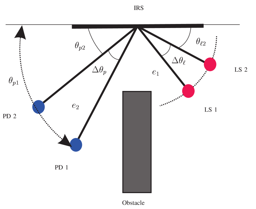
Figure 4: Simulation setup.

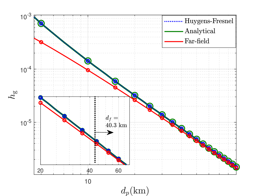
Figure 5: GML for IRS-based FSO channel between LS 1 and PD 1 versus $d_{p1}$.

VI-B Interference Channel Power

In the following, we consider a rectangular-shaped IRS of size $L_{x,\text{tot}}=1$ m and $L_{y,\text{tot}}=0.5$ m. Two LS-PD pairs are connected via the IRS, see Fig. 5 . The LSs and lenses are located on circles centered at the origin and with radii $e_{1}=1$ km and $e_{2}=3$ km, respectively. LS 2 and PD 2 are fixed at angles $\mathbf{\Psi}_{\ell 2}=({\pi\over 4},0)$ and $\mathbf{\Psi}_{p2}=({\pi\over 6},\pi)$, respectively. LS 1 and PD 1 are located at angles $\mathbf{\Psi}_{\ell 1}=({\pi\over 4}+\Delta\theta_{\ell},0)$ and $\mathbf{\Psi}_{p1}=(\theta_{p1}={\pi\over 6}+\Delta\theta_{p},\pi)$, respectively, i.e., the two LSs and the two PDs are separated by angles $\Delta\theta_{\ell}$ and $\Delta\theta_{p}$, respectively. The IRS employs the TD, IRSD, and IRSH protocols to allow both LS-PD pairs to share its surface. PD 1 receives the reflected signal of the desired transmitter LS 1 and for the IRSD and IRSH protocols, that of the interfering transmitter LS 2. Fig. 6 shows the signal power, $\gamma_{1}$, and the interference power, $\gamma_{2}$, received at PD 1 as a function of angle $\theta_{p1}$. Results for LS separation angles $\Delta\theta_{\ell}=0$ mrad and 1 mrad are shown in Figs. 6(a) and 6(b), respectively. As can be observed, by increasing $\theta_{p1}$, both the received signal power and the interference power increase since the LS power captured by the lens plane is maximized when it is parallel to the IRS plane. Moreover, Figs. 6(a) and 6(b) reveal that the TD and IRSD protocols capture the same amount of signal power since for both protocols the respective IRS tile is smaller than the beam footprint in the IRS plane. Furthermore, for the TD and IRSD protocols, the beam axis of LS 1 and the lens center on the IRS coincide with the center of the tile configured for LS 1 and PD 1, whereas the IRSH protocol disregards the positioning of the beam axis and lens centers on the tile. Thus, PD 1 can collect more power for the TD and IRSD protocols than for the IRSH protocol. Moreover, for the IRSD protocol, the interference power for both values of $\Delta\theta_{\ell}$ is considerably smaller than the signal power since the two LS beams and the two lens centers are assigned to the centers of different IRS tiles. For the IRSH protocol, the interference power and the signal power are similar when the LSs are co-located ($\Delta\theta_{\ell}=0$ mrad), see Fig. 6(a), whereas after slightly increasing the separation angle between the LSs to $\Delta\theta_{\ell}=1$ mrad in Fig. 6(b), the IRSH protocol yields a similar interference power as the IRSD protocol. In summary, for the IRSD and IRSH protocols, the interference can be limited by suitable positioning of the beam footprints and the lens centers on the IRS and by careful positioning of the LSs and PDs, respectively.

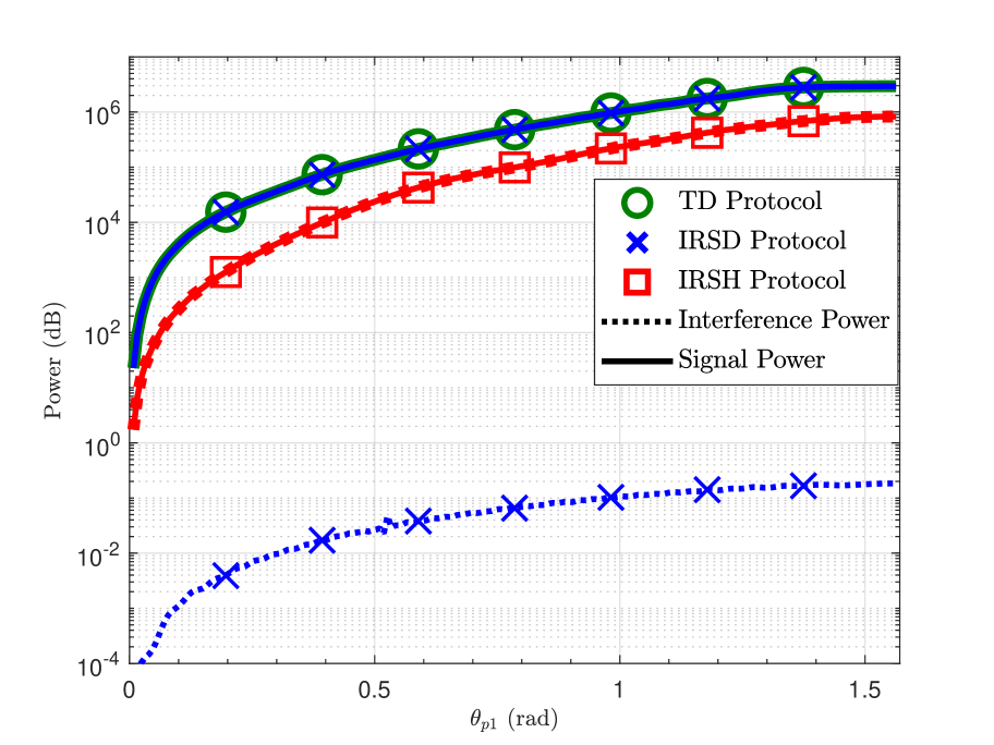
(a)

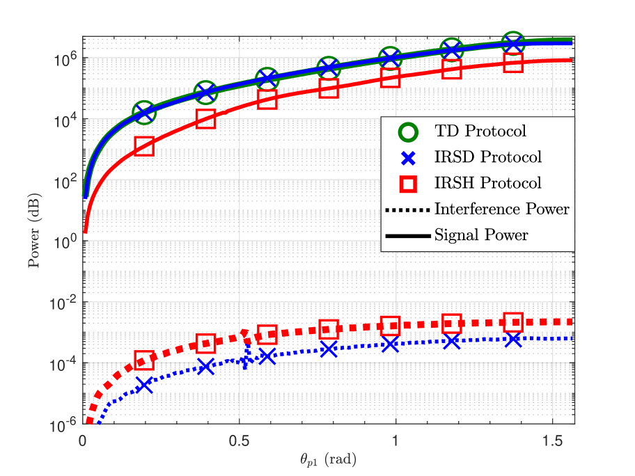
(b)

Figure 6: The power of the desired signal from LS 1 at PD 1 and the interference signal from LS 2 at PD 1. The figure shows the power versus $\theta_{p1}$ for two setups (a) $\Delta\theta_{\ell}=0$ rad and (b) $\Delta\theta_{\ell}=1$ mrad.

VI-C Performance Analysis

In the following, we investigate the performance of the setup specified in Fig. 5 and Table I in terms of BER and outage probability. The simulation results are averaged over $10^{6}$ channel realizations.

Fig. 7 shows simulation and analytical results (26) for the BER of the LS 1-PD 1 link for different IRS sharing protocols employing the LP and QP profiles given in (23a) and (22a), respectively. Figs. 8(a) and 8(b) show the BER for co-located LSs and separated LSs with $\Delta\theta_{\ell}=1$ mrad, respectively. In both subfigures, the simulation results and analytical results (26) match perfectly. The TD and IRSD protocols achieve a lower BER than the IRSH protocol. This can be explained as follows. For the considered protocols, the beam of LS 1 incident on the IRS has beamwidths $w_{x}(\hat{d}_{\ell 1})=2.28$ m and $w_{y}(\hat{d}_{\ell 1})=1.97$ m. The tile sizes for the IRSD and IRSH protocols are $L_{x}=L_{y}=0.5$ m and $L_{x}=0.125$ m, $L_{y}=0.5$ m, respectively, whereas the TD protocol allocates the entire IRS surface to one LS-PD pair. As we observed in Figs. 6(a) and 6(b), for the TD and IRSD protocols, the lens can collect more power than for the IRSH protocol which leads to a better BER performance in Figs. 8(a) and 8(b). Furthermore, in Fig. 8(a), we observe a large BER degradation for the IRSH protocol. This is due to the interference caused by LS 2 at PD 1 when the LSs are co-located, see Fig. 6(a). This unfavorable behavior can be easily mitigated by separating the LSs by 1 mrad as shown in Fig. 8(b). Furthermore, we observe that the QP design achieves a substantial gain of up to 12 dB over the LP design for all considered protocols. The QP design in (22a) reduces the beam divergence along the propagation path which in turn increases the received power at the lens. Moreover, the TD protocol yields a 2 dB gain over the IRSD protocol for the QP profile, whereas both protocols perform similarly for the LP profile. For the LP profile, the beam diverges and since the lens is smaller than the beam footprint in the lens plane, the performances of both protocols are similar. On the other hand, for the QP profile, the larger IRS tile for the TD protocol allows focusing more power on the lens, which leads to a better BER performance.

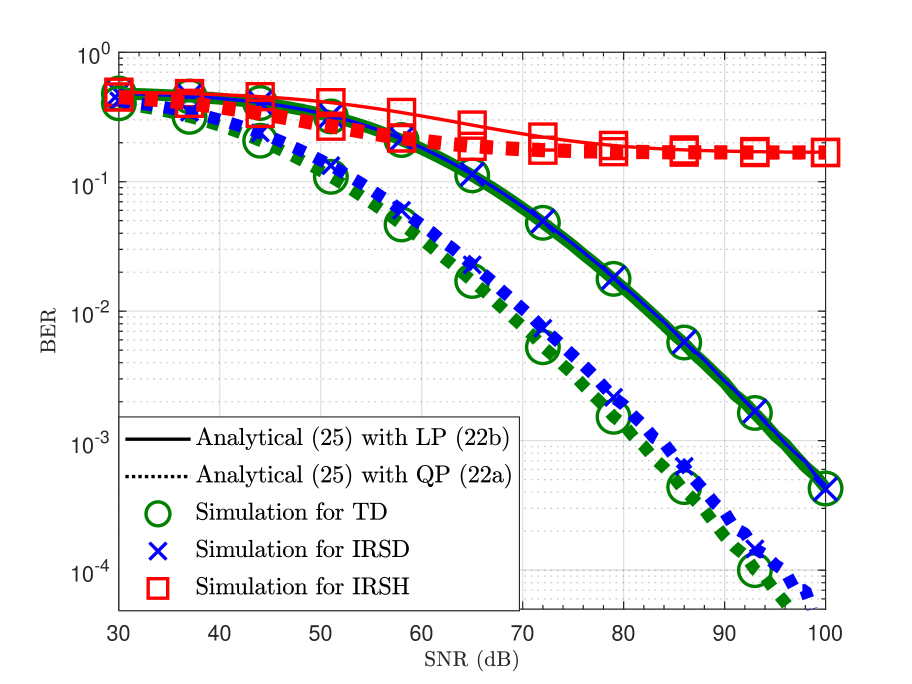
(a)

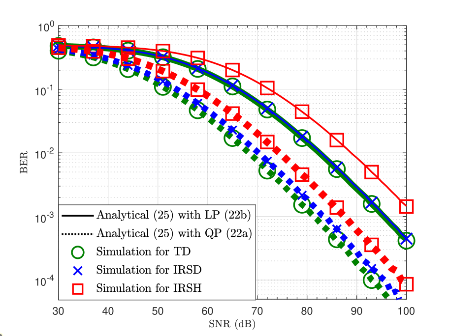
(b)

Figure 7: BER performance versus SNR (dB) with LP and QP profiles for three IRS sharing protocols, where $\theta_{p1}=\frac{\pi}{3}$, $\theta_{p2}=\frac{\pi}{6}$, and (a) $\Delta\theta_{\ell}=0$ rad and (b) $\Delta\theta_{\ell}=1$ mrad.

Figs. LABEL:Fig:Outage1 and LABEL:Fig:Outage2 show the upper bounds on the outage probability of the link between LS 1 and PD 1 for threshold rates $R_{1}=1.7$ $\mathrm{Gbit}/\mathrm{s}$ and $0.5$ $\mathrm{Gbit}/\mathrm{s}$, respectively. The performances of the three IRS sharing protocols are compared for misalignment errors $|\mathbf{r}_{\ell 1}-\mathbf{r}_{p1}|=0$ m and $0.17$ m. The LS locations are as specified in Table I. In both subfigures, the simulation results perfectly match the analytical results in (33). Moreover, by increasing angle $\theta_{p1}$, the IRS and lens become more parallel to each other which leads to a larger received power at PD 1 and a lower outage probability. For both threshold rates, in the absence of misalignment errors, the IRSD protocol performs better than the IRSH and TD protocols because of the larger received power at the lens and the simultaneous transmission of both LSs, respectively. Furthermore, for the larger threshold rate, i.e., $R_{1}=1.7$ $\mathrm{Gbit}/\mathrm{s}$, considered in Fig. LABEL:Fig:Outage1 the IRSH protocol performs better than the TD protocol. This is expected since for the TD protocol, LS 1 can transmit only in half of the time slots. However, for the smaller threshold rate, i.e., $R_{1}=0.5$ $\mathrm{Gbit}/\mathrm{s}$, considered in Fig. LABEL:Fig:Outage2, the TD protocol performs better than the IRSH protocol because the benefit of a larger received power outweighs the rate loss associated with the TD protocol in this case. Moreover, for both considered threshold rates, the performance of the IRSD protocol degrades significantly for a misalignment error of $0.17$ m. This is due to the shift of the beam of LS 1 incident on the IRS towards the tile that is configured for LS 2. This tile redirects the power of LS 1 in the wrong direction. In contrast, the IRSH protocol is robust to misalignment errors, due to the homogenization of the IRS.

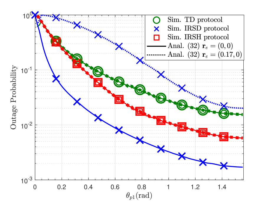
(a)

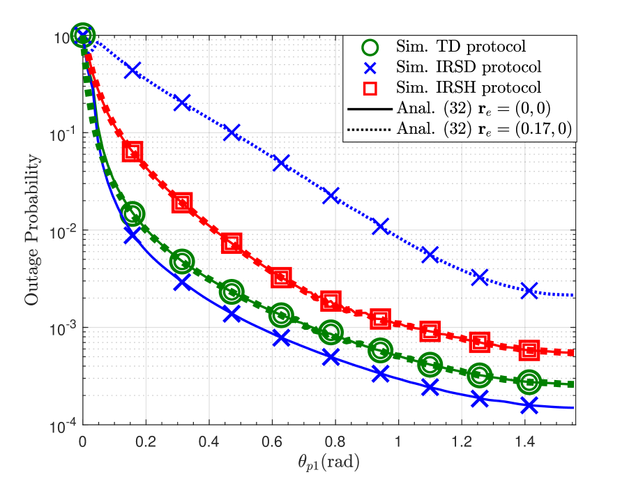
(b)

Figure 8: Upper bounds on the outage probability versus $\theta_{p1}$ (rad) for misalignment errors $|\mathbf{r}_{e}|=|\mathbf{r}_{\ell 1}-\mathbf{r}_{p1}|=0$ m and $0.17$ m and threshold rates (a) $R_{1}=1.7$ $\mathrm{Gbit}/\mathrm{s}$ and (b) $R_{1}=0.5$ $\mathrm{Gbit}/\mathrm{s}$.

VII Conclusions

In this paper, we developed an analytical channel model for point-to-point IRS-assisted FSO systems based on the Huygens-Fresnel principle. We determined the reflected electric field and the channel gain taking into account the non-uniform power distribution of Gaussian beams, the IRS size, the positions of the LS, the IRS, and the lens, and the phase shift profile of the IRS. We validated the accuracy of the proposed analytical model via simulations and showed that, in contrast to models based on the far-field approximation, the proposed model is valid even for intermediate distances, which are relevant in practice. Moreover, we exploited the proposed model to study the performance of an IRS-assisted multi-link FSO system, where we proposed three IRS sharing protocols. For each protocol, we designed the size and phase shift profile of the IRS tiles, the position of the beam footprint, and the lens w.r.t. the IRS. Then, we analyzed the BER and outage probability and exploited this analysis to compare the IRS sharing protocols in the presence of misalignment errors and inter-link interference and for LP/QP profiles. Our results revealed that the impact of interference can be mitigated by careful positioning of the LSs and PDs. Moreover, the QP profile was shown to outperform the LP profile. Furthermore, which of the proposed IRS sharing protocols is preferable, depends on the position of the LSs and PDs, the target transmission rate, and on whether or not misalignment errors are present.

Appendix A Proof of Lemma 1

First, we express the LS plane coordinates $\mathbf{r}_{l}$ in terms of the Cartesian coordinates $\mathbf{r}$ as follows

$${\mathbf{r}}_{l}=\mathbf{R}^{T}_{y_{l}}\left({\frac{\pi}{2}}-\theta_{l}\right)\left({\mathbf{r}}-{\mathbf{r}}_{\ell 0}\right)+\mathbf{c}_{1},$$ (36)

where $\mathbf{c}_{1}=(0,0,d_{l})$, $\mathbf{R}_{y_{l}}(\cdot)$ is a rotation matrix, and ${z}=0$ since the tile plane is located in the $xy$-plane. Then, assuming $d_{l}\gg L_{x},L_{y}$, we can approximate ${z}_{l}\approx\hat{d}_{l}$ in the terms ${w}^{2}(\cdot)$, $R(\cdot)$, and $\tan^{-1}\left(\cdot\right)$ in (6). Then, by substituting these variables in (6), we obtain (8). Then, because of the law of energy conservation [32], the LS beam power and the power collected by an IRS with infinitely large area, i.e., $L_{x},L_{y}\to\infty$, must be the same. Thus, using (4) and (3), we obtain

$$\frac{1}{2\eta}\int\limits_{-\infty}^{\infty}\int\limits_{-\infty}^{\infty}|E_{\ell}(\mathbf{r}_{\ell})|^{2}\mathrm{d}{x}_{\ell}\mathrm{d}{y}_{\ell}=\frac{1}{2\eta}\int\limits_{-\infty}^{\infty}\int\limits_{-\infty}^{\infty}|{E}_{\text{in}}({\mathbf{r}})|^{2}\mathrm{d}x\mathrm{d}y.$$ (37)

Thus, using [23, Eq. 3.321-2], we obtain $\zeta_{\text{in}}=\sqrt{\sin(\theta_{\ell})}$ and this completes the proof.

Appendix B Proof of Theorem 1

First, we substitute (8) and $\Phi_{q}(\mathbf{r},\mathbf{r}_{q}^{t})=\Phi_{q}^{\text{quad}}(\mathbf{r},\mathbf{r}_{q}^{t})$ into (9) and approximate $|\mathbf{r}_{o}-{\mathbf{r}}|\approx\text{t}_{1}+\text{t}_{2}$, see (11). This leads to

$$E_{q}(\mathbf{r}_{o}) =\int_{-\frac{L_{y}}{2}+y_{q}}^{\frac{L_{y}}{2}+y_{q}}\!\!\int_{-\frac{L_{x}}{2}+x_{q}}^{\frac{L_{x}}{2}+x_{q}}A({x},{y})\exp\left(j\Phi_{\text{tot}}({x},{y})\right)\mathrm{d}{x}\mathrm{d}{y},$$ (38)

where amplitude $A({x},{y})=\frac{E_{0}w_{0}\zeta_{q}}{\lambda{w}(\hat{d}_{\ell})|\mathbf{r}_{o}-{\mathbf{r}}|}\exp\left(-{\hat{x}^{2}\over{w}_{x}^{2}(\hat{d}_{\ell})}-{{\hat{y}}^{2}\over{w}_{y}^{2}(\hat{d}_{\ell})}\right)$ and the total phase is the summation of the incident beam phase, $\psi_{\text{in}}({\mathbf{r}})$, the quadratic phase shift of the tile, $\Phi_{q}^{\text{quad}}(\mathbf{r},\mathbf{r}_{q}^{t})$, and the additional phase from the IRS to the lens, $k|\mathbf{r}_{o}-{\mathbf{r}}|$, and is given by

$$\Phi_{\text{tot}}({\mathbf{r}}) =-\psi_{\text{in}}({\mathbf{r}})+k|\mathbf{r}_{o}-{\mathbf{r}}|-\Phi_{q}^{\text{quad}}(\mathbf{r},\mathbf{r}_{q}^{t}),$$ (39)

where $\psi_{\text{in}}({\mathbf{r}})$ and $|\mathbf{r}_{o}-{\mathbf{r}}|$ are respectively given by (8) and approximated by terms $\text{t}_{1}$ and $\text{t}_{2}$ in (11). Thus, by further approximating $|\mathbf{r}_{o}-{\mathbf{r}}|\approx|\mathbf{r}_{o}|$ in $A(x,y)$, we obtain

$$E_{q}(\mathbf{r}_{o}) =\tilde{C}\int_{-\frac{L_{x}}{2}+x_{q}}^{\frac{L_{x}}{2}+x_{q}}e^{-\tilde{b}_{x}{{x}^{2}}-jkx\left(\tilde{A}_{0}+\Phi_{q,x}-2x_{q}^{t}\Phi_{q,x^{2}}\right)}\mathrm{d}{x}\int_{-\frac{L_{y}}{2}+y_{q}}^{\frac{L_{y}}{2}+y_{q}}e^{-\tilde{b}_{y}{{y}^{2}}-jky\left(\tilde{B}_{0}+\Phi_{q,y}-2y_{q}^{t}\Phi_{q,y^{2}}\right)}\mathrm{d}{y}.\quad$$ (40)

where $\tilde{C}=\frac{E_{0}w_{0}\zeta_{q}\zeta_{\text{in}}}{j\lambda w(\hat{d}_{\ell})|\mathbf{r}_{o}|}e^{-\nu\sin^{2}(\theta_{\ell})x_{\ell 0}^{2}-\nu y_{\ell 0}^{2}+j\tan^{-1}(\frac{\hat{d}_{\ell}}{z_{0}})+jk\left(|\mathbf{r}_{o}|-\hat{d}_{\ell}+\delta_{q}\right)}$, $\tilde{b}_{x}=\nu\sin^{2}(\theta_{\ell})-\frac{jk}{2|\mathbf{r}_{o}|}\left(1-\frac{x_{o}^{2}}{|\mathbf{r}_{o}|^{2}}\right)+jk\Phi_{x^{2}}$, $\tilde{b}_{y}=\nu-\frac{jk}{2|\mathbf{r}_{o}|}\left(1-\frac{y_{o}^{2}}{|\mathbf{r}_{o}|^{2}}\right)+jk\Phi_{y^{2}}$, $\tilde{A}_{0}={2j\nu{x}_{\ell 0}\over k}\sin^{2}(\theta_{\ell})+\frac{x_{o}}{|\mathbf{r}_{o}|}-\cos(\theta_{\ell})$, and $\tilde{B}_{0}={2j\nu{y}_{\ell 0}\over k}+\frac{y_{o}}{|\mathbf{r}_{o}|}$. Next, we apply [23, Eq. (2.33-1)]

$$\int e^{-a{x^{2}}-bx}\mathrm{d}x=\frac{1}{2}\sqrt{\frac{\pi}{a}}\exp\left(\frac{b^{2}}{4a}\right)\text{erf}\left(\sqrt{a}x+\frac{b}{2\sqrt{a}}\right),$$ (41)

to solve the integrals in (40). Then, we express $\mathbf{r}_{o}$ in terms of $\mathbf{r}_{p}$ using the following relation

$${\mathbf{r}_{o}}=\mathbf{R}_{z}(-{\phi_{p}})\mathbf{R}_{y_{p}}(\frac{\pi}{2}-{\theta_{p}})\left({\mathbf{r}_{p}}+\mathbf{c}_{2}\right)+{\mathbf{r}}_{p0},$$ (42)

where $\mathbf{c}_{2}=(0,0,d_{p})$ is the translation vector and $\mathbf{R}_{y_{p}}(\cdot)$ and $\mathbf{R}_{z}(\cdot)$ are rotation matrices, respectively. Now, we substitute $x_{o}$, $y_{o}$ from (42) in the integral results of (40) and approximate $|\mathbf{r}_{o}|\approx d_{p}$, $z_{o}\approx d_{p}\sin(\theta_{p})$, $\frac{x_{o}^{2}}{|\mathbf{r}_{o}|^{3}}=c_{5}^{2}d_{p}+\frac{2}{d_{p}}c_{5}x_{p0}$, and $\frac{y_{o}^{2}}{|\mathbf{r}_{o}|^{3}}=c_{6}^{2}d_{p}+\frac{2}{d_{p}}c_{6}y_{p0}$. This leads to (16) and completes the proof.

Appendix C Proof of Theorem 2

First, after substituting (16) into (19), we obtain

$$h_{\text{irs}}=\frac{2}{\pi E_{0}^{2}w_{0}^{2}}\sum_{q=1}^{Q}\sum_{\varsigma=1}^{Q}\iint_{\mathbf{r}_{p}\in\mathcal{A}_{p}}E_{q}(\mathbf{r}_{p})\left(E_{\varsigma}(\mathbf{r}_{p})\right)^{*}\mathrm{d}\mathbf{r}_{p}.$$ (43)

Since for the size of the lens, $\frac{x_{p}}{d_{p}},\frac{y_{p}}{d_{p}}\ll 1$ holds, we approximate $x_{p}=y_{p}\approx\frac{a}{2}$ in the $\text{erf}(\cdot)$ terms in (16) and substitute $C_{2,q}$ and $C_{2,\varsigma}$. Then, we obtain

$$h_{\text{irs}} =C_{h}\sum_{q=1}^{Q}\sum_{\varsigma=1}^{Q}C_{q}C_{\varsigma}^{*}C_{2,q}C_{2,\varsigma}^{*}\int\limits_{-a}^{a}\!\int\limits_{-\epsilon}^{\epsilon}\!\exp\!\Bigg{(}\!\!-\frac{k^{2}}{4}\Big{(}\frac{1}{{b}_{x}}\left(A_{0}+c_{1}x_{p}+c_{2}y_{p}+\Phi_{q,x}-2x_{q}^{t}\Phi_{q,x^{2}}\right)^{2}$$ (44)

$$+\frac{1}{{b}_{y}}\!\!\left(B_{0}+c_{3}x_{p}+c_{4}y_{p}+\Phi_{q,y}-2y_{q}^{t}\Phi_{q,y^{2}}\right)^{2}\!\!+\frac{1}{{b}_{x}^{*}}\left({A}_{0}^{*}+c_{1}x_{p}+c_{2}y_{p}+\Phi_{\varsigma,x}-2x_{\varsigma}^{t}\Phi_{\varsigma,x^{2}}\right)^{2}\!\!\!$$

$$+\frac{1}{{b}_{y}^{*}}\!\!\left(B_{0}^{*}+c_{3}x_{p}+c_{4}y_{p}+\Phi_{\varsigma,y}-2y_{\varsigma}^{t}\Phi_{\varsigma,y^{2}}\right)^{2}\!\Big{)}\!\!\Bigg{)}\mathrm{d}y_{p}\,\mathrm{d}x_{p},\!\!\!\quad$$

where $\epsilon=\sqrt{a^{2}-x_{p}^{2}}$. Next, given the small size of the circular lens, it can be approximated by a square lens with the same area and length $a\sqrt{\pi}$. Thus, we can rewrite (44) as follows

$$h_{\text{irs}} ={C}_{h}\sum_{q=1}^{Q}\sum_{\varsigma=1}^{Q}C_{q}C_{\varsigma}^{*}C_{2,q}C_{2,\varsigma}^{*}\int\limits_{-\tilde{a}}^{\tilde{a}}\int\limits_{-\tilde{a}}^{\tilde{a}}e^{-\left(\rho_{x}x_{p}^{2}+\rho_{y}y_{p}^{2}+\rho_{xy}x_{p}y_{p}+\varrho_{x}x_{p}+\varrho_{y}y_{p}\right)}\mathrm{d}x_{p}\,\mathrm{d}y_{p}.\!\qquad$$ (45)

Then, we solve the inner integral by applying [23, Eq. (2.33-1)], which leads to (20) and completes the proof.

Appendix D Proof of Proposition 1

First, we assume a tile with size $L_{x},L_{y}\to\infty$ and a lens with radius $a\to\infty$ to determine the maximum powers received by the tile and the lens. Moreover, let us assume $\mathbf{r}_{0\ell}=\mathbf{r}_{0p}=\mathbf{r}_{q}=\mathbf{r}_{q}^{t}=\mathbf{0}$. Then, given the passivity of the tile, the total average power on its surface should be zero, or equivalently, the reflected power and the incident power are equal. Thus, we obtain $P_{\text{irs}}=P_{\text{in}}$, where $P_{\text{irs}}$ is given by (4) and (16) as follows

$$P_{\text{irs}}=\int\limits_{-\infty}^{\infty}\int\limits_{-\infty}^{\infty}I^{m,n}_{\text{irs}}(\mathbf{r}_{pn})\,\mathrm{d}x_{pn}\mathrm{d}y_{pn}\overset{(a)}{=}\frac{P_{\ell m}\zeta_{0}^{2}\bar{\zeta}_{q}^{2}{\zeta}_{\text{in}}^{2}}{|\sin(\theta_{pn})||\sin(\theta_{\ell m})|},$$ (46)

where in $(a)$ we apply [23, Eq. (3.323-2), Eq. (3.321-3)] and the incident power is given by

$$P_{\text{in}}=\int\limits_{-\infty}^{\infty}\int\limits_{-\infty}^{\infty}I_{\text{in}}(\mathbf{r})\mathrm{d}x\mathrm{d}y=\frac{1}{2\eta}\int\limits_{-\infty}^{\infty}\int\limits_{-\infty}^{\infty}\lvert E_{\text{in}}(\mathbf{r})\rvert^{2}\mathrm{d}x\mathrm{d}y=P_{\ell m},$$ (47)

where $E_{\text{in}}(\mathbf{r})$ is given in (8). Then, (46) and (47) have to be equal and by assuming $\zeta_{0}=1$ and substituting $\zeta_{\text{in}}=\sqrt{\lvert\sin(\theta_{\ell m})\rvert}$ from (8), we obtain $\bar{\zeta}_{q}$ in (24) and this completes the proof.

Appendix E Proof of Lemma 2

An error occurs when the $n$-th PD cannot correctly detect the OOK symbol, $s_{n}$, which is transmitted by the $n$-th LS. Assuming equally probable OOK modulated symbols $s_{n}\in\{0,1\}$, we obtain

$$\text{Pr}\left(s_{n}\neq\hat{s}_{n}\right)=\frac{1}{2^{N}}\left[\text{Pr}\left(s_{n}\neq\hat{s}_{n}|s_{n}=0,\mathbf{s}_{m}\in\mathcal{S}_{m}\right)+\text{Pr}\left(s_{n}\neq\hat{s}_{n}|s_{n}=1,\mathbf{s}_{m}\in\mathcal{S}_{m}\right)\right],\quad m\neq n,\qquad$$

where $\mathcal{S}_{m}$ denotes the set of all $2^{N-1}$ possible vectors of interfering symbols. Then, considering that the Gaussian noise $w_{n}$ follows distribution $f_{n}(w_{n})=\frac{1}{\sqrt{2\pi}\sigma_{n}}\exp\left(-\frac{n^{2}}{2\sigma_{w}^{2}}\right)$, the BER is given by

$$\text{Pr}\left(s_{n}\neq\hat{s}_{n}\right)=\frac{1}{2^{N}}\Bigg{[}\sum_{\mathbf{s}_{m}\in\mathcal{S}_{m}}\int_{h_{a}^{n,n}\frac{\sqrt{\gamma_{n}}}{2}}^{\infty}f_{n}\left(y_{n}-\sum_{\begin{subarray}{c}m\in\mathcal{N}\\ m\neq n\end{subarray}}h_{a}^{m,n}s_{m}\sqrt{\gamma_{m}}\right)\,\mathrm{d}y_{n}+$$

$$\sum_{\mathbf{s}_{m}\in\mathcal{S}_{m}}\int_{-\infty}^{h_{a}^{n,n}\frac{\sqrt{\gamma_{n}}}{2}}f_{n}\left(y_{n}-h_{a}^{n,n}\sqrt{\gamma_{n}}-\sum_{\begin{subarray}{c}m\in\mathcal{N}\\ m\neq n\end{subarray}}h_{a}^{m,n}s_{m}\sqrt{\gamma_{m}}\right)\,\mathrm{d}y_{n}\Bigg{]}.\qquad$$ (48)

Next, using the definition of the Gaussian Q-function, $Q(x)=\frac{1}{\sqrt{2\pi}}\int_{x}^{\infty}e^{-{u^{2}\over 2}}\mathrm{d}u$, leads to (25) and this completes the proof.

Appendix F Proof of Lemma 3

From [33] it is known that the capacity achieving input distribution for FSO systems is non-Gaussian. Thus, we assume $s_{m}[t],\forall m\in\mathcal{N}$, is non-Gaussian. Then, assuming Gaussian distributed noise $w_{n}[t]$, we can rewrite the system model in (1) as follows

$$y_{n}[t]=h_{n,n}s_{n}[t]+\tilde{w}_{n}[t],$$ (49)

where $\tilde{w}_{n}[t]=\sum\limits_{m\neq n}h_{m,n}s_{m}[t]+w_{n}[t]$ is an additive non-Gaussian noise with variance $\tilde{\sigma}_{w}^{2}=\lvert\sum\limits_{m\neq n}h_{m,n}\rvert^{2}$ $P_{\ell m}+\sigma_{w}^{2}$. To provide a lower bound for the capacity of the system in (49), we substitute the above system by a system with Gaussian noise

$$y_{n}[t]=h_{n,n}s_{n}[t]+\hat{w}_{n}[t],$$ (50)

where $\hat{w}_{n}[t]$ is Gaussian noise with the same variance as $\tilde{w}_{n}[t]$, i.e., $\hat{\sigma}_{{w}}^{2}=\tilde{\sigma}_{w}^{2}$. Then, according to [34, Eq. (4)], the capacity of the non-Gaussian noise system in (49), ${\mathcal{C}}_{n}$, is lower bounded by the capacity of the equivalent system with Gaussian noise in (50), $\hat{\mathcal{C}}_{n}$, as follows

$$\hat{\mathcal{C}}_{n}\leq{\mathcal{C}_{n}}.$$ (51)

Assuming an average power constraint, $\mathbb{E}\{|s_{n}[t]|^{2}\}\leq P_{\ell n}$, we can achieve a tight lower bound for the capacity of the Gaussian channel in (50) by adopting exponentially distributed input symbols [33]. The lower bound is given by

$$\hat{\mathcal{C}}_{n}\geq\mathcal{C}_{\text{low}}(\Upsilon_{n})=\frac{W_{\text{FSO}}}{2}\ln\left(1+\frac{e|h_{n,n}|^{2}P_{\ell n}}{2\pi\hat{\sigma}_{{w}}^{2}}\right).$$ (52)

Thus, using the relation in (51) and the lower bound in (52), we obtain

$$\mathcal{C}_{n}\geq\hat{\mathcal{C}}_{n}\geq\mathcal{C}_{\text{low}}(\Upsilon_{n}),$$ (53)

and thus, $\mathcal{C}_{\text{low}}(\Upsilon_{n})$ is a lower bound for the capacity of the system in (1). Substituting the value of $\hat{\sigma}_{{w}}$ by $\tilde{\sigma}_{w}$ in (52), leads to (31) and completes the proof.

References

• [1] H. Ajam, M. Najafi, V. Jamali, and R. Schober, “Channel modeling for IRS-assisted FSO systems,” in Proc. IEEE WCNC, 2021.
• [2] W. Saad, M. Bennis, and M. Chen, “A vision of 6G wireless systems: Applications, trends, technologies, and open research problems,” IEEE Network, vol. 34, no. 3, pp. 134–142, 2020.
• [3] E. Lee and V. Chan, “Part 1: optical communication over the clear turbulent atmospheric channel using diversity,” IEEE J. Sel. Areas Commun., vol. 22, no. 9, 2004.
• [4] M. Safari and M. Uysal, “Relay-assisted free-space optical communication,” IEEE Trans. Wireless Commun., vol. 7, 2008.
• [5] M. Najafi, V. Jamali, and R. Schober, “Optimal relay selection for the parallel hybrid RF/FSO relay channel: Non-buffer-aided and buffer-aided designs,” IEEE Trans. Commun., vol. 65, no. 7, pp. 2794–2810, 2017.
• [6] M. Najafi and R. Schober, “Intelligent reflecting surfaces for free space optical communications,” in Proc. IEEE Globecom, 2019.
• [7] M. Najafi, B. Schmauss, and R. Schober, “Intelligent reflecting surfaces for free space optical communication systems,” IEEE Trans. Commun., 2021.
• [8] A. Arbabi, Y. Horie, M. Bagheri, and A. Faraon, “Dielectric metasurfaces for complete control of phase and polarization with subwavelength spatial resolution and high transmission,” Nature Nanotechnology, vol. 10, 08 2015.
• [9] M. Di Renzo, A. Zappone, M. Debbah, M.-S. Alouini, C. Yuen, J. de Rosny, and S. Tretyakov, “Smart radio environments empowered by reconfigurable intelligent surfaces: How it works, state of research, and the road ahead,” IEEE J. Sel. Areas Commun., vol. 38, no. 11, 2020.
• [10] V. Jamali, H. Ajam, M. Najafi, B. Schmauss, R. Schober, and H. V. Poor, “Intelligent reflecting surface-assisted free-space optical communications,” Submitted to IEEE Commun. Mag., 2021. [Online]. Available: https://doi.org/10.36227/techrxiv.14586111.v1
• [11] E. Basar, M. Di Renzo, J. De Rosny, M. Debbah, M. Alouini, and R. Zhang, “Wireless communications through reconfigurable intelligent surfaces,” IEEE Access, vol. 7, 2019.
• [12] Z. Cao, X. Zhang, G. Osnabrugge, J. Li, I. Vellekoop, and A. Koonen, “Reconfigurable beam system for non-line-of-sight free-space optical communication,” Light: Science and Applications, vol. 8, July 2019.
• [13] A. M. Abdelhady, A. K. S. Salem, O. Amin, B. Shihada, and M.-S. Alouini, “Visible light communications via intelligent reflecting surfaces: Metasurfaces vs mirror arrays,” IEEE Open J. Commun. Soc., vol. 2, 2021.
• [14] J. Liu, J. Sando, S. Shimamoto, C. Fujikawa, and K. Kodate, “Experiment on space and time division multiple access scheme over free space optical communication,” IEEE Trans. Consum. Electron., vol. 57, 2011.
• [15] H. Wang, Z. Zhang, B. Zhu, J. Dang, L. Wu, L. Wang, K. Zhang, Y. Zhang, and Y. G. Li, “Performance analysis of multi-branch reconfigurable intelligent surfaces-assisted optical wireless communication system in environment with obstacles,” IEEE Trans. Veh. Technol., pp. 1–1, 2021.
• [16] M. Najafi, V. Jamali, R. Schober, and H. V. Poor, “Physics-based modeling and scalable optimization of large intelligent reflecting surfaces,” IEEE Trans. Commun., vol. 69, no. 4, 2021.
• [17] N. M. Estakhri and A. Alú, “Wave-front transformation with gradient metasurfaces,” Phys. Rev. X, vol. 6, Oct 2016.
• [18] E. Kochkina, G. Wanner, D. Schmelzer, M. Tröbs, and G. Heinzel, “Modeling of the general astigmatic Gaussian beam and its propagation through 3D optical systems,” Appl. Opt., vol. 52, no. 24, pp. 6030–6040, Aug 2013.
• [19] M. Najafi, H. Ajam, V. Jamali, P. D. Diamantoulakis, G. K. Karagiannidis, and R. Schober, “Statistical modeling of the FSO fronthaul channel for UAV-based communications,” IEEE Trans. Commun., vol. 68, no. 6, 2020.
• [20] M. Uysal, J. Li, and M. Yus, “Error rate performance analysis of coded free-space optical links over gamma-gamma atmospheric turbulence channels,” IEEE Trans. Wireless Commun., vol. 5, no. 6, June 2006.
• [21] B. E. A. Saleh and M. C. Teich, Fundamentals of Photonics.   New York: Wiley, 1991.
• [22] J. W. Goodman, Introduction to Fourier Optics.   Roberts & Co., 2005.
• [23] I. S. Gradshteyn and I. M. Ryzhik, Table of Integrals, Series, and Products.   San Diego, CA: Academic, 1994.
• [24] E. Hecht, Optics.   Pearson, 2017.
• [25] F. Aieta, P. Genevet, N. Yu, M. A. Kats, Z. Gaburro, and F. Capasso, “Out-of-plane reflection and refraction of light by anisotropic optical antenna metasurfaces with phase discontinuities,” Nano Letters, vol. 12, no. 3, pp. 1702–1706, 2012.
• [26] N. Yu, P. Genevet, M. A. Kats, F. Aieta, J.-P. Tetienne, F. Capasso, and Z. Gaburro, “Light propagation with phase discontinuities: Generalized laws of reflection and refraction,” Science, vol. 334, no. 6054, pp. 333–337, 2011.
• [27] N. D. Chatzidiamantis and G. K. Karagiannidis, “On the distribution of the sum of Gamma-Gamma variates and applications in RF and optical wireless communications,” IEEE Trans. Commun., vol. 59, no. 5, pp. 1298–1308, 2011.
• [28] E. Bayaki, R. Schober, and R. K. Mallik, “Performance analysis of MIMO free-space optical systems in gamma-gamma fading,” IEEE Trans. Commun., vol. 57, no. 11, pp. 3415–3424, 2009.
• [29] V. P. Thanh, C.-T. Truong, and T. P. Anh, “On the mgf-based approximation of the sum of independent Gamma-Gamma random variables,” in IEEE Veh. Technol. Conf., 2015.
• [30] T. Liu, H. Zhang, J. Wang, H. Fu, P. Wang, and J. Li, “Performance analysis of non-identically distributed FSO systems with dual- and triple-branch based on MRC over Gamma-Gamma fading channels,” China Communications, vol. 15, 2018.
• [31] L. Yang, X. Gao, and M. Alouini, “Performance analysis of free-space optical communication systems with multiuser diversity over atmospheric turbulence channels,” IEEE Photonics Journal, vol. 6, 2014.
• [32] R. D. Blandford and K. S. Thorne, Modern Classical Physics: Optics, Fluids, Plasmas, Elasticity, Relativity, and Statistical Physics.   Princeton University Press, 2017.
• [33] A. Lapidoth, S. M. Moser, and M. A. Wigger, “On the capacity of free-space optical intensity channels,” IEEE Trans. Inf. Theory, vol. 55, no. 10, pp. 4449–4461, Oct. 2009.
• [34] S. Ihara, “On the capacity of channels with additive non-Gaussian noise,” Inform. Contr., vol. 37, 1978.