The Instrument of the Imaging X-ray Polarimetry Explorer

Abstract

While X-ray Spectroscopy, Timing and Imaging have improved very much since 1962, when the first astronomical non-solar source was discovered, especially with the launch of Newton/X-ray Multi-Mirror Mission, Rossi/X-ray Timing Explorer and Chandra/Advanced X-ray Astrophysics Facility, the progress of X-ray polarimetry has been meager. This is in part due to the lack of sensitive polarization detectors, in part due to the fate of approved missions and in part because the celestial X-ray sources appeared less polarized than expected. Only one positive measurement has been available until now. Indeed the eight Orbiting Solar Observatory measured the polarization of the Crab nebula in the 70s. The advent of techniques of microelectronics allowed for designing a detector based on the photoelectric effect in gas in an energy range where the optics are efficient in focusing X-rays. Here we describe the Instrument, which is the major contribution of the Italian collaboration to the Small Explorer mission called IXPE, the Imaging X-ray Polarimetry Explorer, which will be flown in late 2021. The instrument, is composed of three Detector Units, based on this technique, and a Detector Service Unit. Three Mirror Modules provided by Marshall Space Flight Center focus X-rays onto the detectors. In the following we will show the technological choices, their scientific motivation and the results from the calibration of the Instrument. IXPE will perform imaging, timing and energy-resolved polarimetry in the 2-8 keV energy band opening this window of X-ray astronomy to tens of celestial sources of almost all classes.

1 Introduction

Historically, since the dawn of X-ray Astronomy, polarimetry was considered a ’holy grail’ due to the characteristics of the radiation emitted by the celestial sources and their, typically, non-spherical geometry. Rockets were flown in the late sixties (Angel et al., 1969) and in the early seventies (Novick et al., 1972) with polarimeters based on the ’classical’ technique of Bragg diffraction (Schnopper & Kalata, 1969) and Thomson scattering (Angel et al., 1969). A rocket experiment in the 1970s hinted at polarized emission from the Crab Nebula and Pulsar (Novick et al., 1972). The eight Orbiting Solar Observatory (OSO-8) X-ray polarimeter confirmed this result with a much higher significance ($\Pi$ =19.2%$\mathrm{\pm}$1.0% @ 2.6 keV, Weisskopf et al. (1978b)) definitively establishing the synchrotron origin of the nebular X-ray emission. Due to its limited observing time and relatively high background, the OSO-8 X-ray Bragg polarimeter obtained useful upper limits for just a few other bright galactic X-ray sources, while for many others the upper limits were too coarse to constrain models (Weisskopf et al., 1977, 1978a; Hughes et al., 1984). From the advent of X-ray telescopes starting with the Einstein satellite, it was clear that a quantum leap required a focal plane instrument. An experiment based on the classical techniques was devised and built but never flown(Kaaret et al., 1989; Soffitta et al., 1998; Tomsick et al., 1997).

An experiment tuned to the classical energy band of X-ray Astronomy (2-8 keV for the IXPE) allows for meaningful polarimetry of basically all classes of celestial sources with, maybe, the exception of clusters of galaxies. To be effective in this energy band, polarimetry must be based on the photoelectric effect, a long-sought method by means of which it is also possible to derive the impact point, the energy and time with suitable devices (Heitler, 1954; Sanford et al., 1970; Soffitta et al., 2001). Classical methods like Bragg diffraction (Schnopper & Kalata, 1969; Novick et al., 1972) are effective, only, in one or two narrow energy bands or, like Thomson scattering, (Angel et al., 1969) suffer of high background and high energy threshold. The band, the modulation factor (see Section 2) and the efficiency of a photo-emission polarimeter required a complex trade-off in the choice of the gas mixture, of its pressure, and of the detector drift length. This was the results of years of extended simulations and measurements (Muleri et al., 2008a, 2010).

The advent of techniques typical of microelectronics allowed to build sensitive polarimeters with imaging capabilities (Costa et al., 2001; Bellazzini et al., 2006, 2007). Later non-imaging polarimeters, with large quantum efficiency (Black et al., 2007), but needing rotation due to spurious effects, intrinsic to the readout methodology, were also devised. The Gravity and Extreme Magnetism SMEX (Small Explorer) (Swank, 2010) based on the latter technology was eventually selected, but then canceled in 2012 for programmatic reasons. A mission similar to IXPE was proposed as a small ESA mission (Soffitta et al., 2013a) and then, redesigned, as MIDEX ESA mission down-selected for competitive phase A but not approved for flight (Soffitta & XIPE Collaboration, 2017). IXPE (Weisskopf et al., 2008, 2016), see Figure 1, is a SMEX scientific mission selected by NASA in January 2017 with a large contribution of Agenzia Spaziale Italiana (ASI) to be launched in 2021 aboard a SpaceX Falcon-9 rocket. It will measure polarization in X-rays from neutron stars, from stellar-mass black holes and from Active Galactic Nuclei (AGN). For the brightest extended sources like Pulsar Wind Nebulae (PWNe), Super Nova Remnants (SNRs), and large scale jets in AGN, IXPE will perform angularly resolved polarimetry. In some cases, IXPE will definitively answer important questions about source geometry and emission mechanisms or even exotic effects in extreme environments. In others, it will provide useful constraints including the possibility that no currently proposed model explains the data.

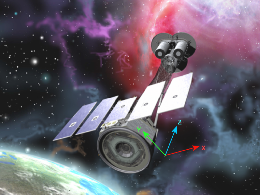
Figure 1: The Imaging X-ray Polarimetry Explorer with the three Detector Units at the focus of the three mirror modules.

A Gas Pixel Detector (GPD), based on the same technology exploited in IXPE (Baldini et al., 2021), was flown on board a CubeSat and is, presently, collecting scientific data from a long observation of the Crab Nebula, with a possible detection of a time variation of polarization of the pulsar (Feng et al., 2020), and other bright sources.

The sensitivity of IXPE is 30 times better than that of the Bragg polarimeter on-board OSO-8, for a 10 mCrab source, while is more then two order of magnitude better then the GPD on board of the Cubesat for a source of the same intensity. While polarimetry of Active Galactic Nuclei was precluded to OSO-8, it is within the reach of IXPE which provides, also, imaging capability in combination with simultaneous spectral and temporal measurements. IXPE’s design is based on the scientific requirements summarized in the Table 1.

A characteristic of IXPE is the dithering during observations. This has been introduced to avoid having to calibrate pixel by pixel, as with Chandra and other observatories with imaging detectors (see Section 6.2). Modern X-ray telescope missions are designed for staring or dithering observation Each detector is mounted, with respect to the next one, on the top-deck of the spacecraft with an angle, around the Z-axis, (the axis of the incoming photon beam, see Figure 1) of 120^∘. Such disposition allow for a sensitive reduction and check of spurious effects.

Table 1: IXPE Scientific Requirements. Half Power Diameter (HPD), Field of View (FOV) and Minimum Detectable Polarization (MDP) are shown

Physical	Observable	Property	Value
Parameter
Linear	Degree $\mathit{\Pi}$, angle $\psi$	Sensitivity MDP99(F${}_{2-8\ }$=10-11 cgs, $\mathrm{\Delta}$t = 10 d)	$\mathrm{\leq}$ 5.5%
Polarization		Systematic error in polarization degree $\mathit{\Pi}$ (5.9 keV)	$\mathrm{\leq}$ 0.3%
		Systematic error in position angle $\psi$ (6.4 keV)	$\mathrm{\leq}$ 1∘
Energy	F(E), $\mathit{\Pi}$(E), $\psi$(E)	Energy band Emin–Emax	2–8 keV
dependence		Energy resolution $\mathrm{\Delta}$E (E = 5.9 keV), $\propto$$\mathrm{\sqrt{}}$E	$\mathrm{\leq}$ 1.5 keV
Spatial	F(k), $\mathit{\Pi}$(k), $\psi$(k)	Angular resolution HPD (system-level)	$\mathrm{\leq}$ 30${}^{{}^{\prime\prime}}$
dependence		Field of view FOV $\mathrm{>}$$\mathrm{>}$ HPD	$\mathrm{\geq}$ $9^{{}^{\prime}}$
Time	F(t), $\mathit{\Pi}$(t), $\psi$(t)	Time accuracy $\mathrm{<}$$\mathrm{<}$ source pulse periods	$\mathrm{\leq}$ 0.25 ms
dependence
Areal	RB/Adet	RB/Adet$\mathrm{<}$$\mathrm{<}$ RS/AS for faint source (2-8 keV, per DU)	$\mathrm{<}$ 0.004 s-1cm-2
background
rate

2 The statistics for an experiment of polarimetry

A detector system can measure polarization if its response is modulated by the polarization of the incoming photons. The photoelectric effect modulates the emission direction of an s-photoelectron as $\cos{{}^{2}}$ of the azimuthal angle, which is the emission angle with respect to the polarization angle. This $\cos^{2}$ dependence is a general feature for a polarimeter. The modulation curve is the angular distribution of the emission directions of photoelectrons in our case and the peak positions determine the polarization angle. The amplitude of the modulation is defined as the semi-amplitude of the modulation curves normalized to its average. If the incoming radiation is 100$\%$ polarized the modulation amplitude is the so called modulation factor $\mu$. This is a key parameter of a polarimeter and spans from 0, if the instrument is not sensitive to polarization, to 1, in case of an ideal polarimeter.

The sensitivity of a polarimeter is expressed in terms of minimum detectable polarization ($MDP_{CL}$) where CL is the confidence level:

$$MDP_{CL}=\sqrt{-2ln(1-CL)}\times\frac{\sqrt{2(C_{S}+C_{B})}}{\mu\times C_{S}}=\sqrt{-2ln(1-CL)}\times\sigma_{P}$$ (1)

C_S are the total source counts whereas C_B are the total background counts. We usually set CL = 0.99 to get the $MDP_{99}$ and we get:

$$MDP_{99}=4.29\times\frac{\sqrt{C_{S}+C_{B}}}{\mu\times C_{S}}$$ (2)

$$MDA_{99}=4.29\times\frac{\sqrt{C_{S}+C_{B}}}{C_{S}}$$ (3)

The minimum detectable amplitude is the minimum modulated signal measurable from a polarized source at 99$\%$ confidence level. It consists of the MDP not normalized by the instrumental modulation factor $\mu$. The raw measurement, indeed, consists of an histogram of photoelectron emission directions (the so-called modulation curve) modulated by the X-ray polarization of the incoming beam.

If a polarization is detected with a modulation amplitude equal to $MDA_{99}$, the measurement is only at about the 3-sigma (Elsner et al., 2012) :

$$n_{\sigma}=\sqrt{-2\times ln(1-CL)}=3.03$$ (4)

Sad to say, but X-ray polarimetry is possible only for relatively bright celestial sources due to the large number of counts needed to build the modulation curve. For a focal plane polarimeters, the background in case of an observation of a point-like source consists, only, of un-rejected events located within the Point Spread Function of the optics. As a matter of fact, for these two reasons the background, for all the point-like celestial sources suitable for polarimetry, is negligible (Xie et al., 2021). The sensitivity, therefore, depends, in this case inversely with respect to $\mu$ and as a square root of the total source counts. In turn the total number of the source counts depends linearly on the observing time $T$, mirror effective area $A_{eff}$, efficiency of the detector $\epsilon$ and source spectrum $S$. In this case the Minimum Detectable Polarization (MDP) can be expressed as:

$$MDP_{99}=\frac{4.29}{\mu\sqrt{SA_{eff}\epsilon T}}$$ (5)

The quality factor of the detector can be expressed as QF = $\mu$ $\times$ $\sqrt{\epsilon}$. A trade-off between $\mu$ and $\epsilon$ provides the best sensitivity to polarization obtainable by the detector.

We also use the Stokes parameters to characterize the polarization. These have the advantage that, as opposed to the degree of polarization and the position angle, they are statistically independent. According to the prescription in (Kislat et al., 2015) we calculated the Stokes parameters of each count. We sum-up the corresponding Stokes parameter to determine the polarization degree and polarization angle of the beam. By fitting a cosine function or summing the Stokes parameter, we obtain the same results.

3 The scientific drivers of the Instrument

IXPE scientific requirements descend from the expected polarization properties of the celestial sources and their temporal, spectral and spatial characteristics. The sensitivity of IXPE, as shown in Table 1, is set for meaningful polarimetry, with realistic observing time, of the brightest AGNs. The residual systematic error in the modulation amplitude should allow for polarimetry below 1$\%$ when observing bright galactic sources. The requirement on the systematics of the polarization angle allows to check possible variation with respect to the old OSO-8 polarimetry of the Crab Nebula. Also, it allows for an effective comparison, at different wavelengths, of phase resolved X-ray polarimetry in combination with the requirement on the timing accuracy. The requirement on angular resolution is derived by the capability to angularly separate the central pulsar from the surrounding torus in the Crab Pulsar Wind Nebula.

Table 2: IXPE Instrument Requirements. Where indicated the 20$\%$ cuts refer to an optimum selection of the data (see for example Section 2) that maximizes the sensitivity considering the events with the most elongated tracks.

Parameter	Requirement
Modulation factor	$>$ 27.7 at 2.6 keV (with 20 $\%$ cut)
Modulation factor	$>$ 53.7 at 6.4 keV (with 20 $\%$ cut)
Spurious modulation	$<$ 0.27 $\%$ at 5.9 keV
GPD quantum efficiency	$>$ 17.7 $\%$ at 2.6 keV
GPD quantum efficiency	$>$ 1.8 $\%$ at 6.4 keV
Energy resolution	1.5 keV (at 5.9 keV)
Knowledge of the spurious modulation	$<$ 0.1 $\%$ at 2-8 keV keV
Systematic error on angle	$<$ 0.4 deg
Position resolution (HPD)	$<$ 190 $\mu$m at 2.3 keV
Dead time	$<$ 1.2 ms (average at 3 keV)
Maximum counting rate	900 c/s
Time accuracy	$\pm$ 94 $\mu$s (99 $\%$)
Background	$<$ 0.004 s-1 cm-2 per DU (2-8 keV)

Table 2 flows down the scientific requirements into instrument requirements. As a matter of fact, polarization sensitivity depends inversely on the modulation factor and inversely to the square-root of the quantum efficiency. The requirement on the modulation factor is more stringent with respect to the quantum efficiency. As a matter of fact a deficit in quantum efficiency results in a linear increase of the observing time to get the same sensitivity. A deficit in the modulation factor requires, instead, a quadratic increment.

The requirement on the maximum allowed modulation amplitude from an unpolarized source was set, initially, only at 5.9 keV because of the availability of a true unpolarized source. A low energy effect (see Section 6.2) was found and characterized.

Time resolution and time accuracy requirement are set accordingly to what the technology offers thanks to the use of a Global Positioning System (GPS) receiver, therefore with a large discovery space in case of pulsating neutron stars either isolated or in binary systems.

The largest contribution to the angular resolution of the telescope system is the HPD of the mirror (Fabiani et al., 2014). The second contribution is the inclined penetration of X-rays onto the detector which has an active volume with 1cm-deep thickness. The third contribution is the position resolution of the detectors which is negligible with respects to the other two. The requirement on the blurring (position resolution) of the detector of Table 2 is set not to spoil the angular resolution of the telescope by more that few $\%$.

The detector has been designed with sufficient FOV when coupled to mirrors having focal length of few meters. With such focal length mirrors are efficient for reflecting X-rays in the classical 1-10 keV energy band. The FOV requirement allows for polarimetry with a single observation of shell-like Supernovae like Cas A, Tycho and Kepler (Soffitta et al., 2013b).

The energy resolution requirement allows for studying energy-dependent phenomena, like, for example, the energy dependent rotation of the polarization angle in galactic black-holes binaries in the thermal state (Stark & Connors, 1977; Connors & Stark, 1977). Moreover this requirement allows for assigning the correct modulation factor, rapidly increasing with energy, to the detected photons deriving the polarization of the X-ray sources.

A small dead-time allows for a minimum decrement of the detected counting rate, and therefore of the sensitivity, from sources as bright as the Crab Nebula. Due to the limitation of the onboard memory and the requirement on the use of the S-band for on-ground data transmission, particular care must be taken to interleave bright source observations with faint source observations.

The background-rate requirement, albeit larger than that of space experiments with gas detectors with front and rear anti-coincidence, allows for measuring polarization from dim and extended sources like molecular clouds in the galactic center region.

4 IXPE payload overview

The IXPE payload (O’Dell et al., 2018, 2019; Soffitta et al., 2020) consists of a set of three identical telescope systems co-aligned to the pointing axis of the spacecraft and with the Star-Trackers. Each system, while operating independently, comprises of a 4-m-focal length Mirror Module Assembly (MMA, Ramsey et al. (2019)) that focuses X-rays onto the respective Detector Units (DUs). Each Detector Unit (DU) hosts one polarization-sensitive imaging detector, with its own electronics, which communicates with a Detector Service Unit (DSU) interfaced to the spacecraft Integrated Avionics Unit (IAU). The three DUs and the DSU are collectively called the IXPE Instrument. The DUs are mechanically mounted onto the top deck of the spacecraft oriented, as already mentioned above, with a rotation of 120^∘ each with respect to the beam axis (Z-axis see Figure 1).

The performance of the detectors and, particularly, the gain, have to be monitored during the operative life of the mission. Other parameters like the modulation factor, are expected, from ground calibration, to be more stable in time but they can be monitored as well. For these reasons each DU is equipped with a multi-function filter and calibration wheel assembly that allows for (i) in-flight calibration of the modulation factor,(ii) the calibration of the gain, (iii) source flux attenuation (iv) background measurements. MMA and DUs are separated by an able to be deployed (3.5 m) boom; the position of the MMA with respect to the DUs can be adjusted after deployment with a Tip/Tilt/Rotate mechanism. Each MMA hosts an X-ray shield to avoid, in combination with a stray-light collimator mounted onto the top of the DU, X-ray photons impinging on the detector active area when arriving from outside the telescope field of view. The use of a set of telescopes provides many advantages with respect to a configuration based on a single telescope of equivalent collecting area. First of all, since the energy band-pass fixes the ratio between the mirror diameter and the focal length, a multiple telescope configuration is more compact than a single larger telescope; this occurs at the cost of an increase of the measured background which, however, is not a driving requirement for IXPE. Moreover, a multiple system is intrinsically redundant and offers the possibility of comparing independent data and to correct small effects which may mimic a real signal.

5 The design of the instrument

The design of the instrument, and in particular the design of the DUs, is the consequence of the prescription of using the Pegasus XL launcher at the time of the proposal. The top-deck of the spacecraft hosts at launch both the three un-deployed mirrors and the three DUs. Hence, the available space in the top deck requires a vertically stacked mechanical configuration for the DUs. Such configuration is demanding in terms of thermal dissipation and, in addition, has a worse response to vibrations than a side-by-side configuration. In the following phase of competitive bidding during phase B, a Falcon-9 was eventually selected and will lift IXPE to the foreseen 600 km equatorial orbit.

The IXPE Instrument, mainly supported by the Italian Space Agency, ASI, has been entirely designed, built and tested in Italy. We show the items of the Instrument as Italian IXPE contribution in Figure 2. In the same figure the responsibilities for each item that are shared between INAF, INFN and the industrial partner OHB-Italy are shown.

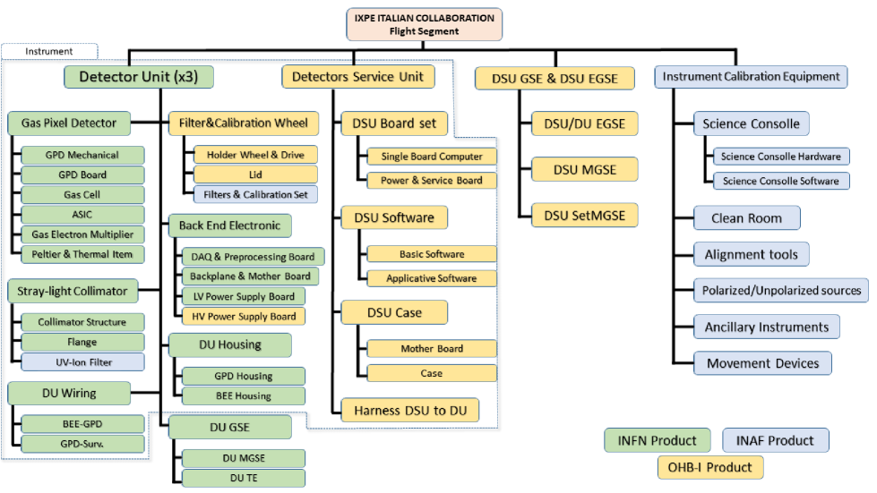
Figure 2: Instrument Product Tree.

Each of the four DUs (including one spare unit, see Figure 3), comprises the following sub-units:

1. Gas Pixel Detector (GPD), which is an X-ray detector with gas as the absorption medium and a Application-Specific Integrated Circuit (ASIC) as the readout electrode, specifically developed by INFN in collaboration with INAF-IAPS for X-ray polarimetry.

2. Filter & Calibration Wheel (FCW), which hosts the calibration set comprising calibration sources and filters for specific observations to be placed in front of the GPD when needed.

3. Back End Electronics (BEE), which comprises of electronics boards (DAQ, Data Acquisition Board, Barbanera et al. (2021) to manage the GPD ASIC), the required High Voltage lines and the Low Voltages lines.

4. Stray-light Collimator (STC), already mentioned above.

5. DU Housing (DUH), which provides the mechanical and thermal interface of the DU to the S/C.

6. DU wiring (DUW), which provides the electrical interfaces (internal to the DU) between the BEE and the GPD.

The DSU is the unit which provides the DU with the needed secondary power lines, controls and powers the FCW, formats and forwards the scientific data of the three DUs to the spacecraft. The DSU comprises the following sub-units:

1. DSU Board Set (DBS), which is the set of electronic boards (both nominal and redundant) which perform the DSU tasks;

2. DSU Software, which comprises the software which runs in the DSU;

3. DSU Case (DSC), which includes a back-plane that provides the electrical interface among the DSU boards. Further, the DSU Case provides the mechanical and thermal interface of the unit;

4. Harness DSU to DU, which comprises the cables necessary to electrically interface the three DUs to the DSU.

Moreover, to complete the instrument related units, two testing/calibration stations were assembled. One is the Instrument Calibration Equipment, which is shortly described in Section 9, and the companion Assembly Verification and Test Equipment. The latter has three positions, one for each DU. Each testing/calibration stations consist of X-ray sources, collimators, crystals and computer controlled stages to calibrate the DUs and to perform the bench integration of the instrument. The Electrical Ground Support Equipment has also been assembled to manage the DUs and DSU calibration activities and bench integration.

In this paper we present the status of the instrument before the assembly with the spacecraft. However, due to its design, any change of performances after the integration is not expected.

6 The IXPE Detector Unit

In order to save space, the DUs were designed with a top-bottom configuration for the detector and associated electronics respectively. The 120^∘ clocking allows for checking the level of absence of spurious modulation and limiting any systematic effects. The exploded view of the DU and a picture of one assembled DU is shown in Figure 3.

The DU housing is composed of two boxes. The top one is the ”GPD housing”. The bottom item is the ”Back-End Housing”. In the next sections we describe the main elements of the DUs.

6.1 Stray-light collimator and UV-ion filter

An extensible boom connects the mirror modules to the spacecraft top-deck. This open-sky configuration requires a system to prevent that Cosmic X-ray Background photons arriving from outside the mirror field of view impinge on the detector. At this aim, a tapered stray-light carbon-fiber (CF) collimator collects only the photons reflected by the optics, thanks, also, to fixed X-ray shields around the mirror modules. The thickness of the collimator is 1.25 mm and includes the 1-mm thick CF with an external 50-$\mu$m molybdenum coating and 20 $\mu$m gold of the molybdenum foil.

Due to the fact that the beryllium window of the detector and the supporting titanium frame is at high potential (about -2800 V) positive ions may interact with the top GPD structure producing eventual secondary photons and a possible failure of the high voltage system. For this reason, photons from the optics cross a UV-ion filter made by LUXEL composed of 1059 nm of LuxFilm^® (based on kapton) with an external coating of 50 nm of aluminum and an internal coating of 5 nm of Carbon. The UV-ions filters are described in La Monaca et al. (2021). The scope of UV-ions filter is to prevent UVs and low velocity plasma present in orbit for reaching the beryllium window of the GPD (see Section 6.2). The transparencies at two energies are reported in Table 5.

Figure 3: The IXPE Detector Units (a) Exploded view of a Detector Unit, (b) Photograph of a Flight Detector Unit in its handling plane. The thermal environment is controlled by means of a Peltier cooler and a heater. A thermal strap conducts the heat from the GPD Peltier/heater system to the radiator of the spacecraft.

6.2 The Gas Pixel Detector in the Detector Unit

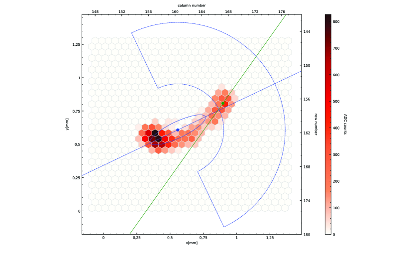
Figure 5: Real photoelectron track at 5.9 keV with reconstructed direction of emission and absorption point.

The GPD (see Figure 4), located in the GPD housing, is a gas detector for which the charge-signal is readout by a matrix of 105k pixels (300 $\times$352 pixels arranged in a 50 $\mu$m pitch hexagonal pattern) of a dedicated, custom Complementary Metal-Oxide Semiconductor (CMOS) ASIC (Bellazzini et al., 2006). The custom ASIC has self-triggering capabilities thanks to local triggers defining each group of four pixels called mini-clusters. Each event consists of a Region of Interest (ROI) made by all the mini-clusters that trigger plus a selectable additional fiducial region of 10/20 pixels. The charge content of each pixel in the ROI is readout serially from a single buffer as differential current output by means of a 5 MHz clock. The ASIC, also, provides the absolute position of the ROI as digital coordinates of two opposite vertices and the global trigger output, about 1$\mu$s after the arrival of the charge. The threshold is set low enough to collect signals coming from events which release about 300 eV. The charge amplification is provided by a Gas Electron Multiplier (GEM), a thin 50 $\mu$m dielectric (liquid crystal polymer) foil with 9-$\mu$m copper metallization on both sides. Through-holes are laser etched and disposed on a regular triangular pattern with vertexes 50$\mu$m apart. These cylindrical holes have a diameter of 30 $\mu$m (Tamagawa et al., 2009; Tamagawa & et al., 2010). The basic building blocks of the GPD assembly and their functions are schematically illustrated in Figure 4. The small pitch of the ASIC and the GEM are responsible for the good image of the photoelectron track (see Figure 5).

In summary, the GPD is composed of the following subassemblies:

1. mechanical interface (GPD Mech. I/F), made of titanium, which supports the GPD unit, connects it to the focal plane and provides references for alignment with the MMA;

2. printed circuit board (GPD Board), which connects the GPD to the readout electronics;

3. ceramic spacer (GEM Support Frame), supporting and insulating the GEM from the GPD Board; the lower gas gap of 770 $\mu$m for the drift of the amplified electrons is defined by the ASIC top surface and the bottom GEM.

4. the GEM foil (GEM), including four soldering pads for the high voltage connections;

5. ceramic support (Drift Spacer), which defines the absorption gas cell above the GEM and isolates the GEM from the top electrode;

6. titanium frame (Ti frame and Be window) which closes the gas cell and allows X-rays into the GPD through the integrated thin, optical-grade 50 $\mu$m one-side aluminized beryllium window. The titanium frame and the beryllium window serve, also, as a drift electrode;

7. filling tube of Oxygen Free High Conductivity copper and its fixture to the titanium frame (tube and fixture);

The GPD is sealed and does not require any gas cycling systems. The keystone of the assembly is the Kyocera package. In fact the ASIC is designed to fit into a commercial package that acts as the bottom parts of the gas cell and connects the internal wiring and the clean gas volume to the external Printed Circuit Board (PCB), onto which the package is soldered. In this way cleanness is preserved in the gas volume.

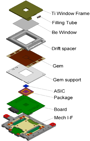
Figure 4: Schematic representation of GPD assembly.

The GPD assembly is done at INFN, whereas the filling procedure is performed at Oxford Instruments Technologies Oy (OIT, Espoo, Finland). After a vacuum leak-tightness check, the GPD is continuously baked-out and pumped-down for 14 days at 100 ^∘C for outgassing and eliminating possible impurities in the internal gas cell. Finally the GPD is filled with a Dimethyl-Ether (DME) mixture at 800 mbar at room temperature. OIT filled with the same gas mixture a single-wire proportional connected in parallel to the same filling station to check the energy resolution. If the energy resolution is within the requirement, the filling tube of the GPD is crimped. We selected this three-times distilled gas mixture because it minimizes track blurring thanks to its small transverse diffusion ($\frac{69\mu\textrm{m}}{\sqrt{\textrm{cm}}}$ at 1833 V/cm and 0.8 bar). Its pressure is optimized in order to provide the best combination of efficiency and modulation factor and, therefore, the sensitivity in the energy range of interest. Indeed a lower pressure increases the track length, but also the diffusion and reduces the quantum efficiency. A larger pressure, instead, increases the quantum efficiency but reduces the track length and this reduction is not compensated in terms of modulation factor by the simultaneous reduction of diffusion. In Section 7.1 we will describe a peculiar phenomenon called ’virtual leak’ that reduces asymptotically the pressure at 640-650 millibar increasing the track length.

Three negative high voltages are required by the GPD. The GEM bottom voltage (V_bottom on the side facing the ASIC) sets the electric field in the transfer gap between the GEM and the ASIC. The difference between the GEM top voltages (V_top on the side facing the window) and V_bottom sets the gas gain. The high voltage on the titanium frame and beryllium window, (V_drift) sets the drift voltage in the absorption region in combination with the V_top.

The performance of the GPD is, in principle, dependent on temperature to some extent. The GPD temperature is controlled during the operation by means of a Peltier cooler and heaters. A thermal strap connects the cooler directly to the spacecraft radiator. The GPD thermal control is performed directly by the DSU and is designed to be as independent as possible from the BEE temperature, since the latter has much looser requirements. The Peltier cooler and the heaters, and the thermal dissipation of the spacecraft, maintain the temperature of the GPD within the range 15-30 ^∘C.

7 The physical quantities provided by the GPD

Thanks to the GPD, all the information contained in the observed X-ray radiation is provided to the user, after that a proper algorithm is applied to the data (see Section 11). The projection of the track onto the hexagonally patterned top layer of the ASIC is analyzed to reconstruct the point of impact and the original direction of the photoelectron. The impact point, not the charge barycenter, gives an imaging resolution which is better than 190 $\mu$m in diameter (Soffitta et al., 2012). The eventual spatial resolution of the instrument is due to the diffusion of the initial track, to the reconstruction algorithm capabilities and to the quantization of the GPD pixel size.

The energy is estimated by summing the charge content of each pixel.

The event time is determined by the trigger output of the ASIC. Compared with a Charge-Coupled Device (CCD) currently flying in most of the space mission with X-rays optics, no pile-up issue is present because of the fast drift time (1 cm/$\mu$s) coupled with the fast inhibition to additional charge processed by the ASIC.

The linear polarization is determined by the angular distribution of the emission directions of the photoelectron tracks in the selected energy band. This is called the modulation curve. If the radiation is polarized, the modulation curve shows a cosine square modulation, whose amplitude is proportional to the degree of polarization and whose phase coincides with the angle of polarization. The amplitude of the modulation of the incident beam is eventually normalized to the modulation obtained for 100 $\%$ completely polarized photons (the so called modulation factor $\muup$) to get the beam polarization. The energy dependant modulation factor of the GPD is measured at different discrete energies during the calibration campaign of the detector and well agrees with predictions derived by accurate Monte Carlo simulations.

During the construction phase of the instrument, and in particular of the Gas Pixel Detector, we detected a non-zero modulation from unpolarized radiation. This signal is called spurious modulation. The amplitude of this signal is of the order of 1.5 $\%$, on each DU, at 2 keV rapidly declining with energy. The root cause of this spurious modulation is not totally understood yet, but we have identified a few effects that contribute to it by systematically deforming the photoelectron track. Some of them, collectively called “ASIC effects”, originate from small systematic biases in the ROI reading. These are typically tiny, i.e., a fraction of the pixel electronic noise in amplitude, yet they cause a measurable effect on large number of counts. They were minimized by an appropriate choice of the read-out clock frequency and eventually canceled out by subtracting the residual measured bias from the data in the off-line analysis. Another contribution to spurious modulation comes possibly from the deformation of the track during multiplication, as is suggested by the correlation between the gain spatial mapping and the spurious modulation spatial mapping. In order to subtract the spurious modulation from the data we organized a vigourous calibration campaign for each DU in such a way to dedicate most of the time to characterize this effect. We used several nearly unpolarized sources at different energies and on different regions of the detector, from 2 keV up to 5.9 keV where this effect vanishes. More details on the calibration campaign are reported in 9.

7.1 Short $\&$ secular gain variation

A short-term rate-dependent gain decreasing, accompanied by a secular gain increasing, was also detected. The first one is due to charging effects on the exposed dielectric by drifting ions and electrons during the multiplication process. The second is likely due to an absorption or adsorption of the gas by materials inside the GPD. These two effects have been studied in detail. The first effect is described by simple functions applied by the processing pipeline to the data for gain normalization. The second effect is expected to saturate at an average 640-650 mbar already by the time of the flight as indicated by the gain, the counting rate from a ${}^{55}Fe$ reference source and the track length trends. All these parameters are, simultaneously, well modelled in ten detectors including the three flight DUs, the spare DU and the GPD control sample (Baldini et al., 2021). The impact is a decrement of the quantum efficiency, however the accompanying increase of the modulation factor reduces the loss of sensitivity to an acceptable level.

7.2 The Filters and Calibration Wheel

The filter and the calibration wheel (FCW) has been designed to monitor the performance of the detector during the life of the mission. In particular we intend to check the low and high energy modulation factor and the spurious modulation during the observational life of the mission. Also we monitor the gain that depends both on temperature and on charging (see Section 6.2 and 7.1).

The FCW hosts filters to perform special observations (e.g., very bright sources) and calibration sources to monitor detector performance during flight. The FCW has 7 positions commanded by the DSU. The positions correspond to open position, closed position, gray filter and calibration source A, B, C and D. The stepper motor is a Phytron phySPACE^TM 42-2. It is a COTS component with 25 years of space flight heritage. The phySPACE^TM series is developed and built to resist vacuum, vibrations, low/high temperature and radiation while maintaining high performance, precise positioning and long life. The motor pinion is made of Vespel^®. The double bearing system that connects the fixed part to the rotating one is made of stainless steel. The positioning is performed and monitored by two different systems.

One system is based on the use of Hall sensors as non-contact switches to stop the wheel rotation at the requested position. A combination of three hall sensors allows for setting and monitoring the 7 wheel positions.

In order to have an independent measurement of the wheel position a second, analog, device, a Novotechnik PRS65/S152 potentiometer, is implemented. A qualification campaign allowed for declaring this component as flight compatible.

The FCW positioning can be set digitally or on’ a step-by-step basis permitting gain and modulation factor to be measured at various positions on the detector.

The calibration set is composed of the X-ray sources and their holders. It comprises the items which can be put in front of the GPD by rotating the FCW. The design of the calibration set is shown in Figure 6.

Figure 6: CAD models of the calibration set. All sources are derived from capsules containing an ${}^{55}Fe$ nuclide: (a) Cal A is the polarized source. It is un-collimated and provides simultaneous polarized X-rays at 3.0 keV and 5.9 keV, (b) Cal B is an unpolarized collimated 5.9 keV source, (c) Cal C is a broad 5.9 keV source for flat field illumination, (d) Cal D is a broad 1.7 keV source for gain and spurious modulation check-out

In the following we summarize the particular positions which are also described in Ferrazzoli et al. (2020):

1. Open position. The open position is the standard one used for astrophysical observations.

2. Closed position. The closed position has two motivations. It is a safe position for the instrument, but it is also necessary to gather instrumental (internal) background to be compared with that obtainable during Earth occultation.

3. Gray filter. Because of the relative large, ($>$ 1 msec) dead-time, of the Gas Pixel Detector and the available throughput from the bus and from the down-link, we decided to include a partially opaque absorber. This partially opaque absorber is designed to be used when the count-rate is greater than that produced by a source about 4 times more intense than the Crab or greater. It absorbs efficiently low-energy photons where the count-rates are greater. At higher energies, where the count-rates are smaller the absorption is small. The filter is made of 75-$\mu$m thick kapton foil with 100 nm aluminum on both sides. For a Crab-like spectrum (power law with index 2) the flux will be reduced of a factor about 6 in the 1-12 keV energy band. The measured energy dependent transparency is shown in Figure 7.

4. Calibration source A (Cal A). This source produces polarized X-ray photons at two energies (3.0 keV and 5.9 keV) to monitor the modulation factor of the instrument in the IXPE energy band. An exploded view of this source is shown in Figure 6. A single ⁵⁵Fe nuclide is mounted and glued into a T-shaped holder. X-rays from ⁵⁵Fe at 5.9 keV and 6.5 keV are partially absorbed by a thin silver foil mounted in front of the ⁵⁵Fe nuclide to produce fluorescence at 3.0 keV and 3.15 keV. The silver foil is 1.6 $\muup$m thick and is deposited between two polyimide foils which are 8 $\muup$m (on the side towards the ⁵⁵Fe) and 2 $\muup$m (on the opposite side). Photons at 3.0 keV and 5.9 keV, broadly collimated, are diffracted by a graphite mosaic crystal, with FWHM mosaicity of 1.2 deg, at first and second order of diffraction, approximately at the same diffraction angle (about 0.5^∘). A diaphragm is used to block the stray-light X-rays except the scattered X-rays from the graphite.

5. Calibration source B (Cal B). This source produces a collimated beam of unpolarized photons to monitor the degree of spurious modulation. An ⁵⁵Fe radioactive source is glued in a holder and screwed in a cylindrical body. A diaphragm with an aperture of 1 mm collimates X-rays from the ⁵⁵Fe to produce a spot of about 3 mm on the GPD; such a spot has a size which is representative of the source image of a point-like source when the spacecraft dithering is included.

6. Calibration source C (Cal C). This source will illuminate all the detector sensitive area to map the gain at one energy. This source is composed of an ⁵⁵Fe iron radioactive source glued in a holder which is screwed in a body. A collimator allows X-ray photons to impinge on the detector sensitive area only when the source is in front of the GPD.

7. Calibration source D (Cal D). This source will illuminate all the detector sensitive area as does the Cal C, to map the gain at another energy. Cal D is based on an ⁵⁵Fe source, glued in an aluminum holder which illuminates a Si target mounted on a body to extract K$\alphaup$ fluorescence from silicon. This source produces fluorescence emission at 1.7 keV. Silicon would provide, together with Cal C, more leverage for gain calibration and, since photoelectron tracks are smaller at this energy, the gain map can have a higher spatial resolution. It is worth noting that the design is such that X-ray photons from ⁵⁵Fe cannot directly impinge on the GPD sensitive area to avoid detector saturation.

All calibration sources inside the FCW contain an ⁵⁵Fe nuclide, whose activity naturally decays with a half life of 2.7 years. In Table 3 we report the expected flight rate at the beginning of the operative phase of IXPE that, at the time of writing, is on November 2021.

Table 3: The nominal activity at the beginning of life and the averaged counting-rate expected at the beginning of the IXPE operative life, assumed to be on November 2021

Calibration Source	Activity (mCi)	Counting rate (c/s)
Cal A	100	1.4 @ 3.0 keV
		17 @ 5.9 keV
Cal B	20	48 @ 5.9 keV
Cal C	0.5	90 @ 5.9 keV
Cal D	100	76 @ 1.7 keV

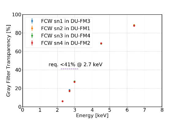
Figure 7: The measured transparency of the gray filter used in each DU.

Replacement/installation of the radioactive nuclide is possible through a dedicated opening in the DU lid. Radioactive sources, glued in their holders, can be extracted with dedicated tools and replaced with new ones in new holders.

8 Detector Service Unit

Thanks to the functionalities of the ASIC and of the GPD readout system, most of the necessary operations on the data are performed by the DAQ electronics (Barbanera et al., 2021) including acquisition, digitation of the pixel charge, zero-suppression and efficient data packing. We designed the DSU in order to, mainly, perform data formatting in a way suitable for the storing into the spacecraft memory (5 GByte) and for using the S-band for downloading. The DSU also controls the Filter $\&$ Calibration Wheels and manages the payload operative modes.

The DSU provides the following functions for the operation and autonomy of the IXPE instrument:

1. Power supply generation (secondary power to supply the DU’s sub-units)

2. Telemetry management (data acquisition, formatting and transmission to the S/C)

3. Commands management (reception, verification, generation, scheduling, distribution or execution)

4. Time management (synchronization of the DUs, Pulse Per Second (PPS) distribution and time tagging)

5. Filter and Calibration wheel management

6. Science data management (retrieving, isolated pixels removal, formatting and transmission to the S/C)

7. Payload mode control

8. GPD temperature control

9. Fault Detection Isolation and Recovery (FDIR) management

The DSU consists of two boards, with cold redundancy, and one backplane for internal DSU signal routing. The boards are the Single Board Computer (SBC) and the Power & Service Board (PSB).

Figure 8 shows the high level architecture of the DSU with its main electrical interfaces.

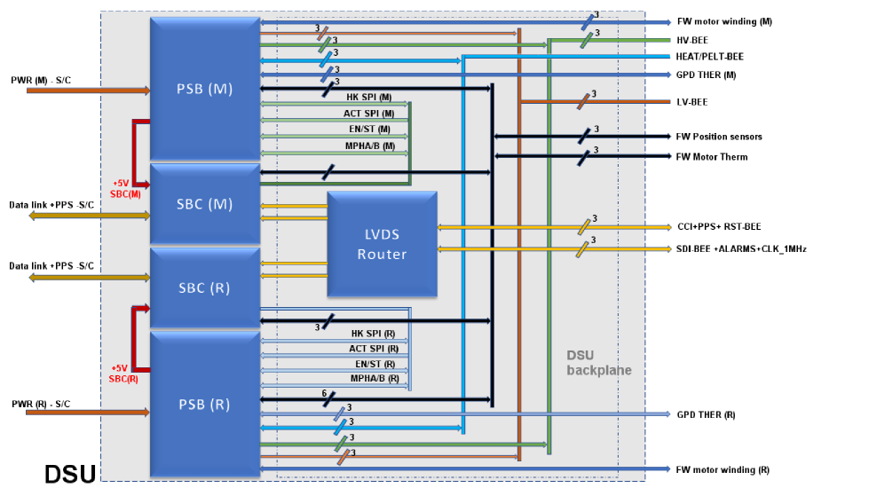
Figure 8: DSU high level architecture.

The SBC implements the instrument control and configuration and the instrument data processing and formatting. In fact, it performs a rejection of raw data called ’orphan removal’ (see Section 8.2). The SBC is based on a LEON3FT Central Processing Unit (CPU). The LEON3FT CPU is implemented in ASIC provided by COBHAM (UT699). A companion Field-Programmable Gate Array (FPGA), belonging to RTAX family by MICROSEMI, is included to support the processor operation and to provide the management of data interfaces required by the IXPE instrument and not included in the ASIC.

The PSB performs different tasks relevant to power management; in particular, this board hosts the power converters aimed at the generation of required supply voltages both for DU and DSU electronics. The drivers for DU thermal actuators (heaters and Peltier cells) and for the FCW are also installed. The DSU, also, implements the signal conditioning for the Resistance Temperature Detectors (RTD) of the DU temperature control and for the motor positioning sensors of the FCWs and their temperature.

DSU architecture supports a redundancy philosophy based on cold-sparing approach. The only exception is the power I/F for each FCW motor that is equipped with redundant coil for each motor phase. For each motor phase, the main coil is connected to the main PSB motor driver and the redundant coil to the redundant PSB motor driver. For this reason, one temperature sensor is connected to the main PSB and the other one to the redundant PSB.

The data interface between DSU and each DU consists of the following 5 sets of three signal lines which comply with Low-Voltage Differential Signal LVDS standard:

1. Three Command and Communication Interfaces (CCI) for command transmission from DSU to each DU

2. Three Serial Data Interfaces (SDI) for sensor data transmission from each DU to DSU

3. Three reset lines, one for each DU

4. Three input alarm lines, one for each DU, used to switch off the relevant DU in case of anomaly detected by the BEE

5. Three output timing signals for DU internal acquisition timing verification

IXPE uses a centralized spacecraft memory bank for data storage and transmission. The memories on-board the DSU are used only to store the boot SW and support the CPU and FPGA operation.

The local bus connects the LEON3FT CPU, the FPGA, the central SRAM (Static Random Access Memory), the PROM (Programmable Read Only Memory) and MRAM (Magnetoresistive random-access memory). In order to minimize bus loading, the MRAM is connected to the local bus via bus switches. After boot phase completion, the MRAM is disconnected from the bus.

The DSU interfaces the Spacecraft with two (one Nominal and one Redundant) unregulated power lines on separate connectors. The nominal voltage of the power lines is 28 V. Minimum and maximum values of input power provided by S/C is respectively 26 V and 34 V.

8.1 IXPE instrument timing architecture

The IXPE satellite manages the timing of the events using a GPS receiver. The GPS provides a PPS received by the instrument through a dedicated line. The Spacecraft also provides the Time of the Day (TOD) with a frequency of 1 Hz. The TOD contains information about the validity of the previously provided PPS and the time of the next PPS. A plot showing the timing scheme is shown in Figure 9.

The DSU is equipped with a temperature compensated crystal oscillator (TCXO) with an accuracy $\mathrm{<}$ 4ppm. The PPS and the 1 MHz clock generated by the 1 MHz local oscillator are provided to each DUs.

The On-Board Time (OBT) management is based on a Master OBT implemented in the DSU and 3 Local OBTs implemented in the DUs. The Master OBT and the Locals OBTs are composed of (i) a 29-bit counter for the seconds ($\mathrm{>}$ 16 years of mission lifetime) and (ii) a 20-bit counter for the microseconds (1 $\mu$s resolution) and a register for the OBT error (error counter).

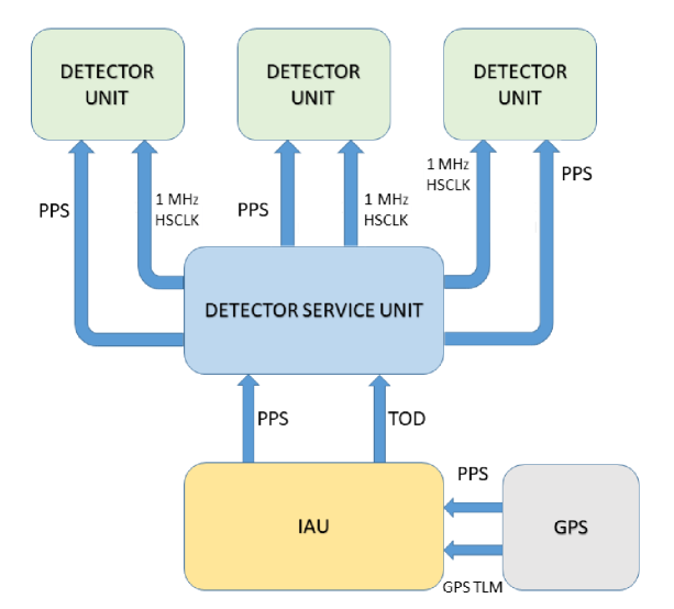
Figure 9: The Architecture of timing for the instrument.

At boot, the Master OBT is initialized by subtracting the Start Mission date (stored in the DSU MRAM) from the GPS time.

During nominal observation, when the GPS is valid, the second counter is incremented upon receiving the PPS and the microsecond counter is incremented by the 1 MHz local oscillator. At the arrival of the PPS, the difference of the microsecond counter with respect to 10⁶ is stored in the Master OBT error counter and included in the Housekeeping packet data with 1 $\mu$s resolution and 1 s rate. The Local OBTs are updated in the same way by the FPGA located in the BEE using the PPS provided by the S/C through the DSU and the 1MHz clock provided by the DSU.

If the previous PPS is not valid, as indicated by the TOD, the PPS provided by the S/C is not used. The DSU synthesizes the PPS for the DUs using the Local TCXO. During this operation mode the OBT Error is set equal to zero. The non-valid condition information is included in the Housekeeping (HK) data. The Master OBT remains in free running until the reception of the sequence of TOD reporting that the PPS is newly valid. In this case the DSU re-initializes the Instrument timing as at Instrument boot.

The alignment of the Local OBT with the Master OBT is verified using the housekeeping telemetry (TM). The HKs Telemetry (TM) comprises the values of the Locals OBT and the Master OBT every second. At the MOC/SOC these values are monitored and in case of misalignment an action recovery is planned (e.g., Time Reset by telecommand).

8.2 Orphan removal of data

The fulfillment of the requirement on the maximum counting rate is possible thanks to the DAQ that packs consecutive zeroes by writing their number in a single word (Barbanera et al., 2021) and the isolated pixel removal in the DSU. As a matter of fact the only data processing made on-board by the DSU is the removal of isolated pixels (called orphans in the photoelectron track image) generated by noise. This removal is performed with a simple algorithm on the serial stream of the zero-suppressed data delivered by the DU for each event. It requires a limited memory allocation and is performed by the FPGA without impact on the CPU timing. By means of the packing in the DU and the removal of isolated pixel it is possible to reduce the data rate within the requirements for the S-band. In fact, only the pixels that identify the tracks are down-loaded, suppressing the isolated pixel generated by noise.

8.3 Instrument Operative Mode Specifications $\&$ Transitions

The Instrument operative modes are managed by the DSU and they are selected either via telecommand, or by activating autonomously a FDIR procedure. The BEE is controlled by the DSU, and only if it generates an alarm condition, the DSU responds setting the instrument in Safe mode. The transition between modes is described by Figure 10.

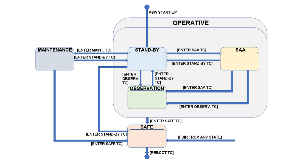
Figure 10: The operative modes of IXPE payload and the transition via telecommand and FDIR.

The foreseen payload operative modes are the following:

• Boot (transitional mode). BOOT is the start-up mode at power on. A limited SW application, called Boot Software, runs from the Programmable Read Only Memory (PROM) in order to perform all the checks and the initialization of instrument resources and items. In the nominal case the Application Software (ASW) completes the initialization sequence execution by entering the instrument in STAND-BY. The boot phase lasts around 60 seconds.

• Maintenance. This mode is reserved to support the in-orbit maintenance program. This mode can be reached on request when the DSU SW mode is in Stand-By and is dedicated to memory management operations like code and data load/download in/from MRAM and SRAM.

• Stand-by. Nominally, at the end of the boot-strap phase, the DSU moves in Stand-by mode to start the instrument monitoring and control. The stand-by mode supports the starting and handling of the thermal regulation, powering on and off the instrument items, the processing of the incoming telecommands and the generation of the related TM. Finally it configures the detector units and the science data processing.

• Observation. From the point of view of the DSU, all instrument calibration and scientific modes are managed into a unique Observation mode that is preventively configured while in Stand-by mode. This mode supports the handling of thermal regulation, the handling of the Time of Day message, the collection of the housekeeping and the generation of scientific data.

• South Atlantic Anomaly (SAA). This mode is used when the satellite crosses the South Atlantic Anomaly that happens once per orbit. In this mode, the High Voltage (HV) are ramped-down below the voltage that sets multiplication, the science data generation is disabled while housekeeping data are generated and collected as usual.

• Safe. This mode is used before switching-off the instrument or performing a SW reboot and managing the FDIR conditions. This mode preserves DUs and HVs status (i.e., no ramp-off or switch off are performed on hardware) when entered by telecommand. If entered by FDIR, HVs ramp-off, DUs switch off and FCW rotation to CLOSE can be performed as part of the Recovery action. In this operative mode, the instrument generates and collects the housekeepings. Only during Safe mode it is possible to perform a reboot of the ASW.

• Reboot (transitional mode). At the DSU switch-on, after the BOOT SW activities the ASW is loaded into SRAM and executed. The ASW checks the position of the Filters and Calibration Wheels and the status of the Detector Units and High-Voltages Boards.

  If the FCWs are closed and the HVBs are off, the ASW moves to STAND-BY mode. If the FCWs are not closed or if the HVBs are ON, the ASW moves the FCWs to CLOSED position, performs the ramp-off procedure if HVBs voltages are greater than zero, it switches off the DUs, it moves SW operative mode to Safe.

9 The Calibration of the IXPE Detector Units

Being a discovery mission, celestial sources are not available for performing in-flight calibration for polarimetry. In fact the measurement performed 45 years ago on the Crab nebula (Weisskopf et al., 1978b) with a non-imaging detector, cannot be used as a ’flight’ calibrator. Indeed this time interval is already about 5 $\%$ of its lifetime and the Crab-nebula was found to vary. For these reasons an on-ground detailed calibration is mandatory.

Furthermore we designed and built an on-board calibration system aimed at checking variations in the modulation factor and, even if not with the same accuracy reached on-ground, any variation on spurious modulation (see Section 7.2)

The calibration of the Detector Units is a key activity for IXPE, Details of the calibration facility and of the calibration results will be presented in forthcoming papers. Beside validating the Monte Carlo prediction for the modulation factor, more importantly it provides physical parameters like (i) the low-energy spurious modulation which is the instrument response to unpolarized radiation (see Section 6.2 and Figure 12) and (ii) the gain non-uniformities that cannot be modelled in advance: they have been calibrated on ground and included in the data processing pipeline. The calibration strategy mimics the observation strategy during flight that foresees dithering of point-sources. In this way, when we calibrated the entire detector, we obtained the so called Flat Field (FF) measurements. When we calibrated at high count rate density only a selected central part of the detector active region, we obtained the so called Deep Flat Field (DFF) measurements. The latter are aimed at reaching very large statistics within the dithering region foreseen in flight for point-like celestial sources. When we calibrated with a narrow beam (less than 1-mm diameter), we obtained the so called ’spot measurements’.

The calibration activity (40 days for each DU) was directed toward measuring the following physical quantities:

1. Spurious modulation (60$\%$ of the calibration time) at 6 energies between 2 keV and 5.9 keV in a DFF configuration (central region with 3.25 mm diameter at a density of 10⁶ counts/mm²) and FF configuration (all detector sensitive area with 10⁵c/mm²)

2. Modulation factor (17.5$\%$ of the calibration time at 7 energies), and different polarization angles, between 2.0 keV and 6.4 keV in DFF configuration (3.25 mm radius, 10⁴ counts/mm²) and in FF configuration (7 mm radius with the same statistics of DFF but in a larger area)

3. Efficiency at, at least, three energies (2.5$\%$ of the calibration time)

4. Spatial resolution (2.5$\%$ of the calibration time) of unpolarized radiation at 3 energies in an array of 3 $\times$ 3 spots

5. Spatial resolution (2.5$\%$ of the calibration time) of polarized radiation at 3 energies in one point

6. Grey filter transparency at 5 energies, inclined penetration (focusing effect) and calibration of the FCW sources (rest of the fractional time)

From the above measurements it was possible to derive, also, the following physical quantities:

• Accuracy of the polarization angle measurement at 7 energies

• Map of the gain variations in the active region

• Measurement of the energy resolution at different energies

• Measurement of the dead time at different energies

We measured the modulation factor at different angles not only to measure the accuracy of the polarization angle but also to check that spurious modulation is properly subtracted. Indeed any change of the modulation factor with polarization position angle is expected in the presence of spurious effects which mimic the presence of a secondary, albeit small, polarization component.

We organized the calibration in such a way that the time dedicated to measure spurious modulation at different energies accounts for 60$\%$ of the total calibration time. As a matter of fact, in order to measure spurious modulation at a level of 0.1$\%$ across the sensitive area, we collected tens of millions of counts for each energy. The calibration time was set considering the maximum counting rate allowed for the DUs, due to their dead time, and the power of the X-ray tubes.

In order to perform such calibrations we built two stations. One station is the main calibration station (called ICE, Instrument Calibration Equipment). The other, called AIV/T Calibration Equipment (ACE) is designed to illuminate contemporaneously up to three DUs to support the integration and test of the whole instrument, but it can host the same calibration sources as the main station. During some periods, ACE was indeed used to carry out calibration measurements in parallel with ICE. They are the so called AIV$\&$T Calibration equipment (ACE1 and ACE2).

The ICE is derived from an earlier design which was used for 15 years at INAF-IAPS (Muleri et al., 2008b, 2021). In particular, it includes:

1. the X-ray sources used for calibration and functional tests. Each source emits X-ray photons at known energy and with known polarization degree and angle. Polarized sources exploit Bragg diffraction at nearly 45^∘ from a set of crystals (see Table 4) with suitable X-ray tubes. Unpolarized sources are based on the direct emission from X-ray tubes or on the extraction of fluorescence emission from a target. The direction of the beam, the position angle for polarized sources, and its position can be measured with respect to the GPD thanks to its fiducial points and the use of a Romer measurement Arm.

2. the test detectors, one commercial Silicon Drift Detector (SDD) by AMPTEK and one X-ray CCD camera by Andor. They are used to characterize the beam before DU calibration and as a reference for specific measurements (e.g., the measurement of quantum efficiency with the SDD).

3. all the electrical and mechanical equipment required to support the DU and the calibration sources, monitor the relevant diagnostic parameters and assure safety during calibrations.

The ICE in the configuration with the polarized source is shown in Figure 11. The DU is mounted in the ICE without the stray-light collimator and the UV filter. In this way we minimize the distance between the X-ray source and the GPD and hence air absorption and beam divergence. The DU is placed on the top of a tower that allows to:

1. move the DU on the plane orthogonal to the incident beam with an accuracy of $\mathrm{\pm}$2 $\muup$m (over a range of 100 mm) to map the GPD sensitive surface.

2. rotate the DU on the plane orthogonal to the incident beam with an accuracy of $\mathrm{\pm}$7 arcsec, to test the response at different polarization angles and to average residual polarization of unpolarized sources, if necessary.

3. tip/tilt align the orthogonal direction of the GPD to the incident beam. Two out of the three feet of the tip/tilt plate are manual micrometers, but one is motorized to carry out automatically measurements with the beam off-axis of a series of known angles, between $\mathrm{<}$1 degree and about 5 degrees, e.g., to simulate the focusing of X-ray mirror shells.

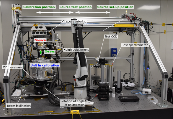
Figure 11: The instrument calibration equipment at INAF-IAPS. On the left a flight DU under calibration with a polarized source. At the center the Romer arm used for metrology is visible. On the right the CCD to study the beam image and the SDD to study the beam spectrum are just visible.

Table 4: The Crystals and the X-ray tubes used during GPD acceptance and DUs calibration. This is a subset of available energies. The column $\frac{R_{p}}{R_{s}}$ represents the ratio of the integrated reflectivity for polarization parallel and perpendicular to the crystal lattice plane at that given energy. From this ratio it is possible to derive the polarization degree of the reflected beam (from Henke et al. (1993))

Crystal	X-ray tube	Energy	2d	Diffraction	$\frac{R_{p}}{R_{s}}$	Polarization
		[keV]	$\AA$	Angle		[$\%$]
				[deg]
PET (002)	Continuum	2.01	8.742	45.0	0.0	$\approx$100.0
InSb (111)	Mo Lα	2.29	7.481	46.361	0.0034	99.2$\%$
Ge (111)	Rh Lα	2.7	6.532	44.877	0.00	$\approx$100.0
Si (111)	Ag Lα	2.98	6.271	41.562	0.0252	95.1$\%$
Al (111)	Ca $K_{\alpha}$	3.69	4.678	45.909	0.0031	99.4$\%$
Si (220)	Ti Kα	4.51	3.840	45.716	0.0023	99.5$\%$
Si (400)	Fe Kα	6.40	2.716	45.511		$\sim$ 100 $\%$

The calibration of the flight DUs was performed successfully following the on-ground calibration plan. The major effort was the calibration of the modulation factor and the characterization and the subtraction of spurious modulation at different energies. The detailed description of these features is the subject of forthcoming papers.

10 Instrument performance

We summarize here the instrument performances after calibration. We show in Figure 12 the results for spurious modulation and modulation factor. In the left panel we show spurious modulation re-phasing the modulation curves when considering a dispositions of the DUs as in flight (120^∘ clocking around Z-axis). The orientation of the DUs allows for reducing the spurious modulation of the instrument with respect to that of a single DU. Such spurious modulation is subtracted on event by event base. The right plot shows, instead, the modulation factor after keeping 80% of the data among the most elongated track and event-by-event spurious modulation subtraction.

Figure 12: a. Spurious modulation at instrument level (on a spot of 1.5 mm radius and combining the three DU’s clocked at 120^∘). b. Modulation factor of the instrument after spurious modulation subtraction (Average of the three DUs), with dithering on a flight-representative region of 1.5 mm radius.

In Table 5 we show the characteristics of the Instrument as average of the three DUs at two characteristic energies. These parameters can be considered as representative of the entire instrument. The detailed calibration results for each flight DU will be presented in a set of forthcoming papers.

Table 5: Instrument performance. Spurious modulation is effectively measured at instrument level, thus considering 120^∘ clocking of three DUs. Data are extracted in a circular region of 1.5 mm radius. Efficiency includes only the GPD contribution extrapolated at the time of the flight.

Parameter	2.69 keV	6.40 keV
Modulation factor	30.4 $\%$ $\pm$ 0.4 $\%$	56.6 $\%$ $\pm$ 0.4 $\%$
Efficiency (expected during flight)	13.5$\%$	1.7$\%$
Gray filter transparency	17.4 $\%$	88.0 $\%$
UV Filter transparency	(95.94 $\pm$ 0.26)$\%$	(99.44 $\pm$ 0.38) $\%$
Spurious modulation	(0.62 $\pm$0.05) $\%$	(0.29 $\pm 0.06$) $\%$ (@5.89 keV)
Systematic error on the P.A. determination	(0.143 $\pm$ 0.094)∘	(0.186 $\pm$ 0.097)∘
Energy resolution	(22.2$\pm$0.5)$\%$	(16.3$\pm$0.1)$\%$
Position resolution (HPD)	(118.7 $\pm$ 5.2) $\mu$m	120.0 $\pm$ 5.8) $\mu$m
Dead Time	1.1 ms	1.2 ms
Parameter	Value
Timing accuracy	1-2 $\mu$s (by means of the use of the PPS)
Timing resolution	1 $\mu$s
Common FoV	9’
Dithering radius	1’.6 standard (or 0’.8 or 2’.6 or no-dithering)
Expected background rate (2-8 keV)	1.9 10-3 c/s/cm2/keV
Expected Crab (nebula + pulsar) rate (2-8 keV)	150 c/s
Expected Crab (nebula + pulsar) rate (1-12 keV)	240 c/s

11 Processing Pipeline

Data are analyzed on ground. The first step of the pipeline is to convert binary telemetry files to FITS standard format by means of a parser. At this stage, data contain all the information provided by the Instrument and the relevant information from the spacecraft. In particular they contain the raw, pedestal-corrected, track images, the time of each count and all the relevant house-keeping like temperatures and event-by-event dead time. The FITS-converted data are then processed in order to transform the engineering unit in physical units, removing the non-necessary engineering information and including Good Time Interval information. The processing pipeline, then, uses calibration data in order to (1) equalize the pixel response of the track image; (2) identify by means of a clustering algorithm the photoelectron (principal) track; (3) estimate the emission direction in detector coordinates; (4) estimate the location of the events in detector coordinates; (5) estimate the energy of the track by applying (a) correction for charging, (b) correction for temperature and (c) GEM gain non-uniformities. The last step of the correction is the removal of spurious modulation, which is applied on the Stokes parameter calculated for each event. At this stage, track images are removed and data contain the position in detector coordinates, the time of the event, the energy of the event in “pulse invariant” unit, the emission direction in detector coordinates and the Stokes parameter of the event according to Kislat et al. (2015) definition with only an extra factor of 2. Next step is to merge the detector data from the three DUs, including their clocking at 120^∘, and to convert to celestial coordinates. The final event file to be used for science analysis, after that all the procedures are applied, contains all the information typical of imaging X-ray Astronomy mission, but with the addition of the information on the emission direction of the photoelectron in celestial coordinates.

12 Conclusion

We presented the instrument that was successfully designed, built, calibrated and installed in the spacecraft for the IXPE mission. These activities spanned 3.5 years, including phase B and the development time is compliant with readiness for a launch starting 17 November 2021. We reviewed the instrument design and the results of the calibration and we compared them with the ones expected on the basis of scientific astrophysical requirements. The modulation factor, the energy resolution, the position resolution of the instrument all meet the scientific requirements. The quantum efficiency is below requirement, but when factoring in all other parameters, the top level polarization sensitivity requirement is still met. Background also is expected to be slightly higher than the requirement (Xie et al., 2021). However, due to the relatively bright sources in the IXPE observing plan, we anticipate no effect in point-like sources observation and only a mild effect is expected in low surface brightness extended sources like the molecular clouds in the vicinity of the Galactic Center or in SN1006 supernova remnant. The calibration of the spare telescope, the only one to be calibrated, has been accomplished and its results will be part of a forthcoming paper. The preliminary results are such that in-flight performance of the IXPE payload will permit a new window to be opened in x-ray polarimetry.

References

- Angel et al. (1969) Angel, J. R., Novick, R., vanden Bout, P., & Wolff, R. 1969, Physical Review Letters, 22, 861, doi: 10.1103/PhysRevLett.22.861
- Baldini et al. (2021) Baldini, L., Barbanera, M., Bellazzini, R., et al. 2021, Astroparticle Physics (In Press)
- Barbanera et al. (2021) Barbanera, M., Citraro, S., Magazzu’, C., et al. 2021, IEEE Transactions on Nuclear Science, 1, doi: 10.1109/TNS.2021.3073662
- Bellazzini et al. (2006) Bellazzini, R., Spandre, G., Minuti, M., et al. 2006, Nuclear Instruments and Methods in Physics Research A, 566, 552, doi: 10.1016/j.nima.2006.07.036
- Bellazzini et al. (2007) Bellazzini, R., Spandre, G., Minuti, M., et al. 2007, Nuclear Instruments and Methods in Physics Research A, 579, 853, doi: 10.1016/j.nima.2007.05.304
- Black et al. (2007) Black, J. K., Baker, R. G., Deines-Jones, P., Hill, J. E., & Jahoda, K. 2007, Nuclear Instruments and Methods in Physics Research A, 581, 755, doi: 10.1016/j.nima.2007.08.144
- Connors & Stark (1977) Connors, P. A., & Stark, R. F. 1977, Nature, 269, 128, doi: 10.1038/269128a0
- Costa et al. (2001) Costa, E., Soffitta, P., Bellazzini, R., et al. 2001, Nature, 411, 662
- Elsner et al. (2012) Elsner, R. F., O’Dell, S. L., & Weisskopf, M. C. 2012, in Society of Photo-Optical Instrumentation Engineers (SPIE) Conference Series, Vol. 8443, doi: 10.1117/12.924889
- Fabiani et al. (2014) Fabiani, S., Costa, E., Del Monte, E., et al. 2014, ApJS, 212, 25, doi: 10.1088/0067-0049/212/2/25
- Feng et al. (2020) Feng, H., Li, H., Long, X., et al. 2020, arXiv e-prints, arXiv:2011.05487. https://arxiv.org/abs/2011.05487
- Ferrazzoli et al. (2020) Ferrazzoli, R., Muleri, F., Lefevre, C., et al. 2020, Journal of Astronomical Telescopes, Instruments, and Systems, 6, 048002, doi: 10.1117/1.JATIS.6.4.048002
- Heitler (1954) Heitler, W. 1954, Quantum theory of radiation (International Series of Monographs on Physics, Oxford: Clarendon, 1954, 3rd ed.)
- Henke et al. (1993) Henke, B. L., Gullikson, E. M., & Davis, J. C. 1993, Atomic Data and Nuclear Data Tables, 54, 181
- Hughes et al. (1984) Hughes, J. P., Long, K. S., & Novick, R. 1984, ApJ, 280, 255, doi: 10.1086/161992
- Kaaret et al. (1989) Kaaret, P., Novick, R., Martin, C., et al. 1989, in Society of Photo-Optical Instrumentation Engineers (SPIE) Conference Series, ed. R. B. Hoover, Vol. 1160, 587–597
- Kislat et al. (2015) Kislat, F., Clark, B., Beilicke, M., & Krawczynski, H. 2015, Astroparticle Physics, 68, 45, doi: 10.1016/j.astropartphys.2015.02.007
- La Monaca et al. (2021) La Monaca, F., Fabiani, S., Lefevre, C., et al. 2021, in Space Telescopes and Instrumentation 2020: Ultraviolet to Gamma Ray, ed. J.-W. A. den Herder, S. Nikzad, & K. Nakazawa, Vol. 11444 (SPIE), 1029–1039, doi: 10.1117/12.2567000
- Muleri et al. (2021) Muleri, F., Piazzolla, R., Di Marco, A., & et al. 2021, Astroparticle Physics (Submitted)
- Muleri et al. (2008a) Muleri, F., Soffitta, P., Baldini, L., et al. 2008a, Nuclear Instruments and Methods in Physics Research A, 584, 149, doi: 10.1016/j.nima.2007.09.046
- Muleri et al. (2008b) Muleri, F., Soffitta, P., Bellazzini, R., et al. 2008b, in Space Telescopes and Instrumentation 2008: Ultraviolet to Gamma Ray, ed. M. J. L. Turner & K. A. Flanagan, Vol. 7011, 701127, doi: 10.1117/12.789605
- Muleri et al. (2010) Muleri, F., Soffitta, P., Baldini, L., et al. 2010, Nuclear Instruments and Methods in Physics Research A, 620, 285, doi: 10.1016/j.nima.2010.03.006
- Novick et al. (1972) Novick, R., Weisskopf, M. C., Berthelsdorf, R., Linke, R., & Wolff, R. S. 1972, ApJ, 174, L1
- O’Dell et al. (2018) O’Dell, S. L., Baldini, L., Bellazzini, R., et al. 2018, in Society of Photo-Optical Instrumentation Engineers (SPIE) Conference Series, Vol. 10699, Space Telescopes and Instrumentation 2018: Ultraviolet to Gamma Ray, ed. J.-W. A. den Herder, S. Nikzad, & K. Nakazawa, 106991X, doi: 10.1117/12.2314146
- O’Dell et al. (2019) O’Dell, S. L., Attinà, P., Baldini, L., et al. 2019, in Society of Photo-Optical Instrumentation Engineers (SPIE) Conference Series, Vol. 11118, UV, X-Ray, and Gamma-Ray Space Instrumentation for Astronomy XXI, 111180V, doi: 10.1117/12.2530646
- Ramsey et al. (2019) Ramsey, B. D., Bongiorno, S. D., Kolodziejczak, J. J., et al. 2019, in Society of Photo-Optical Instrumentation Engineers (SPIE) Conference Series, Vol. 11119, Optics for EUV, X-Ray, and Gamma-Ray Astronomy IX, 1111903, doi: 10.1117/12.2531956
- Sanford et al. (1970) Sanford, P. W., Cruise, A. M., & Culhane, J. L. 1970, in Non-Solar X- and Gamma-Ray Astronomy, ed. L. Gratton, Vol. 37, 35
- Schnopper & Kalata (1969) Schnopper, H. W., & Kalata, K. 1969, AJ, 74, 854, doi: 10.1086/110873
- Soffitta et al. (1998) Soffitta, P., Costa, E., Kaaret, P., et al. 1998, Nuclear Instruments and Methods in Physics Research A, 414, 218, doi: 10.1016/S0168-9002(98)00572-5
- Soffitta & XIPE Collaboration (2017) Soffitta, P., & XIPE Collaboration. 2017, Nuclear Instruments and Methods in Physics Research A, 873, 21, doi: 10.1016/j.nima.2017.02.025
- Soffitta et al. (2001) Soffitta, P., Costa, E., di Persio, G., et al. 2001, Nuclear Instruments and Methods in Physics Research A, 469, 164, doi: 10.1016/S0168-9002(01)00772-0
- Soffitta et al. (2012) Soffitta, P., Campana, R., Costa, E., et al. 2012, in Society of Photo-Optical Instrumentation Engineers (SPIE) Conference Series, Vol. 8443, Society of Photo-Optical Instrumentation Engineers (SPIE) Conference Series, doi: 10.1117/12.925385
- Soffitta et al. (2013a) Soffitta, P., Muleri, F., Fabiani, S., et al. 2013a, Nuclear Instruments and Methods in Physics Research A, 700, 99, doi: 10.1016/j.nima.2012.09.055
- Soffitta et al. (2013b) Soffitta, P., Barcons, X., Bellazzini, R., et al. 2013b, Experimental Astronomy, 36, 523, doi: 10.1007/s10686-013-9344-3
- Soffitta et al. (2020) Soffitta, P., Attinà, P., Baldini, L., et al. 2020, in Society of Photo-Optical Instrumentation Engineers (SPIE) Conference Series, Vol. 11444, Society of Photo-Optical Instrumentation Engineers (SPIE) Conference Series, 1144462, doi: 10.1117/12.2567001
- Stark & Connors (1977) Stark, R. F., & Connors, P. A. 1977, Nature, 266, 429
- Swank (2010) Swank, J. e. a. 2010, in X-ray Polarimetry: A New Window in Astrophysics by Ronaldo Bellazzini, Enrico Costa, Giorgio Matt and Gianpiero Tagliaferri. Cambridge University Press, 2010. ISBN: 9780521191845, p. 251, ed. R. Bellazzini, E. Costa, G. Matt, & G. Tagliaferri, 251
- Tamagawa & et al. (2010) Tamagawa, T., & et al. 2010, Ideal gas electron multipliers (GEMs) for X-ray polarimeters, ed. R. Bellazzini, E. Costa, G. Matt, & G. Tagliaferri, 60
- Tamagawa et al. (2009) Tamagawa, T., Hayato, A., Asami, F., et al. 2009, Nuclear Instruments and Methods in Physics Research A, 608, 390, doi: 10.1016/j.nima.2009.07.014
- Tomsick et al. (1997) Tomsick, J., Costa, E., Dwyer, J., et al. 1997, in Society of Photo-Optical Instrumentation Engineers (SPIE) Conference Series, Vol. 3114, Society of Photo-Optical Instrumentation Engineers (SPIE) Conference Series, ed. O. H. Siegmund & M. A. Gummin, 373–383
- Weisskopf et al. (1978a) Weisskopf, M. C., Kestenbaum, H. L., Long, K. S., Novick, R., & Silver, E. H. 1978a, ApJ, 221, L13, doi: 10.1086/182655
- Weisskopf et al. (1978b) Weisskopf, M. C., Silver, E. H., Kestenbaum, H. L., Long, K. S., & Novick, R. 1978b, ApJ, 220, L117, doi: 10.1086/182648
- Weisskopf et al. (1977) Weisskopf, M. C., Silver, E. H., Kestenbaum, H. L., et al. 1977, ApJ, 215, L65, doi: 10.1086/182479
- Weisskopf et al. (2008) Weisskopf, M. C., Bellazzini, R., Costa, E., et al. 2008, in Society of Photo-Optical Instrumentation Engineers (SPIE) Conference Series, Vol. 7011, Society of Photo-Optical Instrumentation Engineers (SPIE) Conference Series, doi: 10.1117/12.788184
- Weisskopf et al. (2016) Weisskopf, M. C., Ramsey, B., O’Dell, S., et al. 2016, in Society of Photo-Optical Instrumentation Engineers (SPIE) Conference Series, Vol. 9905, Space Telescopes and Instrumentation 2016: Ultraviolet to Gamma Ray, ed. J.-W. A. den Herder, T. Takahashi, & M. Bautz, 990517, doi: 10.1117/12.2235240
- Xie et al. (2021) Xie, F., Ferrazzoli, R., Soffitta, P., et al. 2021, Astroparticle Physics, 128, 102566, doi: 10.1016/j.astropartphys.2021.102566
- Zombeck (2007) Zombeck, M. 2007, Handbook of Space Astronomy and Astrophysics: Third Edition