Multivariate -normal distributions
Krzysztof Zajkowski
Faculty of Mathematics, University of Bialystok
Ciolkowskiego 1M, 15-245 Bialystok, Poland
kryza@math.uwb.edu.pl
Abstract
The Weibull distribution can be obtained using a power transformation from the standard exponential distribution. In this article, we will consider a symmetrized power transformation of a random variable with the standard normal distribution. We will call its distribution the -normal (Gaussian) distribution. We examine properties of this distribution in detail. We calculate moments and consider the moment problem of -normal distribution. We derive the formula of its differential entropy and (exponential) Orlicz norm. Moreover, we define the joint distribution function of the multivariate -normal distribution as a meta-Gaussian distribution with -normal marginals. We consider also the limiting distribution as tends to infinity.
2020 Mathematics Subject Classification: Primary 60E05, Secondary 46E30.
Key words: normal distribution, Weibull distribution, differential entropy, sub-exponential random variables, (exponential) Orlicz norms, copulas, meta-Gaussian distributions
1 Introduction
The Weibull distribution is one of the most important and well-known probability distributions, which has a wide range of applications (see, e.g., Rinne’s extensive monograph [11]). The Weibull distribution can be obtained from the standard exponential distribution by power transformation (see Johnson, Kotz and Balakrishnan [5, Ch.8]), i.e., if has the exponential distribution with parameter then () has two-parameter Weibull distribution with the shape parameter and the scale parameter . The random variable (r.v.) has -exponential tail decay and belongs to the corresponding exponential type Orlicz space (see Section 4).
In this article, we propose applying a power transformation of the form to a random variable with the standard normal distribution to obtain some equivalent to the Weibull random variable. This variable will have the same order of tail decay and will belong to the same Orlicz space as the variable .
A multivariate Weibull distribution can in general be obtained from multivariate exponential distribution by power transformations of marginals (see Kotz, Balakrishnan and Johnson [6, Ch. 47.4], i.e., if have some joint exponential distribution then the power transformations produce a multivariate distribution having Weibull marginals. There are many forms of multivariate exponential distributions. In general it depends on copulas used (see [6, Ch. 47]). In this paper, we apply the particular Gauss copula to the -normal marginals. We call this probability distribution a multivariate -normal distribution. In other words, we define this distribution as a meta-Gaussian distribution with -normal marginals. We consider also the limiting distribution as tends to infinity.
2 The -normal distribution
We define a power transformation of the normal distribution, which was announced in [13].
Definition 2.1.
Let be the standard normal distributed random variable and be a positive number. We denote by the random variable , where is the signum function of . We call the model -normal (-Gaussian) random variable.
Remark 2.2.
Let us emphasize that . is the standard normally distributed random variable. All results that we obtain for are generalizations known facts for the normal distribution.
Remark 2.3.
Since the function is odd and is a symmetric random variable, is the symmetric one and has the same distribution as .
Remark 2.4.
Tails of the Gaussian random variable can be estimated from above in the following way
for any ; see, for instance, [2, Prop.2.2.1]). Hence for -normal random variable we get
This means that has the -sub-exponential tails decay.
Proposition 2.5.
i) The distribution function (d.f.) of is of the form
where is the standard normal distribution function.
ii) The probability density function of is of the form
Proof.
Let us observe that is bijection and its inverse is of the form . Thus the distribution function of the -Gaussian random variable , which we will denote by , has the form
For the second part, since
we infer that the density function has the form as in the assertion. ∎
Density function description (The following description and the graphic were made by the student Jacek Oszczepaliński).
The density function of the random variable is an even function. If we consider , the derivative of this function has the following expression
It is worth noting that for , the density function exhibits an infinite negative slope at (i.e., ), and it is negative for all . In the case of , the slope at is finite, and we have . For , the slope at is infinitely positive, and when , we have , while for . In general, for and , the slope of the density function is positive up to the value , where , and it is negative beyond the aforementioned threshold.
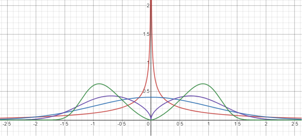
The shape of the density function of the standard -normal distribution undergoes a significant transformation depending on the value of . Specifically, for values within the range of , the function exhibits a vertical asymptote at zero. When equals , the function describes the density of a standard normal distribution. However, for , the function features a local minimum at zero with a value of zero and two maxima at , depicting a distinct bimodal distribution.
The figure below displays graphs of -normal probability density functions, each with different values of the shape parameter . Specifically, the density functions represented by the colours red, blue, purple, and green correspond to values of , , , and , respectively.
Remark 2.6.
Remark 2.7.
Let us observe that for each the distribution function tends weakly to the Rademacher distribution as . For this reason we will denote the Rademacher distribution by .
The moment problem of -normal distribution. Since, for and ,
we immediately get
Let us emphasize that and its modulus both have finite integer-order moments. It is natural to ask about the moment problem (see Stoyanov [12, Sec.11] for instance). That is, let
we ask whether is uniquely determined (-determinate) or indetermined (-indeterminate) by the sequence of moments . Following Stoyanov’s reasoning from [12, Subsection 11.1], we can answer this question (the necessary definitions and criteria can be found at the beginning of [12, Section 11]).
Stoyanov considers the random variable in detail, writing that all odd powers of can be considered in a similar way. Note that with our parametrization () and in general (). Let us emphasize that the presented reasoning is true for any .
By using some standard integrals (, and , ) we conclude that
Hence, according to the Krein criterion (see () in [12, Sec.11] for instance) the distribution of r.v. is -indeterminate for .
Now we prove that for the d.f. of is -determinate. To simplify the notation we write if , where is a positive constant, which depends only on . Let us note that
and
for sufficiently large (e.g. ). By Stirling’s formula
Since if , we get that
for . By Carleman’s condition (see in [12, Sec.11]) we obtain that is -determinate for .
Moreover one can calculate that the moment generating function (m.g.f.) of takes the form for . Thus we can deduce that has light tails for (possesses the m.g.f.).
Remark 2.8.
Repeating the above reasoning for the random variable and using Krein’s and Carleman’s conditions for its probability distribution with the support , one can calculate that is -indeterminate for and -determinate for , although has the m.g.f. only from (compare the example in [12, Sec.11.1]).
3 Comparison with the Weibull distribution
Now we compare the distribution of with the distributions of the Weibull() random variables for some ’s. By definition, a random variable majorizes a random variable in distribution, if there exists such that
for any ; see, for instance, [1, Def. 1.1.2].
Proposition 3.1.
The -normal random variable majorizes the Weibull(,1) random variable and it is majorized by the Weibull() random variable.
Proof.
It is known that the tails of the Gaussian random variable can be estimated from above in the following way
for any ; see, for instance, [2, Prop.2.2.1]) . Hence for the -normal random variable we get
| (1) |
Observe that the right hand side is a tail of the Weibull() random variable. This means that the Weibull() random variable majorizes the -normal random variable.
In the same source [2, Prop.2.2.1]) one can find the following lower estimate of the tails of the Gaussian random variable
for . Since tends to as , there exists such that for . It gives and, in consequence,
for . By the above
for , which means that the -normal random variable majorizes the Weibull() random variable. ∎
Although the model -normal distribution is comparable to the Weibull distribution in the above sense, it is significantly different. We show it using the entropy function. Recall that the differential entropy of the two-parameter Weibull distribution is given by the formula
where is the Euler-Mascheroni constant. For this is distinct.
Proposition 3.2.
The differential entropy of has the following form
where denotes the Euler-Mascheroni constant.
Proof.
For we get the differential entropy of the standard Gaussian variable .
4 Orlicz norm of the -normal distribution
Let us emphasize that Weibull random variables are the model examples of random variables with -sub-exponential tail decay. We say that a random variable has the -sub-exponential tail decay if there exist two constant such that for it holds
Since
the Weibull random has -sub-exponential tail decay with and . Whereas the estimate (1) means that has such a tail decay with and .
The property of -sub-exponential tail decay can be equivalently expressed in terms of so-called (exponential) Orlicz norms. Recall that for any random variable , -norm is defined by
according to the standard convention . We call the above functional -norm but let us emphasize that only for it is a proper norm. For it is quasi-norm. It does not satisfy the triangle inequality (see Appendix A in [3] for more details). One can observe that and, moreover, one can check that, for , ; see Lemma 2.3 in [13].
Since the closed form of the moment generating function of random variable is known, we can calculate the -norm of -normal random variable . Since has -distribution with one degree of freedom whose moment generating function is for , we get
which is less or equal if . It gives that . The -norm of is equal to -norm of . By Lemma 2.3 in [13] and the definition of -normal distribution we get
Remark 4.1.
Using the closed form of the moment generating function of the standard exponential random variable and the above mentioned definition of the two-parameter Weibull distribution, similarly as for the standard -Gaussian random variable, one can obtain its -norm .
Remark 4.2.
Although the Weibull() random variables provide model examples of random variables with -sub-exponential tail decay (they are model elements of spaces generated by the -norms), it can nevertheless be argued that the -Gaussian variables should play a central role among these variables (in these spaces).
5 Multivariate -normal distributions
We define the multivariate -normal distribution as the meta-Gaussian distribution with -normal margins, i.e., as a composition of the Gauss copula with the -normal distributions. Recall that the Gauss copula with the correlation matrix is defined as
where is the d.f. of distribution; see [7, (5.9)] for instance.
Definition 5.1.
We define the joint distribution function of the multivariate -normal distribution as
Proposition 5.2.
i) The joint distribution function of the multivariate -normal distribution is of the form
ii) The density function of the multivariate -normal distribution is
where is the density function of distribution.
Proof.
By the form of and Proposition 2.5 we get forms of the multivariate -normal distribution and its density function, i.e.,
and, for the second part,
∎
Example 5.3.
Recall that the standard bivariate normal density function with the correlation coefficient is of the form
By the above proposition, the bivariate -normal density function with the coefficient takes the form
6 Limiting distribution
The Gauss copula is a continuous function. Taking into account Remark 2.7 we get the weak convergence of the multivariate -normal distribution to the meta-Gaussian distribution with Rademacher’s margins as . This limiting distribution we denote by . Thus
Let be a random vector with the cdf . Then is a discrete random vector with . We recall the notation for counting elements in lexicographic order. For any vectors and , we denote by the number of indices for which , i.e.,
By the inclusion-exclusion principle and the form of we immediately get the following form of the probability mass function of .
Proposition 6.1.
Let be a random vector with the distribution function . Then the probability mass function at is given by
where denotes the lexicographic order on .
Example 6.2.
Let a random vector has the cdf , where is a correlation coefficient of the Gauss copula . Then
Let us note that takes only three values: , and . By the definition of a copula and using its Frechet bounds we have
and
The probability mass function of is concentrated at points , , and . Successively we get
Similarly
and finally
Summarizing
and
References
- [1] V. Buldygin, Yu. Kozachenko, Metric Characterization of Random Variables and Random Processes, Amer.Math.Soc., Providence, 2000.
- [2] R.M. Dudley, Uniform Central Limit Theorems, Cambridge University Press, 1999.
- [3] F. Götze, H. Sambale, A. Sinulis (2021) Concentration inequalities for polynomials in -sub-exponential random variables, Electron. J. Probab. 26, article no. 48, 1-22.
- [4] I.S. Gradshteyn, I.M. Ryzhik, Table of Integrals, Series, and Products, Seventh Edition, Academic Press, 2007.
- [5] N.L. Johnson, S. Kotz, N. Balakrishnan, Continuous Univariate Distributions, Vol. 1, Wiley Series in Probability and Mathematical Statistics: Applied Probability and Statistics (2nd ed.), New York: John Wiley & Sons, 1994.
- [6] Kotz, S.,N. Balakrishnan, Norman L. Johnson Continuous multivariate distributions : Volume 1: models and applications 2nd ed., 2000
- [7] Alexander J. McNeil, Rudiger Frey and Paul Embrechts (2005), Q͡uantitative Risk Management: Concepts, Techniques, and Tools, Princeton Series in Finance.
- [8] D. Li (2000), On default correlation: A copula function approach, The Journal of Fixed Income, 9(4):43-54,
- [9] B. Renard, M. Lang. (2007), Use of a Gaussian copula for multivariate extreme value analysis: some case studies in hydrology, Advances in Water Resources, 30, 897-912.
- [10] Rey, M., Roth, V. (2012). Meta-Gaussian information Bottleneck, Advances in Neural Information Processing systems, INIPS: San Diego, CA, USA, pp.1916-1924.
- [11] H. Rinne, The Weibull Distribution, Taylor & Francis Group, 2009
- [12] J. Stoyanov, Counterexamples in Probability, 3rd rev. ed., Dover Publications, Mineola, NY, 2013.
- [13] K. Zajkowski (2020) Concentration of norms of random vectors with independent -sub-exponential coordinates, arXiv:1909.06776.