RLTutor: Reinforcement Learning Based Adaptive Tutoring System
by Modeling Virtual Student with Fewer Interactions

Abstract

A major challenge in the field of education is providing review schedules that present learned items at appropriate intervals to each student so that memory is retained over time. In recent years, attempts have been made to formulate item reviews as sequential decision-making problems to realize adaptive instruction based on the knowledge state of students. It has been reported previously that reinforcement learning can help realize mathematical models of students learning strategies to maintain a high memory rate. However, optimization using reinforcement learning requires a large number of interactions, and thus it cannot be applied directly to actual students. In this study, we propose a framework for optimizing teaching strategies by constructing a virtual model of the student while minimizing the interaction with the actual teaching target. In addition, we conducted an experiment considering actual instructions using the mathematical model and confirmed that the model performance is comparable to that of conventional teaching methods. Our framework can directly substitute mathematical models used in experiments with human students, and our results can serve as a buffer between theoretical instructional optimization and practical applications in e-learning systems.

1 Introduction

The demand for online education is increasing as schools around the world are forced to close due to the COVID-19 pandemic. E-learning systems that support self-study are gaining rapid popularity. While e-learning systems are advantageous in that students can study from anywhere without gathering, they also have the disadvantage of making it difficult to provide an individualized curriculum, owing to the lack of communication between teachers and students Zounek and Sudicky (2013).

Instructions suited to individual learning tendencies and memory characteristics have been investigated recently Pavlik and Anderson (2008); Khajah et al. (2014). Flashcard-style questions, where the answer to a question is uniquely determined, have attracted significant research attention. Knowledge tracing Corbett and Anderson (1994) aims to estimate the knowledge state of students based on their learning history and uses it for instruction. In this context, it has been reported that the success or failure of future students’ answers can be accurately estimated using psychological findings Lindsey et al. (2014); Choffin et al. (2019) and deep neural networks (DNNs) Piech et al. (2015).

Furthermore, adaptive instructional acquisition has also been formulated as a continuous decision problem to optimize the instructional method Rafferty et al. (2016); Whitehill and Movellan (2017); Reddy et al. (2017); Utkarsh et al. (2018). Reddy et al. Reddy et al. (2017) considered the optimization of student instruction as an interaction between the environment (students) and the agent (teacher), and they attempted to optimize the instruction using reinforcement learning. Although their results outperform existing heuristic teaching methods for mathematically modelled students, there is a practical problem in that it cannot be applied directly to actual students. This is because of the extremely large number of interactions required for optimization.

In this study, we propose a framework that can optimize the teaching method while reducing the number of interactions between the environment (modeled students) and the agent (teacher) using a pretrained mathematical model of the students. Our contributions are summarized as follows.

• We pretrained a mathematical model that imitates students using mass data, and realized adaptive instruction using existing reinforcement learning with a smaller number of interactions.

• We conducted an evaluation experiment of the proposed framework in a more practical setting, and showed that it can achieve comparable performance to existing methods with fewer interactions.

• We highlighted the need to reconsider the functional form of the loss function for the modeled students to realize more adaptive instruction.

2 Related Work

2.1 Knowledge Tracing

Knowledge tracing (KT) Corbett and Anderson (1994) is a task used to estimate the time-varying knowledge state of learners from the corresponding learning histories. Various methods have been proposed for KT, including those using Bayesian estimation Michael et al. (2013), and DNN-based methods Piech et al. (2015); Pandey and Karypis (2019).

In this study, we focus on the item response theory (IRT) Frederic (1952). IRT is aimed at evaluating tests that are independent of individual abilities. The following is the simplest logistic model:

$$\mathbb{P}\lparen O_{i,j}=1\rparen=\sigma\lparen\alpha_{i}-\delta_{j}\rparen.$$ (1)

Here, $\alpha_{i}$ is the ability of the learner $i$, $\delta_{j}$ is the difficulty of the question $j$, and $O_{i,j}$ is a random variable representing the correctness $o$ of learner $i$’s answer to question $j$ in binary form. $\sigma\lparen\cdot\rparen$ represents the sigmoid function. While ordinary IRT is a static model with no time variation, IRT-based KT attempts to realize KT by incorporating learning history into Equation (1) Cen et al. (2006); Pavlik et al. (2009); Vie and Kashima (2019). Lindsey et al. Lindsey et al. (2014) proposed the DASH model, which uses psychological knowledge to design a history parameter. Since DASH does not consider the case where multiple pieces of knowledge are associated with a single item, Choffin et al. Choffin et al. (2019) extended DASH to consider correlations between items, and the model is called DAS3H:

$$\mathbb{P}\lparen O_{i,j,l}=1\rparen$$

$$=\sigma\Bigl{\lparen}\alpha_{i}-\delta_{j}+\displaystyle\sum_{k\in\mathrm{KC}_{j}}{\beta_{k}}+h_{\theta,\phi}\lparen t_{i,j,1:l},o_{i,j,1:l-1}\rparen\Bigl{\rparen},$$ (2)

$$h_{\theta,\phi}\lparen t_{i,j,1:l},o_{i,j,1:l-1}\rparen$$

$$=\sum_{k\in\mathrm{KC}_{j}}\sum_{w=0}^{W-1}{\theta_{k,w}\ln\lparen 1+c_{i,k,w}\rparen+\phi_{k,w}\ln\lparen 1+n_{i,k,w}\rparen.}$$ (3)

Equation (2) contains two additional terms from Equation (1): the proficiency $\beta_{k}$ of the knowledge components (KC) associated with item $j$, and $h_{\theta,\phi}$ defined in Equation (3). $h_{\theta,\phi}$ represents students’ learning history, $n_{i,k,w}$ refers to the number of times learner $i$ attempts to answer skill $k$, and $c_{i,k,w}$ refers to the number of correct answers out of the trials, both counted in each time window $\tau_{w}$. Time window $\tau_{w}$ is a parameter that originates from the field of psychology Rovee-Collier (1995), and represents the time scale of loss of memory. By dividing the counts by each discrete time scale satisfying $\tau_{w}<\tau_{w+1}$, the memory rate can be estimated by taking into account the temporal distribution of the learning history Lindsey et al. (2014).

2.2 Adaptive Instruction

A mainstream approach to adaptive instruction is the optimization of review intervals. The effects of repetitive learning on memory consolidation have been discussed in the field of psychology Ebbinghaus (1885), and various studies have experimentally confirmed that gradually increasing the repetition interval is effective for memory retention Leitner (1974); Wickelgren (1974); Landauer and Bjork (1978); Wixted and Carpenter (2007); Cepeda et al. (2008).

Previously, the repetition interval was determined algorithmically when the item was presented Khajah et al. (2014). However, in recent years, there have been some attempts to obtain more personalized instruction by treating such instruction as a sequential decision problem Rafferty et al. (2016); Whitehill and Movellan (2017); Reddy et al. (2017); Utkarsh et al. (2018). Rafferty et al. Rafferty et al. (2016) formulated student instruction as a partially observed Markov decision process (POMDP) and attempted to optimize instruction for real students through planning for multiple modelled students. Based on their formulation, Reddy et al. Reddy et al. (2017) have also attempted to optimize instructional strategies using trust region policy optimization (TRPO) Schulman et al. (2015), a method of policy-based reinforcement learning. However, optimization by reinforcement learning requires a large number of interactions, which makes it inapplicable to real-life scenarios.

3 Proposed Framework

To address the issue of large numbers of interactions, we formulate a framework for acquiring adaptive instruction with fewer contacts. In this section, we consider student teaching as a POMDP and formulate a framework for acquiring adaptive teaching with a small number of interactions.

The proposed method has two main structures: a memory model that captures the knowledge state of the student (inner model) and a teaching model that acquires the optimal instructional strategy through reinforcement learning (RLTutor). As shown in Figure 1, RLTutor optimizes its strategy indirectly through interaction with the inner model, rather than with the actual student. In the following sections, we first describe the detailed design of the inner model and RLTutor and describe the working principle of our framework.

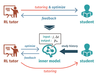
Figure 1: Illustration of the difference between the usual reinforcement learning setting and the proposed method. The proposed method updates the instructional strategies not by interacting with the students directly, but by interacting with the KT model estimated from the student’s study history.

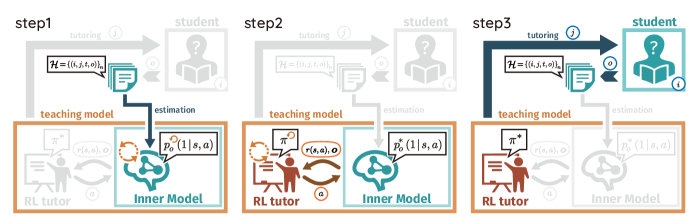
Figure 2: Graphical representation of each step of the proposed framework. First, the Inner Model is updated from the learning history of the student. Next, RLTutor optimizes the teaching policies for the updated Inner Model. Finally, RLTutor presents items to the target based on the optimized policy. Before the start of the experiment, the Inner Model is pretrained using the educational dataset, and then updated by minimizing the loss function in Equation (11) using all the historical data obtained up to that point.

3.1 Inner Model

Inner Model is a virtual student model constructed from the learning history of the instructional target using the KT method described in Section 2.1. Specifically, given a learning history $\mathcal{H}=\{i,j,t,o\}_{n}$ with the same notation as in Section 2.1, the model returns the probability of the correct answer $p_{o}$ for the next given question. In this study, we adopted the DAS3H model expressed in Equations (2) and (3) as the KT method. However, because this model uses a discrete time window to account for past learning, the estimated memory probability may vary from $1$, even if the same item is presented consecutively (e.g., without an interval). However, the human brain is capable of remembering meaningless symbols for a few seconds to a minute Miller (1956). To capture this sensory memory, we adopted the functional form proposed by Wicklegren Wickelgren (1974) and used:

$$p_{o}\left\lparen O=1\mid s,a\right\rparen\coloneqq\lparen 1-p_{D}\rparen\lparen 1+h\cdot\Delta t\rparen^{-f}+p_{D}$$ (4)

as the equation for the internal model with $p_{\mathrm{D}}$ Choffin et al.’s DAS3H model. In this study, $h$ and $f$ in Equation (4) are regarded as constants, and set to $h=0.3,f=0.7$. This is because individual differences in sensory memory are much smaller than those in long-term memory.

3.2 RLTutor

RLTutor is an agent that learns an optimal strategy $\pi^{*}$ using reinforcement learning based on the responses from the inner model, and uses the obtained strategy to provide suboptimal instruction to actual students.

As for the POMDP formulation, we assume that the true state $\mathcal{S}=\mathbb{R}^{I\times J\times K\times(W\times K)^{2}}\times{\mathbb{N}_{0}}^{(I\times K\times W)^{2}}$ of the student is not available, and only the correct and incorrect responses of the student can be obtained as an observation $\mathcal{O}=\{0,1\}$. We also set the immediate reward $r(s,a)$ as the average of the logarithmic memory retention for all problems at that time:

$$r(s,a)=\displaystyle\frac{1}{J}\sum_{j=1}^{J}\log p_{o}\left\lparen O_{j}=1\mid s,a\right\rparen.\\$$ (5)

For the above partial observation problem, we applied the proximal policy optimization (PPO) Schulman et al. (2017) method, which is a derivation of the TRPO. The policy function $\pi(a|s)$ is comprised of a neural network, including a gated recurrent unit (GRU) with 512 hidden layers.

Following Reddy et al. Reddy et al. (2017) we defined the input to the network as:

$$\bm{o} =\begin{pmatrix}\bm{j}_{\mathrm{e}}\\ \bm{t}_{\mathrm{e}}\\ o\end{pmatrix}\in\mathbb{R}^{\log{2J}+2+1},$$ (6)

where $\bm{j}_{\mathrm{e}}$ is a vector embedded with the presented item number $j$ following Equation (7) – (9), $\bm{t}_{\mathrm{e}}$ is a vector embedded with the time elapsed since the previous interaction $\Delta t$ following Equation (10), and $o$ is the student’s response:

$$\bm{v}_{1} =\text{onehot}(j)\in\mathbb{R}^{J},$$ (7)

$$\bm{v}_{2} =\begin{pmatrix}\bm{v}_{1}\cdot(1-o)\\ \bm{v}_{1}\cdot o\end{pmatrix}\in\mathbb{R}^{2J},$$ (8)

$$\bm{j}_{\mathrm{e}} =g(\bm{v}_{2})\in\mathbb{R}^{\log{2J}},$$ (9)

$$\bm{j}_{\mathrm{t}} =\begin{pmatrix}\log{\Delta t}\cdot(1-o)\\ \log{\Delta t}\cdot o\end{pmatrix}\in\mathbb{R}^{2}.$$ (10)

Note that $g$ is a random projection function ($\mathbb{R}^{2J}\rightarrow\mathbb{R}^{\log{2J}}$), compressing the sparse one-hot vector to a lower dimension without loss of information Piech et al. (2015).

3.3 Working Principle

Based on the two components described above, the proposed framework operates by repeating the following three steps (Figure 2).

1. Estimation: The inner model is updated based on students’ learning history.

2. Optimization: RLTutor optimizes the strategy for the updated inner model.

3. Instruction: RLTutor poses an item to the student using the current strategy.

Because it is difficult to train the inner model from scratch, we pretrained it using EdNet, which is the largest existing educational dataset Youngduck et al. (2020). We trained DAS3H on this dataset and determined the initial values of the Inner Model’s weights from the distribution of the estimated parameters. For details, please see the code to be released soon. In addition, in step 1, we used the following loss function to prevent excessive deviation from the pre-trained weights:

$$\mathcal{L}=\mathcal{L}^{\mathrm{MSE}}+\displaystyle\sum_{m}c_{m}\{\lparen 1-\lambda\rparen\mathcal{L}_{m}^{\mathrm{DIST}}+\lambda\mathcal{L}_{m}^{\mathrm{FIX}}\}.\\$$ (11)

Here, $\mathcal{L}^{\mathrm{MSE}}$ is introduced to make the output $p_{o}$ of the model closer to the student’s response $o$ obtained as the study history. $\mathcal{L}_{m}^{\mathrm{DIST}}$ and $\mathcal{L}_{m}^{\mathrm{FIX}}$ are constraint terms that prevent each parameter of the model from deviating from the distribution obtained in the prior training and from the value of the previous parameter, respectively. These can be expressed as:

$$\mathcal{L}^{\mathrm{MSE}} \coloneqq\displaystyle\sum_{n}\bigl{\lparen}o-p_{o}\bigr{\rparen}^{2},$$ (12)

$$\mathcal{L}_{m}^{\mathrm{DIST}} \coloneqq\displaystyle\sum_{n}\left\lparen 1-\frac{f_{m}\lparen\rho_{m}\rparen}{f_{m}\lparen\mu_{m}\rparen}\right\rparen,$$ (13)

$$\mathcal{L}_{m}^{\mathrm{FIX}} \coloneqq\displaystyle\sum_{n}|\rho_{m}-\grave{\rho}_{m}|,$$ (14)

where $f_{m}(x)$ is the normal distribution with mean $\mu_{m}$ and variance $\sigma_{m}$, both of which are obtained during pretraining. $\rho_{m}$ is a generalized representation of each parameter of the DAS3H model($\rho_{1}=\alpha,\rho_{2}=\delta,\rho_{3}=\beta,\rho_{4}=\theta,\rho_{5}=\phi$).

In this manner, we attempted to obtain adaptive instruction while reducing the number of interactions with the teaching target.

4 Experiment

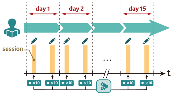
Figure 3: Experimental flow. Students who are substituted in the mathematical model are required to study a total of 30 items through 15 days. There are two intensive learning periods (called “sessions”) per day, and the teacher agents present 10 items for each session.

Figure 4: Diagrammatic representation of the plotting mechanism. The mathematical model used on behalf of the students can calculate the memory rate for each item at each step. First, an average over all items is evaluated. Because the responses to the items have been recorded 300 times (30 sessions with 10 items in each session), we then plot the mean values over each session.

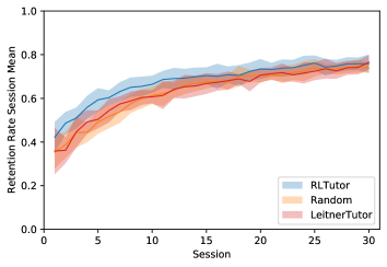
(a) VS LeitnerTutor

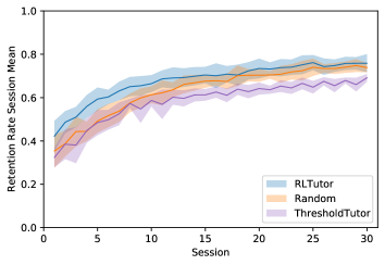
(b) VS ThresholdTutor

Figure 5: Plot of experimental results. We compare LeitnerTutor in Figure 5 and ThresholdTutor in Figure 5, in addition to RandomTutor and RLTutor.

To verify the effectiveness of the proposed framework, we conducted a comparison experiment with other instructional methods: RandomTutor, LeitnerTutor, ThresholdTutor, and RLTutor. RandomTutor is a teacher that presents problems completely randomly. LeitnerTutor is a teacher that presents problems according to the Leitner system, which is a typical interval iteration method. ThresholdTutor is a teacher that presents problems based on the student’s memory rate closest to a certain threshold value. Since user testing with actual students is costly, the mathematical model (DAS3H model) was used for the students taught in this experiment.

The experimental setup was such that the learner had to study 30 items in 15 days. To make the setting more realistic, we set up two sessions per day to study the items intensively, each session presenting 10 items. Figure 3 illustrates the outline of the experiment.

The Inner Model was updated for each session using a batch of all the previous historical data, and it was trained for 10 epochs. Note that the coefficients $c_{m}$ of the constraint terms of the loss function in Equation (4) were all set to one. For PPO training, mini-batches of size 200 were created every 4000 steps, and 20 agents were trained in parallel for 10 epochs. For the hyperparameters, we set the clipping parameter to 0.2, the value function coefficient to 0.5, the entropy coefficient to 0.01, the generalized advantage estimator (GAE) parameter to 0.95, and the reward discount rate to 0.85. The initial learning rate for all parameters was 0.5. In both cases, we used the Adam optimizer with an initial learning rate of 0.0001, which was gradually reduced to zero every two sessions.

The results of the experiments are shown in Figures 5 and  5. Figure 5 shows the results of instruction by RLTutor and LeitnerTutor, and Figure 5 shows the results of instruction by RLTutor and ThresholdTutor. The experiments were conducted five times with different seed values, and we plotted the average of the students’ memory rates over items and sessions. The solid lines represent the mean values, and the colored bands represent the standard deviations. To aid comprehension, we illustrate how the item-session average is calculated in Figure 4. Figure 5 shows that retention was strengthened in both methods of instruction. The figure shows that the instruction by the proposed method successfully maintains a higher memory rate than the other methods. In addition, the instruction by ThresholdTutor did not maintain the memory rate of the students as well as other methods. However, as the sessions continued, the performance of our method decreased. The reasons for these results will be discussed in the Discussion section.

5 Discussion

5.1 Why are there not much differences?

There are three possible reasons for why all the methods improved the students’ memory rate with approximately similar results: the experimental setup, loss function of the Inner Model, and gap between the model and the actual students.

5.1.1 Experimental Setup

The first reason is the experimental setup. In this experiment, we set a relatively long learning period (15 days) for a small number of questions (30 questions). Therefore, all questions would have been learned sufficiently, regardless of how they were presented. This leads to similar final memory rates for all methods.

5.1.2 Inner Model’s Loss Function

The next reason is the invariance of the Inner Model. As shown in Equation (4), a constraint term was added to the loss function of the Inner Model to avoid any deviation from the pre-learned weights and from the weights learned in the previous sessions. It is possible that these constraints are significantly strong, and that the Inner Model was not “fine-tuned” as the experiment progressed.

5.1.3 Gap between Model and the Actual Students

The last possible reason is the accuracy of the model. In this experiment, we presented the mathmatical model instead of the actual students. The gaps between the model and the actual students may have affected the results. In fact, Figure 5 shows that the instruction by the Leitner system, which is conventionally considered to be effective for memory retention, produced results comparable to random instruction.

5.2 Why ThresholdTutor does not work?

ThresholdTutor is a method that poses the next item as the one whose memory rate is closest to the threshold value. It has been reported that ThresholdTutor performs better than other methods when applied to mathematical models because it can directly refer to the memory rate, which cannot be used normally Khajah et al. (2014). However, as can be seen from Figure 5, the results of this experiment are less than that of RandomTutor. This is likely due to the number of items to be tackled per session and the characteristics of the models used as students.

In this experiment, we used the DAS3H model instead of the students. However, depending on the values of $\theta$ and $\phi$, this model could forget after some time, even after repeated learning. Therefore, for some items, the recall rate drops to values near the threshold after a half-day session interval, even if the rate is already high. In addition, because this experiment was set up to solve 10 items per session, it is considered that “moderately memorized but easily forgotten items” were repeatedly presented at the end of the experiment.

6 Conclusion

In this paper, we proposed a practical framework for providing optimal instruction using reinforcement learning based on the estimated knowledge state of the learner. Our framework is differentiated from the conventional reinforcement learning methods by internally modeling the learner, and it enables the instructional policy to optimize even in the setting where the student’s learning history is limited. We also evaluated the effectiveness of the proposed method by conducting experiments using a mathematical model. The results show that the proposed framework retained a higher memory rate than existing empirical teaching methods, while suggesting the need to reconsider the learning method of the internal model. The current challenges are that it only supports the flash card format and cannot be applied to complex formats such as text-answer formats. Additionally, we were not able to conduct experiments using humans. In the future, we plan to test the effectiveness of the proposed method in different settings, such as with different numbers of problems and durations of the experiment. We also aim to experiment with different cognitive models. In addition, we plan to increase the number of instructional methods to be compared and experiment using real students.

References

- Cen et al. (2006) Hao Cen, Kenneth Koedinger, and Brian Junker. Learning factors analysis–a general method for cognitive model evaluation and improvement. In Intelligent Tutoring Systems, pages 164–175, Jhongli, Taiwan, June 2006. Springer.
- Cepeda et al. (2008) Nicholas Cepeda, Edward Vul, Doug Rohrer, John Wixted, and Harold Pashler. Spacing effects in learning: A temporal ridgeline of optimal retention. Psychological Science, 19(11):1095–1102, November 2008.
- Choffin et al. (2019) Benoit Choffin, Fabrice Popineau, Yolaine Bourda, and Jill-Jenn Vie. Das3h: a new student learning and forgetting model for optimally scheduling distributed practice of skills. In Proceedings of The 12th International Conference on Educational Data Mining, pages 29–38, Montreal, Quebec, July 2019. International Educational Data Mining Society.
- Corbett and Anderson (1994) Albert Corbett and John Anderson. Knowledge tracing: Modeling the acquisition of procedural knowledge. User modeling and user-adapted interaction, 4:253–278, December 1994.
- Ebbinghaus (1885) Hermann Ebbinghaus. Über das Gedächtnis: Untersuchungen zur experimentellen Psychologie. Duncker & Humblot, 1885.
- Frederic (1952) Lord Frederic. The relation of test score to the trait underlying the test. ETS Research Bulletin Series, 1952(2):517–549, December 1952.
- Khajah et al. (2014) Mohammad Khajah, Robert Lindsey, and Michael Mozer. Maximizing students’ retention via spaced review: Practical guidance from computational models of memory. Topics in cognitive science, 6(1):157–169, January 2014.
- Landauer and Bjork (1978) Thomas Landauer and Robert Bjork. Optimum rehearsal patterns and name learning. Practical aspects of memory, 1:625–632, November 1978.
- Leitner (1974) Sebastian Leitner. So lernt man lernen. Herder, 1974.
- Lindsey et al. (2014) Robert Lindsey, Jeffery Shroyer, Harold Pashler, and Michael Mozer. Improving students’ long-term knowledge retention through personalized review. Psychological Science, 25(3):639–647, March 2014.
- Michael et al. (2013) Yudelson Michael, Koedinger Kenneth, and Gordon Geoffrey. Individualized bayesian knowledge tracing models. In Artificial Ingtelligence in Education, pages 171–180, Memphis, Tennessee, July 2013. Springer.
- Miller (1956) George Miller. The magical number seven, plus or minus two: Some limits on our capacity for processing information. Psychological review, 63(2):81–97, 1956.
- Pandey and Karypis (2019) Shalini Pandey and George Karypis. A self-attentive model for knowledge tracing. In Proceedings of The 12th International Conference on Educational Data Mining, pages 384–389, Montreal, Quebec, July 2019. International Educational Data Mining Society.
- Pavlik and Anderson (2008) Philip Pavlik and John Anderson. Using a model to compute the optimal schedule of practice. Journal of Experimental Psychology: Applied, 14(2):101–117, July 2008.
- Pavlik et al. (2009) Philip Pavlik, Hao Cen, and Kenneth Koedinger. Performance factors analysis–a new alternative to knowledge tracing. In Proceedings of The 14th International Conference on Artificial Intelligence in Education, pages 531–538, Brighton, England, July 2009. ERIC.
- Piech et al. (2015) Chris Piech, Jonathan Bassen, Jonathan Huang, Surya Ganguli, Mehran Sahami, Leonidas Guibas, and Jascha Sohl-Dickstein. Deep knowledge tracing. In Advances in neural information processing systems, pages 505–513, Memphis, Tennessee, December 2015.
- Rafferty et al. (2016) Anna Rafferty, Emma Brunskill, Thomas Griffiths, and Patrick Shafto. Faster teaching via pomdp planning. Cognitive Science, 40(6):1290–1332, August 2016.
- Reddy et al. (2017) Siddharth Reddy, Anca Dragan, and Sergey Levine. Accelerating human learning with deep reinforcement learning. In NIPS workshop on Teaching Machines, Robots, and Humans, December 2017.
- Rovee-Collier (1995) C. Rovee-Collier. Time windows in cognitive development. Developmental Psychology, 31(2):147–169, 1995.
- Schulman et al. (2015) John Schulman, Sergey Levine, Pieter Abbeel, Michael Jordan, and Philipp Moritz. Trust region policy optimization. In International conference on machine learning, pages 1889–1897, 2015.
- Schulman et al. (2017) John Schulman, Filip Wolski, Prafulla Dhariwal, Alec Radford, and Oleg Klimov. Proximal policy optimization algorithms. arXiv preprint arXiv:1707.06347, 2017.
- Utkarsh et al. (2018) Upadhyay Utkarsh, De Abir, and Gomez-Rodriguez Manuel. Deep reinforcement learning of marked temporal point processes. In Proceedings of the 32nd International Conference on Neural Information Processing Systems, pages 3172–3182, December 2018.
- Vie and Kashima (2019) Jill-Jenn Vie and Hisashi Kashima. Knowledge tracing machines: Factorization machines for knowledge tracing. In Proceedings of the AAAI Conference on Artificial Intelligence, pages 750–757, Palo Alto, California, July 2019. AAAI Press.
- Whitehill and Movellan (2017) Jacob Whitehill and Javier Movellan. Approximately optimal teaching of approximately optimal learners. IEEE Transactions on Learning Technologies, 11(2):152–164, April 2017.
- Wickelgren (1974) Wayne Wickelgren. Single-trace fragility theory of memory dynamics. Memory & Cognition, 2(4):775–780, July 1974.
- Wixted and Carpenter (2007) John Wixted and Shana Carpenter. The wickelgren power law and the ebbinghaus savings function. Psychological Science, 18(2):133–134, February 2007.
- Youngduck et al. (2020) Choi Youngduck, Lee Youngnam, Shin Dongmin, Cho Junghyun, Park Seoyon, Lee Seewoo, Baek Jineon, Bae Chan, Kim Byungsoo, and Heo Jaewe. Ednet: A large-scale hierarchical dataset in education. In International Conference on Artificial Intelligence in Education, pages 69–73, June 2020.
- Zounek and Sudicky (2013) Jiri Zounek and Petr Sudicky. Heads in the cloud: Pros and cons of online learning. In Proceedings of the 8th DisCo 2013; New technologies and media literacy education, pages 58–63, June 2013.