ECLARE: Extreme Classification with Label Graph Correlations

Abstract.

Deep extreme classification (XC) seeks to train deep architectures that can tag a data point with its most relevant subset of labels from an extremely large label set. The core utility of XC comes from predicting labels that are rarely seen during training. Such rare labels hold the key to personalized recommendations that can delight and surprise a user. However, the large number of rare labels and small amount of training data per rare label offer significant statistical and computational challenges. State-of-the-art deep XC methods attempt to remedy this by incorporating textual descriptions of labels but do not adequately address the problem. This paper presents ECLARE, a scalable deep learning architecture that incorporates not only label text, but also label correlations, to offer accurate real-time predictions within a few milliseconds. Core contributions of ECLARE include a frugal architecture and scalable techniques to train deep models along with label correlation graphs at the scale of millions of labels. In particular, ECLARE offers predictions that are 2–14% more accurate on both publicly available benchmark datasets as well as proprietary datasets for a related products recommendation task sourced from the Bing search engine. Code for ECLARE is available at https://github.com/Extreme-classification/ECLARE

1. Introduction

Overview. Extreme multi-label classification (XC) involves tagging a data point with the subset of labels most relevant to it, from an extremely large set of labels. XC finds applications in several domains including product recommendation (Medini et al., 2019), related searches (Jain et al., 2019), related products (Mittal et al., 2021), etc. This paper demonstrates that XC methods stand to benefit significantly from utilizing label correlation data, by presenting ECLARE, an XC method that utilizes textual label descriptions and label correlation graphs over millions of labels to offer predictions that can be 2–14% more accurate than those offered by state-of-the-art XC methods, including those that utilize label metadata such as label text.

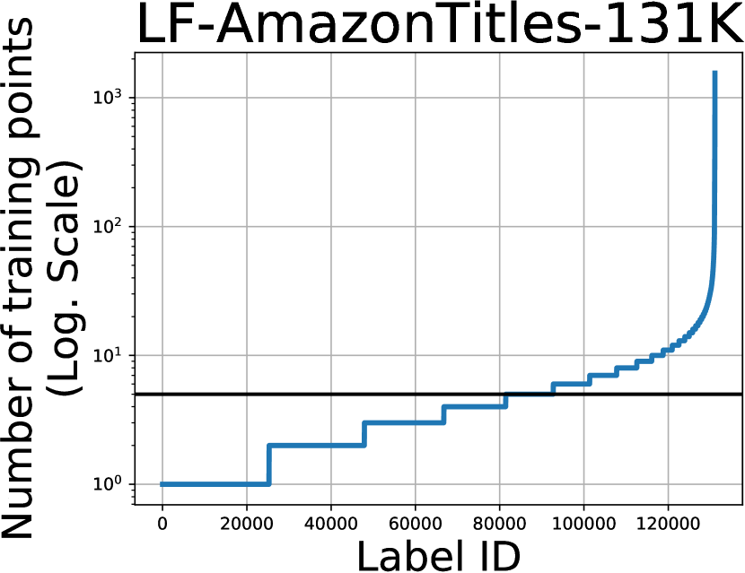
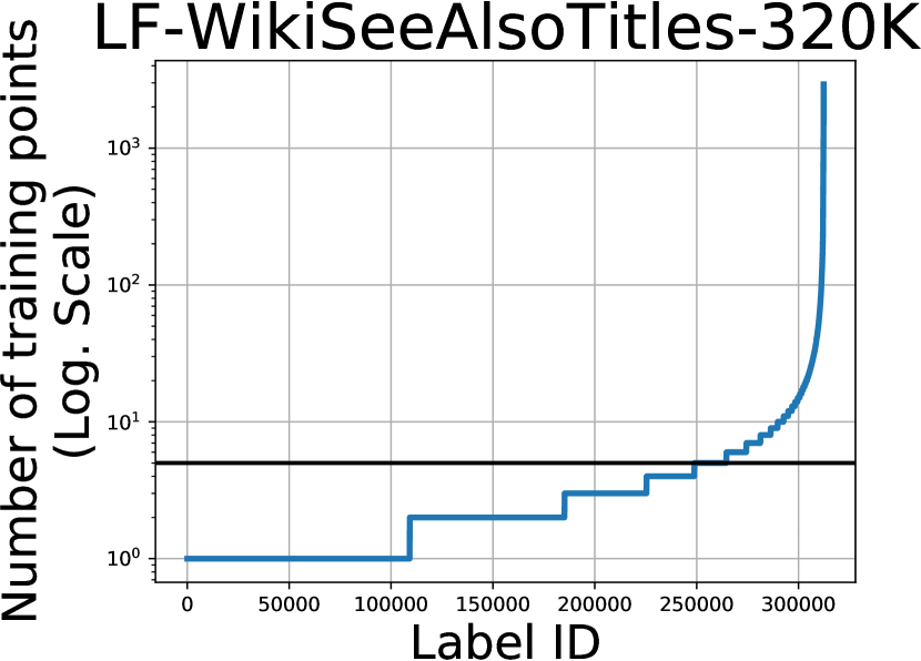
Figure 1. Number of training points per label for two datasets. Labels are ordered from left to right in increasing order of popularity. 60–80% labels have $<5$ training points (the bold horizontal line indicates the 5 training point level).

Rare Labels. XC applications with millions of labels typically find that most labels are rare, with very few training data points tagged with those labels. Fig 1 exemplifies this on two benchmark datasets where 60–80% labels have $<5$ training points. The reasons behind rare labels are manifold. In several XC applications, there may exist an inherent skew in the popularity of labels, e.g, it is natural for certain products to be more popular among users on an e-commerce platform. XC applications also face missing labels (Jain et al., 2016; Yu et al., 2014) where training points are not tagged with all the labels relevant to them. Reasons for this include the inability of human users to exhaustively mark all products of interest to them, and biases in the recommendation platform (e.g. website, app) itself which may present or impress upon its users, certain products more often than others.

Need for Label Metadata. Rare labels are of critical importance in XC applications. They allow highly personalized yet relevant recommendations that may delight and surprise a user, or else allow precise and descriptive tags to be assigned to a document, etc. However, the paucity of training data for rare labels makes it challenging to predict them accurately. Incorporating label metadata such as textual label descriptions (Mittal et al., 2021), label taxonomies (Kanagal et al., 2012; Menon et al., 2011; Sachdeva et al., 2018) and label co-occurrence into the classification process are possible ways to augment the available information for rare labels.

Key Contributions of ECLARE. This paper presents ECLARE, an XC method that performs collaborative learning that benefits rare labels. This is done by incorporating multiple forms of label metadata such as label text as well as dynamically inferred label correlation graphs. Critical to ECLARE are augmentations to the architecture and learning pipeline that scale to millions of labels:

1. Introduce a framework that allows collaborative extreme learning using label-label correlation graphs that are dynamically generated using asymmetric random walks. This is in contrast to existing approaches that often perform collaborative learning on static user-user or document-document graphs (He et al., 2020; Hamilton et al., 2017; Ying et al., 2018).

2. Introduce the use of multiple representations for each label: one learnt from label text alone (LTE), one learnt collaboratively from label correlation graphs (GALE), and a label-specific refinement vector. ECLARE proposes a robust yet inexpensive attention mechanism to fuse these multiple representations to generate a single one-vs-all classifier per label.

3. Propose critical augmentations to well-established XC training steps, such as label clustering, negative sampling, classifier initialization, shortlist creation (GAME), etc, in order to incorporate label correlations in a systematic and scalable manner.

4. Offer an end-to-end training pipeline incorporating the above components in an efficient manner which can be scaled to tasks with millions of labels and offer up to 14% performance boost on standard XC prediction metrics.

Comparison to State-of-the-art. Experiments indicate that apart from significant boosts on standard XC metrics (see Tab 2), ECLARE offers two distinct advantages over existing XC algorithms, including those that do use label metadata such as label text (see Tab 6)

1. Superior Rare Label Prediction: In the first example in Tab 6, for the document “Tibetan Terrier”, ECLARE correctly predicts the rare label “Dog of Osu” that appeared just twice in the training set. All other methods failed to predict this rare label. It is notable that this label has no common tokens (words) with the document text or other labels which indicates that relying solely on label text is insufficient. ECLARE offers far superior performance on propensity scored XC metrics which place more emphasis on predicting rare labels correctly (see Tabs 2 and 3).

2. Superior Intent Disambiguation: The second and third examples in Tab 6 further illustrate pitfalls of relying on label text alone as metadata. For the document “85th Academy Awards”, all other methods are incapable of predicting other award ceremonies held in the same year and make poor predictions. On the other hand, ECLARE was better than other methods at picking up subtle cues and associations present in the training data to correctly identify associated articles. ECLARE offers higher precision@1 and recall@10 (see Tabs 2 and 3).

2. Related Work

Summary. XC algorithms proposed in literature employ a variety of label prediction approaches like tree, embedding, hashing and one-vs-all-based approaches (Babbar and Schölkopf, 2017; Prabhu and Varma, 2014; Prabhu et al., 2018a, b; Jain et al., 2016, 2017; Jain et al., 2019; Babbar and Schölkopf, 2019; Yen et al., 2016, 2017; Yen et al., 2018; Khandagale et al., 2019; Jasinska et al., 2016; Siblini et al., 2018; Jalan and Kar, 2019; Tagami, 2017; Liu et al., 2017; You et al., 2018; Chang et al., 2020; Wydmuch et al., 2018; Guo et al., 2019; Bhatia et al., 2015; Gupta et al., 2019; Dahiya et al., 2021; Mittal et al., 2021). Earlier works learnt label classifiers using fixed representations for documents (typically bag-of-words) whereas contemporary approaches learn a document embedding architecture (typically using deep networks) jointly with the label classifiers. In order to operate with millions of labels, XC methods frequently have to rely on sub-linear time data structures for operations such as shortlisting labels, sampling hard negatives, etc. Choices include hashing (Medini et al., 2019), clustering (Prabhu et al., 2018b; You et al., 2018; Chang et al., 2020), negative sampling (Mikolov et al., 2013), etc. Notably, most XC methods except DECAF (Mittal et al., 2021), GLaS (Guo et al., 2019), and X-Transformer (Chang et al., 2020) do not incorporate any form of label metadata, instead treating labels as black-box identifiers.

Fixed Representation. Much of the early work in XC used fixed bag-of-words (BoW) features to represent documents. One-vs-all methods such as DiSMEC (Babbar and Schölkopf, 2017), PPDSparse (Yen et al., 2017), ProXML (Babbar and Schölkopf, 2019) decompose the XC problem into several binary classification problems, one per label. Although these offered state-of-the-art performance until recently, they could not scale beyond a few million labels. To address this, several approaches were suggested to speed up training (Khandagale et al., 2019; Jain et al., 2019; Prabhu et al., 2018b; Yen et al., 2018), and prediction (Jasinska et al., 2016; Niculescu-Mizil and Abbasnejad, 2017) using tree-based classifiers and negative sampling. These offered high performance as well as could scale to several millions of labels. However, these architectures were suited for fixed features and did not support jointly learning document representations. Attempts, such as (Jain et al., 2019), to use pre-trained features such as FastText (Joulin et al., 2017) were also not very successful if the features were trained on an entirely unrelated task.

Representation Learning. Recent works such as X-Transformer (Chang et al., 2020), ASTEC (Dahiya et al., 2021), XML-CNN (Liu et al., 2017), DECAF (Mittal et al., 2021) and AttentionXML (You et al., 2018) propose architectures that jointly learn representations for the documents as well as label classifiers. For the most part, these methods outperform their counterparts that operate on fixed document representations which illustrates the superiority of task-specific document representations over generic pre-trained features. However, some of these methods utilize involved architectures such as attention (You et al., 2018; Chang et al., 2020) or convolutions (Liu et al., 2017). It has been observed (Dahiya et al., 2021; Mittal et al., 2021) that in addition to being more expensive to train, these architectures also suffer on XC tasks where the documents are short texts, such as user queries, or product titles.

XC with Label Metadata. Utilizing label metadata such as label text, label correlations, etc. can be critical for accurate prediction of rare labels, especially on short-text applications where documents have textual descriptions containing only 5-10 tokens which are not very descriptive. Among existing works, GLaS (Guo et al., 2019) uses label correlations to design a regularizer that improved performance over rare labels, while X-Transformer (Chang et al., 2020) and DECAF (Mittal et al., 2021) use label text as label metadata instead. X-Transformer utilizes label text to perform semantic label indexing (essentially a shortlisting step) along with a pre-trained-then-fine-tuned RoBERTa (Liu et al., 2019) architecture. On the other hand, DECAF uses a simpler architecture to learn both label and document representations in an end-to-end manner.

Collaborative Learning for XC. Given the paucity of data for rare labels, the use of label text alone can be insufficient to ensure accurate prediction, especially in short-text applications such as related products and related queries search, where the amount of label text is also quite limited. This suggests using label correlations to perform collaborative learning on the label side. User-user or document-document graphs (Ying et al., 2018; He et al., 2020; Kipf and Welling, 2017; Tang et al., 2020; Zhang et al., 2020; Hamilton et al., 2017; Velićković et al., 2018; Pal et al., 2020) have become popular, with numerous methods such as GCN (Kipf and Welling, 2017), LightGCN (He et al., 2020), GraphSAGE (Hamilton et al., 2017), PinSage (Ying et al., 2018), etc. utilizing graph neural networks to augment user/document representations. However, XC techniques that directly enable label collaboration with millions of labels have not been explored. One of the major barriers for this seems to be that label correlation graphs in XC applications turn out to be extremely sparse, e.g, for the label correlation graph ECLARE constructed for the LF-WikiSeeAlsoTitles-320K dataset, nearly 18% of labels had no edges to any other label. This precludes the use of techniques such as Personalised Page Rank (PPR) (Ying et al., 2018; Klicpera et al., 2018) over the ground-truth to generate a set of shortlisted labels for negative sampling. ECLARE solves this problem by first mining hard-negatives for each label using a separate technique, and subsequently augmenting this list by adding highly correlated labels.

3. ECLARE: Extreme Classification with Label Graph Correlations

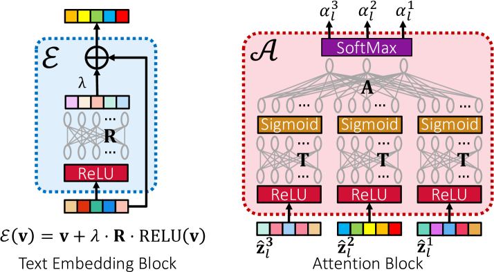
Figure 2. The building blocks of ECLARE. (Left) The embedding block is used in document and label embeddings. (Right) The attention block is used to fuse multiple label representations into a single label classifier (see Fig 3).

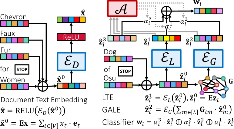
Figure 3. (Left) Document Embedding: ECLARE uses the light-weight embedding block ${\mathcal{E}}$ (see Fig 2) to embed documents, ensuring rapid processing at test time (see Fig 6). Stop words such as for, of) are discarded. (Right) Label classifiers: ECLARE incorporates multiple forms of label metadata including label text (LTE) and label correlation graphs (GALE), fusing them with a per-label refinement vector $\hat{{\mathbf{z}}}^{3}_{l}$ using the attention block (see Fig 2) to create a one-vs-all classifier ${{\mathbf{w}}}_{l}$ for each label $l\in[L]$. Connections to and from the attention block are shown in light gray to avoid clutter. A separate instance of the embedding block is used to obtain document embeddings (${\mathcal{E}}_{D}$), LTE (${\mathcal{E}}_{L}$) and GALE (${\mathcal{E}}_{G}$) embeddings.

Summary. ECLARE consists of four components 1) a text embedding architecture adapted to short-text applications, 2) one-vs-all classifiers, one per label that incorporate label text as well as label correlations, 3) a shortlister that offers high-recall label shortlists for data points, allowing ECLARE to offer sub-millisecond prediction times even with millions of labels, and 4) a label correlation graph that is used to train both the one-vs-all classifiers as well as the shortlister. This section details these components as well as a technique to infer label correlation graphs from training data itself.

Notation. Let $L$ denote the number of labels and $V$ the dictionary size. All $N$ training points are presented as $({{\mathbf{x}}}_{i},{{\mathbf{y}}}_{i})$. ${{\mathbf{x}}}_{i}\in{\mathbb{R}}^{V}$ is a bag-of-tokens representation for the $i\text{${}^{\text{th}}$}$ document i.e. $x_{it}$ is the TF-IDF weight of token $t\in[V]$ in the $i\text{${}^{\text{th}}$}$ document. ${{\mathbf{y}}}_{i}\in\left\{{-1,+1}\right\}^{L}$ is the ground truth label vector with $y_{il}=+1$ if label $l\in[L]$ is relevant to the $i\text{${}^{\text{th}}$}$ document and $y_{il}=-1$ otherwise. For each label $l\in[L]$, its label text is similarly represented as ${{\mathbf{z}}}_{l}\in{\mathbb{R}}^{V}$.

3.1. Document Embedding Architecture

ECLARE learns $D$-dimensional embeddings for each vocabulary token ${{\mathbf{E}}}=\left[{{{\mathbf{e}}}_{1},\ldots,{{\mathbf{e}}}_{V}}\right]\in{\mathbb{R}}^{D\times V}$ and uses a light-weight embedding block (see Fig 2) implementing a residual layer. The embedding block ${\mathcal{E}}$ contains two trainable parameters, a weight matrix ${{\mathbf{R}}}$ and a scalar weight $\lambda$ (see Fig 2). Given a document ${{\mathbf{x}}}\in{\mathbb{R}}^{V}$ as a sparse bag-of-words vector, ECLARE performs a rapid embedding (see Fig 3) by first using the token embeddings to obtain an initial representation $\hat{{\mathbf{x}}}^{0}={{\mathbf{E}}}{{\mathbf{x}}}\in{\mathbb{R}}^{D}$, and then passing this through an instantiation ${\mathcal{E}}_{D}$ of the text embedding block, and a ReLU non-linearity, to obtain the final representation $\hat{{\mathbf{x}}}$. All documents (train/test) share the same embedding block ${\mathcal{E}}_{D}$. Similar architectures have been shown to be well-suited to short-text applications (Dahiya et al., 2021; Mittal et al., 2021).

3.2. Label Correlation Graph

XC applications often fail to provide label correlation graphs directly as an input. Moreover, since these applications also face extreme label sparsity, using label co-occurrence alone yields fractured correlations as discussed in Sec 2. For example, label correlations gleaned from products purchased together in the same session, or else queries on which advertisers bid together, may be very sparse. To remedy this, ECLARE infers a label correlation graph using the ground-truth label vectors i.e. ${{\mathbf{y}}}_{i},i\in[N]$ themselves. This ensures that ECLARE is able to operate even in situations where the application is unable to provide a correlation graph itself. ECLARE adopts a scalable strategy based on random walks with restarts (see Algorithm 1) to obtain a label correlation graph ${{\mathbf{G}}}^{c}\in{\mathbb{R}}^{L\times L}$ that augments the often meager label co-occurrence links (see Fig 4) present in the ground truth. Non-rare labels (the so-called head and torso labels) pose a challenge to this step since they are often correlated with several labels and can overwhelm the rare labels. ECLARE takes two precautions to avoid this:

1. Partition: Head labels (those with $>500$ training points) are disconnected from the graph by setting ${{\mathbf{G}}}^{c}_{hh}=1$ and ${{\mathbf{G}}}^{c}_{ht}=0={{\mathbf{G}}}^{c}_{th}$ for all all head labels $h\in[L]$ and $t\neq h$ (see Fig 5).

2. Normalization: ${{\mathbf{G}}}^{c}$ is normalized to favor edges to/from rare labels as ${{\mathbf{G}}}={{\mathbf{A}}}^{-1/2}\cdot{{\mathbf{G}}}^{c}\cdot{{\mathbf{B}}}^{-1/2}$, where ${{\mathbf{A}}},{{\mathbf{B}}}\in{\mathbb{R}}^{L\times L}$ are diagonal matrices with the row and column-sums of ${{\mathbf{G}}}^{c}$ respectively.

Algorithm 1 is used with a restart probability of 80% and a random walk length of 400. Thus, it is overwhelmingly likely that several dozens of restarts would occur for each label. A high restart probability does not let the random walk wander too far thus preventing tenuous correlations among labels from getting captured.

Algorithm 1 Label Correlation Graph Genration. $N,L$ denote the number of training points and labels. $\omega$ and $p$ denote the walk length and restart probability. ${{\mathbf{Y}}}=[{{\mathbf{y}}}_{1},\ldots,{{\mathbf{y}}}_{N}]\in\left\{{-1,+1}\right\}^{L\times N}$ is a matrix giving the relevant training labels for each document. For any set $S$, $\textrm{Unif}(S)$ returns a uniformly random sample from $S$. The subroutine WalkFrom performs a walk starting at the label $l$.

1:procedure WalkFrom($l,{{\mathbf{Y}}},\omega,p$)

2:     ${{\mathbf{v}}}\leftarrow{\mathbf{0}}\in{\mathbb{R}}^{L}$ $\triangleright$ Initialize visit counts

3:     $\lambda\leftarrow l$ $\triangleright$ Start the walk from the label $l$

4:     for $t=1;t\leq\omega;t$++ do

5:         $\phi\leftarrow\textrm{Unif}([0,1])$  $\triangleright$ Random number in range $[0,1]$

6:         if $\phi\leq p$ then

7:              $\lambda=l$  $\triangleright$ Restart if required          

8:         $\delta\leftarrow\textrm{Unif}(\left\{{i:Y_{\lambda i}=+1}\right\})$  $\triangleright$ Sample a relevant doc

9:         $\lambda\leftarrow\textrm{Unif}(\left\{{j:Y_{j\delta}=+1}\right\})$  $\triangleright$ Sample a relevant label

10:         ${{\mathbf{v}}}[\lambda]$++  $\triangleright$ Update the visit counts      

11:     return ${{\mathbf{v}}}$

12:procedure RandomWalk($L,{{\mathbf{Y}}},\omega,p$)

13:     ${{\mathbf{G}}}^{c}\leftarrow{\mathbf{0}}{\mathbf{0}}^{\top}\in{\mathbb{R}}^{L\times L}$  $\triangleright$ Initialize visit counts

14:     for $l=1;l\leq L;l$++ do

15:         ${{\mathbf{G}}}_{l}^{c}\leftarrow\text{{WalkFrom}}(l,{{\mathbf{Y}}},\omega,p)$  $\triangleright$ Update row $l$ of ${{\mathbf{G}}}^{c}$      

16:     return ${{\mathbf{G}}}^{c}$ 

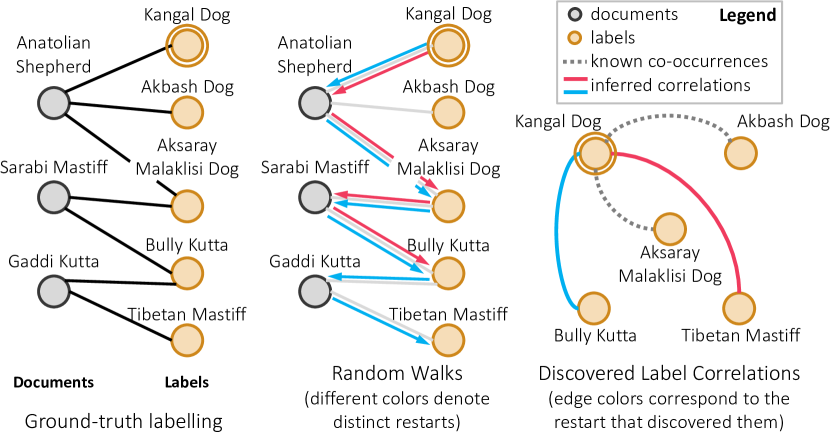
Figure 4. An execution of Algorithm 1 on a subset of the LF-WikiSeeAlsoTitles-320K dataset starting from the label “Kangal Dog”. (Left) ECLARE uses document-label associations taken from ground-truth label vectors (black color) to infer indirect correlations among labels. (Middle) Random walks (distinct restarts colored differently) infer diverse correlations. (Right) These inferred correlations (marked with the color of the restart that discovered them) augment the meager label co-occurrences present in the ground truth (marked with dotted lines).

3.3. Label Representation and Classifiers

As examples in Tab 6 discussed in Sec 4 show, label text alone may not sufficiently inform classifiers for rare labels. ECLARE remedies this by learning high-capacity one-vs-all classifiers ${{\mathbf{W}}}=\left[{{{\mathbf{w}}}_{1},\ldots,{{\mathbf{w}}}_{L}}\right]\in{\mathbb{R}}^{D\times L}$ with 3 distinct components described below.

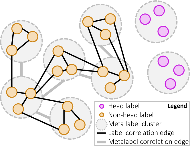
Figure 5. To avoid head labels from distorting label correlation patterns, labels with $>500$ training points are forcibly disconnected from the label correlation graph and also clustered into head meta-labels separately. Consequently, the GALE and GAME steps have a trivial action on head labels.

Label Text Embedding (LTE). The first component incorporates label text metadata. A separate instance ${\mathcal{E}}_{L}$ of the embedding block is used to embed label text. Given a bag-of-words representation ${{\mathbf{z}}}_{l}\in{\mathbb{R}}^{V}$ of a label, the LTE representation is obtained as $\hat{{\mathbf{z}}}^{1}_{l}={\mathcal{E}}_{L}(\hat{{\mathbf{z}}}^{0}_{l})$ where as before, we have the “initial” representation $\hat{{\mathbf{z}}}^{0}_{l}={{\mathbf{E}}}{{\mathbf{z}}}_{l}$. The embedding block ${\mathcal{E}}_{L}$ is shared by all labels. We note that the DECAF method (Mittal et al., 2021) also uses a similar architecture to embed label text.

Graph Augmented Label Embedding (GALE). ECLARE augments the LTE representation using the label correlation graph ${{\mathbf{G}}}$ constructed earlier and a graph convolution network (GCN) (Kipf and Welling, 2017). This presents a departure from previous XC approaches. A typical graph convolution operation consists of two steps which ECLARE effectively implements at extreme scales as shown below

1. Convolution: initial label representations are convolved in a scalable manner using ${{\mathbf{G}}}$ as $\tilde{{\mathbf{z}}}^{2}_{l}=\sum_{m\in[L]}G_{lm}\cdot\hat{{\mathbf{z}}}^{0}_{m}$. Note that due to random restarts used by Algorithm 1, we have $G_{ll}>0$ for all $l\in[L]$ and thus $\tilde{{\mathbf{z}}}^{2}_{l}$ contains a component from $\hat{{\mathbf{z}}}^{0}_{l}$ itself.

2. Transformation: Whereas traditional GCNs often use a simple non-linearity as the transformation, ECLARE instead uses a separate instance ${\mathcal{E}}_{G}$ of the embedding block to obtain the GALE representation of the label as $\hat{{\mathbf{z}}}^{2}_{l}={\mathcal{E}}_{G}(\tilde{{\mathbf{z}}}^{2}_{l})$.

ECLARE uses a single convolution and transformation operation which allowed it to scale to applications with millions of nodes. Recent works such as LightGCN (He et al., 2020) propose to accelerate GCNs by removing all non-linearities. Despite being scalable, using LightGCN itself was found to offer imprecise results in experiments. This may be because ECLARE also uses LTE representations. ECLARE can be seen as improving upon existing GCN architectures such as LightGCN by performing higher order label-text augmentations for $\kappa=0,\ldots,k$ as $\hat{{\mathbf{z}}}^{\kappa+1}_{l}={\mathcal{E}}^{\kappa}_{G}(\sum_{m\in[L]}G^{\kappa}_{lm}\cdot\hat{{\mathbf{z}}}^{0}_{m})$ where ${{\mathbf{G}}}^{\kappa}=\prod_{j=1}^{\kappa}{{\mathbf{G}}}$ encodes the $\kappa-$hop neighborhood, and ${\mathcal{E}}^{\kappa}_{G}$ is a separate embedding block for each order $\kappa$. Thus, ECLARE’s architecture allows parallelizing high-order convolutions. Whereas ECLARE could be used with larger orders $k>1$, using $k=1$ was found to already outperform all competing methods, as well be scalable.

Refinement Vector and Final Classifier. ECLARE combines the LTE and GALE representations for a label with a high-capacity per-label refinement vector $\hat{{\mathbf{z}}}^{3}_{l}\in{\mathbb{R}}^{D}$ (for a general value of $k$, $\hat{{\mathbf{z}}}^{k+2}_{l}$ is used) to obtain a one-vs-all classifier ${{\mathbf{w}}}_{l}$ (see Fig 3). To combine $\hat{{\mathbf{z}}}^{1}_{l},\hat{{\mathbf{z}}}^{2}_{l},\hat{{\mathbf{z}}}^{3}_{l}$, ECLARE uses a parameterized attention block ${\mathcal{A}}$ (see Fig 2) to learn label-specific attention weights for the three components. This is distinct from previous works such as DECAF which use weights that are shared across labels. Fig 9 shows that ECLARE benefits from this flexibility, with the refinement vector $\hat{{\mathbf{z}}}^{3}_{l}$ being more dominant for popular labels that have lots of training data whereas the label metadata based vectors $\hat{{\mathbf{z}}}^{2}_{l},\hat{{\mathbf{z}}}^{1}_{l}$ being more important for rare labels with less training data. The attention block is explained below (see also Fig 2). Recall that ECLARE uses $k=1$.

$$t({{\mathbf{x}}}) =\sigma({{\mathbf{T}}}\cdot\text{ReLU}({{\mathbf{x}}}))$$

$${{\mathbf{q}}}_{l} =\left[{t(\hat{{\mathbf{z}}}^{1}_{l});\ldots;t(\hat{{\mathbf{z}}}^{k+2}_{l})}\right]$$

$$\left[{\alpha^{1}_{l},\ldots,\alpha^{k+2}_{l}}\right] =\frac{\exp({{\mathbf{A}}}\cdot{{\mathbf{q}}}_{l})}{\left\lVert{\exp({{\mathbf{A}}}\cdot{{\mathbf{q}}}_{l})}\right\rVert_{1}}$$

$${{\mathbf{w}}}_{l} =\alpha^{1}_{l}\cdot\hat{{\mathbf{z}}}^{1}_{l}+\ldots+\alpha^{k+2}_{l}\cdot\hat{{\mathbf{z}}}^{k+2}_{l}$$

The attention block is parameterized by the matrices ${{\mathbf{T}}}\in{\mathbb{R}}^{D\times D}$ and ${{\mathbf{A}}}\in{\mathbb{R}}^{(k+2)\times(k+2)D}$. ${{\mathbf{q}}}_{l}\in{\mathbb{R}}^{(k+2)D}$ concatenates the transformed components before applying the attention layer ${{\mathbf{A}}}$. The above attention mechanism can be seen as a scalable paramaterized option (requiring only ${\mathcal{O}}\left({{D^{2}+k^{2}D}}\right)$ additional parameters) instead of a more expensive label-specific attention scheme which would have required learning $L\times(k+2)$ parameters.

3.4. Meta-labels and the Shortlister

Despite being accurate, if used naively, one-vs-all classifiers require $\Omega\left({{LD}}\right)$ time at prediction and $\Omega\left({{NLD}}\right)$ time to train. This is infeasible with millions of labels. As discussed in Sec 2, sub-linear structures are a common remedy in XC methods to perform label shortlisting during prediction (Khandagale et al., 2019; Prabhu et al., 2018b; Yen et al., 2017; Chang et al., 2020; Jain et al., 2019; Bhatia et al., 2015; Dahiya et al., 2021). These shortlisting techniques take a data point and return a shortlist of ${\mathcal{O}}\left({{\log L}}\right)$ labels that is expected to contain most of the positive labels for that data point. However, such shortlists also help during training since the negative labels that get shortlisted for a data point are arguably the most challenging and likely to get confused as being positive for that data point. Thus, one-vs-all classifiers are trained only on positive and shortlisted negative labels, bringing training time down to ${\mathcal{O}}\left({{ND\log L}}\right)$. Similar to previous works (Prabhu et al., 2018a; Mittal et al., 2021), ECLARE uses a clustering-based shortlister ${\mathcal{S}}=\left\{{{\mathcal{C}},{{\mathbf{H}}}}\right\}$ where ${\mathcal{C}}=\left\{{C_{1},\ldots,C_{{K}}}\right\}$ is a balanced partitioning of the $L$ labels into $K$ clusters. We refer to each cluster as a meta label. ${{\mathbf{H}}}=[{{\mathbf{h}}}_{1},\ldots,{{\mathbf{h}}}_{K}]\in{\mathbb{R}}^{D\times K}$ is a set of one-vs-all classifiers, learnt one per meta label.

Graph Assisted Multi-label Expansion (GAME). ECLARE incorporates graph correlations to further to improve its shortlister. Let ${{\mathbf{M}}}\in\left\{{0,1}\right\}^{L\times K}$ denote the cluster assignment matrix i.e. $M_{lm}=1$ if label $l$ is in cluster $m$. We normalize ${{\mathbf{M}}}$ so that each column sums to unity. Given a data point ${{\mathbf{x}}}$ and a beam-size $B$, its embedding $\hat{{\mathbf{x}}}$ (see Fig 3) is used to shortlist labels as follows

1. Find the top $B$ clusters, say $P=\left\{{\tilde{m}_{1},\ldots,\tilde{m}_{B}}\right\}\subset[K]$ according to the meta-label scores $\left\langle{{{\mathbf{h}}}_{m_{1}}},{\hat{{\mathbf{x}}}}\right\rangle\geq\left\langle{{{\mathbf{h}}}_{m_{2}}},{\hat{{\mathbf{x}}}}\right\rangle\geq\ldots$. Let $\tilde{{\mathbf{p}}}\in{\mathbb{R}}^{K}$ be a vector containing scores for the top $B$ clusters passed through a sigmoid i.e. $\tilde{p}_{m}=\sigma(\left\langle{{{\mathbf{h}}}_{m}},{\hat{{\mathbf{x}}}}\right\rangle)$ if $m\in P$ else $\tilde{p}_{m}=0$.

2. Use the induced cluster-cluster correlation matrix ${{\mathbf{G}}}_{M}={{\mathbf{M}}}^{\top}{{\mathbf{G}}}{{\mathbf{M}}}$ to calculate the “GAME-ified” scores ${{\mathbf{p}}}={{\mathbf{G}}}_{M}\cdot\tilde{{\mathbf{p}}}$.

3. Find the top $B$ clusters according to ${{\mathbf{p}}}$, say $m_{1},\ldots,m_{B}$, retain their scores and set scores of other clusters in ${{\mathbf{p}}}$ to $0$. Return the shortlist ${\mathcal{S}}(\hat{{\mathbf{x}}})=\left\{{m_{1},\ldots,m_{B}}\right\}$ and the modified score vector ${{\mathbf{p}}}$.

Note that this cluster re-ranking step uses an induced cluster correlation graph and can bring in clusters with rare labels missed by the one-vs-all models ${{\mathbf{h}}}_{m}$. This is distinct from previous works which do not use label correlations for re-ranking. Since the clusters are balanced, the shortlisted clusters always contain a total of $|{\mathcal{S}}(\hat{{\mathbf{x}}})|=LB/K$ labels. ECLARE uses $K=2^{17}$ clusters and a beam size of $B\approx 30-50$ (see Sec 4 for a discussion on hyperparameters).

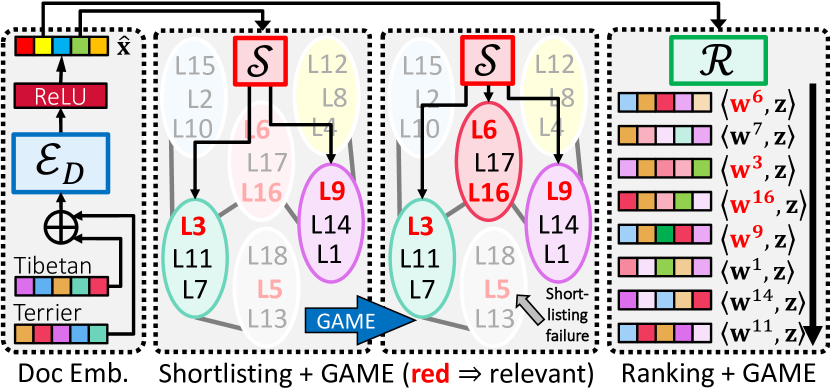
Figure 6. Prediction Pipeline: ECLARE uses a low-cost prediction pipeline that can make millisecond-level predictions with millions of labels. Given a document/query ${{\mathbf{x}}}$, its text embedding $\hat{{\mathbf{x}}}$ (see Fig 3) is used by the shortlister ${\mathcal{S}}$ to obtain the ${\mathcal{O}}\left({{\log L}}\right)$ most probable labels while maintaining high recall using label correlation graphs via GAME. Label classifiers (see Fig 3) for only the shortlisted labels are then used by the ranker ${\mathcal{R}}$ to produce the final ranking of labels.

3.5. Prediction with GAME

The prediction pipeline for ECLARE is depicted in Fig 6 and involves 3 steps that repeatedly utilize label correlations via GAME.

1. Given a document ${{\mathbf{x}}}$, use the shortlister ${\mathcal{S}}$ to get a set of $B$ meta labels ${\mathcal{S}}(\hat{{\mathbf{x}}})$ and their corresponding scores ${{\mathbf{p}}}\in{\mathbb{R}}^{K}$.

2. For shortlisted labels, apply the one-vs-all classifiers ${{\mathbf{w}}}_{l}$ to calculate the ranking score vector $\tilde{{\mathbf{r}}}\in{\mathbb{R}}^{L}$ with $\tilde{r}_{l}=\sigma(\left\langle{{{\mathbf{w}}}_{l}},{\hat{{\mathbf{x}}}}\right\rangle)$ if $l\in C_{m}$ for some $m\in{\mathcal{S}}(\hat{{\mathbf{x}}})$ else $\tilde{r}_{l}=0$.

3. GAME-ify the one-vs-all scores to get ${{\mathbf{r}}}={{\mathbf{G}}}\cdot\tilde{{\mathbf{r}}}$ (note that ${{\mathbf{G}}}$ is used this time and not ${{\mathbf{G}}}_{M}$). Make final predictions using the joint scores $s_{l}:=r_{l}\cdot p_{m}$ if $l\in C_{m},m\in{\mathcal{S}}(\hat{{\mathbf{x}}})$ else $s_{l}=0$.

3.6. Efficient Training: the DeepXML Pipeline

Summary. ECLARE adopts the scalable DeepXML pipeline (Dahiya et al., 2021) that splits training into 4 modules. In summary, Module I jointly learns the token embeddings ${{\mathbf{E}}}$, the embedding block ${\mathcal{E}}_{D}$ and the shortlister ${\mathcal{S}}$. ${{\mathbf{E}}}$ remains frozen hereon. Module II refines ${\mathcal{P}}$ and uses it to retrieve label shortlists for all data points. After performing initialization in Module III, Module IV uses the shortlists generated in Module II to jointly fine-tune ${\mathcal{E}}_{D}$ and learn the one-vs-all classifiers ${{\mathbf{W}}}$, implicitly learning the embedding blocks ${\mathcal{E}}_{L},{\mathcal{E}}_{G}$ and the attention block ${\mathcal{A}}$ in the process.

Module I. Token embeddings ${{\mathbf{E}}}\in{\mathbb{R}}^{D\times V}$ are randomly initialized using (He et al., 2015), the residual block within ${\mathcal{E}}_{D}$ is initialized to identity. After creating label clusters (see below), each cluster is treated as a meta-label yielding a meta-XC problem on the same training points, but with $K$ meta-labels instead of the original $L$ labels. Meta-label text is created for each $m\in[K]$ as ${{\mathbf{u}}}_{m}=\sum_{l\in C_{m}}{{\mathbf{z}}}_{l}$. Meta labels are also endowed with the meta-label correlation graph ${{\mathbf{G}}}_{M}={{\mathbf{M}}}^{\top}{{\mathbf{G}}}{{\mathbf{M}}}$ where ${{\mathbf{M}}}\in\left\{{0,1}\right\}^{L\times K}$ is the cluster assignment matrix. One-vs-all meta-classifiers ${{\mathbf{H}}}=[{{\mathbf{h}}}_{1},\ldots,{{\mathbf{h}}}_{K}]\in{\mathbb{R}}^{D\times K}$ are now learnt to solve this meta XC problem. These classifiers have the same form as those for the original problem with 3 components, LTE, GALE, (with corresponding blocks $\tilde{\mathcal{E}}_{L},\tilde{\mathcal{E}}_{G}$) and refinement vector, with an attention block $\tilde{\mathcal{A}}$ supervising their combination (parameters within $\tilde{\mathcal{A}}$ are initialized randomly). However, in Module-I, refinement vectors are turned off for ${{\mathbf{h}}}_{l}$ to force good token embeddings ${{\mathbf{E}}}$ to be learnt without support from refinement vectors. Module I solves the meta XC problem while training ${\mathcal{E}}_{D},\tilde{\mathcal{E}}_{L},\tilde{\mathcal{E}}_{G},\tilde{\mathcal{A}},{{\mathbf{E}}}$, implicitly learning ${{\mathbf{H}}}$.

Meta-label Creation with Graph Augmented Label Centroids. Existing approaches such as Parabel or DECAF cluster labels by creating a label centroid for each label $l$ by aggregating features for training documents associated with that label as ${{\mathbf{c}}}_{l}=\sum_{i:y_{il}=+1}{{\mathbf{x}}}_{i}$. However, ECLARE recognizes that missing labels often lead to an incomplete ground truth, and thus, poor label centroids for rare labels in XC settings (Jain et al., 2017; Babbar and Schölkopf, 2019). Fig 8 confirms this suspicion. ECLARE addresses this by augmenting the label centroids using the label co-occurrence graph ${{\mathbf{G}}}$ to redefine the centroids as $\hat{{\mathbf{c}}}_{l}=\sum_{j=1}^{L}G_{lj}\cdot{{\mathbf{c}}}_{l}$. Balanced hierarchical binary clustering (Prabhu et al., 2018b) is now done on these label centroids for 17 levels to generate $K=2^{17}$ label clusters. Note that since token embeddings have not been learnt yet, the raw TF-IDF documents vectors ${{\mathbf{x}}}_{i}\in{\mathbb{R}}^{V}$ are used instead of $\hat{{\mathbf{x}}}_{i}\in{\mathbb{R}}^{D}$.

Module II. The shortlister is fine-tuned in this module. Label centroids are recomputed as $\hat{{\mathbf{c}}}_{l}=\sum_{j=1}^{L}G_{lj}\cdot{{\mathbf{c}}}_{l}$ where this time, ${{\mathbf{c}}}_{l}=\sum_{i:{{\mathbf{y}}}^{i}_{l}=+1}{{\mathbf{E}}}{{\mathbf{x}}}_{i}$ using ${{\mathbf{E}}}$ learnt in Module I. The meta XC problem is recreated and solved again. However, this time, ECLARE allows the meta-classifiers ${{\mathbf{h}}}_{m}$ to also include refinement vectors to better solve the meta-XC problem. In the process of re-learning ${{\mathbf{H}}}$, the model parameters ${\mathcal{E}}_{D},\tilde{\mathcal{E}}_{L},\tilde{\mathcal{E}}_{G},\tilde{\mathcal{A}}$ are fine-tuned (${{\mathbf{E}}}$ is frozen after Module I). The shortlister ${\mathcal{S}}$ thus obtained is thereafter used to retrieve shortlists ${\mathcal{S}}(\hat{{\mathbf{x}}}_{i})$ for each data point $i\in[N]$. However, distinct from previous work such as Slice (Jain et al., 2019), X-Transformer (Chang et al., 2020), DECAF (Mittal et al., 2021), ECLARE uses the GAME strategy to obtain negative samples that take label correlations into account.

Module III. Residual blocks within ${\mathcal{E}}_{D},{\mathcal{E}}_{L},{\mathcal{E}}_{G}$ are initialized to identity, parameters within ${\mathcal{A}}$ are initialized randomly, and the shortlister ${\mathcal{S}}$ and token embeddings ${{\mathbf{E}}}$ are kept frozen. Refinement vectors for all $L$ labels are initialized to $\hat{{\mathbf{z}}}^{3}_{l}=\sum_{m\in[L]}G_{lm}\cdot{{\mathbf{E}}}{{\mathbf{z}}}_{m}$. We find this initialization to be both crucial (see Sec 4) as well as distinct from previous works such as DECAF which initialized its counterpart of refinement vectors using simply ${{\mathbf{E}}}{{\mathbf{z}}}_{l}$. Such correlation-agnostic initialization was found to offer worse results than ECLARE’s graph augmented initialization.

Module IV. In this module, the embedding blocks ${\mathcal{E}}_{D},{\mathcal{E}}_{L},{\mathcal{E}}_{G}$ are learnt jointly with the per-label refinement vectors $\hat{{\mathbf{z}}}^{3}_{l}$ and attention block ${\mathcal{A}}$, thus learning the one-vs-all classifiers ${{\mathbf{w}}}_{l}$ in the process, However, training is done in ${\mathcal{O}}\left({{ND\log L}}\right)$ time by restricting training to positives and shortlisted negatives for each data point.

Loss Function and Regularization. ECLARE uses the binary cross entropy loss function for training in Modules I, II and IV using the Adam (Kingma and Ba, 2014) optimizer. The residual weights ${{\mathbf{R}}}$ in the various embedding blocks ${\mathcal{E}}_{D},{\mathcal{E}}_{L},{\mathcal{E}}_{G},\tilde{\mathcal{E}}_{L},\tilde{\mathcal{E}}_{G}$ as well as the weights ${{\mathbf{T}}}$ in the attention block were all subjected to spectral regularization (Miyato et al., 2018). All ReLU layers in the architecture also included a dropout layer with 20% rate.

Key Contributions in Training. ECLARE markedly departs from existing techniques by incorporating label correlation information in a scalable manner at every step of the learning process. Right from Module I, label correlations are incorporated while creating the label centroids leading to higher quality clusters (see Fig 8 and Table 7). The architecture itself incorporates label correlation information using the GALE representations. It is crucial to initialize the refinement vectors $\hat{{\mathbf{z}}}^{3}_{l}$ properly for which ECLARE uses a graph-augmented initialization. ECLARE continues infusing label correlation during negative sampling using the GAME step. Finally, GAME is used multiple times in the prediction pipeline as well. As the discussion in Sec 4 will indicate, these augmentations are crucial to the performance boosts offered by ECLARE.

4. Experiments

Table 1. Dataset Statistics. A $\ddagger$ sign denotes information that was redacted for proprietary datasets. The first four rows are public datasets and the last two rows are proprietary datasets. Dataset names with an asterisk ^∗ next to them correspond to product-to-category tasks whereas others are product-to-product tasks.

Dataset	Train Documents $N$	Labels $L$	Tokens $V$	Test Instances $N^{\prime}$	Average Labels per Document	Average Points per label	Average Tokens per Document	Average Tokens per Label
Short text dataset statistics
LF-AmazonTitles-131K	294,805	131,073	40,000	134,835	2.29	5.15	7.46	7.15
LF-WikiSeeAlsoTitles-320K	693,082	312,330	40,000	177,515	2.11	4.68	3.97	3.92
LF-WikiTitles-500K∗	1,813,391	501,070	80,000	783,743	4.74	17.15	3.72	4.16
LF-AmazonTitles-1.3M	2,248,619	1,305,265	128,000	970,237	22.20	38.24	9.00	9.45
Proprietary dataset
LF-P2PTitles-2M	2,539,009	1,640,898	$\ddagger$	1,088,146	$\ddagger$	$\ddagger$	$\ddagger$	$\ddagger$
LF-P2PTitles-10M	6,849,451	9,550,772	$\ddagger$	2,935,479	$\ddagger$	$\ddagger$	$\ddagger$	$\ddagger$

Table 2. Results on public benchmark datasets. ECLARE could offer 2-3.5% higher P@1 as well as upto 5% higher PSP@1 which focuses on rare labels. Additionally, ECLARE offered up to 3% better recall than leading XC methods.

Method	PSP@1	PSP@5	P@1	P@5	R@10	Prediction Time (ms)
LF-AmazonTitles-131K
ECLARE	33.51	44.7	40.74	19.88	54.11	0.1
DECAF	30.85	41.42	38.4	18.65	51.2	0.1
Astec	29.22	39.49	37.12	18.24	49.87	2.34
AttentionXML	23.97	32.57	32.25	15.61	42.3	5.19
Slice	23.08	31.89	30.43	14.84	41.16	1.58
MACH	24.97	34.72	33.49	16.45	44.75	0.23
X-Transformer	21.72	27.09	29.95	13.07	35.59	15.38
Siamese	13.3	13.36	13.81	5.81	14.69	0.2
Bonsai	24.75	34.86	34.11	16.63	45.17	7.49
Parabel	23.27	32.14	32.6	15.61	41.63	0.69
DiSMEC	25.86	36.97	35.14	17.24	46.84	5.53
XT	22.37	31.64	31.41	15.48	42.11	9.12
AnneXML	19.23	32.26	30.05	16.02	45.57	0.11
LF-WikiSeeAlsoTitles-320K
ECLARE	22.01	26.27	29.35	15.05	36.46	0.12
DECAF	16.73	21.01	25.14	12.86	32.51	0.09
Astec	13.69	17.5	22.72	11.43	28.18	2.67
AttentionXML	9.45	11.73	17.56	8.52	20.56	7.08
Slice	11.24	15.2	18.55	9.68	24.45	1.85
MACH	9.68	12.53	18.06	8.99	22.69	0.52
Siamese	10.1	9.59	10.69	4.51	10.34	0.17
Bonsai	10.69	13.79	19.31	9.55	23.61	14.82
Parabel	9.24	11.8	17.68	8.59	20.95	0.8
DiSMEC	10.56	14.82	19.12	9.87	24.81	11.02
XT	8.99	11.82	17.04	8.6	21.73	12.86
AnneXML	7.24	11.75	16.3	8.84	23.06	0.13
LF-AmazonTitles-1.3M
ECLARE	23.43	30.56	50.14	40	32.02	0.32
DECAF	22.07	29.3	50.67	40.35	31.29	0.16
Astec	21.47	27.86	48.82	38.44	29.7	2.61
AttentionXML	15.97	22.54	45.04	36.25	26.26	29.53
Slice	13.96	19.14	34.8	27.71	20.21	1.45
MACH	9.32	13.26	35.68	28.35	19.08	2.09
Bonsai	18.48	25.95	47.87	38.34	29.66	39.03
Parabel	16.94	24.13	46.79	37.65	28.43	0.89
DiSMEC	-	-	-	-	-	-
XT	13.67	19.06	40.6	32.01	22.51	5.94
AnneXML	15.42	21.91	47.79	36.91	26.79	0.12
LF-WikiTitles-500K
ECLARE	21.58	19.84	44.36	16.91	30.59	0.14
DECAF	19.29	19.96	44.21	17.36	32.02	0.09
Astec	18.31	18.56	44.4	17.49	31.58	2.7
AttentionXML	14.8	13.88	40.9	15.05	25.8	9
Slice	13.9	13.82	25.48	10.98	22.65	1.76
MACH	13.71	12	37.74	13.26	23.81	0.8
Bonsai	16.58	16.4	40.97	15.66	28.04	17.38
Parabel	15.55	15.35	40.41	15.42	27.34	0.81
DiSMEC	15.88	15.89	39.42	14.85	26.73	11.71
XT	14.1	14.38	38.13	14.66	26.48	7.56
AnneXML	13.91	13.75	39	14.55	26.27	0.13

Table 3. Results on proprietary product-to-product (P2P) recommendation datasets. ECLARE could offer significant gains – upto 14% higher P@1, 15% higher PSP@1 and 7% higher R@10 – than competing classifiers.

Method	PSP@1	PSP@3	PSP@5	P@1	P@3	P@5	R@10
LF-P2PTitles-2M
ECLARE	41.97	44.92	49.46	43.79	39.25	33.15	54.44
DECAF	36.65	40.14	45.15	40.27	36.65	31.45	48.46
Astec	32.75	36.3	41	36.34	33.33	28.74	46.07
Parabel	30.21	33.85	38.46	35.26	32.44	28.06	42.84
LF-P2PTitles-10M
ECLARE	35.52	37.91	39.91	43.14	39.93	36.9	35.82
DECAF	20.51	21.38	22.85	28.3	25.75	23.99	20.9
Astec	20.31	22.16	24.23	29.75	27.49	25.85	22.3
Parabel	19.99	22.05	24.33	30.22	27.77	26.1	22.81

Table 4. An ablation study exploring the benefits of the GAME step for other XC methods. Although ECLARE still provides the leading accuracies, existing methods show consistent gains from the use of the GAME step.

Method	PSP@1	PSP@5	P@1	P@5	PSP@1	PSP@5	P@1	P@5
LF-AmazonTitles-131K
	Original    |				With GAME
ECLARE	-	-	-	-	33.51	44.7	40.74	19.88
Parabel	23.27	32.14	32.6	15.61	24.81	34.94	33.24	16.51
AttentionXML	23.97	32.57	32.25	15.61	24.63	34.48	32.59	16.25
LF-WikiSeeAlsoTitles-320K
	Original    |				With GAME
ECLARE	-	-	-	-	22.01	26.27	29.35	15.05
Parabel	9.24	11.8	17.68	8.59	10.28	13.06	17.99	9
AttentionXML	9.45	11.73	17.56	8.52	10.05	12.59	17.49	8.77

Datasets and Features. ECLARE was evaluated on 4 publicly available benchmark datasets, LF-AmazonTitles-131K, LF-WikiSeeAlso-Titles-320K, LF-WikiTitles-500K and LF-AmazonTitles-1.3M. These datasets were derived from existing datasets e.g. Amazon-670K, by taking those labels for which label text was available and performing other sanitization steps such as reciprocal pair removal (see (Mittal et al., 2021) for details). ECLARE was also evaluated on proprietary datasets P2P-2M and P2P-10M, both mined from click logs of the Bing search engine, where a pair of products were considered similar if the Jaccard index of the set of queries which led to a click on them was found to be more than a certain threshold. ECLARE used the word piece tokenizer (Schuster and Nakajima, 2012) to create a shared vocabulary for documents and labels. Please refer to Tab 1 for dataset statistics.

Baseline algorithms. ECLARE’s performance was compared to state-of-the-art deep extreme classifiers which jointly learn document and label representations such as DECAF (Mittal et al., 2021), AttentionXML (You et al., 2018), Astec (Dahiya et al., 2021), X-Transformer (Chang et al., 2020), and MACH (Medini et al., 2019). DECAF and X-Transformer are the only methods that also use label text and are therefore the most relevant for comparison with ECLARE. For the sake of completeness, ECLARE was also compared to classifiers which use fixed document representations like DiSMEC (Babbar and Schölkopf, 2017), Parabel (Prabhu et al., 2018b), Bonsai (Khandagale et al., 2019), and Slice (Jain et al., 2019). All these fixed-representation methods use BoW features, except Slice which used pre-trained FastText (Bojanowski et al., 2017) features. The GLaS (Guo et al., 2019) method could not be included in our analysis as its code was not publicly available.

Evaluation. Methods were compared using standard XC metrics, namely Precision (P@$k$) and Propensity-scored precision (PSP@$k$) (Jain et al., 2017). Recall (R@$K$) was also included since XC methods are typically used in the shortlisting pipeline of recommendation systems. Thus, having high recall is equally important as having high precision. For evaluation, guidelines provided on the XML repository (Bhatia et al., 2016) were followed. To be consistent, all models were run on a 6-core Intel Skylake 2.4 GHz machine with one Nvidia V100 GPU.

Hyper-parameters. A beam size of $B=30$ was used for the dataset LF-AmazonTitles-131K and $B=50$ for all other datasets. Embedding dimension $D$ was set to 300 for datasets with $<400$K labels and 512 otherwise. The number of meta-labels $K=|{\mathcal{C}}|$ was fixed to $|{\mathcal{C}}|=2^{17}$ for all other datasets except for LF-AmazonTitles-131K where $|{\mathcal{C}}|=2^{15}$ was chosen since the dataset itself has around $2^{17}$ labels. The default PyTorch implementation of the Adam optimizer was used. Dropout with probability 0.2 was used for all datasets. Learning rate was decayed by a decay factor of 0.5 after an interval of $0.5\times$ epoch length. Batch size was taken to be 255 for all datasets. ECLARE Module-I used 20 epochs with an initial learning rate of 0.01. In Modules-II and IV, 10 epochs were used for all datasets with an initial learning rate of 0.008. While constructing the label correlation graph using random walks (see Algorithm 1), a walk length of $400$ and restart probability of $80\%$ were used for all datasets.

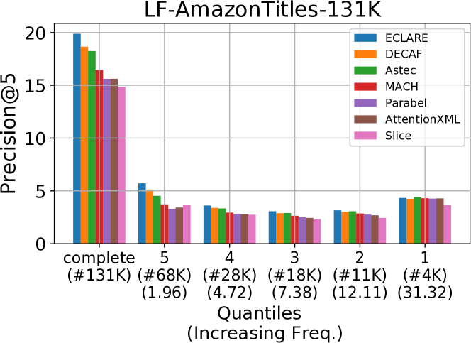
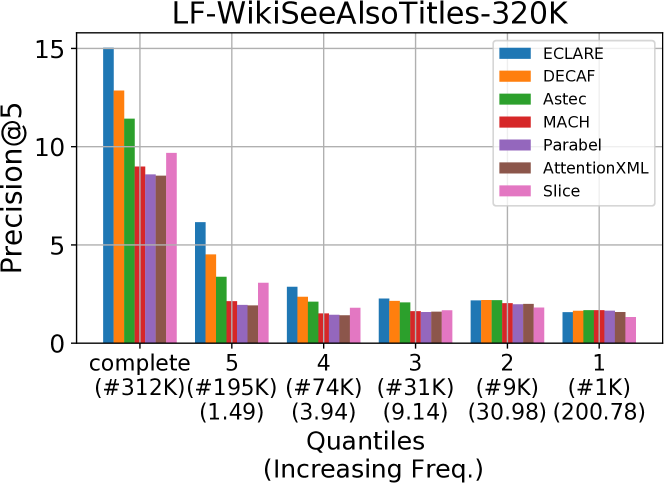
Figure 7. Analyzing the performance of ECLARE and other methods on popular vs rare labels. Labels were divided into 5 bins in increasing order of popularity. The plots show the overall P@5 for each method (histogram group “complete”) and how much each bin contributed to this value. ECLARE clearly draws much of its P@5 performance from the bin with the rarest labels (histogram group 5), i.e ECLARE’s superiority over other methods in terms of P@5 comes from predicting challenging rare labels and not easy-to-predict popular labels. ECLARE’s lead over other methods is also more prominent for rare bins (histogram groups 4, 5).

Results on benchmark datasets. Tab 2 demonstrates that ECLARE can be significantly more accurate than existing XC methods. In particular, ECLARE could be upto 3% and 10% more accurate as compared to DECAF and X-Transformer respectively in terms of P@$1$. It should be noted that DECAF and X-Transformer are the only XC methods which use label meta-data. Furthermore, ECLARE could outperform Astec which is specifically designed for rare labels, by up to 7% in terms of PSP@$1$, indicating that ECLARE offers state-of-the-art accuracies without compromising on rare labels. To further understand the gains of ECLARE, the labels were divided into five bins such that each bin contained an equal number of positive training points (Fig 7). This ensured that each bin had an equal opportunity to contribute to the overall accuracy. Fig 7 indicates that the major gains of ECLARE come from predicting rare labels correctly. ECLARE could outperform all other deep-learning-based XC methods, as well as fixed-feature-based XC methods by a significant margin of at least 7%. Moreover, ECLARE’s recall could be up to 2% higher as compared to all other XC methods.

Results on Propreitary Bing datasets. ECLARE’s performance was also compared on the proprietary datasets LF-P2PTitles-2M and LF-P2PTitles-10M. Note that ECLARE was only compared with those XC methods that were able to scale to 10 million labels on a single GPU within a timeout of one week. ECLARE could be up to 14%, 15%, and 15% more accurate as compared to state-of-the-art methods in terms of P@$1$, PSP@$1$ and R@$10$ respectively. Please refer to Tab 3 for more details.

Table 5. An ablation study exploring alternate design decisions. Design choices made by ECLARE for its components were found to be optimal among popular alternatives.

Method	PSP@1	PSP@3	PSP@5	P@1	P@3	P@5
LF-AmazonTitles-131K
ECLARE	33.51	39.55	44.7	40.74	27.54	19.88
ECLARE-GCN	24.02	29.32	34.02	30.94	21.12	15.52
ECLARE-LightGCN	31.36	36.79	41.58	38.39	25.59	18.44
ECLARE-Cooc	32.82	38.67	43.72	39.95	26.9	19.39
ECLARE-PN	32.49	38.15	43.25	39.63	26.64	19.24
ECLARE-PPR	12.51	16.42	20.25	14.42	11.04	8.75
ECLARE-NoGraph	30.49	36.09	41.13	37.45	25.45	18.46
ECLARE-NoLTE	32.3	37.88	42.87	39.33	26.41	19.05
ECLARE-NoRefine	28.18	33.14	38.3	29.99	21.6	16.32
ECLARE-SUM	31.45	36.73	41.65	38.02	25.54	18.49
ECLARE-k=2	32.23	38.06	43.23	39.38	26.57	19.22
ECLARE-8K	29.98	35.08	39.71	37	24.86	17.93
LF-WikiSeeAlsoTItles-320K
ECLARE	22.01	24.23	26.27	29.35	19.83	15.05
ECLARE-GCN	13.76	15.88	17.67	21.76	14.61	11.14
ECLARE-LightGCN	19.05	21.24	23.14	26.31	17.64	13.35
ECLARE-Cooc	20.96	23.1	25.07	28.54	19.06	14.4
ECLARE-PN	20.42	22.56	24.59	28.24	18.88	14.3
ECLARE-PPR	4.83	5.53	7.12	5.21	3.82	3.5
ECLARE-NoGraph	18.44	20.49	22.42	26.11	17.59	13.35
ECLARE-NoLTE	20.16	22.22	24.16	27.73	18.48	13.99
ECLARE-NoRefine	20.27	21.26	22.8	24.83	16.61	12.66
ECLARE-SUM	20.59	22.48	24.36	27.59	18.5	13.99
ECLARE-k=2	20.12	22.38	24.43	27.77	18.64	14.14
ECLARE-8K	13.42	15.03	16.47	20.31	13.51	10.22

Ablation experiments. To scale accurately to millions of labels, ECLARE makes several meticulous design choices. To validate their importance, Tab 5 compares different variants of ECLARE:

1. Label-graph augmentations: The label correlation graph ${{\mathbf{G}}}$ is used by ECLARE in several steps, such as in creating meaningful meta labels, negative sampling, shortlisting of meta-labels, etc. To evaluate the importance of these augmentations, in ECLARE-NoGraph, the graph convolution component ${{\mathbf{G}}}$ was removed from all training steps such as GAME, except while generating the label classifiers (GALE). ECLARE-NoGraph was found to be up to 3% less accurate than ECLARE. Furthermore, in a variant ECLARE-PPR, inspired by state-of-the-art graph algorithms (Ying et al., 2018; Klicpera et al., 2018), negative sampling was performed via Personalized Page Rank. ECLARE could be up to 25% more accurate than ECLARE-PPR. This could be attributed to the highly sparse label correlation graph and justifies the importance of ECLARE’s label correlation graph as well as it’s careful negative sampling.

2. Label components: Much work has been done to augment (document) text representations using graph convolution networks (GCNs) (Tang et al., 2020; Kipf and Welling, 2017; Zhang et al., 2020; Hamilton et al., 2017; He et al., 2020; Velićković et al., 2018; Pal et al., 2020). These methods could also be adapted to convolve label text for ECLARE’s GALE component. ECLARE’s GALE component was replaced by a LightGCN (He et al., 2020) and GCN (Kipf and Welling, 2017) (with the refinement vectors in place). Results indicate that ECLARE could be upto 2% and 10% more accurate as compared to LightGCN and GCN. In another variant of ECLARE, the refinement vectors $\hat{{\mathbf{z}}}^{3}_{l}$ were removed (ECLARE-NoRefine). Results indicate that ECLARE could be up to 10% more accurate as compared to ECLARE-NoRefine which indicates that the per-label (extreme) refinement vectors are essential for accuracy.

3. Graph construction: To evaluate the efficacy of ECLARE’s graph construction, we compare it to ECLARE-Cooc where we consider the label co-occurrence graph generated by ${{\mathbf{Y}}}^{\top}{{\mathbf{Y}}}$ instead of the random-walk based graph ${{\mathbf{G}}}$ used by ECLARE. ECLARE-Cooc could be up to 2% less accurate in terms of PSP@1 than ECLARE. This shows that ECLARE’s random-walk graph indeed captures long-term dependencies thereby resulting in improved performance on rare labels. Normalizing a directed graph, such as the graph ${{\mathbf{G}}}^{c}$ obtained by Algorithm 1 is a non-trivial problem. In ECLARE-PN, we apply the popular Perron normalization (Chung, 2005) to the random-walk graph ${{\mathbf{G}}}^{c}$. Unfortunately, ECLARE-PN leads to a significant loss in propensity-scored metrics for rare labels. This validates the choice of ECLARE’s normalization strategy.

4. Combining label representations: The LTE and GALE components of ECLARE could potentially be combined using strategies different from the attention mechanism used by ECLARE. A simple average/sum of the components, (ECLARE-SUM) could be up to 2% worse, which corroborates the need for the attention mechanism for combining heterogeneous components.

5. Higher-order Convolutions: Since the ECLARE framework could handle higher order convolutions $k>1$ efficiently, we validated the effect of increasing the order. Using $k=2$ was found to hurt precision by upto 2%. Higher orders e.g. $k=3,4$ etc. were intractable at XC scales as the graphs got too dense. The drop in performance when using $k=2$ could be due to two reasons: (a) at XC scales, exploring higher order neighborhoods would add more noise than information unless proper graph pruning is done afterward and (b) ECLARE’s random-walk graph creation procedure already encapsulates some form of higher order proximity which negates the potential for massive benefits when using higher order convolutions.

6. Meta-labels and GAME: ECLARE uses a massive fanout of $|{\mathcal{C}}|=2^{17}$ meta-labels in its shortlister. Ablations with $|{\mathcal{C}}|=2^{13}$ (ECLARE-8K) show that using a smaller fanout can lead to upto 8% loss in precision. Additionally Tab 4 shows that incorporating GAME with other XC methods can also improve their accuracies (although ECLARE continues to lead by a wide margin). In particular incorporating GAME in Parabel and AttentionXML led to up to 1% increase in accuracy. This validates the utility of GAME as a general XC tool.

Figure 8. A comparison of meta-label clusters created by ECLARE compared to those created by DECAF. Note that the clusters for DECAF are rather amorphous, combing labels with diverse intents whereas those for ECLARE are much more focused. We note that other methods such ASTEC and AttentionXML offered similarly noisy clusters. It is clear that clustering based on label centroids that are augmented using label correlation information creates far superior clusters that do not contain noisy and irrelevant labels.

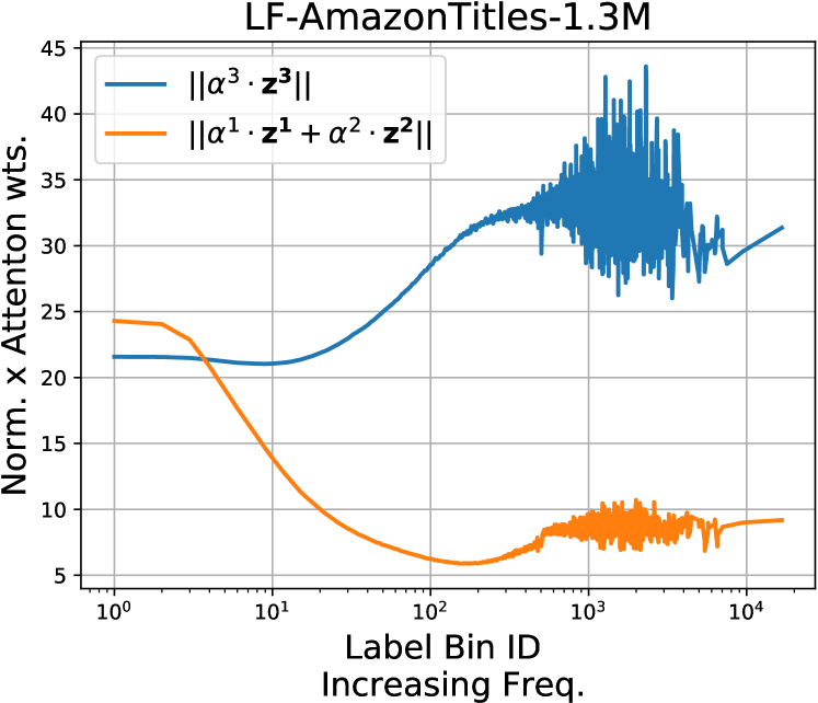
Figure 9. Analysing the dominance of various components in the label classifier ${{\mathbf{w}}}_{l}$ for rare vs popular labels. For rare labels (on the left), components that focus on label metadata i.e. $\hat{{\mathbf{z}}}^{1}_{l},\hat{{\mathbf{z}}}^{2}_{l}$ gain significance whereas for popular labels (on the right), the unrestricted refinement vector $\hat{{\mathbf{z}}}^{3}_{l}$ becomes dominant. This illustrates the importance of graph augmentation for data-scarce labels for which the refinement vectors cannot be trained adequately owing to lack of training data.

Table 6. A subjective comparison of the top 5 label predictions by ECLARE and other algorithms on the WikiSeeAlso-350K and P2PTitles-2M datasets. Predictions typeset in black color were a part of the ground truth whereas those in light gray color were not. ECLARE is able to offer precise recommendations for extremely rare labels missed by other methods. For instance, the label “Dog of Osu” in the first example is so rare that it occurred only twice in the training set. This label does not have any token overlaps with its document or co-occurring labels either. This may have caused techniques such as DECAF that rely solely on label text, to miss such predictions. The examples also establish that incorporating label co-occurrence allows ECLARE to infer the correct intent of a document or a user query. For instance, in the second example, all other methods, including DECAF, either incorrectly focus on the tokens “Academy Awards” in the document title and start predicting labels related to other editions of the Academy Awards, or else amorphous labels about entertainment awards in general. On the other hand, ECLARE is able to correctly predict other labels corresponding to award ceremonies held in the same year as the 85th Academy awards, as well as the rare label “List of …Best Foreign Language Film”. Similarly, in the third example, ECLARE correctly determines that the user is interested in faux fur coats and not necessarily in the brand Draper’s & Damon’s itself whereas methods such as DECAF that rely solely on label and document text, focus on the brand name alone and start predicting shirts and jackets of the same brand which are irrelevant to the user query.

Algorithm	Predictions
LF-WikiSeeAlsoTitles-320K
Document	Tibetan Terrier
ECLARE	Tibetan Spaniel, Tibetan kyi apso, Lhasa Apso, Dog of Osu, Tibetan Mastiff
DECAF	Fox Terrier, Tibetan Spaniel, Terrier, Bull Terrier, Bulldog
Astec	Standard Tibetan, List of domesticated Scottish breeds, List of organizations of Tibetans in exile, Tibet, Riwoche horse
Parabel	Tibet, List of organizations of Tibetans in exile, List of domesticated Scottish breeds, History of Tibet, Languages of Bhutan
AttentionXML	List of organizations of Tibetans in exile, List of domesticated Scottish breeds, Dog, Bull Terrier, Dog crossbreed
Document	85th Academy Awards
ECLARE	List of submissions to the 85th Academy Awards for Best Foreign Language Film, 33rd Golden Raspberry Awards, 19th Screen Actors Guild Awards, 67th Tony Awards, 70th Golden Globe Awards
DECAF	List of American films of 1956, 87th Academy Awards, List of American films of 1957, 1963 in film, 13th Primetime Emmy Awards
Astec	65th Tony Awards, 29th Primetime Emmy Awards, 32nd Golden Raspberry Awards, 64th Primetime Emmy Awards, 18th Screen Actors Guild Awards
Parabel	1928 in film, 1931 in film, 1930 in film, 48th Academy Awards, 26th Primetime Emmy Awards, 31st European Film Awards
AttentionXML	29th Primetime Emmy Awards, 62nd British Academy Film Awards, 60th Primetime Emmy Awards, 65th Tony Awards, 29th Golden Raspberry Awards
P2PTitles-2M
Document	Draper’s & Damon’s Women’s Chevron Faux Fur Coat Tan L
ECLARE	Grey Wolf Faux Fur Coat XXL / Grey, Big on Dots Faux-Fur Coat by LUXE, Avec Les Filles Bonded Faux-Fur Long Coat Size Large Black, Roaman’s Women’s Short Faux-Fur Coat (Black) 1X, Dennis Basso Faux Fur Jacket with Stand Collar Size XX-Small Cappuccino
DECAF	Draper’s & Damon’s Women’s Petite Cabana Big Shirt Blue P-L, Draper’s & Damon’s Women’s Petite Top It Off Stripe Jacket Blue P-L, Draper’s & Damon’s Women’s Petite Standing Ovation Jacket Black P-L, Draper & Damon Jackets & Coats | Draper & Damons Size L Colorful Coat Wpockets | Color: Black/Green | Size: L, Draper’s & Damon’s Women’s Impressionist Textured Jacket Multi L
Astec	Draper’s & Damon’s Women’s Petite Cabana Big Shirt Blue P-L, Draper’s & Damon’s Women’s Petite Top It Off Stripe Jacket Blue P-L, Draper’s & Damon’s Women’s Impressionist Textured Jacket Multi L, Draper’s & Damon’s Women’s Embroidered Tulle Jacket Dress Blue 14, Draper’s & Damon’s Women’s Petite Standing Ovation Jacket Black P-L
Parabel	Draper’s & Damon’s Women’s Impressionist Textured Jacket Multi L, Draper’s & Damon’s Women’s Over The Rainbow Jacket Multi P-L, Draper’s & Damon’s Women’s Petite Painted Desert Jacket White P-M, Draper Women’s Drapers & Damons Pants Suit - Pant Suit | Color: Black | Size: L, Draper’s & Damon’s Women’s Petite Floral & Stripe Knit Mesh Jacket Scarlet Multi P-L

Table 7. An ablation study showing loss of mutual information (lower is better) using various clustering strategies as well as fanouts. Lowering the number of metalabels $K=\left\lvert{{\mathcal{C}}}\right\rvert$ hurts performance. Competing methods that do not use graph-augmented clustering offer poor LMI, especially MACH that uses random hashes to cluster labels.

Dataset	ECLARE	ECLARE	DECAF	MACH
	$|{\mathcal{C}}|=2^{17}$	$|{\mathcal{C}}|=2^{15}$
LF-AmazonTitles-131K	5.44	5.82	7.40	29.68
LF-WikiSeeAlsoTitles-320K	3.96	11.31	5.47	35.31

Analysis. This section critically analyzes ECLARE’s performance gains by scrutinizing the following components:

1. Clustering: As is evident from Fig 8, ECLARE’s offers significantly better clustering quality. Other methods such as DECAF use label centroids over an incomplete ground truth, resulting in clusters of seemingly unrelated labels. For e.g. the label “Bulldog” was clustered with “Great house at Sonning” by DECAF and the label “Dog of Osu” was clustered with “Ferdinand II of Aragon” which never co-occur in training. However ECLARE clusters much more relevant labels together, possibly since it was able to (partly) complete the ground truth using it’s label correlation graph ${{\mathbf{G}}}$. This was also verified quantitatively by evaluating the clustering quality using the standard Loss of Mutual Information metric (LMI) (Dhillon et al., 2003). Tab 7 shows that ECLARE has the least LMI compared to other methods such as DECAF and those such as MACH that use random hashes to cluster labels.

2. Component Contribution: ECLARE chooses to dynamically attend on multiple (and heterogeneous) label representations in its classifier components, which allows it to capture nuanced variations in the semantics of each label. To investigate the contribution of the label text and refinement classifiers, Fig. 9 plots the average product of the attention weight and norm of each component. It was observed that the label text components LTE and GALE are crucial for rare labels whereas the (extreme) refinement vector $\hat{{\mathbf{z}}}^{3}_{l}$ is more important for data-abundant popular labels.

3. Label Text Augmentation: For the document “Tibetan Terrier”, ECLARE could make correct rare label predictions like “Dog of Osu” even when the label text exhibits no token similarity with the document text or other co-occurring labels. Other methods such as DECAF failed to understand the semantics of the label and mis-predicted the label “Fox Terrier” wrongly relying on the token “Terrier”. We attribute this gain to ECLARE’s label correlation graph as “Dog of Osu” correlated well with the labels “Tibetan Spaniel”, “Tibetan kyi apso” and “Tibetan Mastiff” in ${{\mathbf{G}}}$. Several such examples exist in the datasets. In another example from the P2P-2M dataset, for the product “Draper’s & Damon’s Women’s Chevron Fauz Fur Coat Tan L”, ECLARE could deduce the intent of purchasing “Fur Coat” while other XC methods incorrectly fixated on the brand “Draper’s & Damon’s”. Please refer to Tab 6 for detailed examples.

5. Conclusion

This paper presents the architecture and accompanying training and prediction techniques for the ECLARE method to perform extreme multi-label classification at the scale of millions of labels. The specific contributions of ECLARE include a framework for incorporating label graph information at massive scales, as well as critical design and algorithmic choices that enable collaborative learning using label correlation graphs with millions of labels. This includes systematic augmentations to standard XC algorithmic operations such as label-clustering, negative sampling, shortlisting, and re-ranking, to incorporate label correlations in a manner that scales to tasks with millions of labels, all of which were found to be essential to the performance benefits offered by ECLARE. The creation of label correlation graphs from ground truth data alone and its use in a GCN-style architecture to obtain multiple label representations is critical to ECLARE’s performance benefits. The proposed approach greatly outperforms state-of-the-art XC methods on multiple datasets while still offering millisecond level prediction times even on the largest datasets. Thus, ECLARE establishes a standard for incorporating label metadata into XC techniques. These findings suggest promising directions for further study including effective graph pruning for heavy tailed datasets, using higher order convolutions ($k>1$) in a scalable manner, and performing collaborative learning with heterogeneous and even multi-modal label sets. This has the potential to enable generalisation to settings where labels include textual objects such as (related) webpages and documents, but also videos, songs, etc.

- (1)
- Babbar and Schölkopf (2017) R. Babbar and B. Schölkopf. 2017. DiSMEC: Distributed Sparse Machines for Extreme Multi-label Classification. In WSDM.
- Babbar and Schölkopf (2019) R. Babbar and B. Schölkopf. 2019. Data scarcity, robustness and extreme multi-label classification. ML (2019).
- Bhatia et al. (2016) K. Bhatia, K. Dahiya, H. Jain, A. Mittal, Y. Prabhu, and M. Varma. 2016. The extreme classification repository: Multi-label datasets and code. http://manikvarma.org/downloads/XC/XMLRepository.html
- Bhatia et al. (2015) K. Bhatia, H. Jain, P. Kar, M. Varma, and P. Jain. 2015. Sparse Local Embeddings for Extreme Multi-label Classification. In NIPS.
- Bojanowski et al. (2017) P. Bojanowski, E. Grave, A. Joulin, and T. Mikolov. 2017. Enriching Word Vectors with Subword Information. Transactions of the Association for Computational Linguistics (2017).
- Chang et al. (2020) W-C. Chang, H.-F. Yu, K. Zhong, Y. Yang, and I. Dhillon. 2020. Taming Pretrained Transformers for Extreme Multi-label Text Classification. In KDD.
- Chung (2005) F. Chung. 2005. Laplacians and the Cheeger inequality for directed graphs. Annals of Combinatorics 9, 1 (2005), 1–19.
- Dahiya et al. (2021) K. Dahiya, D. Saini, A. Mittal, A. Shaw, K. Dave, A. Soni, H. Jain, S. Agarwal, and M. Varma. 2021. DeepXML: A Deep Extreme Multi-Label Learning Framework Applied to Short Text Documents. In WSDM.
- Dhillon et al. (2003) I. S. Dhillon, S. Mallela, and R. Kumar. 2003. A Divisive Information-Theoretic Feature Clustering Algorithm for Text Classification. JMLR 3 (2003), 1265–1287.
- Guo et al. (2019) C. Guo, A. Mousavi, X. Wu, Daniel N. Holtmann-Rice, S. Kale, S. Reddi, and S. Kumar. 2019. Breaking the Glass Ceiling for Embedding-Based Classifiers for Large Output Spaces. In Neurips.
- Gupta et al. (2019) V. Gupta, R. Wadbude, N. Natarajan, H. Karnick, P. Jain, and P. Rai. 2019. Distributional Semantics Meets Multi-Label Learning. In AAAI.
- Hamilton et al. (2017) W. Hamilton, Z. Ying, and J. Leskovec. 2017. Inductive representation learning on large graphs. In NIPS. 1024–1034.
- He et al. (2015) K. He, X. Zhang, S. Ren, and J. Sun. 2015. Delving deep into rectifiers: Surpassing human-level performance on imagenet classification. In Proceedings of the IEEE international conference on computer vision. 1026–1034.
- He et al. (2020) X. He, K. Deng, X. Wang, Y. Li, Y. Zhang, and M. Wang. 2020. LightGCN: Simplifying and Powering Graph Convolution Network for Recommendation. In Proceedings of the 43rd International ACM SIGIR Conference on Research and Development in Information Retrieval (SIGIR ’20).
- Jain et al. (2019) H. Jain, V. Balasubramanian, B. Chunduri, and M. Varma. 2019. Slice: Scalable Linear Extreme Classifiers trained on 100 Million Labels for Related Searches. In WSDM.
- Jain et al. (2016) H. Jain, Y. Prabhu, and M. Varma. 2016. Extreme Multi-label Loss Functions for Recommendation, Tagging, Ranking and Other Missing Label Applications. In KDD.
- Jain et al. (2017) V. Jain, N. Modhe, and P. Rai. 2017. Scalable Generative Models for Multi-label Learning with Missing Labels. In ICML.
- Jalan and Kar (2019) A. Jalan and P. Kar. 2019. Accelerating Extreme Classification via Adaptive Feature Agglomeration. IJCAI (2019).
- Jasinska et al. (2016) K. Jasinska, K. Dembczynski, R. Busa-Fekete, K. Pfannschmidt, T. Klerx, and E. Hullermeier. 2016. Extreme F-measure Maximization using Sparse Probability Estimates. In ICML.
- Joulin et al. (2017) A. Joulin, E. Grave, P. Bojanowski, and T. Mikolov. 2017. Bag of Tricks for Efficient Text Classification. In Proceedings of the European Chapter of the Association for Computational Linguistics.
- Kanagal et al. (2012) Bhargav Kanagal, Amr Ahmed, Sandeep Pandey, Vanja Josifovski, Jeff Yuan, and Lluis Garcia-Pueyo. 2012. Supercharging Recommender Systems Using Taxonomies for Learning User Purchase Behavior. VLDB (June 2012).
- Khandagale et al. (2019) S. Khandagale, H. Xiao, and R. Babbar. 2019. Bonsai - Diverse and Shallow Trees for Extreme Multi-label Classification. CoRR (2019).
- Kingma and Ba (2014) P. D. Kingma and J. Ba. 2014. Adam: A Method for Stochastic Optimization. CoRR (2014).
- Kipf and Welling (2017) T. N. Kipf and M. Welling. 2017. Semi-Supervised Classification with Graph Convolutional Networks. In 5th International Conference on Learning Representations, ICLR 2017, Toulon, France, April 24-26, 2017, Conference Track Proceedings.
- Klicpera et al. (2018) J. Klicpera, A. Bojchevski, and S. Günnemann. 2018. Predict then Propagate: Graph Neural Networks meet Personalized PageRank. In International Conference on Learning Representations.
- Liu et al. (2017) J. Liu, W. Chang, Y. Wu, and Y. Yang. 2017. Deep Learning for Extreme Multi-label Text Classification. In SIGIR.
- Liu et al. (2019) Yinhan Liu, Myle Ott, Naman Goyal, Jingfei Du, Mandar Joshi, Danqi Chen, Omer Levy, Mike Lewis, Luke Zettlemoyer, and Veselin Stoyanov. 2019. RoBERTa: A Robustly Optimized BERT Pretraining Approach. arXiv:1907.11692.
- Medini et al. (2019) T. K. R. Medini, Q. Huang, Y. Wang, V. Mohan, and A. Shrivastava. 2019. Extreme Classification in Log Memory using Count-Min Sketch: A Case Study of Amazon Search with 50M Products. In Neurips.
- Menon et al. (2011) Aditya Krishna Menon, Krishna-Prasad Chitrapura, Sachin Garg, Deepak Agarwal, and Nagaraj Kota. 2011. Response Prediction Using Collaborative Filtering with Hierarchies and Side-Information. In KDD.
- Mikolov et al. (2013) T. Mikolov, I. Sutskever, K. Chen, G. Corrado, and J. Dean. 2013. Distributed Representations of Words and Phrases and Their Compositionality. In NIPS.
- Mittal et al. (2021) A. Mittal, K. Dahiya, S. Agrawal, D. Saini, S. Agarwal, P. Kar, and M. Varma. 2021. DECAF: Deep Extreme Classification with Label Features. In WSDM.
- Miyato et al. (2018) T. Miyato, T. Kataoka, M. Koyama, and Y. Yoshida. 2018. Spectral Normalization for Generative Adversarial Networks. In ICLR.
- Niculescu-Mizil and Abbasnejad (2017) A. Niculescu-Mizil and E. Abbasnejad. 2017. Label Filters for Large Scale Multilabel Classification. In AISTATS.
- Pal et al. (2020) A. Pal, C. Eksombatchai, Y. Zhou, B. Zhao, C. Rosenberg, and J. Leskovec. 2020. PinnerSage: Multi-Modal User Embedding Framework for Recommendations at Pinterest. In KDD ’20 (Virtual Event, CA, USA) (KDD ’20). Association for Computing Machinery, New York, NY, USA, 2311–2320. https://doi.org/10.1145/3394486.3403280
- Prabhu et al. (2018a) Y. Prabhu, A. Kag, S. Gopinath, K. Dahiya, S. Harsola, R. Agrawal, and M. Varma. 2018a. Extreme multi-label learning with label features for warm-start tagging, ranking and recommendation. In WSDM.
- Prabhu et al. (2018b) Y. Prabhu, A. Kag, S. Harsola, R. Agrawal, and M. Varma. 2018b. Parabel: Partitioned label trees for extreme classification with application to dynamic search advertising. In WWW.
- Prabhu and Varma (2014) Y. Prabhu and M. Varma. 2014. FastXML: A Fast, Accurate and Stable Tree-classifier for eXtreme Multi-label Learning. In KDD.
- Sachdeva et al. (2018) Noveen Sachdeva, Kartik Gupta, and Vikram Pudi. 2018. Attentive Neural Architecture Incorporating Song Features for Music Recommendation. In RecSys.
- Schuster and Nakajima (2012) M. Schuster and K. Nakajima. 2012. Japanese and korean voice search. In 2012 IEEE International Conference on Acoustics, Speech and Signal Processing (ICASSP). IEEE, 5149–5152.
- Siblini et al. (2018) W. Siblini, P. Kuntz, and F. Meyer. 2018. CRAFTML, an Efficient Clustering-based Random Forest for Extreme Multi-label Learning. In ICML.
- Tagami (2017) Y. Tagami. 2017. AnnexML: Approximate Nearest Neighbor Search for Extreme Multi-label Classification. In KDD.
- Tang et al. (2020) P. Tang, M. Jiang, B. Xia, J. W. Pitera, Welser J., and N. V. Chawla. 2020. Multi-Label Patent Categorization with Non-Local Attention-Based Graph Convolutional Network. In AAAI, 2020.
- Velićković et al. (2018) P. Velićković, G. Cucurull, A. Casanova, A. Romero, P. Liò, and Y. Bengio. 2018. Graph Attention Networks. ICLR (2018).
- Wydmuch et al. (2018) M. Wydmuch, K. Jasinska, M. Kuznetsov, R. Busa-Fekete, and K. Dembczynski. 2018. A no-regret generalization of hierarchical softmax to extreme multi-label classification. In NIPS.
- Yen et al. (2017) E.H. I. Yen, X. Huang, W. Dai, I. Ravikumar, P.and Dhillon, and E. Xing. 2017. PPDSparse: A Parallel Primal-Dual Sparse Method for Extreme Classification. In KDD.
- Yen et al. (2016) E.H. I. Yen, X. Huang, K. Zhong, P. Ravikumar, and I. S. Dhillon. 2016. PD-Sparse: A Primal and Dual Sparse Approach to Extreme Multiclass and Multilabel Classification. In ICML.
- Yen et al. (2018) I. Yen, S. Kale, F. Yu, D. Holtmann R., S. Kumar, and P. Ravikumar. 2018. Loss Decomposition for Fast Learning in Large Output Spaces. In ICML.
- Ying et al. (2018) R. Ying, R. He, K. Chen, P. Eksombatchai, W. Hamilton, and J. Leskovec. 2018. Graph convolutional neural networks for web-scale recommender systems. In Proceedings of the 24th ACM SIGKDD International Conference on Knowledge Discovery & Data Mining. 974–983.
- You et al. (2018) R. You, S. Dai, Z. Zhang, H. Mamitsuka, and S. Zhu. 2018. AttentionXML: Extreme Multi-Label Text Classification with Multi-Label Attention Based Recurrent Neural Networks. CoRR (2018).
- Yu et al. (2014) H. Yu, P. Jain, P. Kar, and I. S. Dhillon. 2014. Large-scale Multi-label Learning with Missing Labels. In ICML.
- Zhang et al. (2020) Z. Zhang, P. Cui, and W. Zhu. 2020. Deep learning on graphs: A survey. IEEE Transactions on Knowledge and Data Engineering (2020).