Nonlinearities of King’s plot and their dependence on nuclear radii

Abstract

Investigations of isotope shifts of atomic spectral lines provide insights into nuclear properties. Deviations from the linear dependence of the isotope shifts of two atomic transitions on nuclear parameters, leading to a nonlinearity of the so-called King plot, are actively studied as a possible way of searching for the new physics. In the present work we calculate the King-plot nonlinearities originating from the Standard-Model atomic theory. The calculation is performed both analytically, for a model example applicable for an arbitrary atom, and numerically, for one-electron ions. It is demonstrated that the Standard-Model predictions of the King-plot nonlinearities are hypersensitive to experimental errors of nuclear charge radii. This effect significantly complicates identifications of possible King-plot nonlinearities originating from the new physics.

Introduction.— Introduced by W. H. King in 1963 king:63 , the King plot has been widely used as an extremely useful tool for interpreting results of the isotope-shifts atomic experiments. After measuring energies of two transitions for four or more isotopes of the same element, one can arrange the results as a King plot, which should be – to a very high accuracy – linear. In this way the experimental results can be cross-checked without any further theoretical input. Moreover, the two parameters of the linear plot can be interpreted in terms of the mass and field shifts and separately compared with theoretical calculations king:84 .

Progress in quantum logic techniques and collinear spectroscopy achieved during the last years resulted in a dramatic increase of the experimental accuracy. In particular, measurements of optical-clock transitions were demonstrated on a few-Hertz precision level knollmann:19 ; solaro:20 . Even higher accuracy can be achieved by using entangled states manovitz:19 and coherent high-resolution optical spectroscopy micke:20 . Naturally, a question arises if the King plot is going to stay linear at this new level of experimental precision. The recent experiments in strontium and ytterbium ions miyake:19 ; counts:20 gave first indications that the linearity is actually broken on the level of several standard deviations.

It was recently demonstrated frigiuele:17 ; berengut:18 ; berengut:20 that the linearity of the King plot can be used in searches for new physics, specifically, to constrain the coupling strength of hypothetical new-physics boson fields to electrons and neutrons. It remained unclear, however, whether any actually observed nonlinearity can be clearly interpreted as a manifestation of new physics, since the Standard-Model theory can also produce effects that slightly bend the King plot. Such nonlinear effects have been a subject of several recent studies flambaum:18 ; flambaum:19 ; yerokhin:20:kingsplot .

The King plot is defined so that its construction does not require any knowledge about the nuclear charge radii; only the nuclear masses are involved. Any prediction of King-plot nonlinearities, however, requires an experimental input in the form of nuclear radii. One might assumed that in view of the extreme smallness of the nonlinearities, our limited knowledge of the nuclear radii should not cause any problems. In the present work we will demonstrate that it is exactly the opposite. Even very small errors in experimental nuclear radii lead to greatly amplified uncertainties of the King-plot nonlinearities, which bring about problems in asserting even the order of the magnitude of the effect. This makes the King-plot nonlinearities a very sensitive tool for studying nuclear radii, but diminish their valuableness for searches of new physics.

Arbitrary atom.— Let us consider the isotope shift of the energy of the transition $a$ between the isotopes with the mass numbers $A_{i}$ and $A_{0}$, which will be denoted as $E_{a}^{i}$ (the reference isotope $A_{0}$ will be implicit everywhere and suppressed in the notations for brevity). It is convenient to introduce the so-called reduced isotope-shift energies $n_{a}^{i}$ as

$$n_{a}^{i}=\frac{E_{a}^{i}}{\nicefrac{{m}}{{M_{i}}}-\nicefrac{{m}}{{M_{0}}}}\,,$$ (1)

where $m$ is the electron mass and $M_{k}$ is the nuclear mass of the isotope $A_{k}$. Within the standard formulation, the reduced isotope-shift energy is represented as a sum of the mass-shift and the field-shift contributions,

$$n_{a}^{i}=K_{a}+F_{a}\,r^{(2)}_{i}\,,$$ (2)

where $K_{a}$ and $F_{a}$ are the mass-shift and the field-shift constants, respectively, $r^{(2)}_{i}\equiv\left[\nicefrac{{R^{2}_{i}}}{{\lambdabar_{C}^{2}}}-\nicefrac{{R^{2}_{0}}}{{\lambdabar_{C}^{2}}}\right]/\left[\nicefrac{{m}}{{M_{i}}}-\nicefrac{{m}}{{M_{0}}}\right]$, $R_{k}$ is the root-mean-square (rms) nuclear charge radius of the isotope $A_{k}$, and $\lambdabar_{C}=\nicefrac{{\lambda_{C}}}{{2\pi}}$ is the reduced Compton wavelength.

It is usually assumed that the isotope-shift constants $K_{a}$ and $F_{a}$ depend only on the transition but not on the isotope. In this case, by considering two transitions, $a$ and $b$, and three pairs of isotopes $(A_{i},A_{0})$ with $i=1$, 2, and 3, one can form the so-called King’s plot king:63 . It is easy to show that three points $(x_{i},y_{i})=(n_{a}^{1},n_{b}^{1}),(n_{a}^{2},n_{b}^{2}),(n_{a}^{3},n_{b}^{3})$ lie on a straight line,

$$y=\Big{(}K_{b}-\frac{F_{b}}{F_{a}}\,K_{a}\Big{)}+\frac{F_{b}}{F_{a}}\,x\,.$$ (3)

It is important that the linear dependence of $(n_{a}^{i},n_{b}^{i})$ does not rely on a theoretical knowledge of the isotope-shift constants; the only theoretical input is the representation of the isotope shifts in the form of Eq. (2). This representation is remarkably accurate, but at the level of the present-day experimental precision it may be not accurate enough.

Let us now consider a generalization of Eq. (2) that takes into account that the field-shift, in addition to $R^{2}$, depends also on a higher power of $R$. Specifically, we write

$$n_{a}^{i}=K_{a}+F_{a}\,r^{(2)}_{i}+F_{a}w_{a}r^{(3)}_{i}\,,$$ (4)

where $r^{(3)}_{i}\equiv\left[\nicefrac{{R^{3}_{i}}}{{\lambdabar_{C}^{3}}}-\nicefrac{{R^{3}_{0}}}{{\lambdabar_{C}^{3}}}\right]/\left[\nicefrac{{m}}{{M_{i}}}-\nicefrac{{m}}{{M_{0}}}\right]$ and $w_{a}$ is an additional isotope-shift constant, which depends on the transition but not on the isotope. We keep in mind that $r^{(3)}_{i}\approx(\nicefrac{{R_{0}}}{{\lambdabar_{C}}})\,r^{(2)}_{i}\ll r^{(2)}_{i}$ since $R_{0}/\lambdabar_{C}\approx 0.01$.

Obviously, the three points $(n_{a}^{i},n_{b}^{i})$ of Eq. (4) lie no longer on a straight line but rather on a parabola, $y=a+bx+cx^{2}$. The nonlinearity of this function is connected with the coefficient $c=(\nicefrac{{1}}{{2}})\,y^{\prime\prime}(x)$. Evaluating the second derivative of the exact fit of the three points $(n_{a}^{i},n_{b}^{i})$ and neglecting $r^{(3)}_{i}$ on the background of $r^{(2)}_{i}$, we arrive at the following expression

$$y^{\prime\prime}=2\,\frac{F_{b}}{F_{a}^{2}}\,(w_{a}-w_{b})\,{\cal P}_{\rm nucl}\,,$$ (5)

where

$${\cal P}_{\rm nucl}=\frac{r^{(2)}_{3}(r^{(3)}_{1}-r^{(3)}_{2})+r^{(2)}_{1}(r^{(3)}_{2}-r^{(3)}_{3})+r^{(2)}_{2}(r^{(3)}_{3}-r^{(3)}_{1})}{(r^{(2)}_{1}-r^{(2)}_{2})(r^{(2)}_{1}-r^{(2)}_{3})(r^{(2)}_{2}-r^{(2)}_{3})}\,.$$ (6)

It is now clear that if we would like to predict the nonlinearity of King’s plot in the approximation of Eq. (4), we have to calculate the field-shift constants $F_{a,b}$ and $w_{a,b}$ and multiply them by the nuclear factor ${\cal P}_{\rm nucl}$, which is determined by the experimental nuclear parameters (charge radii and masses) of the isotopes.

Let us now address the question: to which accuracy can we determine the nuclear factor ${\cal P}_{\rm nucl}$ basing on the available experimental data? We consider an example of four isotopes of tin ($Z=50$) with $A_{i}=(118,120,122,124)$. The nuclear radii are taken angeli:13 as $R_{118}=4.6393\,(1)$ fm, $R_{120}=4.6519$ fm, $R_{122}=4.6634\,(1)$ fm, and $R_{124}=4.6735\,(1)$ fm. Note that we keep only the relative uncertainty of the radii with respect to the $A=120$ isotope, omitting the common systematic uncertainty of 0.0020 fm, which will be ignored in the present context. The nuclear masses are taken from Ref. wang:12 ; their uncertainties do not play any role here.

We now evaluate ${\cal P}_{\rm nucl}$ numerically, varying each of $R_{i}$ within their uncertainties. The result is surprising: although the nuclear radii are supposed to be known with a five-digit accuracy, the results for ${\cal P}_{\rm nucl}$ may vary by several orders of magnitude! Specifically, we obtain $|{\cal P}_{\rm nucl,min}|=5.6\times 10^{-5}$ and $|{\cal P}_{\rm nucl,max}|=1.3\times 10^{-3}$. The reason for such striking behaviour is that both the numerator and the denominator in Eq. (6) can nearly vanish for some combinations of $R_{i}$, leading to very small or very large values of ${\cal P}_{\rm nucl}$.

We have to conclude that regardless of the accuracy of theoretical calculations of the isotope-shift constants, any predictions for the nonlinearities of the King plot are problematic because of their extreme sensitivity to errors of experimental nuclear radii. A way to circumvent this problem might be to consider the ratio of the nonlinearities for two pairs of transitions. We note that in Eq. (5) the nuclear part is factorized out and, therefore, the ratio of the second derivatives $y^{\prime\prime}$ for two pairs of transitions is free from the nuclear uncertainties. However, the exact factorization holds only for one-parameter extensions of the standard formula like Eq. (4).

The realistic situation is more complicated. In particular, the field-shift constant contains terms with $\ln R$ in its expansion and is modified by the nuclear-polarization effects which often demonstrate irregular dependence on the isotope mass number. The general expression for the reduced isotope-shift energy can be written as

$$n_{a}^{i}=K_{a}^{i}+F_{a}^{i}\,r^{(2)}_{i}\,,$$ (7)

where the isotope-shift “constants” $K_{a}^{i}$ and $F_{a}^{i}$ depend on the isotope parameters (which is indicated by the superscript $i$). For a general atom, theoretical predictions of the isotope dependence of these constants are rather complicated. In the present work we will address this problem for the simplest case of H-like ions.

H-like ions.— We now turn to examining the case of one-electron ions. From now on, we will adopt the relativistic units with $c=\hbar=1$, which greatly simplifies the following formulas. We start with the mass shift. The main isotope dependence of the mass-shift constant comes from the quadratic part $\sim\!(\nicefrac{{m}}{{M}})^{2}$ of the nuclear recoil effect. Specifically, we write

$$K_{a}^{i}=K_{a}^{(1)}+\frac{m}{M_{i}}\,K_{a}^{(2)}\,,$$ (8)

where the first-order mass-shift constant $K^{(1)}$ is well-known, see, e.g., review yerokhin:15:Hlike , and $K^{(2)}$ is the second-order mass-shift constant calculated in the present work. For a reference state with quantum numbers $(njl)$, the second-order mass-shift constant is expressed as a second-order perturbation correction induced by the relativistic recoil operator ${H}_{\rm rec}$ shabaev:85 ,

$$K^{(2)}_{njl}=\sum_{k\neq(njl)}\frac{\langle njl|{H}_{\rm rec}|k\rangle\,\langle k|{H}_{\rm rec}|njl\rangle}{\varepsilon_{njl}-\varepsilon_{k}}\,,$$ (9)

where summation over $k$ is performed over the complete Dirac spectrum and

$${H}_{\rm rec}=\frac{1}{2}\left[{\bm{p}}^{2}-\frac{Z\alpha}{r}\left(\bm{\alpha}+\frac{(\bm{\alpha}\cdot{\bm{r}})\,{\bm{r}}}{r^{2}}\right)\cdot{\bm{p}}\right]\,.$$ (10)

Here, ${\bm{p}}$ is the electron momentum and ${\bm{\alpha}}$ is the vector of Dirac matrices. We calculate $K^{(2)}_{njl}$ in two ways: analytically, performing the summation over the Dirac spectrum with help of generalized virial relations shabaev:91:jpb , and numerically, with the finite basis set $B$-spline method shabaev:04:DKB . Results obtained by two different methods agree with each other. For light ions, we also observe good agreement with known results for the first terms of the $Z\alpha$ expansion yerokhin:15:Hlike

$$K^{(2)}_{njl}=-\frac{(Z\alpha)^{2}}{2n^{2}}+\frac{(Z\alpha)^{4}}{2n^{3}}\left(\frac{3}{2n}-\frac{2}{2l+1}\right)+\ldots\,.$$ (11)

The isotope dependence of the field-shift constant arises from two main sources: (i) the deviation of the $R$-dependence of the finite nuclear size (fns) correction from the $R^{2}$ form and (ii) the effect of the nuclear polarization. The fns correction to the energy levels $\Delta E_{\rm fns}$ is calculated numerically, by solving the Dirac equation with the potential of an extended nuclear charge, see Ref. yerokhin:11:fns for details. The obtained results are represented, factorizing out the leading $R$ dependence shabaev:93:fns , as

$$\Delta E_{\rm fns} =R^{2\gamma}\,G_{\rm fns}(Z\alpha,R)\,,$$ (12)

where $\gamma=\sqrt{(j+\nicefrac{{1}}{{2}})^{2}-(Z\alpha)^{2}}$ and $R$ is the nuclear rms radius. The field-shift constant is obtained from the fns correction to the transition energy as $F_{a}^{i}=\nicefrac{{\Delta E_{{\rm fns},a}}}{{R^{2}}}$. We note that the deviation of the $R^{2\gamma}$ term in Eq. (12) from the standard $R^{2}$ factor does not cause any nonlinearity of King’s plot, because it leads to a multiplication of $F$ in Eq. (2) by a factor that does not depend on the transition. So, the fns contribution to the nonlinearity comes only from the $R$ dependence of the function $G_{\rm fns}$. We note that this dependence is very weak; in order to reliably calculate it for medium-$Z$ ions, we had to solve the Dirac equation in the extended-precision arithmetics.

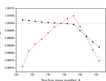
Figure 1: The isotope dependence of the finite nuclear size and nuclear polarization effects, with the leading $R^{2\gamma}$ dependence factorized out, for the $1s$ state of H-like barium ($Z=56$). Black diamonds show the finite nuclear size correction, in terms of the function $G_{\rm fns}$ defined by Eq. (12). The red circles present results for the combined nuclear size and nuclear polarization effect, in terms of the function $G_{\rm nucl}=G_{\rm fns}(1-\nicefrac{{1}}{{1000}}\,g_{\rm np})$. Both functions $G_{\rm fns}(A)$ and $G_{\rm nucl}(A)$ are normalized to their values for the isotope $A_{0}=134$.

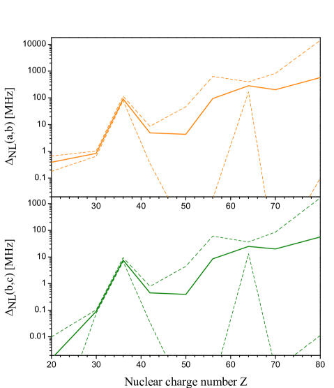
Figure 2: King-plot nonlinearities of H-like ions for two transition pairs, $(a,b)$ (top) and $(b,c)$ (bottom), where $a=1s\to 2p_{1/2}$, $b=2s\to 2p_{1/2}$, and $c=2s\to 2p_{3/2}$. The calculated points correspond to the isotope chains $(A_{0},A_{0}+2,A_{0}+4,A_{0}+6)$, with the reference ($A_{0}$) isotopes: ⁴⁰Ca, ⁶⁴Zn, ⁸²Kr, ⁹²Mo, ¹¹⁸Sn, ¹³²Ba, ¹⁵⁴Gd, ¹⁶⁶Yb, ¹⁹⁶Hg. The dashed lines represent the variation of the nonlinearities when the nuclear radii are varied within their experimental uncertainties.

The nuclear polarization correction to the energy of a state with quantum numbers $(njl)$ is expressed as plunien:95 ; nefiodov:96

$$\Delta E_{\rm np}=-\alpha\sum_{LM}B(EL)\,\sum_{k}\frac{\big{|}\langle njl|F_{L}\,Y_{LM}|k\rangle\big{|}^{2}}{\varepsilon_{k}-\varepsilon_{njl}+{\rm sign}(\varepsilon_{k})\,\omega_{L}}\,,$$ (13)

where $B(EL)=B(EL;L\to 0)$ are the reduced probabilities of nuclear transitions from the excited (“$L$”) to the ground (“$0$”) level, $\omega_{L}$ are the nuclear excitation energies with respect to the ground state, $F_{L}$ are radial functions given by Eq. (4) of Ref. nefiodov:96 , $Y_{LM}$ are the spherical harmonics, and the summation over $k$ is performed over the complete spectrum of electronic states. Multipole contributions in Eq. (13) are usually separated into two classes: contributions from the giant resonance transitions and those from the lowest-lying nuclear rotational transitions. Among the latter, the electrical quadrupole transition between the ground 0⁺ the lowest-lying 2⁺ state is the dominant channel for most of even-even nuclides. Our calculation of the nuclear polarization correction includes the dominant $E2$ nuclear rotational transition and the giant resonance transitions with $L\leq 3$. Experimental results for the nuclear quadrupole transition probabilities $B(E2)$ and excitation energies $\omega_{L}$ were taken from Ref. raman:01 . The summation over the Dirac spectrum was performed with help of the finite basis set $B$-spline method shabaev:04:DKB . We find good agreement with numerical results of Ref. nefiodov:96 . A similar calculation was recently presented in Ref. flambaum:21 ; the difference is that in that work empirical approximate formulas were used for $B(E2)$ and only the dominant $L=1$ giant resonance was included.

Numerical results of our calculation of the nuclear polarization correction are conveniently parameterized in terms of the dimensionless function $g_{\rm np}$, defined as a multiplicative factor to the fns correction,

$$\Delta E_{\rm np}=-\frac{g_{\rm np}(Z,A)}{1000}\,\Delta E_{\rm fns}\,.$$ (14)

We studied the nuclear polarization effect for the $1s$, $2s$ and $2p_{1/2}$ states; for the $2p_{3/2}$ state the corresponding correction is very small and thus neglected. We find that $g_{\rm np}$ varies from $0.3$ to $1.0$ for all nuclei encountered in the present work, $Z\in(20,92)$. It is instructive to compare the isotope dependence of the fns and the nuclear polarization effects. Such a comparison is presented in Fig. 1 for a chain of isotopes of Ba⁵⁵⁺. We observe that both effects yield significant contributions, but the nuclear polarization is larger and, more importantly, its isotope dependence is non-monotonic. This is connected with the behaviour of the nuclear transition probabilities $B(E2)$, which tend to grow as the nuclide mass number moves away from the stability region. We note that the kink of the plot for $G_{\rm fns}$ is due to unevenness of the dependence of $R$ on the mass number $A$.

We are now in position to calculate the King-plot nonlinearities for H-like ions. We adopt the definition yerokhin:20:kingsplot ; flambaum:18 of the nonlinearity of a 3-point curve as a shift of the ordinate of the third point from the straight line defined by the first two points,

$$\delta\epsilon^{3}_{ab}=\Big{(}\frac{m}{M_{3}}-\frac{m}{M_{0}}\Big{)}\left[n^{3}_{b}-n^{1}_{b}-\frac{n^{2}_{b}-n^{1}_{b}}{n^{2}_{a}-n^{1}_{a}}\left(n^{3}_{a}-n^{1}_{a}\right)\right].$$ (15)

The nonlinearity of the King plot for the transition pair $(a,b)$ is defined by symmetrizing the above expression with respect of $a$ and $b$,

$$\Delta_{\rm NL}(ab)=\nicefrac{{1}}{{2}}\left(\big{|}\delta\epsilon^{3}_{ab}\big{|}+\big{|}\delta\epsilon^{3}_{ba}\big{|}\right).$$ (16)

The nonlinearity $\Delta_{\rm NL}$ has a dimension of energy and approximately indicates the experimental accuracy needed in order to detect it. We note that the numerical evaluation of $\Delta_{\rm NL}$ involves large numerical cancellations (due to multiple subtractions of similar numbers) and needs to be performed in an extended-precision arithmetics.

Results of our numerical calculations of the King-plot nonlinearities for different H-like ions are presented in Fig. 2. We studied two pairs of transitions, $(a,b)$ and $(b,c)$, with $a=1s\to 2p_{1/2}$, $b=2s\to 2p_{1/2}$, and $c=2s\to 2p_{3/2}$. From Fig. 2 we make several conclusions which could have been anticipated from our earlier analytical considerations. First, we find that the calculated nonlinearities behave irregularly as a function of $Z$, because they crucially depend on differences of charge radii of the nuclides. Second, we find that the experimental errors of the nuclear radii cause tremendously amplified uncertainties of the resulting nonlinearities. Generally, only the upper bounds of the nonlinearities can be predicted and these bounds depend crucially on the assumed uncertainties of the nuclear radii. We would like to stress that for our analysis we selected the nuclides with the best-known charge radii. Specifically, the relative uncertainties of the rms radii for the studied nuclides with $Z>40$ are about 0.0001 fm angeli:13 . For less known isotopes, the uncertainties of nonlinearities are larger by orders of magnitude.

Although our numerical calculations were performed for the specific choice of H-like ions, we expect that the situation remains qualitatively the same for many-electron atoms, including the case of singly charged ions which are most relevant from the experimental point of view. This expectation is supported by the analytical example discussed in the first part of the present paper. In order to obtain quantitative results for the upper bounds for the Standard-Model King-plot nonlinearities for singly charged ions, dedicated calculations are needed for each particular element.

The observed hypersensitivity of the King-plot nonlinearities on the nuclear radii can be used for improving our knowledge of the isotope differences of the nuclear charge radii. For example, if one of the three differences of the nuclear radii involved in the King plot is known significantly worse than the other two, it should be possible to improve its value basing on the measured King-plot nonlinearity.

The dependence of the predicted King-plot nonlinearities on the nuclear radii can be significantly reduced if we study the ratio of the nonlinearities for two transition pairs, e.g., $\Delta_{\rm NL}(ab)/\Delta_{\rm NL}(bc)$. This can be seen from the analytical example of Eq. (5) and also from the fact that the plots for $\Delta_{\rm NL}(ab)$ and $\Delta_{\rm NL}(bc)$ in Fig. 2 look very similar. However, the factorization of the nuclear degrees of freedom, exact in the case of Eq. (5), becomes only approximate in the complete calculation. As a consequence, we still encounter combinations of nuclear radii leading to strong variations of the ratio of the nonlinearities.

Turning to perspectives of using the King-plot nonlinearities for searches of new physics beyond the Standard Model, we conclude that the findings of the present work significantly complicate such searches. More specifically, when an experiment detects a nonlinearity (as, e.g., in Refs. miyake:19 ; counts:20 ), it should be very difficult to distinguish whether this is caused by the new physics or the standard atomic theory, because of our limited knowledge of the nuclear charge radii. Therefore, the upper bounds on the new physics derived from such an observation will be defined by the observed nonlinearity and any further progress in experimental precision will not improve these bounds. An alternative approach would be to use independent constraints to eliminate the possibility of the new physics bordag:11 ; raffelt:12 ; hardy:17 ; delaunay:17 and interpret the observed nonlinearities in terms of constraints on the nuclear radii.

Summarizing, we calculated nonlinearities of the King plot originating from the Standard-Model atomic theory. The calculations were performed first analytically for a model problem applicable for an arbitrary atom. Next we performed a detailed numerical calculation for hydrogen-like ions, taking into account the quadratic nuclear recoil, the higher-order finite nuclear size and the nuclear polarization effects. We found that the Standard-Model predictions of the King-plot nonlinearities are hypersensitive to experimental errors of nuclear charge radii, often leading to uncertainties even in the order of magnitude of the effect. Our restricted knowledge of the nuclear radii leads to the greatly magnified ambiguities in the Standard-Model predictions of the nonlinearities, thus greatly complicating an identification of possible effects originating from new physics.

Acknowledgments.— The calculations for arbitrary atoms were supported by the Russian Science Foundation, Grant No. 20-62-46006. The calculations for H-like ions were supported by Deutsche Forschungsgemeinschaft through Grant No. SU 658/4-1.

References

- (1) W. H. King, J. Opt. Soc. Am. 53, 638 (1963).
- (2) W. H. King, Isotope Shifts in Atomic Spectra, Plenum Press, New York, 1984.
- (3) F. W. Knollmann, A. N. Patel, and S. C. Doret, Phys. Rev. A 100, 022514 (2019).
- (4) C. Solaro, S. Meyer, K. Fisher, J. C. Berengut, E. Fuchs, and M. Drewsen, Phys. Rev. Lett. 125, 123003 (2020).
- (5) T. Manovitz, R. Shaniv, Y. Shapira, R. Ozeri, and N. Akerman, Phys. Rev. Lett. 123, 203001 (2019).
- (6) P. Micke, T. Leopold, S. King, E. Benkler, L. Spieß, L. Schmoeger, M. Schwarz, J. C. López-Urrutia, and P. Schmidt, Nature 578, 60 (2020).
- (7) H. Miyake, N. C. Pisenti, P. K. Elgee, A. Sitaram, and G. K. Campbell, Phys. Rev. Research 1, 033113 (2019).
- (8) I. Counts, J. Hur, D. P. L. Aude Craik, H. Jeon, C. Leung, J. C. Berengut, A. Geddes, A. Kawasaki, W. Jhe, and V. Vuletić, Phys. Rev. Lett. 125, 123002 (2020).
- (9) C. Frugiuele, E. Fuchs, G. Perez, and M. Schlaffer, Phys. Rev. D 96, 015011 (2017).
- (10) J. C. Berengut, D. Budker, C. Delaunay, V. V. Flambaum, C. Frugiuele, E. Fuchs, C. Grojean, R. Harnik, R. Ozeri, G. Perez, and Y. Soreq, Phys. Rev. Lett. 120, 091801 (2018).
- (11) J. C. Berengut, C. Delaunay, A. Geddes, and Y. Soreq, Phys. Rev. Research 2, 043444 (2020).
- (12) V. Flambaum, A. Geddes, and A. Viatkina, Phys. Rev. A 97, 032510 (2018).
- (13) V. Flambaum and V. Dzuba, Phys. Rev. A 100, 032511 (2019).
- (14) V. A. Yerokhin, R. A. Müller, A. Surzhykov, P. Micke, and P. O. Schmidt, Phys. Rev. A 101, 012502 (2020).
- (15) I. Angeli and K. Marinova, At. Dat. Nucl. Dat. Tabl. 99, 69 (2013).
- (16) M. Wang, G. Audi, A. H. Wapstra, F. G. Kondev, M. MacCormick, X. Xu, and B. Pfeiffer, Chin. Phys. C 36, 1603 (2012).
- (17) V. A. Yerokhin and V. M. Shabaev, J. Phys. Chem. Ref. Data 44, 033103 (2015).
- (18) V. M. Shabaev, Theor. Math. Phys. 63, 588 (1985).
- (19) V. M. Shabaev, J. Phys. B 24, 4479 (1991).
- (20) V. M. Shabaev, I. I. Tupitsyn, V. A. Yerokhin, G. Plunien, and G. Soff, Phys. Rev. Lett. 93, 130405 (2004).
- (21) V. A. Yerokhin, Phys. Rev. A 83, 012507 (2011).
- (22) V. M. Shabaev, J. Phys. B 26, 1103 (1993).
- (23) G. Plunien and G. Soff, Phys. Rev. A 51, 1119 (1995), (E) ibid., 53, 4614 (1996).
- (24) A. V. Nefiodov, L. N. Labzowsky, G. Plunien, and G. Soff, Phys. Lett. A 222, 227 (1996).
- (25) S. Raman, C. Nestor, and P. Tikkanen, At. Dat. Nucl. Dat. Tabl. 78, 1 (2001).
- (26) V. Flambaum, I. Samsonov, H. T. Tan, and A. Viatkina, Phys. Rev. A 103, 032811 (2021).
- (27) M. Bordag, U. Mohideen, and V. Mostepanenko, Physics Reports 353, 1 (2001).
- (28) G. Raffelt, Phys. Rev. D 86, 015001 (2012).
- (29) E. Hardy and R. Lasenby, J. High Energy Phys. 2017, 33 (2017).
- (30) C. Delaunay, R. Ozeri, G. Perez, and Y. Soreq, Phys. Rev. D 96, 093001 (2017).