Abstract.
We study a free boundary problem modeling multi-layer tumor growth with a small time delay τ 𝜏 \tau ( σ ∗ , p ∗ , ρ ∗ , ξ ∗ ) subscript 𝜎 subscript 𝑝 subscript 𝜌 subscript 𝜉 (\sigma_{*},p_{*},\rho_{*},\xi_{*}) μ > 0 𝜇 0 \mu>0 μ 𝜇 \mu μ ∗ > 0 subscript 𝜇 0 \mu_{*}>0 ( σ ∗ , p ∗ , ρ ∗ , ξ ∗ ) subscript 𝜎 subscript 𝑝 subscript 𝜌 subscript 𝜉 (\sigma_{*},p_{*},\rho_{*},\xi_{*}) μ < μ ∗ 𝜇 subscript 𝜇 \mu<\mu_{*} μ > μ ∗ 𝜇 subscript 𝜇 \mu>\mu_{*}
Keywords.
Free boundary problem; Tumor model; Stability; Time-delay
2010 mathematics subject classifications. 35R35, 35K57, 35B40, 92B05
1. Introduction
There is a variety of shapes of tumors in tissue cultures. It is known that three-dimensional tumors grown in tissue culture are likely to take the shape of spheroids; a large number of partial differential equation (PDE) sphere-shaped tumors models have been developed, and a variety of properties including
well-posedness, asymptotic stability, bifurcation, the impact of a variety of biological relevant parameters, etc., are studied. For example, the first model of free boundary problem for a solid tumor growth is proposed and analyzed by Greenspan in [12 ] and [13 ] . In
[11 ] , Friedman and Reitich considered global well-posedness and global asymptotically stability for radially symmetric solutions.
For the non-symmetric case, Bazaliy
and Friedman established the local well-posedness and asymptotic behavior under non-radial perturbations for the time-dependent problem in [2 ] and [1 ] . In particular, Friedman and Hu extended the work by giving a precise threshold in [8 ] .
For more details,
we refer to the papers [9 , 10 , 18 ] and the references therein.
Medico-biologists have recently developed that cellular aggregates gather on permeable membranes, causing them to form multilayered tumor cell.
Because multilayered tumor cells are grown on permeable membranes which can separate two reservoirs of the diffusion apparatus directly, it is an important task to study the fluidity of drug and metabolism of tumor tissue.
See [16 , 17 , 14 , 15 ] for the study of multilayered tumor cells.
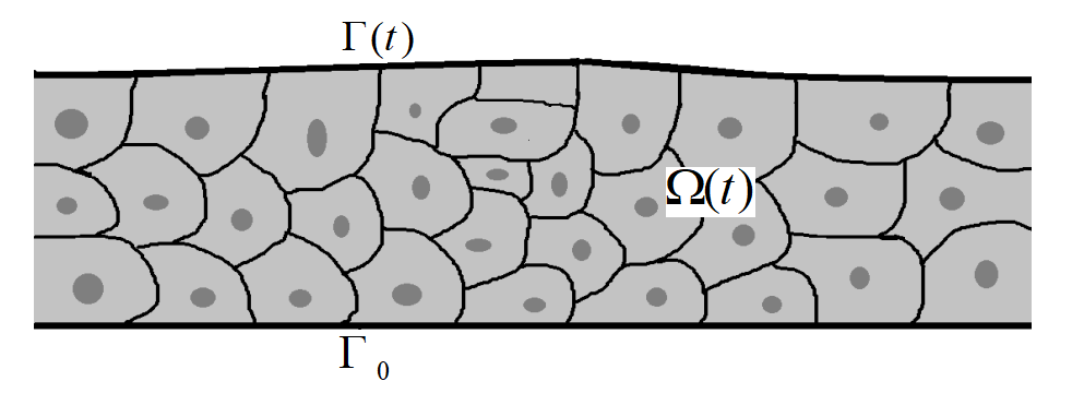
Following the works of Cui and Escher [5 ] and Zhou, Escher and Cui [24 ] , we consider in this paper the following 3-dimensional multilayered tumor region of the flat-shaped form
Ω ( t ) ≜ { ( x , y ) ∈ ℝ 2 × ℝ ; 0 < y < ρ ( t , x ) } , 𝐱 = ( x , y ) = ( x 1 , x 2 , y ) , formulae-sequence ≜ Ω 𝑡 formulae-sequence 𝑥 𝑦 superscript ℝ 2 ℝ 0 𝑦 𝜌 𝑡 𝑥 𝐱 𝑥 𝑦 subscript 𝑥 1 subscript 𝑥 2 𝑦 \Omega(t)\triangleq\{(x,y)\in{\mathbb{R}}^{2}\times{\mathbb{R}};\;\;0<y<\rho(t,x)\},\hskip 20.00003pt{\bf x}=(x,y)=(x_{1},x_{2},y),
where ρ ( t , x ) 𝜌 𝑡 𝑥 \rho(t,x) Γ ( t ) Γ 𝑡 \Gamma(t) { y = ρ ( t , x ) } 𝑦 𝜌 𝑡 𝑥 \{y=\rho(t,x)\} Ω ( t ) Ω 𝑡 \Omega(t)
Figure 1.
Through the upper boundary Γ ( t ) Γ 𝑡 \Gamma(t) σ 𝜎 \sigma σ 𝜎 \sigma λ σ t − Δ σ + σ = 0 𝜆 subscript 𝜎 𝑡 Δ 𝜎 𝜎 0 \lambda\sigma_{t}-\Delta\sigma+\sigma=0 λ 𝜆 \lambda λ = 0 𝜆 0 \lambda=0
For simplicity, we assume that the tumor is immersed in an environment with nutrient concentration σ ¯ ¯ 𝜎 \overline{\sigma} Γ 0 subscript Γ 0 \Gamma_{0} { y = 0 } 𝑦 0 \{y=0\} Γ 0 subscript Γ 0 \Gamma_{0}
(1.1) − Δ σ + σ = 0 , ( x 1 , x 2 , y ) ∈ Ω ( t ) , t > 0 , formulae-sequence Δ 𝜎 𝜎 0 formulae-sequence subscript 𝑥 1 subscript 𝑥 2 𝑦 Ω 𝑡 𝑡 0 \displaystyle-\Delta\sigma+\sigma=0,\hskip 20.00003pt(x_{1},x_{2},y)\in\Omega(t),\hskip 20.00003ptt>0,
(1.2) σ = σ ¯ , ( x 1 , x 2 , y ) ∈ Γ ( t ) , t > 0 , formulae-sequence 𝜎 ¯ 𝜎 formulae-sequence subscript 𝑥 1 subscript 𝑥 2 𝑦 Γ 𝑡 𝑡 0 \displaystyle\sigma=\overline{\sigma},\hskip 20.00003pt(x_{1},x_{2},y)\in\Gamma(t),\hskip 20.00003ptt>0,
(1.3) ∂ σ ∂ y = 0 , ( x 1 , x 2 , y ) ∈ Γ 0 , t > 0 . formulae-sequence 𝜎 𝑦 0 formulae-sequence subscript 𝑥 1 subscript 𝑥 2 𝑦 subscript Γ 0 𝑡 0 \displaystyle\displaystyle\frac{\partial\sigma}{\partial y}=0,\hskip 20.00003pt(x_{1},x_{2},y)\in\Gamma_{0},\hskip 20.00003ptt>0.
If the tumor is assumed to be of porous medium type where Darcy’s law (i.e., V → = − ∇ p → 𝑉 ∇ 𝑝 \vec{V}=-\nabla p p 𝑝 p div V → = S div → 𝑉 𝑆 \mbox{div}\vec{V}=S S 𝑆 S
The proliferation rate S 𝑆 S σ − σ ~ 𝜎 ~ 𝜎 \sigma-\widetilde{\sigma} σ ~ ~ 𝜎 \widetilde{\sigma} τ 𝜏 \tau S = μ [ σ ( ξ ( t − τ ; 𝐱 , t ) , t − τ ) − σ ~ ] 𝑆 𝜇 delimited-[] 𝜎 𝜉 𝑡 𝜏 𝐱 𝑡
𝑡 𝜏 ~ 𝜎 S=\mu[\sigma(\xi(t-\tau;{\bf x},t),t-\tau)-\widetilde{\sigma}] μ 𝜇 \mu ξ ( s ; 𝐱 , t ) 𝜉 𝑠 𝐱 𝑡
\xi(s;{\bf x},t) s 𝑠 s 𝐱 = ( x 1 , x 2 , y ) 𝐱 subscript 𝑥 1 subscript 𝑥 2 𝑦 {\bf x}=(x_{1},x_{2},y) t 𝑡 t V → = − ∇ p → 𝑉 ∇ 𝑝 \vec{V}=-\nabla p
(1.4) d ξ ( s ; 𝐱 , t ) d s = − ∇ p ( ξ ( s ; 𝐱 , t ) , s ) , t − τ ≤ s ≤ t , formulae-sequence d 𝜉 𝑠 𝐱 𝑡
d 𝑠 ∇ 𝑝 𝜉 𝑠 𝐱 𝑡
𝑠 𝑡 𝜏 𝑠 𝑡 \displaystyle\displaystyle\frac{\mathrm{d}\xi(s;{\bf x},t)}{\mathrm{d}s}=-\nabla p({\xi(s;{\bf x},t),s)},\hskip 20.00003ptt-\tau\leq s\leq t,
(1.5) ξ ( s ; x 1 , x 2 , y , t ) = ( x 1 , x 2 , y ) , s = t . formulae-sequence 𝜉 𝑠 subscript 𝑥 1 subscript 𝑥 2 𝑦 𝑡
subscript 𝑥 1 subscript 𝑥 2 𝑦 𝑠 𝑡 \displaystyle\xi(s;x_{1},x_{2},y,t)=(x_{1},x_{2},y),\hskip 20.00003pts=t.
Combining the expression of S 𝑆 S
(1.6) − Δ p = μ [ σ ( ξ ( t − τ ; x 1 , x 2 , y , t ) , t − τ ) − σ ~ ] , ( x 1 , x 2 , y ) ∈ Ω ( t ) , t > 0 , formulae-sequence Δ 𝑝 𝜇 delimited-[] 𝜎 𝜉 𝑡 𝜏 subscript 𝑥 1 subscript 𝑥 2 𝑦 𝑡
𝑡 𝜏 ~ 𝜎 formulae-sequence subscript 𝑥 1 subscript 𝑥 2 𝑦 Ω 𝑡 𝑡 0 -\Delta p=\mu[\sigma(\xi(t-\tau;x_{1},x_{2},y,t),t-\tau)-\widetilde{\sigma}],\hskip 20.00003pt(x_{1},x_{2},y)\in\Omega(t),\hskip 20.00003ptt>0,
and assuming the velocity field is continuous up to the boundary, the normal velocity of the moving boundary Γ ( t ) Γ 𝑡 \Gamma(t)
(1.7) V n = − ∇ p ⋅ n = − ∂ p ∂ n , ( x 1 , x 2 , y ) ∈ Γ ( t ) , t > 0 . formulae-sequence subscript 𝑉 𝑛 ∇ ⋅ 𝑝 𝑛 𝑝 𝑛 formulae-sequence subscript 𝑥 1 subscript 𝑥 2 𝑦 Γ 𝑡 𝑡 0 V_{n}=-\nabla p\cdot n=-\frac{\partial p}{\partial n},\hskip 20.00003pt(x_{1},x_{2},y)\in\Gamma(t),\hskip 20.00003ptt>0.
Because most of the proteins and lipids that make up the cell membrane are held together
with the cell-to-cell adhesiveness,
we have the boundary condition, see [4 ] ,
(1.8) p = κ , ( x 1 , x 2 , y ) ∈ Γ ( t ) , t > 0 , formulae-sequence 𝑝 𝜅 formulae-sequence subscript 𝑥 1 subscript 𝑥 2 𝑦 Γ 𝑡 𝑡 0 \displaystyle p=\kappa,\hskip 20.00003pt(x_{1},x_{2},y)\in\Gamma(t),\hskip 20.00003ptt>0,
where κ 𝜅 \kappa
(1.9) ∂ p ∂ y = 0 , ( x 1 , x 2 , y ) ∈ Γ 0 , t > 0 . formulae-sequence 𝑝 𝑦 0 formulae-sequence subscript 𝑥 1 subscript 𝑥 2 𝑦 subscript Γ 0 𝑡 0 \displaystyle\displaystyle\frac{\partial p}{\partial y}=0,\hskip 20.00003pt(x_{1},x_{2},y)\in\Gamma_{0},\hskip 20.00003ptt>0.
For convenience of our discussion, we shall also impose the 2 π 2 𝜋 2\pi x 1 subscript 𝑥 1 x_{1} x 2 subscript 𝑥 2 x_{2}
We finally prescribe initial conditions. For simplicity
we assume initial data are time independent on the interval [ − τ , 0 ] 𝜏 0 [-\tau,0]
(1.10) Ω ( t ) = Ω 0 , − τ ≤ t ≤ 0 , formulae-sequence Ω 𝑡 subscript Ω 0 𝜏 𝑡 0 \displaystyle\Omega(t)=\Omega_{0},\quad-\tau\leq t\leq 0,
(1.11) p ( x 1 , x 2 , y , t ) = p 0 ( x 1 , x 2 , y ) , ( x 1 , x 2 , y ) ∈ Ω 0 , − τ ≤ t ≤ 0 , formulae-sequence 𝑝 subscript 𝑥 1 subscript 𝑥 2 𝑦 𝑡 subscript 𝑝 0 subscript 𝑥 1 subscript 𝑥 2 𝑦 formulae-sequence subscript 𝑥 1 subscript 𝑥 2 𝑦 subscript Ω 0 𝜏 𝑡 0 \displaystyle p(x_{1},x_{2},y,t)=p_{0}(x_{1},x_{2},y),\quad{(x_{1},x_{2},y)\in\Omega_{0},}\quad-\tau\leq t\leq 0,
where we assume the compatibility condition ∂ p 0 ∂ n = 0 subscript 𝑝 0 𝑛 0 \frac{\partial p_{0}}{\partial n}=0 ∂ Ω 0 subscript Ω 0 \partial\Omega_{0} p 𝑝 p ξ 𝜉 \xi [ t − τ , t ] 𝑡 𝜏 𝑡 [t-\tau,t] ξ 𝜉 \xi 0 0 p 𝑝 p [ − τ , 0 ] 𝜏 0 [-\tau,0] p 𝑝 p [ − τ , 0 ] 𝜏 0 [-\tau,0] ξ 𝜉 \xi p 0 subscript 𝑝 0 p_{0}
The idea of adding time delay on the tumor model was initiated by Byrne [3 ] , and recently, the radially symmetric version has drawn considerable attention of other researchers, see [21 , 7 , 6 , 19 , 20 ] . The time delay represents the time taken for cells to undergo replication (approximately 24 hours). The non-radially symmetric model was established by Zhao and Hu [22 , 23 ] , a radially symmetric stationary solution was found, stability with respect to non-radially symmetric perturbation was studied, and bifurcation branches were established. In this paper we shall extend the linear stability results to the
flat domains with non-flat perturbations. We begin with the existence and uniqueness of the stationary solution. In contrast to the results in [22 ] , our domain is different, resulting various distinct estimates need in order to carry out the proofs. The stationary solution ( σ ∗ , p ∗ , ρ ∗ , ξ ∗ ) subscript 𝜎 subscript 𝑝 subscript 𝜌 subscript 𝜉 (\sigma_{*},p_{*},\rho_{*},\xi_{*}) flat if σ ∗ , p ∗ , ρ ∗ subscript 𝜎 subscript 𝑝 subscript 𝜌
\sigma_{*},p_{*},\rho_{*} x 1 , x 2 subscript 𝑥 1 subscript 𝑥 2
x_{1},x_{2} ξ ∗ ( s ; x 1 , x 2 , y ) = ( x 1 , x 2 , ξ 30 ( s ∗ ; y ) ) subscript 𝜉 𝑠 subscript 𝑥 1 subscript 𝑥 2 𝑦
subscript 𝑥 1 subscript 𝑥 2 subscript 𝜉 30 subscript 𝑠 𝑦
\xi_{*}(s;x_{1},x_{2},y)=(x_{1},x_{2},\xi_{30}(s_{*};y)) s ∗ subscript 𝑠 s_{*} s − t 𝑠 𝑡 s-t t → ∞ → 𝑡 t\to\infty − τ ≤ s ∗ ≤ 0 𝜏 subscript 𝑠 0 -\tau\leq s_{*}\leq 0
Theorem 1.1 .
For all μ > 0 𝜇 0 \mu>0 ( σ ∗ , p ∗ , ρ ∗ , ξ ∗ ) subscript 𝜎 subscript 𝑝 subscript 𝜌 subscript 𝜉 (\sigma_{*},p_{*},\rho_{*},\xi_{*}) ( ( ( 1.1 ) ) ) ( ( ( 1.11 ) ) ) τ 𝜏 \tau
In order to obtain the linear stability results, we first linearize the system at the flat stationary solution ( σ ∗ , p ∗ , ρ ∗ , ξ ∗ ) subscript 𝜎 subscript 𝑝 subscript 𝜌 subscript 𝜉 (\sigma_{*},p_{*},\rho_{*},\xi_{*})
Assume the initial conditions are perturbed
from the stationary solution:
∂ Ω ( t ) : y = ρ ∗ + ε ρ 0 ( x 1 , x 2 ) , − τ ≤ t ≤ 0 , : Ω 𝑡 formulae-sequence 𝑦 subscript 𝜌 𝜀 subscript 𝜌 0 subscript 𝑥 1 subscript 𝑥 2 𝜏 𝑡 0 \displaystyle\partial\Omega(t):y=\rho_{*}+\varepsilon\rho_{0}(x_{1},x_{2}),\hskip 20.00003pt-\tau\leq t\leq 0,
(1.12) p ( x 1 , x 2 , y , t ) = p ∗ ( y ) + ε q 0 ( x 1 , x 2 , y ) , − τ ≤ t ≤ 0 . formulae-sequence 𝑝 subscript 𝑥 1 subscript 𝑥 2 𝑦 𝑡 subscript 𝑝 𝑦 𝜀 subscript 𝑞 0 subscript 𝑥 1 subscript 𝑥 2 𝑦 𝜏 𝑡 0 \displaystyle p(x_{1},x_{2},y,t)=p_{*}(y)+\varepsilon q_{0}(x_{1},x_{2},y),\hskip 20.00003pt-\tau\leq t\leq 0.
Substituting
∂ Ω ( t ) : y = ρ ∗ + ε ρ ( x 1 , x 2 , t ) + O ( ε 2 ) , : Ω 𝑡 𝑦 subscript 𝜌 𝜀 𝜌 subscript 𝑥 1 subscript 𝑥 2 𝑡 𝑂 superscript 𝜀 2 \displaystyle\partial\Omega(t):y=\rho_{*}+\varepsilon\rho(x_{1},x_{2},t)+O(\varepsilon^{2}),
σ ( x 1 , x 2 , y , t ) = σ ∗ ( y ) + ε w ( x 1 , x 2 , y , t ) + O ( ε 2 ) , 𝜎 subscript 𝑥 1 subscript 𝑥 2 𝑦 𝑡 subscript 𝜎 𝑦 𝜀 𝑤 subscript 𝑥 1 subscript 𝑥 2 𝑦 𝑡 𝑂 superscript 𝜀 2 \displaystyle\sigma(x_{1},x_{2},y,t)=\sigma_{*}(y)+\varepsilon w(x_{1},x_{2},y,t)+O(\varepsilon^{2}),
p ( x 1 , x 2 , y , t ) = p ∗ ( y ) + ε q ( x 1 , x 2 , y , t ) + O ( ε 2 ) , 𝑝 subscript 𝑥 1 subscript 𝑥 2 𝑦 𝑡 subscript 𝑝 𝑦 𝜀 𝑞 subscript 𝑥 1 subscript 𝑥 2 𝑦 𝑡 𝑂 superscript 𝜀 2 \displaystyle p(x_{1},x_{2},y,t)=p_{*}(y)+\varepsilon q(x_{1},x_{2},y,t)+O(\varepsilon^{2}),
ξ ( s ; x 1 , x 2 , y , t ) = ξ ∗ ( s − t ; x 1 , x 2 , y ) + ε ( ξ 11 , ξ 21 , ξ 31 ) + O ( ε 2 ) 𝜉 𝑠 subscript 𝑥 1 subscript 𝑥 2 𝑦 𝑡
subscript 𝜉 𝑠 𝑡 subscript 𝑥 1 subscript 𝑥 2 𝑦
𝜀 subscript 𝜉 11 subscript 𝜉 21 subscript 𝜉 31 𝑂 superscript 𝜀 2 \displaystyle{\xi(s;x_{1},x_{2},y,t)=\xi_{*}(s-t;x_{1},x_{2},y)+\varepsilon(\xi_{11},\xi_{21},\xi_{31})+O(\varepsilon^{2})}
into ( ( ( 1.1 ) ) ) ( ( ( 1.11 ) ) ) ε 𝜀 \varepsilon ( ∂ Ω , σ , p , ξ ) Ω 𝜎 𝑝 𝜉 (\partial\Omega,\sigma,p,\xi) ( σ ∗ , p ∗ , ρ ∗ , ξ ∗ ) subscript 𝜎 subscript 𝑝 subscript 𝜌 subscript 𝜉 (\sigma_{*},p_{*},\rho_{*},\xi_{*})
(1.13) μ j ( ρ ∗ 0 ) subscript 𝜇 𝑗 superscript subscript 𝜌 0 \displaystyle\mu_{j}(\rho_{*}^{0}) = \displaystyle= 1 2 j 3 / 2 tanh ( j ρ ∗ 0 ) σ ¯ k 1 ( j , ρ ∗ 0 ) for j > j 0 . 1 2 superscript 𝑗 3 2 𝑗 superscript subscript 𝜌 0 ¯ 𝜎 subscript 𝑘 1 𝑗 superscript subscript 𝜌 0 for 𝑗
subscript 𝑗 0 \displaystyle\frac{\displaystyle\frac{1}{2}j^{3/2}\tanh(\sqrt{j}\rho_{*}^{0})}{\overline{\sigma}\;k_{1}({j},\rho_{*}^{0})}\hskip 20.00003pt\text{ for }~{}{j}>j_{0}.
(1.14) k 1 ( j , ρ ∗ 0 ) subscript 𝑘 1 𝑗 superscript subscript 𝜌 0 \displaystyle k_{1}(j,\rho_{*}^{0}) = \displaystyle= 1 − tanh ρ ∗ 0 ρ ∗ 0 − tanh ρ ∗ 0 ⋅ [ 1 + j tanh ( 1 + j ρ ∗ 0 ) − j tanh ( j ρ ∗ 0 ) ] , 1 superscript subscript 𝜌 0 superscript subscript 𝜌 0 ⋅ superscript subscript 𝜌 0 delimited-[] 1 𝑗 1 𝑗 superscript subscript 𝜌 0 𝑗 𝑗 superscript subscript 𝜌 0 \displaystyle 1-\frac{\tanh\rho_{*}^{0}}{\rho_{*}^{0}}-\tanh\rho_{*}^{0}\cdot\Big{[}\sqrt{1+j}\tanh(\sqrt{1+j}\rho_{*}^{0})-\sqrt{j}\tanh(\sqrt{j}\rho_{*}^{0})\Big{]},
where ρ ∗ 0 superscript subscript 𝜌 0 \rho_{*}^{0} τ 𝜏 \tau ρ ∗ subscript 𝜌 \rho_{*} j 0 subscript 𝑗 0 j_{0} k 1 ( ⋅ , ρ ∗ 0 ) subscript 𝑘 1 ⋅ superscript subscript 𝜌 0 k_{1}(\cdot,\rho_{*}^{0})
(1.15) μ j ( ρ ∗ 0 ) = + ∞ for 0 ≤ j ≤ j 0 , μ ∗ ( ρ ∗ 0 ) = min j > j 0 μ j ( ρ ∗ 0 ) . formulae-sequence formulae-sequence subscript 𝜇 𝑗 superscript subscript 𝜌 0 for 0 𝑗 subscript 𝑗 0 subscript 𝜇 superscript subscript 𝜌 0 subscript 𝑗 subscript 𝑗 0 subscript 𝜇 𝑗 superscript subscript 𝜌 0 \mu_{j}(\rho_{*}^{0})=+\infty\hskip 10.00002pt\text{for }0\leq j\leq j_{0},\hskip 20.00003pt\mu_{*}(\rho_{*}^{0})=\min_{j>j_{0}}\mu_{j}(\rho_{*}^{0}).
We now state the linear stability result of the flat stationary solution ( σ ∗ , p ∗ , ρ ∗ , ξ ∗ ) subscript 𝜎 subscript 𝑝 subscript 𝜌 subscript 𝜉 (\sigma_{*},p_{*},\rho_{*},\xi_{*})
Theorem 1.2 .
For sufficiently small τ 𝜏 \tau μ ∗ ( ρ ∗ 0 ) > 0 subscript 𝜇 superscript subscript 𝜌 0 0 \mu_{*}(\rho_{*}^{0})>0 ( σ ∗ , p ∗ , ρ ∗ , ξ ∗ ) subscript 𝜎 subscript 𝑝 subscript 𝜌 subscript 𝜉 (\sigma_{*},p_{*},\rho_{*},\xi_{*}) μ < μ ∗ ( ρ ∗ 0 ) 𝜇 subscript 𝜇 superscript subscript 𝜌 0 \mu<\mu_{*}(\rho_{*}^{0}) C > 0 𝐶 0 C>0 δ > 0 𝛿 0 \delta>0 ε 𝜀 \varepsilon τ 𝜏 \tau
(1.16) | ρ ( t ) | ≤ C e − δ t for all t > 0 , 𝜌 𝑡 𝐶 superscript 𝑒 𝛿 𝑡 for all 𝑡 0 |\rho(t)|\leq Ce^{-\delta t}\text{ for all }t>0,
the stationary solution ( σ ∗ , p ∗ , ρ ∗ , ξ ∗ ) subscript 𝜎 subscript 𝑝 subscript 𝜌 subscript 𝜉 (\sigma_{*},p_{*},\rho_{*},\xi_{*}) μ > μ ∗ ( ρ ∗ 0 ) 𝜇 subscript 𝜇 superscript subscript 𝜌 0 \mu>\mu_{*}(\rho_{*}^{0})
The structure of this article is as follows. In section 2, we collect some properties of hyperbolic function which will be useful later. We prove the existence and uniqueness of a flat stationary solution by using the contraction mapping principle in section 3. In section 4, we obtain the linearized system of ( ( ( 1.1 ) ) ) ( ( ( 1.11 ) ) )
3. Flat Stationary Solution
In this section, we prove that there exists a unique flat stationary solution ( σ ∗ , p ∗ , ρ ∗ , ξ ∗ ) subscript 𝜎 subscript 𝑝 subscript 𝜌 subscript 𝜉 (\sigma_{*},p_{*},\rho_{*},\xi_{*}) ( ( ( 1.1 ) ) ) ( ( ( 1.11 ) ) ) μ > 0 𝜇 0 \mu>0 C 𝐶 C t 𝑡 t ( ( ( 1.1 ) ) ) ( ( ( 1.11 ) ) )
(3.3) { − σ ′′ ( y ) + σ ( y ) = 0 , 0 < y < ρ , σ ( ρ ) = σ ¯ , ∂ σ ∂ y | y = 0 = 0 , cases formulae-sequence superscript 𝜎 ′′ 𝑦 𝜎 𝑦 0 0 𝑦 𝜌 missing-subexpression formulae-sequence 𝜎 𝜌 ¯ 𝜎 evaluated-at 𝜎 𝑦 𝑦 0 0 missing-subexpression \displaystyle\left\{\begin{array}[]{lr}-\sigma^{\prime\prime}(y)+\sigma(y)=0,\hskip 20.00003pt0<y<\rho,\\
\sigma(\rho)=\overline{\sigma},\hskip 20.00003pt\displaystyle\frac{\partial\sigma}{\partial y}\Big{|}_{y=0}=0,\end{array}\right.
(3.6) { − p ′′ ( y ) = μ [ σ ( ξ 30 ( − τ ; y ) ) − σ ~ ] , 0 < y < ρ , p ( ρ ) = 0 , ∂ p ∂ y | y = 0 = 0 , cases formulae-sequence superscript 𝑝 ′′ 𝑦 𝜇 delimited-[] 𝜎 subscript 𝜉 30 𝜏 𝑦
~ 𝜎 0 𝑦 𝜌 missing-subexpression formulae-sequence 𝑝 𝜌 0 evaluated-at 𝑝 𝑦 𝑦 0 0 missing-subexpression \displaystyle\left\{\begin{array}[]{lr}-p^{\prime\prime}(y)=\mu[\sigma(\xi_{30}(-\tau;y))-\widetilde{\sigma}],\hskip 20.00003pt0<y<\rho,\\
p(\rho)=0,\hskip 20.00003pt\displaystyle\frac{\partial p}{\partial y}\Big{|}_{y=0}=0,\end{array}\right.
(3.9) { d ξ 30 d s ∗ ( s ∗ ; y ) = − ∂ p ∂ y ( ξ 30 ( s ∗ ; y ) ) , − τ ≤ s ∗ ≤ 0 , ξ 30 ( s ∗ ; y ) = y , s ∗ = 0 , cases formulae-sequence d subscript 𝜉 30 d subscript 𝑠 subscript 𝑠 𝑦
𝑝 𝑦 subscript 𝜉 30 subscript 𝑠 𝑦
𝜏 subscript 𝑠 0 missing-subexpression formulae-sequence subscript 𝜉 30 subscript 𝑠 𝑦
𝑦 subscript 𝑠 0 missing-subexpression \displaystyle\left\{\begin{array}[]{lr}\displaystyle\frac{\mathrm{d}\xi_{30}}{\mathrm{d}s_{*}}(s_{*};y)=-\frac{\partial p}{\partial y}(\xi_{30}(s_{*};y)),\hskip 20.00003pt-\tau\leq s_{*}\leq 0,\\
\xi_{30}(s_{*};y)=y,\hskip 20.00003pt\hskip 20.00003pt\hskip 20.00003pt\hskip 20.00003pts_{*}=0,\\
\end{array}\right.
(3.10) ∫ 0 ρ ( σ ( ξ 30 ( − τ ; y ) ) − σ ~ ) d y = 0 . superscript subscript 0 𝜌 𝜎 subscript 𝜉 30 𝜏 𝑦
~ 𝜎 differential-d 𝑦 0 \displaystyle\int_{0}^{\rho}\Big{(}\sigma(\xi_{30}(-\tau;y))-\widetilde{\sigma}\Big{)}\mathrm{d}y=0.
The equation ( ( ( 3.3 ) ) )
σ ∗ ( y ) = σ ¯ cosh y cosh ρ . subscript 𝜎 𝑦 ¯ 𝜎 𝑦 𝜌 \sigma_{*}(y)=\overline{\sigma}\frac{\cosh y}{\cosh\rho}.
We now proceed to establish the existence of a unique flat stationary solution ( σ ∗ , p ∗ , ρ ∗ , ξ ∗ ) subscript 𝜎 subscript 𝑝 subscript 𝜌 subscript 𝜉 (\sigma_{*},p_{*},\rho_{*},\xi_{*}) ( ( ( 1.1 ) ) ) ( ( ( 1.11 ) ) )
Proof of Theorem 1.1 .
Taking y ^ = y ρ ^ 𝑦 𝑦 𝜌 \widehat{y}=\displaystyle\frac{y}{\rho} σ ^ ( y ^ ) = σ ( y ) ^ 𝜎 ^ 𝑦 𝜎 𝑦 \widehat{\sigma}(\widehat{y})=\sigma(y) p ^ ( y ^ ) = ρ p ( y ) ^ 𝑝 ^ 𝑦 𝜌 𝑝 𝑦 \widehat{p}(\widehat{y})=\rho p(y) ξ 30 ^ ( s ∗ ; y ^ ) = ξ 30 ( s ∗ ; y ) ρ ^ subscript 𝜉 30 subscript 𝑠 ^ 𝑦
subscript 𝜉 30 subscript 𝑠 𝑦
𝜌 \widehat{\xi_{30}}(s_{*};\widehat{y})=\displaystyle\frac{\xi_{30}(s_{*};y)}{\rho} ( ( ( 3.3 ) ) ) ( ( ( 3.10 ) ) ) ` ` ^ " ` ` ^ absent " ``~{}\widehat{}~{}"
(3.13) { σ ′′ ( y ) = ρ 2 σ ( y ) , 0 < y < 1 , σ ( 1 ) = σ ¯ , ∂ σ ∂ y | y = 0 = 0 , cases formulae-sequence superscript 𝜎 ′′ 𝑦 superscript 𝜌 2 𝜎 𝑦 0 𝑦 1 missing-subexpression formulae-sequence 𝜎 1 ¯ 𝜎 evaluated-at 𝜎 𝑦 𝑦 0 0 missing-subexpression \displaystyle\left\{\begin{array}[]{lr}\sigma^{\prime\prime}(y)=\rho^{2}\sigma(y),\hskip 20.00003pt0<y<1,\\
\sigma(1)=\overline{\sigma},\hskip 20.00003pt\displaystyle\frac{\partial\sigma}{\partial y}\Big{|}_{y=0}=0,\end{array}\right.
(3.16) { − p ′′ ( y ) = μ ρ 3 [ σ ( y + 1 ρ 3 ∫ − τ 0 ∂ p ∂ y ( ξ 30 ( s ∗ ; y ) ) d s ) − σ ~ ] , 0 < y < 1 , p ( 1 ) = 0 , ∂ p ∂ y | y = 0 = 0 , cases formulae-sequence superscript 𝑝 ′′ 𝑦 𝜇 superscript 𝜌 3 delimited-[] 𝜎 𝑦 1 superscript 𝜌 3 superscript subscript 𝜏 0 𝑝 𝑦 subscript 𝜉 30 subscript 𝑠 𝑦
differential-d 𝑠 ~ 𝜎 0 𝑦 1 missing-subexpression formulae-sequence 𝑝 1 0 evaluated-at 𝑝 𝑦 𝑦 0 0 missing-subexpression \displaystyle\left\{\begin{array}[]{lr}-p^{\prime\prime}(y)=\mu\rho^{3}\Big{[}\sigma\Big{(}y+\displaystyle\frac{1}{\rho^{3}}\int_{-\tau}^{0}\displaystyle\frac{\partial p}{\partial y}(\xi_{30}(s_{*};y))\mathrm{d}s\Big{)}-\widetilde{\sigma}\Big{]},\hskip 20.00003pt0<y<1,\\
p(1)=0,\hskip 20.00003pt\displaystyle\frac{\partial p}{\partial y}\Big{|}_{y=0}=0,\end{array}\right.
(3.19) { d ξ 30 d s ∗ ( s ∗ ; y ) = − 1 ρ 3 ∂ p ∂ y ( ξ 30 ( s ∗ ; y ) ) , − τ ≤ s ∗ ≤ 0 , 0 < y < 1 , ξ 30 ( s ∗ ; y ) = y , s ∗ = 0 , cases formulae-sequence formulae-sequence d subscript 𝜉 30 d subscript 𝑠 subscript 𝑠 𝑦
1 superscript 𝜌 3 𝑝 𝑦 subscript 𝜉 30 subscript 𝑠 𝑦
𝜏 subscript 𝑠 0 0 𝑦 1 missing-subexpression formulae-sequence subscript 𝜉 30 subscript 𝑠 𝑦
𝑦 subscript 𝑠 0 missing-subexpression \displaystyle\left\{\begin{array}[]{lr}\displaystyle\frac{\mathrm{d}\xi_{30}}{\mathrm{d}s_{*}}(s_{*};y)=-\displaystyle\frac{1}{\rho^{3}}\frac{\partial p}{\partial y}(\xi_{30}(s_{*};y)),\hskip 20.00003pt-\tau\leq s_{*}\leq 0,\hskip 20.00003pt0<y<1,\\
\xi_{30}(s_{*};y)=y,\hskip 20.00003pt\hskip 20.00003pt\hskip 20.00003pt\hskip 20.00003pts_{*}=0,\\
\end{array}\right.
(3.20) ∫ 0 1 [ σ ( y + 1 ρ 3 ∫ − τ 0 ∂ p ∂ y ( ξ 30 ( s ∗ ; y ) ) d s ) − σ ~ ] d y = 0 . superscript subscript 0 1 delimited-[] 𝜎 𝑦 1 superscript 𝜌 3 superscript subscript 𝜏 0 𝑝 𝑦 subscript 𝜉 30 subscript 𝑠 𝑦
differential-d 𝑠 ~ 𝜎 differential-d 𝑦 0 \displaystyle\int_{0}^{1}\Big{[}\sigma\Big{(}y+\displaystyle\frac{1}{\rho^{3}}\int_{-\tau}^{0}\displaystyle\frac{\partial p}{\partial y}(\xi_{30}(s_{*};y))\mathrm{d}s\Big{)}-\widetilde{\sigma}\Big{]}\mathrm{d}y=0.
Equation ( ( ( 3.13 ) ) ) [ 0 , 1 ] 0 1 [0,1]
(3.21) σ ∗ ( y ; ρ ) = σ ¯ cosh ( ρ y ) cosh ρ , 0 ≤ y ≤ 1 , σ ¯ ∗ ( y ; ρ ) = σ ¯ , 1 < y ≤ 2 . formulae-sequence formulae-sequence subscript 𝜎 𝑦 𝜌
¯ 𝜎 𝜌 𝑦 𝜌 0 𝑦 1 formulae-sequence subscript ¯ 𝜎 𝑦 𝜌
¯ 𝜎 1 𝑦 2 \sigma_{*}(y;\rho)=\overline{\sigma}\frac{\cosh(\rho y)}{\cosh\rho},\hskip 10.00002pt0\leq y\leq 1,\hskip 20.00003pt\overline{\sigma}_{*}(y;\rho)=\overline{\sigma},\hskip 10.00002pt1<y\leq 2.
Assume that ρ ∗ subscript 𝜌 \rho_{*} ρ max subscript 𝜌 \rho_{\max} ρ min subscript 𝜌 \rho_{\min} ( ( ( 3.16 ) ) )
(3.22) p ( y ) = ∫ y 1 ∫ 0 η μ ρ ∗ 3 [ σ ∗ ( z + 1 ρ ∗ 3 ∫ − τ 0 ∂ p ∂ y ( ξ 30 ( s ∗ ; z ) ) d s ) − σ ~ ] d z d η . 𝑝 𝑦 superscript subscript 𝑦 1 superscript subscript 0 𝜂 𝜇 superscript subscript 𝜌 3 delimited-[] subscript 𝜎 𝑧 1 superscript subscript 𝜌 3 superscript subscript 𝜏 0 𝑝 𝑦 subscript 𝜉 30 subscript 𝑠 𝑧
differential-d 𝑠 ~ 𝜎 differential-d 𝑧 differential-d 𝜂 p(y)=\int_{y}^{1}\int_{0}^{\eta}\mu\rho_{*}^{3}\Big{[}\sigma_{*}\Big{(}z+\displaystyle\frac{1}{\rho_{*}^{3}}\int_{-\tau}^{0}\displaystyle\frac{\partial p}{\partial y}(\xi_{30}(s_{*};z))\mathrm{d}s\Big{)}-\widetilde{\sigma}\Big{]}\mathrm{d}z\mathrm{d}\eta.
Next we prove the existence and uniqueness of p 𝑝 p 0 0 ( ( ( 3.19 ) ) ) ( ( ( 3.19 ) ) ) { y = 1 } 𝑦 1 \{y=1\} [22 ] to extend p 𝑝 p y = 1 𝑦 1 y=1
X = { p ∈ W 2 , ∞ [ 0 , 2 ] ; ‖ p ‖ W 2 , ∞ [ 0 , 2 ] ≤ 3 μ ρ max 3 ( σ ¯ + σ ~ ) } . 𝑋 formulae-sequence 𝑝 superscript 𝑊 2
0 2 subscript norm 𝑝 superscript 𝑊 2
0 2 3 𝜇 subscript superscript 𝜌 3 ¯ 𝜎 ~ 𝜎 X=\{p\in W^{2,\infty}[0,2];\|p\|_{W^{2,\infty}[0,2]}\leq 3\mu\rho^{3}_{\max}(\overline{\sigma}+\widetilde{\sigma})\}.
For each p ∈ X 𝑝 𝑋 p\in X ξ 30 subscript 𝜉 30 \xi_{30} ( ( ( 3.19 ) ) ) ( ( ( 3.22 ) ) ) T 𝑇 T
(3.23) T p ( y ) = ∫ y 1 ∫ 0 η μ ρ ∗ 3 [ σ ∗ ( z + 1 ρ ∗ 3 ∫ − τ 0 ∂ p ∂ y ( ξ 30 ( s ∗ ; z ) ) d s ) − σ ~ ] d z d η , 0 ≤ y ≤ 1 . formulae-sequence 𝑇 𝑝 𝑦 superscript subscript 𝑦 1 superscript subscript 0 𝜂 𝜇 superscript subscript 𝜌 3 delimited-[] subscript 𝜎 𝑧 1 superscript subscript 𝜌 3 superscript subscript 𝜏 0 𝑝 𝑦 subscript 𝜉 30 subscript 𝑠 𝑧
differential-d 𝑠 ~ 𝜎 differential-d 𝑧 differential-d 𝜂 0 𝑦 1 Tp(y)=\displaystyle\int_{y}^{1}\int_{0}^{\eta}\mu\rho_{*}^{3}\Big{[}\sigma_{*}\Big{(}z+\displaystyle\frac{1}{\rho_{*}^{3}}\int_{-\tau}^{0}\displaystyle\frac{\partial p}{\partial y}(\xi_{30}(s_{*};z))\mathrm{d}s\Big{)}-\widetilde{\sigma}\Big{]}\mathrm{d}z\mathrm{d}\eta,\hskip 20.00003pt0\leq y\leq 1.
Clearly, T p ( 1 ) = 0 , ∂ ( T p ) ∂ y | y = 0 = 0 formulae-sequence 𝑇 𝑝 1 0 evaluated-at 𝑇 𝑝 𝑦 𝑦 0 0 Tp(1)=0,\displaystyle\frac{\partial(Tp)}{\partial y}\Big{|}_{y=0}=0 T p 𝑇 𝑝 Tp [ 0 , 2 ] 0 2 [0,2]
(3.24) T p ( y ) = { T p ( y ) , 0 ≤ y ≤ 1 , T p ′ ( 1 ) ( y − 1 ) , 1 < y ≤ 2 . Tp(y)=\left\{\begin{aligned} &Tp(y),\hskip 20.00003pt&0\leq y\leq 1,\\
&Tp^{\prime}(1)(y-1),\hskip 20.00003pt&1<y\leq 2.\end{aligned}\right.
It is clear with this extension, T p 𝑇 𝑝 Tp y = 1 𝑦 1 y=1 T p ∈ W 2 , ∞ [ 0 , 2 ] 𝑇 𝑝 superscript 𝑊 2
0 2 Tp\in W^{2,\infty}[0,2]
Using the expression in ( ( ( 3.23 ) ) ) ( ( ( 3.24 ) ) ) [ 0 , 1 ] 0 1 [0,1] [ 1 , 2 ] 1 2 [1,2]
(3.25) ‖ T p ‖ W 2 , ∞ [ 0 , 2 ] ≤ 3 μ ρ max 3 ( σ ¯ + σ ~ ) , subscript norm 𝑇 𝑝 superscript 𝑊 2
0 2 3 𝜇 subscript superscript 𝜌 3 ¯ 𝜎 ~ 𝜎 \|\displaystyle Tp\big{\|}_{W^{2,\infty}[0,2]}\leq 3\mu\rho^{3}_{\max}(\overline{\sigma}+\widetilde{\sigma}),
and therefore T 𝑇 T X 𝑋 X
We shall establish that T 𝑇 T M < 1 𝑀 1 M<1
(3.26) ‖ T p ~ − T p ‖ X ≤ M ‖ p ~ − p ‖ X , ∀ p ~ , p ∈ X . formulae-sequence subscript norm 𝑇 ~ 𝑝 𝑇 𝑝 𝑋 𝑀 subscript norm ~ 𝑝 𝑝 𝑋 for-all ~ 𝑝
𝑝 𝑋 \|T\widetilde{p}-Tp\|_{X}\leq M\|\widetilde{p}-p\|_{X},\ \ \ \forall\ \widetilde{p},\ p\in X.
Next, we prove ( ( ( 3.26 ) ) ) ξ 30 subscript 𝜉 30 \xi_{30} ξ ~ 30 subscript ~ 𝜉 30 \widetilde{\xi}_{30} ( ( ( 3.19 ) ) )
max − τ ≤ s ∗ ≤ 0 0 ≤ y ≤ 1 | ξ ~ 30 ( s ∗ ; y , 0 ) − ξ 30 ( s ∗ ; y , 0 ) | subscript 𝜏 subscript 𝑠 0 0 𝑦 1
subscript ~ 𝜉 30 subscript 𝑠 𝑦 0
subscript 𝜉 30 subscript 𝑠 𝑦 0
\displaystyle\max_{\begin{subarray}{c}-\tau\leq s_{*}\leq 0\\
0\leq y\leq 1\end{subarray}}|\widetilde{\xi}_{30}(s_{*};y,0)-\xi_{30}(s_{*};y,0)| = max − τ ≤ s ∗ ≤ 0 0 ≤ y ≤ 1 | 1 ρ ∗ 3 ∫ s ∗ 0 [ ∂ p ~ ∂ y ( ξ ~ 30 ( s ∗ ; y ) ) − ∂ p ∂ y ( ξ 30 ( s ∗ ; y ) ) ] d s ∗ | absent subscript 𝜏 subscript 𝑠 0 0 𝑦 1
1 superscript subscript 𝜌 3 superscript subscript subscript 𝑠 0 delimited-[] ~ 𝑝 𝑦 subscript ~ 𝜉 30 subscript 𝑠 𝑦
𝑝 𝑦 subscript 𝜉 30 subscript 𝑠 𝑦
differential-d subscript 𝑠 \displaystyle=\max_{\begin{subarray}{c}-\tau\leq s_{*}\leq 0\\
0\leq y\leq 1\end{subarray}}\bigg{|}\frac{1}{\rho_{*}^{3}}\int_{s_{*}}^{0}\bigg{[}\frac{\partial\widetilde{p}}{\partial y}(\widetilde{\xi}_{30}(s_{*};y))-\frac{\partial p}{\partial y}(\xi_{30}(s_{*};y))\bigg{]}\mathrm{d}s_{*}\bigg{|}
≤ τ ρ ∗ 3 [ ‖ p ~ − p ‖ W 2 , ∞ [ 0 , 2 ] + ‖ p ‖ W 2 , ∞ [ 0 , 2 ] max − τ ≤ s ∗ ≤ 0 0 ≤ y ≤ 1 | ξ ~ 30 − ξ 30 | ] absent 𝜏 superscript subscript 𝜌 3 delimited-[] subscript norm ~ 𝑝 𝑝 superscript 𝑊 2
0 2 subscript norm 𝑝 superscript 𝑊 2
0 2 subscript 𝜏 subscript 𝑠 0 0 𝑦 1
subscript ~ 𝜉 30 subscript 𝜉 30 \displaystyle\leq\frac{\tau}{\rho_{*}^{3}}\bigg{[}\|\widetilde{p}-p\|_{W^{2,\infty}[0,2]}+\|p\|_{W^{2,\infty}[0,2]}\max_{\begin{subarray}{c}-\tau\leq s_{*}\leq 0\\
0\leq y\leq 1\end{subarray}}|\widetilde{\xi}_{30}-\xi_{30}|\bigg{]}
≤ τ ρ ∗ 3 [ ‖ p ~ − p ‖ W 2 , ∞ [ 0 , 2 ] + C max − τ ≤ s ∗ ≤ 0 0 ≤ y ≤ 1 | ξ ~ 30 − ξ 30 | ] , absent 𝜏 superscript subscript 𝜌 3 delimited-[] subscript norm ~ 𝑝 𝑝 superscript 𝑊 2
0 2 𝐶 subscript 𝜏 subscript 𝑠 0 0 𝑦 1
subscript ~ 𝜉 30 subscript 𝜉 30 \displaystyle\leq\frac{\tau}{\rho_{*}^{3}}\bigg{[}\|\widetilde{p}-p\|_{W^{2,\infty}[0,2]}+C\max_{\begin{subarray}{c}-\tau\leq s_{*}\leq 0\\
0\leq y\leq 1\end{subarray}}|\widetilde{\xi}_{30}-\xi_{30}|\bigg{]},
where by the choice of our X 𝑋 X ‖ p ‖ W 2 , ∞ [ 0 , 2 ] ≤ 3 μ ρ max 3 ( σ ¯ + σ ~ ) ≜ C < ρ ∗ 3 τ subscript norm 𝑝 superscript 𝑊 2
0 2 3 𝜇 subscript superscript 𝜌 3 ¯ 𝜎 ~ 𝜎 ≜ 𝐶 superscript subscript 𝜌 3 𝜏 \|p\|_{W^{2,\infty}[0,2]}\leq 3\mu\rho^{3}_{\max}(\overline{\sigma}+\widetilde{\sigma})\triangleq C<\frac{\rho_{*}^{3}}{\tau} τ 𝜏 \tau
(3.27) max − τ ≤ s ∗ ≤ 0 0 ≤ y ≤ 1 | ξ ~ 30 ( s ∗ ; y , 0 ) − ξ 30 ( s ∗ ; y , 0 ) | ≤ τ ρ ∗ 3 − τ C ‖ p ~ − p ‖ W 2 , ∞ [ 0 , 2 ] . subscript 𝜏 subscript 𝑠 0 0 𝑦 1
subscript ~ 𝜉 30 subscript 𝑠 𝑦 0
subscript 𝜉 30 subscript 𝑠 𝑦 0
𝜏 superscript subscript 𝜌 3 𝜏 𝐶 subscript norm ~ 𝑝 𝑝 superscript 𝑊 2
0 2 \max_{\begin{subarray}{c}-\tau\leq s_{*}\leq 0\\
0\leq y\leq 1\end{subarray}}|\widetilde{\xi}_{30}(s_{*};y,0)-\xi_{30}(s_{*};y,0)|\leq\frac{\tau}{\rho_{*}^{3}-\tau C}\|\widetilde{p}-p\|_{W^{2,\infty}[0,2]}.
From ( ( ( 3.27 ) ) ) ( ( ( 3.24 ) ) ) ( ( ( 3.23 ) ) )
(3.28) ‖ ( T p ~ − T p ) ′′ ‖ L ∞ [ 0 , 2 ] subscript norm superscript 𝑇 ~ 𝑝 𝑇 𝑝 ′′ superscript 𝐿 0 2 \displaystyle\|(T\widetilde{p}-Tp)^{\prime\prime}\|_{L^{\infty}[0,2]}
= ‖ μ ρ ∗ 3 σ ∗ ( y + 1 ρ ∗ 3 ∫ − τ 0 ∂ p ~ ∂ y ( ξ ~ 30 ) d s ∗ ) − μ ρ ∗ 3 σ ∗ ( y + 1 ρ ∗ 3 ∫ − τ 0 ∂ p ∂ y ( ξ 30 ) d s ∗ ) ‖ L ∞ [ 0 , 1 ] absent subscript norm 𝜇 superscript subscript 𝜌 3 subscript 𝜎 𝑦 1 superscript subscript 𝜌 3 superscript subscript 𝜏 0 ~ 𝑝 𝑦 subscript ~ 𝜉 30 differential-d subscript 𝑠 𝜇 superscript subscript 𝜌 3 subscript 𝜎 𝑦 1 superscript subscript 𝜌 3 superscript subscript 𝜏 0 𝑝 𝑦 subscript 𝜉 30 differential-d subscript 𝑠 superscript 𝐿 0 1 \displaystyle=\bigg{\|}\mu\rho_{*}^{3}\sigma_{*}\Big{(}y+\frac{1}{\rho_{*}^{3}}\int_{-\tau}^{0}\frac{\partial\widetilde{p}}{\partial y}(\widetilde{\xi}_{30})\mathrm{d}s_{*}\Big{)}-\mu\rho_{*}^{3}\sigma_{*}\Big{(}y+\frac{1}{\rho_{*}^{3}}\int_{-\tau}^{0}\frac{\partial p}{\partial y}(\xi_{30})\mathrm{d}s_{*}\Big{)}\bigg{\|}_{L^{\infty}[0,1]}
≤ μ ρ max 3 ‖ ∂ σ ∗ ∂ y ‖ L ∞ [ 0 , 2 ] τ ρ min 3 − C τ ‖ p ~ − p ‖ W 2 , ∞ [ 0 , 2 ] . absent 𝜇 subscript superscript 𝜌 3 subscript norm subscript 𝜎 𝑦 superscript 𝐿 0 2 𝜏 subscript superscript 𝜌 3 𝐶 𝜏 subscript norm ~ 𝑝 𝑝 superscript 𝑊 2
0 2 \displaystyle\leq\mu\rho^{3}_{\max}\Big{\|}\frac{\partial\sigma_{*}}{\partial y}\Big{\|}_{L^{\infty}[0,2]}\frac{\tau}{\rho^{3}_{\min}-C\tau}\|\widetilde{p}-p\|_{W^{2,\infty}[0,2]}.
Since T p ( 1 ) = T p ~ ( 1 ) = 0 𝑇 𝑝 1 𝑇 ~ 𝑝 1 0 Tp(1)=T\widetilde{p}(1)=0 ( T p ) ′ ( 0 ) = ( T p ~ ) ′ ( 0 ) = 0 superscript 𝑇 𝑝 ′ 0 superscript 𝑇 ~ 𝑝 ′ 0 0 (Tp)^{\prime}(0)=(T\widetilde{p})^{\prime}(0)=0
(3.29) ‖ T p ~ − T p ‖ W 2 , ∞ [ 0 , 2 ] ≤ C μ ρ max 3 ‖ ∂ σ ∗ ∂ y ‖ L ∞ [ 0 , 2 ] τ ρ min 3 − C τ ‖ p ~ − p ‖ W 2 , ∞ [ 0 , 2 ] . subscript norm 𝑇 ~ 𝑝 𝑇 𝑝 superscript 𝑊 2
0 2 𝐶 𝜇 subscript superscript 𝜌 3 subscript norm subscript 𝜎 𝑦 superscript 𝐿 0 2 𝜏 subscript superscript 𝜌 3 𝐶 𝜏 subscript norm ~ 𝑝 𝑝 superscript 𝑊 2
0 2 \|T\widetilde{p}-Tp\|_{W^{2,\infty}[0,2]}\leq C\mu\rho^{3}_{\max}\Big{\|}\frac{\partial\sigma_{*}}{\partial y}\Big{\|}_{L^{\infty}[0,2]}\frac{\tau}{\rho^{3}_{\min}-C\tau}\|\widetilde{p}-p\|_{W^{2,\infty}[0,2]}.
If τ 𝜏 \tau M ≜ C μ ρ max 3 ‖ ∂ σ ∗ ∂ y ‖ L ∞ [ 0 , 2 ] τ ρ min 3 − C τ < 1 ≜ 𝑀 𝐶 𝜇 subscript superscript 𝜌 3 subscript norm subscript 𝜎 𝑦 superscript 𝐿 0 2 𝜏 subscript superscript 𝜌 3 𝐶 𝜏 1 M\triangleq C\mu\rho^{3}_{\max}\Big{\|}\frac{\partial\sigma_{*}}{\partial y}\Big{\|}_{L^{\infty}[0,2]}\frac{\tau}{\rho^{3}_{\min}-C\tau}<1 ( ( ( 3.26 ) ) ) T 𝑇 T p ∗ subscript 𝑝 p_{*} p ∗ subscript 𝑝 p_{*} ( ( ( 3.19 ) ) ) ξ ∗ subscript 𝜉 \xi_{*}
To complete the proof, it suffices to show that there exists a unique solution ρ ∗ ∈ [ ρ min , ρ max ] subscript 𝜌 subscript 𝜌 subscript 𝜌 \rho_{*}\in[\rho_{\min},\rho_{\max}] ( ( ( 3.20 ) ) ) ( ( ( 3.21 ) ) ) ( ( ( 3.20 ) ) ) ρ 𝜌 \rho
F ( ρ , τ ) ≜ ∫ 0 1 { σ ¯ cosh [ ρ ( y + 1 ρ 3 ∫ − τ 0 ∂ p ∂ y ( ξ 30 ( s ∗ ; y ) ) d s ∗ ) ] cosh ρ − σ ~ } d y = 0 . ≜ 𝐹 𝜌 𝜏 superscript subscript 0 1 ¯ 𝜎 𝜌 𝑦 1 superscript 𝜌 3 superscript subscript 𝜏 0 𝑝 𝑦 subscript 𝜉 30 subscript 𝑠 𝑦
differential-d subscript 𝑠 𝜌 ~ 𝜎 differential-d 𝑦 0 F(\rho,\tau)\triangleq\int_{0}^{1}\Bigg{\{}\overline{\sigma}\frac{\cosh\Big{[}\rho\Big{(}y+\displaystyle\frac{1}{\rho^{3}}\int_{-\tau}^{0}\displaystyle\frac{\partial p}{\partial y}(\xi_{30}(s_{*};y))\mathrm{d}s_{*}\Big{)}\Big{]}}{\cosh\rho}-\widetilde{\sigma}\Bigg{\}}\mathrm{d}y=0.
Clearly,
F ( ρ , 0 ) = ∫ 0 1 ( σ ¯ cosh ( ρ y ) cosh ρ − σ ~ ) d y = σ ¯ ρ tanh ρ − σ ~ , 𝐹 𝜌 0 superscript subscript 0 1 ¯ 𝜎 𝜌 𝑦 𝜌 ~ 𝜎 differential-d 𝑦 ¯ 𝜎 𝜌 𝜌 ~ 𝜎 F(\rho,0)=\int_{0}^{1}\Big{(}\overline{\sigma}\frac{\cosh(\rho y)}{\cosh\rho}-\widetilde{\sigma}\Big{)}\mathrm{d}y=\frac{\overline{\sigma}}{\rho}\tanh\rho-\widetilde{\sigma},
and from ( ( ( 2.1 ) ) ) ( ( ( 2.2 ) ) )
lim ρ → 0 F ( ρ , 0 ) = σ ¯ − σ ~ > 0 , lim ρ → ∞ F ( ρ , 0 ) = − σ ~ < 0 . formulae-sequence subscript → 𝜌 0 𝐹 𝜌 0 ¯ 𝜎 ~ 𝜎 0 subscript → 𝜌 𝐹 𝜌 0 ~ 𝜎 0 \lim_{\rho\rightarrow 0}F(\rho,0)=\overline{\sigma}-\widetilde{\sigma}>0,\ \ \ \lim_{\rho\rightarrow\infty}F(\rho,0)=-\widetilde{\sigma}<0.
Notice that ( ( ( 2.1 ) ) ) F ( ρ , 0 ) 𝐹 𝜌 0 F(\rho,0) ρ 𝜌 \rho F ( ρ , 0 ) = 0 𝐹 𝜌 0 0 F(\rho,0)=0 ρ S subscript 𝜌 𝑆 \rho_{S}
(3.30) F ( 1 2 ρ S , 0 ) > 0 , F ( 3 2 ρ S , 0 ) < 0 . formulae-sequence 𝐹 1 2 subscript 𝜌 𝑆 0 0 𝐹 3 2 subscript 𝜌 𝑆 0 0 F\Big{(}\frac{1}{2}\rho_{S},0\Big{)}>0,\hskip 10.00002ptF\Big{(}\frac{3}{2}\rho_{S},0\Big{)}<0.
The mean value theorem implies, for some 0 ≤ η ≤ τ 0 𝜂 𝜏 0\leq\eta\leq\tau
∂ F ( ρ , τ ) ∂ ρ − ∂ F ( ρ , 0 ) ∂ ρ = ∂ 2 F ∂ ρ ∂ τ ( ρ , η ) τ = O ( τ ) . 𝐹 𝜌 𝜏 𝜌 𝐹 𝜌 0 𝜌 superscript 2 𝐹 𝜌 𝜏 𝜌 𝜂 𝜏 𝑂 𝜏 \frac{\partial F(\rho,\tau)}{\partial\rho}-\frac{\partial F(\rho,0)}{\partial\rho}=\frac{\partial^{2}F}{\partial\rho\partial\tau}(\rho,\eta)\tau=O(\tau).
It follows that ∂ F ( ρ , τ ) ∂ ρ < 0 𝐹 𝜌 𝜏 𝜌 0 \frac{\partial F(\rho,\tau)}{\partial\rho}<0 τ 𝜏 \tau
F ( 1 2 ρ S , τ ) > 0 , F ( 3 2 ρ S , τ ) < 0 . formulae-sequence 𝐹 1 2 subscript 𝜌 𝑆 𝜏 0 𝐹 3 2 subscript 𝜌 𝑆 𝜏 0 F\Big{(}\frac{1}{2}\rho_{S},\tau\Big{)}>0,\hskip 10.00002ptF\Big{(}\frac{3}{2}\rho_{S},\tau\Big{)}<0.
Therefore, when τ 𝜏 \tau ( ( ( 3.20 ) ) ) ρ ∗ subscript 𝜌 \rho_{*} F ( ρ ∗ , τ ) = 0 𝐹 subscript 𝜌 𝜏 0 F(\rho_{*},\tau)=0 1 2 ρ S < ρ ∗ < 3 2 ρ S 1 2 subscript 𝜌 𝑆 subscript 𝜌 3 2 subscript 𝜌 𝑆 \frac{1}{2}\rho_{S}<\rho_{*}<\frac{3}{2}\rho_{S} ρ min = 1 2 ρ S subscript 𝜌 1 2 subscript 𝜌 𝑆 \rho_{\min}=\frac{1}{2}\rho_{S} ρ max = 3 2 ρ S subscript 𝜌 3 2 subscript 𝜌 𝑆 \rho_{\max}=\frac{3}{2}\rho_{S}
4. Linear Stability
In this section, we consider the linear stability of the unique flat stationary solution
( σ ∗ , p ∗ , ρ ∗ , ξ ∗ ) subscript 𝜎 subscript 𝑝 subscript 𝜌 subscript 𝜉 (\sigma_{*},p_{*},\rho_{*},\xi_{*})
(4.1) ∂ Ω ( t ) : y = ρ ∗ + ε ρ 0 ( x 1 , x 2 ) , − τ ≤ t ≤ 0 , : Ω 𝑡 formulae-sequence 𝑦 subscript 𝜌 𝜀 subscript 𝜌 0 subscript 𝑥 1 subscript 𝑥 2 𝜏 𝑡 0 \displaystyle\partial\Omega(t):y=\rho_{*}+\varepsilon\rho_{0}(x_{1},x_{2}),\hskip 20.00003pt-\tau\leq t\leq 0,
(4.2) p ( x 1 , x 2 , y , t ) = p ∗ ( y ) + ε p 0 ( x 1 , x 2 , y ) , ( x 1 , x 2 , y ) ∈ Ω 0 , − τ ≤ t ≤ 0 . formulae-sequence 𝑝 subscript 𝑥 1 subscript 𝑥 2 𝑦 𝑡 subscript 𝑝 𝑦 𝜀 subscript 𝑝 0 subscript 𝑥 1 subscript 𝑥 2 𝑦 formulae-sequence subscript 𝑥 1 subscript 𝑥 2 𝑦 subscript Ω 0 𝜏 𝑡 0 \displaystyle{p(x_{1},x_{2},y,t)={p_{*}(y)+\varepsilon}p_{0}(x_{1},x_{2},y),\quad{(x_{1},x_{2},y)\in\Omega_{0}},\quad-\tau\leq t\leq 0}.
Then for t > 0 𝑡 0 t>0
∂ Ω ( t ) : y = ρ ∗ + ε ρ ( x 1 , x 2 , t ) + O ( ε 2 ) , : Ω 𝑡 𝑦 subscript 𝜌 𝜀 𝜌 subscript 𝑥 1 subscript 𝑥 2 𝑡 𝑂 superscript 𝜀 2 \displaystyle\partial\Omega(t):y=\rho_{*}+\varepsilon\rho(x_{1},x_{2},t)+O(\varepsilon^{2}),
(4.3) σ ( x 1 , x 2 , y , t ) = σ ∗ ( y ) + ε w ( x 1 , x 2 , y , t ) + O ( ε 2 ) , 𝜎 subscript 𝑥 1 subscript 𝑥 2 𝑦 𝑡 subscript 𝜎 𝑦 𝜀 𝑤 subscript 𝑥 1 subscript 𝑥 2 𝑦 𝑡 𝑂 superscript 𝜀 2 \displaystyle\sigma(x_{1},x_{2},y,t)=\sigma_{*}(y)+\varepsilon w(x_{1},x_{2},y,t)+O(\varepsilon^{2}),
p ( x 1 , x 2 , y , t ) = p ∗ ( y ) + ε q ( x 1 , x 2 , y , t ) + O ( ε 2 ) , 𝑝 subscript 𝑥 1 subscript 𝑥 2 𝑦 𝑡 subscript 𝑝 𝑦 𝜀 𝑞 subscript 𝑥 1 subscript 𝑥 2 𝑦 𝑡 𝑂 superscript 𝜀 2 \displaystyle p(x_{1},x_{2},y,t)=p_{*}(y)+\varepsilon q(x_{1},x_{2},y,t)+O(\varepsilon^{2}),
ξ ( s ; x 1 , x 2 , y , t ) = ξ ∗ ( s − t ; x 1 , x 2 , y ) + ε ( ξ 11 , ξ 21 , ξ 31 ) + O ( ε 2 ) . 𝜉 𝑠 subscript 𝑥 1 subscript 𝑥 2 𝑦 𝑡
subscript 𝜉 𝑠 𝑡 subscript 𝑥 1 subscript 𝑥 2 𝑦
𝜀 subscript 𝜉 11 subscript 𝜉 21 subscript 𝜉 31 𝑂 superscript 𝜀 2 \displaystyle\xi(s;x_{1},x_{2},y,t)=\xi_{*}(s-t;x_{1},x_{2},y)+\varepsilon(\xi_{11},\xi_{21},\xi_{31})+O(\varepsilon^{2}).
Writing in Cartesian coordinates,
(4.4) ξ ( s ; x 1 , x 2 , y , t ) = ξ 1 ( s ; x 1 , x 2 , y , t ) i → + ξ 2 ( s ; x 1 , x 2 , y , t ) j → + ξ 3 ( s ; x 1 , x 2 , y , t ) k → , 𝜉 𝑠 subscript 𝑥 1 subscript 𝑥 2 𝑦 𝑡
subscript 𝜉 1 𝑠 subscript 𝑥 1 subscript 𝑥 2 𝑦 𝑡
→ 𝑖 subscript 𝜉 2 𝑠 subscript 𝑥 1 subscript 𝑥 2 𝑦 𝑡
→ 𝑗 subscript 𝜉 3 𝑠 subscript 𝑥 1 subscript 𝑥 2 𝑦 𝑡
→ 𝑘 \displaystyle\xi(s;x_{1},x_{2},y,t)=\xi_{1}(s;x_{1},x_{2},y,t)\overrightarrow{i}+\xi_{2}(s;x_{1},x_{2},y,t)\overrightarrow{j}+\xi_{3}(s;x_{1},x_{2},y,t)\overrightarrow{k},
we obtain from ( ( ( 1.4 ) ) ) ( ( ( 1.5 ) ) )
(4.5) { d ξ 1 d s ( s ; x 1 , x 2 , y , t ) = − ∂ p ∂ x 1 ( ξ 1 , ξ 2 , ξ 3 , s ) , t − τ ≤ s ≤ t , ξ 1 ( s ; x 1 , x 2 , y , t ) | s = t = x 1 ; \left\{\begin{aligned} &\frac{\mathrm{d}\xi_{1}}{\mathrm{d}s}(s;x_{1},x_{2},y,t)=-\frac{\partial p}{\partial x_{1}}(\xi_{1},\xi_{2},\xi_{3},s),\quad t-\tau\leq s\leq t,\\
&\xi_{1}(s;x_{1},x_{2},y,t)\Big{|}_{s=t}=x_{1};\end{aligned}\right.
(4.6) { d ξ 2 d s ( s ; x 1 , x 2 , y , t ) = − ∂ p ∂ x 2 ( ξ 1 , ξ 2 , ξ 3 , s ) , t − τ ≤ s ≤ t , ξ 2 ( s ; x 1 , x 2 , y , t ) | s = t = x 2 ; \left\{\begin{aligned} &\frac{\mathrm{d}\xi_{2}}{\mathrm{d}s}(s;x_{1},x_{2},y,t)=-\frac{\partial p}{\partial x_{2}}(\xi_{1},\xi_{2},\xi_{3},s),\quad t-\tau\leq s\leq t,\\
&\xi_{2}(s;x_{1},x_{2},y,t)\Big{|}_{s=t}=x_{2};\end{aligned}\right.
(4.7) { d ξ 3 d s ( s ; x 1 , x 2 , y , t ) = − ∂ p ∂ y ( ξ 1 , ξ 2 , ξ 3 , s ) , t − τ ≤ s ≤ t , ξ 3 ( s ; x 1 , x 2 , y , t ) | s = t = y . \left\{\begin{aligned} &\frac{\mathrm{d}\xi_{3}}{\mathrm{d}s}(s;x_{1},x_{2},y,t)=-\frac{\partial p}{\partial y}(\xi_{1},\xi_{2},\xi_{3},s),\quad t-\tau\leq s\leq t,\\
&\xi_{3}(s;x_{1},x_{2},y,t)\Big{|}_{s=t}=y.\end{aligned}\right.
We then expand ξ 1 , ξ 2 , ξ 3 subscript 𝜉 1 subscript 𝜉 2 subscript 𝜉 3
\xi_{1},\xi_{2},\xi_{3} ε 𝜀 \varepsilon
ξ 1 ( s ; x 1 , x 2 , y , t ) = x 1 + ε ξ 11 ( s ; x 1 , x 2 , y , t ) + O ( ε 2 ) , subscript 𝜉 1 𝑠 subscript 𝑥 1 subscript 𝑥 2 𝑦 𝑡
subscript 𝑥 1 𝜀 subscript 𝜉 11 𝑠 subscript 𝑥 1 subscript 𝑥 2 𝑦 𝑡
𝑂 superscript 𝜀 2 \displaystyle\xi_{1}(s;x_{1},x_{2},y,t)=x_{1}+\varepsilon\xi_{11}(s;x_{1},x_{2},y,t)+O(\varepsilon^{2}),
(4.8) ξ 2 ( s ; x 1 , x 2 , y , t ) = x 2 + ε ξ 21 ( s ; x 1 , x 2 , y , t ) + O ( ε 2 ) , subscript 𝜉 2 𝑠 subscript 𝑥 1 subscript 𝑥 2 𝑦 𝑡
subscript 𝑥 2 𝜀 subscript 𝜉 21 𝑠 subscript 𝑥 1 subscript 𝑥 2 𝑦 𝑡
𝑂 superscript 𝜀 2 \displaystyle\xi_{2}(s;x_{1},x_{2},y,t)=x_{2}+\varepsilon\xi_{21}(s;x_{1},x_{2},y,t)+O(\varepsilon^{2}),
ξ 3 ( s ; x 1 , x 2 , y , t ) = ξ 30 ( s − t ; y ) + ε ξ 31 ( s ; x 1 , x 2 , y , t ) + O ( ε 2 ) . subscript 𝜉 3 𝑠 subscript 𝑥 1 subscript 𝑥 2 𝑦 𝑡
subscript 𝜉 30 𝑠 𝑡 𝑦
𝜀 subscript 𝜉 31 𝑠 subscript 𝑥 1 subscript 𝑥 2 𝑦 𝑡
𝑂 superscript 𝜀 2 \displaystyle\xi_{3}(s;x_{1},x_{2},y,t)=\xi_{30}(s-t;y)+\varepsilon\xi_{31}(s;x_{1},x_{2},y,t)+O(\varepsilon^{2}).
Recalling that we already obtained the zeroth order equation d ξ 30 d s ∗ = − ∂ p ∗ ∂ y ( ξ 30 ( s ∗ ; y ) ) d subscript 𝜉 30 d subscript 𝑠 subscript 𝑝 𝑦 subscript 𝜉 30 subscript 𝑠 𝑦
\frac{\mathrm{d}\xi_{30}}{\mathrm{d}s_{*}}=-\frac{\partial p_{*}}{\partial y}{(\xi_{30}(s_{*};y))} ξ 30 | s ∗ = 0 = y evaluated-at subscript 𝜉 30 subscript 𝑠 0 𝑦 \xi_{30}\Big{|}_{{s_{*}=0}}=y ( ( ( 3.9 ) ) ) ( ( ( 4.8 ) ) ) ( ( ( 4.5 ) ) ) ( ( ( 4.7 ) ) ) ξ 𝜉 \xi
(4.11) { d ξ 11 d s = − ∂ q ∂ x 1 ( x 1 , x 2 , ξ 30 , s ) , t − τ ≤ s ≤ t , ξ 11 | s = t = 0 ; cases formulae-sequence d subscript 𝜉 11 d 𝑠 𝑞 subscript 𝑥 1 subscript 𝑥 1 subscript 𝑥 2 subscript 𝜉 30 𝑠 𝑡 𝜏 𝑠 𝑡 missing-subexpression evaluated-at subscript 𝜉 11 𝑠 𝑡 0 missing-subexpression \displaystyle\left\{\begin{array}[]{lr}\displaystyle\frac{\mathrm{d}\xi_{11}}{\mathrm{d}s}=-\displaystyle\frac{\partial q}{\partial x_{1}}{(x_{1},x_{2},\xi_{30},s)},\hskip 20.00003ptt-\tau\leq s\leq t,\\
\xi_{11}\Big{|}_{s=t}=0;\end{array}\right.
(4.14) { d ξ 21 d s = − ∂ q ∂ x 2 ( x 1 , x 2 , ξ 30 , s ) , t − τ ≤ s ≤ t , ξ 21 | s = t = 0 ; cases formulae-sequence d subscript 𝜉 21 d 𝑠 𝑞 subscript 𝑥 2 subscript 𝑥 1 subscript 𝑥 2 subscript 𝜉 30 𝑠 𝑡 𝜏 𝑠 𝑡 missing-subexpression evaluated-at subscript 𝜉 21 𝑠 𝑡 0 missing-subexpression \displaystyle\left\{\begin{array}[]{lr}\displaystyle\frac{\mathrm{d}\xi_{21}}{\mathrm{d}s}=-\displaystyle\frac{\partial q}{\partial x_{2}}{(x_{1},x_{2}},\xi_{30},s),\hskip 20.00003ptt-\tau\leq s\leq t,\\
\xi_{21}\Big{|}_{s=t}=0;\end{array}\right.
(4.17) { d ξ 31 d s = − ∂ 2 p ∗ ∂ y 2 ( ξ 30 ( s − t ; y ) ) ξ 31 ( s ; x 1 , x 2 , y , t ) − ∂ q ∂ y ( x 1 , x 2 , ξ 30 , s ) , t − τ ≤ s ≤ t , ξ 31 | s = t = 0 . cases formulae-sequence d subscript 𝜉 31 d 𝑠 superscript 2 subscript 𝑝 superscript 𝑦 2 subscript 𝜉 30 𝑠 𝑡 𝑦
subscript 𝜉 31 𝑠 subscript 𝑥 1 subscript 𝑥 2 𝑦 𝑡
𝑞 𝑦 subscript 𝑥 1 subscript 𝑥 2 subscript 𝜉 30 𝑠 𝑡 𝜏 𝑠 𝑡 missing-subexpression evaluated-at subscript 𝜉 31 𝑠 𝑡 0 missing-subexpression \displaystyle\left\{\begin{array}[]{lr}\displaystyle\frac{\mathrm{d}\xi_{31}}{\mathrm{d}s}=-\displaystyle\frac{\partial^{2}p_{*}}{\partial y^{2}}{(\xi_{30}(s-t;y))}\xi_{31}(s;x_{1},x_{2},y,t)-\displaystyle\frac{\partial q}{\partial y}{(x_{1},x_{2},\xi_{30},s)},\hskip 20.00003ptt-\tau\leq s\leq t,\\
\xi_{31}\Big{|}_{s=t}=0.\end{array}\right.
By substituting ( ( ( 4.3 ) ) ) ( ( ( 4.11 ) ) ) ( ( ( 4.17 ) ) ) ( ( ( 1.1 ) ) ) ( ( ( 1.11 ) ) ) y = f ( x 1 , x 2 ) 𝑦 𝑓 subscript 𝑥 1 subscript 𝑥 2 y=f(x_{1},x_{2})
κ = − ( 1 + f x 2 2 ) f x 1 x 1 + ( 1 + f x 1 2 ) f x 2 x 2 − 2 f x 1 f x 2 f x 1 x 2 2 ( 1 + f x 1 2 + f x 2 2 ) 3 / 2 , 𝜅 1 superscript subscript 𝑓 subscript 𝑥 2 2 subscript 𝑓 subscript 𝑥 1 subscript 𝑥 1 1 superscript subscript 𝑓 subscript 𝑥 1 2 subscript 𝑓 subscript 𝑥 2 subscript 𝑥 2 2 subscript 𝑓 subscript 𝑥 1 subscript 𝑓 subscript 𝑥 2 subscript 𝑓 subscript 𝑥 1 subscript 𝑥 2 2 superscript 1 superscript subscript 𝑓 subscript 𝑥 1 2 superscript subscript 𝑓 subscript 𝑥 2 2 3 2 \kappa=-\frac{(1+f_{x_{2}}^{2})f_{x_{1}x_{1}}+(1+f_{x_{1}}^{2})f_{x_{2}x_{2}}-2f_{x_{1}}f_{x_{2}}f_{x_{1}x_{2}}}{2\big{(}1+f_{x_{1}}^{2}+f_{x_{2}}^{2}\big{)}^{3/2}},
and collecting the ε 𝜀 \varepsilon ( ( ( 1.1 ) ) ) ( ( ( 1.11 ) ) )
(4.20) { Δ w ( x 1 , x 2 , y , t ) = w ( x 1 , x 2 , y , t ) , 0 < y < ρ ∗ , t > 0 , w ( x 1 , x 2 , y , t ) | y = ρ ∗ = − ∂ σ ∗ ∂ y | y = ρ ∗ ρ ( x 1 , x 2 , t ) , ∂ w ∂ y ( x 1 , x 2 , y , t ) | y = 0 = 0 , cases formulae-sequence formulae-sequence Δ 𝑤 subscript 𝑥 1 subscript 𝑥 2 𝑦 𝑡 𝑤 subscript 𝑥 1 subscript 𝑥 2 𝑦 𝑡 0 𝑦 subscript 𝜌 ∗ 𝑡 0 missing-subexpression formulae-sequence evaluated-at 𝑤 subscript 𝑥 1 subscript 𝑥 2 𝑦 𝑡 𝑦 subscript 𝜌 ∗ evaluated-at subscript 𝜎 𝑦 𝑦 subscript 𝜌 𝜌 subscript 𝑥 1 subscript 𝑥 2 𝑡 evaluated-at 𝑤 𝑦 subscript 𝑥 1 subscript 𝑥 2 𝑦 𝑡 𝑦 0 0 missing-subexpression \displaystyle\left\{\begin{array}[]{lr}\Delta w(x_{1},x_{2},y,t)=w(x_{1},x_{2},y,t),\hskip 20.00003pt0<y<\rho_{\ast},\hskip 20.00003ptt>0,\\
w(x_{1},x_{2},y,t)\Big{|}_{y=\rho_{\ast}}=-\displaystyle\frac{\partial\sigma_{*}}{\partial y}\bigg{|}_{y=\rho_{*}}\rho(x_{1},x_{2},t),\hskip 10.00002pt\displaystyle\frac{\partial w}{\partial y}(x_{1},x_{2},y,t)\Big{|}_{y=0}=0,\end{array}\right.
(4.24) { − Δ q ( x 1 , x 2 , y , t ) = μ ∂ σ ∗ ∂ y ( ξ 30 ( − τ ; y ) ) ξ 31 ( t − τ ; x 1 , x 2 , y , t ) + μ w ( x 1 , x 2 , ξ 30 ( − τ ; y ) , t − τ ) , 0 < y < ρ ∗ , t > 0 , q ( x 1 , x 2 , y , t ) | y = ρ ∗ = − 1 2 ( ρ x 1 x 1 + ρ x 2 x 2 ) , ∂ q ∂ y ( x 1 , x 2 , y , t ) | y = 0 = 0 , cases Δ 𝑞 subscript 𝑥 1 subscript 𝑥 2 𝑦 𝑡 𝜇 subscript 𝜎 𝑦 subscript 𝜉 30 𝜏 𝑦
subscript 𝜉 31 𝑡 𝜏 subscript 𝑥 1 subscript 𝑥 2 𝑦 𝑡
missing-subexpression formulae-sequence 𝜇 𝑤 subscript 𝑥 1 subscript 𝑥 2 subscript 𝜉 30 𝜏 𝑦
𝑡 𝜏 0
𝑦 subscript 𝜌 ∗ 𝑡 0 missing-subexpression formulae-sequence evaluated-at 𝑞 subscript 𝑥 1 subscript 𝑥 2 𝑦 𝑡 𝑦 subscript 𝜌 ∗ 1 2 subscript 𝜌 subscript 𝑥 1 subscript 𝑥 1 subscript 𝜌 subscript 𝑥 2 subscript 𝑥 2 evaluated-at 𝑞 𝑦 subscript 𝑥 1 subscript 𝑥 2 𝑦 𝑡 𝑦 0 0 missing-subexpression \displaystyle\left\{\begin{array}[]{lr}-\Delta q(x_{1},x_{2},y,t)=\mu\displaystyle\frac{\partial\sigma_{*}}{\partial y}{{(\xi_{30}(-\tau;y))}}\xi_{31}(t-\tau;x_{1},x_{2},y,t)\\
\ \ \ \ \ \ \ \ \ \ \ \ \ \ \ \ \ \ \ \ \ \ \ \ \ +\mu w{(x_{1},x_{2},\xi_{30}(-\tau;y)},t-\tau),\hskip 20.00003pt0<y<\rho_{\ast},\hskip 20.00003ptt>0,\\
q(x_{1},x_{2},y,t)\Big{|}_{y=\rho_{\ast}}=-\displaystyle\frac{1}{2}(\rho_{x_{1}x_{1}}+\rho_{x_{2}x_{2}}),\hskip 10.00002pt\displaystyle\frac{\partial q}{\partial y}(x_{1},x_{2},y,t)\Big{|}_{y=0}=0,\end{array}\right.
(4.25) d ρ d t ( x 1 , x 2 , t ) = − ∂ 2 p ∗ ∂ y 2 | y = ρ ∗ ρ ( x 1 , x 2 , t ) − ∂ q ∂ y | y = ρ ∗ ( x 1 , x 2 , y , t ) . d 𝜌 d 𝑡 subscript 𝑥 1 subscript 𝑥 2 𝑡 evaluated-at superscript 2 subscript 𝑝 superscript 𝑦 2 𝑦 subscript 𝜌 𝜌 subscript 𝑥 1 subscript 𝑥 2 𝑡 evaluated-at 𝑞 𝑦 𝑦 subscript 𝜌 subscript 𝑥 1 subscript 𝑥 2 𝑦 𝑡 \displaystyle\displaystyle\frac{\mathrm{d}\rho}{\mathrm{d}t}(x_{1},x_{2},t)=-\displaystyle\frac{\partial^{2}p_{*}}{\partial y^{2}}\bigg{|}_{y=\rho_{*}}\rho(x_{1},x_{2},t)-\displaystyle\frac{\partial q}{\partial y}\bigg{|}_{y=\rho_{*}}(x_{1},x_{2},y,t).
Together with ( ( ( 4.17 ) ) )
w ( x 1 , x 2 , y , t ) = w n , m ( y , t ) cos ( n x 1 ) cos ( m x 2 ) , 𝑤 subscript 𝑥 1 subscript 𝑥 2 𝑦 𝑡 subscript 𝑤 𝑛 𝑚
𝑦 𝑡 𝑛 subscript 𝑥 1 𝑚 subscript 𝑥 2 \displaystyle w(x_{1},x_{2},y,t)=w_{n,m}(y,t)\cos(nx_{1})\cos(mx_{2}),
q ( x 1 , x 2 , y , t ) = q n , m ( y , t ) cos ( n x 1 ) cos ( m x 2 ) , 𝑞 subscript 𝑥 1 subscript 𝑥 2 𝑦 𝑡 subscript 𝑞 𝑛 𝑚
𝑦 𝑡 𝑛 subscript 𝑥 1 𝑚 subscript 𝑥 2 \displaystyle q(x_{1},x_{2},y,t)=q_{n,m}(y,t)\cos(nx_{1})\cos(mx_{2}),
ρ ( x 1 , x 2 , t ) = ρ n , m ( t ) cos ( n x 1 ) cos ( m x 2 ) , 𝜌 subscript 𝑥 1 subscript 𝑥 2 𝑡 subscript 𝜌 𝑛 𝑚
𝑡 𝑛 subscript 𝑥 1 𝑚 subscript 𝑥 2 \displaystyle\rho(x_{1},x_{2},t)=\rho_{n,m}(t)\cos(nx_{1})\cos(mx_{2}),
ξ 31 ( s ; x 1 , x 2 , y , t ) = φ n , m ( s ; y , t ) cos ( n x 1 ) cos ( m x 2 ) . subscript 𝜉 31 𝑠 subscript 𝑥 1 subscript 𝑥 2 𝑦 𝑡
subscript 𝜑 𝑛 𝑚
𝑠 𝑦 𝑡
𝑛 subscript 𝑥 1 𝑚 subscript 𝑥 2 \displaystyle\xi_{31}(s;x_{1},x_{2},y,t)=\varphi_{n,m}(s;y,t)\cos(nx_{1})\cos(mx_{2}).
As we shall easily verify that the equations for w n , m , q n , m , ρ n , m , φ n , m subscript 𝑤 𝑛 𝑚
subscript 𝑞 𝑛 𝑚
subscript 𝜌 𝑛 𝑚
subscript 𝜑 𝑛 𝑚
w_{n,m},q_{n,m},\rho_{n,m},\varphi_{n,m} cos ( n x 1 ) cos ( m x 2 ) 𝑛 subscript 𝑥 1 𝑚 subscript 𝑥 2 \cos(nx_{1})\cos(mx_{2})
cos ( n x 1 ) sin ( m x 2 ) , sin ( n x 1 ) cos ( m x 2 ) , sin ( n x 1 ) sin ( m x 2 ) . 𝑛 subscript 𝑥 1 𝑚 subscript 𝑥 2 𝑛 subscript 𝑥 1 𝑚 subscript 𝑥 2 𝑛 subscript 𝑥 1 𝑚 subscript 𝑥 2
\cos(nx_{1})\sin(mx_{2}),\hskip 10.00002pt\sin(nx_{1})\cos(mx_{2}),\hskip 10.00002pt\sin(nx_{1})\sin(mx_{2}).
These constitute a base for the
Fourier series 2 π 2 𝜋 2\pi x 1 subscript 𝑥 1 x_{1} x 2 subscript 𝑥 2 x_{2}
From ( ( ( 4.20 ) ) ) ( ( ( 4.25 ) ) )
(4.28) { − ∂ 2 w n , m ∂ y 2 ( y , t ) + ( n 2 + m 2 + 1 ) w n , m ( y , t ) = 0 , w n , m ( ρ ∗ , t ) = − ∂ σ ∗ ∂ y | y = ρ ∗ ρ n , m ( t ) , ∂ w n , m ∂ y ( 0 , t ) = 0 , cases superscript 2 subscript 𝑤 𝑛 𝑚
superscript 𝑦 2 𝑦 𝑡 superscript 𝑛 2 superscript 𝑚 2 1 subscript 𝑤 𝑛 𝑚
𝑦 𝑡 0 missing-subexpression formulae-sequence subscript 𝑤 𝑛 𝑚
subscript 𝜌 𝑡 evaluated-at subscript 𝜎 𝑦 𝑦 subscript 𝜌 subscript 𝜌 𝑛 𝑚
𝑡 subscript 𝑤 𝑛 𝑚
𝑦 0 𝑡 0 missing-subexpression \displaystyle\left\{\begin{array}[]{lr}-\displaystyle\frac{\partial^{2}w_{n,m}}{\partial y^{2}}(y,t)+(n^{2}+m^{2}+1)w_{n,m}(y,t)=0,\\
w_{n,m}(\rho_{*},t)=-\displaystyle\frac{\partial\sigma_{*}}{\partial y}\Big{|}_{y=\rho_{*}}\rho_{n,m}(t),\hskip 10.00002pt\displaystyle\frac{\partial w_{n,m}}{\partial y}(0,t)=0,\end{array}\right.
(4.32) { − ∂ 2 q n , m ∂ y 2 ( y , t ) + ( n 2 + m 2 ) q n , m ( y , t ) = μ w n , m ( ξ 30 ( − τ ; y ) , t − τ ) + μ ∂ σ ∗ ∂ y ( ξ 30 ( − τ ; y ) ) φ n , m ( t − τ ; y , t ) , q n , m ( ρ ∗ , t ) = 1 2 ( n 2 + m 2 ) ρ n , m ( t ) , ∂ q n , m ∂ y ( 0 , t ) = 0 , cases superscript 2 subscript 𝑞 𝑛 𝑚
superscript 𝑦 2 𝑦 𝑡 superscript 𝑛 2 superscript 𝑚 2 subscript 𝑞 𝑛 𝑚
𝑦 𝑡 𝜇 subscript 𝑤 𝑛 𝑚
subscript 𝜉 30 𝜏 𝑦
𝑡 𝜏 missing-subexpression 𝜇 subscript 𝜎 𝑦 subscript 𝜉 30 𝜏 𝑦
subscript 𝜑 𝑛 𝑚
𝑡 𝜏 𝑦 𝑡
missing-subexpression formulae-sequence subscript 𝑞 𝑛 𝑚
subscript 𝜌 𝑡 1 2 superscript 𝑛 2 superscript 𝑚 2 subscript 𝜌 𝑛 𝑚
𝑡 subscript 𝑞 𝑛 𝑚
𝑦 0 𝑡 0 missing-subexpression \displaystyle\left\{\begin{array}[]{lr}-\displaystyle\frac{\partial^{2}q_{n,m}}{\partial y^{2}}(y,t)+(n^{2}+m^{2})q_{n,m}(y,t)=\mu w_{n,m}{(\xi_{30}(-\tau;y)},t-\tau)\\
\ \ \ \ \ \ \ \ \ \ \ \ \ \ \ \ \ \ \ \ \ \ \ \ \ \ \ \ \ \ \ \ \ \ \ \ \ \ \ \ \ \ \ \ \ \ \ \ \ \ +\mu\displaystyle\frac{\partial\sigma_{*}}{\partial y}{(\xi_{30}(-\tau;y))}\varphi_{n,m}(t-\tau;y,t),\\
q_{n,m}(\rho_{*},t)=\displaystyle\frac{1}{2}(n^{2}+m^{2})\rho_{n,m}(t),\hskip 10.00002pt\displaystyle\frac{\partial q_{n,m}}{\partial y}(0,t)=0,\end{array}\right.
(4.36) { ∂ φ n , m ∂ s ( s ; y , t ) = − ∂ 2 p ∗ ∂ y 2 ( ξ 30 ( s − t ; y ) ) φ n , m ( s ; y , t ) − ∂ q n , m ∂ y ( ξ 30 ( s − t ; y ) , s ) , t − τ ≤ s ≤ t , φ n , m ( s ; y , t ) | s = t = 0 , cases subscript 𝜑 𝑛 𝑚
𝑠 𝑠 𝑦 𝑡
superscript 2 subscript 𝑝 superscript 𝑦 2 subscript 𝜉 30 𝑠 𝑡 𝑦
subscript 𝜑 𝑛 𝑚
𝑠 𝑦 𝑡
subscript 𝑞 𝑛 𝑚
𝑦 subscript 𝜉 30 𝑠 𝑡 𝑦
𝑠 missing-subexpression 𝑡 𝜏 𝑠 𝑡 missing-subexpression evaluated-at subscript 𝜑 𝑛 𝑚
𝑠 𝑦 𝑡
𝑠 𝑡 0 missing-subexpression \displaystyle\left\{\begin{array}[]{lr}\displaystyle\frac{\partial\varphi_{n,m}}{\partial s}(s;y,t)=-\displaystyle\frac{\partial^{2}p_{*}}{\partial y^{2}}{(\xi_{30}(s-t;y))}\varphi_{n,m}(s;y,t)-\displaystyle\frac{\partial q_{n,m}}{\partial y}{(\xi_{30}(s-t;y),s)},\\
\ \ \ \ \ \ \ \ \ \ \ \ \ \ \ \ \ \ \ \ \ \ \ \ \ \ \ \ \ \ \ \ \ \ \ \ \ \ \ \ \ \ \ \ \ \ \ \ \ \ \ \ \ \ \ \ \ \ \ \ \ \ \ \ \ \ \ \ \ \ \ \ \ \ \ \ \ \ \ \ \ \ \ \ \ \ \ \ t-\tau\leq s\leq t,\\
\varphi_{n,m}(s;y,t)\Big{|}_{s=t}=0,\end{array}\right.
(4.37) d ρ n , m d t ( t ) = − ∂ 2 p ∗ ∂ y 2 | y = ρ ∗ ρ n , m ( t ) − ∂ q n , m ∂ y | y = ρ ∗ . d subscript 𝜌 𝑛 𝑚
d 𝑡 𝑡 evaluated-at superscript 2 subscript 𝑝 superscript 𝑦 2 𝑦 subscript 𝜌 subscript 𝜌 𝑛 𝑚
𝑡 evaluated-at subscript 𝑞 𝑛 𝑚
𝑦 𝑦 subscript 𝜌 \displaystyle\displaystyle\frac{\mathrm{d}\rho_{n,m}}{\mathrm{d}t}(t)=-\displaystyle\frac{\partial^{2}p_{*}}{\partial y^{2}}\Big{|}_{y=\rho_{*}}\rho_{n,m}(t)-\frac{\partial q_{n,m}}{\partial y}\Big{|}_{y=\rho_{*}}.
Solving ( ( ( 4.28 ) ) )
(4.38) w n , m = − ∂ σ ∗ ∂ y ( ρ ∗ ) ρ n , m ( t ) cosh ( n 2 + m 2 + 1 y ) cosh ( n 2 + m 2 + 1 ρ ∗ ) . subscript 𝑤 𝑛 𝑚
subscript 𝜎 𝑦 subscript 𝜌 subscript 𝜌 𝑛 𝑚
𝑡 superscript 𝑛 2 superscript 𝑚 2 1 𝑦 superscript 𝑛 2 superscript 𝑚 2 1 subscript 𝜌 w_{n,m}=-\frac{\partial\sigma_{*}}{\partial y}(\rho_{*})\rho_{n,m}(t)\frac{\cosh(\sqrt{n^{2}+m^{2}+1}y)}{\cosh(\sqrt{n^{2}+m^{2}+1}\rho_{*})}.
4.1. Expansion in τ 𝜏 \tau
As τ 𝜏 \tau τ 𝜏 \tau
ρ ∗ = ρ ∗ 0 + τ ρ ∗ 1 + O ( τ 2 ) , subscript 𝜌 superscript subscript 𝜌 0 𝜏 superscript subscript 𝜌 1 𝑂 superscript 𝜏 2 \displaystyle\rho_{*}=\rho_{*}^{0}+\tau\rho_{*}^{1}+O(\tau^{2}),
σ ∗ ( y ) = σ ∗ 0 ( y ) + τ σ ∗ 1 ( y ) + O ( τ 2 ) , subscript 𝜎 𝑦 superscript subscript 𝜎 0 𝑦 𝜏 superscript subscript 𝜎 1 𝑦 𝑂 superscript 𝜏 2 \displaystyle\sigma_{*}(y)=\sigma_{*}^{0}(y)+\tau\sigma_{*}^{1}(y)+O(\tau^{2}),
p ∗ ( y ) = p ∗ 0 ( y ) + τ p ∗ 1 ( y ) + O ( τ 2 ) , subscript 𝑝 𝑦 superscript subscript 𝑝 0 𝑦 𝜏 superscript subscript 𝑝 1 𝑦 𝑂 superscript 𝜏 2 \displaystyle p_{*}(y)=p_{*}^{0}(y)+\tau p_{*}^{1}(y)+O(\tau^{2}),
w n , m ( y , t ) = w n , m 0 ( y , t ) + τ w n , m 1 ( y , t ) + O ( τ 2 ) , subscript 𝑤 𝑛 𝑚
𝑦 𝑡 superscript subscript 𝑤 𝑛 𝑚
0 𝑦 𝑡 𝜏 superscript subscript 𝑤 𝑛 𝑚
1 𝑦 𝑡 𝑂 superscript 𝜏 2 \displaystyle w_{n,m}(y,t)=w_{n,m}^{0}(y,t)+\tau w_{n,m}^{1}(y,t)+O(\tau^{2}),
q n , m ( y , t ) = q n , m 0 ( y , t ) + τ q n , m 1 ( y , t ) + O ( τ 2 ) , subscript 𝑞 𝑛 𝑚
𝑦 𝑡 superscript subscript 𝑞 𝑛 𝑚
0 𝑦 𝑡 𝜏 superscript subscript 𝑞 𝑛 𝑚
1 𝑦 𝑡 𝑂 superscript 𝜏 2 \displaystyle q_{n,m}(y,t)=q_{n,m}^{0}(y,t)+\tau q_{n,m}^{1}(y,t)+O(\tau^{2}),
ρ n , m ( t ) = ρ n , m 0 ( t ) + τ ρ n , m 1 ( t ) + O ( τ 2 ) . subscript 𝜌 𝑛 𝑚
𝑡 superscript subscript 𝜌 𝑛 𝑚
0 𝑡 𝜏 superscript subscript 𝜌 𝑛 𝑚
1 𝑡 𝑂 superscript 𝜏 2 \displaystyle\rho_{n,m}(t)=\rho_{n,m}^{0}(t)+\tau\rho_{n,m}^{1}(t)+O(\tau^{2}).
4.1.1. Expansion of ( ( ( 3.3 ) ) )
From ( ( ( 3.3 ) ) )
σ ∗ 0 + τ σ ∗ 1 + O ( τ 2 ) = σ ¯ cosh y cosh ρ ∗ = σ ¯ { cosh y cosh ρ ∗ 0 − τ cosh y sinh ρ ∗ 0 cosh 2 ρ ∗ 0 ρ ∗ 1 + O ( τ 2 ) } , superscript subscript 𝜎 0 𝜏 superscript subscript 𝜎 1 𝑂 superscript 𝜏 2 ¯ 𝜎 𝑦 subscript 𝜌 ¯ 𝜎 𝑦 superscript subscript 𝜌 0 𝜏 𝑦 superscript subscript 𝜌 0 superscript 2 superscript subscript 𝜌 0 superscript subscript 𝜌 1 𝑂 superscript 𝜏 2 \sigma_{*}^{0}+\tau\sigma_{*}^{1}+O(\tau^{2})=\overline{\sigma}\frac{\cosh y}{\cosh\rho_{*}}=\overline{\sigma}\Big{\{}\frac{\cosh y}{\cosh\rho_{*}^{0}}-\tau\frac{\cosh y\sinh\rho_{*}^{0}}{\cosh^{2}\rho_{*}^{0}}\rho_{*}^{1}+O(\tau^{2})\Big{\}},
therefore,
(4.39) σ ∗ 0 ( y ) = σ ¯ cosh y cosh ρ ∗ 0 , σ ∗ 1 ( y ) = − σ ¯ ρ ∗ 1 sinh ρ ∗ 0 cosh 2 ρ ∗ 0 cosh y . formulae-sequence superscript subscript 𝜎 0 𝑦 ¯ 𝜎 𝑦 superscript subscript 𝜌 0 superscript subscript 𝜎 1 𝑦 ¯ 𝜎 superscript subscript 𝜌 1 superscript subscript 𝜌 0 superscript 2 superscript subscript 𝜌 0 𝑦 \displaystyle\sigma_{*}^{0}(y)=\overline{\sigma}\frac{\cosh y}{\cosh\rho_{*}^{0}},\hskip 20.00003pt\sigma_{*}^{1}(y)=-\overline{\sigma}\rho_{*}^{1}\frac{\sinh\rho_{*}^{0}}{\cosh^{2}\rho_{*}^{0}}\cosh y.
The boundary conditions in ( ( ( 3.3 ) ) )
σ ∗ 0 ( ρ ∗ 0 ) + τ ∂ σ ∗ 0 ∂ y ( ρ ∗ 0 ) ρ ∗ 1 + τ σ ∗ 1 ( ρ ∗ 0 ) + O ( τ 2 ) = σ ¯ , superscript subscript 𝜎 0 superscript subscript 𝜌 0 𝜏 superscript subscript 𝜎 0 𝑦 superscript subscript 𝜌 0 superscript subscript 𝜌 1 𝜏 superscript subscript 𝜎 1 superscript subscript 𝜌 0 𝑂 superscript 𝜏 2 ¯ 𝜎 \sigma_{*}^{0}(\rho_{*}^{0})+\tau\frac{\partial\sigma_{*}^{0}}{\partial y}(\rho_{*}^{0})\rho_{*}^{1}+\tau\sigma_{*}^{1}(\rho_{*}^{0})+O(\tau^{2})=\overline{\sigma},\hskip 20.00003pt
Thus,
σ ∗ 0 ( ρ ∗ 0 ) = σ ¯ , ∂ σ ∗ 0 ∂ y | y = 0 = 0 , formulae-sequence superscript subscript 𝜎 0 superscript subscript 𝜌 0 ¯ 𝜎 evaluated-at superscript subscript 𝜎 0 𝑦 𝑦 0 0 \displaystyle\sigma_{*}^{0}(\rho_{*}^{0})=\overline{\sigma},\hskip 20.00003pt\displaystyle\frac{\partial\sigma_{*}^{0}}{\partial y}\Big{|}_{y=0}=0,
σ ∗ 1 ( ρ ∗ 0 ) = − ∂ σ ∗ 0 ∂ y ( ρ ∗ 0 ) ρ ∗ 1 , ∂ σ ∗ 1 ∂ y | y = 0 = 0 . formulae-sequence superscript subscript 𝜎 1 superscript subscript 𝜌 0 superscript subscript 𝜎 0 𝑦 superscript subscript 𝜌 0 superscript subscript 𝜌 1 evaluated-at superscript subscript 𝜎 1 𝑦 𝑦 0 0 \displaystyle\sigma_{*}^{1}(\rho_{*}^{0})=-\frac{\partial\sigma_{*}^{0}}{\partial y}(\rho_{*}^{0})\rho_{*}^{1},\hskip 20.00003pt\displaystyle\frac{\partial\sigma_{*}^{1}}{\partial y}\Big{|}_{y=0}=0.
4.1.2. Expansion of ( ( ( 3.6 ) ) )
Integrating equation ( ( ( 3.9 ) ) ) ( − τ , 0 ) 𝜏 0 (-\tau,0)
(4.40) ξ 30 ( − τ ; y ) = y + ∫ − τ 0 ∂ p ∗ ∂ y ( ξ 30 ( s ; y ) ) d s = y + τ ∂ p ∗ 0 ∂ y ( y ) + O ( τ 2 ) . subscript 𝜉 30 𝜏 𝑦
𝑦 superscript subscript 𝜏 0 subscript 𝑝 𝑦 subscript 𝜉 30 𝑠 𝑦
differential-d 𝑠 𝑦 𝜏 superscript subscript 𝑝 0 𝑦 𝑦 𝑂 superscript 𝜏 2 \xi_{30}(-\tau;y)=y+\int_{-\tau}^{0}\frac{\partial p_{*}}{\partial y}({\xi_{30}(s;y))}\mathrm{d}s=y+\tau\frac{\partial p_{*}^{0}}{\partial y}(y)+O(\tau^{2}).
It follows that
σ ∗ ( ξ 30 ( − τ ; y ) ) subscript 𝜎 subscript 𝜉 30 𝜏 𝑦
\displaystyle\sigma_{*}({\xi_{30}(-\tau;y))} = σ ∗ ( y + τ ∂ p ∗ 0 ∂ y ( y ) + O ( τ 2 ) ) absent subscript 𝜎 𝑦 𝜏 superscript subscript 𝑝 0 𝑦 𝑦 𝑂 superscript 𝜏 2 \displaystyle=\sigma_{*}\bigg{(}y+\tau\frac{\partial p_{*}^{0}}{\partial y}(y)+O(\tau^{2})\bigg{)} = σ ∗ 0 ( y ) + τ ( ∂ σ ∗ 0 ∂ y ( y ) ∂ p ∗ 0 ∂ y ( y ) + σ ∗ 1 ( y ) ) + O ( τ 2 ) . absent superscript subscript 𝜎 0 𝑦 𝜏 superscript subscript 𝜎 0 𝑦 𝑦 superscript subscript 𝑝 0 𝑦 𝑦 superscript subscript 𝜎 1 𝑦 𝑂 superscript 𝜏 2 \displaystyle=\sigma_{*}^{0}(y)+\tau\Big{(}\frac{\partial\sigma_{*}^{0}}{\partial y}(y)\frac{\partial p_{*}^{0}}{\partial y}(y)+\sigma_{*}^{1}(y)\Big{)}+O(\tau^{2}).
Substituting the above expression into the right-hand side of ( ( ( 3.6 ) ) )
− ∂ 2 p ∗ 0 ∂ y 2 = μ ( σ ∗ 0 − σ ~ ) , − ∂ 2 p ∗ 1 ∂ y 2 = μ ∂ σ ∗ 0 ∂ y ∂ p ∗ 0 ∂ y + μ σ ∗ 1 . formulae-sequence superscript 2 superscript subscript 𝑝 0 superscript 𝑦 2 𝜇 superscript subscript 𝜎 0 ~ 𝜎 superscript 2 superscript subscript 𝑝 1 superscript 𝑦 2 𝜇 superscript subscript 𝜎 0 𝑦 superscript subscript 𝑝 0 𝑦 𝜇 superscript subscript 𝜎 1 \displaystyle-\frac{\partial^{2}p_{*}^{0}}{\partial y^{2}}=\mu(\sigma_{*}^{0}-\widetilde{\sigma}),\hskip 20.00003pt-\frac{\partial^{2}p_{*}^{1}}{\partial y^{2}}=\mu\frac{\partial\sigma_{*}^{0}}{\partial y}\frac{\partial p_{*}^{0}}{\partial y}+\mu\sigma_{*}^{1}.
The boundary conditions in ( ( ( 3.6 ) ) )
p ∗ 0 ( ρ ∗ 0 ) + τ ∂ p ∗ 0 ∂ y ( ρ ∗ 0 ) ρ ∗ 1 + τ p ∗ 1 ( ρ ∗ 0 ) + O ( τ 2 ) = 0 , superscript subscript 𝑝 0 superscript subscript 𝜌 0 𝜏 superscript subscript 𝑝 0 𝑦 superscript subscript 𝜌 0 superscript subscript 𝜌 1 𝜏 superscript subscript 𝑝 1 superscript subscript 𝜌 0 𝑂 superscript 𝜏 2 0 p_{*}^{0}(\rho_{*}^{0})+\tau\frac{\partial p_{*}^{0}}{\partial y}(\rho_{*}^{0})\rho_{*}^{1}+\tau p_{*}^{1}(\rho_{*}^{0})+O(\tau^{2})=0,\hskip 20.00003pt
Therefore
p ∗ 0 ( ρ ∗ 0 ) = 0 , ∂ p ∗ 0 ∂ y | y = 0 = 0 , p ∗ 1 ( ρ ∗ 0 ) = − ∂ p ∗ 0 ∂ y ( ρ ∗ 0 ) ρ ∗ 1 , ∂ p ∗ 1 ∂ y | y = 0 = 0 . formulae-sequence superscript subscript 𝑝 0 superscript subscript 𝜌 0 0 formulae-sequence evaluated-at superscript subscript 𝑝 0 𝑦 𝑦 0 0 formulae-sequence superscript subscript 𝑝 1 superscript subscript 𝜌 0 superscript subscript 𝑝 0 𝑦 superscript subscript 𝜌 0 superscript subscript 𝜌 1 evaluated-at superscript subscript 𝑝 1 𝑦 𝑦 0 0 \displaystyle p_{*}^{0}(\rho_{*}^{0})=0,\hskip 20.00003pt\displaystyle\frac{\partial p_{*}^{0}}{\partial y}\Big{|}_{y=0}=0,\hskip 20.00003ptp_{*}^{1}(\rho_{*}^{0})=-\frac{\partial p_{*}^{0}}{\partial y}(\rho_{*}^{0})\rho_{*}^{1},\hskip 20.00003pt\displaystyle\frac{\partial p_{*}^{1}}{\partial y}\Big{|}_{y=0}=0.
4.1.3. Expansion of ( ( ( 3.10 ) ) )
From ( ( ( 4.40 ) ) )
(4.41) 0 0 \displaystyle 0 = ∫ 0 ρ ∗ [ σ ∗ ( ξ 30 ( − τ ; y ) ) − σ ~ ] d y absent superscript subscript 0 subscript 𝜌 delimited-[] subscript 𝜎 subscript 𝜉 30 𝜏 𝑦
~ 𝜎 differential-d 𝑦 \displaystyle=\int_{0}^{\rho_{*}}[\sigma_{*}({\xi_{30}(-\tau;y))}-\widetilde{\sigma}]\mathrm{d}y
= ∫ 0 ρ ∗ [ σ ∗ 0 ( y ) − σ ~ ] d y + τ ∫ 0 ρ ∗ 0 [ ∂ σ ∗ 0 ∂ y ( y ) ∂ p ∗ 0 ∂ y ( y ) + σ ∗ 1 ( y ) ] d y + O ( τ 2 ) . absent superscript subscript 0 subscript 𝜌 delimited-[] superscript subscript 𝜎 0 𝑦 ~ 𝜎 differential-d 𝑦 𝜏 superscript subscript 0 superscript subscript 𝜌 0 delimited-[] superscript subscript 𝜎 0 𝑦 𝑦 superscript subscript 𝑝 0 𝑦 𝑦 superscript subscript 𝜎 1 𝑦 differential-d 𝑦 𝑂 superscript 𝜏 2 \displaystyle=\int_{0}^{\rho_{*}}[\sigma_{*}^{0}(y)-\widetilde{\sigma}]\mathrm{d}y+\tau\int_{0}^{\rho_{*}^{0}}\bigg{[}\frac{\partial\sigma_{*}^{0}}{\partial y}(y)\frac{\partial p_{*}^{0}}{\partial y}(y)+\sigma_{*}^{1}(y)\bigg{]}\mathrm{d}y+O(\tau^{2}).
The first part of ( ( ( 4.41 ) ) )
(4.42) ∫ 0 ρ ∗ [ σ ∗ 0 ( y ) − σ ~ ] d y superscript subscript 0 subscript 𝜌 delimited-[] superscript subscript 𝜎 0 𝑦 ~ 𝜎 differential-d 𝑦 \displaystyle\int_{0}^{\rho_{*}}[\sigma_{*}^{0}(y)-\widetilde{\sigma}]\mathrm{d}y = ∫ 0 ρ ∗ ( σ ¯ cosh y cosh ρ ∗ 0 − σ ~ ) d y = σ ¯ sinh ρ ∗ cosh ρ ∗ 0 − σ ~ ρ ∗ absent superscript subscript 0 subscript 𝜌 ¯ 𝜎 𝑦 superscript subscript 𝜌 0 ~ 𝜎 differential-d 𝑦 ¯ 𝜎 subscript 𝜌 superscript subscript 𝜌 0 ~ 𝜎 subscript 𝜌 \displaystyle=\int_{0}^{\rho_{*}}\bigg{(}\overline{\sigma}\frac{\cosh y}{\cosh\rho_{*}^{0}}-\widetilde{\sigma}\bigg{)}\mathrm{d}y=\overline{\sigma}\frac{\sinh\rho_{*}}{\cosh\rho_{*}^{0}}-\widetilde{\sigma}\rho_{*}
= σ ¯ tanh ρ ∗ 0 − σ ~ ρ ∗ 0 + τ ( σ ¯ ρ ∗ 1 − σ ~ ρ ∗ 1 ) + O ( τ 2 ) . absent ¯ 𝜎 superscript subscript 𝜌 0 ~ 𝜎 superscript subscript 𝜌 0 𝜏 ¯ 𝜎 superscript subscript 𝜌 1 ~ 𝜎 superscript subscript 𝜌 1 𝑂 superscript 𝜏 2 \displaystyle=\overline{\sigma}\tanh\rho_{*}^{0}-\widetilde{\sigma}\rho_{*}^{0}+\tau(\overline{\sigma}\rho_{*}^{1}-\widetilde{\sigma}\rho_{*}^{1})+O(\tau^{2}).
By combining ( ( ( 4.41 ) ) ) ( ( ( 4.42 ) ) )
σ ¯ tanh ρ ∗ 0 − σ ~ ρ ∗ 0 = 0 , ¯ 𝜎 superscript subscript 𝜌 0 ~ 𝜎 superscript subscript 𝜌 0 0 \displaystyle\overline{\sigma}\tanh\rho_{*}^{0}-\widetilde{\sigma}\rho_{*}^{0}=0,
( σ ¯ − σ ~ ) ρ ∗ 1 + ∫ 0 ρ ∗ 0 [ ∂ σ ∗ 0 ∂ y ( y ) ∂ p ∗ 0 ∂ y ( y ) + σ ∗ 1 ( y ) ] d y = 0 . ¯ 𝜎 ~ 𝜎 superscript subscript 𝜌 1 superscript subscript 0 superscript subscript 𝜌 0 delimited-[] superscript subscript 𝜎 0 𝑦 𝑦 superscript subscript 𝑝 0 𝑦 𝑦 superscript subscript 𝜎 1 𝑦 differential-d 𝑦 0 \displaystyle(\overline{\sigma}-\widetilde{\sigma})\rho_{*}^{1}+\int_{0}^{\rho_{*}^{0}}\bigg{[}\frac{\partial\sigma_{*}^{0}}{\partial y}(y)\frac{\partial p_{*}^{0}}{\partial y}(y)+\sigma_{*}^{1}(y)\bigg{]}\mathrm{d}y=0.
Recalling the definitions of ρ s subscript 𝜌 𝑠 \rho_{s} ( ( ( 3.30 ) ) ) F ( ρ , 0 ) 𝐹 𝜌 0 F(\rho,0) 1.1 ρ ∗ 0 = ρ S superscript subscript 𝜌 0 subscript 𝜌 𝑆 \rho_{*}^{0}=\rho_{S}
4.1.4. Expansion of ( ( ( 4.28 ) ) )
The expansion of the first equation in ( ( ( 4.28 ) ) )
w n , m 0 ( ρ ∗ 0 ) + τ ∂ w n , m 0 ∂ y ( ρ ∗ 0 ) ρ ∗ 1 + τ w n , m 1 ( ρ ∗ 0 ) superscript subscript 𝑤 𝑛 𝑚
0 superscript subscript 𝜌 0 𝜏 superscript subscript 𝑤 𝑛 𝑚
0 𝑦 superscript subscript 𝜌 0 superscript subscript 𝜌 1 𝜏 superscript subscript 𝑤 𝑛 𝑚
1 superscript subscript 𝜌 0 \displaystyle w_{n,m}^{0}(\rho_{*}^{0})+\tau\frac{\partial w_{n,m}^{0}}{\partial y}(\rho_{*}^{0})\rho_{*}^{1}+\tau w_{n,m}^{1}(\rho_{*}^{0})
= − ( ∂ σ ∗ 0 ∂ y ( ρ ∗ 0 ) + τ ∂ 2 σ ∗ 0 ∂ y 2 ( ρ ∗ 0 ) ρ ∗ 1 + τ ∂ σ ∗ 1 ∂ y ( ρ ∗ 0 ) ) [ ρ n , m 0 ( t ) + τ ρ n , m 1 ( t ) ] + O ( τ 2 ) , absent superscript subscript 𝜎 0 𝑦 superscript subscript 𝜌 0 𝜏 superscript 2 superscript subscript 𝜎 0 superscript 𝑦 2 superscript subscript 𝜌 0 superscript subscript 𝜌 1 𝜏 superscript subscript 𝜎 1 𝑦 superscript subscript 𝜌 0 delimited-[] superscript subscript 𝜌 𝑛 𝑚
0 𝑡 𝜏 superscript subscript 𝜌 𝑛 𝑚
1 𝑡 𝑂 superscript 𝜏 2 \displaystyle=-\bigg{(}\frac{\partial\sigma_{*}^{0}}{\partial y}(\rho_{*}^{0})+\tau\frac{\partial^{2}\sigma_{*}^{0}}{\partial y^{2}}(\rho_{*}^{0})\rho_{*}^{1}+\tau\frac{\partial\sigma_{*}^{1}}{\partial y}(\rho_{*}^{0})\bigg{)}\bigg{[}\rho_{n,m}^{0}(t)+\tau\rho_{n,m}^{1}(t)\bigg{]}+O(\tau^{2}),
which implies
w n , m 0 ( ρ ∗ 0 , t ) = − ∂ σ ∗ 0 ∂ y ( ρ ∗ 0 ) ρ n , m 0 ( t ) , superscript subscript 𝑤 𝑛 𝑚
0 superscript subscript 𝜌 0 𝑡 superscript subscript 𝜎 0 𝑦 superscript subscript 𝜌 0 superscript subscript 𝜌 𝑛 𝑚
0 𝑡 \displaystyle w_{n,m}^{0}(\rho_{*}^{0},t)=-\frac{\partial\sigma_{*}^{0}}{\partial y}(\rho_{*}^{0})\rho_{n,m}^{0}(t),
w n , m 1 ( ρ ∗ 0 , t ) = − ∂ w n , m 0 ∂ y ( ρ ∗ 0 , t ) ρ ∗ 1 − ∂ σ ∗ 0 ∂ y ( ρ ∗ 0 ) ρ n , m 1 ( t ) − ∂ 2 σ ∗ 0 ∂ y 2 ( ρ ∗ 0 ) ρ ∗ 1 ρ n , m 0 ( t ) − ∂ σ ∗ 1 ∂ y ( ρ ∗ 0 ) ρ n , m 0 ( t ) . superscript subscript 𝑤 𝑛 𝑚
1 superscript subscript 𝜌 0 𝑡 superscript subscript 𝑤 𝑛 𝑚
0 𝑦 superscript subscript 𝜌 0 𝑡 superscript subscript 𝜌 1 superscript subscript 𝜎 0 𝑦 superscript subscript 𝜌 0 superscript subscript 𝜌 𝑛 𝑚
1 𝑡 superscript 2 superscript subscript 𝜎 0 superscript 𝑦 2 superscript subscript 𝜌 0 superscript subscript 𝜌 1 superscript subscript 𝜌 𝑛 𝑚
0 𝑡 superscript subscript 𝜎 1 𝑦 superscript subscript 𝜌 0 superscript subscript 𝜌 𝑛 𝑚
0 𝑡 \displaystyle w_{n,m}^{1}(\rho_{*}^{0},t)=-\frac{\partial w_{n,m}^{0}}{\partial y}(\rho_{*}^{0},t)\rho_{*}^{1}-\frac{\partial\sigma_{*}^{0}}{\partial y}(\rho_{*}^{0})\rho_{n,m}^{1}(t)-\frac{\partial^{2}\sigma_{*}^{0}}{\partial y^{2}}(\rho_{*}^{0})\rho_{*}^{1}\rho_{n,m}^{0}(t)-\frac{\partial\sigma_{*}^{1}}{\partial y}(\rho_{*}^{0})\rho_{n,m}^{0}(t).
Similarly, the boundary condition at { y = 0 } 𝑦 0 \{y=0\}
∂ w n , m 0 ∂ y | y = 0 + τ ∂ w n , m 1 ∂ y | y = 0 + O ( τ 2 ) = 0 , evaluated-at superscript subscript 𝑤 𝑛 𝑚
0 𝑦 𝑦 0 evaluated-at 𝜏 superscript subscript 𝑤 𝑛 𝑚
1 𝑦 𝑦 0 𝑂 superscript 𝜏 2 0 \displaystyle\frac{\partial w_{n,m}^{0}}{\partial y}\Big{|}_{y=0}+\tau\displaystyle\frac{\partial w_{n,m}^{1}}{\partial y}\Big{|}_{y=0}+O(\tau^{2})=0,
which gives
∂ w n , m 0 ∂ y | y = 0 = 0 , ∂ w n , m 1 ∂ y | y = 0 = 0 . formulae-sequence evaluated-at superscript subscript 𝑤 𝑛 𝑚
0 𝑦 𝑦 0 0 evaluated-at superscript subscript 𝑤 𝑛 𝑚
1 𝑦 𝑦 0 0 \frac{\partial w_{n,m}^{0}}{\partial y}|_{y=0}=0,\hskip 20.00003pt\frac{\partial w_{n,m}^{1}}{\partial y}|_{y=0}=0.
4.1.5. Expansion of ( ( ( 4.32 ) ) )
To find the expansion of ( ( ( 4.32 ) ) ) ( ( ( 4.36 ) ) )
φ n , m ( t − τ ; y , t ) = subscript 𝜑 𝑛 𝑚
𝑡 𝜏 𝑦 𝑡
absent \displaystyle\varphi_{n,m}(t-\tau;y,t)= φ n , m ( t ; y , t ) − τ ∂ φ n , m ∂ s ( t ; y , t ) + O ( τ 2 ) subscript 𝜑 𝑛 𝑚
𝑡 𝑦 𝑡
𝜏 subscript 𝜑 𝑛 𝑚
𝑠 𝑡 𝑦 𝑡
𝑂 superscript 𝜏 2 \displaystyle\varphi_{n,m}(t;y,t)-\tau\frac{\partial\varphi_{n,m}}{\partial s}(t;y,t)+O(\tau^{2})
= \displaystyle= 0 − τ ( − ∂ 2 p ∗ ∂ y 2 ( y ) φ n , m ( t ; y , t ) − ∂ q n , m ∂ y ( y , t ) ) + O ( τ 2 ) 0 𝜏 superscript 2 subscript 𝑝 superscript 𝑦 2 𝑦 subscript 𝜑 𝑛 𝑚
𝑡 𝑦 𝑡
subscript 𝑞 𝑛 𝑚
𝑦 𝑦 𝑡 𝑂 superscript 𝜏 2 \displaystyle 0-\tau\bigg{(}-\frac{\partial^{2}p_{*}}{\partial y^{2}}(y)\varphi_{n,m}(t;y,t)-\frac{\partial q_{n,m}}{\partial y}(y,t)\bigg{)}+O(\tau^{2})
= \displaystyle= τ ∂ q n , m 0 ∂ y ( y , t ) + O ( τ 2 ) ; 𝜏 superscript subscript 𝑞 𝑛 𝑚
0 𝑦 𝑦 𝑡 𝑂 superscript 𝜏 2 \displaystyle\tau\frac{\partial q_{n,m}^{0}}{\partial y}(y,t)+O(\tau^{2});
it follows that
(4.43) ∂ σ ∗ ∂ y ( ξ 30 ( − τ ; y ) ) φ n , m ( t − τ ; y , t ) subscript 𝜎 𝑦 subscript 𝜉 30 𝜏 𝑦
subscript 𝜑 𝑛 𝑚
𝑡 𝜏 𝑦 𝑡
\displaystyle\frac{\partial\sigma_{*}}{\partial y}(\xi_{30}(-\tau;y))\varphi_{n,m}(t-\tau;y,t) = ( ∂ σ ∗ 0 ∂ y ( y ) + O ( τ ) ) ( τ ∂ q n , m 0 ∂ y ( y , t ) + O ( τ 2 ) ) absent superscript subscript 𝜎 0 𝑦 𝑦 𝑂 𝜏 𝜏 superscript subscript 𝑞 𝑛 𝑚
0 𝑦 𝑦 𝑡 𝑂 superscript 𝜏 2 \displaystyle=\bigg{(}\frac{\partial\sigma_{*}^{0}}{\partial y}(y)+O(\tau)\bigg{)}\bigg{(}\tau\frac{\partial q_{n,m}^{0}}{\partial y}(y,t)+O(\tau^{2})\bigg{)}
= τ ∂ σ ∗ 0 ∂ y ( y ) ∂ q n , m 0 ∂ y ( y , t ) + O ( τ 2 ) . absent 𝜏 superscript subscript 𝜎 0 𝑦 𝑦 superscript subscript 𝑞 𝑛 𝑚
0 𝑦 𝑦 𝑡 𝑂 superscript 𝜏 2 \displaystyle=\tau\frac{\partial\sigma_{*}^{0}}{\partial y}(y)\frac{\partial q_{n,m}^{0}}{\partial y}(y,t)+O(\tau^{2}).
On the other hand,
(4.44) w n , m ( ξ 30 ( − τ ; y ) , t − τ ) subscript 𝑤 𝑛 𝑚
subscript 𝜉 30 𝜏 𝑦
𝑡 𝜏 \displaystyle w_{n,m}(\xi_{30}(-\tau;y),t-\tau)
= \displaystyle= w n , m ( ξ 30 ( 0 ; y ) − τ ∂ ξ 30 ∂ s ( 0 ; y ) + O ( τ 2 ) , t − τ ) subscript 𝑤 𝑛 𝑚
subscript 𝜉 30 0 𝑦
𝜏 subscript 𝜉 30 𝑠 0 𝑦
𝑂 superscript 𝜏 2 𝑡 𝜏 \displaystyle w_{n,m}\Big{(}{\xi_{30}(0;y)}-\tau\frac{\partial\xi_{30}}{\partial s}(0;y)+O(\tau^{2}),t-\tau\Big{)}
= \displaystyle= w n , m ( y + τ ∂ p ∗ ∂ y ( ξ 30 ( 0 ; y ) ) + O ( τ 2 ) , t − τ ) ( by ( 3.9 ) ) subscript 𝑤 𝑛 𝑚
𝑦 𝜏 subscript 𝑝 𝑦 subscript 𝜉 30 0 𝑦
𝑂 superscript 𝜏 2 𝑡 𝜏 by ( 3.9 )
\displaystyle w_{n,m}\Big{(}y+\tau\frac{\partial p_{*}}{\partial y}(\xi_{30}(0;y))+O(\tau^{2}),t-\tau\Big{)}\hskip 20.00003pt{(\text{ by }\mbox{\rm$($\ref{3.3}$)$}})
= \displaystyle= w n , m ( y + τ ∂ p ∗ 0 ∂ y ( y ) + O ( τ 2 ) , t − τ ) subscript 𝑤 𝑛 𝑚
𝑦 𝜏 superscript subscript 𝑝 0 𝑦 𝑦 𝑂 superscript 𝜏 2 𝑡 𝜏 \displaystyle w_{n,m}\Big{(}y+\tau\frac{\partial p_{*}^{0}}{\partial y}(y)+O(\tau^{2}),t-\tau\Big{)}
= \displaystyle= w n , m ( y , t ) + τ ∂ w n , m ∂ y ( y , t ) ∂ p ∗ 0 ∂ y ( y ) − τ ∂ w n , m ∂ t ( y , t ) + O ( τ 2 ) subscript 𝑤 𝑛 𝑚
𝑦 𝑡 𝜏 subscript 𝑤 𝑛 𝑚
𝑦 𝑦 𝑡 superscript subscript 𝑝 0 𝑦 𝑦 𝜏 subscript 𝑤 𝑛 𝑚
𝑡 𝑦 𝑡 𝑂 superscript 𝜏 2 \displaystyle w_{n,m}(y,t)+\tau\frac{\partial w_{n,m}}{\partial y}(y,t)\frac{\partial p_{*}^{0}}{\partial y}(y)-\tau\frac{\partial w_{n,m}}{\partial t}(y,t)+O(\tau^{2})
= \displaystyle= w n , m 0 ( y , t ) + τ [ ∂ w n , m 0 ∂ y ( y , t ) ∂ p ∗ 0 ∂ y ( y ) − ∂ w n , m 0 ∂ t ( y , t ) + w n , m 1 ( y , t ) ] + O ( τ 2 ) . superscript subscript 𝑤 𝑛 𝑚
0 𝑦 𝑡 𝜏 delimited-[] superscript subscript 𝑤 𝑛 𝑚
0 𝑦 𝑦 𝑡 superscript subscript 𝑝 0 𝑦 𝑦 superscript subscript 𝑤 𝑛 𝑚
0 𝑡 𝑦 𝑡 superscript subscript 𝑤 𝑛 𝑚
1 𝑦 𝑡 𝑂 superscript 𝜏 2 \displaystyle w_{n,m}^{0}(y,t)+\tau\bigg{[}\frac{\partial w_{n,m}^{0}}{\partial y}(y,t)\frac{\partial p_{*}^{0}}{\partial y}(y)-\frac{\partial w_{n,m}^{0}}{\partial t}(y,t)+w_{n,m}^{1}(y,t)\bigg{]}+O(\tau^{2}).
By substituting ( ( ( 4.43 ) ) ) ( ( ( 4.44 ) ) ) ( ( ( 4.32 ) ) )
− ∂ 2 q n , m 0 ∂ y 2 + ( n 2 + m 2 ) q n , m 0 = μ w n , m 0 , superscript 2 superscript subscript 𝑞 𝑛 𝑚
0 superscript 𝑦 2 superscript 𝑛 2 superscript 𝑚 2 superscript subscript 𝑞 𝑛 𝑚
0 𝜇 superscript subscript 𝑤 𝑛 𝑚
0 \displaystyle-\frac{\partial^{2}q_{n,m}^{0}}{\partial y^{2}}+(n^{2}+m^{2})q_{n,m}^{0}=\mu w_{n,m}^{0},
− ∂ 2 q n , m 1 ∂ y 2 + ( n 2 + m 2 ) q n , m 1 = μ ∂ σ ∗ 0 ∂ y ∂ q n , m 0 ∂ y + μ ∂ w n , m 0 ∂ y ∂ p ∗ 0 ∂ y − μ ∂ w n , m 0 ∂ t + μ w n , m 1 . superscript 2 superscript subscript 𝑞 𝑛 𝑚
1 superscript 𝑦 2 superscript 𝑛 2 superscript 𝑚 2 superscript subscript 𝑞 𝑛 𝑚
1 𝜇 superscript subscript 𝜎 0 𝑦 superscript subscript 𝑞 𝑛 𝑚
0 𝑦 𝜇 superscript subscript 𝑤 𝑛 𝑚
0 𝑦 superscript subscript 𝑝 0 𝑦 𝜇 superscript subscript 𝑤 𝑛 𝑚
0 𝑡 𝜇 superscript subscript 𝑤 𝑛 𝑚
1 \displaystyle-\frac{\partial^{2}q_{n,m}^{1}}{\partial y^{2}}+(n^{2}+m^{2})q_{n,m}^{1}=\mu\frac{\partial\sigma_{*}^{0}}{\partial y}\frac{\partial q_{n,m}^{0}}{\partial y}+\mu\frac{\partial w_{n,m}^{0}}{\partial y}\frac{\partial p_{*}^{0}}{\partial y}-\mu\frac{\partial w_{n,m}^{0}}{\partial t}+\mu w_{n,m}^{1}.
The first boundary condition in ( ( ( 4.32 ) ) )
q n , m 0 ( ρ ∗ 0 , t ) + τ ∂ q n , m 0 ∂ y ( ρ ∗ 0 , t ) ρ ∗ 1 + τ q n , m 1 ( ρ ∗ 0 , t ) = 1 2 ( n 2 + m 2 ) [ ρ n , m 0 ( t ) + τ ρ n , m 1 ( t ) ] + O ( τ 2 ) , superscript subscript 𝑞 𝑛 𝑚
0 superscript subscript 𝜌 0 𝑡 𝜏 superscript subscript 𝑞 𝑛 𝑚
0 𝑦 superscript subscript 𝜌 0 𝑡 superscript subscript 𝜌 1 𝜏 superscript subscript 𝑞 𝑛 𝑚
1 superscript subscript 𝜌 0 𝑡 1 2 superscript 𝑛 2 superscript 𝑚 2 delimited-[] superscript subscript 𝜌 𝑛 𝑚
0 𝑡 𝜏 superscript subscript 𝜌 𝑛 𝑚
1 𝑡 𝑂 superscript 𝜏 2 q_{n,m}^{0}(\rho_{*}^{0},t)+\tau\frac{\partial q_{n,m}^{0}}{\partial y}(\rho_{*}^{0},t)\rho_{*}^{1}+\tau q_{n,m}^{1}(\rho_{*}^{0},t)=\displaystyle\frac{1}{2}(n^{2}+m^{2})[\rho_{n,m}^{0}(t)+\tau\rho_{n,m}^{1}(t)]+O(\tau^{2}),
which implies
q n , m 0 ( ρ ∗ 0 , t ) = 1 2 ( n 2 + m 2 ) ρ n , m 0 ( t ) , superscript subscript 𝑞 𝑛 𝑚
0 superscript subscript 𝜌 0 𝑡 1 2 superscript 𝑛 2 superscript 𝑚 2 superscript subscript 𝜌 𝑛 𝑚
0 𝑡 \displaystyle q_{n,m}^{0}(\rho_{*}^{0},t)=\displaystyle\frac{1}{2}(n^{2}+m^{2})\rho_{n,m}^{0}(t),
q n , m 1 ( ρ ∗ 0 , t ) = − ∂ q n , m 0 ∂ y ( ρ ∗ 0 , t ) ρ ∗ 1 + 1 2 ( n 2 + m 2 ) ρ n , m 1 ( t ) . superscript subscript 𝑞 𝑛 𝑚
1 superscript subscript 𝜌 0 𝑡 superscript subscript 𝑞 𝑛 𝑚
0 𝑦 superscript subscript 𝜌 0 𝑡 superscript subscript 𝜌 1 1 2 superscript 𝑛 2 superscript 𝑚 2 superscript subscript 𝜌 𝑛 𝑚
1 𝑡 \displaystyle q_{n,m}^{1}(\rho_{*}^{0},t)=-\frac{\partial q_{n,m}^{0}}{\partial y}(\rho_{*}^{0},t)\rho_{*}^{1}+\displaystyle\frac{1}{2}(n^{2}+m^{2})\rho_{n,m}^{1}(t).
Likewise, the second boundary condition is evaluated as:
∂ q n , m 0 ∂ y | y = 0 + τ ∂ q n , m 1 ∂ y | y = 0 + O ( τ 2 ) = 0 , evaluated-at superscript subscript 𝑞 𝑛 𝑚
0 𝑦 𝑦 0 evaluated-at 𝜏 superscript subscript 𝑞 𝑛 𝑚
1 𝑦 𝑦 0 𝑂 superscript 𝜏 2 0 \displaystyle\frac{\partial q_{n,m}^{0}}{\partial y}\Big{|}_{y=0}+\tau\displaystyle\frac{\partial q_{n,m}^{1}}{\partial y}\Big{|}_{y=0}+O(\tau^{2})=0,
which gives
∂ q n , m 0 ∂ y | y = 0 = 0 , ∂ q n , m 1 ∂ y | y = 0 = 0 . formulae-sequence evaluated-at superscript subscript 𝑞 𝑛 𝑚
0 𝑦 𝑦 0 0 evaluated-at superscript subscript 𝑞 𝑛 𝑚
1 𝑦 𝑦 0 0 \frac{\partial q_{n,m}^{0}}{\partial y}\Big{|}_{y=0}=0,\hskip 20.00003pt\frac{\partial q_{n,m}^{1}}{\partial y}\Big{|}_{y=0}=0.
4.1.6. Expansion of ( ( ( 4.37 ) ) )
The following equation
d d t [ ρ n , m 0 ( t ) + τ ρ n , m 1 ( t ) ] = − ( ∂ 2 p ∗ 0 ∂ y 2 ( ρ ∗ 0 + τ ρ ∗ 1 ) + τ ∂ 2 p ∗ 1 ∂ y 2 ( ρ ∗ 0 ) ) [ ρ n , m 0 ( t ) + τ ρ n , m 1 ( t ) ] − ∂ ( q n , m 0 + τ q n , m 1 ) ∂ y ( ρ ∗ 0 + τ ρ ∗ 1 ) + O ( τ 2 ) d d 𝑡 delimited-[] superscript subscript 𝜌 𝑛 𝑚
0 𝑡 𝜏 superscript subscript 𝜌 𝑛 𝑚
1 𝑡 absent superscript 2 superscript subscript 𝑝 0 superscript 𝑦 2 superscript subscript 𝜌 0 𝜏 superscript subscript 𝜌 1 𝜏 superscript 2 superscript subscript 𝑝 1 superscript 𝑦 2 superscript subscript 𝜌 0 delimited-[] superscript subscript 𝜌 𝑛 𝑚
0 𝑡 𝜏 superscript subscript 𝜌 𝑛 𝑚
1 𝑡 missing-subexpression superscript subscript 𝑞 𝑛 𝑚
0 𝜏 superscript subscript 𝑞 𝑛 𝑚
1 𝑦 superscript subscript 𝜌 0 𝜏 superscript subscript 𝜌 1 𝑂 superscript 𝜏 2 \displaystyle\begin{aligned} \frac{\mathrm{d}}{\mathrm{d}t}[\rho_{n,m}^{0}(t)+\tau\rho_{n,m}^{1}(t)]=&-\bigg{(}\frac{\partial^{2}p_{*}^{0}}{\partial y^{2}}(\rho_{*}^{0}+\tau\rho_{*}^{1})+\tau\frac{\partial^{2}p_{*}^{1}}{\partial y^{2}}(\rho_{*}^{0})\bigg{)}[\rho_{n,m}^{0}(t)+\tau\rho_{n,m}^{1}(t)]\\
&-\frac{\partial(q_{n,m}^{0}+\tau q_{n,m}^{1})}{\partial y}(\rho_{*}^{0}+\tau\rho_{*}^{1})+O(\tau^{2})\end{aligned}
implies
d ρ n , m 0 ( t ) d t = − ∂ 2 p ∗ 0 ∂ y 2 ( ρ ∗ 0 ) ρ n , m 0 ( t ) − ∂ q n , m 0 ∂ y ( ρ ∗ 0 , t ) , d superscript subscript 𝜌 𝑛 𝑚
0 𝑡 d 𝑡 superscript 2 superscript subscript 𝑝 0 superscript 𝑦 2 superscript subscript 𝜌 0 superscript subscript 𝜌 𝑛 𝑚
0 𝑡 superscript subscript 𝑞 𝑛 𝑚
0 𝑦 superscript subscript 𝜌 0 𝑡 \displaystyle\frac{\mathrm{d}\rho_{n,m}^{0}(t)}{\mathrm{d}t}=-\frac{\partial^{2}p_{*}^{0}}{\partial y^{2}}(\rho_{*}^{0})\rho_{n,m}^{0}(t)-\frac{\partial q_{n,m}^{0}}{\partial y}(\rho_{*}^{0},t),
d ρ n , m 1 ( t ) d t = − ∂ 2 p ∗ 0 ∂ y 2 ( ρ ∗ 0 ) ρ n , m 1 ( t ) − ∂ 3 p ∗ 0 ∂ y 3 ( ρ ∗ 0 ) ρ ∗ 1 ρ n , m 0 ( t ) − ∂ 2 p ∗ 1 ∂ y 2 ( ρ ∗ 0 ) ρ n , m 0 ( t ) − ∂ 2 q n , m 0 ∂ y 2 ( ρ ∗ 0 , t ) ρ ∗ 1 − ∂ q n , m 1 ∂ y ( ρ ∗ 0 , t ) . d superscript subscript 𝜌 𝑛 𝑚
1 𝑡 d 𝑡 absent superscript 2 superscript subscript 𝑝 0 superscript 𝑦 2 superscript subscript 𝜌 0 superscript subscript 𝜌 𝑛 𝑚
1 𝑡 superscript 3 superscript subscript 𝑝 0 superscript 𝑦 3 superscript subscript 𝜌 0 superscript subscript 𝜌 1 superscript subscript 𝜌 𝑛 𝑚
0 𝑡 missing-subexpression superscript 2 superscript subscript 𝑝 1 superscript 𝑦 2 superscript subscript 𝜌 0 superscript subscript 𝜌 𝑛 𝑚
0 𝑡 superscript 2 superscript subscript 𝑞 𝑛 𝑚
0 superscript 𝑦 2 superscript subscript 𝜌 0 𝑡 superscript subscript 𝜌 1 superscript subscript 𝑞 𝑛 𝑚
1 𝑦 superscript subscript 𝜌 0 𝑡 \displaystyle\begin{aligned} \frac{\mathrm{d}\rho_{n,m}^{1}(t)}{\mathrm{d}t}=&-\frac{\partial^{2}p_{*}^{0}}{\partial y^{2}}(\rho_{*}^{0})\rho_{n,m}^{1}(t)-\frac{\partial^{3}p_{*}^{0}}{\partial y^{3}}(\rho_{*}^{0})\rho_{*}^{1}\rho_{n,m}^{0}(t)\\
&-\frac{\partial^{2}p_{*}^{1}}{\partial y^{2}}(\rho_{*}^{0})\rho_{n,m}^{0}(t)-\frac{\partial^{2}q_{n,m}^{0}}{\partial y^{2}}(\rho_{*}^{0},t)\rho_{*}^{1}-\frac{\partial q_{n,m}^{1}}{\partial y}(\rho_{*}^{0},t).\end{aligned}
4.2. zeroth-order terms in τ 𝜏 \tau
Collecting the zeroth-order terms from subsection 4.1, we obtain
(4.45) σ ∗ 0 ( y ) = σ ¯ cosh y cosh ρ ∗ 0 , superscript subscript 𝜎 0 𝑦 ¯ 𝜎 𝑦 superscript subscript 𝜌 0 \displaystyle\sigma_{*}^{0}(y)=\overline{\sigma}\frac{\cosh y}{\cosh\rho_{*}^{0}},
(4.48) { − ( p ∗ 0 ) ′′ ( y ) = μ [ σ ∗ 0 ( y ) − σ ~ ] , 0 < y < ρ , p ∗ 0 ( ρ ∗ 0 ) = 0 , ∂ p ∗ 0 ∂ y ( 0 ) = 0 , cases formulae-sequence superscript superscript subscript 𝑝 0 ′′ 𝑦 𝜇 delimited-[] superscript subscript 𝜎 0 𝑦 ~ 𝜎 0 𝑦 𝜌 missing-subexpression formulae-sequence superscript subscript 𝑝 0 subscript superscript 𝜌 0 0 superscript subscript 𝑝 0 𝑦 0 0 missing-subexpression \displaystyle\left\{\begin{array}[]{lr}-(p_{*}^{0})^{\prime\prime}(y)=\mu[\sigma_{*}^{0}(y)-\widetilde{\sigma}],\hskip 20.00003pt0<y<\rho,\\
p_{*}^{0}(\rho^{0}_{*})=0,\hskip 10.00002pt\displaystyle\frac{\partial p_{*}^{0}}{\partial y}(0)=0,\end{array}\right.
(4.49) tanh ρ ∗ 0 ρ ∗ 0 = σ ~ σ ¯ , i . e . , ρ ∗ 0 = ρ S , \displaystyle\frac{\tanh\rho^{0}_{*}}{\rho^{0}_{*}}=\frac{\widetilde{\sigma}}{\overline{\sigma}},\hskip 20.00003pti.e.,\;\;\rho_{*}^{0}=\rho_{S},
(4.52) { − ∂ 2 w n , m 0 ∂ y 2 ( y , t ) + ( n 2 + m 2 + 1 ) w n , m 0 ( y , t ) = 0 , w n , m 0 ( ρ ∗ 0 , t ) = − ∂ σ ∗ 0 ∂ y | y = ρ ∗ 0 ρ n , m 0 ( t ) , ∂ w n , m 0 ∂ y ( 0 , t ) = 0 , cases superscript 2 subscript superscript 𝑤 0 𝑛 𝑚
superscript 𝑦 2 𝑦 𝑡 superscript 𝑛 2 superscript 𝑚 2 1 subscript superscript 𝑤 0 𝑛 𝑚
𝑦 𝑡 0 missing-subexpression formulae-sequence subscript superscript 𝑤 0 𝑛 𝑚
subscript superscript 𝜌 0 𝑡 evaluated-at subscript superscript 𝜎 0 𝑦 𝑦 subscript superscript 𝜌 0 subscript superscript 𝜌 0 𝑛 𝑚
𝑡 subscript superscript 𝑤 0 𝑛 𝑚
𝑦 0 𝑡 0 missing-subexpression \displaystyle\left\{\begin{array}[]{lr}-\displaystyle\frac{\partial^{2}w^{0}_{n,m}}{\partial y^{2}}(y,t)+(n^{2}+m^{2}+1)w^{0}_{n,m}(y,t)=0,\\
w^{0}_{n,m}(\rho^{0}_{*},t)=-\displaystyle\frac{\partial\sigma^{0}_{*}}{\partial y}\Big{|}_{y=\rho^{0}_{*}}\rho^{0}_{n,m}(t),\hskip 10.00002pt\displaystyle\frac{\partial w^{0}_{n,m}}{\partial y}(0,t)=0,\end{array}\right.
(4.55) { − ∂ 2 q n , m 0 ∂ y 2 ( y , t ) + ( n 2 + m 2 ) q n , m 0 ( y , t ) = μ w n , m 0 ( y , t ) , q n , m 0 ( ρ ∗ 0 , t ) = 1 2 ( n 2 + m 2 ) ρ n , m 0 ( t ) , ∂ q n , m 0 ∂ y ( 0 , t ) = 0 , cases superscript 2 subscript superscript 𝑞 0 𝑛 𝑚
superscript 𝑦 2 𝑦 𝑡 superscript 𝑛 2 superscript 𝑚 2 subscript superscript 𝑞 0 𝑛 𝑚
𝑦 𝑡 𝜇 subscript superscript 𝑤 0 𝑛 𝑚
𝑦 𝑡 missing-subexpression formulae-sequence subscript superscript 𝑞 0 𝑛 𝑚
subscript superscript 𝜌 0 𝑡 1 2 superscript 𝑛 2 superscript 𝑚 2 subscript superscript 𝜌 0 𝑛 𝑚
𝑡 subscript superscript 𝑞 0 𝑛 𝑚
𝑦 0 𝑡 0 missing-subexpression \displaystyle\left\{\begin{array}[]{lr}-\displaystyle\frac{\partial^{2}q^{0}_{n,m}}{\partial y^{2}}(y,t)+(n^{2}+m^{2})q^{0}_{n,m}(y,t)=\mu w^{0}_{n,m}(y,t),\\
q^{0}_{n,m}(\rho^{0}_{*},t)=\displaystyle\frac{1}{2}(n^{2}+m^{2})\rho^{0}_{n,m}(t),\hskip 10.00002pt\displaystyle\frac{\partial q^{0}_{n,m}}{\partial y}(0,t)=0,\\
\end{array}\right.
(4.56) d ρ n , m 0 ( t ) d t = − ∂ 2 p ∗ 0 ∂ y 2 ( ρ ∗ 0 ) ρ n , m 0 ( t ) − ∂ q n , m 0 ∂ y ( ρ ∗ 0 , t ) . d superscript subscript 𝜌 𝑛 𝑚
0 𝑡 d 𝑡 superscript 2 superscript subscript 𝑝 0 superscript 𝑦 2 superscript subscript 𝜌 0 superscript subscript 𝜌 𝑛 𝑚
0 𝑡 superscript subscript 𝑞 𝑛 𝑚
0 𝑦 superscript subscript 𝜌 0 𝑡 \displaystyle\frac{\mathrm{d}\rho_{n,m}^{0}(t)}{\mathrm{d}t}=-\frac{\partial^{2}p_{*}^{0}}{\partial y^{2}}(\rho_{*}^{0})\rho_{n,m}^{0}(t)-\frac{\partial q_{n,m}^{0}}{\partial y}(\rho_{*}^{0},t).
From ( ( ( 4.45 ) ) )
(4.57) ∂ σ ∗ 0 ∂ y ( y ) = σ ¯ sinh y cosh ρ ∗ 0 , ∂ 2 σ ∗ 0 ∂ y 2 ( y ) = σ ¯ cosh y cosh ρ ∗ 0 . formulae-sequence superscript subscript 𝜎 0 𝑦 𝑦 ¯ 𝜎 𝑦 superscript subscript 𝜌 0 superscript 2 superscript subscript 𝜎 0 superscript 𝑦 2 𝑦 ¯ 𝜎 𝑦 superscript subscript 𝜌 0 \displaystyle\frac{\partial\sigma_{*}^{0}}{\partial y}(y)=\overline{\sigma}\frac{\sinh y}{\cosh\rho_{*}^{0}},\hskip 20.00003pt\frac{\partial^{2}\sigma_{*}^{0}}{\partial y^{2}}(y)=\overline{\sigma}\frac{\cosh y}{\cosh\rho_{*}^{0}}.
Substituting ( ( ( 4.45 ) ) ) ( ( ( 4.48 ) ) ) p ∗ 0 subscript superscript 𝑝 0 p^{0}_{*}
(4.58) p ∗ 0 ( y ) = 1 2 μ σ ~ y 2 + μ σ ¯ − 1 2 μ σ ~ ( ρ ∗ 0 ) 2 − μ σ ¯ cosh y cosh ρ ∗ 0 ; superscript subscript 𝑝 0 𝑦 1 2 𝜇 ~ 𝜎 superscript 𝑦 2 𝜇 ¯ 𝜎 1 2 𝜇 ~ 𝜎 superscript superscript subscript 𝜌 0 2 𝜇 ¯ 𝜎 𝑦 superscript subscript 𝜌 0 p_{*}^{0}(y)=\frac{1}{2}\mu\widetilde{\sigma}y^{2}+\mu\overline{\sigma}-\frac{1}{2}\mu\widetilde{\sigma}(\rho_{*}^{0})^{2}-\mu\overline{\sigma}\frac{\cosh y}{\cosh\rho_{*}^{0}};
it follows that
(4.59) ∂ p ∗ 0 ∂ y ( y ) = μ σ ~ y − μ σ ¯ sinh y cosh ρ ∗ 0 , ∂ 2 p ∗ 0 ∂ y 2 ( y ) = μ σ ~ − μ σ ¯ cosh y cosh ρ ∗ 0 . formulae-sequence superscript subscript 𝑝 0 𝑦 𝑦 𝜇 ~ 𝜎 𝑦 𝜇 ¯ 𝜎 𝑦 superscript subscript 𝜌 0 superscript 2 superscript subscript 𝑝 0 superscript 𝑦 2 𝑦 𝜇 ~ 𝜎 𝜇 ¯ 𝜎 𝑦 superscript subscript 𝜌 0 \displaystyle\frac{\partial p_{*}^{0}}{\partial y}(y)=\mu\widetilde{\sigma}y-\mu\overline{\sigma}\frac{\sinh y}{\cosh\rho_{*}^{0}},\hskip 20.00003pt\frac{\partial^{2}p_{*}^{0}}{\partial y^{2}}(y)=\mu\widetilde{\sigma}-\mu\overline{\sigma}\frac{\cosh y}{\cosh\rho_{*}^{0}}.
Similarly, ( ( ( 4.52 ) ) )
(4.60) w n , m 0 ( y , t ) = − ∂ σ ∗ 0 ∂ y ( ρ ∗ 0 ) cosh ( 1 + n 2 + m 2 y ) cosh ( 1 + n 2 + m 2 ρ ∗ 0 ) ρ n , m 0 ( t ) . superscript subscript 𝑤 𝑛 𝑚
0 𝑦 𝑡 superscript subscript 𝜎 0 𝑦 superscript subscript 𝜌 0 1 superscript 𝑛 2 superscript 𝑚 2 𝑦 1 superscript 𝑛 2 superscript 𝑚 2 superscript subscript 𝜌 0 superscript subscript 𝜌 𝑛 𝑚
0 𝑡 w_{n,m}^{0}(y,t)=-\frac{\partial\sigma_{*}^{0}}{\partial y}(\rho_{*}^{0})\frac{\cosh(\sqrt{1+n^{2}+m^{2}}y)}{\cosh(\sqrt{1+n^{2}+m^{2}}\rho_{*}^{0})}\rho_{n,m}^{0}(t).
To solve q n , m 0 subscript superscript 𝑞 0 𝑛 𝑚
q^{0}_{n,m}
(4.61) z ( y , t ) = ∂ q n , m 0 ∂ y ( y , t ) − n 2 + m 2 q n , m 0 ( y , t ) . 𝑧 𝑦 𝑡 subscript superscript 𝑞 0 𝑛 𝑚
𝑦 𝑦 𝑡 superscript 𝑛 2 superscript 𝑚 2 subscript superscript 𝑞 0 𝑛 𝑚
𝑦 𝑡 z(y,t)=\displaystyle\frac{\partial q^{0}_{n,m}}{\partial y}(y,t)-\sqrt{n^{2}+m^{2}}q^{0}_{n,m}(y,t).
Then
∂ z ∂ y ( y , t ) + n 2 + m 2 z ( y , t ) = − μ w n , m 0 ( y , t ) = μ ∂ σ ∗ 0 ∂ y ( ρ ∗ 0 ) cosh 1 + n 2 + m 2 y cosh 1 + n 2 + m 2 ρ ∗ 0 ρ n , m 0 ( t ) . 𝑧 𝑦 𝑦 𝑡 superscript 𝑛 2 superscript 𝑚 2 𝑧 𝑦 𝑡 𝜇 subscript superscript 𝑤 0 𝑛 𝑚
𝑦 𝑡 𝜇 superscript subscript 𝜎 0 𝑦 superscript subscript 𝜌 0 1 superscript 𝑛 2 superscript 𝑚 2 𝑦 1 superscript 𝑛 2 superscript 𝑚 2 superscript subscript 𝜌 0 superscript subscript 𝜌 𝑛 𝑚
0 𝑡 \frac{\partial z}{\partial y}(y,t)+\sqrt{n^{2}+m^{2}}z(y,t)=-\mu w^{0}_{n,m}(y,t)=\mu\frac{\partial\sigma_{*}^{0}}{\partial y}(\rho_{*}^{0})\frac{\cosh\sqrt{1+n^{2}+m^{2}}y}{\cosh\sqrt{1+n^{2}+m^{2}}\rho_{*}^{0}}\rho_{n,m}^{0}(t).
Using the integration formula ( ( ( 2.3 ) ) )
(4.62) z ( y , t ) 𝑧 𝑦 𝑡 \displaystyle z(y,t) = e − n 2 + m 2 y [ ∫ μ ∂ σ ∗ 0 ∂ y ( ρ ∗ 0 ) ρ n , m 0 ( t ) cosh ( 1 + n 2 + m 2 y ) cosh ( 1 + n 2 + m 2 ρ ∗ 0 ) e n 2 + m 2 y d y + C 1 ] absent superscript 𝑒 superscript 𝑛 2 superscript 𝑚 2 𝑦 delimited-[] 𝜇 superscript subscript 𝜎 0 𝑦 superscript subscript 𝜌 0 superscript subscript 𝜌 𝑛 𝑚
0 𝑡 1 superscript 𝑛 2 superscript 𝑚 2 𝑦 1 superscript 𝑛 2 superscript 𝑚 2 superscript subscript 𝜌 0 superscript 𝑒 superscript 𝑛 2 superscript 𝑚 2 𝑦 differential-d 𝑦 subscript 𝐶 1 \displaystyle=e^{-\sqrt{n^{2}+m^{2}}y}\bigg{[}\int\mu\frac{\partial\sigma_{*}^{0}}{\partial y}(\rho_{*}^{0})\rho_{n,m}^{0}(t)\frac{\cosh(\sqrt{1+n^{2}+m^{2}}y)}{\cosh(\sqrt{1+n^{2}+m^{2}}\rho_{*}^{0})}e^{\sqrt{n^{2}+m^{2}}y}\mathrm{d}y+C_{1}\bigg{]}
= μ ∂ σ ∗ 0 ∂ y ( ρ ∗ 0 ) ρ n , m 0 ( t ) sinh ( 1 + n 2 + m 2 y ) cosh ( 1 + n 2 + m 2 ρ ∗ 0 ) 1 + n 2 + m 2 absent 𝜇 superscript subscript 𝜎 0 𝑦 superscript subscript 𝜌 0 superscript subscript 𝜌 𝑛 𝑚
0 𝑡 1 superscript 𝑛 2 superscript 𝑚 2 𝑦 1 superscript 𝑛 2 superscript 𝑚 2 superscript subscript 𝜌 0 1 superscript 𝑛 2 superscript 𝑚 2 \displaystyle=\mu\frac{\partial\sigma_{*}^{0}}{\partial y}(\rho_{*}^{0})\rho_{n,m}^{0}(t)\frac{\sinh(\sqrt{1+n^{2}+m^{2}}y)}{\cosh(\sqrt{1+n^{2}+m^{2}}\rho_{*}^{0})}\sqrt{1+n^{2}+m^{2}}
− μ ∂ σ ∗ 0 ∂ y ( ρ ∗ 0 ) ρ n , m 0 ( t ) cosh ( 1 + n 2 + m 2 y ) cosh ( 1 + n 2 + m 2 ρ ∗ 0 ) n 2 + m 2 + C 1 e − n 2 + m 2 y , 𝜇 superscript subscript 𝜎 0 𝑦 superscript subscript 𝜌 0 superscript subscript 𝜌 𝑛 𝑚
0 𝑡 1 superscript 𝑛 2 superscript 𝑚 2 𝑦 1 superscript 𝑛 2 superscript 𝑚 2 superscript subscript 𝜌 0 superscript 𝑛 2 superscript 𝑚 2 subscript 𝐶 1 superscript 𝑒 superscript 𝑛 2 superscript 𝑚 2 𝑦 \displaystyle\ \ \ -\mu\frac{\partial\sigma_{*}^{0}}{\partial y}(\rho_{*}^{0})\rho_{n,m}^{0}(t)\frac{\cosh(\sqrt{1+n^{2}+m^{2}}y)}{\cosh(\sqrt{1+n^{2}+m^{2}}\rho_{*}^{0})}\sqrt{n^{2}+m^{2}}+C_{1}e^{-\sqrt{n^{2}+m^{2}}y},
where C 1 subscript 𝐶 1 C_{1} y 𝑦 y
From ( ( ( 4.61 ) ) ) ( ( ( 2.4 ) ) ) ( ( ( 2.5 ) ) )
(4.63) q n , m 0 subscript superscript 𝑞 0 𝑛 𝑚
\displaystyle q^{0}_{n,m} = e n 2 + m 2 y ( ∫ e − n 2 + m 2 y z d y + C 2 ) absent superscript 𝑒 superscript 𝑛 2 superscript 𝑚 2 𝑦 superscript 𝑒 superscript 𝑛 2 superscript 𝑚 2 𝑦 𝑧 differential-d 𝑦 subscript 𝐶 2 \displaystyle=e^{\sqrt{n^{2}+m^{2}}y}\bigg{(}\int e^{-\sqrt{n^{2}+m^{2}}y}z\mathrm{d}y+C_{2}\bigg{)}
= μ ∂ σ ∗ 0 ∂ y ( ρ ∗ 0 ) ρ n , m 0 ( t ) cosh ( 1 + n 2 + m 2 y ) cosh ( 1 + n 2 + m 2 ρ ∗ 0 ) − C 1 2 n 2 + m 2 e − n 2 + m 2 y + C 2 e n 2 + m 2 y . absent 𝜇 superscript subscript 𝜎 0 𝑦 superscript subscript 𝜌 0 superscript subscript 𝜌 𝑛 𝑚
0 𝑡 1 superscript 𝑛 2 superscript 𝑚 2 𝑦 1 superscript 𝑛 2 superscript 𝑚 2 superscript subscript 𝜌 0 subscript 𝐶 1 2 superscript 𝑛 2 superscript 𝑚 2 superscript 𝑒 superscript 𝑛 2 superscript 𝑚 2 𝑦 subscript 𝐶 2 superscript 𝑒 superscript 𝑛 2 superscript 𝑚 2 𝑦 \displaystyle=\mu\frac{\partial\sigma_{*}^{0}}{\partial y}(\rho_{*}^{0})\rho_{n,m}^{0}(t)\frac{\cosh(\sqrt{1+n^{2}+m^{2}}y)}{\cosh(\sqrt{1+n^{2}+m^{2}}\rho_{*}^{0})}-\frac{C_{1}}{2\sqrt{n^{2}+m^{2}}}e^{-\sqrt{n^{2}+m^{2}}y}+C_{2}e^{\sqrt{n^{2}+m^{2}}y}.
Applying the boundary conditions in ( ( ( 4.55 ) ) )
(4.65) C 1 = [ 2 μ ∂ σ ∗ 0 ∂ y ( ρ ∗ 0 ) − ( n 2 + m 2 ) ] n 2 + m 2 2 cosh ( n 2 + m 2 ρ ∗ 0 ) ρ n , m 0 ( t ) , C 2 = 1 2 ( n 2 + m 2 ) − μ ∂ σ ∗ 0 ∂ y ( ρ ∗ 0 ) 2 cosh ( n 2 + m 2 ρ ∗ 0 ) ρ n , m 0 ( t ) . formulae-sequence subscript 𝐶 1 delimited-[] 2 𝜇 superscript subscript 𝜎 0 𝑦 superscript subscript 𝜌 0 superscript 𝑛 2 superscript 𝑚 2 superscript 𝑛 2 superscript 𝑚 2 2 superscript 𝑛 2 superscript 𝑚 2 superscript subscript 𝜌 0 superscript subscript 𝜌 𝑛 𝑚
0 𝑡 subscript 𝐶 2 1 2 superscript 𝑛 2 superscript 𝑚 2 𝜇 superscript subscript 𝜎 0 𝑦 superscript subscript 𝜌 0 2 superscript 𝑛 2 superscript 𝑚 2 superscript subscript 𝜌 0 superscript subscript 𝜌 𝑛 𝑚
0 𝑡 missing-subexpression \displaystyle\begin{array}[]{lr}C_{1}=\displaystyle\frac{\bigg{[}2\mu\displaystyle\frac{\partial\sigma_{*}^{0}}{\partial y}(\rho_{*}^{0})-(n^{2}+m^{2})\bigg{]}\sqrt{n^{2}+m^{2}}}{2\cosh(\sqrt{n^{2}+m^{2}}\rho_{*}^{0})}\rho_{n,m}^{0}(t),\;C_{2}=\displaystyle\frac{\displaystyle\frac{1}{2}(n^{2}+m^{2})-\mu\displaystyle\frac{\partial\sigma_{*}^{0}}{\partial y}(\rho_{*}^{0})}{2\cosh(\sqrt{n^{2}+m^{2}}\rho_{*}^{0})}\rho_{n,m}^{0}(t).\end{array}
Substituting the expressions C 1 subscript 𝐶 1 C_{1} C 2 subscript 𝐶 2 C_{2} ( ( ( 4.63 ) ) )
q n , m 0 = ρ n , m 0 ( t ) { μ ∂ σ ∗ 0 ∂ y ( ρ ∗ 0 ) cosh ( 1 + n 2 + m 2 y ) cosh ( 1 + n 2 + m 2 ρ ∗ 0 ) + ( n 2 + m 2 ) − 2 μ ∂ σ ∗ 0 ∂ y ( ρ ∗ 0 ) 2 cosh ( n 2 + m 2 ρ ∗ 0 ) cosh ( n 2 + m 2 y ) } . subscript superscript 𝑞 0 𝑛 𝑚
superscript subscript 𝜌 𝑛 𝑚
0 𝑡 𝜇 superscript subscript 𝜎 0 𝑦 superscript subscript 𝜌 0 1 superscript 𝑛 2 superscript 𝑚 2 𝑦 1 superscript 𝑛 2 superscript 𝑚 2 superscript subscript 𝜌 0 superscript 𝑛 2 superscript 𝑚 2 2 𝜇 superscript subscript 𝜎 0 𝑦 superscript subscript 𝜌 0 2 superscript 𝑛 2 superscript 𝑚 2 superscript subscript 𝜌 0 superscript 𝑛 2 superscript 𝑚 2 𝑦 \displaystyle q^{0}_{n,m}=\rho_{n,m}^{0}(t)\Bigg{\{}\mu\displaystyle\frac{\partial\sigma_{*}^{0}}{\partial y}(\rho_{*}^{0})\frac{\cosh(\sqrt{1+n^{2}+m^{2}}y)}{\cosh(\sqrt{1+n^{2}+m^{2}}\rho_{*}^{0})}+\displaystyle\frac{(n^{2}+m^{2})-2\mu\displaystyle\frac{\partial\sigma_{*}^{0}}{\partial y}(\rho_{*}^{0})}{2\cosh(\sqrt{n^{2}+m^{2}}\rho_{*}^{0})}\cosh(\sqrt{n^{2}+m^{2}}y)\Bigg{\}}.
Hence
(4.66) ∂ q n , m 0 ∂ y ( ρ ∗ 0 ) = μ ∂ σ ∗ 0 ∂ y ( ρ ∗ 0 ) ρ n , m 0 ( t ) 1 + n 2 + m 2 tanh ( 1 + n 2 + m 2 ρ ∗ 0 ) + 1 2 ρ n , m 0 ( t ) ( n 2 + m 2 − 2 μ ∂ σ ∗ 0 ∂ y ( ρ ∗ 0 ) ) n 2 + m 2 tanh ( n 2 + m 2 ρ ∗ 0 ) . subscript superscript 𝑞 0 𝑛 𝑚
𝑦 superscript subscript 𝜌 0 absent 𝜇 superscript subscript 𝜎 0 𝑦 superscript subscript 𝜌 0 superscript subscript 𝜌 𝑛 𝑚
0 𝑡 1 superscript 𝑛 2 superscript 𝑚 2 1 superscript 𝑛 2 superscript 𝑚 2 superscript subscript 𝜌 0 missing-subexpression 1 2 superscript subscript 𝜌 𝑛 𝑚
0 𝑡 superscript 𝑛 2 superscript 𝑚 2 2 𝜇 superscript subscript 𝜎 0 𝑦 superscript subscript 𝜌 0 superscript 𝑛 2 superscript 𝑚 2 superscript 𝑛 2 superscript 𝑚 2 superscript subscript 𝜌 0 \displaystyle\begin{aligned} \frac{\partial q^{0}_{n,m}}{\partial y}(\rho_{*}^{0})=&\mu\displaystyle\frac{\partial\sigma_{*}^{0}}{\partial y}(\rho_{*}^{0})\rho_{n,m}^{0}(t)\sqrt{1+n^{2}+m^{2}}\tanh(\sqrt{1+n^{2}+m^{2}}\rho_{*}^{0})\\
&+\displaystyle\frac{1}{2}\rho_{n,m}^{0}(t)\bigg{(}n^{2}+m^{2}-2\mu\displaystyle\frac{\partial\sigma_{*}^{0}}{\partial y}(\rho_{*}^{0})\bigg{)}\sqrt{n^{2}+m^{2}}\tanh(\sqrt{n^{2}+m^{2}}\rho_{*}^{0}).\end{aligned}
Combining ( ( ( 4.59 ) ) ) ( ( ( 4.66 ) ) ) ( ( ( 4.56 ) ) )
(4.67) d ρ n , m 0 ( t ) d t = h n , m ( μ , ρ ∗ 0 ) ρ n , m 0 ( t ) , d superscript subscript 𝜌 𝑛 𝑚
0 𝑡 d 𝑡 subscript ℎ 𝑛 𝑚
𝜇 superscript subscript 𝜌 0 superscript subscript 𝜌 𝑛 𝑚
0 𝑡 \frac{\mathrm{d}\rho_{n,m}^{0}(t)}{\mathrm{d}t}=h_{n,m}(\mu,\rho_{*}^{0})\rho_{n,m}^{0}(t),
where, after substituting ∂ σ ∗ 0 ∂ y ( ρ ∗ 0 ) = σ ¯ tanh ρ ∗ 0 superscript subscript 𝜎 0 𝑦 superscript subscript 𝜌 0 ¯ 𝜎 superscript subscript 𝜌 0 \frac{\partial\sigma_{*}^{0}}{\partial y}(\rho_{*}^{0})=\overline{\sigma}\tanh\rho_{*}^{0} σ ~ = σ ¯ tanh ρ ∗ 0 ρ ∗ 0 ~ 𝜎 ¯ 𝜎 superscript subscript 𝜌 0 superscript subscript 𝜌 0 \widetilde{\sigma}=\frac{\overline{\sigma}\tanh\rho_{*}^{0}}{\rho_{*}^{0}}
(4.68) h n , m ( μ , ρ ∗ 0 ) = μ [ σ ¯ − σ ~ − ∂ σ ∗ 0 ∂ y ( ρ ∗ 0 ) 1 + n 2 + m 2 tanh ( 1 + n 2 + m 2 ρ ∗ 0 ) + ∂ σ ∗ 0 ∂ y ( ρ ∗ 0 ) n 2 + m 2 tanh ( n 2 + m 2 ρ ∗ 0 ) ] − 1 2 ( n 2 + m 2 ) 3 / 2 tanh ( n 2 + m 2 ρ ∗ 0 ) = μ σ ¯ [ 1 − tanh ρ ∗ 0 ρ ∗ 0 − 1 + n 2 + m 2 tanh ρ ∗ 0 tanh ( 1 + n 2 + m 2 ρ ∗ 0 ) + n 2 + m 2 tanh ρ ∗ 0 tanh ( n 2 + m 2 ρ ∗ 0 ) ] − 1 2 ( n 2 + m 2 ) 3 / 2 tanh ( n 2 + m 2 ρ ∗ 0 ) . \displaystyle\begin{aligned} h_{n,m}(\mu,\rho_{*}^{0})=&\mu\bigg{[}\overline{\sigma}-\widetilde{\sigma}-\displaystyle\frac{\partial\sigma_{*}^{0}}{\partial y}(\rho_{*}^{0})\sqrt{1+n^{2}+m^{2}}\tanh(\sqrt{1+n^{2}+m^{2}}\rho_{*}^{0})\\
&+\displaystyle\frac{\partial\sigma_{*}^{0}}{\partial y}(\rho_{*}^{0})\sqrt{n^{2}+m^{2}}\tanh(\sqrt{n^{2}+m^{2}}\rho_{*}^{0})\bigg{]}-\displaystyle\frac{1}{2}(n^{2}+m^{2})^{3/2}\tanh(\sqrt{n^{2}+m^{2}}\rho_{*}^{0})\\
=&\mu\overline{\sigma}\bigg{[}1-\frac{\tanh\rho_{*}^{0}}{\rho_{*}^{0}}-\sqrt{1+n^{2}+m^{2}}\;\tanh\rho_{*}^{0}\;\tanh(\sqrt{1+n^{2}+m^{2}}\rho_{*}^{0})\\
&+\sqrt{n^{2}+m^{2}}\;\tanh\rho_{*}^{0}\;\tanh(\sqrt{n^{2}+m^{2}}\rho_{*}^{0})\bigg{]}-\displaystyle\frac{1}{2}(n^{2}+m^{2})^{3/2}\tanh(\sqrt{n^{2}+m^{2}}\rho_{*}^{0}).\end{aligned}
4.3. first-order terms in τ 𝜏 \tau
Collecting first-order terms from subsection 4.1, we obtain the following system:
(4.69) σ ∗ 1 ( y ) = − σ ¯ ρ ∗ 1 sinh ρ ∗ 0 cosh 2 ρ ∗ 0 cosh y . superscript subscript 𝜎 1 𝑦 ¯ 𝜎 superscript subscript 𝜌 1 superscript subscript 𝜌 0 superscript 2 superscript subscript 𝜌 0 𝑦 \sigma_{*}^{1}(y)=-\overline{\sigma}\rho_{*}^{1}\frac{\sinh\rho_{*}^{0}}{\cosh^{2}\rho_{*}^{0}}\cosh y.
(4.72) { − ∂ 2 p ∗ 1 ∂ y 2 = μ ∂ σ ∗ 0 ∂ y ∂ p ∗ 0 ∂ y + μ σ ∗ 1 , p ∗ 1 ( ρ ∗ 0 ) = − ∂ p ∗ 0 ∂ y ( ρ ∗ 0 ) ρ ∗ 1 , ∂ p ∗ 1 ∂ y ( 0 ) = 0 , cases superscript 2 superscript subscript 𝑝 1 superscript 𝑦 2 𝜇 superscript subscript 𝜎 0 𝑦 superscript subscript 𝑝 0 𝑦 𝜇 superscript subscript 𝜎 1 missing-subexpression formulae-sequence superscript subscript 𝑝 1 superscript subscript 𝜌 0 superscript subscript 𝑝 0 𝑦 superscript subscript 𝜌 0 superscript subscript 𝜌 1 superscript subscript 𝑝 1 𝑦 0 0 missing-subexpression \displaystyle\left\{\begin{array}[]{lr}-\displaystyle\frac{\partial^{2}p_{*}^{1}}{\partial y^{2}}=\mu\displaystyle\frac{\partial\sigma_{*}^{0}}{\partial y}\displaystyle\frac{\partial p_{*}^{0}}{\partial y}+\mu\sigma_{*}^{1},\\
p_{*}^{1}(\rho_{*}^{0})=-\displaystyle\frac{\partial p_{*}^{0}}{\partial y}(\rho_{*}^{0})\rho_{*}^{1},\hskip 10.00002pt\displaystyle\frac{\partial p_{*}^{1}}{\partial y}(0)=0,\end{array}\right.
(4.73) ρ ∗ 1 ( σ ¯ − σ ~ ) + ∫ 0 ρ ∗ 0 ( ∂ σ ∗ 0 ∂ y ( y ) ∂ p ∗ 0 ∂ y ( y ) + σ ∗ 1 ( y ) ) d y = 0 , superscript subscript 𝜌 1 ¯ 𝜎 ~ 𝜎 superscript subscript 0 superscript subscript 𝜌 0 superscript subscript 𝜎 0 𝑦 𝑦 superscript subscript 𝑝 0 𝑦 𝑦 superscript subscript 𝜎 1 𝑦 differential-d 𝑦 0 \rho_{*}^{1}(\overline{\sigma}-\widetilde{\sigma})+\int_{0}^{\rho_{*}^{0}}\Big{(}\frac{\partial\sigma_{*}^{0}}{\partial y}(y)\frac{\partial p_{*}^{0}}{\partial y}(y)+\sigma_{*}^{1}(y)\Big{)}\mathrm{d}y=0,
(4.74) { ∂ 2 w n , m 1 ∂ y 2 − ( n 2 + m 2 + 1 ) w n , m 1 = 0 , w n , m 1 ( ρ ∗ 0 , t ) = − ∂ w n , m 0 ∂ y ( ρ ∗ 0 , t ) ρ ∗ 1 − ∂ σ ∗ 0 ∂ y ( ρ ∗ 0 ) ρ n , m 1 ( t ) − ∂ 2 σ ∗ 0 ∂ y 2 ( ρ ∗ 0 ) ρ ∗ 1 ρ n , m 0 ( t ) − ∂ σ ∗ 1 ∂ y ( ρ ∗ 0 ) ρ n , m 0 ( t ) , ∂ w n , m 1 ∂ y ( 0 , t ) = 0 , cases superscript 2 superscript subscript 𝑤 𝑛 𝑚
1 superscript 𝑦 2 superscript 𝑛 2 superscript 𝑚 2 1 superscript subscript 𝑤 𝑛 𝑚
1 0 missing-subexpression superscript subscript 𝑤 𝑛 𝑚
1 superscript subscript 𝜌 0 𝑡 superscript subscript 𝑤 𝑛 𝑚
0 𝑦 superscript subscript 𝜌 0 𝑡 superscript subscript 𝜌 1 superscript subscript 𝜎 0 𝑦 superscript subscript 𝜌 0 superscript subscript 𝜌 𝑛 𝑚
1 𝑡 missing-subexpression superscript 2 superscript subscript 𝜎 0 superscript 𝑦 2 superscript subscript 𝜌 0 superscript subscript 𝜌 1 superscript subscript 𝜌 𝑛 𝑚
0 𝑡 superscript subscript 𝜎 1 𝑦 superscript subscript 𝜌 0 superscript subscript 𝜌 𝑛 𝑚
0 𝑡 missing-subexpression superscript subscript 𝑤 𝑛 𝑚
1 𝑦 0 𝑡 0 missing-subexpression \left\{\begin{array}[]{lr}\displaystyle\frac{\partial^{2}w_{n,m}^{1}}{\partial y^{2}}-(n^{2}+m^{2}+1)w_{n,m}^{1}=0,\\
w_{n,m}^{1}(\rho_{*}^{0},t)=-\displaystyle\frac{\partial w_{n,m}^{0}}{\partial y}(\rho_{*}^{0},t)\rho_{*}^{1}-\displaystyle\frac{\partial\sigma_{*}^{0}}{\partial y}(\rho_{*}^{0})\rho_{n,m}^{1}(t)\\
\ \ \ \ \ \ \ \ \ \ \ \ \ \ \ \ \ \ \ -\displaystyle\frac{\partial^{2}\sigma_{*}^{0}}{\partial y^{2}}(\rho_{*}^{0})\rho_{*}^{1}\rho_{n,m}^{0}(t)-\displaystyle\frac{\partial\sigma_{*}^{1}}{\partial y}(\rho_{*}^{0})\rho_{n,m}^{0}(t),\\
\displaystyle\frac{\partial w_{n,m}^{1}}{\partial y}(0,t)=0,\end{array}\right.
(4.75) { ∂ 2 q n , m 1 ∂ y 2 − ( n 2 + m 2 ) q n , m 1 = − μ ∂ σ ∗ 0 ∂ y ∂ q n , m 0 ∂ y − μ ∂ w n , m 0 ∂ y ∂ p ∗ 0 ∂ y + μ ∂ w n , m 0 ∂ t − μ w n , m 1 , q n , m 1 ( ρ ∗ 0 , t ) = − ∂ q n , m 0 ∂ y ( ρ ∗ 0 , t ) ρ ∗ 1 + 1 2 ( n 2 + m 2 ) ρ n , m 1 ( t ) ≜ c 1 ( t ) , ∂ q n , m 1 ∂ y ( 0 , t ) = 0 , cases superscript 2 superscript subscript 𝑞 𝑛 𝑚
1 superscript 𝑦 2 superscript 𝑛 2 superscript 𝑚 2 superscript subscript 𝑞 𝑛 𝑚
1 𝜇 superscript subscript 𝜎 0 𝑦 superscript subscript 𝑞 𝑛 𝑚
0 𝑦 𝜇 superscript subscript 𝑤 𝑛 𝑚
0 𝑦 superscript subscript 𝑝 0 𝑦 𝜇 superscript subscript 𝑤 𝑛 𝑚
0 𝑡 𝜇 superscript subscript 𝑤 𝑛 𝑚
1 missing-subexpression formulae-sequence superscript subscript 𝑞 𝑛 𝑚
1 superscript subscript 𝜌 0 𝑡 superscript subscript 𝑞 𝑛 𝑚
0 𝑦 superscript subscript 𝜌 0 𝑡 superscript subscript 𝜌 1 1 2 superscript 𝑛 2 superscript 𝑚 2 superscript subscript 𝜌 𝑛 𝑚
1 𝑡 ≜ subscript 𝑐 1 𝑡 superscript subscript 𝑞 𝑛 𝑚
1 𝑦 0 𝑡 0 missing-subexpression \left\{\begin{array}[]{lr}\displaystyle\frac{\partial^{2}q_{n,m}^{1}}{\partial y^{2}}-(n^{2}+m^{2})q_{n,m}^{1}=-\mu\displaystyle\frac{\partial\sigma_{*}^{0}}{\partial y}\displaystyle\frac{\partial q_{n,m}^{0}}{\partial y}-\mu\displaystyle\frac{\partial w_{n,m}^{0}}{\partial y}\frac{\partial p_{*}^{0}}{\partial y}+\mu\displaystyle\frac{\partial w_{n,m}^{0}}{\partial t}-\mu w_{n,m}^{1},\\
q_{n,m}^{1}(\rho_{*}^{0},t)=-\displaystyle\frac{\partial q_{n,m}^{0}}{\partial y}(\rho_{*}^{0},t)\rho_{*}^{1}+\displaystyle\frac{1}{2}(n^{2}+m^{2})\rho_{n,m}^{1}(t)\triangleq c_{1}(t),\hskip 10.00002pt\displaystyle\frac{\partial q_{n,m}^{1}}{\partial y}(0,t)=0,\end{array}\right.
(4.76) d ρ n , m 1 ( t ) d t = − ∂ 2 p ∗ 0 ∂ y 2 ( ρ ∗ 0 ) ρ n , m 1 ( t ) − ∂ 3 p ∗ 0 ∂ y 3 ( ρ ∗ 0 ) ρ ∗ 1 ρ n , m 0 ( t ) − ∂ 2 p ∗ 1 ∂ y 2 ( ρ ∗ 0 ) ρ n , m 0 ( t ) d superscript subscript 𝜌 𝑛 𝑚
1 𝑡 d 𝑡 superscript 2 superscript subscript 𝑝 0 superscript 𝑦 2 superscript subscript 𝜌 0 superscript subscript 𝜌 𝑛 𝑚
1 𝑡 superscript 3 superscript subscript 𝑝 0 superscript 𝑦 3 superscript subscript 𝜌 0 superscript subscript 𝜌 1 superscript subscript 𝜌 𝑛 𝑚
0 𝑡 superscript 2 superscript subscript 𝑝 1 superscript 𝑦 2 superscript subscript 𝜌 0 superscript subscript 𝜌 𝑛 𝑚
0 𝑡 \displaystyle\frac{\mathrm{d}\rho_{n,m}^{1}(t)}{\mathrm{d}t}=-\frac{\partial^{2}p_{*}^{0}}{\partial y^{2}}(\rho_{*}^{0})\rho_{n,m}^{1}(t)-\frac{\partial^{3}p_{*}^{0}}{\partial y^{3}}(\rho_{*}^{0})\rho_{*}^{1}\rho_{n,m}^{0}(t)-\frac{\partial^{2}p_{*}^{1}}{\partial y^{2}}(\rho_{*}^{0})\rho_{n,m}^{0}(t)
− ∂ 2 q n , m 0 ∂ y 2 ( ρ ∗ 0 , t ) ρ ∗ 1 − ∂ q n , m 1 ∂ y ( ρ ∗ 0 , t ) . superscript 2 superscript subscript 𝑞 𝑛 𝑚
0 superscript 𝑦 2 superscript subscript 𝜌 0 𝑡 superscript subscript 𝜌 1 superscript subscript 𝑞 𝑛 𝑚
1 𝑦 superscript subscript 𝜌 0 𝑡 \displaystyle\ \ \ \ \ \ \ \ \ \ \ \ \ \ \ \ \ -\frac{\partial^{2}q_{n,m}^{0}}{\partial y^{2}}(\rho_{*}^{0},t)\rho_{*}^{1}-\frac{\partial q_{n,m}^{1}}{\partial y}(\rho_{*}^{0},t).
Now we need to compute the terms ∂ 2 p ∗ 1 ∂ y 2 ( ρ ∗ 0 ) superscript 2 superscript subscript 𝑝 1 superscript 𝑦 2 superscript subscript 𝜌 0 \frac{\partial^{2}p_{*}^{1}}{\partial y^{2}}(\rho_{*}^{0}) ∂ q n , m 1 ∂ y ( ρ ∗ 0 , t ) superscript subscript 𝑞 𝑛 𝑚
1 𝑦 superscript subscript 𝜌 0 𝑡 \frac{\partial q_{n,m}^{1}}{\partial y}(\rho_{*}^{0},t) ( ( ( 4.72 ) ) ) ( ( ( 4.75 ) ) ) τ 𝜏 \tau
Here are the solutions. For the zeroth order terms that are needed in the computation of first order terms:
∂ σ ∗ 0 ∂ y = σ ¯ sinh y cosh ρ ∗ 0 , ∂ σ ∗ 0 ∂ y ( ρ ∗ 0 ) = σ ¯ tanh ρ ∗ 0 , σ ~ = σ ¯ tanh ρ ∗ 0 ρ ∗ 0 , formulae-sequence superscript subscript 𝜎 0 𝑦 ¯ 𝜎 𝑦 superscript subscript 𝜌 0 formulae-sequence superscript subscript 𝜎 0 𝑦 superscript subscript 𝜌 0 ¯ 𝜎 superscript subscript 𝜌 0 ~ 𝜎 ¯ 𝜎 superscript subscript 𝜌 0 superscript subscript 𝜌 0 \displaystyle\frac{\partial\sigma_{*}^{0}}{\partial y}=\overline{\sigma}\frac{\sinh y}{\cosh\rho_{*}^{0}},\hskip 20.00003pt\frac{\partial\sigma_{*}^{0}}{\partial y}(\rho_{*}^{0})=\overline{\sigma}\tanh\rho_{*}^{0},\hskip 20.00003pt\widetilde{\sigma}=\frac{\overline{\sigma}\tanh\rho_{*}^{0}}{\rho_{*}^{0}},
∂ p ∗ 0 ∂ y = μ σ ~ y − μ σ ¯ sinh y cosh ρ ∗ 0 , ∂ p ∗ 0 ∂ y ( ρ ∗ 0 ) = 0 , formulae-sequence superscript subscript 𝑝 0 𝑦 𝜇 ~ 𝜎 𝑦 𝜇 ¯ 𝜎 𝑦 superscript subscript 𝜌 0 superscript subscript 𝑝 0 𝑦 superscript subscript 𝜌 0 0 \displaystyle\frac{\partial p_{*}^{0}}{\partial y}=\mu\widetilde{\sigma}y-\mu\overline{\sigma}\frac{\sinh y}{\cosh\rho_{*}^{0}},\hskip 20.00003pt\frac{\partial p_{*}^{0}}{\partial y}(\rho_{*}^{0})=0,
∂ 2 p ∗ 0 ∂ y 2 = μ σ ~ − μ σ ¯ cosh y cosh ρ ∗ 0 , ∂ 2 p ∗ 0 ∂ y 2 ( ρ ∗ 0 ) = μ σ ~ − μ σ ¯ = − μ σ ¯ ( 1 − tanh ρ ∗ 0 ρ ∗ 0 ) , formulae-sequence superscript 2 superscript subscript 𝑝 0 superscript 𝑦 2 𝜇 ~ 𝜎 𝜇 ¯ 𝜎 𝑦 superscript subscript 𝜌 0 superscript 2 superscript subscript 𝑝 0 superscript 𝑦 2 subscript superscript 𝜌 0 𝜇 ~ 𝜎 𝜇 ¯ 𝜎 𝜇 ¯ 𝜎 1 superscript subscript 𝜌 0 superscript subscript 𝜌 0 \displaystyle\frac{\partial^{2}p_{*}^{0}}{\partial y^{2}}=\mu\widetilde{\sigma}-\mu\overline{\sigma}\frac{\cosh y}{\cosh\rho_{*}^{0}},\hskip 20.00003pt\frac{\partial^{2}p_{*}^{0}}{\partial y^{2}}(\rho^{0}_{*})=\mu\widetilde{\sigma}-\mu\overline{\sigma}=-\mu\overline{\sigma}\Big{(}1-\frac{\tanh\rho_{*}^{0}}{\rho_{*}^{0}}\Big{)},
∂ 3 p ∗ 0 ∂ y 3 = − μ σ ¯ sinh y cosh ρ ∗ 0 , ∂ 3 p ∗ 0 ∂ y 3 ( ρ ∗ 0 ) = − μ σ ¯ tanh ρ ∗ 0 , formulae-sequence superscript 3 superscript subscript 𝑝 0 superscript 𝑦 3 𝜇 ¯ 𝜎 𝑦 superscript subscript 𝜌 0 superscript 3 superscript subscript 𝑝 0 superscript 𝑦 3 subscript superscript 𝜌 0 𝜇 ¯ 𝜎 superscript subscript 𝜌 0 \displaystyle\frac{\partial^{3}p_{*}^{0}}{\partial y^{3}}=-\mu\overline{\sigma}\frac{\sinh y}{\cosh\rho_{*}^{0}},\hskip 20.00003pt\frac{\partial^{3}p_{*}^{0}}{\partial y^{3}}(\rho^{0}_{*})=-\mu\overline{\sigma}\tanh\rho_{*}^{0},
∂ w n , m 0 ∂ y = − ∂ σ ∗ 0 ∂ y ( ρ ∗ 0 ) 1 + n 2 + m 2 sinh ( 1 + n 2 + m 2 y ) cosh ( 1 + n 2 + m 2 ρ ∗ 0 ) ρ n , m 0 ( t ) , superscript subscript 𝑤 𝑛 𝑚
0 𝑦 superscript subscript 𝜎 0 𝑦 superscript subscript 𝜌 0 1 superscript 𝑛 2 superscript 𝑚 2 1 superscript 𝑛 2 superscript 𝑚 2 𝑦 1 superscript 𝑛 2 superscript 𝑚 2 superscript subscript 𝜌 0 superscript subscript 𝜌 𝑛 𝑚
0 𝑡 \displaystyle\frac{\partial w_{n,m}^{0}}{\partial y}=-\frac{\partial\sigma_{*}^{0}}{\partial y}(\rho_{*}^{0})\sqrt{1+n^{2}+m^{2}}\frac{\sinh(\sqrt{1+n^{2}+m^{2}}y)}{\cosh(\sqrt{1+n^{2}+m^{2}}\rho_{*}^{0})}\rho_{n,m}^{0}(t),
∂ w n , m 0 ∂ t = − ∂ σ ∗ 0 ∂ y ( ρ ∗ 0 ) cosh ( 1 + n 2 + m 2 y ) cosh ( 1 + n 2 + m 2 ρ ∗ 0 ) d ρ n , m 0 ( t ) d t , superscript subscript 𝑤 𝑛 𝑚
0 𝑡 superscript subscript 𝜎 0 𝑦 superscript subscript 𝜌 0 1 superscript 𝑛 2 superscript 𝑚 2 𝑦 1 superscript 𝑛 2 superscript 𝑚 2 superscript subscript 𝜌 0 𝑑 superscript subscript 𝜌 𝑛 𝑚
0 𝑡 𝑑 𝑡 \displaystyle\frac{\partial w_{n,m}^{0}}{\partial t}=-\frac{\partial\sigma_{*}^{0}}{\partial y}(\rho_{*}^{0})\frac{\cosh(\sqrt{1+n^{2}+m^{2}}y)}{\cosh(\sqrt{1+n^{2}+m^{2}}\rho_{*}^{0})}\frac{d\rho_{n,m}^{0}(t)}{dt},
∂ q n , m 0 ∂ y = ρ n , m 0 ( t ) { μ ∂ σ ∗ 0 ∂ y ( ρ ∗ 0 ) 1 + n 2 + m 2 sinh ( 1 + n 2 + m 2 y ) cosh ( 1 + n 2 + m 2 ρ ∗ 0 ) \displaystyle\frac{\partial q_{n,m}^{0}}{\partial y}\ =\rho_{n,m}^{0}(t)\bigg{\{}\mu\displaystyle\frac{\partial\sigma_{*}^{0}}{\partial y}(\rho_{*}^{0})\sqrt{1+n^{2}+m^{2}}\frac{\sinh(\sqrt{1+n^{2}+m^{2}}y)}{\cosh(\sqrt{1+n^{2}+m^{2}}\rho_{*}^{0})}
+ ( n 2 + m 2 ) − 2 μ ∂ σ ∗ 0 ∂ y ( ρ ∗ 0 ) 2 cosh ( n 2 + m 2 ρ ∗ 0 ) n 2 + m 2 sinh ( n 2 + m 2 y ) } , \displaystyle\ \ \ \ \ \ \ \ \ \ \ \ \ +\displaystyle\frac{(n^{2}+m^{2})-2\mu\displaystyle\frac{\partial\sigma_{*}^{0}}{\partial y}(\rho_{*}^{0})}{2\cosh(\sqrt{n^{2}+m^{2}}\rho_{*}^{0})}\sqrt{n^{2}+m^{2}}\sinh(\sqrt{n^{2}+m^{2}}y)\bigg{\}},
∂ 2 q n , m 0 ∂ y 2 = ρ n , m 0 ( t ) { μ ∂ σ ∗ 0 ∂ y ( ρ ∗ 0 ) ( 1 + n 2 + m 2 ) cosh ( 1 + n 2 + m 2 y ) cosh ( 1 + n 2 + m 2 ρ ∗ 0 ) \displaystyle\frac{\partial^{2}q_{n,m}^{0}}{\partial y^{2}}=\rho_{n,m}^{0}(t)\bigg{\{}\mu\displaystyle\frac{\partial\sigma_{*}^{0}}{\partial y}(\rho_{*}^{0})(1+n^{2}+m^{2})\frac{\cosh(\sqrt{1+n^{2}+m^{2}}y)}{\cosh(\sqrt{1+n^{2}+m^{2}}\rho_{*}^{0})}
+ ( n 2 + m 2 ) − 2 μ ∂ σ ∗ 0 ∂ y ( ρ ∗ 0 ) 2 cosh ( n 2 + m 2 ρ ∗ 0 ) ( n 2 + m 2 ) cosh ( n 2 + m 2 y ) } . \displaystyle\ \ \ \ \ \ \ \ \ \ \ \ \ +\displaystyle\frac{(n^{2}+m^{2})-2\mu\displaystyle\frac{\partial\sigma_{*}^{0}}{\partial y}(\rho_{*}^{0})}{2\cosh(\sqrt{n^{2}+m^{2}}\rho_{*}^{0})}(n^{2}+m^{2})\cosh(\sqrt{n^{2}+m^{2}}y)\bigg{\}}.
Now we proceed to compute the first order.
For ρ ∗ 1 superscript subscript 𝜌 1 \rho_{*}^{1} ( ( ( 4.73 ) ) )
(4.77) ρ ∗ 1 = μ σ ¯ − ( ρ ∗ 0 ) 2 − ρ ∗ 0 sinh ρ ∗ 0 cosh ρ ∗ 0 + 2 sinh 2 ρ ∗ 0 2 ( 1 − tanh ρ ∗ 0 / ρ ∗ 0 − tanh 2 ρ ∗ 0 ) ρ ∗ 0 cosh 2 ρ ∗ 0 , superscript subscript 𝜌 1 𝜇 ¯ 𝜎 superscript superscript subscript 𝜌 0 2 superscript subscript 𝜌 0 superscript subscript 𝜌 0 superscript subscript 𝜌 0 2 superscript 2 superscript subscript 𝜌 0 2 1 superscript subscript 𝜌 0 superscript subscript 𝜌 0 superscript 2 superscript subscript 𝜌 0 superscript subscript 𝜌 0 superscript 2 superscript subscript 𝜌 0 \rho_{*}^{1}=\mu\overline{\sigma}\;\frac{-(\rho_{*}^{0})^{2}-\rho_{*}^{0}\sinh\rho_{*}^{0}\cosh\rho_{*}^{0}+2\sinh^{2}\rho_{*}^{0}}{2(1-\tanh\rho_{*}^{0}/\rho_{*}^{0}-\tanh^{2}\rho_{*}^{0})\rho_{*}^{0}\cosh^{2}\rho_{*}^{0}},
where the denominator is negative, by ( ( ( 2.1 ) ) ) p ∗ 1 subscript superscript 𝑝 1 p^{1}_{*} ∂ 2 p ∗ 1 ∂ y 2 ( ρ ∗ 0 ) superscript 2 superscript subscript 𝑝 1 superscript 𝑦 2 superscript subscript 𝜌 0 \frac{\partial^{2}p_{*}^{1}}{\partial y^{2}}(\rho_{*}^{0}) ( ( ( 4.72 ) ) )
(4.78) ∂ 2 p ∗ 1 ∂ y 2 ( ρ ∗ 0 ) = − μ ∂ σ ∗ 0 ∂ y ( ρ ∗ 0 ) ∂ p ∗ 0 ∂ y ( ρ ∗ 0 ) − μ σ ∗ 1 ( ρ ∗ 0 ) = − μ σ ∗ 1 ( ρ ∗ 0 ) = μ σ ¯ ρ ∗ 1 tanh ρ ∗ 0 . superscript 2 superscript subscript 𝑝 1 superscript 𝑦 2 superscript subscript 𝜌 0 𝜇 superscript subscript 𝜎 0 𝑦 superscript subscript 𝜌 0 superscript subscript 𝑝 0 𝑦 superscript subscript 𝜌 0 𝜇 superscript subscript 𝜎 1 superscript subscript 𝜌 0 𝜇 superscript subscript 𝜎 1 superscript subscript 𝜌 0 𝜇 ¯ 𝜎 superscript subscript 𝜌 1 superscript subscript 𝜌 0 \frac{\partial^{2}p_{*}^{1}}{\partial y^{2}}(\rho_{*}^{0})=-\mu\displaystyle\frac{\partial\sigma_{*}^{0}}{\partial y}(\rho_{*}^{0})\frac{\partial p_{*}^{0}}{\partial y}(\rho_{*}^{0})-\mu\sigma_{*}^{1}(\rho_{*}^{0})=-\mu\sigma_{*}^{1}(\rho_{*}^{0})=\mu\overline{\sigma}\rho_{*}^{1}\tanh\rho_{*}^{0}.
The computation of ∂ q n , m 1 ∂ y ( ρ ∗ 0 , t ) superscript subscript 𝑞 𝑛 𝑚
1 𝑦 superscript subscript 𝜌 0 𝑡 \frac{\partial q_{n,m}^{1}}{\partial y}(\rho_{*}^{0},t) ( ( ( 4.76 ) ) ) ( ( ( 4.74 ) ) )
w n , m 1 = [ − ∂ w n , m 0 ∂ y ( ρ ∗ 0 , t ) ρ ∗ 1 − ∂ σ ∗ 0 ∂ y ( ρ ∗ 0 ) ρ n , m 1 ( t ) − ∂ 2 σ ∗ 0 ∂ y 2 ( ρ ∗ 0 ) ρ ∗ 1 ρ n , m 0 ( t ) \displaystyle w_{n,m}^{1}=\bigg{[}-\displaystyle\frac{\partial w_{n,m}^{0}}{\partial y}(\rho_{*}^{0},t)\rho_{*}^{1}-\displaystyle\frac{\partial\sigma_{*}^{0}}{\partial y}(\rho_{*}^{0})\rho_{n,m}^{1}(t)-\displaystyle\frac{\partial^{2}\sigma_{*}^{0}}{\partial y^{2}}(\rho_{*}^{0})\rho_{*}^{1}\rho_{n,m}^{0}(t)
− ∂ σ ∗ 1 ∂ y ( ρ ∗ 0 ) ρ n , m 0 ( t ) ] cosh ( 1 + n 2 + m 2 y ) cosh ( 1 + n 2 + m 2 ρ ∗ 0 ) . \displaystyle\ \ \ \ \ \ \ \ \ \ \ \ \ -\displaystyle\frac{\partial\sigma_{*}^{1}}{\partial y}(\rho_{*}^{0})\rho_{n,m}^{0}(t)\bigg{]}\frac{\cosh(\sqrt{1+n^{2}+m^{2}}y)}{\cosh(\sqrt{1+n^{2}+m^{2}}\rho_{*}^{0})}.
The right-hand side of ( ( ( 4.75 ) ) )
c 2 ( t ) sinh y ⋅ sinh ( 1 + n 2 + m 2 y ) + c 3 ( t ) sinh y ⋅ sinh ( n 2 + m 2 y ) ⋅ subscript 𝑐 2 𝑡 𝑦 1 superscript 𝑛 2 superscript 𝑚 2 𝑦 ⋅ subscript 𝑐 3 𝑡 𝑦 superscript 𝑛 2 superscript 𝑚 2 𝑦 \displaystyle c_{2}(t)\sinh y\cdot\sinh(\sqrt{1+n^{2}+m^{2}}y)+c_{3}(t)\sinh y\cdot\sinh(\sqrt{n^{2}+m^{2}}y)
+ c 4 ( t ) y ⋅ sinh ( 1 + n 2 + m 2 y ) + c 5 ( t ) cosh ( 1 + n 2 + m 2 y ) , ⋅ subscript 𝑐 4 𝑡 𝑦 1 superscript 𝑛 2 superscript 𝑚 2 𝑦 subscript 𝑐 5 𝑡 1 superscript 𝑛 2 superscript 𝑚 2 𝑦 \displaystyle+c_{4}(t)y\cdot\sinh(\sqrt{1+n^{2}+m^{2}}y)+c_{5}(t)\cosh(\sqrt{1+n^{2}+m^{2}}y),
with
c 2 ( t ) subscript 𝑐 2 𝑡 \displaystyle c_{2}(t) = \displaystyle= − 2 μ 2 σ ¯ 1 + n 2 + m 2 cosh ρ ∗ 0 ⋅ cosh ( 1 + n 2 + m 2 ρ ∗ 0 ) ∂ σ ∗ 0 ∂ y ( ρ ∗ 0 ) ρ n , m 0 ( t ) , 2 superscript 𝜇 2 ¯ 𝜎 1 superscript 𝑛 2 superscript 𝑚 2 ⋅ superscript subscript 𝜌 0 1 superscript 𝑛 2 superscript 𝑚 2 superscript subscript 𝜌 0 superscript subscript 𝜎 0 𝑦 superscript subscript 𝜌 0 superscript subscript 𝜌 𝑛 𝑚
0 𝑡 \displaystyle-\;\frac{2\mu^{2}\;\overline{\sigma}\sqrt{1+n^{2}+m^{2}}}{\cosh\rho_{*}^{0}\cdot\cosh(\sqrt{1+n^{2}+m^{2}}\rho_{*}^{0})}\;\frac{\partial\sigma_{*}^{0}}{\partial y}(\rho_{*}^{0})\rho_{n,m}^{0}(t),
c 3 ( t ) subscript 𝑐 3 𝑡 \displaystyle c_{3}(t) = \displaystyle= − μ σ ¯ n 2 + m 2 cosh ρ ∗ 0 ( n 2 + m 2 ) − 2 μ ∂ σ ∗ 0 ∂ y ( ρ ∗ 0 ) 2 cosh ( n 2 + m 2 ρ ∗ 0 ) ρ n , m 0 ( t ) , 𝜇 ¯ 𝜎 superscript 𝑛 2 superscript 𝑚 2 superscript subscript 𝜌 0 superscript 𝑛 2 superscript 𝑚 2 2 𝜇 superscript subscript 𝜎 0 𝑦 superscript subscript 𝜌 0 2 superscript 𝑛 2 superscript 𝑚 2 superscript subscript 𝜌 0 superscript subscript 𝜌 𝑛 𝑚
0 𝑡 \displaystyle-\;\frac{\mu\;\overline{\sigma}\sqrt{n^{2}+m^{2}}}{\cosh\rho_{*}^{0}}\;\;\displaystyle\frac{(n^{2}+m^{2})-2\mu\displaystyle\frac{\partial\sigma_{*}^{0}}{\partial y}(\rho_{*}^{0})}{2\cosh(\sqrt{n^{2}+m^{2}}\rho_{*}^{0})}\rho_{n,m}^{0}(t),
c 4 ( t ) subscript 𝑐 4 𝑡 \displaystyle c_{4}(t) = \displaystyle= μ 2 σ ~ 1 + n 2 + m 2 cosh ( 1 + n 2 + m 2 ρ ∗ 0 ) ∂ σ ∗ 0 ∂ y ( ρ ∗ 0 ) ρ n , m 0 ( t ) , superscript 𝜇 2 ~ 𝜎 1 superscript 𝑛 2 superscript 𝑚 2 1 superscript 𝑛 2 superscript 𝑚 2 superscript subscript 𝜌 0 superscript subscript 𝜎 0 𝑦 superscript subscript 𝜌 0 superscript subscript 𝜌 𝑛 𝑚
0 𝑡 \displaystyle\frac{\mu^{2}\;\widetilde{\sigma}\sqrt{1+n^{2}+m^{2}}}{\cosh(\sqrt{1+n^{2}+m^{2}}\rho_{*}^{0})}\;\frac{\partial\sigma_{*}^{0}}{\partial y}(\rho_{*}^{0})\rho_{n,m}^{0}(t),
c 5 ( t ) subscript 𝑐 5 𝑡 \displaystyle c_{5}(t) = \displaystyle= − μ cosh ( 1 + n 2 + m 2 ρ ∗ 0 ) { ∂ σ ∗ 0 ∂ y ( ρ ∗ 0 ) d ρ n , m 0 ( t ) d t \displaystyle-\;\frac{\mu}{\cosh(\sqrt{1+n^{2}+m^{2}}\rho_{*}^{0})}\bigg{\{}\frac{\partial\sigma_{*}^{0}}{\partial y}(\rho_{*}^{0})\frac{d\rho_{n,m}^{0}(t)}{dt}
− ∂ w n , m 0 ∂ y ( ρ ∗ 0 , t ) ρ ∗ 1 − ∂ σ ∗ 0 ∂ y ( ρ ∗ 0 ) ρ n , m 1 ( t ) − ∂ 2 σ ∗ 0 ∂ y 2 ( ρ ∗ 0 ) ρ ∗ 1 ρ n , m 0 ( t ) − ∂ σ ∗ 1 ∂ y ( ρ ∗ 0 ) ρ n , m 0 ( t ) } \displaystyle\hskip 20.00003pt-\displaystyle\frac{\partial w_{n,m}^{0}}{\partial y}(\rho_{*}^{0},t)\rho_{*}^{1}-\displaystyle\frac{\partial\sigma_{*}^{0}}{\partial y}(\rho_{*}^{0})\rho_{n,m}^{1}(t)-\displaystyle\frac{\partial^{2}\sigma_{*}^{0}}{\partial y^{2}}(\rho_{*}^{0})\rho_{*}^{1}\rho_{n,m}^{0}(t)-\frac{\partial\sigma_{*}^{1}}{\partial y}(\rho_{*}^{0})\rho_{n,m}^{0}(t)\bigg{\}}
= \displaystyle= − μ cosh ( 1 + n 2 + m 2 ρ ∗ 0 ) { ∂ σ ∗ 0 ∂ y ( ρ ∗ 0 ) h n , m ( μ , ρ ∗ 0 ) ρ n , m 0 ( t ) \displaystyle-\;\frac{\mu}{\cosh(\sqrt{1+n^{2}+m^{2}}\rho_{*}^{0})}\bigg{\{}\frac{\partial\sigma_{*}^{0}}{\partial y}(\rho_{*}^{0})h_{n,m}(\mu,\rho_{*}^{0})\rho_{n,m}^{0}(t)
− ∂ w n , m 0 ∂ y ( ρ ∗ 0 , t ) ρ ∗ 1 − ∂ σ ∗ 0 ∂ y ( ρ ∗ 0 ) ρ n , m 1 ( t ) − ∂ 2 σ ∗ 0 ∂ y 2 ( ρ ∗ 0 ) ρ ∗ 1 ρ n , m 0 ( t ) − ∂ σ ∗ 1 ∂ y ( ρ ∗ 0 ) ρ n , m 0 ( t ) } , \displaystyle\hskip 20.00003pt-\displaystyle\frac{\partial w_{n,m}^{0}}{\partial y}(\rho_{*}^{0},t)\rho_{*}^{1}-\displaystyle\frac{\partial\sigma_{*}^{0}}{\partial y}(\rho_{*}^{0})\rho_{n,m}^{1}(t)-\displaystyle\frac{\partial^{2}\sigma_{*}^{0}}{\partial y^{2}}(\rho_{*}^{0})\rho_{*}^{1}\rho_{n,m}^{0}(t)-\frac{\partial\sigma_{*}^{1}}{\partial y}(\rho_{*}^{0})\rho_{n,m}^{0}(t)\bigg{\}},
so that
(4.79) q n , m 1 = [ c 1 ( t ) − Q n , m 1 ( ρ ∗ 0 , t ) ] cosh ( n 2 + m 2 y ) cosh ( n 2 + m 2 ρ ∗ 0 ) + Q n , m 1 ( y , t ) , superscript subscript 𝑞 𝑛 𝑚
1 delimited-[] subscript 𝑐 1 𝑡 superscript subscript 𝑄 𝑛 𝑚
1 superscript subscript 𝜌 0 𝑡 superscript 𝑛 2 superscript 𝑚 2 𝑦 superscript 𝑛 2 superscript 𝑚 2 superscript subscript 𝜌 0 superscript subscript 𝑄 𝑛 𝑚
1 𝑦 𝑡 q_{n,m}^{1}=\Big{[}c_{1}(t)-Q_{n,m}^{1}(\rho_{*}^{0},t)\Big{]}\frac{\cosh(\sqrt{n^{2}+m^{2}}y)}{\cosh(\sqrt{n^{2}+m^{2}}\rho_{*}^{0})}+Q_{n,m}^{1}(y,t),
where
Q n , m 1 superscript subscript 𝑄 𝑛 𝑚
1 \displaystyle Q_{n,m}^{1}\!\! = \displaystyle=\!\! c 2 ( t ) [ − sinh y ⋅ sinh ( 1 + n 2 + m 2 y ) 2 ( n 2 + m 2 ) + 1 + n 2 + m 2 cosh y ⋅ cosh ( 1 + n 2 + m 2 y ) 2 ( n 2 + m 2 ) ] subscript 𝑐 2 𝑡 delimited-[] ⋅ 𝑦 1 superscript 𝑛 2 superscript 𝑚 2 𝑦 2 superscript 𝑛 2 superscript 𝑚 2 ⋅ 1 superscript 𝑛 2 superscript 𝑚 2 𝑦 1 superscript 𝑛 2 superscript 𝑚 2 𝑦 2 superscript 𝑛 2 superscript 𝑚 2 \displaystyle c_{2}(t)\Big{[}-\;\frac{\sinh y\cdot\sinh(\sqrt{1+n^{2}+m^{2}}y)}{2(n^{2}+m^{2})}+\frac{\sqrt{1+n^{2}+m^{2}}\cosh y\cdot\cosh(\sqrt{1+n^{2}+m^{2}}y)}{2(n^{2}+m^{2})}\Big{]}
+ c 3 ( t ) [ − sinh y ⋅ sinh ( n 2 + m 2 y ) 4 ( n 2 + m 2 ) − 1 + 2 n 2 + m 2 cosh y ⋅ cosh ( n 2 + m 2 y ) 4 ( n 2 + m 2 ) − 1 ] subscript 𝑐 3 𝑡 delimited-[] ⋅ 𝑦 superscript 𝑛 2 superscript 𝑚 2 𝑦 4 superscript 𝑛 2 superscript 𝑚 2 1 ⋅ 2 superscript 𝑛 2 superscript 𝑚 2 𝑦 superscript 𝑛 2 superscript 𝑚 2 𝑦 4 superscript 𝑛 2 superscript 𝑚 2 1 \displaystyle+c_{3}(t)\Big{[}-\;\frac{\sinh y\cdot\sinh(\sqrt{n^{2}+m^{2}}y)}{4(n^{2}+m^{2})-1}+\frac{2\sqrt{n^{2}+m^{2}}\cosh y\cdot\cosh(\sqrt{n^{2}+m^{2}}y)}{4(n^{2}+m^{2})-1}\Big{]}
+ c 4 ( t ) [ y ⋅ sinh ( 1 + n 2 + m 2 y ) − 2 1 + n 2 + m 2 cosh ( 1 + n 2 + m 2 y ) ] subscript 𝑐 4 𝑡 delimited-[] ⋅ 𝑦 1 superscript 𝑛 2 superscript 𝑚 2 𝑦 2 1 superscript 𝑛 2 superscript 𝑚 2 1 superscript 𝑛 2 superscript 𝑚 2 𝑦 \displaystyle+c_{4}(t)\Big{[}y\cdot\sinh(\sqrt{1+n^{2}+m^{2}}y)-2\sqrt{1+n^{2}+m^{2}}\cosh(\sqrt{1+n^{2}+m^{2}}y)\Big{]}
+ c 5 ( t ) cosh ( 1 + n 2 + m 2 y ) , subscript 𝑐 5 𝑡 1 superscript 𝑛 2 superscript 𝑚 2 𝑦 \displaystyle+c_{5}(t)\cosh(\sqrt{1+n^{2}+m^{2}}y),
c 1 ( t ) subscript 𝑐 1 𝑡 \displaystyle c_{1}(t)\!\! = \displaystyle=\!\! q n , m 1 ( ρ ∗ 0 , t ) . superscript subscript 𝑞 𝑛 𝑚
1 superscript subscript 𝜌 0 𝑡 \displaystyle q_{n,m}^{1}(\rho_{*}^{0},t).
It follows that
∂ Q n , m 1 ∂ y ( ρ ∗ 0 , t ) superscript subscript 𝑄 𝑛 𝑚
1 𝑦 superscript subscript 𝜌 0 𝑡 \displaystyle\frac{\partial Q_{n,m}^{1}}{\partial y}(\rho_{*}^{0},t)\!\!
= \displaystyle=\!\! c 2 ( t ) cosh ρ ∗ 0 ⋅ sinh ( 1 + n 2 + m 2 ρ ∗ 0 ) 2 subscript 𝑐 2 𝑡 ⋅ superscript subscript 𝜌 0 1 superscript 𝑛 2 superscript 𝑚 2 superscript subscript 𝜌 0 2 \displaystyle c_{2}(t)\;\frac{\cosh\rho_{*}^{0}\cdot\sinh(\sqrt{1+n^{2}+m^{2}}\rho_{*}^{0})}{2}
+ c 3 ( t ) [ n 2 + m 2 sinh ρ ∗ 0 ⋅ cosh ( n 2 + m 2 ρ ∗ 0 ) 4 ( n 2 + m 2 ) − 1 + ( 2 n 2 + 2 m 2 − 1 ) cosh ρ ∗ 0 ⋅ sinh ( n 2 + m 2 ρ ∗ 0 ) 4 ( n 2 + m 2 ) − 1 ] subscript 𝑐 3 𝑡 delimited-[] ⋅ superscript 𝑛 2 superscript 𝑚 2 superscript subscript 𝜌 0 superscript 𝑛 2 superscript 𝑚 2 superscript subscript 𝜌 0 4 superscript 𝑛 2 superscript 𝑚 2 1 ⋅ 2 superscript 𝑛 2 2 superscript 𝑚 2 1 superscript subscript 𝜌 0 superscript 𝑛 2 superscript 𝑚 2 superscript subscript 𝜌 0 4 superscript 𝑛 2 superscript 𝑚 2 1 \displaystyle+c_{3}(t)\Big{[}\frac{\sqrt{n^{2}+m^{2}}\sinh\rho_{*}^{0}\cdot\cosh(\sqrt{n^{2}+m^{2}}\rho_{*}^{0})}{4(n^{2}+m^{2})-1}+\frac{(2n^{2}+2m^{2}-1)\cosh\rho_{*}^{0}\cdot\sinh(\sqrt{n^{2}+m^{2}}\rho_{*}^{0})}{4(n^{2}+m^{2})-1}\Big{]}
+ c 4 ( t ) [ 1 + n 2 + m 2 ρ ∗ 0 ⋅ cosh ( 1 + n 2 + m 2 ρ ∗ 0 ) − ( 1 + 2 n 2 + 2 m 2 ) sinh ( 1 + n 2 + m 2 ρ ∗ 0 ) ] subscript 𝑐 4 𝑡 delimited-[] ⋅ 1 superscript 𝑛 2 superscript 𝑚 2 superscript subscript 𝜌 0 1 superscript 𝑛 2 superscript 𝑚 2 superscript subscript 𝜌 0 1 2 superscript 𝑛 2 2 superscript 𝑚 2 1 superscript 𝑛 2 superscript 𝑚 2 superscript subscript 𝜌 0 \displaystyle+c_{4}(t)\Big{[}\sqrt{1+n^{2}+m^{2}}\;\rho_{*}^{0}\cdot\cosh(\sqrt{1+n^{2}+m^{2}}\rho_{*}^{0})-(1+2n^{2}+2m^{2})\sinh(\sqrt{1+n^{2}+m^{2}}\rho_{*}^{0})\Big{]}
+ c 5 ( t ) 1 + n 2 + m 2 sinh ( 1 + n 2 + m 2 ρ ∗ 0 ) . subscript 𝑐 5 𝑡 1 superscript 𝑛 2 superscript 𝑚 2 1 superscript 𝑛 2 superscript 𝑚 2 superscript subscript 𝜌 0 \displaystyle+c_{5}(t)\sqrt{1+n^{2}+m^{2}}\sinh(\sqrt{1+n^{2}+m^{2}}\rho_{*}^{0}).
Substituting the expressions of c j ( t ) subscript 𝑐 𝑗 𝑡 c_{j}(t)
∂ q n , m 1 ∂ y ( ρ ∗ 0 ) superscript subscript 𝑞 𝑛 𝑚
1 𝑦 superscript subscript 𝜌 0 \displaystyle\frac{\partial q_{n,m}^{1}}{\partial y}(\rho_{*}^{0}) = \displaystyle= [ c 1 ( t ) − Q n , m 1 ( ρ ∗ 0 , t ) ] n 2 + m 2 tanh ( n 2 + m 2 ρ ∗ 0 ) + ∂ Q n , m 1 ∂ y ( ρ ∗ 0 , t ) delimited-[] subscript 𝑐 1 𝑡 superscript subscript 𝑄 𝑛 𝑚
1 superscript subscript 𝜌 0 𝑡 superscript 𝑛 2 superscript 𝑚 2 superscript 𝑛 2 superscript 𝑚 2 superscript subscript 𝜌 0 superscript subscript 𝑄 𝑛 𝑚
1 𝑦 superscript subscript 𝜌 0 𝑡 \displaystyle\Big{[}c_{1}(t)-Q_{n,m}^{1}(\rho_{*}^{0},t)\Big{]}\sqrt{n^{2}+m^{2}}\tanh(\sqrt{n^{2}+m^{2}}\rho_{*}^{0})+\frac{\partial Q_{n,m}^{1}}{\partial y}(\rho_{*}^{0},t)
= \displaystyle= K n , m ( μ , ρ ∗ 0 , ρ ∗ 1 ) ρ n , m 0 ( t ) + { μ σ ¯ 1 + n 2 + m 2 tanh ρ ∗ 0 tanh ( 1 + n 2 + m 2 ρ ∗ 0 ) \displaystyle K_{n,m}(\mu,\rho_{*}^{0},\rho_{*}^{1})\rho_{n,m}^{0}(t)+\bigg{\{}\mu\overline{\sigma}\sqrt{1+n^{2}+m^{2}}\tanh\rho_{*}^{0}\tanh(\sqrt{1+n^{2}+m^{2}}\rho_{*}^{0})
+ ( 1 2 ( n 2 + m 2 ) − μ σ ¯ tanh ρ ∗ 0 ) n 2 + m 2 tanh ( n 2 + m 2 ρ ∗ 0 ) } ρ n , m 1 ( t ) , \displaystyle\hskip 20.00003pt+\bigg{(}\frac{1}{2}(n^{2}+m^{2})-\mu\overline{\sigma}\tanh\rho_{*}^{0}\bigg{)}\sqrt{n^{2}+m^{2}}\tanh(\sqrt{n^{2}+m^{2}}\rho_{*}^{0})\bigg{\}}\rho_{n,m}^{1}(t),
where
| K n , m ( μ , ρ ∗ 0 , ρ ∗ 1 ) | ≤ C ( n 2 + m 2 + 1 ) 5 / 2 . subscript 𝐾 𝑛 𝑚
𝜇 superscript subscript 𝜌 0 superscript subscript 𝜌 1 𝐶 superscript superscript 𝑛 2 superscript 𝑚 2 1 5 2 |K_{n,m}(\mu,\rho_{*}^{0},\rho_{*}^{1})|\leq C(n^{2}+m^{2}+1)^{5/2}.
Substituting these expressions into ( ( ( 4.76 ) ) )
(4.80) d ρ n , m 1 ( t ) d t = h n , m 1 ( μ , ρ ∗ 0 , ρ ∗ 1 , n , m ) ρ n , m 1 ( t ) + k n , m 1 ( μ , ρ ∗ 0 , ρ ∗ 1 , n , m ) ρ n , m 0 ( t ) , d superscript subscript 𝜌 𝑛 𝑚
1 𝑡 d 𝑡 superscript subscript ℎ 𝑛 𝑚
1 𝜇 superscript subscript 𝜌 0 superscript subscript 𝜌 1 𝑛 𝑚 superscript subscript 𝜌 𝑛 𝑚
1 𝑡 superscript subscript 𝑘 𝑛 𝑚
1 𝜇 superscript subscript 𝜌 0 superscript subscript 𝜌 1 𝑛 𝑚 superscript subscript 𝜌 𝑛 𝑚
0 𝑡 \frac{\mathrm{d}\rho_{n,m}^{1}(t)}{\mathrm{d}t}=h_{n,m}^{1}(\mu,\rho_{*}^{0},\rho_{*}^{1},n,m)\rho_{n,m}^{1}(t)+k_{n,m}^{1}(\mu,\rho_{*}^{0},\rho_{*}^{1},n,m)\rho_{n,m}^{0}(t),
where
h n , m 1 ( μ , ρ ∗ 0 , ρ ∗ 1 , n , m ) superscript subscript ℎ 𝑛 𝑚
1 𝜇 superscript subscript 𝜌 0 superscript subscript 𝜌 1 𝑛 𝑚 \displaystyle h_{n,m}^{1}(\mu,\rho_{*}^{0},\rho_{*}^{1},n,m) = \displaystyle= − ∂ 2 p ∗ 0 ∂ y 2 ( ρ ∗ 0 ) − μ σ ¯ 1 + n 2 + m 2 tanh ρ ∗ 0 tanh ( 1 + n 2 + m 2 ρ ∗ 0 ) superscript 2 superscript subscript 𝑝 0 superscript 𝑦 2 superscript subscript 𝜌 0 𝜇 ¯ 𝜎 1 superscript 𝑛 2 superscript 𝑚 2 superscript subscript 𝜌 0 1 superscript 𝑛 2 superscript 𝑚 2 superscript subscript 𝜌 0 \displaystyle-\frac{\partial^{2}p_{*}^{0}}{\partial y^{2}}(\rho_{*}^{0})-\mu\overline{\sigma}\sqrt{1+n^{2}+m^{2}}\tanh\rho_{*}^{0}\tanh(\sqrt{1+n^{2}+m^{2}}\rho_{*}^{0})
− ( 1 2 ( n 2 + m 2 ) − μ σ ¯ tanh ρ ∗ 0 ) n 2 + m 2 tanh ( n 2 + m 2 ρ ∗ 0 ) , 1 2 superscript 𝑛 2 superscript 𝑚 2 𝜇 ¯ 𝜎 superscript subscript 𝜌 0 superscript 𝑛 2 superscript 𝑚 2 superscript 𝑛 2 superscript 𝑚 2 superscript subscript 𝜌 0 \displaystyle\ -\bigg{(}\frac{1}{2}(n^{2}+m^{2})-\mu\overline{\sigma}\tanh\rho_{*}^{0}\bigg{)}\sqrt{n^{2}+m^{2}}\tanh(\sqrt{n^{2}+m^{2}}\rho_{*}^{0}),
| k n , m 1 ( μ , ρ ∗ 0 , ρ ∗ 1 , n , m ) | superscript subscript 𝑘 𝑛 𝑚
1 𝜇 superscript subscript 𝜌 0 superscript subscript 𝜌 1 𝑛 𝑚 \displaystyle|k_{n,m}^{1}(\mu,\rho_{*}^{0},\rho_{*}^{1},n,m)| ≤ \displaystyle\leq C ( n 2 + m 2 + 1 ) 5 / 2 . 𝐶 superscript superscript 𝑛 2 superscript 𝑚 2 1 5 2 \displaystyle C(n^{2}+m^{2}+1)^{5/2}.
After a careful comparison with ( ( ( 4.68 ) ) )
(4.81) h n , m 1 ( μ , ρ ∗ 0 , ρ ∗ 1 , n , m ) = h n , m ( μ , ρ ∗ 0 ) . superscript subscript ℎ 𝑛 𝑚
1 𝜇 superscript subscript 𝜌 0 superscript subscript 𝜌 1 𝑛 𝑚 subscript ℎ 𝑛 𝑚
𝜇 superscript subscript 𝜌 0 h_{n,m}^{1}(\mu,\rho_{*}^{0},\rho_{*}^{1},n,m)=h_{n,m}(\mu,\rho_{*}^{0}).
This is significant, since the first order term in τ 𝜏 \tau ρ n , m ( t ) subscript 𝜌 𝑛 𝑚
𝑡 \rho_{n,m}(t) τ 𝜏 \tau
(4.82) d ρ n , m ( t ) d t d subscript 𝜌 𝑛 𝑚
𝑡 d 𝑡 \displaystyle\frac{\mathrm{d}\rho_{n,m}(t)}{\mathrm{d}t} = d ρ n , m 0 ( t ) d t + τ d ρ n , m 1 ( t ) d t + O ( τ 2 ) absent d superscript subscript 𝜌 𝑛 𝑚
0 𝑡 d 𝑡 𝜏 d superscript subscript 𝜌 𝑛 𝑚
1 𝑡 d 𝑡 𝑂 superscript 𝜏 2 \displaystyle=\frac{\mathrm{d}\rho_{n,m}^{0}(t)}{\mathrm{d}t}+\tau\frac{\mathrm{d}\rho_{n,m}^{1}(t)}{\mathrm{d}t}+O(\tau^{2})
= h n , m ( μ , ρ ∗ 0 ) ρ n , m 0 ( t ) + τ h n , m ( μ , ρ ∗ 0 ) ρ n , m 1 ( t ) + τ k n , m 1 ρ n , m 0 ( t ) + O ( τ 2 ) absent subscript ℎ 𝑛 𝑚
𝜇 superscript subscript 𝜌 0 superscript subscript 𝜌 𝑛 𝑚
0 𝑡 𝜏 subscript ℎ 𝑛 𝑚
𝜇 superscript subscript 𝜌 0 superscript subscript 𝜌 𝑛 𝑚
1 𝑡 𝜏 superscript subscript 𝑘 𝑛 𝑚
1 superscript subscript 𝜌 𝑛 𝑚
0 𝑡 𝑂 superscript 𝜏 2 \displaystyle=h_{n,m}(\mu,\rho_{*}^{0})\rho_{n,m}^{0}(t)+\tau h_{n,m}(\mu,\rho_{*}^{0})\rho_{n,m}^{1}(t)+\tau k_{n,m}^{1}\rho_{n,m}^{0}(t)+O(\tau^{2})
= h n , m ( μ , ρ ∗ 0 ) ρ n , m ( t ) + τ k n , m 1 ρ n , m 0 ( t ) + O ( τ 2 ) . absent subscript ℎ 𝑛 𝑚
𝜇 superscript subscript 𝜌 0 subscript 𝜌 𝑛 𝑚
𝑡 𝜏 superscript subscript 𝑘 𝑛 𝑚
1 superscript subscript 𝜌 𝑛 𝑚
0 𝑡 𝑂 superscript 𝜏 2 \displaystyle=h_{n,m}(\mu,\rho_{*}^{0})\rho_{n,m}(t)+\tau k_{n,m}^{1}\rho_{n,m}^{0}(t)+O(\tau^{2}).
Thus the leading order stability up to the order of O ( τ ) 𝑂 𝜏 O(\tau) h n , m ( μ , ρ ∗ 0 ) subscript ℎ 𝑛 𝑚
𝜇 superscript subscript 𝜌 0 h_{n,m}(\mu,\rho_{*}^{0})
(4.83) lim n 2 + m 2 → ∞ h n , m ( μ , ρ ∗ 0 ) ( n 2 + m 2 ) 3 / 2 = − 1 2 . subscript → superscript 𝑛 2 superscript 𝑚 2 subscript ℎ 𝑛 𝑚
𝜇 superscript subscript 𝜌 0 superscript superscript 𝑛 2 superscript 𝑚 2 3 2 1 2 \lim_{n^{2}+m^{2}\to\infty}\frac{h_{n,m}(\mu,\rho_{*}^{0})}{(n^{2}+m^{2})^{3/2}}=-\;\frac{1}{2}.
We now start to investigate the sign of h n , m ( μ , ρ ∗ 0 ) subscript ℎ 𝑛 𝑚
𝜇 superscript subscript 𝜌 0 h_{n,m}(\mu,\rho_{*}^{0}) ( ( ( 4.68 ) ) )
(4.84) h n , m ( μ , ρ ∗ 0 ) = μ σ ¯ k 1 ( n 2 + m 2 , ρ ∗ 0 ) − k 2 ( n 2 + m 2 , ρ ∗ 0 ) , subscript ℎ 𝑛 𝑚
𝜇 superscript subscript 𝜌 0 𝜇 ¯ 𝜎 subscript 𝑘 1 superscript 𝑛 2 superscript 𝑚 2 superscript subscript 𝜌 0 subscript 𝑘 2 superscript 𝑛 2 superscript 𝑚 2 superscript subscript 𝜌 0 h_{n,m}(\mu,\rho_{*}^{0})=\mu\overline{\sigma}k_{1}(n^{2}+m^{2},\rho_{*}^{0})-k_{2}(n^{2}+m^{2},\rho_{*}^{0}),
where
k 1 ( j , ρ ∗ 0 ) subscript 𝑘 1 𝑗 superscript subscript 𝜌 0 \displaystyle k_{1}(j,\rho_{*}^{0}) = \displaystyle= 1 − tanh ρ ∗ 0 ρ ∗ 0 − tanh ρ ∗ 0 ⋅ [ 1 + j tanh ( 1 + j ρ ∗ 0 ) − j tanh ( j ρ ∗ 0 ) ] , 1 superscript subscript 𝜌 0 superscript subscript 𝜌 0 ⋅ superscript subscript 𝜌 0 delimited-[] 1 𝑗 1 𝑗 superscript subscript 𝜌 0 𝑗 𝑗 superscript subscript 𝜌 0 \displaystyle 1-\frac{\tanh\rho_{*}^{0}}{\rho_{*}^{0}}-\tanh\rho_{*}^{0}\cdot\Big{[}\sqrt{1+j}\tanh(\sqrt{1+j}\rho_{*}^{0})-\sqrt{j}\tanh(\sqrt{j}\rho_{*}^{0})\Big{]},
k 2 ( j , ρ ∗ 0 ) subscript 𝑘 2 𝑗 superscript subscript 𝜌 0 \displaystyle k_{2}(j,\rho_{*}^{0}) = \displaystyle= 1 2 j 3 / 2 tanh ( j ρ ∗ 0 ) . 1 2 superscript 𝑗 3 2 𝑗 superscript subscript 𝜌 0 \displaystyle\frac{1}{2}j^{3/2}\tanh(\sqrt{j}\rho_{*}^{0}).
From ( ( ( 2.8 ) ) ) k 1 ( j , ρ ∗ 0 ) subscript 𝑘 1 𝑗 superscript subscript 𝜌 0 k_{1}(j,\rho_{*}^{0}) j 𝑗 j ( ( ( 2.1 ) ) )
k 1 ( 0 , ρ ∗ 0 ) = 1 − tanh ρ ∗ 0 ρ ∗ 0 − tanh 2 ρ ∗ 0 < 0 , lim j → + ∞ k 1 ( j , ρ ∗ 0 ) = 1 − tanh ρ ∗ 0 ρ ∗ 0 > 0 . formulae-sequence subscript 𝑘 1 0 superscript subscript 𝜌 0 1 superscript subscript 𝜌 0 superscript subscript 𝜌 0 superscript 2 superscript subscript 𝜌 0 0 subscript → 𝑗 subscript 𝑘 1 𝑗 superscript subscript 𝜌 0 1 superscript subscript 𝜌 0 superscript subscript 𝜌 0 0 k_{1}(0,\rho_{*}^{0})=1-\frac{\tanh\rho_{*}^{0}}{\rho_{*}^{0}}-\tanh^{2}\rho_{*}^{0}<0,\hskip 20.00003pt\lim_{j\rightarrow+\infty}k_{1}(j,\rho_{*}^{0})=1-\frac{\tanh\rho_{*}^{0}}{\rho_{*}^{0}}>0.
Hence there exists a unique j 0 = j 0 ( ρ ∗ 0 ) > 0 subscript 𝑗 0 subscript 𝑗 0 superscript subscript 𝜌 0 0 j_{0}=j_{0}(\rho_{*}^{0})>0 k 1 ( j 0 , ρ ∗ 0 ) = 0 subscript 𝑘 1 subscript 𝑗 0 superscript subscript 𝜌 0 0 k_{1}(j_{0},\rho_{*}^{0})=0
k 1 ( j , ρ ∗ 0 ) < 0 for 0 ≤ j < j 0 , k 1 ( j , ρ ∗ 0 ) > 0 for j > j 0 . formulae-sequence formulae-sequence subscript 𝑘 1 𝑗 superscript subscript 𝜌 0 0 for 0 𝑗 subscript 𝑗 0 formulae-sequence subscript 𝑘 1 𝑗 superscript subscript 𝜌 0 0 for 𝑗 subscript 𝑗 0 k_{1}(j,\rho_{*}^{0})<0\hskip 10.00002pt\text{ for }0\leq j<j_{0},\hskip 20.00003ptk_{1}(j,\rho_{*}^{0})>0\hskip 10.00002pt\text{ for }j>j_{0}.
Define
(4.85) μ j ( ρ ∗ 0 ) = k 2 ( j , ρ ∗ 0 ) σ ¯ k 1 ( j , ρ ∗ 0 ) for j > j 0 . formulae-sequence subscript 𝜇 𝑗 superscript subscript 𝜌 0 subscript 𝑘 2 𝑗 superscript subscript 𝜌 0 ¯ 𝜎 subscript 𝑘 1 𝑗 superscript subscript 𝜌 0 for 𝑗 subscript 𝑗 0 \mu_{j}(\rho_{*}^{0})=\frac{k_{2}({j},\rho_{*}^{0})}{\overline{\sigma}\;k_{1}({j},\rho_{*}^{0})}\hskip 20.00003pt\text{ for }~{}{j}>j_{0}.
With the structure of h n , m subscript ℎ 𝑛 𝑚
h_{n,m} ( ( ( 4.84 ) ) )
Lemma 4.1 .
The following assertions (i)–(ii) hold:
(i) if 0 ≤ n 2 + m 2 ≤ j 0 0 superscript 𝑛 2 superscript 𝑚 2 subscript 𝑗 0 0\leq n^{2}+m^{2}\leq j_{0} h n , m ( μ , ρ ∗ 0 ) < 0 subscript ℎ 𝑛 𝑚
𝜇 superscript subscript 𝜌 0 0 h_{n,m}(\mu,\rho_{*}^{0})<0 μ > 0 𝜇 0 \mu>0
(ii) if j = n 2 + m 2 > j 0 𝑗 superscript 𝑛 2 superscript 𝑚 2 subscript 𝑗 0 j=n^{2}+m^{2}>j_{0}
(1) h n , m ( μ , ρ ∗ 0 ) < 0 subscript ℎ 𝑛 𝑚
𝜇 superscript subscript 𝜌 0 0 h_{n,m}(\mu,\rho_{*}^{0})<0 0 < μ < μ j ( ρ ∗ 0 ) 0 𝜇 subscript 𝜇 𝑗 superscript subscript 𝜌 0 0<\mu<\mu_{j}(\rho_{*}^{0})
(2) h n , m ( μ , ρ ∗ 0 ) = 0 subscript ℎ 𝑛 𝑚
𝜇 superscript subscript 𝜌 0 0 h_{n,m}(\mu,\rho_{*}^{0})=0 μ = μ j ( ρ ∗ 0 ) 𝜇 subscript 𝜇 𝑗 superscript subscript 𝜌 0 \mu=\mu_{j}(\rho_{*}^{0})
(3) h n , m ( μ , ρ ∗ 0 ) > 0 subscript ℎ 𝑛 𝑚
𝜇 superscript subscript 𝜌 0 0 h_{n,m}(\mu,\rho_{*}^{0})>0 μ > μ j ( ρ ∗ 0 ) 𝜇 subscript 𝜇 𝑗 superscript subscript 𝜌 0 \mu>\mu_{j}(\rho_{*}^{0})
For convenience we define
(4.86) μ j ( ρ ∗ 0 ) = + ∞ for 0 ≤ j ≤ j 0 , μ ∗ ( ρ ∗ 0 ) = min j = n 2 + m 2 > j 0 μ j ( ρ ∗ 0 ) . formulae-sequence formulae-sequence subscript 𝜇 𝑗 superscript subscript 𝜌 0 for 0 𝑗 subscript 𝑗 0 subscript 𝜇 superscript subscript 𝜌 0 subscript 𝑗 superscript 𝑛 2 superscript 𝑚 2 subscript 𝑗 0 subscript 𝜇 𝑗 superscript subscript 𝜌 0 \mu_{j}(\rho_{*}^{0})=+\infty\hskip 10.00002pt\text{for }0\leq j\leq j_{0},\hskip 20.00003pt\mu_{*}(\rho_{*}^{0})=\min_{j=n^{2}+m^{2}>j_{0}}\mu_{j}(\rho_{*}^{0}).
We now proceed to find μ ∗ ( ρ ∗ 0 ) subscript 𝜇 superscript subscript 𝜌 0 \mu_{*}(\rho_{*}^{0})
In the following figures, we let σ ¯ = 1 ¯ 𝜎 1 \overline{\sigma}=1 μ j ( ρ ∗ 0 ) subscript 𝜇 𝑗 superscript subscript 𝜌 0 \mu_{j}(\rho_{*}^{0}) ρ ∗ 0 superscript subscript 𝜌 0 \rho_{*}^{0} ρ ∗ 0 = 0.25 superscript subscript 𝜌 0 0.25 \rho_{*}^{0}=0.25 2 2 2
ρ ∗ 0 superscript subscript 𝜌 0 \rho_{*}^{0}
j 0 ( ρ ∗ 0 ) subscript 𝑗 0 superscript subscript 𝜌 0 j_{0}(\rho_{*}^{0}) Minimum at j 𝑗 j
μ ∗ ( ρ ∗ 0 ) subscript 𝜇 superscript subscript 𝜌 0 \mu_{*}(\rho_{*}^{0}) admissibility
0.25
47 < j 0 ( ρ ∗ 0 ) < 48 47 subscript 𝑗 0 superscript subscript 𝜌 0 48 47<j_{0}(\rho_{*}^{0})<48 j = 81 𝑗 81 j=81 μ ∗ ( ρ ∗ 0 ) = μ 81 ( ρ ∗ 0 ) ≈ 62088 subscript 𝜇 superscript subscript 𝜌 0 subscript 𝜇 81 superscript subscript 𝜌 0 62088 \mu_{*}(\rho_{*}^{0})=\mu_{81}(\rho_{*}^{0})\approx 62088 81 = 9 2 + 0 2 81 superscript 9 2 superscript 0 2 81=9^{2}+0^{2}
0.5
11 < j 0 ( ρ ∗ 0 ) < 12 11 subscript 𝑗 0 superscript subscript 𝜌 0 12 11<j_{0}(\rho_{*}^{0})<12 j = 20 𝑗 20 j=20 μ ∗ ( ρ ∗ 0 ) = μ 20 ( ρ ∗ 0 ) ≈ 2088.3 subscript 𝜇 superscript subscript 𝜌 0 subscript 𝜇 20 superscript subscript 𝜌 0 2088.3 \mu_{*}(\rho_{*}^{0})=\mu_{20}(\rho_{*}^{0})\approx 2088.3 20 = 4 2 + 2 2 20 superscript 4 2 superscript 2 2 20=4^{2}+2^{2}
1 1 1 2 < j 0 ( ρ ∗ 0 ) < 3 2 subscript 𝑗 0 superscript subscript 𝜌 0 3 2<j_{0}(\rho_{*}^{0})<3 j = 5 𝑗 5 j=5 μ ∗ ( ρ ∗ 0 ) = μ 5 ( ρ ∗ 0 ) ≈ 84.054 subscript 𝜇 superscript subscript 𝜌 0 subscript 𝜇 5 superscript subscript 𝜌 0 84.054 \mu_{*}(\rho_{*}^{0})=\mu_{5}(\rho_{*}^{0})\approx 84.054 5 = 2 2 + 1 2 5 superscript 2 2 superscript 1 2 5=2^{2}+1^{2}
2 2 2 0.6 < j 0 ( ρ ∗ 0 ) < 0.7 0.6 subscript 𝑗 0 superscript subscript 𝜌 0 0.7 0.6<j_{0}(\rho_{*}^{0})<0.7 j = 1 𝑗 1 j=1 μ ∗ ( ρ ∗ 0 ) = μ 1 ( ρ ∗ 0 ) ≈ 5.1560 subscript 𝜇 superscript subscript 𝜌 0 subscript 𝜇 1 superscript subscript 𝜌 0 5.1560 \mu_{*}(\rho_{*}^{0})=\mu_{1}(\rho_{*}^{0})\approx 5.1560 1 = 1 2 + 0 2 1 superscript 1 2 superscript 0 2 1=1^{2}+0^{2}
Table 1. Finding μ ∗ ( ρ ∗ 0 ) subscript 𝜇 superscript subscript 𝜌 0 \mu_{*}(\rho_{*}^{0})
Take ρ ∗ 0 = 1 superscript subscript 𝜌 0 1 \rho_{*}^{0}=1 2 < j 0 ( ρ ∗ 0 ) < 3 2 subscript 𝑗 0 superscript subscript 𝜌 0 3 2<j_{0}(\rho_{*}^{0})<3 μ j ( ρ ∗ 0 ) subscript 𝜇 𝑗 superscript subscript 𝜌 0 \mu_{j}(\rho_{*}^{0}) j ≥ 3 𝑗 3 j\geq 3 μ j ( ρ ∗ 0 ) subscript 𝜇 𝑗 superscript subscript 𝜌 0 \mu_{j}(\rho_{*}^{0}) j 𝑗 j j = 5 𝑗 5 j=5 μ 5 ( 1 ) ≈ 84.054 subscript 𝜇 5 1 84.054 \mu_{5}(1)\approx 84.054 5 = 2 2 + 1 2 5 superscript 2 2 superscript 1 2 5=2^{2}+1^{2} ρ ∗ 0 superscript subscript 𝜌 0 \rho_{*}^{0}
Remark 4.1 .
Numerical evidence shows that μ ∗ ( ρ ∗ 0 ) = μ 1 ( ρ ∗ 0 ) subscript 𝜇 superscript subscript 𝜌 0 subscript 𝜇 1 superscript subscript 𝜌 0 \mu_{*}(\rho_{*}^{0})=\mu_{1}(\rho_{*}^{0}) ρ ∗ 0 > ρ ¯ ≈ 1.8471 superscript subscript 𝜌 0 ¯ 𝜌 1.8471 \rho_{*}^{0}>\overline{\rho}\approx 1.8471
Lemma 4.2 .
If μ < μ ∗ ( ρ ∗ 0 ) 𝜇 subscript 𝜇 superscript subscript 𝜌 0 \mu<\mu_{*}(\rho_{*}^{0}) τ 𝜏 \tau δ > 0 𝛿 0 \delta>0
(4.87) h n , m ( μ , ρ ∗ 0 ) ≤ − δ ( n 2 + m 2 + 1 ) 3 / 2 for all n = 0 , 1 , 2 , ⋯ , m = 0 , 1 , 2 , ⋯ . formulae-sequence subscript ℎ 𝑛 𝑚
𝜇 superscript subscript 𝜌 0 𝛿 superscript superscript 𝑛 2 superscript 𝑚 2 1 3 2 formulae-sequence for all 𝑛 0 1 2 ⋯
𝑚 0 1 2 ⋯
h_{n,m}(\mu,\rho_{*}^{0})\leq-\delta(n^{2}+m^{2}+1)^{3/2}\hskip 10.00002pt\text{for all }n=0,1,2,\cdots,\;m=0,1,2,\cdots.
Proof.
By ( ( ( 4.83 ) ) ) ( ( ( 4.87 ) ) ) n 2 + m 2 > N superscript 𝑛 2 superscript 𝑚 2 𝑁 n^{2}+m^{2}>N N 𝑁 N 0 ≤ n 2 + m 2 ≤ N 0 superscript 𝑛 2 superscript 𝑚 2 𝑁 0\leq n^{2}+m^{2}\leq N μ ∗ ( ρ ∗ 0 ) subscript 𝜇 superscript subscript 𝜌 0 \mu_{*}(\rho_{*}^{0}) δ 𝛿 \delta
Proof of Theorem 1.2
From the above lemma and ( ( ( 4.67 ) ) ) μ < μ ∗ 𝜇 subscript 𝜇 \mu<\mu_{*}
(4.88) | ρ n , m 0 ( t ) | = | ρ n , m 0 ( 0 ) | e h n , m ( μ , ρ ∗ 0 ) t ≤ | ρ n , m 0 ( 0 ) | e − δ ( n 2 + m 2 + 1 ) 3 / 2 t . superscript subscript 𝜌 𝑛 𝑚
0 𝑡 superscript subscript 𝜌 𝑛 𝑚
0 0 superscript 𝑒 subscript ℎ 𝑛 𝑚
𝜇 superscript subscript 𝜌 0 𝑡 superscript subscript 𝜌 𝑛 𝑚
0 0 superscript 𝑒 𝛿 superscript superscript 𝑛 2 superscript 𝑚 2 1 3 2 𝑡 |\rho_{n,m}^{0}(t)|=|\rho_{n,m}^{0}(0)|e^{h_{n,m}(\mu,\rho_{*}^{0})t}\leq|\rho_{n,m}^{0}(0)|e^{-\delta(n^{2}+m^{2}+1)^{3/2}t}.
Similarly, ( ( ( 4.80 ) ) ) ( ( ( 4.81 ) ) )
(4.89) | ρ n , m 1 ( t ) | ≤ e − δ ( n 2 + m 2 + 1 ) 3 / 2 t [ | ρ n , m 1 ( 0 ) | + C | ρ n , m 0 ( 0 ) | ( n 2 + m 2 + 1 ) 5 / 2 t ] . superscript subscript 𝜌 𝑛 𝑚
1 𝑡 superscript 𝑒 𝛿 superscript superscript 𝑛 2 superscript 𝑚 2 1 3 2 𝑡 delimited-[] superscript subscript 𝜌 𝑛 𝑚
1 0 𝐶 superscript subscript 𝜌 𝑛 𝑚
0 0 superscript superscript 𝑛 2 superscript 𝑚 2 1 5 2 𝑡 |\rho_{n,m}^{1}(t)|\leq e^{-\delta(n^{2}+m^{2}+1)^{3/2}t}\Big{[}|\rho_{n,m}^{1}(0)|+C|\rho_{n,m}^{0}(0)|(n^{2}+m^{2}+1)^{5/2}t\Big{]}.
Taking Fourier series in ( n , m ) 𝑛 𝑚 (n,m) | ρ 0 ( t ) + τ ρ 1 ( t ) | ≤ C e − δ t superscript 𝜌 0 𝑡 𝜏 superscript 𝜌 1 𝑡 𝐶 superscript 𝑒 𝛿 𝑡 |\rho^{0}(t)+\tau\rho^{1}(t)|\leq Ce^{-\delta t} t > 0 𝑡 0 t>0 τ 𝜏 \tau
For μ > μ ∗ ( ρ ∗ 0 ) 𝜇 subscript 𝜇 superscript subscript 𝜌 0 \mu>\mu_{*}(\rho_{*}^{0}) ( n , m ) 𝑛 𝑚 (n,m) μ j subscript 𝜇 𝑗 \mu_{j}
6. Conclusion
In this paper we have investigated the impact of time delay on a tumor model in a flat domain. The existence, uniqueness, stability of the stationary problem are studied. In addition, here are some interesting observations on the impact of time delay τ 𝜏 \tau μ 𝜇 \mu σ ¯ ¯ 𝜎 \overline{\sigma} 0 0 ρ ∗ 0 superscript subscript 𝜌 0 \rho_{*}^{0} 1 1 1 ρ ∗ 0 + τ ρ ∗ 1 superscript subscript 𝜌 0 𝜏 superscript subscript 𝜌 1 \rho_{*}^{0}+\tau\rho_{*}^{1}
(1) Adding the time delay (at O ( τ ) 𝑂 𝜏 O(\tau) μ ∗ subscript 𝜇 \mu_{*}
(2) Some other properties remain the same as in the case without time delay (see table 1): the bigger the size (measured by ρ ∗ 0 superscript subscript 𝜌 0 \rho_{*}^{0} μ ∗ subscript 𝜇 \mu_{*} 0.5 0.5 0.5 0.25 0.25 0.25
(3) Flat perturbation (mode ( 0 , 0 ) 0 0 (0,0) μ 𝜇 \mu
(4) As we increase μ 𝜇 \mu ( 0 , 1 ) 0 1 (0,1) ( 1 , 0 ) 1 0 (1,0) ρ ∗ 0 ) \rho_{*}^{0}) ρ ∗ 0 = 1 superscript subscript 𝜌 0 1 \rho_{*}^{0}=1 ( 2 , 1 ) 2 1 (2,1) ( 1 , 2 ) 1 2 (1,2)
(5) Adding the time delay would result in a larger stationary tumor (at O ( τ ) 𝑂 𝜏 O(\tau) μ 𝜇 \mu
(6) Since the nutrient supply σ ¯ ¯ 𝜎 \overline{\sigma} μ 𝜇 \mu