Combined approach with second-order optimality conditions for bilevel programming problems ††thanks: This paper is dedicated to Professor Roger J-B Wets on the occasion of his 85th birthday. Authors listed in alphabetical order. ††thanks: The research of Ye is supported by NSERC. Zhang’s work is supported by National Science Foundation of China 11971220, Shenzhen Science and Technology Program (No. RCYX20200714114700072), the Stable Support Plan Program of Shenzhen Natural Science Fund (No. 20200925152128002).
Abstract
In this paper, we propose a combined approach with second-order optimality conditions of the lower level problem to study constraint qualifications and optimality conditions for bilevel programming problems. The new method is inspired by the combined approach developed by Ye and Zhu in 2010, where the authors combined the classical first-order and the value function approaches to derive new necessary optimality conditions. In our approach, we add a second-order optimality condition to the combined program as a new constraint. We show that when all known approaches fail, adding the second-order optimality condition as a constraint makes the corresponding partial calmness condition and the resulting necessary optimality condition easier to hold. We also give some discussions on advantages and disadvantages of the combined approaches with the first-order and the second-order information.
Key words: partial calmness, bilevel program, optimality condition, second-order optimality condition
AMS Subject Classifications: 90C26, 90C30, 90C31, 90C33, 90C46, 49J52, 91A65
1 Introduction
In this paper we consider the following bilevel programming problem (BLPP):
| (BLPP) | ||||
where denotes the solution set of the lower level program
For convenience, we denote the feasible set of by
Here , and the mappings , , . Unless otherwise specified, we assume that are continuously differentiable and are three times continuously differentiable.
The bilevel programming problem has many applications including the principal-agent moral hazard problem [40], hyperparameter optimization and meta-learning in machine learning [20, 31, 33, 50]. More applications can be found in [5, 13, 15, 44]. For a comprehensive review, we refer to [17] and the references therein.
It is well known that optimality conditions of the lower level program are very useful in the reformulation of BLPPs both theoretically and computationally. The classical Karush-Kuhn-Tucker (KKT) approach is to replace the lower level program by its KKT condition and minimize over the original variables as well as multipliers. When the lower level program has inequality constraints, the KKT reformulation has been studied in the framework of the mathematical program with equilibrium constraints (MPEC). However there are some problems associated with the KKT approach. First, the KKT condition may only be necessary but not sufficient. In this case the KKT approach will enlarge the feasible region and hence the resulting single level problem may not be equivalent to the original bilevel program. Moreover an example in Mirrlees [40] shows that the solution set of the equivalent single level reformulation may not even include solutions of the original bilevel program. Second, even in the case where the KKT conditions are necessary and sufficient for , treating multipliers of the lower level as extra variables can still make the resulting single level reformulation different from the original BLPPs in the sense of local optimality; see [14]. Recently [8] has discussed the issue of equivalence for more general problems for which some reformulations may include implicit variables with the BLPP as an example. Recently reformulations using the Bouligand (B-) stationary condition for the lower level program:
where denotes the regular normal cone to set to replace the lower level program have been investigated; see [1, 25, 26, 30]. Calmness properties for the KKT reformulation and the B-stationarity reformulation have been compared in [1, 25] in the context of MPECs and it was discovered that usually the B-stationarity reformulation is easier to satisfy the calmness condition than the KKT reformulation. Note that extra assumptions (at least the smoothness of the objective function of the lower level program) are always required for a reformulation using optimality conditions for the lower level program.
Contrast to any reformulation using optimality conditions for the lower level program, the value function approach proposed by Outrata [43] for numerical purpose and used by Ye and Zhu [51] for optimality conditions does not require any extra assumptions. By this approach, one defines the value function as an extended real-valued function
and replaces the original BLPP by the following equivalent problem:
| (VP) |
However, since the value function constraint is actually an equality constraint, the nonsmooth Mangasarian-Fromovitz constraint qualification (MFCQ) for (VP) will never hold [51, Proposition 3.2]. To derive necessary optimality conditions for BLPPs, Ye and Zhu [51, Definition 3.1 and Proposition 3.3] proposed the partial calmness condition for (VP) under which the difficult constraint was added as a penalty term to the objective function.
Although it was proved in [51] that the partial calmness condition for (VP) holds automatically for the minmax problem and the bilevel program where the lower level program is linear in both upper and lower level variables, the partial calmness condition for (VP) is celebrated but has been shown to be restrictive (cf. [16, 29, 37, 41, 48]). To improve the value function approach, Ye and Zhu [52] proposed a combination of the classical KKT and the value function approach. The resulting problem is the combined problem using KKT condition:
| (CP) | ||||
Problem (CP) is equivalent to problem (BLPP) (in the sense of [52, Proposition 3.1]) when the KKT condition holds at each optimal solution of the lower level program. Similar to [51], to deal with the fact that the nonsmooth MFCQ also fails for (CP), the corresponding partial calmness condition for (CP) was proposed in [52, Definition 3.1].
Note that the reformulation (CP) requires the validity of the KKT conditions at each optimal solution of the lower level program. To deal with the case where the KKT condition may not hold at all the solutions of the lower level program, the Fritz John (FJ) condition was considered. In [2], Allende and Still replaced the lower-level program of BLPPs with the FJ condition (without a value function constraint). Regarding the combined approach, Ke et al. [30] proposed the following combined program using the FJ condition:
| (CPFJ) | ||||
The equivalence of problem (CPFJ) and problem (BLPP) (for both local and global optimal points) is a special case of [8, Theorem 4.5].
Similar to Ye and Zhu’s work in [52], Ke et al. proposed the following partial calmness condition for (CPFJ) in [30].
Definition 1.1 (Partial calmness for (CPFJ)).
Moreover, they analyzed the partial calmness for the combined program based on FJ conditions from a generic point of view and proved that the partial calmness for (CPFJ) is generic when the upper level variable has dimension one.
The following two combined problems and the corresponding partial calmness conditions are also discussed in [30].
| (CPFJ) |
where , and the combined program with the B-stationary condition for the lower level program:
| (CPB) |
Although the partial calmness for the combined program may hold quite often, there are still cases where it does not hold; see e.g. Examples 3.1, 4.2, 4.3 in this paper. The main goal of this paper is to investigate the following question:
| How to derive necessary optimality conditions for bilevel problems | (Q) | |||
| when necessary optimality conditions for problems (VP) and (CP) do not hold? |
Contributions. To answer (Q), we propose to use second-order optimality conditions of the lower level program on top of the value function constraint and the first-order optimality constraint. The key point of adding the second order condition is to increase the freedom of choosing multipliers. Since each extra redundant constraint is associated with a multiplier, the more redundant constraints we add, the weaker is the optimality condition and hence easier for the resulting necessary optimality condition to hold. In this sense, the resulting necessary optimality condition by adding the second-order condition is much more likely to hold than the one adding the first-order condition only, i.e., (CP), which is in term more likely to hold than the one without adding any optimality condition, i.e., (VP).
To illustrate our approach, consider the following KKT combined program:
| (KKTCP) |
where
and its partially penalized problem:
| (KKTCPμ) |
Note that the combined program (CP) is a relaxed problem of (KKTCP) in the sense that the minimization is also performed on multipliers in problem (CP). To use the second-order information, we propose the following second-order combined problem:
| (SOCP) |
where
and its partially penalized problem:
| (SOCPμ) |
When both the KKT condition and a certain second-order optimality condition hold for , one has
| (1.1) |
In general, the inclusions above are strict. If the second inclusion is strict, i.e., the set is strictly larger than the set , then obviously it is easier for a local optimal solution of (BLPP) to be a solution to (SOCPμ) than to (KKTCPμ). This means that the partial calmness for the combined program with second-order optimality conditions is more likely to hold than the one for the combined program with first-order optimality conditions.
For the bilevel programming problem where the lower level is unconstrained, when we add the second-order optimality condition, the partially penalized problem becomes a nonlinear semidefinite programming problem. For the general (BLPP) where the lower level problem is a constrained optimization problem, there are several different second-order optimality conditions. We propose the corresponding combined program with each second-order optimality condition. Similar to the KKT approach where one minimizes over the original variables and the multipliers, we also propose some relaxed version of these second-order combined programs where multipliers are used as variables.
Another difficulty of the value function or the combined approach is that the value function is usually nonsmooth and implicit. Since the set of second-order stationary points is in general smaller than the set of first-order stationary points , it is more likely that the set of second-order stationary points coincides with . In particular, if it happens that , then the value function constraint can be removed from (SOCP) and so the partial calmness of the problem (SOCP) holds with penalty parameter . Consequently, the resulting necessary optimality condition is much easier to obtain and does not involve the value function. This is another advantage of using the combined program with second-order optimality conditions.
Outline. The remaining part of the paper is organized as follows. In Section 2, we gather some preliminaries and preliminary results that will be used later. An illustrative example will be given in Section 3. In Section 4, we introduce the combined problems with different kinds of second-order optimality conditions and the relaxed problems, discuss the partial calmness conditions and optimality conditions, and also give some examples. Conclusions are given in Section 5.
Symbols and Notations. Our notation is basically standard. For a matrix , we denote by its transpose. The inner product of two vectors is denoted by or . We denote by the set of symmetric matrices equipped with the inner product , where denotes the trace of the matrix . The notation () means that is a symmetric positive (negative) semidefinite matrix. The set of symmetric positive semidefinite matrices is denoted by . For and , we denote by the distance from to . For a differentiable mapping , we denote its Jacobian matrix by and by the transpose of the Jacobian, and in the case where , its gradient vector by and its Hessian by . For a nonsmooth function , we denote the Clarke generalized gradient of at by . For a set-valued mapping where and are Euclidean spaces, we denote the domain of with .
2 Preliminaries and preliminary results
In this section, we review and obtain some results that are needed in this paper.
2.1 Second-order optimality conditions for the lower level program
In this subsection, we review some results on second-order optimality conditions for the lower level program of (BLPP).
We first recall some second-order optimality conditions for the following nonlinear optimization problem:
| (NLP) |
where , , are twice continuously differentiable. Denote the Lagrangian function for (NLP) by
and the generalized Lagrangian function for (NLP) by
Given a feasible point of problem (NLP), we denote the set of KKT multipliers at as follows:
We define the critical cone at as follows:
where denotes the set of indices of active inequalities at . When , by using the KKT condition, the critical cone can be written as
| (2.1) |
Another important set is the critical subspace given by
| (2.2) |
Note that when , the critical subspace is the lineality space of the critical cone (i.e., the largest linear space contained in ) and then . If the strict complementarity holds, i.e., , , we have .
Now we review some classical second-order conditions.
Definition 2.2.
Let be a feasible point of problem (NLP). If , we say that
-
(i)
the basic second-order optimality condition holds at if , there exists such that ;
-
(ii)
the weak second-order optimality condition holds at , if there exists ;
-
(iii)
the strong second-order optimality condition holds at if there exists such that .
Note that when the linear independence constraint qualification (LICQ) holds at a feasible point , there is a unique multiplier, i.e., the set is a singleton. Hence, BSOC is equivalent to SSOC under LICQ. All KKT type second-order optimality conditions such as BSOC, WSOC and SSOC hold at (local) minimizers only if certain constraint qualifications are valid. BSOC requires a fairly weak constraint qualification. In classical results, MFCQ was required for BSOC to hold, c.f., [9, Proposition 5.48]. Recently under a much weaker constraint qualification called the directional metrical subregularity condition [24, Theorem 5.2], it was shown that BSOC holds. However, WSOC and SSOC require much stronger constraint qualifications. It is known that SSOC (and hence WSOC) holds under the relaxed constant-rank constraint qualification (RCRCQ) [39, Theorem 6] and it is known that MFCQ was shown to be not enough for SSOC to hold [3, page 1350]. Another condition called the critical regularity condition, which is not stronger than RCRCQ, is enough to give SSOC at local minimizers [38, Theorem 2.1]. Recently, it was shown that WSOC holds under MFCQ plus the weak constant rank property [6, Theorem 3.1].
Even when no constraint qualification is assumed, a Fritz John second-order optimality condition (FJSOC) always holds at a local minimizer.
Theorem 2.1.
Since we will use the above concepts for the lower level program of BLPPs frequently, we give the following notation. For fixed upper variable of (BLPP), we denote the Lagrangian function and the generalized Lagrangian function for the lower level program by and , respectively. For any , we denote the set of KKT multipliers for the lower level program at by . For any , we call a KKT pair of program . We use and to denote the critical cone and the critical subspace at for fixed , respectively.
Since it is difficult to deal with the set of indices of active inequalities in the definition of the critical cone, we introduce slack variables for the lower level program, and obtain
Here, . The above problem is equivalent to in the following sense. For fixed , if is a global (local) optimal solution of , then there exists such that is a global (local) optimal solution of . Conversely, if is a global (local) optimal solution of , then is a global (local) optimal solution of .
Let be a feasible point of problem . By definition, we say that is a multiplier and is a KKT triple of problem provided that
where That is,
Note that, different from the KKT multipliers in , the multipliers above are not necessarily nonnegative.
Since the problem has only equality constraints, if the KKT condition holds, then the critical cone and the critical subspace of problem are equal and given by
| (2.3) |
As an optimization problem with equality constraints, WSOC and SSOC for problem coincide and hence we call it SOC. Let be a KKT triple of problem . We say that SOC holds at if
| (2.4) |
Note that
where denotes the diagonal matrix with the elements of vector on the main diagonal. Thus
| (2.5) |
It is a simple matter to show that if is a KKT pair of then there exists such that is a KKT triple of . Moreover suppose that satisfies WSOC for . Then
Since for KKT pair of , by (2.5), the following result is valid.
Proposition 2.1.
Let be a KKT pair of . Then there exists such that is a KKT triple of . Furthermore, if satisfies for , then satisfies (2.4) for .
But the converse is not always true, that is, even if is a KKT triple of , is not necessarily a KKT pair of . In fact, the condition , concerning the sign of the multiplier, may not hold. For a counterexample, we refer the reader to [21, Example 3.2]. Under the second-order sufficient conditions and some constraint qualification, it has been proved that KKT points of the original and the reformulated problems are essentially equivalent, cf. [21, Proposition 3.6]. Moreover in the final remarks of [21], the authors asked if there are other conditions which guarantee equivalence of the KKT points. In the next result, we answer this question by showing that the converse holds under the second-order necessary condition and hence improve the result of [21, Proposition 3.6].
Proposition 2.2.
Let be a KKT triple of . Assume that satisfies SOC (2.4). Then for all . Hence is a KKT pair of satisfying .
Proof.
Now we consider the index such that . Let us prove that in this case . Taking , for and , by the formula for in (2.3), we have . By (2.5), we have
which implies that . Hence, we conclude that is a KKT pair of .
Next we show that satisfies WSOC. For every , we have for all . For , i.e., , we take . For all , take . Then it is obvious that . Hence by (2.5)
since for all and for all . Therefore, satisfies WSOC. ∎
2.2 Lipschitz continuity of the value function and the upper estimate of the Clarke subdifferential of the value function
For convenience, we quote the original result obtained by Gauvin-Dubeau in [23] below. For results under weaker assumptions and sharper upper estimates, the reader is referred to [28, Corollary 4.8] and [48, Proposition 2]. Note that under extra assumptions, the convex hull operation in the formula below can be removed and a tighter bound for the subdifferential can be obtained; see e.g. [48, Proposition 1] for the case where the lower level program is linear, and [42, Section 5] for the case where the solution map is -inner semicontinuous at the point of interest. Note that in the last case, the uniform boundedness of assumption can be removed.
Proposition 2.3.
[23, Theorem 5.3] Assume that the set-valued map is uniformly bounded around , i.e., there exists a neighborhood of such that is bounded. Suppose that MFCQ holds at each . Then the value function is Lipschitz continuous near and the Clarke subdifferential of at has the following upper estimate:
where denotes the convex hull of the set .
2.3 Constraint qualifications and optimality conditions for the combined problem
As discussed in the introduction, there are various reformulations of (BLPP). To simplify the discussion, in this section we consider the following general combined problem:
| (GCP) | ||||
where , , , and the mappings are continuously differentiable, is a Euclidean space, and is a nonempty convex subset of . Here the constraint represents a constraint which comes from a second-order optimality condition. Note that for simplicity we have omitted the upper level constraint in this section.
We define the partial calmness for (GCP) as follows.
Definition 2.3 (Partial calmness for (GCP)).
Since the second-order condition is redundant, the feasible region of (GCPμ) must include in the feasible region of the corresponding partially penalized problem (CPμ), and thus the partial calmness condition for problem (GCP) is easier to hold than that for problem (CP).
Proposition 2.4.
We now study the constraint qualification and optimality condition for problem (GCP). If the value function is Lipschitz continuous and , then problem (GCP) is an MPEC with Lipschitz continuous problem data. Due to the value function constraint, the nonsmooth MFCQ fails to hold at any feasible solution of the above problem [51, Proposition 3.2].
Recall that in MPEC literature, one usually defines a Mordukhovich (M-) or a Strong (S-) stationarity condition based on whether the multipliers are taken from the limiting normal cone or the regular normal cone of the complementarity set respectively. Similar to [47, Definition 4.2], we define M-/S- stationarity condition based on the value function for (GCP). Given a feasible vector of problem (GCP), we define the following index sets:
Definition 2.4 (Stationary conditions for (GCP) based on the value function).
Let be a feasible solution to (GCP).
-
(i)
We say that is an M-stationary point based on the value function if there exist , , and such that
(2.6) (2.7) where denotes the normal cone to the convex set .
- (ii)
By Definition 2.4, an M-/S- stationary point of problem (CP) must correspond to an M-/S- stationary point of problem (GCP), but the converse is not true since the multiplier can be nonzero. When the multiplier is nonzero, the combined approach of using only the first-order condition fails but the one using the second-order condition is useful.
To obtain M-stationary conditions, we reformulate problem (GCP) equivalently as the following optimization problem:
| (2.8) | ||||
where is the negative complementarity set.
Denote the set of feasible solutions for problem (2.8) by and the perturbed feasible map by
| (2.9) |
We now define the Clarke calmness for problem (GCP) as the one for its equivalent reformulation (2.8) as follows.
Definition 2.5.
Similar to Burke [11, Theorem 1.1], the Clarke calmness defined in Definition 2.5 is equivalent to the exact penalization, i.e., (GCP) is Clarke calm at if and only if there exists such that it is a local solution of the penalized problem:
It is well-known that the calmness of the perturbed feasible map (2.9) or equivalently the existence of a local error bound for the feasible region is a sufficient condition for Clarke calmness; see e.g. [18, Proposition 2.2]. Moreover many classical constraint qualifications can be used to guarantee the Clarke calmness at a local minimizer; see e.g. [18, Proposition 2.3].
Similar to the equivalence between the Clarke calmness and exact penalization, it was pointed out in [51, Proposition 3.3] that there is an equivalence between the partial calmness and partial exact penalization. The Clarke calmness condition is in general stronger than the partial calmness. The partial calmness condition plus a usual constraint qualification for the partially penalized problem implies the Clarke calmness condition [51, Theorem 3.1]. One may derive sufficient condition for the calmness for the general combined program using the results on the relaxed constant positive linear dependence constraint qualification (RCPLD) [36, Theorem 3.2], [46, Theorem 3.2].
We can now state the optimality conditions for the general combined program below. In fact, one can also apply the directional calmness and optimality conditions in [4, Theorem 3.1], which was developed using the directional approach to variational analysis in [7], to the general combined problem. To obtain S-stationary condition, we introduce the following constraint qualification.
Definition 2.6 (MPEC LICQ).
Let be a feasible solution to problem (GCPμ). We say that MPEC LICQ holds at if the following non-degeneracy condition holds:
where denotes the vector whose j-th component is 1, and others are all zero, and denotes the affine hull of the set .
Theorem 2.2.
Proof.
Since (GCP) is equivalent to (2.8), by [18, Theorem 2.1] and the expression for the limiting normal cone of the complementarity set, we get the result for the M-stationary point. Similarly, by Corollary 6 in [27] and the expression for the regular normal cone of the complementarity set, we get the result for the S-stationary point. Alternatively, if the set is a polyhedral set, then we can also use the [35, Theorem 3.8] to derive the desired result. ∎
3 An illustrative example
To illustrate the difficulties of BLPPs and our approach, we consider the following example for which all known approaches fail.
Example 3.1.
| (3.1) |
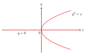
The first-order necessary condition for optimality of the lower level objective function with respect to is , which is equivalent to saying that or . Its graph is shown in Figure 2.
Since the objective of the lower level program is not convex in lower level variable , for each fixed , not all corresponding ’s lying on the curve are global optimal solutions of the lower level program. The true global optimal solutions for the lower level problem are shown in Figure 2. It is easy to see that
and is the unique global optimal solution.
Now we claim that the partial calmness for (CP) does not hold at . Indeed, the associated partially penalized problem is given by
| (3.3) |
Take any . For the objective values, we find
| (3.4) |
Thus, for holds, and this shows that is not a local minimizer of the associated partially penalized problem (3.3). Hence the partial calmness for (CP) does not hold at Moreover since (CP) is a standard nonlinear program, it is easy to check that the KKT condition does not hold at .
To explain our new approach, we now consider the following optimization problem in which we add the first and the second-order conditions to the value function reformulation of problem (3.1):
| (3.5) |
Since both the first and the second-order conditions for the lower level program hold at without any further assumption, the constraints and are redundant. Hence is still the optimal solution to the above problem.
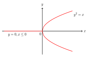
From the graph in Figure 2, we can see that any point satisfying the first and the second-order conditions together lies in the graph of the solution mapping . This means that the value function constraint can be removed and hence is a (local) minimizer of the following partially penalized problem with :
| (3.6) |
Problem (3.6) is a one-level optimization problem. Furthermore, it is easy to check that its KKT condition holds at .
Next we present a geometric explanation for Example 3.1.
For Example 3.1, the partial calmness for (CP) at means that for some , is still the optimal solution of the associated partially penalized problem (3.3), whose feasible set is given by Figure 2. But by (3.4), this is violated by taking points on the line in the feasible set.
To fix the above issue, we add the second-order necessary optimality condition of the lower level program in the combined problem (3.5). The advantage of using the second-order necessary optimality condition is that the feasible set of the new associated partially penalized problem (3.6) ruled out all of the points on the line which are actually local maxima for the lower level objective function with (see Figure 2).
4 Combined with second-order optimality conditions
A natural idea that comes from Example 3.1 is to add the second-order necessary optimality conditions of the lower level program in the combined problem. In this section, we consider combined problems with different kinds of second-order optimality conditions.
4.1 Unconstrained case
For the unconstrained bilevel programming problem
| (UBLPP) |
we propose the following combined program using the second-order necessary optimality condition:
| (CPSOC) | ||||
We denote the corresponding partially penalized problem for (CPSOC) (as in Definition 2.3) by (CPSOCμ). The problem (CPSOCμ) is a nonlinear semidefinite optimization problem. To derive an optimality condition for it, we may apply some constraint qualification, e.g., Robinson’s constraint qualification (or a generalized MFCQ) of nonlinear semidefinite optimization problems.
4.2 Constrained case
In the constrained case, as we reviewed in Section 2, there are four kinds of second-order optimality conditions: FJSOC, BSOC, SSOC, and WSOC.
4.2.1 Combined with the Fritz John second-order optimality condition
We say that is an FJSOC-point if for all , there exists such that
| (4.1) |
By Theorem 2.1, if then is an FJSOC-point for .
Now we define
and consider the following combined problem with FJSOC:
| (FJSOCP) |
Since it is not easy dealing with the set of indices of active inequalities in the critical cone, we propose to use the following set to relax the critical cone:
| (4.2) |
where is an FJ-multiplier. Under the strict complementarity, becomes in the above relationship. Hence implies that there are such that the following relaxed FJ system holds:
| (4.3) |
Denote by
| (4.4) |
where
| (4.5) |
Then problem (FJSOCP) can be reformulated as the following problem equivalently.
| (FJSOCP-2) | ||||
Problem (FJSOCP-2) can be considered as an optimization problem with implicit variables as studied in recent paper [8]. Since problem (FJSOCP-2) is still not practical to solve, we consider its explicit version—the relaxed combined problem with FJ second-order condition:
| (R-FJSOCP) | ||||
Recall that a set-valued map is inner semicompact at with respect to if for each sequence such that , there is a convergent sequence and a subsequence such that holds for all ; see e.g. [8, page 7]. Note that the mapping defined in (4.4) is automatically inner semicompact since the set of FJ multipliers are uniformly bounded, and the sequence in the definition can always be taken as zero. Hence by [8, Theorems 4.3 and 4.5] we have the following equivalence between the problem with implicit variables and its explicit form.
Proposition 4.5.
Let be a local (global) optimal solution to (BLPP). Then for each is a local (global) optimal solution of (R-FJSOCP). Conversely, let be a global optimal solution to (R-FJSOCP). Then is a global solution of (BLPP). Moreover if for each , is a local optimal solution to (R-FJSOCP), then is a local solution of (BLPP).
As in Definition 2.3, we can define partial calmness for (FJSOCP) and partial calmness for (R-FJSOCP), and denote the corresponding partially penalized problems by (FJSOCPμ) and (R-FJSOCPμ), respectively.
Different from the relation between the partial calmness condition for (CPFJ) and the partial calmness condition for (CPFJ) in [30, Theorem 4.4], the partial calmness condition for (FJSOCP) could not imply the partial calmness condition for (R-FJSOCP) directly because the critical cone has been relaxed in (R-FJSOCP). But as we will show in Proposition 4.6, the partial calmness condition for (CPFJ) implies the partial calmness condition for (R-FJSOCP). Note that this relation coincides with the result in Proposition 2.4. On the other hand, since , it is immediate that
| (4.6) |
where denotes the set of points which satisfy the Fritz John condition.
In the following proposition, we show that the partial calmness for (R-FJSOCP) at with is not stronger than the one for (CPFJ) at . Hence when the critical cone , one can always take a nonzero critical direction to obtain a combined program with weaker partial calmness condition.
Proposition 4.6.
Let be a local solution of (CPFJ). Suppose that the partial calmness condition for (CPFJ) holds at . Then, for each , is a local optimal solution of problem (R-FJSOCP) where the partial calmness condition holds. Conversely, suppose that problem (R-FJSOCP) is partially calm at a local solution and is a local solution of problem (CPFJ). Then problem (CPFJ) is partially calm at .
Proof.
Adding an additional variable and a superfluous constraint to problem (CPFJ), the first assertion follows from Proposition 2.4.
Now suppose that problem (R-FJSOCP) is partially calm at . Then there exist and a neighborhood of such that
where is the feasible region of problem (R-FJSOCPμ). Let be a feasible solution of problem (CPFJμ). Then is feasible to problem (R-FJSOCPμ). Hence it follows that the problem (CPFJ) is partially calm at . ∎
4.2.2 Combined with the basic second-order optimality condition
As reviewed in Section 2, under certain constraint qualifications, for and one of the second-order optimality conditions BSOC, WSOC, and SSOC holds. In this subsection, we study the combined problem with BSOC. We say that is a BSOC, WSOC, or SSOC point of respectively if Definition 2.2(i), 2.2(ii), or 2.2(iii) holds respectively. Now we define
It is easily seen that
| (4.7) |
Similar to the combined problem (FJSOCP), we consider the combined problem with basic (weak, strong) second-order optimality conditions (SOCP) where , respectively. Different from FJSOC, none of BSOC, WSOC, and SSOC is necessary without extra constraint qualifications. Thus this reformulation requires that BSOC, WSOC, and SSOC hold at the optimal solution of the lower level program. At least it requires that the KKT conditions hold at the optimal solutions of the lower level program (i.e., ).
Since it is difficult to express the set of indices of active inequalities directly in the combined problem (SOCP) with such that it is still an optimization problem with equality and inequality constraints, we relax the critical cone (2.1) as
| (4.8) | |||||
where is a KKT multiplier and (4.8) follows from
Hence we propose to consider the following relaxed problem for the combined problem (SOCP) with :
| (R-BSOCP) | ||||
Similar to Proposition 4.5, since there is the value function constraint, the combined problem (SOCP) and the relaxed combined problem (R-BSOCP) are both equivalent in global solutions to the original problem when the corresponding second-order optimality conditions hold [8, Theorem 4.3]. To state the relationship on local solutions, we define the following mapping:
| (4.9) |
where
| (4.10) |
Proposition 4.7.
Let be a local optimal solution to (BLPP). Suppose that the basic second-order optimality condition holds for the lower level problem at . Then for each is a local optimal solution of (R-BSOCP). Conversely, let be a local optimal solution to (R-BSOCP) for each , Furthermore, let be inner semicompact at with respect to . Then is a local solution of (BLPP).
Remark 4.2.
Next, we study the relation between the partial calmness for (R-BSOCP) and the partial calmness for (CP). Similar to Proposition 4.6, we can prove the following proposition.
Proposition 4.8.
Suppose that is a local solution of (R-BSOCP). Then the partial calmness for (R-BSOCP) holds at if and only if the partial calmness for (CP) holds at the local optimal solution . Furthermore, if holds at for the lower level problem , then for all , validity of the partial calmness condition for (CP) at the local optimal solution implies validity of the partial calmness condition for (R-BSOCP) at the local optimal solution .
4.2.3 Combined with the weak second-order optimality condition
If WSOC holds at the lower level, we can consider the following combined problem with WSOC:
| (WSOCP) | ||||
and propose the corresponding partial calmness condition. Here with means that
i.e., the matrix is a -copositive matrix.
But the copositive matrix condition in (WSOCP) is not easy to tackle because the critical subspace involves the set of indices of active inequalities of . To cope with this difficulty, the equivalence between the KKT points satisfying WSOC of the original problem and the reformulated problem by introducing the squared slack variables is very useful. Indeed, by Propositions 2.1 and 2.2, problem (WSOCP) is equivalent to the following reformulated problem by introducing the squared slack variables:
| (WSOCPZ) | ||||
Now it is worth noting that the critical subspace
does not involve the set of indices of active inequalities of .
4.2.4 Combined with the strong second-order optimality condition
If SSOC holds at the lower level for each , we can consider the following combined problem:
| (SSOCP) | ||||
Recall that for a closed convex cone , the class of all -copositive matrices is the dual cone of the convex hull of [19, Lemma 2.28]. This provides a natural generalization of the constraint in the unconstrained case. The problem (SSOCP) can be viewed as generalized semi-infinite programming problem [45, 49] or generalized copositive programming problem (set-semidefinite optimization) [10, 19]. Similarly as in section 4.2.3, to deal with the difficulty of the active index set, one can also use the squared-slack-variable trick here.
4.3 Examples and Summary
In this section, we have discussed different types of combined problems with second-order optimality conditions, called (FJSOCP), (SOCP), (SSOCP) and (WSOCP). To address the issue caused by the set of indices of active inequalities, we come up with the related relaxed problems, called (R-FJSOCP) and (R-BSOCP), and also the problem with squared slack variables (WSOCPZ). All of the combined and relaxed problems are equivalent to the original (BLPP) under some mild and necessary assumptions.
Similarly to [30, 51, 52], we have proposed various partial calmness conditions based on the combined problems above. We summarize the relationships between various partial calmness conditions in Figure 3.
Under the validity of the KKT condition, we can even establish the relationship between partial calmness for the FJ and the KKT type combined programs when the FJ multiplier considered satisfies . For example, even if the partial calmness for (CPFJ) holds for with , if the set of multiplier is not empty and , it can be shown that the partial calmness for (CP) holds for when is sufficiently large. This comes from the fact that , as .
Next, we use some nonconvex BLPPs to illustrate the combined approach with second-order optimality conditions and the necessary optimality conditions.
We first give an example for which the combined approach in [30, 52] fails, but the partial calmness and the necessary optimality condition will hold if one adds the basic second-order optimality condition for the lower level program in the associated combined problem.
Example 4.2.
| (4.11) | ||||
Claim: In this example, we will show that
-
•
the partial calmness for (CP) does not hold at ;
-
•
the partial calmness for (SOCP) with holds at ;
-
•
the partial calmness for (R-BSOCP) holds at for any ;
-
•
the partial calmness for (WSOCP) does not hold at ;
-
•
necessary optimality conditions fail to hold for (CP);
-
•
the S-stationarity condition holds for (R-BSOCP).
It is easy to see that
| (4.18) |
and is a global optimal solution. Moreover, .
Now we show that the partial calmness for (CP) does not hold at . Indeed, the associated partially penalized problem is given by
| (4.19) | ||||
Note that when , . For any fixed , the objective function value when Hence is not a local minimizer of the associated partially penalized problem (4.19) and the partial calmness for (CP) does not hold at .
Let us consider adding the second-order optimality conditions. The critical cone is given by
| (4.23) |
Since LICQ holds, coincides with and hence . Problem (SOCP) is given by
| (4.24) | ||||
Suppose . Then it must satisfy the KKT condition
with a unique multiplier . It follows that
| (4.25) |
But states that which is equivalent to saying that This means that the point with and does not satisfy and hence is not included in the set . By the expression for the solution set (4.18), we have . Hence the value function constraint in problem (4.24) holds for all . We therefore can remove the value function constraint from problem (4.24). This means that the partial calmness for (SOCP) with holds at with .
Now consider the (R-BSOCP):
| (4.26) | ||||
Let . Then for any sufficiently close to , condition is equivalent to . So similar to the analysis for the partial calmness for (SOCP) with , the value function constraint can be removed. Then the partial calmness for problem (R-BSOCP) holds at with .
Recall that and the partial calmness with the larger set would be harder to hold. By the expression for the critical cone in (4.23), we can obtain the expression for the critical subspace of the problem (4.11)
WSOC states that
Since when , is taken as zero, these points are still in the set and hence . Since , for this example, the partial calmness for (SOCP) with does not hold at and the partial calmness for (WSOCP) does not hold at .
In the following example, we show that the partial calmness for (WSOCP) may hold.
Example 4.3.
We compare the results for the two examples in the following table.
5 Conclusions
In this paper, we demonstrate that although the partial calmness condition is generic for a combined program with a first condition information, there are still cases where the partial calmness condition and the corresponding necessary optimality conditions do not hold. To deal with these cases, we propose to add both the first-order and the second-order optimality conditions of the lower level problem as constraints. There are several advantages in this approach. First, by adding extra constraints to the first-order combined problem, the new partial calmness condition and the resulting necessary optimality condition are easier to hold. Second, by adding second-order optimality conditions, it may be possible that the graph of the solution set to the lower level problem coincides with the set of second-order stationary points and hence the difficult value function constraint can be removed. However there are also some drawbacks to our second-order approach. First, by using a second-order optimality condition, we may need to introduce more extra variables other than the multipliers. Then similar to the difficulty in dealing with the reformulation involving with the KKT condition, the problem is no longer equivalent to the original bilevel program in the sense of local optimality. Second, since there are second-order optimality conditions in the feasible region of the partially penalized problem, constraint qualifications may be harder to verify for the partially penalized problem. Third, numerically the combined program with the second-order condition may sometimes be harder to solve than the combined program with the first-order condition. In our future work, we will try to utilize the advantages and address the drawbacks.
Acknowledgments
We thank the guest editor Tim Hoheisel and the two anonymous referees for their suggestions, which have helped to improve the presentation of this paper.
References
- [1] L. Adam, R. Henrion, and J.V. Outrata, On M-stationarity conditions in MPECs and the associated qualification conditions, Math. Program., 168 (2018), pp. 229-259.
- [2] G. Allende and G. Still, Solving bilevel programs with the KKT-approach, Math. Program., 138 (2013), pp. 309-332.
- [3] A.V. Arutyunov, Perturbations of extremum problems with constraints and necessary optimality conditions, J. Sov. Math., 54 (1991), pp. 1342-1400.
- [4] K. Bai and J.J. Ye, Directional necessary optimality conditions for bilevel programs, Math. Oper. Res., 47 (2022), pp. 1169-1191.
- [5] J. Bard, Practical Bilevel Optimization: Algorithms and Applications, Dordrecht: Kluwer Academic Publishers, 1998.
- [6] R. Behling, G. Haeser, A. Ramos, and D.S. Viana, On a conjecture in second-order optimality conditions, J. Optim. Theory Appl., 176 (2018), pp. 625-633.
- [7] M. Benko, H. Gfrerer, and J. V. Outrata, Calculus for directional limiting normal cones and subdifferentials, Set-Valued Var. Anal., 27 (2019), pp. 713-745.
- [8] M. Benko and P. Mehlitz, On implicit variables in optimization theory, J. Nonsmooth Anal. Optim., 2 (2021), doi:10.46298/jnsao-2021-7215.
- [9] J. F. Bonnans and A. Shapiro, Pertubation Analysis of Optimization Problems, Springer-Verlag, 2000.
- [10] S. Burer and H. Dong, Representing quadratically constrained quadratic programs as generalized copositive programs, Oper. Res. Lett., 40 (2012), pp. 203-206.
- [11] J.V. Burke, Calmness and exact penalization, SIAM J. Control Optim., 29 (1991), pp. 493-497.
- [12] F. H. Clarke, Optimization and Nonsmooth Analysis, Wiley-Interscience, New York, 1983.
- [13] S. Dempe, Foundations of Bilevel Programming, Kluwer Academic Publishers, Dordrecht, 2002.
- [14] S. Dempe and J. Dutta, Is bilevel programming a special case of a mathematical program with complementarity constraints?, Math. Program., 131 (2012), pp. 37-48.
- [15] S. Dempe, V. Kalashnikov, G. Prez-Valds, and N. Kalashnykova, Bilevel Programming Problems: Theory, Algorithms and Applications to Energy Systems, Springer, Berlin, 2015.
- [16] S. Dempe and A.B. Zemkoho, The bilevel programming problems: reformulations, constraint qualifications and optimality conditions, Math. Program., 138 (2013), pp. 447-473.
- [17] S. Dempe and A.B. Zemkoho, Bilevel Optimization: Advances and Next Challenges, Springer Optim. Appl, vol. 161, 2020.
- [18] C. Ding, D.F. Sun, and J.J. Ye, First order optimality conditions for mathematical programs with semidefinite cone complementarity constraints, Math. Program., 147 (2014), pp. 539-579.
- [19] G. Eichfelder and J. Jahn, Set-semidefinite optimization, J. Convex Anal., 15 (2008), pp. 767-801.
- [20] L. Franceschi, P. Frasconi, S. Salzo, R. Grazzi, and M. Pontil, Bilevel programming for hyperparameter optimization, ICML (2018), pp. 1563-1572.
- [21] E. H. Fukuda and M. Fukushima, A note on the squared slack variables technique for nonlinear optimization, J. Oper. Res. Soc. Jpn., 60 (2017), pp. 262-270.
- [22] J. Gauvin, A necessary and sufficient regularity condition to have bounded multipliers in nonconvex programming, Math. Program., 12 (1977), pp.136-138.
- [23] J. Gauvin and F. Dubeau, Differential properties of the marginal function in mathematical programming, Optimality and Stability in Mathematical Programming. Springer, Berlin, Heidelberg, 1982, pp. 101-119.
- [24] H. Gfrerer, On directional metric subregularity and second-order optimality conditions for a class of nonsmooth mathematical programs, SIAM J. Optim., 23 (2013), pp. 632-665.
- [25] H. Gfrerer and J.J. Ye, New constraint qualifications for mathematical programs with equilibrium constraints via variational analysis, SIAM J. Optim., 27 (2017), pp. 842-865.
- [26] H. Gfrerer and J.J. Ye, New sharp necessary optimality conditions for mathematical programs with equilibrium constraints, Set-Valued and Variational Analysis, 28 (2020), pp. 395-426.
- [27] H. Gfrerer, J.J. Ye, and J.C. Zhou, Second-order optimality conditions for non-convex set-constrained optimization problems, to appear in Math. Oper. Res., arXiv:1911.04076.
- [28] L. Guo, G.H. Lin, J.J. Ye, and J. Zhang, Sensitivity analysis of the value function for parametric mathematical programs with equilibrium constraints, SIAM J. Optim., 24 (2014), pp. 1206-1237.
- [29] R. Henrion and T.M. Surowiec, On calmness conditions in convex bilevel programming, Appl. Anal., 90 (2011), pp. 951-970.
- [30] R.Z. Ke, W. Yao, J.J. Ye, and J. Zhang, Generic property of the partial calmness condition for bilevel programming problems, SIAM J. Optim., 32 (2022), pp. 604-634.
- [31] G. Kunapuli, K. Bennett, J. Hu, and J.S. Pang, Classification model selection via bilevel programming, Optim. Meth. Softw., 23 (2008), pp. 475-489.
- [32] Y. C. Liang and J. J. Ye, Optimality conditions and exact penalty for mathematical programs with switching constraints, J. Optim. Theory Appl., 190 (2021), pp. 1-31.
- [33] R. Liu, P. Mu, X. Yuan, S.Z. Zeng, and J. Zhang, A generic first-order algorithmic framework for bi-level programming beyond lower-level singleton, ICML (2020), pp. 6305-6315.
- [34] P. Mehlitz, Stationarity conditions and constraint qualifications for mathematical programs with switching constraints, Math. Program., 181 (2020), pp. 149-186.
- [35] P. Mehlitz, On the linear independence constraint qualification in disjunctive programming, Optimization, 69 (2020), pp. 2241-2277.
- [36] P. Mehlitz and L.I. Minchenko, R-regularity of set-valued mappings under the relaxed constant positive linear dependence constraint qualification with applications to parametric and bilevel optimization, Set-Valued Anal., 30 (2022), pp. 179-205.
- [37] P. Mehlitz, L.I. Minchenko, and A.B. Zemkoho, A note on partial calmness for bilevel optimization problems with linearly structured lower level, Optim. Lett., 15 (2021), pp. 1277-1291.
- [38] L. Minchenko and A. Leschov, On strong and weak second-order necessary optimality conditions for nonlinear programming, Optimization, 65 (2016), pp. 1693-1702.
- [39] L. Minchenko and S. Stakhovski, Parametric nonlinear programming problems under the relaxed constant rank condition, SIAM J. Optim., 21 (2011), pp. 314-332.
- [40] J. Mirrlees, The theory of moral hazard and unobservable behaviour–part I, Rev. Econ. Stud., 66 (1999), pp. 3-22.
- [41] B.S. Mordukhovich, Variational Analysis and Applications, Springer, Cham, 2018.
- [42] B.S. Mordukhovich, N.M. Nam, and H.M. Phan, Variational analysis of marginal functions with applications to bilevel programming, J. Optim. Theory Appl., 152 (2012), pp. 557-586.
- [43] J.V. Outrata, On the numerical solution of a class of Stackelberg problems, ZOR-Math. Methods Oper. Res., 34 (1990), pp. 255-277.
- [44] K. Shimizu, Y. Ishizuka, and J. Bard, Nondifferentiable and Two-level Mathematical Programming, Kluwer Academic, 1997.
- [45] O. Stein, Bi-level strategies in semi-infinite programming, Springer Science and Business Media, 2013.
- [46] M.W. Xu and J.J. Ye, Relaxed constant positive linear dependence constraint qualification and its application to bilevel programs, J. Global Optim., 78 (2020), pp. 181-205.
- [47] J.J. Ye, Necessary optimality conditions for multiobjective bilevel programming problems, Math. Oper. Res., 36 (2011), pp. 165-184.
- [48] J.J. Ye, Constraint qualifications and optimality conditions in bilevel optimization, Bilevel Optimization: Advances and Next Challenges, ch. 8, Springer Optimization and its Applications vol. 161, 2020.
- [49] J.J. Ye and S.Y. Wu, First order optimality conditions for generalized semi-infinite programming problems. J. Optim. Theory Appl., 137 (2008), pp. 419-434.
- [50] J.J. Ye, X.M. Yuan, S.Z. Zeng, and J. Zhang, Difference of convex algorithms for bilevel programs with applications in hyperparameter selection, Math. Program., (2022) https://doi.org/10.1007/s10107-022-01888-3.
- [51] J.J. Ye and D.L. Zhu, Optimality conditions for bilevel programming problems, Optimization, 33 (1995), pp. 9-27.
- [52] J.J. Ye and D.L. Zhu, New necessary optimality conditions for bilevel programs by combining the MPEC and value function approaches, SIAM J. Optim., 20 (2010), pp. 1885-1905.