Bhatia-Davis formula in the quantum speed limit

Abstract

The Bhatia-Davis theorem provides a useful upper bound for the variance in mathematics, and in quantum mechanics, the variance of a Hamiltonian is naturally connected to the quantum speed limit due to the Mandelstam-Tamm bound. Inspired by this connection, we construct a formula, referred to as the Bhatia-Davis formula, for the characterization of the quantum speed limit in the Bloch representation. We first prove that the Bhatia-Davis formula is an upper bound for a recently proposed operational definition of the quantum speed limit, which means it can be used to reveal the closeness between the timescale of certain chosen states to the systematic minimum timescale. In the case of the largest target angle, the Bhatia-Davis formula is proved to be a valid lower bound for the evolution time to reach the target when the energy structure is symmetric. Regarding few-level systems, it is also proved to be a valid lower bound for any state in two-level systems with any target, and for most mixed states with large target angles in equally spaced three-level systems.

I Introduction

How fast a quantum system can evolve as required is usually referred to as the problem of quantum speed limit in quantum foundations. This problem is important in quantum foundations as it is naturally related to the uncertainty relations and other fundamental properties of quantum mechanics. For instance, the first bound concerning quantum speed limit given by Mandelstam and Tamm in 1945 Mandelstam1945 was derived based on the uncertainty relations. Nowadays, the quantum speed limit has gone way beyond the quantum foundations and attracted much attention from the community of quantum information and quantum technology due to the fact that the existence of noise is the major obstacle in most quantum information processing to provide true quantum advantages in practice, and fast evolutions could be a very useful approach to reduce the effect of noise in these processes and help to reveal the quantum advantage.

The historical development of quantum speed limit is basically the development of mathematical tools. Various tools have been developed for different scenarios Deffner2017 , including unitary dynamics Mandelstam1945 ; Margolus1998 ; Giovannetti2004 , open systems Taddei2013 ; Campo2013 ; Deffner2013 ; Sun2015 ; Marvian2015 ; Mirkin2016 ; Campo2019 ; Campaioli2018 ; Campaioli2019 ; Chenu17 ; Beau17b ; Cai2017 ; Villamizar2015 ; Sun2019 ; Meng2015 ; Mirkin2020 ; Zhang2014 ; Liu2015 ; Wu2018 ; Mondal2016 , quantum metrology Giovannetti2003 ; Giovannetti2006 ; Beau17a , quantum control Caneva2009 ; Hegerfeldt2013 ; Funo17 ; Campbell2017 ; Poggi2019 , quantum phase transitions Heyl2017 ; Shao2020 , quantum information processing Epstein2017 ; Girolami2019 ; Ashhab2012 , quantum resources Marvian2016 , geometry of quantum mechanics Pires2016 ; Bukov2019 ; Sun2021 , and even the classical systems Margolus11 ; Shanahan2018 ; Okuyama2018 ; Amari16 . The crossover between quantum speed limits has been observed in an optically trapped single atom system recently Ness2021 . Most existing tools in this field can be divided into the Mandelstam-Tamm type and Margolus-Levitin type, which originate from the Mandelstam-Tamm bound $\pi/(2\Delta H)$ Mandelstam1945 and the Margolus-Levitin bound $\pi/(2\langle H\rangle)$ Margolus1998 , where $\langle H\rangle$ is the expected value of the Hamiltonian $H$ and $\Delta H:=\sqrt{\langle H^{2}\rangle-\langle H\rangle^{2}}$ is the corresponding deviation. The major difference between these two types is that the former one is depicted by the deviation and the latter one uses only the expected value.

Different with these two types, an operational definition of quantum speed limit was proposed in 2020 Shao2020 based on the optimization of states that can fulfill the target. One advantage of this operational definition is its independence of the quantum states, which means it is the systematic minimum timescale for this target and determined only by the Hamiltonian structure. However, in quantum technology, some specific quantum states, like NOON states, cat states, or certain types of entangled states, may be more worth studying than a general one in some scenarios, and it is also possible that one does not care the systematic minimum timescale, but is more interested in the time scale of these specific states. In such cases, state-dependent tools could be more handy than the operational definition. In the meantime, since the operational definition includes only the information of systematic minimum timescale and corresponding optimal states, it cannot reflect the closeness of the timescales between concerned states and the optimal ones. Hence, the state-dependent tools, especially those can naturally connect to the operational definition, would be very helpful to reveal this closeness and thus more useful in practice. Searching such state-dependent tools is a major motivation of this paper.

In mathematics, for a set of bounded real numbers $\{x_{i}\}$ with the expected value $\bar{x}=\frac{1}{n}\sum_{i}x_{i}$ ($n$ is the number of elements), Bhatia and Davis provided a very useful upper bound on the variance $\mathrm{var}(x)=\frac{1}{n}\sum_{i}(x_{i}-\bar{x})^{2}$ in 2000 Bhatia2000 ,

$$\mathrm{var}(x)\leq(M-\bar{x})(\bar{x}-m),$$ (1)

where $m$, $M$ are the lower and upper bounds of the set, $m\leq x_{i}\leq M$ for any element $x_{i}$ in the set. This bound can be naturally extended to the statistics and further to the quantum mechanics. In quantum mechanics, the Bhatia-Davis inequality can be rewritten into $\Delta^{2}H\leq(E_{\max}-\langle H\rangle)(\langle H\rangle-E_{\min})$ with $E_{\max}$ and $E_{\min}$ the maximum and minimum energies with respect to $H$. Compared to the Mandelstam-Tamm bound, it is obvious that

$$\frac{\pi}{2\Delta H}\geq\frac{\pi}{2\sqrt{(E_{\max}-\langle H\rangle)(\langle H\rangle-E_{\min})}};$$ (2)

namely, the Bhatia-Davis inequality provides a lower bound for the Mandelstam-Tamm bound. Physically, the Bhatia-Davis bound indicates that the evolution time for a state to reach one of its orthogonal states is bounded by the gap between the maximum (minimum) energy and the average energy. However, since the Mandelstam-Tamm bound itself is attainable only for two-level pure states Deffner2017 ; Levitin2009 , the Bhatia-Davis bound above would be more difficult to saturate, and thus lack of practicability. Nevertheless, things are more complicated in the Bloch representation, which gives us a chance to introduce a similar formula by replacing $\pi$ to a general target angle $\Theta$ defined in the Bloch representation, and thoroughly study its role in quantum speed limit. In the entire paper this formula will be referred to as the Bhatia-Davis formula. The connection between this formula and the operational definition will be studied, along with its behaviors and roles in both multilevel and few-level systems from the aspect of quantum speed limit.

II Bhatia-Davis formula

II.1 Upper bound of the OQSL

The Bloch representation is a common geometric approach for quantum states, and widely applied in many topics in quantum information. In this representation, a $N$-dimensional density matrix $\rho$ can be expressed by

$$\rho=\frac{1}{N}\left(\openone+\sqrt{\frac{N(N-1)}{2}}\vec{r}\cdot\vec{\lambda}\right),$$ (3)

where $\vec{r}$ is a real vector referred to as the Bloch vector, $\openone$ is the identity matrix and $\vec{\lambda}$ is the $(N^{2}-1)$-dimensional vector of SU(N) generators. Throughout this paper, the target angle is defined by the angle between the Bloch vectors of the initial state $\vec{r}$ and its evolved state $\vec{r}(t)$ Campaioli2018 ; Campaioli2019 ; Shao2020

$$\theta(t,\vec{r})=\arccos\left(\frac{\vec{r}\cdot\vec{r}(t)}{|\vec{r}||\vec{r}(t)|}\right),$$ (4)

where $\theta(t,\vec{r})\in[0,\pi]$.

Inspired by the Bhatia-Davis inequality, we define the general form of Bhatia-Davis formula in the Bloch representation as

$$\tau_{\mathrm{BD}}:=\frac{\Theta}{2\sqrt{(E_{\mathrm{max}}-\langle H\rangle)(\langle H\rangle-E_{\min})}},$$ (5)

where $E_{\mathrm{max}}$ and $E_{\min}$ are the highest and lowest energies of the Hamiltonian $H$ and $\langle H\rangle=\mathrm{Tr}(\rho H)$ is the expected value with respect to the state $\rho$. $\Theta$ is a fixed target angle. In the entire paper, we denote $E_{k}$ ($|E_{k}\rangle$) as the $k$th eigenvalue (eigenstate) of $H$ with $k\in[0,N-1]$. Without loss of generality, we assume $E_{k}\leq E_{j}$ for $k<j$ and there exist at least two different energy values in $H$, namely, not all the equalities can be achieved simultaneously. Recently, Becker et al. Becker2021 provided a quantum speed limit, which also contains the maximum energy, with energy-constrained diamond norms between two unitaries. Traditionally, whether a bound contains the variance or the expected value is a major criterion to distinguish Mandelstam-Tamm type bounds and Margolus-Levitin type bounds. From this perspective, the Bhatia-Davis formula looks more like a Margolus-Levitin type as it contains the expected value. However, its dependence on the maximum and minimum energies makes it not a typical one. Hence, it may be more appropriate to be treated as a totally different type.

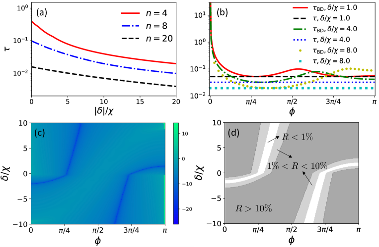
Figure 1: (a) The OQSL $\tau$ as a function of $|\delta|/\chi$ for particle number $n=4$ (solid red line), $n=8$ (dash-dotted blue line) and $n=20$ (dashed black line). (b) The Bhatia-Davis formula $\tau_{\mathrm{BD}}$ and the OQSL $\tau$ as a function of $\phi$ for different values of $\delta/\chi$. The solid red, dash-dotted green and circled yellow lines represent $\tau_{\mathrm{BD}}$ for $\delta/\chi=1.0,4.0,8.0$, and the dashed black, dotted blue and squared cyan lines represent $\tau$ for $\delta/\chi=1.0,4.0,8.0$, respectively. (c) The difference between $\tau_{\mathrm{BD}}$ and $\tau$ (in the scale of log) as a function of $\phi$ and $\delta/\chi$ for $n=10$. (d) The regimes in (c) that the relative difference $R=(\tau_{\mathrm{BD}}-\tau)/\tau<1\%$ (white area), $1\%<R<10\%$ (lightgray area) and $R>10\%$ (darkgray area). $\chi$ is set to be 1 in all panels.

Recently, an operational definition of the quantum speed limit (OQSL) was provided and discussed Shao2020 . The OQSL is defined via the set of states that can reach the target angle $\mathcal{S}:=\{\vec{r}|\theta(t,\vec{r})=\Theta,\exists t\}$. With this set, the OQSL (denoted by $\tau$) is defined as Shao2020

$$\tau = \min_{\vec{r}\in\mathcal{S}}t$$ (6)

$$\mathrm{subject}\leavevmode\nobreak\ \mathrm{to}\leavevmode\nobreak\ \leavevmode\nobreak\ \theta(t,\vec{r})=\Theta.$$

The Bhatia-Davis formula has a natural connection with the OQSL due to the following theorem.

Theorem 1.

For time-independent Hamiltonians under unitary evolution, the Bhatia-Davis formula is an upper bound for the OQSL:

$$\tau_{\mathrm{BD}}\geq\tau.$$ (7)

The proof is given in Appendix A. The equality can be attained when the average energy is half of the summation between the maximum and minimum energies. This theorem indicates that $\tau_{\mathrm{BD}}$ can reflect the closeness between the timescale of some specific states and the systematic minimum timescale when the equality is attainable.

In the following we take the generalized one-axis twisting model Kitagawa1993 ; Ma2011 ; Jin2009 as an example to discuss this theorem. The Hamiltonian for this model is

$$H=\chi J^{2}_{z}+\delta J_{z},$$ (8)

where $J_{z}=\sum^{n}_{i=1}\sigma^{(i)}_{z}/2$ with $\sigma^{(i)}_{z}$ the Pauli matrix along $z$-direction for the $i$th spin and $\chi$, $\delta$ are the coefficients. The Dicke state $|J=n/2,m\rangle$ ($m=0,\pm 1,\cdots,\pm J$ when $n$ is even and $m=\pm 1/2,\pm 3/2,\cdots,\pm J$ when $n$ is odd) is the eigenstate of $J_{z}$ with the corresponding eigenvalue $m$. For the sake of simplicity, here we assume $n$ is even and $\chi>0$. According to Ref. Shao2020 , the OQSL in this case can be expressed by $\tau=\Theta/(E_{\mathrm{max}}-E_{\min})$, where the maximum energy reads

$$E_{\max}=\frac{1}{4}\left(\chi n^{2}+2|\delta|n\right),$$ (9)

and the minimum energy reads

$$E_{\min}=\begin{cases}\chi\mathcal{R}^{2}(\frac{\delta}{2\chi})-\delta\mathcal{R}(\frac{\delta}{2\chi}),&\mathrm{for}\leavevmode\nobreak\ |\delta|/\chi\leq n,\\ \frac{1}{4}(\chi n^{2}-2|\delta|n),&\mathrm{for}\leavevmode\nobreak\ |\delta|/\chi>n.\end{cases}$$ (10)

Here $\mathcal{R}(\cdot)$ represents the function rounding to the nearest integer. The OQSL can then be obtained correspondingly. When $\delta=0$, the Hamiltonian is a standard one-axis twisting one, and the OQSL reduces to a simple form

$$\tau_{0}=\frac{4\Theta}{\chi n^{2}},$$ (11)

which decreases quadratically with the growth of particle number $n$. As a matter of fact, compared to $\tau_{0}$, the linear term $\delta J_{z}$ can facilitate the reduction of the OQSL, as shown in Fig. 1(a). For example, in the case of a small $\delta$, $\tau\propto 1/(\chi n^{2}+2|\delta|n)$. However, with the increase of $|\delta|$, when it is larger than $\chi n$, the OQSL becomes

$$\tau_{1}=\frac{\Theta}{|\delta|n},$$ (12)

which shows that the OQSL in this regime is not as sensitive as $\tau_{0}$ with respect to $n$.

In this model, a well-used state is the coherent spin state $\exp(\zeta J_{+}-\zeta^{*}J_{-})|J,J\rangle$ ($J_{\pm}=J_{x}\pm iJ_{y}$). Since $\zeta$ can be rewritten into $\zeta=-\frac{\phi}{2}\exp(-i\varphi)$ with $\phi\in[0,\pi]$ and $\varphi\in[0,2\pi]$, the coherent spin state can also be denoted by $|\phi,\varphi\rangle$. For this state, the Bhatia-Davis formula $\tau_{\mathrm{BD}}$ can be obtained by noticing the mean energy (details are given in Appendix A) is

$$\langle H\rangle=\frac{1}{4}\left(2\delta n\cos\phi+\chi n^{2}\cos^{2}\phi+\chi n\sin^{2}\phi\right),$$ (13)

which indicates $\tau_{\mathrm{BD}}$ is not affected by $\varphi$. Figure 1(b) shows the values of $\tau_{\mathrm{BD}}$ and $\tau$ as a function of $\phi$ for different values of $\delta$. In the case of $\delta=1.0$, two regimes of $\phi$ around $\pi/4$ and $3\pi/4$ are optimal for $\tau_{\mathrm{BD}}$ to attain $\tau$. However, with the increase of $\delta$ ($4.0$ and $8.0$ in the plot), the optimal regime around $\pi/4$ moves to the right and the optimal regime around $3\pi/4$ vanishes completely. To provide a complete picture of the attainable states, the difference between $\tau_{\mathrm{BD}}$ and $\tau$ (in the scale of log) is given in Fig. 1(c) as a function of $\phi$ and $\delta/\chi$, which confirms that the attainable regime for a large $\phi$ vanishes with the growth of $\delta$ when it is positive. As a matter of fact, most coherent spin states have chances to be the attainable states when $\delta$ is tuned to proper values. Particularly, the required optimal values of $\delta$ are very small when $\phi$ is less than $\pi/4$ or larger than $3\pi/4$. The states around $\phi=\pi/2$ are more difficult to be the attainable states since they require large values of $\delta$. However, although $\tau_{\mathrm{BD}}$ for these states are not optimal, when $\delta/\chi$ is larger than, for example around $10.0$, there is still a large regime around $\pi/2$ (on the left for $\delta/\chi>0$ and right for $\delta/\chi<0$) in which the relative difference $R=(\tau_{\mathrm{BD}}-\tau)/\tau$ is less than $10\%$, as shown in Fig. 1(d). In the meantime, the area in the plot for the regime that $R<1\%$ is around $7.9\%$ ($R<10\%$ is around $16.4\%$) of the total area, indicating that in this case, the timescale for the coherent spin states to reach the target could be very close to the systematic minimum time for a loose range of $\delta$. Another interesting phenomenon is that the behavior of the difference between $\tau_{\mathrm{BD}}$ and $\tau$ is dramatically different for positive and negative signs of $\delta/\chi$ when it is not very large. $\tau_{\mathrm{BD}}$ is way closer to $\tau$ for a negative (positive) $\delta/\chi$ when $\phi$ is small (large), which is due to the fact that $\langle H\rangle$ is closer to $(E_{\max}+E_{\min})/2$ for a negative (positive) value of $\delta/\chi$ when $\phi$ is small (large).

II.2 Largest target angle $\Theta=\pi$

In the study of quantum speed limit, the largest target angle $\Theta=\pi$ is worth paying particular attention as done in the Mandelstam-Tamm bound Mandelstam1945 and Margolus-Levitin bound Margolus1998 since it indicates the highest distinguishability. Due to the spirt of the operational definition, the set of states that can fulfill the target. i.e., the set $\mathcal{S}$, should be studied first as the state-dependent tools cannot reveal this information. Considering the unitary evolution, we have the following observations on the set $\mathcal{S}$ for the largest target $\Theta=\pi$.

Theorem 2.

For any finite-level Hamiltonian, there always exist states to fulfill the target $\Theta=\pi$, i.e., the set $\mathcal{S}$ cannot be an empty set. Furthermore, the set

$$\mathcal{S}_{0}\!:=\!\{\vec{r}\,|r^{2}_{j^{2}+2k-1}\!+\!r^{2}_{j^{2}+2k}\!=\!|\vec{r}|^{2},\forall j\!\in\![1,\!N\!-\!1],k\!\in\![0,j\!-\!1]\}$$

is always a subset of $\mathcal{S}$:

$$\mathcal{S}_{0}\subseteq\mathcal{S}.$$ (14)

Here $r_{i}$ is the $i$th entry of the Bloch vector $\vec{r}$. This theorem means that any state in $\mathcal{S}_{0}$ can fulfill the target regardless of the Hamiltonian structure. In the density matrix representation, the states in $\mathcal{S}_{0}$ take the form

$$\left(\begin{array}[]{cccccc}\frac{1}{N}&0&\cdots&\cdots&\cdots&0\\ 0&\frac{1}{N}&\vdots&\vdots&\vdots&\vdots\\ \vdots&\vdots&\ddots&\vdots&\rho_{kj}&\vdots\\ \vdots&\rho_{kj}^{*}&\vdots&\ddots&\vdots&\vdots\\ \vdots&\vdots&\vdots&\vdots&\frac{1}{N}&\vdots\\ 0&\cdots&\cdots&\cdots&\cdots&\frac{1}{N}\end{array}\right)$$ (15)

in the energy basis $\{|E_{k}\rangle\}$, where all the diagonal entries are $1/N$, and the only nonzero nondiagonal entries are the $kj$th and $jk$th ones with $j\in[1,N-1]$ and $k\in[0,j-1]$. Here $|\rho_{kj}|\in(0,1/N]$.

As a matter of fact, the theorem above also indicates that $\mathcal{S}_{0}$ is the minimum set for $\mathcal{S}$, which leads to an interesting question that what kind of Hamiltonians own the minimum set of $\mathcal{S}$? By denoting $\mathcal{E}_{\mathrm{d}}$ as the set of all the values of energy differences,

$$\mathcal{E}_{\mathrm{d}}=\{E_{j}-E_{k}|\forall j\in[1,N-1],k\in[0,j-1]\},$$ (16)

this question is answered by the corollary below.

Corollary 1.

For the target $\Theta=\pi$, if a Hamiltonian satisfies that the ratio between any two elements in $\mathcal{E}_{\mathrm{d}}$ cannot be written as the ratio between two odd numbers,

$$\frac{E_{j_{1}}-E_{k_{1}}}{E_{j_{2}}-E_{k_{2}}}\neq\frac{2m_{1}+1}{2m_{2}+1}$$ (17)

with $m_{1},m_{2}$ any two non-negative integers for any two different groups of subscripts $(j_{1},k_{1})$ and $(j_{2},k_{2})$, then

$$\mathcal{S}=\mathcal{S}_{0}.$$ (18)

Here two different groups of subscripts means that $j_{1}=j_{2}$ and $k_{1}=k_{2}$ cannot hold simultaneously. The proofs of the theorem and corollary above are given in Appendix B. A natural Hamiltonian structure to fit Eq. (17) is that all the elements in $\mathcal{E}_{\mathrm{d}}$ are noncommensurable to each other, which leads to the next corollary as follows.

Corollary 2.

For the target $\Theta=\pi$ and the Hamiltonians with noncommensurable energy differences, $\mathcal{S}=\mathcal{S}_{0}$.

Corollary 1 could lead to the following no-go corollary for multilevel systems (with at least three energy levels).

Corollary 3.

For multilevel systems with Hamiltonians stated in Corollary 1, no pure state can fulfill the target $\Theta=\pi$.

In practice, quantum systems are inevitably exposed to the environment and therefore suffer from the noises. Hence, the performance of $\mathcal{S}$ must be affected by the noise in general. The target $\Theta=\pi$ might be the most sensitive case as it requires a large rotation of the Bloch vector, which may not be possible in some type of noises. For example, if there exists a steady state for some noisy dynamics, it is very possible that the states, whose angle with the steady state are less than $\pi$, can never reach the target during the evolution for a large enough decay rate. Hence, the state number in the reachable state set $\mathcal{S}$ could be very limited, and even vanish in such cases. For the sake of a more intuitive understanding, here we take the damped five-level system as an example. The decoherence is described by the master equation Breuer2007

$$\partial_{t}\rho =-i[H,\rho]+\gamma_{0}(\bar{n}+1)\left(a\rho a^{\dagger}-\frac{1}{2}a^{\dagger}a\rho-\frac{1}{2}\rho a^{\dagger}a\right)$$

$$+\gamma_{0}\bar{n}\left(a^{\dagger}\rho a-\frac{1}{2}aa^{\dagger}\rho-\frac{1}{2}\rho aa^{\dagger}\right),$$ (19)

where $a$ ($a^{\dagger}$) is the lowering (raising) operator, $\gamma_{0}$ is a constant decay rate, and $\bar{n}=1/[e^{\omega_{0}/(k_{\mathrm{B}}T)}-1]$ is the Planck distribution with $k_{\mathrm{B}}$ the Boltzmann constant and $T$ the temperature. Now consider two groups of energies $\{E_{k}\}=\{1.0,2.1,4.5,8.3,11.0\}$ (denoted by $H_{1}$) and $\{E_{k}\}=\{1.0,2\sqrt{7},6\sqrt{2},6\sqrt{3},6\sqrt{5}\}$ (denoted by $H_{2}$). According to Corollaries 1 and 2, only the states in the form of Eq. (15), namely in the set $\mathcal{S}_{0}$, can reach the target $\Theta=\pi$ in the unitary dynamics. To show the influence of noise on $\mathcal{S}$, $5000$ random states in $\mathcal{S}_{0}$ are used to test the attainability of the target $\Theta=\pi$, as given in Fig. 2, for $H_{1}$ (red circles) and $H_{2}$ (blue squares). $\bar{n}$ is set to be 1 in the figure. In the absence of noise ($\gamma_{0}=0$), all states can reach the target, just as Theorem 2 stated. With the increase of decay rate, the number of states capable of reaching the target reduces in an approximately exponential way. When $\gamma_{0}=0.05$, a very limited number of states can still reach the target, and with the further increase of $\gamma_{0}$, no state can ever reach the target eventually.

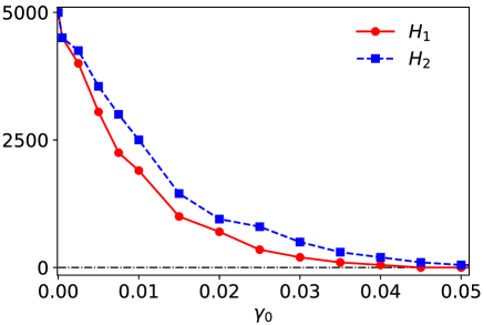
Figure 2: The variety of state number capable of reaching the target $\Theta=\pi$ with the change of decay rate $\gamma_{0}$ for the energy structures $\{1.0,2.1,4.5,8.3,11.0\}$ ($H_{1}$, red circles) and $\{1.0,2\sqrt{7},6\sqrt{2},6\sqrt{3},6\sqrt{5}\}$ ($H_{2}$, blue squares). $\bar{n}=1$ in the plot.

With the knowledge of $\mathcal{S}$, we could further study the Bhatia-Davis formula. In general, the Bhatia-Davis formula is not a valid lower bound for the evolution time to reach any target $\Theta$ due to Theorem 1. For those Hamiltonians that the equality in Theorem 1 is not attainable, $\tau_{\mathrm{BD}}$ is always larger than $\tau$. In this case, $\tau_{\mathrm{BD}}$ fails to be a valid lower bound for those states that reaches the OQSL, and hence not a lower bound in general. However, for the Hamiltonians and states that the equality can hold, $\tau_{\mathrm{BD}}$ might still be a valid lower bound. One useful scenario is demonstrated as follows.

Theorem 3.

For a finite-level Hamiltonian that the energies are symmetric about $\langle H\rangle$, the Bhatia-Davis formula is a valid lower bound for the evolution time to reach the target $\Theta=\pi$, and for the states in $\mathcal{S}$, it reduces to the OQSL.

The proof is given in Appendix B. For such a symmetric spaced energy structure, $\mathcal{S}$ must be larger than $\mathcal{S}_{0}$ since $E_{N-1-k}-E_{N-1-j}=E_{j}-E_{k}$ for any $k<j\leq\left\lfloor\frac{N-1}{2}\right\rfloor$ with $\lfloor\cdot\rfloor$ the floor function. In this case, apart from the states in Eq. (15), the states

$$\left(\begin{array}[]{ccccccc}\frac{1}{N}&0&\cdots&\cdots&\cdots&\cdots&0\\ 0&\frac{1}{N}&\vdots&\vdots&\vdots&\vdots&\vdots\\ \vdots&\vdots&\ddots&\rho_{kj}&\vdots&\vdots&\vdots\\ \vdots&\vdots&\rho^{*}_{kj}&\ddots&\rho_{N-1-j,N-1-k}&\vdots&\vdots\\ \vdots&\vdots&\vdots&\rho^{*}_{N-1-j,N-1-k}&\ddots&\vdots&\vdots\\ \vdots&\vdots&\vdots&\vdots&\vdots&\ddots&\vdots\\ 0&\cdots&\cdots&\cdots&\cdots&\cdots&\frac{1}{N}\end{array}\right)$$

are also always capable of reaching the target. An typical form of this symmetric structure is the equally spaced structure, i.e., $E_{k+1}-E_{k}$ is a constant for any legitimate $k$. Hence, one can immediately obtain the following corollary.

Corollary 4.

For an equally spaced finite-level Hamiltonian, the Bhatia-Davis formula is a valid lower bound for the evolution time to reach the target $\Theta=\pi$, and for the states in $\mathcal{S}$, it reduces to the OQSL.

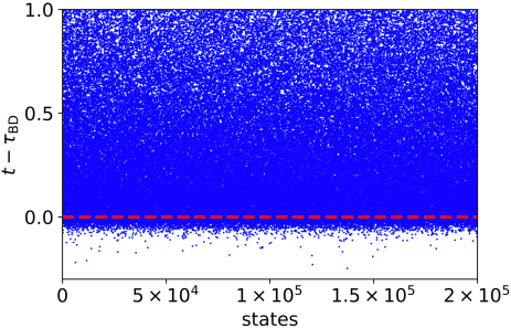
Figure 3: The difference between the evolution time to reach the target ($t$) and the Bhatia-Davis formula ($\tau_{\mathrm{BD}}$) for $2\times 10^{5}$ pairs of randomly generated five-level Hamiltonians and random states in $\mathcal{S}_{0}$.

Although the Bhatia-Davis formula is not a valid lower bound in general, how general it is still keeps undiscovered. For this sake, we numerically test whether $\tau_{\mathrm{BD}}$ is a valid lower bound for randomly generated five-level Hamiltonians and random initial states with the target $\Theta=\pi$. Since most randomly generated Hamiltonians satisfy the condition (17) in Corollary 1, most random initial states cannot fulfill the target expect for those in $\mathcal{S}_{0}$. This means $\tau_{\mathrm{BD}}$ is indeed a formal lower bound for these states as the true evolution time to reach the target is infinity. Hence, we pick only the random states in $\mathcal{S}_{0}$ for the test. Here $2\times 10^{5}$ random pairs of Hamiltonians and initial states in $\mathcal{S}_{0}$ are generated and tested, as shown in Fig. 3. It can be seen that even limited in the set $\mathcal{S}_{0}$, the difference between the evolution time $t$ (to reach the target) and $\tau_{\mathrm{BD}}$ is positive for most states (around $90\%$), and therefore $\tau_{\mathrm{BD}}$ is a valid lower bound for these $90\%$ states.

III Few-level systems

III.1 Two-level systems

The two-level system is the most well-studied model in the topic of quantum speed limit, and the only system that the well-known tools like the Mandelstam-Tamm bound Mandelstam1945 and the Margolus-Levitin bound Margolus1998 can be attained Deffner2017 ; Levitin2009 . In this system, denoting the ground and excited energies by $E_{0}$ and $E_{1}$ with the corresponding energy levels $|E_{0}\rangle$ and $|E_{1}\rangle$, we then have the following theorem.

Theorem 4.

For a two-level system under unitary evolution, the Bhatia-Davis formula is a valid lower bound for the evolution time to reach any target angle $\Theta$, and it can be attained by the states $(|E_{0}\rangle+e^{i\phi}|E_{1}\rangle)/\sqrt{2}$ with $\phi\in[0,2\pi)$.

The proof of this theorem is given in Appendix C. The attainability condition above comes from the requirement $\langle H\rangle=(E_{0}+E_{1})/2$. A corollary with respect to OQSL can be immediately obtained from this attainability condition.

Corollary 5.

For a two-level system under unitary evolution, the Bhatia-Davis formula (bound) reduces to OQSL when it is attainable.

With respect to the state-dependent bounds, several unified bounds have been developed. For example, Sun et al. Sun2021 provide an unified bound based on the changing rate of the phase in 2021. In the case of two-level systems, a well-known unified tool for quantum speed limit is Giovannetti2003 ; Giovannetti2004

$$\tau_{\mathrm{C}}=\max\left\{\frac{\mathcal{A}}{\Delta H},\frac{2\mathcal{A}^{2}}{\pi\langle H\rangle}\right\},$$ (20)

in which the target angle is defined via the Bures angle $\mathcal{A}=\arccos f$ with $f=\mathrm{Tr}\sqrt{\sqrt{\rho_{0}}\rho_{1}\sqrt{\rho_{0}}}$ the fidelity between two quantum states $\rho_{0}$ and $\rho_{1}$. In the meantime, another tool based on Bures angle is Taddei2013

$$\tau_{\mathrm{F}}=\frac{2\mathcal{A}}{\sqrt{F}},$$ (21)

with $F$ the quantum Fisher information with respect to the evolution time $t$. It is defined by $F=\mathrm{Tr}(\rho L^{2})$ with $L$ the symmetric logarithmic derivative. Here $L$ is determined by the equation $\partial_{t}\rho=(\rho L+L\rho)/2$. In the Bloch sphere ($|E_{1}\rangle$ as the north pole), the density matrix is $\rho=(\openone+\vec{r}\cdot\vec{\sigma})/2$ with $\sigma=(\sigma_{x},\sigma_{y},\sigma_{z})$ the vector of Pauli matrices. Then $\tau_{\mathrm{F}}$ can be expressed by

$$\tau_{\mathrm{F}}=\frac{2\mathcal{A}}{(E_{1}-E_{0})\sqrt{|\vec{r}|^{2}-r^{2}_{z}}},$$ (22)

which is larger than $2\mathcal{A}/\Delta H$ since here $\Delta H=(E_{1}-E_{0})\sqrt{1-r^{2}_{z}}/2$. They are equivalent when the initial state is pure. Combining several tools to construct a tighter bound for the quantum speed limit is a common method in the previous studies in this field. Using this strategy, the quantity

$$\tau_{\mathrm{m}}=\max\left\{\tau_{\mathrm{BD}},\tau_{\mathrm{F}},\frac{2\mathcal{A}^{2}(\Theta)}{\pi\langle H\rangle}\right\}$$ (23)

is a valid lower bound for the evolution time to reach the target in the case of two-level systems. Notice that $\tau_{\mathrm{BD}}$ is not be a valid lower bound in general for multilevel systems as discussed in the previous section, hence $\tau_{\mathrm{m}}$ cannot be directly extended to multilevel systems. Here $\mathcal{A}(\Theta)$ means the target is still defined via Eq. (4) and the value of $\mathcal{A}$ is calculated via $\Theta$ and the initial state. As a matter of fact, the fidelity between two qubits can be expressed by $f^{2}=\mathrm{Tr}(\rho_{0}\rho_{1})+2\sqrt{\det(\rho_{0})\det(\rho_{1})}$ with $\det(\cdot)$ the determinant Hubner1992 ; Hubner1993 . For unitary evolutions, it can be rewritten with the Bloch vectors into $f^{2}=1-\frac{1}{2}|\vec{r}|^{2}(1-\cos\theta)$, where $|\vec{r}|$ is the norm of the initial state. Hence, $\mathcal{A}(\Theta)=\arccos\sqrt{1-\frac{1}{2}|\vec{r}|^{2}(1-\cos\Theta)}$, which indicates $\mathcal{A}\leq\Theta/2$ and the equality holds for pure states. Because of this property, the following corollary holds.

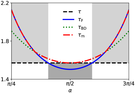
Figure 4: The behaviors of different tools as a function of $\alpha$. The dashed black, solid blue, dotted green and dash-dotted red lines represent the OQSL $\tau$, the bound based on quantum Fisher information $\tau_{\mathrm{F}}$, the Bhatia-Davis formula $\tau_{\mathrm{BD}}$, and the combined formula $\tau_{\mathrm{m}}$. The parameters are set as $E_{1}=2.0$, $E_{0}=1.0$, $|\vec{r}|=0.8$, and the target angle $\Theta=\pi/2$.

Corollary 6.

The Bhatia-Davis formula (bound) is equivalent to $\tau_{\mathrm{F}}$ for two-level pure states.

With this corollary, and noticing that $\tau_{\mathrm{F}}=\mathcal{A}/\Delta H$ for two-level pure states, it is easy to see that $\tau_{\mathrm{m}}$ reduces to $\tau_{\mathrm{C}}$ for two-level pure states. For mixed states, the relation between $\tau_{\mathrm{BD}}$, $\tau_{\mathrm{F}}$ and $2\mathcal{A}^{2}/(\pi\langle H\rangle)$ is undetermined. However, in many cases, for instance when $(E_{1}+E_{0})/(E_{1}-E_{0})>\sqrt{2}|\vec{r}|$ is satisfied, $\tau_{\mathrm{F}}$ is always larger than $2\mathcal{A}^{2}/(\pi\langle H\rangle)$, and the value of $\tau_{\mathrm{m}}$ is taken as the larger one between $\tau_{\mathrm{F}}$ and $\tau_{\mathrm{BD}}$. More calculation details can be found in Appendix C. An example is shown in Fig. 4 for the sake of a more intuitive understanding on $\tau_{\mathrm{m}}$. Here $\alpha$ is the angle between the Bloch vector $|\vec{r}|$ and $z$-axis. The states in the regime $\alpha\in[\Theta/2,\pi-\Theta/2]$ can fulfill the target Shao2020 . This plot first confirms that $\tau_{\mathrm{BD}}$ (dotted green line) is an upper bound for the OQSL $\tau$ (dashed black line). However, $\tau_{\mathrm{F}}$ (solid blue line) and $\tau_{\mathrm{BD}}$ do not have a fixed relation. $\tau_{\mathrm{F}}$ is less than $\tau_{\mathrm{BD}}$ for the states close to the $xy$ plane. Hence, $\tau_{\mathrm{m}}$ (dash-dotted red line) equals $\tau_{\mathrm{BD}}$ in this regime, and it is indeed the tightest bound for the evolution time. $2\mathcal{A}^{2}/(\pi\langle H\rangle)$ is not plotted due to the fact that it is significantly smaller than the others in this case.

Another advantage of using $\tau_{\mathrm{BD}}$ to construct the bound is that $\tau_{\mathrm{m}}$ is always larger than $\tau$ due to Theorem 1, and it reduces to $\tau$ in the $xy$ plane because of the attainability of $\tau_{\mathrm{BD}}$, which means $\tau_{\mathrm{m}}$ can reflect the fact that $\tau$ is the systematic minimum time to reach the target even when it is not attainable. In the meantime, $\tau_{\mathrm{F}}$ can show this capability only for some states (lightgray area), and it fails to do that for the states close to the $xy$ plane (darkgray area) as it is smaller than $\tau$ in this regime. Therefore, in the case where $\tau$ is not known, $\tau_{\mathrm{F}}$ cannot be used to estimate the true minimum timescale.

III.2 Three-level systems

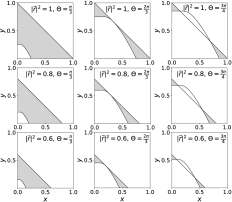
Figure 5: Regimes of $x$, $y$ (gray areas) in the reachable states set $\mathcal{S}$ for equally spaced three-level Hamiltonians with different values of $|\vec{r}|^{2}$ and $\Theta$. $x=r^{2}_{3}+r^{2}_{4}$ and $y=r^{2}_{0}+r^{2}_{1}+r^{2}_{5}+r^{2}_{6}$ in the plot.

Three-level systems are very common in the study of quantum optics and quantum information. As is the same as the general case, the Bhatia-Davis formula

$$\tau_{\mathrm{BD}}=\frac{\Theta}{2\sqrt{(E_{2}-\langle H\rangle)(\langle H\rangle-E_{0})}}$$ (24)

is not a valid lower bound in a general three-level system. However, Corollary 4 shows that $\tau_{\mathrm{BD}}$ is indeed a valid lower bound in the equally spaced three-level systems for $\Theta=\pi$. To find out if $\tau_{\mathrm{BD}}$ still remains a valid bound for a general target in this case, we need to study the set $\mathcal{S}$ first. Define $x=r^{2}_{3}+r^{2}_{4}$ and $y=r^{2}_{0}+r^{2}_{1}+r^{2}_{5}+r^{2}_{6}$ with $r_{i}$ ($i=0,\dots,6$) an entry of the Bloch vector, then for the states in $\mathcal{S}$, $x$ and $y$ must locate in the following two regimes

$$\begin{cases}y\geq 4|\vec{r}|\sin\left(\frac{\Theta}{2}\right)\sqrt{x}-4x,\\ y\leq 4x,\\ y\leq|\vec{r}|^{2}-x,\end{cases}$$ (25)

and

$$\begin{cases}y\geq 4|\vec{r}|\sin\left(\frac{\Theta}{2}\right)\sqrt{x}-4x,\\ y\geq 4x,\\ y\geq|\vec{r}|^{2}\sin^{2}\left(\frac{\Theta}{2}\right),\\ y\leq|\vec{r}|^{2}-x.\end{cases}$$ (26)

The thorough derivation is given in Appendix D. The full regime is illustrated in Fig. 5 (gray areas) for different values of $|\vec{r}|^{2}$ and $\Theta$. For the same $\Theta$ (columns in the plot), the shapes of the regime basically coincide for different values of $|\vec{r}|^{2}$, and its area shrinks with the reduction of $|\vec{r}|^{2}$. On the other hand, for the same $|\vec{r}|^{2}$ (rows in the plot), the regime becomes narrower when the value of $\Theta$ increases. These behaviors can also be reflected by the variety of the ranges of $x$ ($y$) along the $x$ axis ($y$ axis), which is in the regime $[|\vec{r}|^{2}\sin^{2}(\frac{\Theta}{2}),|\vec{r}|^{2}]$. The target $\Theta$ affects only the lower bound of this regime, which increases with the growth of $\Theta$. Hence, the area of the full regime becomes smaller when $\Theta$ gets larger. In the meantime, both bounds of this regime are affected by $|\vec{r}|^{2}$, and the largest range is attained at $|\vec{r}|^{2}=1$, indicating that there exist more choices of $x$, $y$ for pure states to reach the target.

Another interesting fact is that the full regime is continuous for the targets less than $2\pi/3$, and it splits into two areas for those larger than $2\pi/3$. This phenomenon is due to the fact that the minimum difference between $|\vec{r}|^{2}-x$ and $4|\vec{r}|\sin\left(\frac{\Theta}{2}\right)\sqrt{x}-4x$ with respect to $x$ is $|\vec{r}|^{2}\left[1-\frac{4}{3}\sin^{2}\left(\frac{\Theta}{2}\right)\right]$. When $\Theta\leq 2\pi/3$, this minimum value is always positive, indicating that all points on the line $y=4|\vec{r}|\sin\left(\frac{\Theta}{2}\right)\sqrt{x}-4x$ are feasible points in $\mathcal{S}$. By contrast, when $\Theta>2\pi/3$, only some points on this line are feasible, and the full regime then splits into two areas.

With the information of $\mathcal{S}$, we then provide the following theorem on the Bhatia-Davis formula.

Theorem 5.

For an equally spaced three-level system with a gap $\Delta$, the Bhatia-Davis formula is upper bounded by $\pi/(2\Delta)$,

$$\tau_{\mathrm{BD}}\leq\frac{\pi}{2\Delta},$$ (27)

for any $|\vec{r}|\in(0,1]$ and $\Theta\in(0,\pi]$.

The derivation is given in Appendix D. Since $\tau$ is upper bouned by $\tau_{\mathrm{BD}}$ according to Theorem 1, this result directly leads to $\tau\leq\pi/(2\Delta)$, which is fully reasonable as $\tau=\Theta/(2\Delta)$ in this case Shao2020 . Next we provide a theorem to show when $\tau_{\mathrm{BD}}$ is a valid lower bound for a general target.

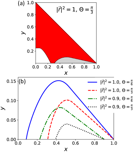
Figure 6: (a) Regimes of $x$, $y$ (red/dark gray areas in online/print version) that $\tau_{\mathrm{BD}}$ is always a valid lower bound in the case that $|\vec{r}|^{2}=1$ and $\Theta=\pi/3$. $x=r^{2}_{3}+r^{2}_{4}$ and $y=r^{2}_{0}+r^{2}_{1}+r^{2}_{5}+r^{2}_{6}$ in the plot. (b) The variety of borderline given in Eq. (32) as a function of $|\vec{r}|^{2}$ and $\Theta$.

Theorem 6.

For an equally spaced three-level system with the gap $\Delta$, the Bhatia-Davis formula is a valid lower bound for the evolution time to reach any target $\Theta\in(0,\pi]$ at least for the states in the regimes

$$\begin{cases}y\geq 4|\vec{r}|\sin\left(\frac{\Theta}{2}\right)\sqrt{x}-4x,\\ y\geq 4x,\\ y\geq|\vec{r}|^{2}\sin^{2}\left(\frac{\Theta}{2}\right),\\ y\leq|\vec{r}|^{2}-x,\end{cases}$$ (28)

and

$$\begin{cases}y\geq 4|\vec{r}|\sin\left(\frac{\Theta}{2}\right)\sqrt{x}-4x,\\ y\leq 4x,\\ y\leq|\vec{r}|^{2}-x,\\ y\sin^{2}(\frac{\Delta\tau_{\mathrm{a}}}{2})\leq|\vec{r}|^{2}\sin^{2}\!(\frac{\Theta}{2})-x\sin^{2}(\Delta\tau_{\mathrm{a}}).\end{cases}$$ (29)

In this theorem, $\tau_{\mathrm{a}}$ is defined by

$$\tau_{\mathrm{a}}:=\frac{\Theta}{2\Delta\sqrt{1-\frac{4}{3}(|\vec{r}|^{2}-x-y)}}$$ (30)

for $x+y\geq|\vec{r}|^{2}-1/3$ and

$$\tau_{\mathrm{a}}:=\frac{\Theta}{2\Delta\sqrt{1\!-\!\left[\frac{1}{2}+\sqrt{\frac{1}{3}(|\vec{r}|^{2}\!-\!x\!-\!y\!-\!\frac{1}{4})}\right]^{2}}}$$ (31)

for $x+y\leq|\vec{r}|^{2}-1/3$. The regime of the states given in the above theorem is illustrated in the case of $|\vec{r}|^{2}=1$ and $\Theta=\pi/3$ [red (dark gray) area in Fig. 6(a)]. For the states not in this regime (in the gray area), there exist states for which the Bhatia-Davis formula fails to be a valid lower bound. An interesting fact is that $\tau_{\mathrm{BD}}$ is a valid lower bound for most edges, for example, (1) $x=0$ and $y\neq 0$, i.e., nondiagonal states with $\rho_{12}=0$; (2) $x+y=|\vec{r}|^{2}$, which means $r_{2}=r_{7}=0$, i.e., states with all diagonal entries $1/3$. The borderline between the red (dark gray) and gray regimes reads

$$x\sin^{2}(\Delta\tau_{\mathrm{a}})+y\sin^{2}\left(\frac{\Delta\tau_{\mathrm{a}}}{2}\right)=|\vec{r}|^{2}\sin^{2}\left(\frac{\Theta}{2}\right).$$ (32)

As shown in Fig. 6(b), the area of violation regime (inside the line) grows with the increase of $|\vec{r}|^{2}$ or the decrease of $\Theta$, indicating that $\tau_{\mathrm{BD}}$ is a valid lower bound for most mixed states, especially when $\Theta$ is large. As a matter of fact, apart from the case $|\vec{r}|^{2}=1,\Theta=\pi/3$, this regime is very insignificant for other examples given in Fig. 5. Hence, in equally spaced three-level systems, $\tau_{\mathrm{BD}}$ is indeed a valid lower bound for most states, especially mixed states with large target angles.

IV conclusion

Inspired by the Bhatia-Davis theorem in mathematics and statistics, in this paper we construct a formula, referred to as the Bhatia-Davis formula, for the characterization of quantum speed limit in the Bloch representation. In a general multilevel system, we first prove that the Bhatia-Davis formula is an upper bound for the operational definition of quantum speed limit, and it reduces to the operational definition when the average energy is half of the summation between the maximum and minimum energies. The behaviors of both the operational definition and Bhatia-Davis formula are discussed in the generalized one-axis twisting model as an example. In the case of largest target angle, the reachable state set $\mathcal{S}$ are first studied and the Bhatia-Davis formula is then proved to be a valid lower bound for the evolution time to reach the target in systems with symmetric energy structures.

With respect to few-level scenarios, the two-level systems are first studied, and the Bhatia-Davis formula is proved to be a valid lower bound in this case, and it reduces to the operational definition when attainable. Another alternative state-dependent bound is also constructed using the Bhatia-Davis formula, which is tighter than the bound given by the quantum Fisher information. In the case of equally spaced three-level systems, the regime that the Bhatia-Davis formula remains a valid lower bound is given. Even though it is not in general, the violation becomes very insignificant for mixed states, especially when the target angle is large. Therefore, it could be approximately treated as a valid lower bound for most mixed states with large target angles in this type of systems.

Appendix A Calculation details for Theorem 1 and its applications

We first introduce the notation again for a better reading experience of the appendix. $E_{i}$ is the $i$th energy of the Hamiltonian $H$ with the corresponding eigenstate $|E_{i}\rangle$. Without loss of generality, here we assume $E_{0}\leq E_{1}\leq\cdots\leq E_{N-1}$ with $N$ the dimension of $H$. In the energy basis $\{|E_{i}\rangle\}$, a density matrix can be expressed by $\rho=\sum_{ij}\rho_{ij}|E_{i}\rangle\langle E_{j}|$, which immediately gives $\langle H\rangle=\sum_{i}\rho_{ii}E_{i}$. Now define a function

$$f(x):=\sum_{i}\rho_{ii}(E_{i}-x)^{2}.$$ (33)

It is easy to see that $x=\sum_{i}\rho_{ii}E_{i}=\langle H\rangle$ is the minimum value of this function by calculating the first and second derivatives. Therefore, one can obtain

$$f\left(\frac{E_{0}+E_{N-1}}{2}\right)\geq f(\langle H\rangle).$$ (34)

Next, by noticing that

$$f\left(\frac{E_{0}+E_{N-1}}{2}\right)-f(\langle H\rangle)$$ (35)

$$= \frac{1}{4}(E_{N-1}-E_{0})^{2}\!-\!(E_{N-1}-\langle H\rangle)(\langle H\rangle-E_{0}),$$

one can obtain

$$\frac{1}{4}(E_{N-1}-E_{0})^{2}\geq(E_{N-1}-\langle H\rangle)(\langle H\rangle-E_{0}),$$ (36)

which leads to the result of our theorem below

$$\frac{\Theta}{2\sqrt{(E_{N-1}-\langle H\rangle)(\langle H\rangle-E_{0})}}\geq\frac{\Theta}{E_{N-1}-E_{0}},$$ (37)

where $\Theta$ is the target angle and $\Theta/(E_{N-1}-E_{0})$ is the OQSL for time-independent Hamiltonians Shao2020 . Theorem 1 is then proved. $\blacksquare$

Now consider the generalized one-axis twisting Hamiltonian

$$H=\delta J_{z}+\chi J^{2}_{z},$$ (38)

where the angular momentum $J_{z}=\sum^{n}_{i=1}\sigma^{(i)}_{z}/2$ with $\sigma^{(i)}_{z}$ the Pauli matrix along the $z$-axis for $i$th spin. The coherent spin state can be expressed by

$$|\psi\rangle=e^{\zeta J_{+}-\zeta^{*}J_{-}}|J,J\rangle,$$ (39)

where $J_{\pm}=J_{x}\pm iJ_{y}$. Since $[J_{\pm},J_{z}]=\mp J_{\pm}$ and $[J_{+},J_{-}]=2J_{z}$, one can obtain

$$e^{-(\zeta J_{+}-\zeta^{*}J_{-})}J_{z}e^{\zeta J_{+}-\zeta^{*}J_{-}}$$ (40)

$$= \cos(2|\zeta|)J_{z}+\frac{\sin(2|\zeta|)}{2|\zeta|}(\zeta J_{+}+\zeta^{*}J_{-}),$$

which immediately gives $\langle\psi|J_{z}|\psi\rangle=J\cos(2|\zeta|)$ and

$$\langle\psi|J^{2}_{z}|\psi\rangle=J^{2}\cos^{2}(2|\zeta|)+\frac{1}{2}J\sin^{2}(2|\zeta|).$$ (41)

Hence, the expected value is

$$\langle H\rangle=\delta J\cos(2|\zeta|)+\chi J^{2}\cos^{2}(2|\zeta|)+\frac{\chi}{2}J\sin^{2}(2|\zeta|).$$

Due to the fact that $|\zeta|=\phi/2$ and $J=n/2$, the equation above can be rewritten as

$$\langle H\rangle=\frac{1}{4}\left(2\delta n\cos\phi+\chi n^{2}\cos^{2}\phi+\chi n\sin^{2}\phi\right).$$ (42)

Appendix B Calculations and proofs in the case of largest target angle

For the time-independent Hamiltonians under unitary evolution, the set $\mathcal{S}$ in the energy basis $\{|E_{k}\rangle\}$ can be written as Shao2020

$$\mathcal{S} = \Bigg{\{}\vec{r}\leavevmode\nobreak\ \Big{|}1-\cos\Theta=\frac{1}{|\vec{r}|^{2}}\sum^{N-1}_{j=1}\sum^{j-1}_{k=0}\left\{1-\cos\left[(E_{j}-E_{k})t\right]\right\}$$ (43)

$$\times\left(r^{2}_{j^{2}+2k-1}+r^{2}_{j^{2}+2k}\right),\exists t\Bigg{\}},$$

where $N$ is the dimension of Hamiltonian, $r_{i}$ is the $i$th entry of the Bloch vector. Here the SU($N$) generators $\{\lambda_{i}\}$ are generated via the rules

$$\mathrm{(1)}\leavevmode\nobreak\ \lambda_{l^{2}-2}=\sqrt{\frac{2}{l(l-1)}}\mathrm{diag}(1,1,\dots,1-l,0,\dots)$$ (44)

for $l=2,3,\dots,N$, namely, the first $l-1$ diagonal entries are 1, the $l$th entry is $1-l$, and zero for others. (2) For $j\in[1,N-1]$ and $k\in(0,j-1]$, the only nonzero entries in $\lambda_{j^{2}+2k-1}$ are the $kj$th and $jk$th ones, and the corresponding values are 1. (3) For $j\in[1,N-1]$ and $k\in(0,j-1]$, the only nonzero entries in $\lambda_{j^{2}+2k}$ are the $kj$th and $jk$th ones, and the corresponding values are $-i$ and $i$, respectively. Specifically, in the basis $\{E_{k}\}$ they can be expressed by

$$\lambda_{j^{2}+2k-1}=\left(\begin{array}[]{cccccc}0&\cdots&\cdots&\cdots&\cdots&0\\ 0&0&\vdots&\vdots&\vdots&\vdots\\ \vdots&\cdots&\ddots&\cdots&1&\vdots\\ \vdots&1&\cdots&\ddots&\cdots&\vdots\\ \vdots&\vdots&\vdots&\vdots&0&\vdots\\ 0&\cdots&\cdots&\cdots&\cdots&0\end{array}\right),$$ (45)

and

$$\lambda_{j^{2}+2k}=\left(\begin{array}[]{cccccc}0&\cdots&\cdots&\cdots&\cdots&0\\ 0&0&\vdots&\vdots&\vdots&\vdots\\ \vdots&\cdots&\ddots&\cdots&-i&\vdots\\ \vdots&i&\cdots&\ddots&\cdots&\vdots\\ \vdots&\vdots&\vdots&\vdots&0&\vdots\\ 0&\cdots&\cdots&\cdots&\cdots&0\end{array}\right).$$ (46)

In the case that the target $\Theta=\pi$, the constraint on $t$ in the equation above reduces to

$$2=\sum^{N-1}_{j=1}\sum^{j-1}_{k=0}\left\{1-\cos\left[(E_{j}-E_{k})t\right]\right\}\frac{r^{2}_{j^{2}+2k-1}+r^{2}_{j^{2}+2k}}{|\vec{r}|^{2}}.$$ (47)

Since $1-\cos\left[(E_{j}-E_{k})t\right]\leq 2$ and

$$\frac{1}{|\vec{r}|^{2}}\sum^{N-1}_{j=1}\sum^{j-1}_{k=0}r^{2}_{j^{2}+2k-1}+r^{2}_{j^{2}+2k}\leq 1,$$ (48)

the only solutions for Eq. (47) are

$$(E_{j}-E_{k})t=(2m+1)\pi,\leavevmode\nobreak\ \leavevmode\nobreak\ m=0,1,2,\cdots$$ (49)

for all pairs of $j$ and $k$ that satisfy $r^{2}_{j^{2}+2k-1}+r^{2}_{j^{2}+2k}\neq 0$. In the meantime, these solutions are valid only when the equality in inequality (48) are attained, which also requires the following additional condition:

$$r_{l^{2}-2}=0,\forall l=2,3,\cdots,N.$$ (50)

A useful fact is that in this case, regardless of the energy structures, the state satisfying

$$r^{2}_{j^{2}+2k-1}+r^{2}_{j^{2}+2k}=|\vec{r}|^{2}$$ (51)

for $j\in[1,N-1]$ and $k\in[0,j-1]$ can always reach the target $\Theta=\pi$ at the time

$$t=\frac{\pi}{E_{j}-E_{k}}.$$ (52)

Hence, $\mathcal{S}$ is not an empty set here, and in the meantime, the set

$$\mathcal{S}_{0}\!=\!\{\vec{r}\,|r^{2}_{j^{2}+2k-1}\!+\!r^{2}_{j^{2}+2k}\!=\!|\vec{r}|^{2},\forall j\!\in\![1,N\!-\!1],k\!\in\![0,j\!-\!1]\}$$ (53)

is always a subset of $\mathcal{S}$. Theorem 2 is then proved. $\blacksquare$

In fact, since $\lambda_{l^{2}-2}$ ($l=2,3,\dots,N$) is a diagonal SU($N$) generator, Eq. (50) indicates that in the energy basis, the diagonal entries of the density matrices which leads to valid solutions of $t$ must be $1/N$. In the case of $N>2$ it cannot be pure states. Corollary 3 is then prove. $\blacksquare$

One should notice that whether Eq. (49) has more solutions apart from Eq. (52) depends on the energy structure. Recall that we assume $E_{0}\leq E_{1}\leq\cdots\leq E_{N-1}$ and there exist at least two different energies. Now denote $\mathcal{E}_{\mathrm{d}}$ as the set of all energy differences:

$$\mathcal{E}_{\mathrm{d}}=\{E_{j}-E_{k}|\,\forall j\in[1,N-1],k\in[0,j-1]\}.$$ (54)

If the ratio between any two elements in $\mathcal{E}_{\mathrm{d}}$ cannot be written in the form of $(2m_{1}+1)/(2m_{2}+1)$ with $m_{1}$, $m_{2}$ any two non-negative integers, then only one pair of $(j,k)$ is allowed to satisfy $r^{2}_{j^{2}+2k-1}+r^{2}_{j^{2}+2k}\neq 0$ to make sure Eq. (49) has solutions, which means there are no other solutions except for Eq. (52), namely, $\mathcal{S}=\mathcal{S}_{0}$. One interesting specific example here is that all the elements in $\mathcal{E}_{\mathrm{d}}$ are noncommensurable to each other, which naturally fit the case that any two elements cannot be written in the form of $(2m_{1}+1)/(2m_{2}+1)$.

Furthermore, due to the expressions of $\lambda_{j^{2}+2k-1}$ and $\lambda_{j^{2}+2k}$ given in Eqs. (45) and (46), in the density matrix representation, the states in $\mathcal{S}_{0}$ must take the form

$$\left(\begin{array}[]{cccccc}\frac{1}{N}&\cdots&\cdots&\cdots&\cdots&0\\ \vdots&\frac{1}{N}&\vdots&\vdots&\vdots&\vdots\\ \vdots&\vdots&\ddots&\vdots&\rho_{kj}&\vdots\\ \vdots&\rho_{kj}^{*}&\vdots&\ddots&\vdots&\vdots\\ \vdots&\vdots&\vdots&\vdots&\frac{1}{N}&\vdots\\ 0&\cdots&\cdots&\cdots&\cdots&\frac{1}{N}\end{array}\right),$$ (55)

where all the diagonal entries are $1/N$, and all the nondiagonal entries are zero except for the $kj$th and $jk$th ones. Corollaries 1 and 2 are then proved. $\blacksquare$

In the following we continue to prove Theorem 3. Since the generators $\lambda_{l^{2}-2}$ for $l=2,3,\cdots,N$ are diagonal, Eq. (50) indicates that

$$\vec{r}\cdot\mathrm{Tr}(H\vec{\lambda})=\sum_{jk}r_{j}E_{k}\langle E_{k}|\lambda_{j}|E_{k}\rangle=0.$$ (56)

This is due to the fact that for those nonzero entries of $\vec{r}$, the corresponding SU($N$) generators have no nonzero diagonal entries. Therefore, the average energy reads

$$\langle H\rangle=\frac{1}{N}\mathrm{Tr}(H)=\frac{1}{N}\sum^{N-1}_{k=0}E_{k}.$$ (57)

In the case that the energies are symmetric about $(E_{0}+E_{N-1})/2$,

$$E_{N-1}+E_{0}=E_{N-1-k}+E_{k}$$ (58)

for any subscript $k$ satisfying $E_{k}\leq(E_{0}+E_{N-1})/2$, the average energy further reduces to

$$\langle H\rangle=\frac{1}{2}(E_{0}+E_{N-1}),$$ (59)

and the Bhatia-Davis formula reduces to

$$\tau_{\mathrm{BD}}=\frac{\pi}{E_{N-1}-E_{0}},$$ (60)

which is nothing but the OQSL Shao2020 . Hence, $\tau_{\mathrm{BD}}$ is a valid lower bound in this case. For the states not in $\mathcal{S}$, the target cannot be fulfilled, meaning that the time is infinite, and $\tau_{\mathrm{BD}}$ is also a valid formal lower bound. Thus, for a symmetric spaced Hamiltonian, $\tau_{\mathrm{BD}}$ is a valid state-dependent lower bound for $\Theta=\pi$. Theorem 3 is then proved. $\blacksquare$

Moreover, Eq. (58) indicates that

$$\frac{E_{N-1-k}-E_{N-1-m}}{E_{m}-E_{k}}=1$$ (61)

for $k<j\leq\lfloor\frac{N-1}{2}\rfloor$ with $\lfloor\cdot\rfloor$ the floor function, which means Eq. (49) for the pairs of subscripts $j,k$ and $N-1-k,N-1-j$ can always hold simultaneously. Hence, the states satisfying

$$|\vec{r}|^{2} = r^{2}_{j^{2}+2k-1}+r^{2}_{j^{2}+2k}+r^{2}_{(N-1-k)^{2}+2(N-1-j)-1}$$ (62)

$$+r^{2}_{(N-1-k)^{2}+2(N-1-j)}$$

can always fulfill the target $\Theta=\pi$ in this case. In the density matrix representation, due to Eqs. (45) and (46), these state are of the form

$$\left(\begin{array}[]{ccccccc}\frac{1}{N}&0&\cdots&\cdots&\cdots&\cdots&0\\ 0&\frac{1}{N}&\vdots&\vdots&\vdots&\vdots&\vdots\\ \vdots&\vdots&\ddots&\rho_{kj}&\vdots&\vdots&\vdots\\ \vdots&\vdots&\rho^{*}_{kj}&\ddots&\rho_{N-1-j,N-1-k}&\vdots&\vdots\\ \vdots&\vdots&\vdots&\rho^{*}_{N-1-j,N-1-k}&\ddots&\vdots&\vdots\\ \vdots&\vdots&\vdots&\vdots&\vdots&\ddots&\vdots\\ 0&\cdots&\cdots&\cdots&\cdots&\cdots&\frac{1}{N}\end{array}\right).$$

Appendix C Calculation details in two-level systems

Now we prove that the Bhatia-Davis formula is a valid lower bound in two-level systems under unitary evolution. For a two-level system, the Bloch vector of a state can be expressed by

$$\vec{r}=\eta(\sin\alpha\cos\varphi,\sin\alpha\sin\varphi,\cos\alpha)^{\mathrm{T}},$$ (63)

where $\eta\in(0,1]$, $\alpha\in[0,\pi]$, $\varphi\in[0,2\pi]$ and the superscript T represents the transposition. In this case, the set $\mathcal{S}$ reads Shao2020

$$\mathcal{S}=\left\{\vec{r}\leavevmode\nobreak\ \Big{|}\eta\in(0,1],\alpha\in\left[\frac{\Theta}{2},\pi-\frac{\Theta}{2}\right]\!,\varphi\in[0,2\pi]\right\}\!.$$ (64)

From the analysis in Appendix D of Ref. Shao2020 , one can see that for $\alpha\leq\pi/2$, the evolution time for the states in $\mathcal{S}$ to reach the target angle $\Theta$ can be expressed by

$$t=\frac{2}{E_{1}-E_{0}}\arcsin\left(\frac{\sin(\frac{\Theta}{2})}{\sin\alpha}\right),$$ (65)

for $\alpha>\Theta/2$, and $t=\pi/(E_{1}-E_{0})$ for $\alpha=\Theta/2$. Furthermore, $\tau_{\mathrm{BD}}$ in this case can be calculated as

$$\tau_{\mathrm{BD}}=\frac{\Theta}{(E_{1}-E_{0})\sqrt{1-\eta^{2}\cos^{2}\alpha}},$$ (66)

from which one can see that $\tau_{\mathrm{BD}}$ is a monotonically increasing function with respect to $|\vec{r}|$:

$$\tau_{\mathrm{BD}}\leq\frac{\Theta}{(E_{1}-E_{0})\sin{\alpha}}.$$ (67)

From the trigonometric inequality $\sin x\leq x$, it is easy to see $x\leq\arcsin x$. Utilizing this inequality, we have

$$\frac{\sin\left(\frac{\Theta}{2}\right)}{\sin\alpha}\leq\arcsin\left(\frac{\sin(\frac{\Theta}{2})}{\sin\alpha}\right),$$ (68)

which immediately gives

$$t\geq\frac{\Theta}{(E_{1}-E_{0})\sin{\alpha}}\geq\tau_{\mathrm{BD}}.$$ (69)

Furthermore, one should notice that $\tau_{\mathrm{BD}}$ can be attained when $\alpha=\pi/2$. The case of $\alpha>\pi/2$ can be analyzed similarly due to the symmetry of the dynamics. For the states out of $\mathcal{S}$, the target angle cannot be reached, indicating that any finite value could be a mathematically valid lower bound for it. Therefore, $\tau_{\mathrm{BD}}$ is also a valid bound in this regime. Theorem 4 is then proved. $\blacksquare$

Recall that $\tau_{\mathrm{F}}=2\mathcal{A}/\sqrt{F}$ and $\tau_{\mathrm{C}}=\max\left\{\frac{\mathcal{A}}{\Delta H},\frac{2\mathcal{A}^{2}}{\pi\langle H\rangle}\right\}$, now we prove that $\tau_{\mathrm{F}}\geq\tau_{\mathrm{C}}$ for two-level systems. First, through some straightforward calculations (more mathematical technologies for the calculation of quantum Fisher information and quantum Fisher information matrix can be found in Refs. Toth2014 ; Liu2020 ), one can obtain that

$$\tau_{\mathrm{F}}=\frac{2\mathcal{A}}{(E_{1}-E_{0})\sqrt{|\vec{r}|^{2}-r^{2}_{z}}}=\frac{2\mathcal{A}}{(E_{1}-E_{0})\eta\sin\alpha}.$$ (70)

Also,

$$\frac{\mathcal{A}}{\Delta H}=\frac{2\mathcal{A}}{(E_{1}-E_{0})\sqrt{1-\eta^{2}\cos^{2}\alpha}},$$ (71)

and

$$\frac{2\mathcal{A}^{2}}{\pi\langle H\rangle} = \frac{2\mathcal{A}^{2}/\pi}{\frac{1}{2}(E_{1}+E_{0})+\frac{1}{2}\eta\cos\alpha(E_{1}-E_{0})}$$ (72)

$$= \frac{4\mathcal{A}^{2}/\pi}{(E_{1}-E_{0})\left(\frac{E_{1}+E_{0}}{E_{1}-E_{0}}+\eta\cos\alpha\right)}.$$

It is easy to see that $\eta\sin\alpha<\sqrt{1-\eta^{2}\cos^{2}\alpha}$, hence, $\tau_{\mathrm{F}}\geq\mathcal{A}/\Delta H$. As a matter of fact, in the case of two-level systems, $\mathcal{A}=\arccos\sqrt{1-\frac{1}{2}|\vec{r}|^{2}(1-\cos\Theta)}\leq\Theta/2$, which means $\tau_{\mathrm{BD}}$ is also larger than $\mathcal{A}/\Delta H$. Next, due to the fact $2\mathcal{A}<\pi$, one can have

$$\frac{2\mathcal{A}^{2}}{\pi\langle H\rangle}\leq\frac{2\mathcal{A}}{(E_{1}-E_{0})\left(\frac{E_{1}+E_{0}}{E_{1}-E_{0}}+\eta\cos\alpha\right)}.$$ (73)

Hence, when

$$\frac{E_{1}+E_{0}}{E_{1}-E_{0}}\geq\sqrt{2}\eta$$ (74)

is satisfied, the right-hand term of inequality (73) is less than $\tau_{\mathrm{F}}$, indicating that $\tau_{\mathrm{F}}\geq\tau_{\mathrm{C}}$ in this case.

Appendix D Calculation details in three-level systems

D.1 Conditions for Bloch vectors

In the case of three-level systems, the density matrix $\rho$ can be expressed by

$$\rho=\frac{1}{3}\left(\openone+\sqrt{3}\vec{r}\cdot\vec{\lambda}\right),$$ (75)

where $\vec{r}=(r_{0},r_{1},r_{2},r_{3},r_{4},r_{5},r_{6},r_{7})^{\mathrm{T}}$ is the Bloch vector, and the specific form of SU(3) generators in the energy basis $\{|E_{0}\rangle,|E_{1}\rangle,|E_{2}\rangle\}$ ($E_{0}\leq E_{1}\leq E_{2}$) given in Eqs. (44), (45), and (46) are nothing but the following Gell-Mann matrices:

$$\lambda_{0} =\left(\begin{array}[]{ccc}0&1&0\\ 1&0&0\\ 0&0&0\end{array}\right),\leavevmode\nobreak\ \leavevmode\nobreak\ \lambda_{1}=\left(\begin{array}[]{ccc}0&-i&0\\ i&0&0\\ 0&0&0\end{array}\right),$$ (82)

$$\lambda_{2} =\left(\begin{array}[]{ccc}1&0&0\\ 0&-1&0\\ 0&0&0\end{array}\right),\leavevmode\nobreak\ \leavevmode\nobreak\ \lambda_{3}=\left(\begin{array}[]{ccc}0&0&1\\ 0&0&0\\ 1&0&0\end{array}\right),$$ (89)

$$\lambda_{4} =\left(\begin{array}[]{ccc}0&0&-i\\ 0&0&0\\ i&0&0\end{array}\right),\leavevmode\nobreak\ \leavevmode\nobreak\ \lambda_{5}=\left(\begin{array}[]{ccc}0&0&0\\ 0&0&1\\ 0&1&0\end{array}\right),$$ (96)

$$\lambda_{6} =\left(\begin{array}[]{ccc}0&0&0\\ 0&0&-i\\ 0&i&0\end{array}\right),\leavevmode\nobreak\ \leavevmode\nobreak\ \lambda_{7}=\frac{1}{\sqrt{3}}\left(\begin{array}[]{ccc}1&0&0\\ 0&1&0\\ 0&0&-2\end{array}\right).$$ (103)

Substituting $\vec{r}$ and Gell-Mann matrices into Eq. (75), the density matrix can be written as

$$\left(\begin{array}[]{ccc}\frac{1}{3}+\frac{1}{3}r_{7}+\frac{1}{\sqrt{3}}r_{2}&\frac{1}{\sqrt{3}}r_{0}-\frac{i}{\sqrt{3}}r_{1}&\frac{1}{\sqrt{3}}r_{3}-\frac{i}{\sqrt{3}}r_{4}\\ \frac{1}{\sqrt{3}}r_{0}+\frac{i}{\sqrt{3}}r_{1}&\frac{1}{3}+\frac{1}{3}r_{7}-\frac{1}{\sqrt{3}}r_{2}&\frac{1}{\sqrt{3}}r_{5}-\frac{i}{\sqrt{3}}r_{6}\\ \frac{1}{\sqrt{3}}r_{3}+\frac{i}{\sqrt{3}}r_{4}&\frac{1}{\sqrt{3}}r_{5}+\frac{i}{\sqrt{3}}r_{6}&\frac{1}{3}-\frac{2}{3}r_{7}\end{array}\right)\!\!.$$

Since $\rho$ is positive semidefinite, due to the Schur complement theorem one could have (1) the matrix

$$A=\left(\begin{array}[]{cc}\frac{1}{3}+\frac{1}{3}r_{7}+\frac{1}{\sqrt{3}}r_{2}&\frac{1}{\sqrt{3}}r_{0}-\frac{i}{\sqrt{3}}r_{1}\\ \frac{1}{\sqrt{3}}r_{0}+\frac{i}{\sqrt{3}}r_{1}&\frac{1}{3}+\frac{1}{3}r_{7}-\frac{1}{\sqrt{3}}r_{2}\end{array}\right)$$ (104)

is positive semidefinite and (2) the Schur complement

$$\frac{1}{3}-\frac{2}{3}r_{7}-\vec{v}^{\,\dagger}A^{-1}\vec{v}\geq 0$$ (105)

with $\vec{v}=\frac{1}{\sqrt{3}}(r_{3}-ir_{4},r_{5}-ir_{6})^{\mathrm{T}}$. Since the eigenvalues of A are $\frac{1}{3}\big{[}1+r_{7}\pm\sqrt{3(r_{0}^{2}+r_{1}^{2}+r_{2}^{2})}\,\big{]}$, the positive semidefinite property indicates

$$\frac{1}{\sqrt{3}}(1+r_{7})\geq\sqrt{r_{0}^{2}+r_{1}^{2}+r_{2}^{2}}.$$ (106)

Also, from the expression of the density matrix, to guarantee all diagonal entries non-negative, i.e., $\frac{1}{3}+\frac{1}{3}r_{7}+\frac{1}{\sqrt{3}}r_{2}\leq 1$ and $\frac{1}{3}-\frac{2}{3}r_{7}\geq 0$, $r_{2}$ and $r_{7}$ need to satisfy

$$r_{7}\leq\frac{1}{2},\leavevmode\nobreak\ \leavevmode\nobreak\ |r_{2}|\leq\frac{\sqrt{3}}{2}.$$ (107)

D.2 Calculation of $\mathcal{S}$ in equally spaced three-level systems

In the case of equally spaced Hamiltonian, the constraint in Eq. (43) reduces to

$$2x\cos^{2}(\Delta t)+y\cos(\Delta t)-2x-y+|\vec{r}|^{2}(1-\cos\Theta)\!=\!0,$$ (108)

where

$$x =r^{2}_{3}+r^{2}_{4},$$ (109)

$$y =r^{2}_{0}+r^{2}_{1}+r^{2}_{5}+r^{2}_{6}.$$ (110)

It is easy to see that $x$, $y$ are both non-negative and satisfy

$$x+y\leq|\vec{r}|^{2}.$$ (111)

The search of $\mathcal{S}$ is equivalent to the search of regimes of $x$ and $y$ [together with Eqs. (105) and (106)] that allow reasonable solutions of $t$. It is not difficult to see that there is no solution for $t$ when $x=y=0$. Hence, the discussion can be divided into two parts, (1) $x=0$ ($y\neq 0$) and (2) $x\neq 0$. Now we discuss them individually.

In case (1) $x=0$ ($y\neq 0$), Eq. (108) reduces to

$$\cos(\Delta t)=1-\frac{2}{y}|\vec{r}|^{2}(1-\cos\Theta).$$ (112)

The right-hand term is naturally not larger than 1, and requiring it to be not less than $-1$ immediately leads to $y\geq\frac{1}{2}|\vec{r}|^{2}(1-\cos\Theta)=|\vec{r}|^{2}\sin^{2}(\frac{\Theta}{2})$. Therefore, a feasible regime for legitimate solutions of $t$ is

$$x=0,\leavevmode\nobreak\ y\in\left[|\vec{r}|^{2}\sin^{2}\left(\frac{\Theta}{2}\right),\leavevmode\nobreak\ |\vec{r}|^{2}\right].$$ (113)

In case (2) $x\neq 0$, the formal solution for Eq. (108) is

$$\cos{(\Delta t)}\!=\!\frac{-y\!\pm\!\sqrt{(4x\!+\!y)^{2}\!-\!16x|\vec{r}|^{2}\sin^{2}(\frac{\Theta}{2})}}{4x}\!:=\!f_{\pm}.$$ (114)

To make sure there exist legitimate solutions, the first requirement is $(4x+y)^{2}\geq 8x|\vec{r}|^{2}(1-\cos\Theta)$:

$$y\geq 4|\vec{r}|\sin\left(\frac{\Theta}{2}\right)\sqrt{x}-4x.$$ (115)

In the case that $y=0$, it reduces to $x\geq|\vec{r}|^{2}\sin^{2}(\frac{\Theta}{2})$. Hence, on the $x$ axis, the feasible regime for legitimate solutions of $t$ is

$$x\in\left[|\vec{r}|^{2}\sin^{2}\left(\frac{\Theta}{2}\right),\leavevmode\nobreak\ |\vec{r}|^{2}\right],\leavevmode\nobreak\ y=0.$$ (116)

The second requirement is that at least one of the conditions $f_{+}\in[-1,1]$, $f_{-}\in[-1,1]$ can be satisfied. Due to the fact that $f_{\pm}\leq 1$ is always satisfied, we need to consider only the case that at least one of $f_{+}\geq-1$ and $f_{-}\geq-1$ is satisfied. Since $f_{\pm}\geq-1$ can be rewritten into

$$y\leq 4x\pm\sqrt{(4x+y)^{2}-16x|\vec{r}|^{2}\sin^{2}\left(\frac{\Theta}{2}\right)}.$$ (117)

For the sake of the largest regime, we need to take only the positive sign one:

$$y\leq 4x+\sqrt{(4x+y)^{2}-16x|\vec{r}|^{2}\sin^{2}\left(\frac{\Theta}{2}\right)}.$$ (118)

When $y\leq 4x$, this inequality is naturally satisfied. When $y\geq 4x$, it reduces to

$$y\geq|\vec{r}|^{2}\sin^{2}\left(\frac{\Theta}{2}\right).$$ (119)

In a word, the second requirement can be rewritten into $y\leq 4x$ or

$$\begin{cases}y\geq 4x,\\ y\geq|\vec{r}|^{2}\sin^{2}\left(\frac{\Theta}{2}\right).\end{cases}$$ (120)

Combing both requirements, the conditions for $x$ and $y$ that guarantee legitimate solutions of $t$ are

$$\begin{cases}y\geq 4|\vec{r}|\sin\left(\frac{\Theta}{2}\right)\sqrt{x}-4x,\\ y\leq 4x,\\ y\leq|\vec{r}|^{2}-x.\end{cases}$$ (121)

and

$$\begin{cases}y\geq 4|\vec{r}|\sin\left(\frac{\Theta}{2}\right)\sqrt{x}-4x,\\ y\geq 4x,\\ y\geq|\vec{r}|^{2}\sin^{2}\left(\frac{\Theta}{2}\right),\\ y\leq|\vec{r}|^{2}-x.\end{cases}$$ (122)

D.3 Proof of Theorem 5

In the case of three-level systems, the Bhatia-Davis formula reads

$$\tau_{\mathrm{BD}}=\frac{\Theta}{2\sqrt{(E_{2}-\langle H\rangle)(\langle H\rangle-E_{0})}}.~$$ (123)

In the energy basis $\{|E_{0}\rangle,|E_{1}\rangle,|E_{2}\rangle\}$, the expected value of $H$ is

$$\langle H\rangle = \frac{1}{3}(E_{0}+E_{1}+E_{2})+\frac{1}{\sqrt{3}}r_{2}(E_{0}-E_{1})$$ (124)

$$+\frac{1}{3}r_{7}(E_{0}+E_{1}-2E_{2}).$$

In the case that the energy levels are equally spaced, i.e., $E_{1}=E_{0}+\Delta$ and $E_{2}=E_{0}+2\Delta$ with $\Delta$ a constant gap, $\langle H\rangle$ reduces to

$$\langle H\rangle=E_{0}+\Delta\left(1-\frac{1}{\sqrt{3}}r_{2}-r_{7}\right),$$ (125)

which directly gives that

$$\tau_{\mathrm{BD}}=\frac{\Theta}{2\Delta\sqrt{1-\left(\frac{1}{\sqrt{3}}r_{2}+r_{7}\right)^{2}}},$$ (126)

and

$$\cos(\Delta\tau_{\mathrm{BD}})=\cos\left(\frac{\Theta}{2\sqrt{1-\left(\frac{1}{\sqrt{3}}r_{2}+r_{7}\right)^{2}}}\right).$$ (127)

To prove Theorem 5, we need to calculate the maximum value of $\frac{1}{\sqrt{3}}r_{2}+r_{7}$ for states in set $\mathcal{S}$. The mathematical statement of this problem is

$$\max\leavevmode\nobreak\ \leavevmode\nobreak\ \frac{1}{\sqrt{3}}r_{2}+r_{7}$$

$$\mathrm{subject\leavevmode\nobreak\ to\leavevmode\nobreak\ \leavevmode\nobreak\ (\ref{eq:apx_regime1})\leavevmode\nobreak\ and\leavevmode\nobreak\ (\ref{eq:apx_regime2})},$$ (128)

for a fixed $|\vec{r}|^{2}$ and $\Theta$.

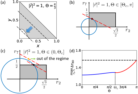
Figure 7: Illustration of the proof of Theorem 5, including (a) minimization of $x+y$, (b) maximization of $\frac{1}{\sqrt{3}}r_{2}+r_{7}$ for $|\vec{r}|^{2}=1$ and $\Theta\in[\Theta_{\mathrm{c}},\pi]$, (c) maximization of $\frac{1}{\sqrt{3}}r_{2}+r_{7}$ for $|\vec{r}|^{2}=1$ and $\Theta\in(0,\Theta_{\mathrm{c}}]$, and (d) $\max_{r_{2},r_{7}}\Delta\tau_{\mathrm{BD}}$ as a function of target $\Theta$. Here $\Theta_{\mathrm{c}}=2\arccos(1/\sqrt{3})$.

Conditions (121) and (122) are not direct constraints on $r_{2}$ and $r_{7}$, but on $x$ and $y$. Since $r^{2}_{2}+r^{2}_{7}=|\vec{r}|^{2}-x-y$, these constraints can affect only the value of $r^{2}_{2}+r^{2}_{7}$. Hence, the first optimization in this case is to minimize $x+y$, which corresponds to the maximum $r^{2}_{2}+r^{2}_{7}$. In the regime given by inequalities (121) and (122), as illustrated in Fig. 7(a) (we take these specific values of $|\vec{r}|^{2}$ and $\Theta$ only for demonstration; the calculation is valid for any value), different values of $x+y$ mean different position of the dashed black line in the plot. It is obvious that the minimum value is attained when the line is closest to the original point, which gives $\min\,x+y=|\vec{r}|^{2}\sin^{2}(\frac{\Theta}{2})$:

$$\max_{x,y}\,r^{2}_{2}+r^{2}_{7}=|\vec{r}|^{2}\cos^{2}\left(\frac{\Theta}{2}\right).$$ (129)

The expression above can be further optimized with respect to $|\vec{r}|^{2}$, i.e., $\max_{|\vec{r}|^{2}}\,r^{2}_{2}+r^{2}_{7}=\cos^{2}(\frac{\Theta}{2})$. Next, we need to optimize the value $\frac{1}{\sqrt{3}}r_{2}+r_{7}$ with the constraint $r^{2}_{2}+r^{2}_{7}=\cos^{2}(\frac{\Theta}{2})$. Due to the semidefinite property of density matrix discussed in Appendix D.1, there we have $r_{7}\leq 1/2$ and $r_{2}\leq\sqrt{3}/2$, as the gray areas shown in Figs. 7(b) and 7(c). Also, the constraint equation $r^{2}_{2}+r^{2}_{7}=\cos^{2}(\frac{\Theta}{2})$ is a circle (blue circles in the plots). The dashed red line represents $\frac{1}{\sqrt{3}}r_{2}+r_{7}=c$ with $c$ a constant. Regardless of the constraints $r_{7}\leq 1/2$ and $r_{2}\leq\sqrt{3}/2$, the maximum value of $\frac{1}{\sqrt{3}}r_{2}+r_{7}$ is always attained (denoted by the black dot) with the dashed red line being the tangent line of the circle. The values of $r_{2}$ and $r_{7}$ for this crossover point are

$$r_{2}=\frac{1}{2}\cos\left(\frac{\Theta}{2}\right),\leavevmode\nobreak\ r_{7}=\frac{\sqrt{3}}{2}\cos\left(\frac{\Theta}{2}\right).$$ (130)

Now let us take into account the constraint on $r_{2}$ and $r_{7}$. For large values of $\Theta$, the crossover point stays in the gray area, as shown in Fig. 7(b), then the maximum value of $\frac{1}{\sqrt{3}}r_{2}+r_{7}$ is attained by this point. For small values of $\Theta$, it is possible that the value of $r_{7}$ for this point [orange point in Fig. 7(c)] is out of the gray area. In this case the maximum value is attained by the point on the circle with $r_{7}=1/2$. The critical target $\Theta_{\mathrm{c}}$ satisfies $\frac{\sqrt{3}}{2}\cos\left(\frac{\Theta_{\mathrm{c}}}{2}\right)=\frac{1}{2}$, which gives $\Theta_{\mathrm{c}}=2\arccos(\frac{1}{\sqrt{3}})$. Thus, in the case of $\Theta\in[\Theta_{\mathrm{c}},\pi]$, $\max\,\Delta\tau_{\mathrm{BD}}$ reads

$$\max_{r_{2},r_{7}}\,\Delta\tau_{\mathrm{BD}}=\frac{\sqrt{3}\Theta}{2\sqrt{1-2\cos\Theta}},$$ (131)

and in the case $\Theta\in(0,\Theta_{\mathrm{c}}]$, it is

$$\max_{r_{2},r_{7}}\,\Delta\tau_{\mathrm{BD}}=\frac{\Theta}{2\sqrt{1-\frac{1}{4}\left[\sqrt{\frac{1}{3}(1+2\cos\Theta)}+1\right]^{2}}}.$$ (132)

Both Eqs. (131) and (132) are plotted in Fig. 7(d) as a function of $\Theta$. It can be seen that the maximum value with respect to $\Theta$ is attained at $\Theta=\pi$, and the corresponding value of $\Delta\tau_{\mathrm{BD}}$ is $\pi/2$. Hence, one can obtain that

$$\Delta\tau_{\mathrm{BD}}\leq\frac{\pi}{2}$$ (133)

for any legitimate values of $|\vec{r}|^{2}$ and $\Theta$. Theorem 5 is then proved. $\blacksquare$

D.4 Analysis and proof of Theorem 6

With Theorem 5, we need to consider only the solutions of Eqs. (112) and (114) within the regime $(0,\frac{\pi}{2}]$ as the solutions not in this regime are obviously larger than $\tau_{\mathrm{BD}}$. Now we compare the values of $\cos(\Delta t)$ in Eqs. (112) and (114) with $\cos(\Delta\tau_{\mathrm{BD}})$. We first consider Eq. (112), i.e., $x=0$. In this case, when $\Theta\geq\frac{\pi}{2}$, there is

$$\frac{1}{y}|\vec{r}|^{2}(1-\cos\Theta)=\frac{|\vec{r}|^{2}(1-\cos\Theta)}{|\vec{r}|^{2}-r^{2}_{2}-r^{2}_{7}}\geq 1,$$ (134)

indicating that $\cos(\Delta t)\leq 0$. Therefore, $t\geq\tau_{\mathrm{BD}}$ in this case. When $\Theta<\pi/2$, if $r^{2}_{2}+r^{2}_{7}\in[|\vec{r}|^{2}\cos\Theta,\frac{1}{2}|\vec{r}|^{2}(1+\cos\Theta)]$, $\cos(\Delta t)$ is also negative and then $t\geq\tau_{\mathrm{BD}}$. Therefore, the only problem left is that if this inequality is still valid for $r^{2}_{2}+r^{2}_{7}\in[0,|\vec{r}|^{2}\cos\Theta]$. That is equivalent to proving the expression

$$\cos\left(\frac{\Theta}{2\sqrt{1-\left(\frac{1}{\sqrt{3}}r_{2}+r_{7}\right)^{2}}}\right)+\frac{|\vec{r}|^{2}(1-\cos\Theta)}{|\vec{r}|^{2}-r^{2}_{2}-r^{2}_{7}}$$ (135)

is larger than 1. In this expression, the minimum value with respect to $|\vec{r}|^{2}$ is attained at $|\vec{r}|^{2}=1$. With this condition, we further use a two-step method to locate the minimum value of the expression above. The first step is to optimize $\frac{1}{\sqrt{3}}r_{2}+r_{7}$ with a fixed value of $r^{2}_{2}+r^{2}_{7}$, i.e., $r^{2}_{2}+r^{2}_{7}=c$ with $c$ a constant. Then the second step is to optimize $c$. In the first step, when $\cos\Theta\leq\frac{1}{3}$, the maximum value of $\frac{1}{\sqrt{3}}r_{2}+r_{7}$ is $\frac{2\sqrt{c}}{\sqrt{3}}$, which is attained by the tangent line on the circle with $r_{2}=\frac{\sqrt{c}}{2}$ and $r_{7}=\frac{\sqrt{3c}}{2}$, as discussed in the proof of Theorem 5. In this case, the minimum value of Eq. (135) reduces to

$$\cos\left(\frac{\Theta}{2\sqrt{1-\frac{4}{3}c}}\right)+\frac{1-\cos\Theta}{1-c}:=h_{1}.$$ (136)

When $\cos\Theta>\frac{1}{3}$, the expression still keeps to be the one above for the case $c\in[0,\frac{1}{3}]$. Whereas for $c\in[\frac{1}{3},\cos\Theta]$, the maximum value of $\frac{1}{\sqrt{3}}r_{2}+r_{7}$ is attained by $r_{2}=\sqrt{c-\frac{1}{4}}$ and $r_{7}=\frac{1}{4}$, and the minimum value of Eq. (135) reduces to

$$\cos\!\left(\frac{\Theta}{2\sqrt{1\!-\!\left[\frac{1}{2}\!+\!\sqrt{\frac{1}{3}(c\!-\!\frac{1}{4})}\right]^{2}}}\right)\!+\!\frac{1\!-\!\cos\Theta}{1\!-\!c}:=h_{2}.$$ (137)

The minimum value of $h_{1}$ and $h_{2}$ with respect to $c$, i.e., $\min_{c}h_{1}$ (solid blue line) and $\min_{c}h_{2}$ (dash-dotted red line), are given in Fig. 8(a) as a function of $\Theta$. It can be seen that in both cases the minimum values for any $\Theta$ is not smaller than one (dashed black line). Therefore, Eq. (135) is indeed always larger than 1 and $t\geq\tau_{\mathrm{BD}}$ holds here.

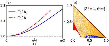
Figure 8: (a) Minimum values of $h_{1}$ and $h_{2}$ with respect to $c$ ($\min_{c}h_{1}$ and $\min_{c}h_{2}$) as a function of $\Theta$. (b) Numerical test of the violation of $t\geq\tau_{\mathrm{BD}}$ in the case $|\vec{r}|^{2}=1$ and $\Theta=\pi/3$. The blue and orange dots represent the states that $t\geq\tau_{\mathrm{BD}}$ is violated or not. The red (dark gray) areas in online (print) version are the regimes that $t\geq\tau_{\mathrm{BD}}$ is guaranteed to hold.

In the case that $x\neq 0$, we need to compare Eq. (114) with $\cos(\Delta\tau_{\mathrm{BD}})$. It is obvious that the solution $f_{-}$ is negative and the corresponding $\Delta t$ is larger than $\pi/2$, indicating that $t\geq\tau_{\mathrm{BD}}$. With respect to the solution $f_{+}$, we first consider a simple case that $r_{2}=r_{7}=0$, which means the diagonal entries of the density matrix are all $1/3$. In this case, $\cos(\Delta\tau_{\mathrm{BD}})$ reduces to $\cos(\frac{\Theta}{2})$ and $f_{+}$ reduces to

$$f_{+}=\frac{-y+\sqrt{16x^{2}\cos^{2}\left(\frac{\Theta}{2}\right)+8xy\cos\Theta+y^{2}}}{4x}.$$ (138)

A non-negative $\cos(\frac{\Theta}{2})-f_{+}$ means

$$4x\cos\left(\frac{\Theta}{2}\right)+y\geq\sqrt{16x^{2}\cos^{2}\left(\frac{\Theta}{2}\right)+8xy\cos\Theta+y^{2}}.$$

As both sides are positive, this inequality can be further simplified by taking the square on both sides, which is of the form

$$8xy\left[\cos\left(\frac{\Theta}{2}\right)-\cos\Theta\right]\geq 0.$$ (139)

This inequality naturally holds since $\Theta\in(0,\pi]$ and $x,y\geq 0$. Hence, $t\geq\tau_{\mathrm{BD}}$ for the states with $r_{2}=r_{7}=0$. In the meantime, in the regime $2x+y\leq 2|\vec{r}|^{2}\sin^{2}(\frac{\Theta}{2})$, $f_{+}$ is still negative. Hence, in the crossover regimes between (121), (122) and $2x+y\leq 2|\vec{r}|^{2}\sin^{2}(\frac{\Theta}{2})$, $t$ is always not smaller than $\tau_{\mathrm{BD}}$.

All the three regimes discussed above are plotted in Fig. 8(b) as the red (dark gray) areas. In the regime $2x+y\geq 2|\vec{r}|^{2}\sin^{2}(\frac{\Theta}{2})$, the situation is a little complicated. Now we first consider the case that $x$ and $y$ are fixed, which means $x+y$ is also fixed. Due to the fact $r^{2}_{2}+r^{2}_{7}=|\vec{r}|^{2}-x-y$, this condition indicates $r^{2}_{2}+r^{2}_{7}=c$ is also fixed ($c$ a real constant). Then according to the discussion in the proof of Theorem 5, the maximum value of $\tau_{\mathrm{BD}}$ becomes

$$\max_{r_{2},r_{7}}\,\tau_{\mathrm{BD}}=\frac{\Theta}{2\Delta\sqrt{1-\frac{4}{3}(|\vec{r}|^{2}-x-y)}}:=\tau_{\mathrm{a},1}$$ (140)

for $x+y\geq|\vec{r}|^{2}-1/3$ and

$$\max_{r_{2},r_{7}}\,\tau_{\mathrm{BD}}\!=\!\frac{\Theta}{2\Delta\sqrt{1\!-\!\left[\frac{1}{2}+\sqrt{\frac{1}{3}(|\vec{r}|^{2}\!-\!x\!-\!y\!-\!\frac{1}{4})}\right]^{2}}}\!:=\!\tau_{\mathrm{a},2}$$ (141)

for $x+y\leq|\vec{r}|^{2}-1/3$. Since the solutions of evolution time $t$ (to reach the target $\Theta$) are related only to $x$ and $y$, $t$ is fixed once $x$ and $y$ are fixed. If $t$ is indeed larger than $\tau_{\mathrm{a},1}$ and $\tau_{\mathrm{a},2}$, then for all the states within the circle $r^{2}_{2}+r^{2}_{7}=c$, $\tau_{\mathrm{BD}}$ is a valid lower bound. Otherwise, $\tau_{\mathrm{BD}}$ fails to be a lower bound at least for the states on the circle. To provide an intuitive picture of this, we randomly generate 10000 states in the regime $2x+y\geq 2|\vec{r}|^{2}\sin^{2}(\Theta/2)$ in the case of $|\vec{r}|^{2}=1$ and $\Theta=\pi/3$, as shown in Fig. 8(b), to test if $\tau_{\mathrm{a},1}$ and $\tau_{\mathrm{a},2}$ are lower than $t$. It can be seen that though $\tau_{\mathrm{BD}}$ remains a valid lower bound for most states (orange dots), the violation (blue dots) indeed happens. The borderline is nothing but the equation

$$\cos(\Delta\tau_{\mathrm{a,i}})-f_{+}=0,$$ (142)

where $i=1$ for $x+y\geq|\vec{r}|^{2}-1/3$ and $i=2$ for $x+y\leq|\vec{r}|^{2}-1/3$. Substituting the expression of $f_{+}$ in Eq. (114) into the equation above, it reduces to

$$x\sin^{2}(\Delta\tau_{\mathrm{a},i})+y\sin^{2}\left(\frac{\Delta\tau_{\mathrm{a},i}}{2}\right)=|\vec{r}|^{2}\sin^{2}\!\left(\frac{\Theta}{2}\right).$$ (143)

Hence, in the regime

$$x\sin^{2}(\Delta\tau_{\mathrm{a},i})+y\sin^{2}\left(\frac{\Delta\tau_{\mathrm{a},i}}{2}\right)\leq|\vec{r}|^{2}\sin^{2}\!\left(\frac{\Theta}{2}\right),$$ (144)

the Bhatia-Davis formula is a valid lower bound.

Furthermore, due to the fact that the violation regime

$$x\sin^{2}(\Delta\tau_{\mathrm{a},i})+y\sin^{2}\left(\frac{\Delta\tau_{\mathrm{a},i}}{2}\right)\geq|\vec{r}|^{2}\sin^{2}\!\left(\frac{\Theta}{2}\right)$$ (145)

is within the regime $y\leq 4x$. Together with Eqs. (121) and (122), the full regime in which $\tau_{\mathrm{BD}}$ is a valid lower bound is

$$\begin{cases}y\geq 4|\vec{r}|\sin\left(\frac{\Theta}{2}\right)\sqrt{x}-4x,\\ y\geq 4x,\\ y\geq|\vec{r}|^{2}\sin^{2}\left(\frac{\Theta}{2}\right),\\ y\leq|\vec{r}|^{2}-x,\end{cases}$$ (146)

and

$$\begin{cases}y\geq 4|\vec{r}|\sin\left(\frac{\Theta}{2}\right)\sqrt{x}-4x,\\ y\leq 4x,\\ y\leq|\vec{r}|^{2}-x,\\ y\sin^{2}(\frac{\Delta\tau_{\mathrm{a},i}}{2})\leq|\vec{r}|^{2}\sin^{2}\!(\frac{\Theta}{2})-x\sin^{2}(\Delta\tau_{\mathrm{a},i}).\end{cases}$$ (147)

Theorem 6 is then proved. $\blacksquare$

References

- (1) L. Mandelstam and I. Tamm, The uncertainty relation between energy and time in nonrelativistic quantum mechanics, J. Phys. 9, 249 (1945).
- (2) S. Deffner and S. Campbell, Quantum speed limits: From Heisenberg’s uncertainty principle to optimal quantum control, J. Phys. A: Math. Theor. 50, 453001 (2017).
- (3) N. Margolus and L. B. Levitin, The maximum speed of dynamical evolution, Physica D 120, 188 (1998).
- (4) V. Giovannetti, S. Lloyd, and L. Maccone, The speed limit of quantum unitary evolution, J. Opt. B 6, 807 (2004).
- (5) M. M. Taddei, B. M. Escher, L. Davidovich, and R. L. de Matos Filho, Quantum Speed Limit for Physical Processes, Phys. Rev. Lett. 110, 050402 (2013).
- (6) A. del Campo, I. L. Egusquiza, M. B. Plenio, and S. F. Huelga, Quantum Speed Limits in Open System Dynamics, Phys. Rev. Lett. 110 050403 (2013).
- (7) S. Deffner and E. Lutz, Quantum Speed Limit for Non-Markovian Dynamics, Phys. Rev. Lett. 111 010402 (2013).
- (8) Z. Sun, J. Liu, J. Ma, and X. Wang, Quantum speed limit for Non-Markovian dynamics without rotating-wave approximation, Sci. Rep. 5, 8444 (2015).
- (9) I. Marvian and D. A. Lidar, Quantum Speed Limits for Leakage and Decoherence, Phys. Rev. Lett. 115, 210402 (2015).
- (10) N. Mirkin, F. Toscano, and D. A. Wisniacki, Quantum-speed-limit bounds in an open quantum evolution, Phys. Rev. A 94, 052125 (2016).
- (11) L. P. García-Pintos and A. del Campo, Quantum speed limits under continuous quantum measurements, New J. Phys. 21, 033012 (2019).
- (12) F. Campaioli, F. A. Pollock, F. C. Binder, and K. Modi, Tightening Quantum Speed Limits for Almost All States, Phys. Rev. Lett. 120, 060409 (2018).
- (13) F. Campaioli, F. A. Pollock, and K. Modi, Tight, robust, and feasible quantum speed limits for open dynamics, Quantum 3, 168 (2019).
- (14) A. Chenu, M. Beau, J. Cao, and A. del Campo, Quantum Simulation of Generic Many-Body Open System Dynamics Using Classical Noise, Phys. Rev. Lett. 118, 140403 (2017).
- (15) M. Beau, J. Kiukas, I. L. Egusquiza, and A. del Campo, Nonexponential quantum decay under environmental decoherence, Phys. Rev. Lett. 119, 130401 (2017).
- (16) X. Cai and Y. Zheng, Quantum dynamical speedup in a nonequilibrium environment, Phys. Rev. A 95, 052104 (2017).
- (17) D. V. Villamizar and E. I. Duzzioni, Quantum speed limit for a relativistic electron in a uniform magnetic field, Phys. Rev. A 92, 042106 (2015).
- (18) S. Sun and Y. Zheng, Distinct Bound of the Quantum Speed Limit via the Gauge Invariant Distance, Phys. Rev. Lett. 123, 180403 (2019).
- (19) X. Meng, C. Wu, and H. Guo, Minimal evolution time and quantum speed limit of non-Markovian open systems, Sci. Rep. 5, 16357 (2015).
- (20) N. Mirkin, M. Larocca, and D. Wisniacki, Quantum metrology in a non-Markovian quantum evolution, Phys. Rev. A 102, 022618 (2020).
- (21) Y.-J. Zhang, W. Han, Y.-J. Xia, J.-P. Cao, and H. Fan, Quantum speed limit for arbitrary initial states, Sci. Rep. 4, 4890 (2014).
- (22) C. Liu, Z.-Y. Xu, and S. Zhu, Quantum-speed-limit time for multiqubit open systems, Phys. Rev. A 91, 022102 (2015).
- (23) D. Mondal, C. Datta, and S. Sazim, Quantum coherence sets the quantum speed limit for mixed states, Phys. Lett. A 380, 689-695 (2016).
- (24) S.-x. Wu and C.-s. Yu, Quantum speed limit for a mixed initial state, Phys. Rev. A 98, 042132 (2018).
- (25) V. Giovannetti, S. Lloyd, and L. Maccone, Quantum limits to dynamical evolution, Phys. Rev. A 67, 052109 (2003).
- (26) V. Giovannetti, S. Lloyd, and L. Maccone, Quantum Metrology, Phys. Rev. Lett. 96, 010401 (2006).
- (27) M. Beau and A. del Campo, Nonlinear quantum metrology of many-body open systems, Phys. Rev. Lett. 119, 010403 (2017).
- (28) T. Caneva, M. Murphy, T. Calarco, R. Fazio, S. Montangero, V. Giovannetti, and G. E. Santoro, Optimal Control at the Quantum Speed Limit, Phys. Rev. Lett. 103, 240501 (2009).
- (29) G. C. Hegerfeldt, Driving at the Quantum Speed Limit: Optimal Control of a Two-Level System, Phys. Rev. Lett. 111, 260501 (2013).
- (30) K. Funo, J.-N. Zhang, C. Chatou, K. Kim, M. Ueda, and A. del Campo, Universal Work Fluctuations During Shortcuts to Adiabaticity by Counterdiabatic Driving, Phys. Rev. Lett. 118, 100602 (2017).
- (31) S. Campbell and S. Deffner, Trade-Off Between Speed and Cost in Shortcuts to Adiabaticity Phys. Rev. Lett. 118, 100601 (2017).
- (32) P. M. Poggi, Geometric quantum speed limits and short-time accessibility to unitary operations, Phys. Rev. A 99, 042116 (2019).
- (33) M. Heyl, Quenching a quantum critical state by the order parameter: Dynamical quantum phase transitions and quantum speed limits, Phys. Rev. B 95, 060504(R) (2017).
- (34) Y. Shao, B. Liu, M. Zhang, H. Yuan, and J. Liu, Operational definition of a quantum speed limit, Phys. Rev. Research 2, 023299 (2020).
- (35) J. M. Epstein and K. B. Whaley, Quantum speed limits for quantum-information-processing tasks, Phys. Rev. A 95, 042314 (2017).
- (36) D. Girolami, How Difficult is it to Prepare a Quantum State? Phys. Rev. Lett. 122, 010505 (2019).
- (37) S. Ashhab, P. C. de Groot, and F. Nori, Speed limits for quantum gates in multiqubit systems, Phys. Rev. A 85, 052327 (2012).
- (38) D. P. Pires, M. Cianciaruso, L. C. Céleri, G. Adesso, and D. O. Soares-Pinto, Generalized Geometric Quantum Speed Limits, Phys. Rev. X 6, 021031 (2016).
- (39) M. Bukov, D. Sels, and A. Polkovnikov, Geometric Speed Limit of Accessible Many-Body State Preparation, Phys. Rev. X 9, 011034 (2019).
- (40) S. Sun, Y. Peng, X. Hu, and Y. Zheng, Quantum Speed Limit Quantified by the Changing Rate of Phase, Phys. Rev. Lett. 127, 100404 (2021).
- (41) I. Marvian, R. W. Spekkens, and P. Zanardi, Quantum speed limits, coherence, and asymmetry Phys. Rev. A 93, 052331 (2016).
- (42) N. Margolus, The finite-state character of physical dynamics, arXiv:1109.4994 (2011).
- (43) B. Shanahan, A. Chenu, N. Margolus, and A. del Campo, Quantum Speed Limits across the Quantum-to-Classical Transition, Phys. Rev. Lett. 120, 070401 (2018).
- (44) M. Okuyama and M. Ohzeki, Quantum Speed Limit is Not Quantum, Phys. Rev. Lett. 120, 070402 (2018).
- (45) S. Amari, Information Geometry and Its Applications, Applied Mathematical Sciences 194, (Springer Japan, 2016).
- (46) G. Ness, M. R. Lam, W. Alt, D. Meschede, Y. Sagi, and A. Alberti, Observing crossover between quantum speed limits, arXiv:2104.05638.
- (47) R. Bhatia and C. Davis, A Better Bound on the Variance, Am. Math. Monthly 107, 353–357 (2000).
- (48) L. B. Levitin and T. Toffoli, Fundamental Limit on the Rate of Quantum Dynamics: The Unified Bound Is Tight, Phys. Rev. Lett. 103, 160502 (2009).
- (49) S. Becker, N. Datta, L. Lami, and C. Rouzé, Energy-Constrained Discrimination of Unitaries, Quantum Speed Limits, and a Gaussian Solovay-Kitaev Theorem, Phys. Rev. Lett. 126, 190504 (2021).
- (50) M. Kitagawa and M. Ueda, Squeezed spin states, Phys. Rev. A 47, 5138 (1993).
- (51) J. Ma, X. Wang, C. P. Sun, and F. Nori, Quantum spin squeezing, Phys. Rep. 509, 89-165 (2011).
- (52) G.-R. Jin, Y.-C. Liu, and W.-M. Liu, Spin squeezing in a generalized one-axis twisting model, New J. Phys. 11, 073049 (2009).
- (53) H.-P. Breuer and F. Petruccione, The Theory of Open Quantum Systems (Oxford University Press, Oxford, 2007).
- (54) M. Hübner, Explicit computation of the Bures distance for density matrices, Phys. Lett. A 163, 239-242 (1992).
- (55) M. Hübner, Computation of Uhlmann’s parallel transport for density matrices and the Bures metric on three-dimensional Hilbert space, Phys. Lett. A 179, 226-230 (1993).
- (56) G. Tóth and I. Apellaniz, Quantum metrology from a quantum information science perspective, J. Phys. A: Math. Theor. 47, 424006 (2014).
- (57) J. Liu, H. Yuan, X.-M. Lu, and X. Wang, Quantum Fisher information matrix and multiparameter estimation, J. Phys. A: Math. Theor. 53, 023001 (2020).