To adjust or not to adjust? Estimating the average treatment effect in randomized experiments with missing covariates

Abstract

Complete randomization allows for consistent estimation of the average treatment effect based on the difference in means of the outcomes without strong modeling assumptions on the outcome-generating process. Appropriate use of the pretreatment covariates can further improve the estimation efficiency. However, missingness in covariates is common in experiments and raises an important question: should we adjust for covariates subject to missingness, and if so, how? The unadjusted difference in means is always unbiased. The complete-covariate analysis adjusts for all completely observed covariates and improves the efficiency of the difference in means if at least one completely observed covariate is predictive of the outcome. Then what is the additional gain of adjusting for covariates subject to missingness? A key insight is that the missingness indicators act as fully observed pretreatment covariates as long as missingness is not affected by the treatment, and can thus be used in covariate adjustment to bring additional estimation efficiency. This motivates adding the missingness indicators to the regression adjustment, yielding the missingness-indicator method as a well-known but not so popular strategy in the literature of missing data. We recommend it due to its many advantages. First, it removes the dependence of the regression-adjusted estimators on the imputed values for the missing covariates. Second, it improves the estimation efficiency of the complete-covariate analysis and the regression analysis based on only the imputed covariates. Third, it does not require modeling the missingness mechanism and yields a consistent and efficient estimator even if the missing-data mechanism is related to the missing covariates and unobservable potential outcomes. Lastly, it is easy to implement via standard software packages for least squares. We also propose modifications to the missingness-indicator method based on asymptotic and finite-sample considerations. To reconcile the conflicting recommendations in the missing data literature, we analyze and compare various strategies for analyzing randomized experiments with missing covariates under the design-based framework. This framework treats randomization as the basis for inference and does not impose any modeling assumptions on the outcome-generating process and missing-data mechanism.

Keywords: efficiency; imputation; missingness pattern; randomized controlled trial; regression adjustment; robust standard error

Introduction

Ever since the seminal work of Fisher (1935), randomization has become the gold standard for estimating treatment effects without strong modeling assumptions. It justifies the simple comparison of outcome means across treatment groups (Neyman 1923) and allows for additional gains in efficiency by appropriate adjustment for pretreatment covariates (Fisher 1935; Lin 2013). In particular, Lin (2013) showed that the coefficient of the treatment from the ordinary least squares (ols) fit of the outcome on the treatment, centered covariates, and their interactions is a consistent and asymptotically efficient estimator for the average treatment effect, and moreover, the associated Eicker–Huber–White robust standard error is a convenient approximation to the true standard error. Importantly, Lin (2013)’s theory holds even if the linear model is misspecified.

Missingness in covariates, however, is ubiquitous in field experiments in biomedical and social sciences, and imposes a dilemma to subsequent analyses. We can simply ignore the covariates and proceed with the unadjusted difference in means, which is unbiased and consistent under complete randomization. An immediate improvement is the complete-covariate analysis that adjusts for only the subset of covariates that are observed for all units. It is more efficient than the unadjusted estimator if at least one completely observed covariate is prognostic to the outcome. Although some existing methods for missing covariates are likely to further improve efficiency, they rely on additional modeling assumptions on the outcome model or the missingness mechanism (Rubin 1987; Little 1992; Ibrahim et al. 2005; Little and Rubin 2019). Due to the unverifiable additional assumptions, these more sophisticated methods do not strictly dominate the simpler unadjusted estimator and complete-covariate analysis in randomized experiments. Then a natural question arises: should we adjust for the missing covariates or not?

Our answer to the question above is yes. We propose to simply impute the missing covariates with zeros, augment the imputed covariates with the missingness indicators, and then apply Lin (2013)’s estimator for covariate adjustment. This method becomes intuitive if the missingness is not affected by the treatment such that we can view the missingness indicators as a set of fully observed pretreatment covariates. The resulting missingness-indicator method has many advantages. First, unlike the complete-case analysis that discards units with any missing covariates, it is consistent without assuming that the complete cases are representative of the whole population and can be much more efficient when the proportion of missingness is substantial. Second, unlike the single imputation method, it is invariant to the imputed values for the missing covariates, so the convenient choice of imputing by zeros results in no loss of generality. Third, it is asymptotically more efficient than the complete-covariate analysis and single imputation if the missingness indicators are prognostic to the outcome. Fourth, it does not require modeling of the missingness mechanism and, surprisingly, remains consistent for the average treatment effect even when the missingness mechanism depends on the missing covariates and unobservable potential outcomes, a scenario analogous to missing not at random under the super-population framework (Rubin 1976; Little and Rubin 2019). Lastly, it can be easily implemented via standard software packages for ols and robust standard errors.

This missingness-indicator method is not entirely new. Cohen and Cohen (1975, Chapter 7) proposed to use it in regression analysis; Rosenbaum and Rubin (1984, Appendix B) suggested it in matching for causal inference with observational studies. See D’Agostino and Rubin (2000), Rosenbaum (2010, Sections 9.4 and 13.4), Mattei (2009), and Fogarty et al. (2016) for applications of this method to observational studies, and see Anderson et al. (1983) and Groenwold et al. (2012) for a review. However, this method was criticized by Greenland and Finkle (1995), Donders et al. (2006), and Yang et al. (2019). Greenland and Finkle (1995) evaluated this method in the context of logistic regression in observational studies and reported severe bias even when the data are missing completely at random; Donders et al. (2006) offered a similar discussion. Yang et al. (2019) argued that the underlying assumption in Rosenbaum and Rubin (1984) for this method is unreasonable in observational studies. Miettinen (1985) acknowledged its convenience for application, but also pointed out its limitation of representing only partial control when applied to confounders. However, our recommendation is not in contradiction with the existing literature. The fundamental difference between randomized experiments and observational studies explains the seemingly contradictory recommendations. Although the missingness-indicator method can be problematic in observational studies, it has appealing theoretical guarantees mentioned above in randomized experiments. Randomization balances the pretreatment covariates as well as the missingness indicators on average across different treatment groups. Using them in Lin (2013)’s procedure thus ensures consistent and efficient estimation for the average treatment effect. Our results echo White and Thompson (2005) and Carpenter and Kenward (2007, Section 2.4) without assuming that the covariates and outcomes are normally distributed. Rather, we analyze and compare different methods under the design-based framework, also known as the randomization-based framework, free of any modeling assumptions. Therefore, the above theoretical guarantees of the missingness-indicator method hold even if the outcome model is misspecified. This is also a key distinction between our results and those for correctly-specified regression models with missing covariates (Rubin 1987; Little 1992; Robins et al. 1994; Jones 1996; Ibrahim et al. 2005).

Moreover, we propose modifications to the missingness-indicator method based on asymptotic and finite-sample considerations. First, the missingness-pattern method stratifies the data based on the missingness patterns and applies Lin (2013)’s estimator based on the available covariates within each stratum. It is closely related to post-stratification (Miratrix et al. 2013) if we view the type of missingness pattern as a discrete covariate, and can be seen as an extension of the available-covariate analysis proposed by Wilks (1932), Matthai (1951), Glasser (1964), and Haitovsky (1968). The resulting estimator allows for heterogeneous adjustments across different missingness patterns, and thereby promises additional asymptotic efficiency over the missingness-indicator method if the covariates and missingness patterns affect the treatment effects in non-additive ways. We recommend this method if the sample sizes within all missingness patterns are large enough to justify the application of Lin (2013)’s estimator. In finite samples, however, both the missingness-indicator and missingness-pattern methods can have substantial variability due to estimating many regression coefficients when the number of covariates is large. This motivates the complete-case-indicator method and the missingness-count method that augment the imputed covariates with only the scalar complete-case indicator and the missingness-count variable, respectively, instead of all missingness indicators. The resulting estimators may lose asymptotic efficiency but can improve the finite-sample properties.

We start with the completely randomized treatment-control experiment in Section 2, and outline five strategies for handling missing covariates in randomized experiments in Section 3. We analyze and compare their asymptotic properties from the design-based perspective in Section 4. We use simulation and an application to illustrate the methods and theory in Sections 5 and 6. We then extend the theory to cluster randomization and stratified randomization in Section 7. We conclude in Section 8 and relegate all technical details to the Supplementary Material.

The following notation facilitates the discussion. For a finite population $\{(u_{i},v_{i}):i\in\mathcal{I}\}$, let $\bar{u}=|\mathcal{I}|^{-1}\sum_{i\in\mathcal{I}}u_{i}$, $\bar{v}=|\mathcal{I}|^{-1}\sum_{i\in\mathcal{I}}v_{i}$, and $S_{uv}=(|\mathcal{I}|-1)^{-1}\sum_{i\in\mathcal{I}}(u_{i}-\bar{u})(v_{i}-\bar{v})^{\mathrm{\scriptscriptstyle T}}$ be the finite-population means and covariance, respectively. We specify the composition of $\mathcal{I}$ in the context. In the case of $u_{i}=v_{i}$, we also occasionally write $S_{uu}$ as $S_{u}^{2}$. For $v_{i}\in\mathbb{R}$ and $u_{i}\in\mathbb{R}^{J}$, let $v_{i}\sim u_{i}$ denote the ols fit of $v_{i}$ on $u_{i}$ over $i\in\mathcal{I}$. For example, for $\{(Y_{i},Z_{i},x_{i}):i=1,\ldots,N\}$ with $Y_{i}\in\mathbb{R}$, $Z_{i}\in\mathbb{R}$, and $x_{i}\in\mathbb{R}^{J}$, let $Y_{i}\sim 1+Z_{i}+x_{i}$ denote the additive ols fit of $Y_{i}$ on $(1,Z_{i},x_{i})$ over $i=1,\ldots,N$ with regressor vector $(1,Z_{i},x_{i}^{\mathrm{\scriptscriptstyle T}})^{\mathrm{\scriptscriptstyle T}}$; let $Y_{i}\sim 1+Z_{i}+(x_{i}-\bar{x})+Z_{i}(x_{i}-\bar{x})$ denote the fully interacted ols fit of $Y_{i}$ on $\{1,Z_{i},(x_{i}-\bar{x})\}$ over $i=1,\ldots,N$ with centered covariates, $x_{i}-\bar{x}$, and regressor vector $(1,Z_{i},(x_{i}-\bar{x})^{\mathrm{\scriptscriptstyle T}},Z_{i}(x_{i}-\bar{x})^{\mathrm{\scriptscriptstyle T}})^{\mathrm{\scriptscriptstyle T}}$. Importantly, we do not invoke the modeling assumptions for ols, but evaluate the sampling properties of the numerical outputs from the design-based perspective. We focus on the robust standard errors from ols because the classic standard errors do not have the desired design-based properties even in the simple cases (Freedman 2008; Lin 2013).

Basic setup under the treatment-control experiment

2.1 Regression-adjusted estimators with completely observed covariates

Consider an intervention of two levels, $z=0,1$, and a finite population of $N$ units, $i=1,\ldots,N$. Let $Y_{i}(z)$ be the potential outcome of unit $i$ under treatment $z$. The individual treatment effect is $\tau_{i}=Y_{i}(1)-Y_{i}(0)$, and the finite-population average treatment effect is $\tau=N^{-1}\sum_{i=1}^{N}\tau_{i}=\bar{Y}(1)-\bar{Y}(0)$, where $\bar{Y}(z)=N^{-1}\sum_{i=1}^{N}Y_{i}(z)$.

The designer assigns $N_{z}$ units to receive level $z$ with $N_{0}+N_{1}=N$ and $(e_{0},e_{1})=(N_{0}/N,N_{1}/N).$ Let $Z_{i}$ denote the treatment level received by unit $i$, with $Z_{i}=1$ for treatment and $Z_{i}=0$ for control. Complete randomization samples $(Z_{1},\ldots,Z_{N})$ uniformly from all permutations of $N_{1}$ 1’s and $N_{0}$ 0’s. The observed outcome is $Y_{i}=Z_{i}Y_{i}(1)+(1-Z_{i})Y_{i}(0)$ for unit $i$.

Let $\hat{Y}(z)=N_{z}^{-1}\sum_{i:Z_{i}=z}Y_{i}$ be the sample average of the outcomes under treatment $z$. The difference-in-means estimator $\hat{\tau}_{\textsc{n}}=\hat{Y}(1)-\hat{Y}(0)$ is unbiased for $\tau$, and equals the coefficient of $Z_{i}$ from the simple ols fit of $Y_{i}\sim 1+Z_{i}$ over $i=1,\ldots,N$. The presence of covariates affords the opportunity to further improve the efficiency. Let $x_{i}=(x_{i1},\ldots,x_{iJ})^{\mathrm{\scriptscriptstyle T}}$ be the $J$-dimensional covariate vector for unit $i$. Fisher (1935) suggested an estimator $\hat{\tau}_{\textsc{f}}$ for $\tau$, which equals the coefficient of $Z_{i}$ from the additive ols fit $Y_{i}\sim 1+Z_{i}+x_{i}$ over $i=1,\ldots,N$. Lin (2013) recommended an improved estimator, $\hat{\tau}_{\textsc{l}}$, as the coefficient of $Z_{i}$ from the fully interacted ols fit $Y_{i}\sim 1+Z_{i}+(x_{i}-\bar{x})+Z_{i}(x_{i}-\bar{x})$ over $i=1,\ldots,N$ with centered covariates and treatment-covariates interactions, and showed its asymptotic efficiency over $\hat{\tau}_{\textsc{n}}$ and $\hat{\tau}_{\textsc{f}}$. We summarize the results in Lemma 1 below, with the subscripts “n”, “f”, and “l” signifying Neyman (1923), Fisher (1935), and Lin (2013), respectively. We adopt the finite-population design-based framework conditioning on the potential outcomes, but the theory extends to the super-population framework with minor modifications (Tsiatis et al. 2008; Negi and Wooldridge 2021). The following regularity condition is standard for inference under the design-based framework (Li and Ding 2017).

Condition 1.

As $N\to\infty$, (i) $e_{z}$ has a limit in $(0,1)$ for $z=0,1$, (ii) the finite-population first two moments of $\{Y_{i}(0),Y_{i}(1),x_{i}\}_{i=1}^{N}$ have finite limits; the limit of $S_{x}^{2}$ is positive definite, and (iii) there exists a $u_{0}<\infty$ independent of $N$ such that $N^{-1}\sum_{i=1}^{N}\|x_{i}\|_{4}^{4}\leq u_{0}$ and $N^{-1}\sum_{i=1}^{N}Y_{i}^{4}(z)\leq u_{0}$ for $z=0,1$.

Let $\gamma_{{\textsc{l}},z}=(S^{2}_{x})^{-1}S_{xY(z)}$ be the coefficient of $x_{i}$ from the ols fit $Y_{i}(z)\sim 1+x_{i}$ over $i=1,\ldots,N$. Let $\gamma_{\textsc{f}}=e_{0}\gamma_{{\textsc{l}},0}+e_{1}\gamma_{{\textsc{l}},1}$, and let $S_{z,{\textsc{n}}}^{2}$, $S^{2}_{z,{\textsc{f}}}$, and $S^{2}_{z,{\textsc{l}}}$ be the finite-population variances of $\{Y_{i}(z)\}_{i=1}^{N}$, $\{Y_{i}(z)-x_{i}^{\mathrm{\scriptscriptstyle T}}\gamma_{\textsc{f}}\}_{i=1}^{N}$, and $\{Y_{i}(z)-x_{i}^{\mathrm{\scriptscriptstyle T}}\gamma_{{\textsc{l}},z}\}_{i=1}^{N}$, respectively, for $z=0,1$. Let $S_{\tau,{\textsc{n}}}^{2}=S^{2}_{\tau,{\textsc{f}}}$ and $S^{2}_{\tau,{\textsc{l}}}$ be the finite-population variances of $(\tau_{i})_{i=1}^{N}$ and $\{\tau_{i}-x_{i}^{\mathrm{\scriptscriptstyle T}}(\gamma_{{\textsc{l}},1}-\gamma_{{\textsc{l}},0})\}_{i=1}^{N}$, respectively. Condition 1 ensures $e_{z}$, $S^{2}_{z,{\star}}$, and $S^{2}_{\tau,{\star}}$ all have finite limits for $z=0,1$ and ${\star}={\textsc{n}},{\textsc{f}},{\textsc{l}}$. We will also use the same symbols to denote their respective limits when no confusion would arise.

Lemma 1.

Assume complete randomization and Condition 1. We have $\sqrt{N}(\hat{\tau}_{\star}-\tau)\rightsquigarrow\mathcal{N}(0,v_{\star})$ for ${\star}={\textsc{n}},{\textsc{f}},{\textsc{l}}$ with

$$v_{\star}=e_{0}^{-1}S^{2}_{0,{\star}}+e_{1}^{-1}S^{2}_{1,{\star}}-S^{2}_{\tau,{\star}}$$

and $v_{\textsc{l}}\leq v_{\textsc{n}}$, $v_{\textsc{l}}\leq v_{\textsc{f}}$. Further let $\hat{\text{se}}_{\star}$ be the robust standard error of $\hat{\tau}_{\star}$ from the corresponding ols fit. We have $N\hat{\text{se}}^{2}_{\star}-v_{\star}=S^{2}_{\tau,{\star}}+{o_{P}(1)}$ with $S^{2}_{\tau,{\star}}\geq 0$.

Lemma 1 reviews the classic results from Neyman (1923), Freedman (2008), and Lin (2013). The simple, additive, and fully interacted ols fits thus give consistent and asymptotically normal estimators for $\tau$, and the corresponding robust standard errors are asymptotically conservative for estimating the true standard errors. Asymptotically, Lin (2013)’s estimator is the most efficient, whereas Fisher (1935)’s estimator can be even less efficient than the unadjusted difference in means.

Li and Ding (2020) showed that $v_{\textsc{l}}=v_{\textsc{n}}(1-R^{2})$, where $R^{2}$ is the squared multiple correlation between $\hat{\tau}_{\textsc{n}}$ and the difference in means of the covariates, $\hat{\tau}_{x}=\hat{x}(1)-\hat{x}(0)$ with $\hat{x}(z)=N_{z}^{-1}\sum_{i:Z_{i}=z}x_{i}$. Therefore, including more covariates in Lin (2013)’s estimator will never decrease the asymptotic efficiency. Lemma 2 below gives a more general result.

Lemma 2.

Let $\hat{\tau}_{{\textsc{l}}}^{a}$ and $\hat{\tau}_{{\textsc{l}}}^{b}$ be Lin (2013)’s estimators based on covariates $a_{i}$ and $b_{i}$, respectively. Let $A$ and $B$ be the matrices with $a_{i}$ and $b_{i}$ being the $i$th row vectors, respectively. If the column space of $A$ is a subset of that of $B$, then the asymptotic variance of $\hat{\tau}_{{\textsc{l}}}^{a}$ is greater than or equal to that of $\hat{\tau}_{{\textsc{l}}}^{b}$ under complete randomization and Condition 1.

Lemma 2 reduces the comparison of asymptotic efficiency of two Lin (2013)’s estimators to that of the column spaces of the respective covariate matrix. It affords the basis for comparing the asymptotic efficiency of various estimators; see Section 4. In finite samples, however, adjusting for more covariates may increase both bias and variance. This motivates us to consider practical estimators suitable for moderate sample sizes; see Section 7.

2.2 Missing data and running examples

The proposals by Fisher (1935) and Lin (2013) assume the $J$ covariates are fully observed for all $N$ units. Of interest is how to adapt when some covariates are only partially available.

Let $M_{i}=(M_{i1},\ldots,M_{iJ})^{\mathrm{\scriptscriptstyle T}}\in\{0,1\}^{J}$ be the missingness indicators for unit $i$ with $M_{ij}=1$ if $x_{ij}$ is missing and $M_{ij}=0$ if otherwise. The possible values of $M_{i}$ defines $2^{J}$ possible missingness patterns, indexed by $m=(m_{1},\ldots,m_{J})^{\mathrm{\scriptscriptstyle T}}\in\{0,1\}^{J}$. Not all $2^{J}$ missingness patterns need to be present in any given data set. Let $N_{(m)}=N_{(m_{1}\ldots m_{J})}=\sum_{i=1}^{N}1(M_{i}=m)$ be the number of units with missingness pattern $m=(m_{1},\ldots,m_{J})^{\mathrm{\scriptscriptstyle T}}$, and let $\mathcal{M}=\{m:N_{(m)}>0\}$ be the set of missingness patterns that are present in the data set. We use parentheses in the subscript of $N_{(m)}$ to differentiate it from the treatment group sizes, $(N_{0},N_{1})$.

We use the following running examples for illustrating the key concepts throughout the text. For simplicity, we use “obs” and “mis” to denote whether a covariate is observed or missing.

Example 1.

Consider the case with $J=1$ covariate, $x_{i}=x_{i1}$, for $i=1,\ldots,N$. The missingness indicators satisfy $M_{i}=M_{i1}\in\{0,1\}$, and suggest two possible missingness patterns, $m\in\{0,1\}$, with $N_{(0)}=\sum_{i=1}^{N}1(M_{i}=0)=N-\sum_{i=1}^{N}M_{i}$ and $N_{(1)}=\sum_{i=1}^{N}1(M_{i}=1)=\sum_{i=1}^{N}M_{i}$:

missingness pattern $(M_{i})$	$x_{i}$	number of units
0	obs	$N_{(0)}$
1	mis	$N_{(1)}$

Example 2.

Consider the case with $J=2$ covariates, $x_{i}=(x_{i1},x_{i2})^{\mathrm{\scriptscriptstyle T}}$, for $i=1,\ldots,N$. The missingness indicators satisfy $M_{i}=(M_{i1},M_{i2})^{\mathrm{\scriptscriptstyle T}}\in\{0,1\}^{2}$, and suggest $2^{2}=4$ possible missingness patterns, $m=(m_{1},m_{2})^{\mathrm{\scriptscriptstyle T}}\in\{0,1\}^{2}$, with $N_{(m)}=\sum_{i=1}^{N}1(M_{i1}=m_{1},M_{i2}=m_{2})$:

missingness pattern ($M_{i}$)	$x_{i1}$	$x_{i2}$	number of units
$(0,0)^{\mathrm{\scriptscriptstyle T}}$	obs	obs	$N_{(00)}$
$(0,1)^{\mathrm{\scriptscriptstyle T}}$	obs	mis	$N_{(01)}$
$(1,0)^{\mathrm{\scriptscriptstyle T}}$	mis	obs	$N_{(10)}$
$(1,1)^{\mathrm{\scriptscriptstyle T}}$	mis	mis	$N_{(11)}$

Depending on the specific application under consideration, the missingness may or may not depend on the treatment assignment. To simplify the presentation, we start with the case where missingness is unaffected by the treatment assignment in Sections 3 and 4, and then extend to the case where $M_{i}$ can be dependent on $Z_{i}$ in Section 7. Let $M_{i}(z)=(M_{i1}(z),\ldots,M_{iJ}(z))^{\mathrm{\scriptscriptstyle T}}$ be the potential value of $M_{i}$ if unit $i$ were assigned to treatment $z$. Condition 2 below formalizes the notion of treatment-independent missingness in terms of these potential values.

Condition 2.

$M_{i}(0)=M_{i}(1)=M_{i}$ for all $i=1,\ldots,N$.

Condition 2 states that the potential missingness does not depend on the treatment assignment such that the $M_{i}$’s are effectively a set of fully observed pretreatment covariates unaffected by $Z_{i}$’s. If the missingness happens before the treatment assignment, it cannot be affected by the treatment and Condition 2 holds automatically. If the covariates are collected retrospectively after the experiment, the missingness indicators may be affected by the treatment and Condition 2 may be violated. The former case is arguably more common in randomized experiments (White and Thompson 2005; Carpenter and Kenward 2007; Sullivan et al. 2018). It is thus our focus.

Five strategies for handling missing covariates

We focus on five strategies for handling missing covariates. The simplest strategies are the complete-case analysis that utilizes units with completely observed covariates and the complete-covariate analysis that utilizes covariates completely observed for all units. We then review the single imputation method that first fills in the missing covariates with some values and then proceeds with the standard complete-data analysis with the imputed data. When the missingness indicators act as pretreatment covariates, it is also natural to include them directly in ols, motivating the missingness-indicator method. We end this section by proposing the missingness-pattern method as an alternative to the missingness-indicator method that ensures additional asymptotic efficiency.

3.1 Complete-case analysis

Most standard software routines adopt the complete-case analysis as default by dropping all units with any missingness in covariates. Let $C_{i}=1(M_{i}=0_{J})$ be the complete-case indicator for unit $i$, with $C_{i}=1$ if and only if the $J$-vector $x_{i}$ is fully observed. The complete-case analysis uses only the $N^{\textup{cc}}=\sum_{i=1}^{N}C_{i}$ complete cases, indexed by $\{i:C_{i}=1\}$. Let $\bar{x}^{\textup{cc}}=(N^{\textup{cc}})^{-1}\sum_{i:C_{i}=1}x_{i}$ be the average of $x_{i}$’s over the complete cases. The resulting analysis fits

$$Y_{i}\sim 1+Z_{i}+x_{i},$$ (1)

$$Y_{i}\sim 1+Z_{i}+(x_{i}-\bar{x}^{\textup{cc}})+Z_{i}(x_{i}-\bar{x}^{\textup{cc}})$$ (2)

over $\{i:C_{i}=1\}$ under the additive and fully interacted specifications, respectively, and uses the coefficients of $Z_{i}$, denoted by $\hat{\tau}_{{\textsc{f}}}^{\textup{cc}}$ and $\hat{\tau}_{{\textsc{l}}}^{\textup{cc}}$, respectively, to estimate $\tau$.

In Example 1 with $J=1$ covariate, we have $C_{i}=1-M_{i}$ for $i=1,\ldots,N$, and the complete-case analysis uses units with $M_{i}=0$. In Example 2 with $J=2$ covariates, we have $C_{i}=(1-M_{i1})(1-M_{i2})$ for $i=1,\ldots,N$, and the complete-case analysis uses units with $M_{i1}=M_{i2}=0$.

3.2 Complete-covariate analysis

Another straightforward option is the complete-covariate analysis that omits any covariates that are not completely observed for all units. Denote by $\mathcal{J}=\{j:M_{ij}=0\ \text{for}\ i=1,\ldots,N\}$ the set of complete covariates, and let $x_{i}^{\textup{ccov}}=(x_{ij})_{j\in\mathcal{J}}$ be the subvector of $x_{i}$ corresponding to the covariates in $\mathcal{J}$. The complete-covariate analysis fits

$$Y_{i}\sim 1+Z_{i}+x_{i}^{\textup{ccov}},$$ (3)

$$Y_{i}\sim 1+Z_{i}+(x_{i}^{\textup{ccov}}-\bar{x}^{\textup{ccov}})+Z_{i}(x_{i}^{\textup{ccov}}-\bar{x}^{\textup{ccov}})$$ (4)

over $i=1,\ldots,N$ under the additive and fully interacted specifications, respectively, and uses the coefficients of $Z_{i}$, denoted by $\hat{\tau}_{\textsc{f}}^{\textup{ccov}}$ and $\hat{\tau}_{\textsc{l}}^{\textup{ccov}}$, respectively, to estimate $\tau$. In the case of $\mathcal{J}=\emptyset$, both (3) and (4) reduce to $Y_{i}\sim 1+Z_{i}$ with $\hat{\tau}_{\textsc{f}}^{\textup{ccov}}=\hat{\tau}_{\textsc{l}}^{\textup{ccov}}=\hat{\tau}_{\textsc{n}}$.

3.3 Single imputation

The single imputation strategy imputes the missing covariates based on the observed data, and analyzes the imputed data by standard methods. It allows for the inclusion of all cases and covariates in the analysis.

Consider a covariate-wise imputation that imputes all missing $x_{ij}$’s along the $j$th dimension by some prespecified $c_{j}$ that may depend on the observed data. Common choices include $c_{j}=0$ and the covariate-wise observed average $c_{j}=\hat{x}_{j}^{\rm obs}=\sum_{i=1}^{N}(1-M_{ij})x_{ij}/\sum_{i=1}^{N}(1-M_{ij})$. Denote by $x_{i}^{\textup{imp}}(c)=(x^{\textup{imp}}_{i1}(c_{1}),\ldots,x^{\textup{imp}}_{iJ}(c_{J}))^{\mathrm{\scriptscriptstyle T}}$ the resulting imputed covariates with $c=(c_{j})_{j=1}^{J}$ and $x^{\textup{imp}}_{ij}(c_{j})=(1-M_{ij})x_{ij}+M_{ij}c_{j}$. We can proceed with fitting

$$Y_{i}\sim 1+Z_{i}+x_{i}^{\textup{imp}}(c),$$ (5)

$$Y_{i}\sim 1+Z_{i}+\{x_{i}^{\textup{imp}}(c)-\bar{x}^{\textup{imp}}(c)\}+Z_{i}\{x_{i}^{\textup{imp}}(c)-\bar{x}^{\textup{imp}}(c)\}$$ (6)

over $i=1,\ldots,N$, respectively, and estimate $\tau$ by the coefficients of $Z_{i}$, denoted by $\hat{\tau}_{\textsc{f}}^{\textup{imp}}(c)$ and $\hat{\tau}_{\textsc{l}}^{\textup{imp}}(c)$, respectively.

The above covariate-wise imputation enforces identical imputation value for all missing values along the same covariate, and could thus appear quite restrictive at first glance. Other common choices for single imputation include the treatment-specific sample means of the observed covariates (Schemper and Smith 1990) and other conditional sample means of the observed covariates based on either only the observed covariates or both the observed covariates and outcomes (Little 1992). We will nevertheless focus on the simple covariate-wise imputation in this text due to its sufficiency for randomized experiments; see Sullivan et al. (2018), Kayembe et al. (2020), and Kamat and Reiter (2021) for numerical evidence on the insensitivity of standard analyses to imputation methods in randomized experiments. We leave the theory on more sophisticated imputation methods to future work. Moreover, we will show that the robust standard errors from ols are convenient approximations to the true standard errors without any adjustment. Therefore, we also omit the discussion of multiple imputation as a tool to assess imputation uncertainty in general scenarios (Rubin 1987).

3.4 Missingness-indicator method

The missingness-indicator method augments (5) and (6) under single imputation by also including $M_{i}$ as additional regressors to account for the missingness information. In particular, we first impute the missing $x_{ij}$’s by covariate-specific $c_{j}$’s $(j=1,\ldots,J)$, and then fit

$$Y_{i}\sim 1+Z_{i}+x_{i}^{\textup{imp}}(c)+M_{i},$$ (7)

$$Y_{i}\sim 1+Z_{i}+(x_{i}^{\textup{imp}}(c)-\bar{x}^{\textup{imp}}(c))+(M_{i}-\bar{M})+Z_{i}(x_{i}^{\textup{imp}}(c)-\bar{x}^{\textup{imp}}(c))+Z_{i}(M_{i}-\bar{M})$$ (8)

over $i=1,\ldots,N$ to construct the regression estimators as the coefficients of $Z_{i}$, denoted by $\hat{\tau}^{\textup{mim}}_{\textsc{f}}(c)$ and $\hat{\tau}^{\textup{mim}}_{\textsc{l}}(c)$, respectively. This is equivalent to running the additive and fully interacted regressions based on the augmented covariate vector $x_{i}^{\textup{mim}}(c)=(x_{i}^{\textup{imp}}(c)^{\mathrm{\scriptscriptstyle T}},M_{i}^{\mathrm{\scriptscriptstyle T}})^{\mathrm{\scriptscriptstyle T}}\in\mathbb{R}^{2J}$.

Strictly speaking, $M_{ij}=0$ for all $i=1,\ldots,N$ for $j\in\mathcal{J}$ such that we need to include only $M_{ij}$ for the incomplete covariates. In addition, in case $M_{ij}=M_{ij^{\prime}}$ for all $i=1,\ldots,N$ for some $j\neq j^{\prime}$, we need to include only one of them to avoid collinearity. Acknowledging the need to adjust for these complications on a case-by-case basis, we will use $M_{i}$ to represent the vector of missingness indicators added to the model after appropriate adjustment for notational simplicity. This causes little confusion because standard software packages for ols automatically drop redundant regressors.

As it turns out, the resulting point estimators $\hat{\tau}_{\star}^{\textup{mim}}(c)\ ({\star}={\textsc{f}},{\textsc{l}})$ and their associated robust standard errors $\hat{\text{se}}_{\star}^{\textup{mim}}(c)\ ({\star}={\textsc{f}},{\textsc{l}})$ are invariant to the choice of the imputation vector $c$. This is a numeric merit due to the inclusion of the missingness indicators, and allows us to construct $\hat{\tau}_{\star}^{\textup{mim}}(c)$ by simply imputing all missing covariates as 0. We formalize the intuition in Lemma 3 below.

Let $x^{0}_{i}=x_{i}^{\textup{imp}}(0_{J})$ be the imputed covariate vector where we fill in all missing $x_{ij}$’s with 0. Let $\hat{\tau}_{\star}^{\textup{mim}}=\hat{\tau}_{\star}^{\textup{mim}}(0_{J})$ and $\hat{\text{se}}_{\star}^{\textup{mim}}=\hat{\text{se}}_{\star}^{\textup{mim}}(0_{J})$ be the regression estimators and associated robust standard errors from

$$Y_{i}\sim 1+Z_{i}+x_{i}^{0}+M_{i}$$ (10)

$$Y_{i}\sim 1+Z_{i}+(x_{i}^{0}-\bar{x}^{0})+(M_{i}-\bar{M})+Z_{i}(x_{i}^{0}-\bar{x}^{0})+Z_{i}(M_{i}-\bar{M})$$

over $i=1,\ldots,N$, respectively, for ${\star}={\textsc{f}},{\textsc{l}}$. These are effectively regression adjustments with covariates $x_{i}^{\textup{mim}}=((x_{i}^{0})^{\mathrm{\scriptscriptstyle T}},M_{i}^{\mathrm{\scriptscriptstyle T}})^{\mathrm{\scriptscriptstyle T}}$.

Lemma 3.

$\hat{\tau}_{\star}^{\textup{mim}}(c)=\hat{\tau}_{\star}^{\textup{mim}}$ and $\hat{\text{se}}_{\star}^{\textup{mim}}(c)=\hat{\text{se}}_{\star}^{\textup{mim}}$ for ${\star}={\textsc{f}},{\textsc{l}}$ for all $c\in\mathbb{R}^{J}$.

Cohen and Cohen (1975) hinted at the invariance of $\hat{\tau}_{\textsc{f}}^{\textup{mim}}(c)$ to the choice of $c$. Lemma 3 formalizes the results for both $\hat{\tau}_{\textsc{f}}^{\textup{mim}}(c)$ and $\hat{\tau}_{\textsc{l}}^{\textup{mim}}(c)$ as well as their corresponding robust standard errors $\hat{\text{se}}_{\textsc{f}}^{\textup{mim}}(c)$ and $\hat{\text{se}}_{\textsc{l}}^{\textup{mim}}(c)$.

3.5 Missingness-pattern method

The missingness-indicator method factors in information in missingness by including $M_{i}$ as additional regressors in ols. We propose the missingness-pattern method that goes one step further and performs one separate analysis for each missingness pattern based on all available covariates. Let $\rho_{(m)}=N_{(m)}/N$ denote the proportion of units with missingness pattern $m\in\{0,1\}^{J}$. We use Examples 1 and 2 (continued) below with $J=1$ and $J=2$ to illustrate the basic idea, and then formalize the method for general $J$.

Example 1 (continued).

Consider the case of $J=1$ covariate and two missingness patterns. We can fit one additive regression for each missingness pattern to obtain the coefficients of $Z_{i}$ as follows:

1. regress $Y_{i}$ on $(1,Z_{i},x_{i})$ over $\{i:M_{i}=0\}$ to obtain $\hat{\tau}_{{\textsc{f}},(0)}$;

2. regress $Y_{i}$ on $(1,Z_{i})$ over $\{i:M_{i}=1\}$ to obtain $\hat{\tau}_{{\textsc{f}},(1)}=\hat{\tau}_{{\textsc{n}},(1)}$.

The weighted average $\hat{\tau}_{{\textsc{f}}}^{\textup{mp}}=\rho_{(0)}\hat{\tau}_{{\textsc{f}},(0)}+\rho_{(1)}\hat{\tau}_{{\textsc{f}},(1)}$ gives an estimator for $\tau$. Analogously, we can also obtain $\hat{\tau}_{{\textsc{l}}}^{\textup{mp}}$ by running one fully interacted regression for each missingness pattern.

Example 2 (continued).

Consider the case of $J=2$ covariates, $x_{i}=(x_{i1},x_{i2})^{\mathrm{\scriptscriptstyle T}}$, and four missingness patterns. We can fit one additive regression for each missingness pattern to obtain the coefficients of $Z_{i}$ as follows:

1. regress $Y_{i}$ on $(1,Z_{i},x_{i1},x_{i2})$ over $\{i:M_{i}=(0,0)^{\mathrm{\scriptscriptstyle T}}\}$ to obtain $\hat{\tau}_{{\textsc{f}},(0,0)}$;

2. regress $Y_{i}$ on $(1,Z_{i},x_{i1})$ over $\{i:M_{i}=(0,1)^{\mathrm{\scriptscriptstyle T}}\}$ to obtain $\hat{\tau}_{{\textsc{f}},(0,1)}$;

3. regress $Y_{i}$ on $(1,Z_{i},x_{i2})$ over $\{i:M_{i}=(1,0)^{\mathrm{\scriptscriptstyle T}}\}$ to obtain $\hat{\tau}_{{\textsc{f}},(1,0)}$;

4. regress $Y_{i}$ on $(1,Z_{i})$ over $\{i:M_{i}=(1,1)^{\mathrm{\scriptscriptstyle T}}\}$ to obtain $\hat{\tau}_{{\textsc{f}},(1,1)}=\hat{\tau}_{{\textsc{n}},(1,1)}$.

The weighted average $\hat{\tau}_{{\textsc{f}}}^{\textup{mp}}=\rho_{(0,0)}\hat{\tau}_{{\textsc{f}},(0,0)}+\rho_{(0,1)}\hat{\tau}_{{\textsc{f}},(0,1)}+\rho_{(1,0)}\hat{\tau}_{{\textsc{f}},(1,0)}+\rho_{(1,1)}\hat{\tau}_{{\textsc{f}},(1,1)}$ gives an estimator of $\tau$. Analogously, we can also obtain $\hat{\tau}_{{\textsc{l}}}^{\textup{mp}}$ by running one fully interacted regression for each missingness pattern.

Extensions to general $J$ are immediate. Let $x^{\textup{mp}}_{i}=(x_{ij})_{j:M_{ij}=0}$ be the vector of available covariates for unit $i$. In the above Example 2 (continued), we have (i) $x^{\textup{mp}}_{i}=x_{i}=(x_{i1},x_{i2})^{\mathrm{\scriptscriptstyle T}}$ for units with $M_{i}=(0,0)^{\mathrm{\scriptscriptstyle T}}$; (ii) $x^{\textup{mp}}_{i}=x_{i1}$ for units with $M_{i}=(0,1)^{\mathrm{\scriptscriptstyle T}}$; (iii) $x^{\textup{mp}}_{i}=x_{i2}$ for units with $M_{i}=(1,0)^{\mathrm{\scriptscriptstyle T}}$; and (iv) $x^{\textup{mp}}_{i}=\emptyset$ for units with $M_{i}=(1,1)^{\mathrm{\scriptscriptstyle T}}$. For units with missingness pattern $m$, the missingness-pattern method adjusts for the available covariates by fitting

$$Y_{i}\sim 1+Z_{i}+x^{\textup{mp}}_{i},$$ (11)

$$Y_{i}\sim 1+Z_{i}+(x^{\textup{mp}}_{i}-\bar{x}^{\textup{mp}}_{(m)})+Z_{i}(x^{\textup{mp}}_{i}-\bar{x}^{\textup{mp}}_{(m)})\qquad\$$ (12)

over $\{i:M_{i}=m\}$, where $\bar{x}^{\textup{mp}}_{(m)}=N_{(m)}^{-1}\sum_{i:M_{i}=m}x^{\textup{mp}}_{i}$. Let $\hat{\tau}_{{\textsc{f}},(m)}$ and $\hat{\tau}_{{\textsc{l}},(m)}$ be the coefficients of $Z_{i}$ from (11) and (12), respectively, with $\hat{\tau}_{{\textsc{f}},(1_{J})}=\hat{\tau}_{{\textsc{l}},(1_{J})}=\hat{\tau}_{{\textsc{n}},(1_{J})}$ equaling the coefficient of $Z_{i}$ from $Y_{i}\sim 1+Z_{i}$ over $\{i:M_{i}=1_{J}\}$ for $m=1_{J}$. The weighted averages

$$\hat{\tau}_{\star}^{\textup{mp}}=\sum_{m\in\mathcal{M}}\rho_{(m)}\hat{\tau}_{{\star},(m)}\qquad({\star}={\textsc{f}},{\textsc{l}})$$ (13)

then give two covariate-adjusted estimators of $\tau$.

The missingness-pattern method differentiates between all $|\mathcal{M}|$ missingness patterns like the missingness-indicator method, yet does so by using $|\mathcal{M}|$ missingness-pattern-specific ols fits. It can be seen as a hybrid of the complete-case and complete-covariate analyses, factoring in all available covariates without the need of imputation or augmentation. With $\hat{\tau}_{{\star},(0_{J})}$ coinciding with $\hat{\tau}_{\star}^{\textup{cc}}$ from the complete-case analysis, it can also be seen as an ensemble variant of $\hat{\tau}_{\star}^{\textup{cc}}$, averaging over estimators from not only the complete cases but also other missingness patterns as well.

The idea of missingness-pattern-specific analysis dates back to Wilks (1932), Matthai (1951), and Rosenbaum and Rubin (1984, Appendix B), yet its use for analyzing experiments with missing covariates remains mostly unexploited to the best of our knowledge. A key intuition is that the missingness pattern acts as a discrete pretreatment covariate, and thus allows for post-stratified estimators by averaging over estimators within missingness patterns. Miratrix et al. (2013) demonstrated the asymptotic efficiency gain of post-stratification based on the simple stratum-specific differences in means without adjusting for additional covariates. The $\hat{\tau}_{\textsc{l}}^{\textup{mp}}$ in (13) averages over regression-adjusted estimators within missingness patterns, and promises additional large-sample efficiency over the missingness indicator method by allowing heterogeneous adjustments across different missingness patterns. We quantify the intuition in Section 4.

Despite the desired gain in large-sample efficiency, the missingness pattern method can be demanding on the missingness-pattern-specific sample sizes in finite samples even with a moderate $J$. Denote by $J_{(m)}=\sum_{j=1}^{J}(1-m_{j})$ the number of available covariates under missingness pattern $m$. The pattern-specific additive estimator $\hat{\tau}_{{\textsc{f}},(m)}$ is well defined only if $N_{(m)}\geq J_{(m)}+2$; the pattern-specific fully interacted estimator $\hat{\tau}_{{\textsc{l}},(m)}$ is well defined only if $\min\{N_{(m),0},N_{(m),1}\}\geq J_{(m)}+1$, where $N_{(m),z}$ denotes the number of units with missingness pattern $m$ that receive treatment $z\in\{0,1\}$. When some $\hat{\tau}_{{\star},(m)}$’s are not well-defined due to these sample size constraints, we can replace them by $\hat{\tau}_{{\textsc{n}},(m)}$ as the difference in means within missingness pattern $m$, and construct the final estimators by averaging over a mixture of adjusted and unadjusted pattern-specific estimators. Alternatively, we can collapse small similar missingness patterns and form regression estimators based on coarsened missingness patterns and imputed covariates. A related idea has been exploited by Pashley and Miratrix (2021) for variance estimation in finely stratified experiments. Nevertheless, we will focus on $\hat{\tau}_{{\textsc{f}}}^{\textup{mp}}$ and $\hat{\tau}_{{\textsc{l}}}^{\textup{mp}}$ for simplicity and leave the more complex estimators to future work. In case some $\hat{\tau}_{{\star},(m)}$’s are not well-defined due to the sample size constraints, we recommend going back to the missingness-indicator method to ensure finite-sample feasibility.

Last but not least, performing $|\mathcal{M}|$ missingness-pattern-specific regressions could be cumbersome in practice when $|\mathcal{M}|$ is large. As it turns out, regression adjustment with $x_{i}^{\textup{imp}}(c),M_{i1},\ldots,M_{iJ},$ and all their interactions recovers $\{\hat{\tau}_{\textsc{f}}^{\textup{mp}},(\hat{\text{se}}_{\textsc{f}}^{\textup{mp}})^{2}\}$ and $\{\hat{\tau}_{\textsc{l}}^{\textup{mp}},(\hat{\text{se}}_{\textsc{l}}^{\textup{mp}})^{2}\}$ via one aggregated ols fit each. Section 4 gives more details.

3.6 Summary of the covariate-adjusted regression estimators

Sections 3.1–3.5 give a total of ten covariate-adjusted regression estimators, $\hat{\tau}_{{\star}}^{\dagger}$, as the combinations of five missing-data strategies, $\dagger\in\{\textup{cc},\textup{ccov},\textup{imp},\textup{mim},\textup{mp}\}$, and two model specifications, ${\star}={\textsc{f}},{\textsc{l}}$. Table 1 summarizes them. For notational simplicity, we suppress the suffix “$(c)$” in $\{\hat{\tau}_{\star}^{\textup{imp}}(c),x^{\textup{imp}}_{i}(c)\}$ when using $\hat{\tau}_{{\star}}^{\dagger}$ and $x_{i}^{\dagger}$ to represent the union of the ten estimators and their corresponding covariate vectors.

Of interest is their respective validity and efficiency for inferring $\tau$. We address this question in Section 4. A key observation is that $\emptyset\subseteq x_{i}^{\textup{ccov}}\subseteq x_{i}^{\textup{imp}}(c)\subseteq x_{i}^{\textup{mim}}(c)$ such that the model specifications under the complete-covariate analysis and single imputation can be seen as restricted variants of those under the missingness-indicator method. By Lemma 2, this elucidates the efficiency of $\hat{\tau}_{\textsc{l}}^{\textup{mim}}$ over $\hat{\tau}_{\textsc{l}}^{\textup{imp}}(c)$, $\hat{\tau}_{\textsc{l}}^{\textup{ccov}}$, and $\hat{\tau}_{\textsc{n}}$ if the $x_{i}^{\dagger}$’s act as standard covariates satisfying Condition 1. We formalize the intuition in Section 4.

Table 1: Ten estimators $\hat{\tau}_{{\star}}^{\dagger}$ under five missing-covariate strategies, $\dagger\in\{\textup{cc},\textup{ccov},\textup{imp},\textup{mim},\textup{mp}\}$, and two model specifications, ${\star}={\textsc{f}},{\textsc{l}}$. The complete-case analysis uses units with $C_{i}=1$, and other methods uses all units.

$\hat{\tau}_{{\star}}^{\dagger}$	missing-covariate strategy	covariates for regressions
$\hat{\tau}_{\star}^{\textup{cc}}$	use complete cases and all covariates	$x_{i}$
$\hat{\tau}_{\star}^{\textup{ccov}}$	use all units and complete covariates	$x_{i}^{\textup{ccov}}=(x_{ij})_{j\in\mathcal{J}}$
$\hat{\tau}_{\star}^{\textup{imp}}(c)$	impute the missing $x_{ij}$’s with $c_{j}$;	$x_{i}^{\textup{imp}}(c)$ with
	run regressions with all imputed covariates	$x^{\textup{imp}}_{ij}(c_{j})=(1-M_{ij})x_{ij}+M_{ij}c_{j}$
$\hat{\tau}_{\star}^{\textup{mim}}$	impute the missing $x_{ij}$’s with $0$;	$x_{i}^{\textup{mim}}=((x_{i}^{0})^{\mathrm{\scriptscriptstyle T}},M_{i}^{\mathrm{\scriptscriptstyle T}})^{\mathrm{\scriptscriptstyle T}}$, where
	augment the regressions with $M_{ij}$’s	$x_{i}^{0}=x_{i}^{\textup{imp}}(0_{J})$
$\hat{\tau}_{\star}^{\textup{mp}}$	run missingness-pattern-specific ols	$x^{\textup{mp}}_{i}=(x_{ij})_{j:M_{ij}=0}$

Design-based theory

We quantify in this section the design-based properties of the estimators in Table 1. In particular, the regression-based covariate adjustment delivers not only point estimators but also their associated robust standard errors, denoted by $\hat{\text{se}}_{\star}^{\dagger}$. We focus on the validity of $(\hat{\tau}_{{\star}}^{\dagger},\hat{\text{se}}_{\star}^{\dagger})$ for the large-sample Wald-type inference of $\tau$, which concerns the construction of confidence intervals based on the consistency and asymptotic normality of $\hat{\tau}_{{\star}}^{\dagger}$ and the asymptotic conservativeness of $\hat{\text{se}}_{\star}^{\dagger}$ for estimating the true standard error. Although $\hat{\tau}_{{\star}}^{\dagger}$ and $\hat{\text{se}}_{\star}^{\dagger}$ are originally motivated by linear models, we will show that their theoretical guarantees hold under the design-based framework irrespective of whether the corresponding linear models are correctly specified or not.

We focus on individual strategies in Sections 4.1–4.5, and then unify them under a hierarchy of model specifications with increasing complexity in Section 4.6. In a nutshell, we do not recommend $\hat{\tau}_{\star}^{\textup{cc}}\ ({\star}={\textsc{f}},{\textsc{l}})$ due to their inconsistency without a strong additional assumption. We recommend $\hat{\tau}_{\textsc{l}}^{\textup{mim}}$ in general due to its simplicity, invariance to $c$, and efficiency over $\hat{\tau}_{\textsc{n}}$, $\hat{\tau}_{\textsc{f}}^{\textup{mim}}$, $\hat{\tau}_{\star}^{\textup{ccov}}$, and $\hat{\tau}_{\star}^{\textup{imp}}(c)$ for ${\star}={\textsc{f}},{\textsc{l}}$. When the missingness-pattern-specific sample sizes permit, we recommend $\hat{\tau}_{\textsc{l}}^{\textup{mp}}$ due to its additional gain in asymptotic efficiency.

With a slight redundancy of notation, let $A_{ij}=1-M_{ij}$ indicate the availability of $x_{ij}$ with $A_{i}=(A_{i1},\ldots,A_{iJ})^{\mathrm{\scriptscriptstyle T}}=1_{J}-M_{i}$ and $A_{i}\circ x_{i}=(A_{i1}x_{i1},\ldots,A_{iJ}x_{iJ})^{\mathrm{\scriptscriptstyle T}}=x^{0}_{i}$. We need the following regularity conditions for asymptotic analysis.

Condition 3.

Assume Condition 2. As $N\to\infty$, (i) $e_{z}$ has a limit in $(0,1)$ for $z=0,1$, (ii) the first two moments of $\{Y_{i}(z),x_{i},M_{i},C_{i},C_{i}Y_{i}(z),C_{i}x_{i},A_{i}\circ x_{i}:z=0,1\}_{i=1}^{N}$ have finite limits, with $\bar{C}=N^{-1}\sum_{i=1}^{N}C_{i}$ having a limit in $(0,1]$, and (iii) there exists a $u_{0}<\infty$ independent of $N$ such that $N^{-1}\sum_{i=1}^{N}\|x_{i}\|_{4}^{4}\leq u_{0}$ and $N^{-1}\sum_{i=1}^{N}Y_{i}^{4}(z)\leq u_{0}$ for $z=0,1$.

4.1 Complete-case analysis

We derive in this section the asymptotic properties of $\hat{\tau}_{\star}^{\textup{cc}}\ ({\star}={\textsc{f}},{\textsc{l}})$ from (1) and (2). The result suggests $\hat{\tau}_{\star}^{\textup{cc}}$ is in general not consistent for estimating $\tau$ unless the average treatment effect of the complete cases equals that of the incomplete cases asymptotically. This is a strong assumption, and can be problematic whenever the missingness is correlated with the potential outcomes. A common example in randomized clinical trials is that the more severely ill patients are more likely to have missing pretreatment covariates. We thus do not recommend the complete-case analysis.

For the $N^{\textup{cc}}=\sum_{i=1}^{N}C_{i}=N\bar{C}$ complete cases with $C_{i}=1$, let $S_{xx}^{\textup{cc}}$ be the finite-population covariance of the completely observed covariates, $(x_{i})_{i:C_{i}=1}$; let $\bar{Y}^{\textup{cc}}(0)$ and $\bar{Y}^{\textup{cc}}(1)$ be the averages of the potential outcomes, $\{Y_{i}(z)\}_{i:C_{i}=1}$, for $z=0,1$, respectively, and let $\tau^{\textup{cc}}=\bar{Y}^{\textup{cc}}(1)-\bar{Y}^{\textup{cc}}(0)$ be the average treatment effect. For the $N^{\textup{ic}}=N-N^{\textup{cc}}$ incomplete cases with $C_{i}=0$, we can similarly define $\bar{Y}^{\textup{ic}}(1)$, $\bar{Y}^{\textup{ic}}(0)$, and $\tau^{\textup{ic}}$. By definition, we have $\bar{Y}(z)=\bar{C}\bar{Y}^{\textup{cc}}(z)+(1-\bar{C})\bar{Y}^{\textup{ic}}(z)$ and $\tau=\bar{C}\tau^{\textup{cc}}+(1-\bar{C})\tau^{\textup{ic}}$. Further define $S_{C,\tau}=N^{-1}\sum_{i=1}^{N}(C_{i}-\bar{C})(\tau_{i}-\tau)$ as the finite-population covariance of $(C_{i},\tau_{i})_{i=1}^{N}$. Under Condition 3, they all have finite limits. We will also use the same symbols to denote their respective limits when no confusion would arise.

Condition 4 below gives an intuitive quantification of the representativeness of the complete cases from the finite-population perspective. It imposes a strong restriction on the missingness mechanism.

Condition 4.

Assume Condition 2. As $N\to\infty$, we have $\tau^{\textup{cc}}=\tau$, with two equivalent conditions being (i) $(1-\bar{C})(\tau^{\textup{cc}}-\tau^{\textup{ic}})=0$ or (ii) $S_{C,\tau}=0$.

Let $v_{{\star}}^{\textup{cc}}$ and $S^{\textup{cc}}_{\tau\tau,{\star}}$ be the analogs of $v_{\star}$ and $S^{2}_{\tau,{\star}}$ in Lemma 1 defined over $\{Y_{i}(0),Y_{i}(1),x_{i}\}_{i:C_{i}=1}$ for ${\star}={\textsc{f}},{\textsc{l}}$.

Proposition 1.

Assume complete randomization, Condition 3, and the limit of $S_{xx}^{\textup{cc}}$ is positive definite. We have $\sqrt{N^{\textup{cc}}}(\hat{\tau}_{\star}^{\textup{cc}}-\tau^{\textup{cc}})\rightsquigarrow\mathcal{N}(0,v_{{\star}}^{\textup{cc}})$ with $v_{{\textsc{l}}}^{\textup{cc}}\leq v_{{\textsc{f}}}^{\textup{cc}}$. In addition, $N^{\textup{cc}}(\hat{\text{se}}_{\star}^{\textup{cc}})^{2}-v_{\star}^{\textup{cc}}=S^{\textup{cc}}_{\tau\tau,{\star}}+{o_{P}(1)}$, where $S^{\textup{cc}}_{\tau\tau,{\star}}\geq 0$. The $\hat{\tau}_{\star}^{\textup{cc}}$ is consistent for $\tau$ if and only if Condition 4 holds.

Proposition 1 shows that $\hat{\tau}_{\star}^{\textup{cc}}$ is consistent for $\tau$ if and only if the complete cases are representative of the whole population in the sense of Condition 4. Under Condition 4, we can use $(\hat{\tau}_{\star}^{\textup{cc}},\hat{\text{se}}_{\star}^{\textup{cc}})$ for the large-sample Wald-type inference for $\tau$. This is intuitive and is coherent with the results under the classic Gauss–Markov model (Jones 1996). The equivalent condition $S_{C,\tau}=0$, on the other hand, allows for connections between Condition 4 and the notion of missing completely at random (mcar) from the super-population framework (Rubin 1976). Inspired by the requirement of missingness being independent of the potential outcomes under mcar, we can quantify the dependence of missingness on the potential outcomes under the design-based framework by the finite-population covariance of $\{M_{i},Y_{i}(z)\}_{i=1}^{N}$, denoted by $S_{M,Y(z)}=(N-1)^{-1}\sum_{i=1}^{N}(M_{i}-\bar{M})\{Y_{i}(z)-\bar{Y}(z)\}$, for $z=0,1$, and use the condition “$S_{M,Y(z)}=0$ for $z=0,1$” as the finite-population analog for the independence between $M_{i}$ and $Y_{i}(z)$ under mcar. In the case of $J=1$, we have $S_{C,\tau}=S_{M,Y(0)}-S_{M,Y(1)}$ such that the condition “$S_{M,Y(z)}=0$ for $z=0,1$” ensures Condition 4 and thus the consistency of $\hat{\tau}_{\star}^{\textup{cc}}$.

4.2 Complete-covariate analysis

Recall $x_{i}^{\textup{ccov}}=(x_{ij})_{j\in\mathcal{J}}$ as the vector of complete covariates used by the complete-covariate analysis. The finite-population covariance of $(x_{i}^{\textup{ccov}})_{i=1}^{N}$, denoted by $S_{xx}^{\textup{ccov}}$, has a finite limit under Condition 3 as long as $\mathcal{J}$ converges to a limit as $N$ tends to infinity. Let $v_{{\star}}^{\textup{ccov}}$ and $S^{\textup{ccov}}_{\tau\tau,{\star}}$ be the analogs of $v_{\star}$ and $S^{2}_{\tau,{\star}}$ in Lemma 1 defined over $\{Y_{i}(0),Y_{i}(1),x_{i}^{\textup{ccov}}\}_{i=1}^{N}$ for ${\star}={\textsc{f}},{\textsc{l}}$.

Proposition 2.

Assume complete randomization, Condition 3, and the limit of $S_{xx}^{\textup{ccov}}$ is positive definite with $\mathcal{J}$ converging to a limit. We have $\sqrt{N}(\hat{\tau}_{\star}^{\textup{ccov}}-\tau)\rightsquigarrow\mathcal{N}(0,v_{{\star}}^{\textup{ccov}})$ with $v_{{\textsc{l}}}^{\textup{ccov}}\leq v_{{\textsc{f}}}^{\textup{ccov}}$ and $v_{{\textsc{l}}}^{\textup{ccov}}\leq v_{\textsc{n}}$. In addition, $N(\hat{\text{se}}_{\star}^{\textup{ccov}})^{2}-v_{\star}^{\textup{ccov}}=S^{\textup{ccov}}_{\tau\tau,{\star}}+{o_{P}(1)}$, where $S^{\textup{ccov}}_{\tau\tau,{\star}}\geq 0$.

Proposition 2 justifies the large-sample Wald-type inference based on $(\hat{\tau}_{\star}^{\textup{ccov}},\hat{\text{se}}_{\star}^{\textup{ccov}})$ regardless of whether Condition 4 holds or not. This, together with the efficiency of $\hat{\tau}_{\textsc{l}}^{\textup{ccov}}$ over $\hat{\tau}_{\textsc{f}}^{\textup{ccov}}$ and the unadjusted $\hat{\tau}_{\textsc{n}}$, follows from applying Lemma 1 to the finite population of $\{Y_{i}(0),Y_{i}(1),x_{i}^{\textup{ccov}}\}_{i=1}^{N}$, and illustrates the advantage of including all units in the analysis even at the cost of discarding all information in the incomplete covariates. Importantly, all theoretical guarantees hold even when the missingness is related to the missing covariates and unobservable potential outcomes, a scenario analogous to missing not at random under the super-population framework (Rubin 1976).

Schemper and Smith (1990) referred to the complete-covariate analysis as “an even less justifiable method” than the complete-case analysis. Whereas their comment could be valid for observational studies when incomplete covariates include some key confounders, we give the opposite recommendation for randomization experiments. Intuitively, randomization precludes the possibility of confounding by enforcing independence between the treatment assignment and pretreatment covariates, ensuring valid simple comparisons even without covariate adjustment. The exclusion of the incomplete covariates thus does not affect the validity of the complete-covariate analysis while allowing for additional efficiency over $\hat{\tau}_{\textsc{n}}$ as long as one complete covariate is prognostic. We consider this as the baseline strategy for benchmarking the alternative strategies.

4.3 Single imputation

Under single imputation, a subtle point is that the imputed covariates $x_{i}^{\textup{imp}}(c)$ may depend on the treatment indicators via the choice of $c$ and are thus not necessarily true covariates in the strict sense. We focus on imputations $c=(c_{j})_{j=1}^{J}$ with finite probability limits $c_{\infty}=(c_{j,\infty})_{j=1}^{J}$:

$$\mathcal{C}=\{c\in\mathbb{R}^{J}:\operatorname*{plim}c_{j}=c_{j,\infty}<\infty\ (j=1,\ldots,J)\text{ under complete randomization and Condition \ref{asym_1}}\}.$$

The constant imputation with $c_{j}=0$ for $j=1,\ldots,J$ is a special case with $c_{\infty}=0_{J}$. The unconditional sample mean imputation with $c_{j}=\hat{x}_{j}^{\rm obs}$ is a special case with $c_{j,\infty}=\lim_{N\rightarrow\infty}\sum_{i=1}^{N}A_{ij}x_{ij}/\sum_{i=1}^{N}A_{ij}$.

Let $S_{xx}^{\textup{imp}}(c)$ be the finite-population covariance of $\{x_{i}^{\textup{imp}}(c)\}_{i=1}^{N}$. Condition 3 ensures that $S_{xx}^{\textup{imp}}(c)$ has a finite limit for all $c\in\mathcal{C}$. Let $v_{{\star}}^{\textup{imp}}(c_{\infty})$ and $S^{\textup{imp}}_{\tau\tau,{\star}}(c_{\infty})$ be the analogs of $v_{\star}$ and $S^{2}_{\tau,{\star}}$ in Lemma 1 defined over $\{Y_{i}(0),Y_{i}(1),x_{i}^{\textup{imp}}(c_{\infty})\}_{i=1}^{N}$ for ${\star}={\textsc{f}},{\textsc{l}}$.

Proposition 3.

Assume complete randomization, Condition 3, and $c\in\mathcal{C}$ with the limit of $S_{xx}^{\textup{imp}}(c)$ being positive definite. We have $\sqrt{N}\{\hat{\tau}_{\star}^{\textup{imp}}(c)-\tau\}\rightsquigarrow\mathcal{N}\{0,v_{{\star}}^{\textup{imp}}(c_{\infty})\}$ with $v_{{\textsc{l}}}^{\textup{imp}}(c_{\infty})\leq v_{{\textsc{f}}}^{\textup{imp}}(c_{\infty})$ and $v_{{\textsc{l}}}^{\textup{imp}}(c_{\infty})\leq v_{{\textsc{l}}}^{\textup{ccov}}\leq v_{\textsc{n}}$. In addition, $N\{\hat{\text{se}}_{{\star}}^{\textup{imp}}(c)\}^{2}-v_{{\star}}^{\textup{imp}}(c_{\infty})=S^{\textup{imp}}_{\tau\tau,{\star}}(c_{\infty})+{o_{P}(1)}$, where $S^{\textup{imp}}_{\tau\tau,{\star}}(c_{\infty})\geq 0$.

Echoing the comments after Proposition 2, Proposition 3 justifies the large-sample Wald-type inference based on $\{\hat{\tau}_{\star}^{\textup{imp}}(c),\hat{\text{se}}_{\star}^{\textup{imp}}(c)\}$ for ${\star}={\textsc{f}},{\textsc{l}}$ without Condition 4 or any restrictions on the dependence of $M_{i}$’s on $\{Y_{i}(0),Y_{i}(1),x_{i}\}_{i=1}^{N}$. Intuitively, the regularity conditions therein guarantee the imputed covariates act as standard covariates that satisfy Condition 1 as $N$ tends to infinity, ensuring consistency, along with the efficiency of $\hat{\tau}_{\textsc{l}}^{\textup{imp}}(c)$ over $\hat{\tau}_{\textsc{f}}^{\textup{imp}}(c)$, by Lemma 1. The efficiency of $\hat{\tau}_{\textsc{l}}^{\textup{imp}}(c)$ over $\hat{\tau}_{\star}^{\textup{ccov}}\ ({\star}={\textsc{f}},{\textsc{l}})$ and $\hat{\tau}_{\textsc{n}}$, on the other hand, follows from Lemma 2 with $x_{i}^{\textup{imp}}(c)\supseteq x_{i}^{\textup{ccov}}\supseteq\emptyset$, and illustrates the advantage of including all covariates in the analysis even after some basic imputation.

The true and estimated variances both depend on the choice of $c$. Computationally, we can minimize them over $c$ to obtain the optimal imputation. However, we do not go into details of this route because the imputation method is strictly dominated by the missingness-indicator method as shown in the next subsection.

4.4 Missingness-indicator method

Recall $x_{i}^{\textup{mim}}=((x_{i}^{0})^{\mathrm{\scriptscriptstyle T}},M_{i}^{\mathrm{\scriptscriptstyle T}})^{\mathrm{\scriptscriptstyle T}}$ as the covariates for forming regressions (10) and (10) under the missingness-indicator method. Let $S_{xx}^{\textup{mim}}$ be the finite-population covariance of $(x_{i}^{\textup{mim}})_{i=1}^{N}$. It has a finite limit under Condition 3. Let $v_{{\star}}^{\textup{mim}}$ and $S^{\textup{mim}}_{\tau\tau,{\star}}$ be the analogs of $v_{\star}$ and $S^{2}_{\tau,{\star}}$ in Lemma 1 defined over $\{Y_{i}(0),Y_{i}(1),x_{i}^{\textup{mim}}\}_{i=1}^{N}$ for ${\star}={\textsc{f}},{\textsc{l}}$.

Proposition 4.

Assume complete randomization, Condition 3, and the limit of $S_{xx}^{\textup{mim}}$ is positive definite. We have $\sqrt{N}(\hat{\tau}_{\star}^{\textup{mim}}-\tau)\rightsquigarrow\mathcal{N}(0,v_{{\star}}^{\textup{mim}})$ with $v_{{\textsc{l}}}^{\textup{mim}}\leq v_{\textsc{f}}^{\textup{mim}}$ and $v_{\textsc{l}}^{\textup{mim}}\leq v_{\textsc{l}}^{\textup{imp}}(c_{\infty})\leq v_{\textsc{l}}^{\textup{ccov}}\leq v_{\textsc{n}}$ for all $c\in\mathcal{C}$. In addition, $N(\hat{\text{se}}_{\star}^{\textup{mim}})^{2}-v_{\star}^{\textup{mim}}=S^{\textup{mim}}_{\tau,{\star}}+{o_{P}(1)}$, where $S^{\textup{mim}}_{\tau\tau,{\star}}\geq 0$.

Similar to Propositions 2 and 3, Proposition 4 holds without Condition 4 or any restrictions on the dependence of $M_{i}$’s on $\{Y_{i}(0),Y_{i}(1),x_{i}\}_{i=1}^{N}$. This echoes the observation by Groenwold et al. (2012) under the super-population framework. Complete randomization balances both covariates and missingness indicators across treatment groups, and ensures consistency of the regression adjustments based on them irrespective of the missingness mechanism. The efficiency of $\hat{\tau}_{\textsc{l}}^{\textup{mim}}$ over $\hat{\tau}_{\textsc{l}}^{\textup{imp}}(c)$, $\hat{\tau}_{\textsc{l}}^{\textup{ccov}}$, and $\hat{\tau}_{\textsc{n}}$, on the other hand, follows from Lemma 2 with $x_{i}^{\textup{mim}}(c)\supseteq x_{i}^{\textup{imp}}(c)\supseteq x_{i}^{\textup{ccov}}\supseteq\emptyset$, and highlights the second advantage of including the missingness indicators in addition to the invariance to the imputed values.

The model-based literature holds different opinions on the consistency of $\hat{\tau}_{\textsc{f}}^{\textup{mim}}$. Jones (1996) assumed that the outcomes follow the classic Gauss–Markov model $Y_{i}=\mu+Z_{i}\beta+x_{i}\gamma+\epsilon_{i}$ with $\beta$ being the constant treatment effect and thus the model-based analog of $\tau$. He showed that $\hat{\tau}_{\textsc{f}}^{\textup{mim}}$ is biased for estimating $\beta$ even asymptotically. The discrepancy between Jones (1996) and Proposition 4 is due to the difference in assumptions on the data-generating process and source of randomness. In particular, Jones (1996) assumed the Gauss–Markov model as the correct model whereas Proposition 4 requires no Gauss–Markov assumptions and holds even if the linear models are misspecified. In addition, Jones (1996) conditioned on the treatment indicators $Z_{i}$’s whereas Proposition 4 averages over them.

4.5 Missingness-pattern method

4.5.1 Conditional properties under post-stratification

Recall $\mathcal{M}=\{m:N_{(m)}>0\}$ as the set of missingness patterns present in the study population, with $\rho_{(m)}=N_{(m)}/N$ as the proportion of units with missingness pattern $m$. Let $\hat{\text{se}}_{{\star},(m)}$ be the robust standard error associated with $\hat{\tau}_{{\star},(m)}$ from the pattern-specific ols under missingness pattern $m\in\mathcal{M}$, where ${\star}={\textsc{f}},{\textsc{l}}$. As in the definition of $\hat{\tau}_{{\star},(1_{J})}$, let $\hat{\text{se}}_{{\textsc{f}},(1_{J})}=\hat{\text{se}}_{{\textsc{l}},(1_{J})}=\hat{\text{se}}_{{\textsc{n}},(1_{J})}$ be the robust standard error associated with $\hat{\tau}_{{\textsc{n}},(1_{J})}$ from $Y_{i}\sim 1+Z_{i}$ over $\{i:M_{i}=1_{J}\}$. The weighted average

$$(\hat{\text{se}}_{\star}^{\textup{mp}})^{2}=\sum_{m\in\mathcal{M}}\rho_{(m)}^{2}\hat{\text{se}}^{2}_{{\star},(m)}$$ (14)

affords an intuitive estimator of the sampling variance of $\hat{\tau}_{\star}^{\textup{mp}}$ from (13) for ${\star}={\textsc{f}},{\textsc{l}}$.

Recall $N_{(m),z}$ as the number of units with missingness pattern $m$ that receive treatment $z\in\{0,1\}$. Conditioning on $\mathcal{D}=\{N_{(m),z}:m\in\mathcal{M},\ z=0,1\}$ with $N_{(m),z}>0$ for all $m\in\mathcal{M}$ and $z=0,1$, we have $|\mathcal{M}|$ independent completely randomized experiments, one within each missingness pattern (Miratrix et al. 2013). Under regularity conditions within each missingness pattern, Lemma 1 ensures the asymptotic normality of $\hat{\tau}_{{\star},(m)}$, the asymptotic efficiency of $\hat{\tau}_{{\textsc{l}},(m)}$ over $\hat{\tau}_{{\textsc{f}},(m)}$, and the asymptotic conservativeness of $\hat{\text{se}}_{{\star},(m)}$ for estimating the true standard error of $\hat{\tau}_{{\star},(m)}$ for $m\in\mathcal{M}$. Consequently, $\hat{\tau}_{\star}^{\textup{mp}}$ is also asymptotically normal because it is a linear combination of the missingness-pattern-specific estimators, and moreover, $\hat{\tau}_{\textsc{l}}^{\textup{mp}}$ is asymptotically more efficient than $\hat{\tau}_{\textsc{f}}^{\textup{mp}}$ with $\hat{\text{se}}_{\star}^{\textup{mp}}$’s being asymptotically conservative for their respective true standard errors.

The above conditional theory for the missingness-pattern method is straightforward and elegant. A fair comparison with other methods, however, requires quantification of its asymptotic behaviors without conditioning on $\mathcal{D}$. This is our goal for the next subsubsection.

4.5.2 Unconditional properties via aggregate regression

The unconditional theory becomes intuitive if we can rewrite $(\hat{\tau}_{\star}^{\textup{mp}},\hat{\text{se}}_{\star}^{\textup{mp}})$ as outputs from one aggregate regression as hinted at by Section 3.5. We formalize below the intuition for $(\hat{\tau}_{\textsc{l}}^{\textup{mp}},\hat{\text{se}}_{\textsc{l}}^{\textup{mp}})$ and relegate the analogous results for $(\hat{\tau}_{\textsc{f}}^{\textup{mp}},\hat{\text{se}}_{\textsc{f}}^{\textup{mp}})$ to the Supplementary Material.

Let $u_{i}^{\textup{mp}}(c)$ be the covariate vector that includes $x_{i}^{\textup{imp}}(c)$, $M_{i1},\ldots,M_{iJ}$, and all their interactions up to some adjustment for collinearity. A key observation is that $u_{i}^{\textup{mp}}(c)$ includes $x_{i}^{\textup{mim}}(c)=\{x_{i}^{\textup{imp}}(c),M_{i1},\ldots,M_{iJ}\}$ as a subset. We give the explicit forms of $u_{i}^{\textup{mp}}(c)$ for $J=1,2$ in Examples 1 and 2 (continued) below, and then state its utility for recovering $(\hat{\tau}_{\textsc{l}}^{\textup{mp}},\hat{\text{se}}_{\textsc{l}}^{\textup{mp}})$ via one aggregate regression in Proposition 5.

Example 1 (continued).

For $J=1$ with $M_{i}=M_{i1}$ and $x_{i}^{\textup{imp}}(c)=cM_{i}+x_{i}(1-M_{i})$, we have

$$u_{i}^{\textup{mp}}(c)=\{x_{i}^{\textup{imp}}(c),M_{i},x_{i}^{\textup{mp}}(c)M_{i}\}=\{x_{i}^{\textup{imp}}(c),M_{i}\}$$

given $x_{i}^{\textup{imp}}(c)M_{i}=cM_{i}$ is collinear with $M_{i}$. This ensures $u_{i}^{\textup{mp}}(c)=x_{i}^{\textup{mim}}(c)$.

Example 2 (continued).

For $J=2$ with $M_{i}=(M_{i1},M_{i2})^{\mathrm{\scriptscriptstyle T}}$ and $x_{i}^{\textup{imp}}(c)=(x_{i1}^{\textup{imp}}(c_{1}),x_{i2}^{\textup{imp}}(c_{2}))^{\mathrm{\scriptscriptstyle T}}$, we have

$$u_{i}^{\textup{mp}}(c) = \{x_{i}^{\text{imp}}(c),M_{i1},M_{i2},M_{i1}M_{i2},x_{i}^{\text{imp}}(c)M_{i1},x_{i}^{\text{imp}}(c)M_{i2},x_{i}^{\text{imp}}(c)M_{i1}M_{i2}\}$$ (15)

$$= \{x_{i}^{\text{imp}}(c),M_{i1},M_{i2},M_{i1}M_{i2},x_{i1}^{\text{imp}}(c_{1})M_{i2},x_{i2}^{\text{imp}}(c_{2})M_{i1}\}$$

given $x_{ij}^{\textup{imp}}(c_{j})M_{ij}=c_{j}M_{ij}$ is collinear with $M_{ij}$ for $j=1,2$ and $x_{i}^{\text{imp}}(c)M_{i1}M_{i2}=(c_{1},c_{2})^{\mathrm{\scriptscriptstyle T}}M_{i1}M_{i2}$ is collinear with $M_{i1}M_{i2}$. This ensures $u_{i}^{\textup{mp}}(c)$ includes $x_{i}^{\textup{mim}}(c)=(\{x_{i}^{\textup{imp}}(c)\}^{\mathrm{\scriptscriptstyle T}},M_{i1},M_{i2})^{\mathrm{\scriptscriptstyle T}}$ as a subset.

Proposition 5.

The fully interacted missingness-pattern estimators $\hat{\tau}_{\textsc{l}}^{\textup{mp}}$ and $\hat{\text{se}}_{\textsc{l}}^{\textup{mp}}$ from (13) and (14) equal the coefficient of $Z_{i}$ and its associated robust standard error from

$$Y_{i}\sim 1+Z_{i}+\{u_{i}^{\textup{mp}}(c)-\bar{u}^{\textup{mp}}(c)\}+Z_{i}\{u_{i}^{\textup{mp}}(c)-\bar{u}^{\textup{mp}}(c)\}$$ (16)

over $i=1,\ldots,N$. The result holds for arbitrary $c\in\mathbb{R}^{J}$.

Refer to (16) as the fully interacted aggregate specification for the missingness-pattern method. Proposition 5 shows $(\hat{\tau}_{\textsc{l}}^{\textup{mp}},\hat{\text{se}}_{\textsc{l}}^{\textup{mp}})$ as direct outputs of its ols fit, with $u_{i}^{\textup{mp}}(c)$ as the effective covariate vector analogous to $x_{i}^{\textup{mim}}(c)$, $x_{i}^{\textup{imp}}(c)$, and $x_{i}^{\textup{ccov}}$. This ensures the equivalence of $\hat{\tau}_{\textsc{l}}^{\textup{mp}}$ and $\hat{\tau}_{\textsc{l}}^{\textup{mim}}$ when $J=1$, and allows us to derive the unconditional asymptotic properties of $\hat{\tau}_{\textsc{l}}^{\textup{mp}}$.

Corollary 1.

For $J=1$, it follows from $u_{i}^{\textup{mp}}(c)=x_{i}^{\textup{mim}}(c)$ that $\hat{\tau}_{\textsc{l}}^{\textup{mp}}=\hat{\tau}_{\textsc{l}}^{\textup{mim}}$.

Let $u_{i}^{\textup{mp}}=u_{i}^{\textup{mp}}(0_{J})$ be the value of $u_{i}^{\textup{mp}}(c)$ at $c=0_{J}$. Let $v_{\textsc{l}}^{\textup{mp}}$ and $S^{\textup{mp}}_{\tau\tau,{\textsc{l}}}$ be the analogs of $v_{\textsc{l}}$ and $S^{2}_{\tau,{\textsc{l}}}$ in Lemma 1 defined over $\{Y_{i}(0),Y_{i}(1),u_{i}^{\textup{mp}}\}_{i=1}^{N}$.

Proposition 6.

Assume complete randomization and Condition 1 for $\{Y_{i}(0),Y_{i}(1),u^{\textup{mp}}_{i}\}_{i=1}^{N}$. We have $\sqrt{N}(\hat{\tau}_{\textsc{l}}^{\textup{mp}}-\tau)\rightsquigarrow\mathcal{N}(0,v_{\textsc{l}}^{\textup{mp}}).$ In addition, $N(\hat{\text{se}}^{\textup{mp}}_{\textsc{l}})^{2}-v_{\textsc{l}}^{\textup{mp}}=S_{\tau\tau,{\textsc{l}}}^{\textup{mp}}+{o_{P}(1)}$, where $S_{\tau\tau,{\textsc{l}}}^{\textup{mp}}\geq 0$.

Proposition 6 is a direct consequence of Lemma 1 and Proposition 5, and justifies the large-sample Wald-type inference based on $(\hat{\tau}_{\textsc{l}}^{\textup{mp}},\hat{\text{se}}_{\textsc{l}}^{\textup{mp}})$ irrespective of the missingness mechanism. The asymptotic efficiency of saturated model over its restricted variants ensures the asymptotic efficiency of $\hat{\tau}_{\textsc{l}}^{\textup{mp}}$ over $\hat{\tau}_{\textsc{f}}^{\textup{mp}}$. Heuristically, the unconditional variance $\operatorname{var}_{\infty}(\hat{\tau}_{\star}^{\textup{mp}})$ is close to $\operatorname{var}_{\infty}(\hat{\tau}_{\star}^{\textup{mp}}\mid\mathcal{D})$ up to some higher order terms (Holt and Smith 1979; Miratrix et al. 2013). Therefore, the asymptotic efficiency of $\hat{\tau}_{\textsc{l}}^{\textup{mp}}$ over $\hat{\tau}_{\textsc{f}}^{\textup{mp}}$ follows from $\operatorname{var}_{\infty}(\hat{\tau}_{\textsc{l}}^{\textup{mp}}\mid\mathcal{D})\leq\operatorname{var}_{\infty}(\hat{\tau}_{\textsc{f}}^{\textup{mp}}\mid\mathcal{D})$ by established results under post-stratification.

Proposition 7, on the other hand, gives the efficiency hierarchy between $\hat{\tau}_{\textsc{l}}^{\dagger}$’s for the four consistent strategies, ${\dagger}\in\{\textup{ccov},\textup{imp},\textup{mim},\textup{mp}\}$.

Proposition 7.

The asymptotic variances of $\hat{\tau}_{\textsc{l}}^{\dagger}$ satisfy $v_{\textsc{l}}^{\textup{mp}}\leq v_{\textsc{l}}^{\textup{mim}}\leq v_{\textsc{l}}^{\textup{imp}}(c_{\infty})\leq v_{\textsc{l}}^{\textup{ccov}}\leq v_{\textsc{n}}.$

Proposition 7 follows from $u_{i}^{\textup{mp}}(c)\supseteq x_{i}^{\textup{mim}}(c)\supseteq x_{i}^{\textup{imp}}(c)\supseteq x_{i}^{\textup{ccov}}\supseteq\emptyset$ and, together with the efficiency of $\hat{\tau}_{\textsc{l}}^{\dagger}$ over $\hat{\tau}_{\textsc{f}}^{\dagger}$ for each individual strategy, ensures the asymptotic efficiency of $\hat{\tau}_{\textsc{l}}^{\textup{mp}}$ among all eight consistent estimators in Table 1. Compare the definitions of $u_{i}^{\textup{mp}}(c)$ with $x_{i}^{\textup{mim}}(c)$ to see that $u_{i}^{\textup{mp}}(c)$ includes interaction terms like $x_{i}^{\textup{imp}}(c)M_{ij}$, $x_{i}^{\textup{imp}}(c)M_{ij}M_{ij^{\prime}}$, etc. that are not in $x_{i}^{\textup{mim}}(c)$. Intuitively, this suggests the advantage of $\hat{\tau}_{\textsc{l}}^{\textup{mp}}$ over $\hat{\tau}_{\textsc{l}}^{\textup{mim}}$ whenever the covariates interact with the missingness pattern in affecting the treatment effect.

4.6 Summary and a hierarchy of model specifications

Under Condition 2, Sections 4.2–4.5 establish the validity of $(\hat{\tau}_{{\star}}^{\dagger},\hat{\text{se}}_{\star}^{\dagger})$ for ${\dagger}\in\{\textup{ccov},\textup{imp},\textup{mim},\textup{mp}\}$ and ${\star}={\textsc{f}},{\textsc{l}}$ regardless of the relation between $M_{i}$ and $\{Y_{i}(0),Y_{i}(1),x_{i}\}$, the correctness of the linear models, and the choice of the imputed values. The results, though much more general than one might expect, are no surprise but a direct implication of Lemma 1. Consistency as such is a rather weak criterion for evaluating the performance of regression estimators, rendering the possible inconsistency under the complete-case analysis all the more undesirable.

The intuition from Lemma 2 further allows to us to quantify the asymptotic efficiency between the four consistent methods. In particular, Proposition 7 gives the efficiency hierarchy between $\hat{\tau}_{\textsc{l}}^{\dagger}$’s for the four consistent strategies, ${\dagger}\in\{\textup{ccov},\textup{imp},\textup{mim},\textup{mp}\}$. This, together with the efficiency of $\hat{\tau}_{\textsc{l}}^{\dagger}$ over $\hat{\tau}_{\textsc{f}}^{\dagger}$ for each individual strategy, ensures the asymptotic efficiency of $\hat{\tau}_{\textsc{l}}^{\textup{mp}}$ among all eight consistent estimators in Table 1.

This concludes our discussion on the design-based properties of the ten estimators in Table 1. The $\hat{\tau}_{\textsc{l}}^{\textup{mp}}$ under the missingness-pattern method effectively uses a fully interacted ols with covariates including $x_{i}^{\textup{imp}}(c),M_{i1},\ldots,M_{iJ}$, and all their interactions, and ensures asymptotic efficiency at the cost of being the most demanding on pattern-specific sample sizes. The missingness-indicator method simplifies the specification by excluding interactions between $\{x_{i}^{\textup{imp}}(c),M_{i1},\ldots,M_{iJ}\}$. The single imputation simplifies the specification by discarding all terms involving the missingness indicators. The complete-covariate analysis simplifies the specification by further discarding all dimensions in $x_{i}^{\textup{imp}}(c)$ that involve imputed covariates. This unifies the complete-covariate analysis, the single imputation, and the missingness-indicator method as various restricted variants of the missingness-pattern method.

Simulation

We now turn to simulation to illustrate the finite-sample performance of the proposed strategies. Consider a treatment-control experiment with $(N_{0},N_{1})=(0.8N,0.2N)$. For each $i$, independently draw a latent indicator, $\xi_{i}\sim$ Bernoulli$(0.2)$, to divide the units into two latent classes, the “severely ill” group with $\xi_{i}=1$ and the “less ill” group with $\xi_{i}=0$; independently draw a $J=3$ dimensional covariate vector $x_{i}=(x_{i1},x_{i2},x_{i3})^{\mathrm{\scriptscriptstyle T}}\sim\mathcal{N}(\xi_{i}1_{J},I_{J})$. Assume Condition 2 with covariate 1 being the only complete covariate. We generate $M_{i}=(M_{i1},M_{i2},M_{i3})^{\mathrm{\scriptscriptstyle T}}$ independently for $i=1,\ldots,N$ as $M_{i1}=1$ and $M_{ij}\sim\textup{Binomial}\{0.1\xi_{i}+0.05(1-\xi_{i})\}$ for $j=2,3$, and consider three scenarios for generating the potential outcomes to highlight different aspects of the theoretical results.

Scenario (i) sets $N=500$ and generates the potential outcomes as independent normals as $Y_{i}(z)\sim\mathcal{N}(5\xi_{i}+2x_{i}^{\mathrm{\scriptscriptstyle T}}\gamma_{z|\xi_{i}},1)$ with $(\gamma_{1|1},\gamma_{0|1})=(1_{J},-1_{J})$ and $(\gamma_{1|0},\gamma_{0|0})=(0.5\cdot 1_{J},-0.5\cdot 1_{J})$. The data-generating process ensures that the severely ill group has both a higher chance of missing covariates and on average greater values of covariates and potential outcomes. This exemplifies the case where missingness is correlated with covariates and potential outcomes and in general leads to unequal $\tau^{\textup{cc}}$ and $\tau^{\textup{ic}}$. For illustration simplicity, we center the $\{Y_{i}(z)\}_{i=1}^{N}$ for $z=0,1$, respectively, to have $\tau=0$. The true subgroup average causal effects among the complete and incomplete cases equal $\tau^{\textup{cc}}=-0.402$ and $\tau^{\textup{ic}}=1.393$ based on the simulated data. We use this scenario to illustrate the inconsistency of complete-case analysis when $\tau^{\textup{cc}}\neq\tau^{\textup{ic}}$.

Fix $\{Y_{i}(0),Y_{i}(1),M_{i},x_{i}\}_{i=1}^{N}$ in the simulation. We draw a random permutation of $N_{1}$ $1$’s and $N_{0}$ $0$’s to obtain the completely randomized assignment, and then use the resulting observed outcomes to compute the estimators in Table 1. We set the imputation values at $c=0_{J}$ for single imputation. The results under the unconditional sample mean imputation with $c_{j}=\hat{x}_{j}^{\rm obs}$ are similar and thus omitted. We do not include the unadjusted $\hat{\tau}_{\textsc{n}}$ from the simple regression $Y_{i}\sim 1+Z_{i}$ due to space limit. Its inferiority to the fully interacted complete-covariate analysis is an established result. Figure 1(i) shows the distributions of the ten estimators over 1,000 independent assignments under scenario (i). The complete-case analysis yields biased inferences whereas all the other four methods are consistent. The efficiency of the fully interacted regressions over their respective additive counterparts is coherent across different strategies except the missingness-pattern method. The long tails of $\hat{\tau}_{\textsc{l}}^{\textup{mp}}$ are not surprising but the consequence of small sample sizes under a subset of missingness patterns.

Scenario (ii) inherits most settings from scenario (i), yet generates the potential outcomes as $Y_{i}(z)\sim\mathcal{N}\{\mu_{i}(z),1\}$, where $\mu_{i}(z)=5\xi_{i}+x_{i}^{\mathrm{\scriptscriptstyle T}}\gamma_{z|\xi_{i}}+2M_{i}^{\mathrm{\scriptscriptstyle T}}1_{J}$, prior to centering, rendering $M_{i}$ an important predictor of the potential and observed outcomes. Figure 1(ii) shows the distributions of the resulting estimators over 1,000 independent assignments. The improvement of $\hat{\tau}_{\textsc{l}}^{\textup{mim}}$ under the missingness-indicator method over $\hat{\tau}_{\textsc{l}}^{\textup{imp}}(c)$ under single imputation in terms of efficiency is visible, illustrating the benefit of augmenting the regression analysis with information in $M_{i}$’s.

The benefits of missingness-pattern method, on the other hand, manifest in large samples when the interactions between $x_{i}$ and $(M_{i2},M_{i3})$ are non-negligible. Scenario (iii) inherits most settings from scenario (i), yet generates the potential outcomes as $Y_{i}(z)\sim\mathcal{N}\{\mu_{i}(z),1\}$, where $\mu_{i}(z)=5\xi_{i}+x_{i}^{\mathrm{\scriptscriptstyle T}}\gamma_{z|\xi_{i}}+M_{i}^{\mathrm{\scriptscriptstyle T}}1_{J}+M_{i2}M_{i3}+5M_{i2}\sum_{i=1}^{3}x_{ij}$, prior to centering for $N=10,000$ units. The effect of covariates and missingness indicators on the potential outcomes is no longer additive but involves interaction terms like $M_{i2}M_{i3}$ and $5M_{i2}\sum_{i=1}^{3}x_{ij}$. Figure 1(iii) shows the distributions of the resulting estimators over 1,000 independent assignments. The improvement of $\hat{\tau}_{\textsc{l}}^{\textup{mp}}$ over $\hat{\tau}_{\textsc{l}}^{\textup{mim}}$ in terms of efficiency is visible.

Figure 1: Violin plots of $\hat{\tau}_{{\star}}^{\dagger}$’s over 1,000 independent assignments under scenarios (i)–(iii). The estimators are labeled as “${\dagger}.{\star}$” along the x-axis. The true $\tau$ is 0.

(i) Scenario (i) with $N=500$

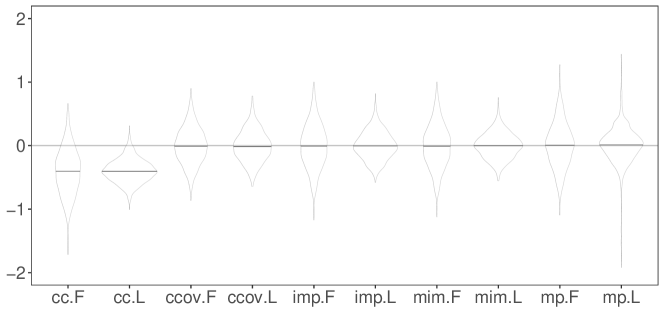
(ii) Scenario (ii) with $N=500$

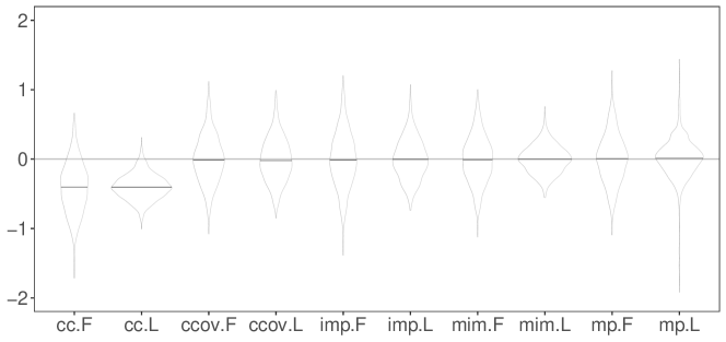
(iii) Scenario (iii) with $N=10,000$

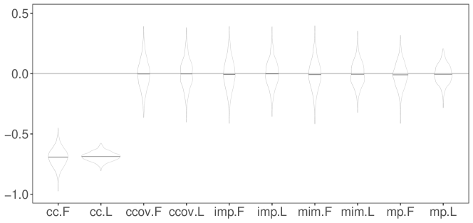
Application

Duflo et al. (2011) conducted a randomized field experiment in Western Kenya to study the effect of a time-limited utility cost reduction on fertilizer use. The experiment took place over two seasons from 2003 to 2005 after a series of small-scale pilot programs. We use their data from the first season to illustrate the methods for handling missing covariates.

The first season began after the 2003 short rain harvest to facilitate fertilizer purchase for the 2004 long rain season. The treatment was implemented in the form of free delivery of fertilizer as a time-limited reduction in the cost to acquiring fertilizer. One major outcome of interest is the fertilizer use in the first season after long rains 2004. Farmers were randomly assigned to receive either the treatment or control. A total of $N=877$ participant farmers were tracked for a follow-up usage survey, among which $N_{1}=204$ received the treatment and the rest $N_{0}=N-N_{1}=673$ received control. They constitute the study population of the original analysis reported by Duflo et al. (2011).

We follow Duflo et al. (2011) to consider $J=27$ covariates, including educational attainment, previous fertilizer usage, gender, income, whether the farmer’s home has mud walls, a mud floor, or a thatch roof, and whether the farmer has received a starter kit in the past. A total of $N^{\textup{cc}}=716$ farmers have all covariates observed, accounting for $81.64\%$ of the study population. Missingness of covariates happens in 7 out of the $J=27$ covariates with a total of 9 missing patterns summarized in Table 2.

Table 2: Counts of the nine missingness patterns for the incomplete covariates

missingness pattern	count
0000000	716
0000100	59
0001000	1
0010011	2
0100000	19
0100100	1
1000000	1
1011111	71
1111111	7

Table 3 summarizes the results from our re-analysis of the data. We exclude the missingness-pattern method from the comparison due to the small sizes of 4 missingness-pattern strata with $N_{(m)}<5$. The remaining four strategies return coherent results about a significant and fairly sizable effect of cost reduction on fertilizer use. The complete-case analysis with Fisher (1935)’s specification corresponds to the original analysis in Duflo et al. (2011), and yields the largest point estimate, 0.144, overall. This, together with the also large result from Lin (2013)’s model, 0.135, suggests the possibility of $\tau^{\textup{cc}}>\tau$ in the study population. The complete-covariate analysis, on the other hand, yields the most conservative $p$-values, which is coherent with our theory.

Table 3: Re-analysis of the data from Duflo et al. (2011). For comparison, $\hat{\tau}_{\textsc{n}}=0.112$ and $\hat{\text{se}}_{\textsc{n}}=0.039$ with $p$-value $=0.004$. We exclude the missingness-pattern method.

	$\hat{\tau}_{\textsc{f}}^{\dagger}$			$\hat{\tau}_{\textsc{l}}^{\dagger}$
strategy	estimate	robust s.e.	$p$-value	estimate	robust s.e.	$p$-value
cc	0.144	0.04	0	0.135	0.041	0.001
ccov	0.106	0.038	0.006	0.096	0.038	0.012
imp	0.129	0.037	0	0.123	0.037	0.001
mim	0.132	0.037	0	0.119	0.037	0.001

Extensions

7.1 Other regression specifications

Recall the hierarchy of model parsimony from Section 4.6. The missingness-pattern method gives the most saturated model under the fully interacted aggregate specification (16), and has the complete-covariate analysis, single imputation, and the missingness-indicator method all as its restricted variants. An immediate implication is that any subset of $u_{i}^{\textup{mp}}(c)$, up to a non-degenerate linear transformation, affords a valid covariate vector to form the additive and fully interacted regressions when simplifications are needed. This implies a whole spectrum of possible restrictions on (16) depending on the nature of the data. We illustrate below two types of restrictions of possible theoretical and practical interests.

The first type of restrictions are large-sample inference oriented, and focus on trade-offs between the missingness-indicator method and the missingness pattern method when the former alone is inadequate for attaining the desired asymptotic efficiency. In cases where evidence suggests the covariates and missingness indicators affect the treatment effects interactively, an intuitive trade-off between the missingness-indicator method and the missingness-pattern method would be to use $x_{i}^{0}$, $M_{i}$, and all second-order interactions between $\{x_{i}^{0},M_{ij}:j=1,\ldots,J\}$, namely terms like $x_{i}^{0}M_{ij}$ and $M_{ij}M_{ij^{\prime}}$ for all $j\neq j^{\prime}\in\overline{\mathcal{J}}$, to form the covariate vector. The resulting estimator has higher asymptotic efficiency than $\hat{\tau}_{\textsc{l}}^{\textup{mim}}$ under the fully interacted specification.

The second type of restrictions are finite-sample inference oriented, and focus on trade-offs between the missingness-indicator method and single imputation when the former is subject to considerable finite-sample bias. In particular, the missingness-indicator method involves $(4J+2)$ coefficients under the fully interacted specification (8), and can be demanding on sample sizes when $J$ is large. In cases where this results in large finite-sample variations, an alternative is to include only a subset of $M_{i}$ with the highest partial $R^{2}$ in forming the covariate vector. Alternatively, we could define $J_{i}=\sum_{j=1}^{J}(1-M_{ij})$ as the count of observed entries for unit $i$, and form the additive and fully interacted regressions based on the missingness-count covariate $x_{i}^{\textup{mc}}(c)=(\{x_{i}^{\textup{imp}}(c)\}^{\mathrm{\scriptscriptstyle T}},J_{i})^{\mathrm{\scriptscriptstyle T}}\in\mathbb{R}^{J+1}$. This idea of augmenting the covariates with $J_{i}$ was first proposed by Rummel (1970) in the context of factor analysis, and can be easily adapted for the current setting of multiple regression model; see Anderson et al. (1983) for a review. In addition, recall $C_{i}$ as the complete-case indicator for unit $i$. We could also augment $x_{i}^{\textup{imp}}(c)$ with $C_{i}$ and form the additive and fully interacted regressions using $x_{i}^{\textup{cim}}(c)=(\{x_{i}^{\textup{imp}}(c)\}^{\mathrm{\scriptscriptstyle T}},C_{i})^{\mathrm{\scriptscriptstyle T}}$. This gives us three ways to include the missingness information with less covariates than $x_{i}^{\textup{mim}}(c)$. A caveat is that the minimum specification that ensures invariance to $c$ must include all missingness indicators in ols. The three restricted variants thus improve the finite-sample performances at the cost of losing the numerical invariance.

Eventually, the choice of restrictions can be based on the data, and thus necessarily involves a model-selection step. Analyzing this type of procedure is non-trivial for design-based inference. Bloniarz et al. (2016) started the literature by augmenting Lin (2013)’s method with a lasso step for variable selection. We can also augment the fully-interacted ols for the missingness-pattern method with a lasso step. However, deriving its theoretical properties is a challenging research question. We leave the detailed theory to future work.

7.2 Cluster randomization

Consider $N$ units nested in $I$ clusters of sizes $n_{i}\ (i=1,\ldots,I;\ \sum_{i=1}^{I}n_{i}=N)$. Cluster randomization randomly assigns $I_{1}$ clusters to receive the treatment and the rest $I_{0}=I-I_{1}$ clusters to receive the control. We use $i$ to index the clusters as the randomization units and, with a slight abuse of notation, use $I$ to denote the cluster number when there is no confusion with the identity matrix.

Let $\{Y_{il}(z):z=0,1\}$ be the potential outcomes for the $l$th unit in cluster $i$, also referred to as unit $il\ (i=1,\ldots,I;\ l=1,\ldots,n_{i})$. The finite-population average treatment effect equals $\tau=N^{-1}\sum_{i=1}^{I}\sum_{l=1}^{n_{i}}\{Y_{il}(1)-Y_{il}(0)\}$. Let $Z_{i}$ be the treatment level received by cluster $i$. The observed outcome for unit $il$ is $Y_{il}=Z_{i}Y_{il}(1)+(1-Z_{i})Y_{il}(0)$. We further observe a $J$-dimensional covariate vector $x_{il}=(x_{il,1},\ldots,x_{il,J})^{\mathrm{\scriptscriptstyle T}}$ for each unit with $\bar{x}=N^{-1}\sum_{i=1}^{I}\sum_{l=1}^{n_{i}}x_{il}$. Regressions

$$Y_{il}\sim 1+Z_{i}+x_{il},$$ (18)

$$Y_{il}\sim 1+Z_{i}+(x_{il}-\bar{x})+Z_{i}(x_{il}-\bar{x})$$

over $i=1,\ldots,I;\ l=1,\ldots,n_{i}$ afford two intuitive specifications to estimate $\tau$ as the coefficients of $Z_{i}$. In fact, they are identical to the specifications under complete randomization with the individual-level treatment indicators, denoted by $Z_{il}$ for unit $il$, satisfying $Z_{il}=Z_{i}$ under cluster randomization. Su and Ding (2021) showed the validity of the resulting regression estimators and their associated cluster-robust standard errors for large-sample Wald-type inferences.

In the case where the $x_{il}$’s are only partially observed, all five strategies for handling missingness under complete randomization extend to the current setting with no need of modification. Assume the missingness is unaffected by the treatment assignment. We can derive results in parallel with Propositions 1–7 by assuming the corresponding regularity conditions for cluster randomization. In particular, let $M_{il}$ be the vector of missingness indicators for unit $il$, and $x_{il}^{0}$ be the imputed covariates with all missing values filled with 0. Replacing $x_{il}$ by $x_{il}^{\textup{mim}}=((x^{0}_{il})^{\mathrm{\scriptscriptstyle T}},M_{il}^{\mathrm{\scriptscriptstyle T}})^{\mathrm{\scriptscriptstyle T}}$ in (18) yields Lin (2013)’s estimator under the missingness-indicator method.

Whereas the above approach works for both complete and cluster randomizations with identical regression specifications, the peculiarity of cluster randomization allows us to also form regressions based on cluster total data. In particular, let $\bar{n}=N/I$ be the average cluster size, and let $\tilde{Y}_{i\cdot}(z)=\bar{n}^{-1}\sum_{l=1}^{n_{i}}Y_{il}(z)$, $\tilde{Y}_{i\cdot}=\bar{n}^{-1}\sum_{l=1}^{n_{i}}Y_{il}$, and $\tilde{x}_{i\cdot}=\bar{n}^{-1}\sum_{l=1}^{n_{i}}x_{il}$ be the cluster totals of potential outcomes, observed outcomes, and covariates scaled by $\bar{n}$. Then $\tilde{Y}_{i\cdot}=Z_{i}\tilde{Y}_{i\cdot}(1)+(1-Z_{i})\tilde{Y}_{i\cdot}(0)$ gives the observed analog of $\tilde{Y}_{i\cdot}(z)$. This, together with $\tau=I^{-1}\sum_{i=1}^{I}\{\tilde{Y}_{i\cdot}(1)-\tilde{Y}_{i\cdot}(0)\},$ ensures that $(Z_{i},\tilde{Y}_{i\cdot})_{i=1}^{I}$ is equivalent to the observed data from a complete randomization with potential outcomes $\{\tilde{Y}_{i\cdot}(0),\tilde{Y}_{i\cdot}(1)\}_{i=1}^{I}$ and average treatment effect $\tau$ (Middleton and Aronow 2015; Li and Ding 2017). The coefficient of $Z_{i}$ from the cluster-level regression $\tilde{Y}_{i\cdot}\sim 1+Z_{i}$ coincides with the difference in means of the $\tilde{Y}_{i\cdot}$’s and affords an unbiased estimator of $\tau$. Su and Ding (2021) showed that applying Lin (2013)’s estimator with scaled cluster totals further improves efficiency, and more importantly, asymptotically dominates the estimators from individual-level regressions (18) and (18). With missing covariates, we first impute all missing covariates with zero, denoted by $x^{0}_{il}$ for unit $il$, and define the cluster-level covariate vector as $u_{i}^{\textup{mim}}=(n_{i},(\tilde{x}^{0}_{i\cdot})^{\mathrm{\scriptscriptstyle T}},\tilde{M}_{i\cdot}^{\mathrm{\scriptscriptstyle T}})^{\mathrm{\scriptscriptstyle T}}$ where $\tilde{M}_{i\cdot}=\bar{n}^{-1}\sum_{l=1}^{n_{i}}M_{il}$ and $\tilde{x}^{0}_{i\cdot}=\bar{n}^{-1}\sum_{l=1}^{n_{i}}x_{il}^{0}$. Let $\bar{u}^{\textup{mim}}=I^{-1}\sum_{i=1}^{I}u_{i}^{\textup{mim}}$ be the average of $u_{i}^{\textup{mim}}$’s over the $I$ clusters. Extending Su and Ding (2021) to the case with missing covariates yields regression

$$\tilde{Y}_{i\cdot}\sim 1+Z_{i}+(u_{i}^{\textup{mim}}-\bar{u}^{\textup{mim}})+Z_{i}(u_{i}^{\textup{mim}}-\bar{u}^{\textup{mim}})$$

over $i=1,\ldots,I$. The resulting estimator ensures higher asymptotic efficiency than that from (18). It is our final recommendation.

7.3 Stratified randomization

Given a study population nested in $K$ strata, indexed by $k=1,\ldots,K$, stratified randomization conducts an independent complete randomization in each stratum (Miratrix et al. 2013; Liu and Yang 2020). Let $\omega_{[k]}$ be the proportion of units and $\tau_{[k]}$ be the average treatment effect within stratum $k$ $(k=1,\ldots,K)$. The finite-population average treatment effect equals $\tau=\sum_{k=1}^{K}\omega_{[k]}\tau_{[k]}$. In the case where the covariates are partially observed, we can form $\hat{\tau}^{\dagger}_{{\star}[k]}$ and $\hat{\text{se}}_{{\star}[k]}^{\dagger}$ as the basic estimator and robust standard error within each stratum $k$ for $\dagger\in\{\textup{cc},\textup{ccov},\textup{imp},\textup{mim},\textup{mp}\}$ and ${\star}={\textsc{f}},{\textsc{l}}$, and use their respective weighted averages, namely $\hat{\tau}_{{\star}}^{\dagger}=\sum_{k=1}^{K}\omega_{[k]}\hat{\tau}_{{\star}[k]}^{\dagger}$ and $(\hat{\text{se}}^{\dagger}_{\star})^{2}=\sum_{k=1}^{K}\omega_{[k]}^{2}(\hat{\text{se}}^{\dagger}_{{\star}[k]})^{2}$, as our point estimator and the corresponding squared robust standard error. We can derive results in parallel with Propositions 1–7 by assuming the corresponding regularity conditions hold within all strata.

7.4 Missingness that depends on the treatment assignment

The discussion so far requires Condition 2 with the missingness unaffected by the treatment assignment, that is, $M_{i}(0)=M_{i}(1)=M_{i}$ for all $i=1,\ldots,N$. The resulting missingness indicators are effectively fully observed covariates. Without Condition 2, $M_{i}=M_{i}(0)+Z_{i}\{M_{i}(1)-M_{i}(0)\}$ takes different values under different realized values of $Z_{i}$. A direct implication is that the vectors of $x_{i}^{\dagger}$’s that we use to form the additive and fully interacted regressions for $\dagger\in\{\textup{cc},\textup{ccov},\textup{imp},\textup{mim},\textup{mp}\}$ can no longer be seen as standard covariates unaffected by the treatment even asymptotically, imposing additional complications for quantifying the design-based properties of the resulting estimators.

As it turns out, among the estimators in Table 1, only $\hat{\tau}_{\star}^{\textup{ccov}}\ ({\star}={\textsc{f}},{\textsc{l}})$ from the complete-covariate analysis remain consistent without Condition 2. It is thus our recommendation in the absence of Condition 2. Recall from Proposition 7 that under Condition 2, $\hat{\tau}_{\textsc{l}}^{\textup{ccov}}$ has the largest asymptotic variance among the consistent $\hat{\tau}_{\textsc{l}}^{\dagger}$’s. Its consistency in the absence of Condition 2 thus gives an analog of the bias-variance trade-off in terms of the asymptotic biases and variances. We formalize the results in the Supplementary Material.

Discussion

We proposed to use Lin (2013)’s model to adjust for missing covariates in randomized experiments by imputing missing covariates with zeros and augmenting the covariates with missingness indicators. When the treatment does not affect the missingness indicators, this missingness-indicator method is consistent for the average treatment effect and more efficient than the unadjusted estimator, the complete-covariate analysis, and the estimators based on imputed covariates alone. It can be conveniently implemented via ols. We also proposed the missingness-pattern method as a modification to reap additional asymptotic efficiency.

We focused on constructing large-sample Wald-type confidence intervals based on consistent point estimators and conservative standard errors. Building upon these results, it is immediate to extend Zhao and Ding (2021) to construct robust Fisher randomization tests adjusting for covariates subject to missingness. In particular, using a studentized statistic based on any consistent estimator and the associated conservative standard error in the Fisher randomization test yields a $p$-value that is finite-sample exact under the strong null hypothesis $\tau_{i}=0$ for all $i$ and asymptotically conservative under the weak null hypothesis $\tau=0$. By duality, this also gives a confidence interval by inverting a sequence of Fisher randomization tests.

As an alternative to regression, weighting based on the propensity score is another simple yet powerful method to improve efficiency in randomized experiments. Shen et al. (2014) and Zeng et al. (2021) have shown that regression and weighting are equivalent asymptotically. With missing covariates, one option is to use the generalized propensity score (Rosenbaum and Rubin 1984) to construct weighting estimators. We conjecture that the equivalence between regression and weighting also holds even with missing covariates, but leave the theoretical analysis to future work.

Section S1 gives the more general results under possible violations of Condition 2.

Section S2 reviews the key lemmas.

Sections S3–S5 give the proofs of the results in the main text and Section S1 under individual strategies. The proofs for the complete-covariate analysis are short and given in the text. We verify the general results without Condition 2 unless specified otherwise.

Notation

Consider an experiment with two treatment levels, $\mathcal{T}=\{0,1\}$, and a finite population of size $N$. Given $\{u_{i}(z),v_{i}(z):z\in\mathcal{T};\ i=1,\ldots,N\}$, where $u_{i}(z)$ and $v_{i}(z)$ are two arbitrary potential outcome vectors for unit $i$, let $\bar{u}(z)=N^{-1}\sum_{i=1}^{N}u_{i}(z)$, $\bar{v}(z)=N^{-1}\sum_{i=1}^{N}v_{i}(z)$, and $S_{u(z),v(z^{\prime})}=N^{-1}\sum_{i=1}^{N}\{u_{i}(z)-\bar{u}(z)\}\{v_{i}(z^{\prime})-\bar{v}(z^{\prime})\}^{\mathrm{\scriptscriptstyle T}}$ be the finite-population means and covariances, respectively, for $z,z^{\prime}\in\mathcal{T}$. We use $N$ instead of $(N-1)$ as the divisors for the covariances; the simplification does not affect the validity of the proofs with $(N-1)/N=1+o(1)$ as $N\to\infty$. Abbreviate $u_{i}(z)$, $\bar{u}(z)$, and $S_{u(z),v(z^{\prime})}$ to $u_{i}$, $\bar{u}$, and $S_{u,v(z^{\prime})}$, respectively, if $u_{i}(z)$ is unaffected by the treatment with $u_{i}(0)=u_{i}(1)$ for all $i$. Abbreviate $S_{u(z),v(z)}$ as $S_{uv}(z)$ occasionally to simplify the notation.

Further let $Z_{i}\in\mathcal{T}$ be the treatment indicator of unit $i$. The observed values of $u_{i}(z)$ and $v_{i}(z)$ are $u_{i}=Z_{i}u_{i}(1)+(1-Z_{i})u_{i}(0)$ and $v_{i}=Z_{i}v_{i}(1)+(1-Z_{i})v_{i}(0)$ for unit $i$. Let $N_{z}=\sum_{i=1}^{N}1(Z_{i}=z)$ be the number of units under treatment $z$. Let $\hat{u}(z)=N_{z}^{-1}\sum_{i:Z_{i}=z}u_{i}$, $\hat{v}(z)=N_{z}^{-1}\sum_{i:Z_{i}=z}v_{i}$, and $\hat{S}_{uv}(z)=N_{z}^{-1}\sum_{i:Z_{i}=z}\{u_{i}-\hat{u}(z)\}\{v_{i}-\hat{v}(z)\}^{\mathrm{\scriptscriptstyle T}}$ be the sample analogs of $\bar{u}(z)$, $\bar{v}(z)$, and $S_{u(z),v(z)}$, respectively, for units under treatment $z$. We use $N_{z}$ instead of $(N_{z}-1)$ as the divisors for the sample covariances; the simplification does not affect the validity of the proofs with $(N_{z}-1)/N_{z}=1+o(1)$ as $N\to\infty$ and $e_{z}=N_{z}/N$ converges to a limit in $(0,1)$.

Write $a_{N}\overset{.}{\sim}b_{N}$ if $\sqrt{N}(a_{N}-b_{N})={o_{P}(1)}$ for sequences of random variables $(a_{N})_{N=1}^{\infty}$ and $(b_{N})_{N=1}^{\infty}$. Slutsky’s theorem ensures that $\sqrt{N}a_{N}$ and $\sqrt{N}b_{N}$ have the same limiting distribution as long as $a_{N}\overset{.}{\sim}b_{N}$ and either $(\sqrt{N}a_{N})_{N=1}^{\infty}$ or $(\sqrt{N}b_{N})_{N=1}^{\infty}$ has a limiting distribution. We suppress the subscript $N$ when no confusion would arise.

Let $\circ$ denote the Hadamard product and $\otimes$ denote the Kronecker product of matrices, respectively. We will repeatedly use the following property of the Kronecker product:

$$(H_{1}H_{2})\otimes(H_{3}H_{4})=(H_{1}\otimes H_{3})(H_{2}\otimes H_{4})$$

for matrices $H_{k}\ (k=1,2,3,4)$ with compatible dimensions.

Extensions to missingness that depends on the assignment

We first introduce the notation without Condition 2. Recall $M_{i}=(M_{i1},\ldots,M_{iJ})^{\mathrm{\scriptscriptstyle T}}$ as the observed missingness indicators of unit $i$ with $M_{ij}=1(\text{$x_{ij}$ is missing})$. Recall $M_{i}(z)=(M_{i1}(z),\ldots,M_{iJ}(z))^{\mathrm{\scriptscriptstyle T}}$ as the potential value of $M_{i}$ if unit $i$ were assigned to treatment $z$. For $C_{i}=1(M_{i}=0_{J})$ and $A_{i}=1_{J}-M_{i}$, let $C_{i}(z)=1\{M_{i}(z)=0_{J}\}$ and $A_{i}(z)=(A_{i1}(z),\ldots,A_{iJ}(z))^{\mathrm{\scriptscriptstyle T}}=1_{J}-M_{i}(z)$ be the corresponding potential values, respectively. Let $x_{i}^{0}(z)=A_{i}(z)\circ x_{i}=(A_{i1}(z)x_{i1},\ldots,A_{iJ}(z)x_{iJ})^{\mathrm{\scriptscriptstyle T}}$ be the corresponding imputed variant of $x_{i}$ with all missing elements replaced by 0. Condition S1 generalizes Condition 3 to possible violations of Condition 2.

Condition S1.

As $N\to\infty$, (i) $e_{z}$ has a limit in $(0,1)$ for $z=0,1$; (ii) the first two moments of $\{Y_{i}(z),x_{i},M_{i}(z),C_{i}(z),C_{i}(z)Y_{i}(z),C_{i}(z)x_{i},A_{i}(z)\circ x_{i}:z=0,1\}_{i=1}^{N}$ have finite limits, and (iii) there exists a $u_{0}<\infty$ independent of $N$ such that $N^{-1}\sum_{i=1}^{N}\|x_{i}\|_{4}^{4}\leq u_{0}$ and $N^{-1}\sum_{i=1}^{N}Y_{i}^{4}(z)\leq u_{0}$ for $z=0,1$.

Let $\bar{M}(z)$, $\bar{C}(z)$, and $\overline{Ax}(z)$ denote the averages of $M_{i}(z)$, $C_{i}(z)$, and $A_{i}(z)\circ x_{i}$ over $i=1,\ldots,N$, respectively. Let $\hat{M}(z)$, $\hat{C}(z)$, and $\widehat{Ax}(z)$ be the corresponding sample analogs over units under treatment $z$.

S1.1 Complete-case analysis

Refer to $\{i:C_{i}(z)=1\}$ as the $z$-complete cases with all covariates observed if assigned to treatment $z$. Refer to $\{i:C_{i}=1\}$ as the observed complete cases with all covariates observed under the realized assignment. The two sets of units coincide under Condition 2. Analogous to the definitions of $N^{\textup{cc}}$, $\bar{Y}^{\textup{cc}}(z)$, $\bar{x}^{\textup{cc}}$, $S_{xx}^{\textup{cc}}$, and $\tau^{\textup{cc}}$ over the observed complete cases from the main text, let $N^{\textup{cc}}(z)=\sum_{i=1}^{N}C_{i}(z)$ be the number of the $z$-complete cases, with $\bar{C}(z)=N^{-1}\sum_{i=1}^{N}C_{i}(z)=N^{\textup{cc}}(z)/N$ as the corresponding proportion; let $\bar{Y}^{\textup{cc}}(z)$, $\bar{x}^{\textup{cc}}(z)$, $S_{xx}^{\textup{cc}}(z)$, and $S_{xY}^{\textup{cc}}(z)$ be the corresponding finite-population means and covariances of $Y_{i}(z)$’s and $x_{i}$’s over $\{i:C_{i}(z)=1\}$; and let $\tau^{\textup{cc}}=\bar{Y}^{\textup{cc}}(1)-\bar{Y}^{\textup{cc}}(0)$. With $C_{i}(0)$ and $C_{i}(1)$ no longer necessarily equal under possible violations of Condition 2, $\bar{Y}^{\textup{cc}}(0)$ and $\bar{Y}^{\textup{cc}}(1)$ are now the average potential outcomes over two distinct subsets of units, namely $\{i:C_{i}(0)=1\}$ and $\{i:C_{i}(1)=1\}$, such that the resulting difference $\tau^{\textup{cc}}$ is no longer necessarily a causal effect. Let

$$\rho_{z}^{\textup{cc}}=\frac{e_{z}\bar{C}(z)}{e_{1}\bar{C}(1)+e_{0}\bar{C}(0)}\qquad\text{for}\quad z=0,1$$

with $\rho_{0}^{\textup{cc}}+\rho_{1}^{\textup{cc}}=1$. As $N\to\infty$, $\rho_{z}^{\textup{cc}}$ gives the probability limit of the proportion of observed complete cases that receive treatment $z$; we give the details in Lemma S5. Let $\bar{Y}^{\textup{ic}}(z)$ be the average of $Y_{i}(z)$’s over the $z$-incomplete cases, $\{i:C_{i}(z)=0\}$, analogous to $\bar{Y}^{\textup{cc}}(z)$.

We can show that $\bar{Y}^{\textup{cc}}(z)$, $\bar{x}^{\textup{cc}}(z)$, $S_{xx}^{\textup{cc}}(z)$, $S_{xY}^{\textup{cc}}(z)$, $\tau^{\textup{cc}}$, $\rho_{z}^{\textup{cc}}$, and $\bar{Y}^{\textup{ic}}(z)$ all have finite limits under Condition S1. We also use the same symbols to denote their respective limits when no confusion would arise.

Proposition S1.

Assume complete randomization, Condition S1, and the limits of $\{S_{xx}^{\textup{cc}}(z):z=0,1\}$ are both positive definite. We have

$$\hat{\tau}_{\star}^{\textup{cc}}-\tau=(\tau^{\textup{cc}}-\tau)-\{\bar{x}^{\textup{cc}}(1)-\bar{x}^{\textup{cc}}(0)\}^{\mathrm{\scriptscriptstyle T}}\gamma_{{\star}}^{\textup{cc}}+{o_{P}(1)}\qquad\text{for}\quad{\star}={\textsc{f}},{\textsc{l}},$$

where $\gamma_{\textsc{f}}^{\textup{cc}}=\{\rho_{0}^{\textup{cc}}S_{xx}^{\textup{cc}}(0)+\rho_{1}^{\textup{cc}}S_{xx}^{\textup{cc}}(1)\}^{-1}\{\rho_{0}^{\textup{cc}}S_{xY}^{\textup{cc}}(0)+\rho_{1}^{\textup{cc}}S_{xY}^{\textup{cc}}(1)\}$, and $\gamma_{{\textsc{l}}}^{\textup{cc}}=\rho_{0}^{\textup{cc}}\gamma_{{\textsc{l}},1}^{\textup{cc}}+\rho_{1}^{\textup{cc}}\gamma_{{\textsc{l}},0}^{\textup{cc}}$ with $\gamma_{{\textsc{l}},z}^{\textup{cc}}=\{S_{xx}^{\textup{cc}}(z)\}^{-1}S_{xY}^{\textup{cc}}(z)$ for $z=0,1$. A sufficient and necessary conditions for $\tau^{\textup{cc}}=\tau$ is $\{1-\bar{C}(1)\}\{\bar{Y}^{\textup{cc}}(1)-\bar{Y}^{\textup{ic}}(1)\}=\{1-\bar{C}(0)\}\{\bar{Y}^{\textup{cc}}(0)-\bar{Y}^{\textup{ic}}(0)\}$.

With $\bar{x}^{\textup{cc}}(1)$ and $\bar{x}^{\textup{cc}}(0)$ no longer necessarily equal in the absence of Condition 2, Proposition S1 generalizes Proposition 1 to possible violations of Condition 2, and illustrates the additional source of asymptotic bias, in addition to the difference between $\tau^{\textup{cc}}$ and $\tau$, due to the possible difference between $\bar{x}^{\textup{cc}}(1)$ and $\bar{x}^{\textup{cc}}(0)$.

S1.2 Complete-covariate analysis

Condition S2.

The set of observed complete covariates $\mathcal{J}=\{j:M_{ij}(Z_{i})=0\text{ for all }i=1,\ldots,N\}$ remains unchanged over all possible values of $(Z_{i})_{i=1}^{N}$ under complete randomization for $N=1,\ldots,\infty$, with $S_{xx}^{\textup{ccov}}$ and its limit under Condition S1 both being positive definite as $N\to\infty$.

Proposition S2.

Assume complete randomization and Conditions S1–S2. Proposition 2 holds regardless of whether Condition 2 holds or not.

Echoing the comments under Proposition 2, Condition S2 ensures that the set $\mathcal{J}$ remains constant over all possible treatment assignments, rendering $x_{i}^{\textup{ccov}}$ an effective true covariate vector unaffected by the randomization. The result of Proposition S2 follows from applying Lemma 1 to the finite population of $\{Y_{i}(0),Y_{i}(1),x_{i}^{\textup{ccov}}\}_{i=1}^{N}$ regardless of whether Condition 2 holds or not, and justifies the large-sample Wald-type inference based on $(\hat{\tau}_{\star}^{\textup{ccov}},\hat{\text{se}}_{\star}^{\textup{ccov}})$.

S1.3 Single imputation and missingness-indicator method

Recall $x^{\textup{imp}}_{i}(c)=(x^{\textup{imp}}_{i1}(c_{1}),\ldots,x^{\textup{imp}}_{iJ}(c_{J}))^{\mathrm{\scriptscriptstyle T}}$ as the imputed covariate vector with $x_{ij}^{\textup{imp}}(c_{j})=(1-M_{ij})x_{ij}+M_{ij}c_{j}$. Single imputation uses $x^{\textup{imp}}_{i}(c)$ to form the additive and fully interacted regressions as (5) and (6). The missingness-indicator method uses $x_{i}^{\textup{mim}}(c)=(x^{\textup{imp}}_{i}(c)^{\mathrm{\scriptscriptstyle T}},M_{i}^{\mathrm{\scriptscriptstyle T}})^{\mathrm{\scriptscriptstyle T}}$ to form the additive and fully interacted regressions as (7) and (8).

Let $x^{\textup{imp}}_{ij}(z;c_{j})=\{1-M_{ij}(z)\}x_{ij}+M_{ij}(z)c_{j}$ be the potential value of $x^{\textup{imp}}_{ij}(c_{j})$ if unit $i$ were assigned to treatment $z$; we treat $c_{j}$ as fixed in defining $x^{\textup{imp}}_{ij}(z;c_{j})$ despite its possible dependence on $(Z_{i})_{i=1}^{N}$. Let $x^{\textup{imp}}_{i}(z;c)=\{x_{ij}^{\textup{imp}}(z;c_{j})\}_{j=1}^{J}$ and $x_{i}^{\textup{mim}}(z;c)=(x_{i}^{\textup{imp}}(z;c)^{\mathrm{\scriptscriptstyle T}},M_{i}(z)^{\mathrm{\scriptscriptstyle T}})^{\mathrm{\scriptscriptstyle T}}$ be the corresponding potential values of $x^{\textup{imp}}_{i}(c)$ and $x_{i}^{\textup{mim}}(c)$, respectively. We focus on imputations $c=(c_{j})_{j=1}^{J}$ with finite probability limits $c_{\infty}=(c_{j,\infty})_{j=1}^{J}$:

$$\mathcal{C}^{\prime}=\{c\in\mathbb{R}^{J}:\operatorname*{plim}c_{j}=c_{j,\infty}<\infty\ (j=1,\ldots,J)\text{ under complete randomization and Condition \ref{asym}}\}.$$

In particular, $\mathcal{C}^{\prime}$ generalizes the definition of $\mathcal{C}$ in the main text to possible violations of Condition 2. The constant imputation with $c_{j}=0$ is a special case of $c\in\mathcal{C}^{\prime}$ with $c_{\infty}=0_{J}$; the unconditional mean imputation with $c_{j}=\hat{x}_{j}^{\rm obs}$ is also a special case with $c_{j,\infty}=\{e_{1}\bar{A}_{j}(1)+e_{0}\bar{A}_{j}(0)\}^{-1}\{e_{1}\overline{Ax}_{j}(1)+e_{0}\overline{Ax}_{j}(0)\}$, where $\bar{A}_{j}(z)=N^{-1}\sum_{i=1}^{N}A_{ij}(z)$ and $\overline{Ax}_{j}(z)=N^{-1}\sum_{i=1}^{N}A_{ij}(z)x_{ij}$ denote the $j$th elements of $\bar{A}(z)$ and $\overline{Ax}(z)$, respectively.

Let $S_{xx}^{\dagger}(z;c)$ and $S_{xY}^{\dagger}(z;c)$ be the finite-population covariances of $\{x_{i}^{\dagger}(z;c)\}_{i=1}^{N}$ and $\{x_{i}^{\dagger}(z;c),Y_{i}(z)\}_{i=1}^{N}$ for $\dagger\in\{\textup{imp},\textup{mim}\}$. For $c\in\mathcal{C}^{\prime}$ with $\operatorname*{plim}c=c_{\infty}$, we can show that $S_{xx}^{\dagger}(z;c_{\infty})$ and $S_{xY}^{\dagger}(z;c_{\infty})$ have finite limits under Condition S1 for all $z=0,1$ and $\dagger\in\{\textup{imp},\textup{mim}\}$. We will use $S_{xx}^{\dagger}(z;c_{\infty})$ and $S_{xY}^{\dagger}(z;c_{\infty})$ to also denote their respective limiting values when no confusion would arise. Let $D_{c,\infty}=\operatorname{diag}(c_{j,\infty})_{j=1}^{J}$ be the $J\times J$ diagonal matrix.

Recall $\hat{\tau}_{\star}^{\textup{mim}}=\hat{\tau}_{\star}^{\textup{mim}}(0_{J})$ as the value of $\hat{\tau}_{\star}^{\textup{mim}}(c)$ when we impute all missing covariates with 0. Lemma 3 holds without Condition 2 such that we still have $\hat{\tau}_{\star}^{\textup{mim}}(c)=\hat{\tau}_{\star}^{\textup{mim}}$ for all $c\in\mathbb{R}^{J}$.

Proposition S3.

Assume complete randomization, Condition S1, and $c\in\mathcal{C}^{\prime}$ with the limits of $S_{xx}^{\dagger}(z;c_{\infty})\ ({\dagger}=\textup{imp},\textup{mim};\ z=0,1)$ all being positive definite. We have

$$\hat{\tau}_{\star}^{\textup{imp}}(c)-\tau=-[\overline{Ax}(1)-\overline{Ax}(0)+D_{c,\infty}\{\bar{M}(1)-\bar{M}(0)\}]^{\mathrm{\scriptscriptstyle T}}\gamma_{{\star}}^{\textup{imp}}(c_{\infty})+{o_{P}(1)},$$

$$\hat{\tau}_{\star}^{\textup{mim}}(c)-\tau=-([\overline{Ax}(1)-\overline{Ax}(0)]^{\mathrm{\scriptscriptstyle T}},\ \{\bar{M}(1)-\bar{M}(0)\}^{\mathrm{\scriptscriptstyle T}})\gamma_{{\star}}^{\textup{mim}}(0_{J})+{o_{P}(1)}$$

for ${\star}={\textsc{f}},{\textsc{l}}$, where $\gamma_{{\textsc{f}}}^{\dagger}(c_{\infty})=\{e_{0}S_{xx}^{\dagger}(0;c_{\infty})+e_{1}S_{xx}^{\dagger}(1;c_{\infty})\}^{-1}\{e_{0}S_{xY}^{\dagger}(0;c_{\infty})+e_{1}S_{xY}^{\dagger}(1;c_{\infty})\}$ and $\gamma_{{\textsc{l}}}^{\dagger}(c_{\infty})=e_{0}\gamma_{{\textsc{l}},1}^{\dagger}(c_{\infty})+e_{1}\gamma_{{\textsc{l}},0}^{\dagger}(c_{\infty})$ with $\gamma_{{\textsc{l}},z}^{\dagger}(c_{\infty})=\{S_{xx}^{\dagger}(z;c_{\infty})\}^{-1}S_{xY}^{\dagger}(z;c_{\infty})$ for $\dagger\in\{\textup{imp},\textup{mim}\}$ and $z=0,1$.

With $\overline{Ax}(1)-\overline{Ax}(0)$ and $\bar{M}(1)-\bar{M}(0)$ no longer necessarily equal to $0_{J}$, Proposition S3 highlights the possible asymptotic biases of single imputation and the missingness-indicator method in the absence of Condition 2. We thus recommend using the complete-covariate analysis whenever the validity of Condition 2 is in doubt.

Whereas $\hat{\tau}_{\star}^{\textup{mim}}(c)$ is invariant to $c$ and thus precludes the possibility of bias reduction via crafted choice of $c$, the dependence of $\hat{\tau}_{\star}^{\textup{imp}}(c)$ on $c$ promises a way to reduce the asymptotic bias by a data-dependent choice of $c$. In particular, recall $\bar{A}_{j}(z)$ and $\overline{Ax}_{j}(z)$ as the $j$th elements of $\bar{A}(z)$ and $\overline{Ax}(z)$, respectively. A sufficient condition for $\hat{\tau}_{\star}^{\textup{imp}}(c)$ to be consistent is $\overline{Ax}(1)-\overline{Ax}(0)+D_{c,\infty}\{\bar{M}(1)-\bar{M}(0)\}=0_{J}$. Let $\hat{A}_{j}(z)=N_{z}^{-1}\sum_{i:Z_{i}=z}A_{ij}$ and $\widehat{Ax}_{j}(z)=N_{z}^{-1}\sum_{i:Z_{i}=z}A_{ij}x_{ij}$ be the sample analogs of $\bar{A}_{j}(z)$ and $\overline{Ax}_{j}(z)$, respectively. When $\bar{A}_{j}(0)\neq\bar{A}_{j}(1)$ for all $j$’s, we can choose

$$c_{j}=\frac{\widehat{Ax_{j}}(1)-\widehat{Ax_{j}}(0)}{\hat{A}_{j}(1)-\hat{A}_{j}(0)}\quad(j=1,\ldots,J)$$

to ensure

$$c_{j,\infty}=\frac{\overline{Ax}_{j}(1)-\overline{Ax}_{j}(0)}{\bar{A}_{j}(1)-\bar{A}_{j}(0)}\quad(j=1,\ldots,J)$$

to remove the asymptotic bias. When $\bar{A}_{j}(0)=\bar{A}_{j}(1)$ for some $j$’s, it is impossible to remove the bias by choosing the $c_{j}$’s.

S1.4 Missingness-pattern method

Recall that $\hat{\tau}_{\textsc{l}}^{\textup{mp}}$ equals the coefficient of $Z_{i}$ from the aggregate regression (16) for arbitrary $c\in\mathbb{R}^{J}$. Let $u_{i}^{\textup{mp}}=u_{i}^{\textup{mp}}(0_{J})$ be the value of $u_{i}^{\textup{mp}}(c)$ at $c=0_{J}$. Let $u_{i}^{\textup{mp}}(z)$ be the potential value of $u_{i}^{\textup{mp}}$ if unit $i$ were assigned to treatment $z$. It is the vector of $x_{i}^{\textup{imp}}(z;0_{J})$, $M_{i1}(z),\ldots,M_{iJ}(z)$, and all their interactions.

Let $\bar{u}^{\textup{mp}}(z)=N^{-1}\sum_{i=1}^{N}u_{i}^{\textup{mp}}(z)$ be the finite-population mean of $u_{i}^{\textup{mp}}(z)$ over $i=1,\ldots,N$. Let $S_{uu}^{\textup{mp}}(z)$ and $S_{uY}^{\textup{mp}}(z)$ be the finite-population covariances of $\{u_{i}^{\textup{mp}}(z)\}_{i=1}^{N}$ and $\{u_{i}^{\textup{mp}}(z),Y_{i}(z)\}_{i=1}^{N}$, respectively.

Condition S3.

As $N\to\infty$, for $z=0,1$, (i) $e_{z}$ has a limit between $(0,1)$, and (ii) $\bar{u}^{\textup{mp}}(z)$, $S_{uu}^{\textup{mp}}(z)$, and $S_{uY}^{\textup{mp}}(z)$ all have finite limits, with $S_{uu}^{\textup{mp}}(z)$ and its limit both being positive definite.

Proposition S4.

Assume complete randomization and Condition S3. We have

$$\hat{\tau}_{\textsc{l}}^{\textup{mp}}=\tau-\{\bar{u}^{\textup{mp}}(1)-\bar{u}^{\textup{mp}}(0)\}^{\mathrm{\scriptscriptstyle T}}\gamma_{\textsc{l}}^{\textup{mp}}+{o_{P}(1)},$$

where $\gamma_{\textsc{l}}^{\textup{mp}}=e_{1}^{-1}\gamma_{{\textsc{l}},0}^{\textup{mp}}+e_{0}^{-1}\gamma_{{\textsc{l}},1}^{\textup{mp}}$ with $\gamma_{{\textsc{l}},z}^{\textup{mp}}=\{S_{uu}^{\textup{mp}}(z)\}^{-1}S_{uY}^{\textup{mp}}(z)$ for $z=0,1$.

With $\bar{u}^{\textup{mp}}(0)$ and $\bar{u}^{\textup{mp}}(1)$ no longer necessarily equal, Proposition S3 highlights the possible asymptotic bias of $\hat{\tau}_{\textsc{l}}^{\textup{mp}}$ in the absence of Condition 2. The same result extends to $\hat{\tau}_{\textsc{f}}^{\textup{mp}}$ from the additive regressions as well. We relegate the details to Section S5.3.

Lemmas

Let $(Ax)_{i}(z)=A_{i}(z)\circ x_{i}$, $(CY)_{i}(z)=C_{i}(z)Y_{i}(z)$, and $(Cx)_{i}(z)=C_{i}(z)x_{i}$ be shorthand notations for $A_{i}(z)\circ x_{i}$, $C_{i}(z)Y_{i}(z)$, and $C_{i}(z)x_{i}$, respectively, with finite-population means $\overline{Ax}(z),\overline{CY}(z),$ and $\overline{Cx}(z)$ over $i=1,\ldots,N$. Let $(Ax)_{i}=A_{i}\circ x_{i}$, $(CY)_{i}=C_{i}Y_{i}$, and $(Cx)_{i}=C_{i}x_{i}$ be the observed values of $(Ax)_{i}(z)$, $(CY)_{i}(z)$, and $(Cx)_{i}(z)$, respectively, with $\widehat{Ax}(z),\widehat{CY}(z),$ and $\widehat{Cx}(z)$ as the sample analogs of $\overline{Ax}(z)$, $\overline{CY}(z)$, and $\overline{Cx}(z)$ over $\{i:Z_{i}=z\}$.

Lemma S1 gives the numerical expressions of $\hat{\tau}_{\star}\ ({\star}={\textsc{f}},{\textsc{l}})$. The result affords the basis for quantifying the sampling properties of $\hat{\tau}_{{\star}}^{\dagger}$’s for $\dagger\in\{\textup{cc},\textup{ccov},\textup{imp},\textup{mim},\textup{mp}\}$ and ${\star}={\textsc{f}},{\textsc{l}}$.

Lemma S1.

We have

$$\hat{\tau}_{\textsc{f}}=\hat{\tau}_{\textsc{n}}-\hat{\tau}_{x}^{\mathrm{\scriptscriptstyle T}}\hat{\gamma}_{\textsc{f}},$$

$$\hat{\tau}_{\textsc{l}}=\hat{\tau}_{\textsc{n}}-\hat{\tau}_{x}^{\mathrm{\scriptscriptstyle T}}\hat{\gamma}_{\textsc{l}}=\left[\hat{Y}(1)-\{\hat{x}(1)-\bar{x}\}^{\mathrm{\scriptscriptstyle T}}\hat{\gamma}_{{\textsc{l}},1}\right]-\left[\hat{Y}(0)-\{\hat{x}(0)-\bar{x}\}^{\mathrm{\scriptscriptstyle T}}\hat{\gamma}_{{\textsc{l}},0}\right],$$

where $\hat{\gamma}_{\textsc{f}}=\{e_{0}\hat{S}_{xx}(0)+e_{1}\hat{S}_{xx}(1)\}^{-1}\{e_{0}\hat{S}_{xY}(0)+e_{1}\hat{S}_{xY}(1)\}$ is the coefficient of $x_{i}$ from $Y_{i}\sim 1+Z_{i}+x_{i}$ over $i=1,\ldots,N$, and $\hat{\gamma}_{\textsc{l}}=e_{0}\hat{\gamma}_{{\textsc{l}},1}+e_{1}\hat{\gamma}_{{\textsc{l}},0}$ with $\hat{\gamma}_{{\textsc{l}},z}=\{\hat{S}_{xx}(z)\}^{-1}\hat{S}_{xY}(z)$ equaling the coefficient of $x_{i}$ from the treatment-specific ols fit $Y_{i}\sim 1+x_{i}$ over $\{i:Z_{i}=z\}$.

Proof of Lemma S1.

The numerical form of $\hat{\tau}_{\textsc{l}}$ follows from Zhao and Ding [2021, Proposition 1]. The numerical form of $\hat{\tau}_{\textsc{f}}$ follows from the basic properties of ols and, in particular, the Frisch–Waugh–Lovell theorem. ∎

Lemma S2 states the asymptotic normality of moment estimators under general complete randomization with $Q\geq 2$ treatment levels.

Lemma S2.

[Li and Ding, 2017, Theorems 3 and 5] In a completely randomized experiment with $N$ units and $Q$ treatment groups of sizes $(N_{q})_{q=1}^{Q}$, let $Y_{i}(q)$ be the $L$-dimensional potential outcome vector of unit $i$ under treatment $q$, and $S_{qq^{\prime}}=(N-1)^{-1}\sum_{i=1}^{N}\{Y_{i}(q)-\bar{Y}(q)\}\{Y_{i}(q^{\prime})-\bar{Y}(q^{\prime})\}^{\mathrm{\scriptscriptstyle T}}$ be the finite-population covariance. Let $\tau(\Gamma)=\sum_{q=1}^{Q}\Gamma_{q}\bar{Y}(q)$, where $\Gamma_{q}$ is an arbitrary $K\times L$ coefficient matrix for $q=1,\ldots,Q$. The estimator $\hat{\tau}(\Gamma)=\sum_{q=1}^{Q}\Gamma_{q}\hat{Y}(q)$ has mean $\tau(\Gamma)$ and covariance

$$\operatorname{cov}\{\hat{\tau}(\Gamma)\}=\sum_{q=1}^{Q}N_{q}^{-1}\Gamma_{q}S_{qq}\Gamma_{q}^{\mathrm{\scriptscriptstyle T}}-N^{-1}S_{\tau(\Gamma)}^{2},$$

where $S_{\tau(\Gamma)}^{2}$ is the finite-population covariance of $\{\tau_{i}(\Gamma)=\sum_{q=1}^{Q}\Gamma_{q}Y_{i}(q):\ i=1,\ldots,N\}$. If for any $1\leq q,q^{\prime}\leq Q$, $S_{qq^{\prime}}$ has a finite limit, $N_{q}/N$ has a limit in $(0,1)$, and $\max_{1\leq q\leq Q,1\leq i\leq N}\|Y_{i}(q)-\bar{Y}(q)\|^{2}_{2}/N\to 0$, then $N\operatorname{cov}\{\hat{\tau}(\Gamma)\}$ has a limiting value, denoted by $V$, and

$$\sqrt{N}\{\hat{\tau}(\Gamma)-\tau(\Gamma)\}\rightsquigarrow\mathcal{N}(0,V).$$

Lemma S3 follows from Lemma S2 and states the asymptotic joint normality of $\{\hat{C}(z),\widehat{CY}(z),\widehat{Cx}(z):z=0,1\}$ and that of $\{\hat{Y}(z),\hat{M}(z),\hat{C}(z),\widehat{Ax}(z):z=0,1\}$ without Condition 2. It affords the basis for verifying the asymptotic normality of $\hat{\tau}_{{\star}}^{\dagger}$’s.

Lemma S3.

Assume complete randomization and Condition S1. We have

$$\sqrt{N}\begin{pmatrix}\widehat{CY}(0)-\overline{CY}(0)\\ \widehat{CY}(1)-\overline{CY}(1)\\ \widehat{Cx}(0)-\overline{Cx}(0)\\ \widehat{Cx}(1)-\overline{Cx}(1)\\ \hat{C}(0)-\bar{C}(0)\\ \hat{C}(1)-\bar{C}(1)\end{pmatrix}\quad\text{and}\quad\sqrt{N}\begin{pmatrix}\hat{Y}(0)-\bar{Y}(0)\\ \hat{Y}(1)-\bar{Y}(1)\\ \widehat{Ax}(0)-\overline{Ax}(0)\\ \widehat{Ax}(1)-\overline{Ax}(1)\\ \hat{M}(0)-\bar{M}(0)\\ \hat{M}(1)-\bar{M}(1)\end{pmatrix}$$

are asymptotically normal with means $0_{4+2J}$ and $0_{4+4J}$, respectively.

Proof of Lemma S3.

We verify below the result for $\{\widehat{CY}(z),\widehat{Cx}(z),\hat{C}(z):z=0,1\}$. The proof for $\{\hat{Y}(z),\widehat{Ax}(z),\hat{M}(z):z=0,1\}$ is almost identical and thus omitted.

Let $G_{i}(z)=(C_{i}(z)Y_{i}(z),C_{i}(z)x_{i}^{\mathrm{\scriptscriptstyle T}},C_{i}(z))^{\mathrm{\scriptscriptstyle T}}$ be the augmented $(2+J)$-dimensional potential outcome vector of unit $i$. Condition S1 ensures that the finite-population covariance matrix of $\{G_{i}(0),G_{i}(1)\}_{i=1}^{N}$ has a finite limit, and it follows from

$$\|G_{i}(z)-\bar{G}(z)\|_{2}^{2} = \{C_{i}(z)Y_{i}(z)-\overline{CY}(z)\}^{2}+\|C_{i}(z)x_{i}-\overline{Cx}(z)\|_{2}^{2}+\{C_{i}(z)-\bar{C}(z)\}^{2}$$

$$\leq 2\{C_{i}(z)Y_{i}(z)\}^{2}+2\{\overline{CY}(z)\}^{2}+2\|C_{i}(z)x_{i}\|_{2}^{2}+2\|\overline{Cx}(z)\|_{2}^{2}+2\{C_{i}(z)\}^{2}+2\{\bar{C}(z)\}^{2}$$

$$\leq 2\{Y_{i}(z)\}^{2}+2\{\overline{CY}(z)\}^{2}+2\|x_{i}(z)\|_{2}^{2}+2\|\overline{Cx}(z)\|_{2}^{2}+2+2\{\bar{C}(z)\}^{2}$$

that $\max_{1\leq i\leq N;z=0,1}\|G_{i}(z)-\bar{G}(z)\|_{2}^{2}/N=o(1)$. The finite population of $\{G_{i}(0),G_{i}(1)\}_{i=1}^{N}$ thus satisfies the regularity conditions in Lemma S2, and ensures the joint asymptotic normality of $\{\widehat{CY}(z),\widehat{Cx}(z),\hat{C}(z):z=0,1\}$. ∎

The following lemma states the invariance of ols to non-degenerate linear transformations of the design matrix. Its proof follows from simple linear algebra but the result helps to simplify many proofs below. In particular, it guarantees that Fisher [1935] and Lin [2013]’s estimators are invariant to non-degenerate linear transformations of the covariates.

Lemma S4.

Consider an $N\times 1$ vector $Y$ and two $N\times Q$ matrices, $X_{1}$ and $X_{2}$, that satisfy $X_{2}=X_{1}\Gamma$ for some invertible $Q\times Q$ matrix $\Gamma$. The ols fits

$$Y=X_{1}\hat{\beta}_{1}+\hat{\epsilon}_{1},\quad Y=X_{2}\hat{\beta}_{2}+\hat{\epsilon}_{2}$$

yield robust covariances $\hat{\Psi}_{1}$ and $\hat{\Psi}_{2}$. They satisfy

$$\hat{\beta}_{1}=\Gamma\hat{\beta}_{2},\quad\hat{\epsilon}_{1}=\hat{\epsilon}_{2},\quad\hat{\Psi}_{1}=\Gamma\hat{\Psi}_{2}\Gamma^{\mathrm{\scriptscriptstyle T}}.$$

Complete-case analysis

S3.1 Useful facts without Condition 2

Recall $\bar{C}(z)=N^{-1}\sum_{i=1}^{N}C_{i}(z)$ as the proportion of $z$-complete cases among all $N$ units. Let $\overline{Cx}(z)$, $\overline{CY}(z)$, $\overline{Cxx}(z)$, and $\overline{CxY}(z)$ be the averages of $C_{i}(z)x_{i}$, $C_{i}(z)Y_{i}(z)$, $C_{i}(z)x_{i}x_{i}^{\mathrm{\scriptscriptstyle T}}$, and $C_{i}(z)x_{i}Y_{i}(z)$ over $i=1,\ldots,N$, respectively, for $z=0,1$. With the number of $z$-complete cases satisfying $N^{\textup{cc}}(z)=\sum_{i=1}^{N}C_{i}(z)=N\bar{C}(z)$, we have

$$\bar{x}^{\textup{cc}}(z)=\frac{\overline{Cx}(z)}{\bar{C}(z)},\qquad\bar{Y}^{\textup{cc}}(z)=\frac{\overline{CY}(z)}{\bar{C}(z)},$$

$$S_{xx}^{\textup{cc}}(z)=\frac{\overline{Cxx}(z)}{\bar{C}(z)}-\bar{x}^{\textup{cc}}(z)\bar{x}^{\textup{cc}}(z)^{\mathrm{\scriptscriptstyle T}},\qquad S_{xY}^{\textup{cc}}(z)=\frac{\overline{CxY}(z)}{\bar{C}(z)}-\bar{x}^{\textup{cc}}(z)\bar{Y}^{\textup{cc}}(z).$$ (S1)

Let $N_{z}^{\textup{cc}}=\sum_{i:C_{i}=1}I(Z_{i}=z)=\sum_{i:Z_{i}=z}C_{i}$ be the number of observed complete cases assigned to level $z$, with $e_{z}^{\textup{cc}}=N_{z}^{\textup{cc}}/N^{\textup{cc}}$ as the corresponding proportion among all observed complete cases. Let $\hat{Y}^{\textup{cc}}(z),\hat{x}^{\textup{cc}}(z),\hat{S}^{\textup{cc}}_{xx}(z)$, and $\hat{S}^{\textup{cc}}_{xY}(z)$ be the corresponding sample means and covariances of $\{Y_{i},x_{i}\}_{i:C_{i}=1,Z_{i}=z}$. With $N_{z}^{\textup{cc}}=\sum_{i:Z_{i}=z}C_{i}=\hat{C}(z)N_{z}$ by definition, we have

$$e_{z}^{\textup{cc}}=\frac{N_{z}^{\textup{cc}}}{N^{\textup{cc}}_{1}+N^{\textup{cc}}_{0}}=\frac{e_{z}\hat{C}(z)}{e_{1}\hat{C}(1)+e_{0}\hat{C}(0)},\qquad\hat{x}^{\textup{cc}}(z)=\frac{\widehat{Cx}(z)}{\hat{C}(z)},\qquad\hat{Y}^{\textup{cc}}(z)=\frac{\widehat{CY}(z)}{\hat{C}(z)},$$

$$\hat{S}^{\textup{cc}}_{xx}(z)=\frac{\widehat{Cxx}(z)}{\hat{C}(z)}-\hat{x}^{\textup{cc}}(z)\hat{x}^{\textup{cc}}(z)^{\mathrm{\scriptscriptstyle T}},\qquad\hat{S}^{\textup{cc}}_{xY}(z)=\frac{\widehat{CxY}(z)}{\hat{C}(z)}-\hat{x}^{\textup{cc}}(z)\hat{Y}^{\textup{cc}}(z)^{\mathrm{\scriptscriptstyle T}},$$ (S2)

where $\hat{C}(z)$, $\widehat{Cx}(z)$, $\widehat{CY}(z)$, $\widehat{Cxx}(z)$, and $\widehat{CxY}(z)$ are the sample analogs of $\bar{C}(z)$, $\overline{Cx}(z)$,$\overline{CY}(z)$, $\overline{Cxx}(z)$, and $\overline{CxY}(z)$ over $\{i:Z_{i}=z\}$, respectively.

Lemma S5.

Assume complete randomization and Condition S1. We have

$$\hat{C}(z)-\bar{C}(z)={o_{P}(1)},\qquad\widehat{Cx}(z)-\overline{Cx}(z)={o_{P}(1)},\qquad\widehat{CY}(z)-\overline{CY}(z)={o_{P}(1)},$$

$$\widehat{Cxx}(z)-\overline{Cxx}(z)={o_{P}(1)},\qquad\widehat{CxY}(z)-\overline{CxY}(z)={o_{P}(1)}$$

with $\bar{C}(z)$, $\overline{Cx}(z)$, $\overline{CY}(z)$, $\overline{Cxx}(z)$, and $\overline{CxY}(z)$ all have finite limits as $N\to\infty$. This ensures

$$e_{z}^{\textup{cc}}-\rho_{z}^{\textup{cc}}={o_{P}(1)},\qquad\hat{Y}^{\textup{cc}}(z)-\bar{Y}^{\textup{cc}}(z)={o_{P}(1)},\qquad\hat{x}^{\textup{cc}}(z)-\bar{x}^{\textup{cc}}(z)={o_{P}(1)},$$

$$\hat{S}^{\textup{cc}}_{xx}(z)-S_{xx}^{\textup{cc}}(z)={o_{P}(1)},\qquad\hat{S}^{\textup{cc}}_{xY}(z)-S_{xY}^{\textup{cc}}(z)={o_{P}(1)}$$

by (S3.1) and (S3.1), recalling $\rho_{z}^{\textup{cc}}=e_{z}\bar{C}(z)/\{e_{1}\bar{C}(1)+e_{0}\bar{C}(0)\}$ for $z=0,1$.

S3.2 Probability limits of $\hat{\tau}_{\star}^{\textup{cc}}\ ({\star}=\text{F},\text{L})$

We next verify the result of Proposition S1 without Condition 2. The proof affords important intermediate steps for proving Proposition 1 under Condition 2.

Proof of Proposition S1.

By Lemma S1, we have

$$\hat{\tau}_{\star}^{\textup{cc}}=\hat{Y}^{\textup{cc}}(1)-\hat{Y}^{\textup{cc}}(0)-\{\hat{x}^{\textup{cc}}(1)-\hat{x}^{\textup{cc}}(0)\}^{\mathrm{\scriptscriptstyle T}}\hat{\gamma}_{{\star}}^{\textup{cc}},$$ (S3)

where $\hat{\gamma}_{{\textsc{f}}}^{\textup{cc}}=\{e_{0}^{\textup{cc}}\hat{S}^{\textup{cc}}_{xx}(0)+e_{1}^{\textup{cc}}\hat{S}^{\textup{cc}}_{xx}(1)\}^{-1}\{e_{0}^{\textup{cc}}\hat{S}^{\textup{cc}}_{xY}(0)+e_{1}^{\textup{cc}}\hat{S}^{\textup{cc}}_{xY}(1)\}$ and $\hat{\gamma}_{{\textsc{l}}}^{\textup{cc}}=e_{0}^{\textup{cc}}\hat{\gamma}_{{\textsc{l}},1}^{\textup{cc}}+e_{1}^{\textup{cc}}\hat{\gamma}_{{\textsc{l}},0}^{\textup{cc}}$ with $\hat{\gamma}_{{\textsc{l}},z}^{\textup{cc}}=\{\hat{S}^{\textup{cc}}_{xx}(z)\}^{-1}\hat{S}^{\textup{cc}}_{xY}(z)$ for $z=0,1$. Plugging the probability limits of $e_{z}^{\textup{cc}}$, $\hat{Y}^{\textup{cc}}(z)$, $\hat{x}^{\textup{cc}}(z)$, $\hat{S}^{\textup{cc}}_{xx}(z)$, and $\hat{S}^{\textup{cc}}_{xY}(z)$ from Lemma S5 in (S3) verifies

$$\hat{\gamma}_{\textsc{f}}^{\textup{cc}}-\gamma_{\textsc{f}}^{\textup{cc}}={o_{P}(1)},\qquad\hat{\gamma}_{{\textsc{l}},z}^{\textup{cc}}-\gamma_{{\textsc{l}},z}={o_{P}(1)},\qquad\hat{\gamma}_{\textsc{l}}^{\textup{cc}}=\gamma_{\textsc{l}}^{\textup{cc}}+{o_{P}(1)}$$ (S4)

and thus the probability limits of $\hat{\tau}_{\star}^{\textup{cc}}$ for ${\star}={\textsc{f}},{\textsc{l}}$.

The sufficient and necessary condition for $\tau^{\textup{cc}}=\tau$ follows from $\tau^{\textup{cc}}=\bar{Y}^{\textup{cc}}(1)-\bar{Y}^{\textup{cc}}(0)$ and $\bar{Y}(z)=\bar{C}(z)\bar{Y}^{\textup{cc}}(z)+\{1-\bar{C}(z)\}\bar{Y}^{\textup{ic}}(z),\quad(z=0,1)$.

∎

S3.3 Asymptotic normality and variance estimation under Condition 2

We next verify the result of Proposition 1 under Condition 2. Assume throughout this subsection that Condition 2 holds with $C_{i}(0)=C_{i}(1)=C_{i}$ for all $i$. The $z$-complete cases thus equal the observed complete cases, denoted by $\{i:C_{i}=1\}$. The expressions of $\bar{C}(z)$, $\overline{Cx}(z)$, $\overline{CY}(z)$, $\overline{Cxx}(z)$, $\overline{CxY}(z)$ simplify to

$$\bar{C}(z)=N^{-1}\sum_{i=1}^{N}C_{i}\equiv\bar{C},\qquad\overline{Cx}(z)=N^{-1}\sum_{i=1}^{N}C_{i}x_{i}\equiv\overline{Cx},\qquad\overline{CY}(z)=N^{-1}\sum_{i=1}^{N}C_{i}Y_{i}(z),$$

$$\overline{Cxx}(z)=N^{-1}\sum_{i=1}^{N}C_{i}x_{i}x_{i}^{\mathrm{\scriptscriptstyle T}}\equiv\overline{Cxx},\qquad\overline{CxY}(z)=N^{-1}\sum_{i=1}^{N}C_{i}x_{i}Y_{i}(z).$$

This, together with (S3.1), ensures

$$N^{\textup{cc}}(z)=N\bar{C}=N^{\textup{cc}},\qquad\bar{Y}^{\textup{cc}}(z)=\frac{\overline{CY}(z)}{\bar{C}},\qquad\bar{x}^{\textup{cc}}(z)=\frac{\overline{Cx}}{\bar{C}}\equiv\bar{x}^{\textup{cc}},$$

$$S_{xx}^{\textup{cc}}(z)=\frac{\overline{Cxx}}{\bar{C}}-\bar{x}^{\textup{cc}}(\bar{x}^{\textup{cc}})^{\mathrm{\scriptscriptstyle T}}\equiv S_{xx}^{\textup{cc}},\qquad S_{xY}^{\textup{cc}}(z)=\frac{\overline{CxY}(z)}{\bar{C}}-\bar{x}^{\textup{cc}}\bar{Y}^{\textup{cc}}(z)$$ (S5)

with $\gamma_{\textsc{f}}^{\textup{cc}}=\rho_{1}^{\textup{cc}}\gamma_{{\textsc{l}},1}^{\textup{cc}}+\rho_{0}^{\textup{cc}}\gamma_{{\textsc{l}},0}^{\textup{cc}}$ and $\gamma_{{\textsc{l}},z}^{\textup{cc}}=(S_{xx}^{\textup{cc}})^{-1}S_{xY}^{\textup{cc}}(z)$ for $z=0,1$ from Proposition S1. Let

$$w_{i,{\textsc{f}}}(z)=Y_{i}(z)-\bar{Y}^{\textup{cc}}(z)-(x_{i}-\bar{x}^{\textup{cc}})^{\mathrm{\scriptscriptstyle T}}\gamma_{\textsc{f}}^{\textup{cc}},$$

$$w_{i,{\textsc{l}}}(z)=Y_{i}(z)-\bar{Y}^{\textup{cc}}(z)-(x_{i}-\bar{x}^{\textup{cc}})^{\mathrm{\scriptscriptstyle T}}\gamma_{{\textsc{l}},z}^{\textup{cc}}$$

be the adjusted potential outcomes with finite-population means $\bar{w}_{\star}(z)=0$ and covariances $S^{\textup{cc}}_{zz^{\prime},{\star}}$ for $z,z^{\prime}=0,1$ over $\{i:C_{i}=1\}$. The explicit forms of $v_{\star}^{\textup{cc}}$ and $S_{\tau\tau,{\star}}^{\textup{cc}}$ in Proposition 1 are

$$S_{\tau\tau,{\textsc{f}}}^{\textup{cc}}=(N^{\textup{cc}})^{-1}\sum_{i:C_{i}=1}(\tau_{i}-\tau^{\textup{cc}})^{2},$$

$$S_{\tau\tau,{\textsc{l}}}^{\textup{cc}}=(N^{\textup{cc}})^{-1}\sum_{i:C_{i}=1}\{\tau_{i}-\tau^{\textup{cc}}-(x_{i}-\bar{x}^{\textup{cc}})^{\mathrm{\scriptscriptstyle T}}(\gamma_{{\textsc{l}},1}^{\textup{cc}}-\gamma_{{\textsc{l}},0}^{\textup{cc}})\}^{2}$$

$$v_{\star}^{\textup{cc}}=e_{0}^{-1}S^{\textup{cc}}_{00,{\star}}+e_{1}^{-1}S^{\textup{cc}}_{11,{\star}}-S^{\textup{cc}}_{\tau\tau,{\star}}\qquad\text{for}\quad{\star}={\textsc{f}},{\textsc{l}},$$ (S6)

respectively. Intuitively, $S^{\textup{cc}}_{zz^{\prime},{\textsc{f}}}$ and $S^{\textup{cc}}_{zz^{\prime},{\textsc{l}}}$ give the finite-population covariances of $\{Y_{i}(z)-x_{i}^{\mathrm{\scriptscriptstyle T}}\gamma_{\textsc{f}}^{\textup{cc}},Y_{i}(z^{\prime})-x_{i}^{\mathrm{\scriptscriptstyle T}}\gamma_{\textsc{f}}^{\textup{cc}}\}_{i:C_{i}=1}$ and $\{Y_{i}(z)-x_{i}^{\mathrm{\scriptscriptstyle T}}\gamma_{{\textsc{l}},z}^{\textup{cc}},Y_{i}(z^{\prime})-x_{i}^{\mathrm{\scriptscriptstyle T}}\gamma_{{\textsc{l}},z^{\prime}}^{\textup{cc}}\}_{i:C_{i}=1}$, respectively; $S_{\tau\tau,{\textsc{f}}}^{\textup{cc}}$ and $S_{\tau\tau,{\textsc{l}}}^{\textup{cc}}$ give the finite-population variances of $(\tau_{i})_{i:C_{i}=1}$ and $\{\tau_{i}-x_{i}^{\mathrm{\scriptscriptstyle T}}(\gamma^{\textup{cc}}_{{\textsc{l}},1}-\gamma^{\textup{cc}}_{{\textsc{l}},0})\}_{i:C_{i}=1}$, respectively.

Proof of Proposition 1.

Let $\hat{w}_{\star}(z)=(N_{z}^{\textup{cc}})^{-1}\sum_{i:C_{i}=1,Z_{i}=z}w_{i,{\star}}(z)$ be the sample averages of $w_{i,{\star}}(z)$ over $\{i:C_{i}=1,Z_{i}=z\}$ with

$$\hat{w}_{\textsc{f}}(z)=\hat{Y}^{\textup{cc}}(z)-\bar{Y}^{\textup{cc}}(z)-\{\hat{x}^{\textup{cc}}(z)-\bar{x}^{\textup{cc}}\}^{\mathrm{\scriptscriptstyle T}}\gamma_{\textsc{f}}^{\textup{cc}},$$

$$\hat{w}_{\textsc{l}}(z)=\hat{Y}^{\textup{cc}}(z)-\bar{Y}^{\textup{cc}}(z)-\{\hat{x}^{\textup{cc}}(z)-\bar{x}^{\textup{cc}}\}^{\mathrm{\scriptscriptstyle T}}\gamma_{{\textsc{l}},z}^{\textup{cc}}.$$ (S7)

We proceed with the proof in the following five steps:

1. $\hat{\tau}_{\star}^{\textup{cc}}-\tau^{\textup{cc}}\overset{.}{\sim}\hat{w}_{\star}(1)-\hat{w}_{\star}(0)$ for ${\star}={\textsc{f}},{\textsc{l}}$.

2. $N^{\textup{cc}}\operatorname{var}_{\infty}(\hat{\tau}_{\star}^{\textup{cc}})=v_{\star}^{\textup{cc}}$ with $v_{\star}^{\textup{cc}}=e_{0}^{-1}S^{\textup{cc}}_{00,{\star}}+e_{1}^{-1}S^{\textup{cc}}_{11,{\star}}-S^{\textup{cc}}_{\tau\tau,{\star}}$ defined in (S3.3).

3. $v_{\textsc{l}}^{\textup{cc}}\leq v_{\textsc{f}}^{\textup{cc}}$.

4. $N^{\textup{cc}}(\hat{\text{se}}_{\star}^{\textup{cc}})^{2}-v_{\star}^{\textup{cc}}=S_{\tau\tau,{\star}}^{\textup{cc}}+{o_{P}(1)}$.

5. The sufficient and necessary conditions for $\tau^{\textup{cc}}=\tau$.

Proof of step (i).

Given

$$\hat{\tau}_{\textsc{f}}^{\textup{cc}}-\tau^{\textup{cc}}=\{\hat{Y}^{\textup{cc}}(1)-\bar{Y}^{\textup{cc}}(1)\}-\{\hat{Y}^{\textup{cc}}(0)-\bar{Y}^{\textup{cc}}(0)\}-\{\hat{x}^{\textup{cc}}(1)-\hat{x}^{\textup{cc}}(0)\}^{\mathrm{\scriptscriptstyle T}}\hat{\gamma}_{{\textsc{f}}}^{\textup{cc}}$$

$$\hat{\tau}_{\textsc{l}}^{\textup{cc}}-\tau^{\textup{cc}}=\left[\hat{Y}^{\textup{cc}}(1)-\bar{Y}^{\textup{cc}}(1)-\{\hat{x}^{\textup{cc}}(1)-\bar{x}^{\textup{cc}}\}^{\mathrm{\scriptscriptstyle T}}\hat{\gamma}_{{\textsc{l}},1}^{\textup{cc}}\right]-\left[\hat{Y}^{\textup{cc}}(0)-\bar{Y}^{\textup{cc}}(0)-\{\hat{x}^{\textup{cc}}(0)-\bar{x}^{\textup{cc}}\}^{\mathrm{\scriptscriptstyle T}}\hat{\gamma}_{{\textsc{l}},0}^{\textup{cc}}\right]$$

by (S3), we have

$$\hat{\tau}_{\textsc{f}}^{\textup{cc}}-\tau^{\textup{cc}}-\{\hat{w}_{\textsc{f}}(1)-\hat{w}_{\textsc{f}}(0)\}=-\{\hat{x}^{\textup{cc}}(1)-\hat{x}^{\textup{cc}}(0)\}^{\mathrm{\scriptscriptstyle T}}(\hat{\gamma}_{{\textsc{f}}}^{\textup{cc}}-\gamma_{\textsc{f}}^{\textup{cc}}),$$

$$\hat{\tau}_{\textsc{l}}^{\textup{cc}}-\tau^{\textup{cc}}-\{\hat{w}_{\textsc{l}}(1)-\hat{w}_{\textsc{l}}(0)\}=-\{\hat{x}^{\textup{cc}}(1)-\bar{x}^{\textup{cc}}\}^{\mathrm{\scriptscriptstyle T}}(\hat{\gamma}_{{\textsc{l}},1}^{\textup{cc}}-\gamma_{{\textsc{l}},1}^{\textup{cc}})+\{\hat{x}^{\textup{cc}}(0)-\bar{x}^{\textup{cc}}\}^{\mathrm{\scriptscriptstyle T}}(\hat{\gamma}_{{\textsc{l}},0}^{\textup{cc}}-\gamma_{{\textsc{l}},0}^{\textup{cc}})$$

by (S3.3) such that it suffices to verify

$$\sqrt{N}\{\hat{x}^{\textup{cc}}(1)-\hat{x}^{\textup{cc}}(0)\}^{\mathrm{\scriptscriptstyle T}}(\hat{\gamma}_{\textsc{f}}^{\textup{cc}}-\gamma_{\textsc{f}}^{\textup{cc}})={o_{P}(1)},\qquad\sqrt{N}\{\hat{x}^{\textup{cc}}(z)-\bar{x}^{\textup{cc}}\}^{\mathrm{\scriptscriptstyle T}}(\hat{\gamma}_{{\textsc{l}},z}^{\textup{cc}}-\gamma_{{\textsc{l}},z}^{\textup{cc}})={o_{P}(1)}.$$

This is indeed correct by (S3.1), Lemma S3, the delta method, and (S4).

Proof of step (ii).

We verify below the result for $N\operatorname{var}_{\infty}(\hat{\tau}_{\textsc{f}}^{\textup{cc}})$. The proof for $N\operatorname{var}_{\infty}(\hat{\tau}_{\textsc{l}}^{\textup{cc}})$ is analogous by replacing $\gamma_{\textsc{f}}$ with $\gamma_{{\textsc{l}},z}$ in (S8) below.

Consider pseudo potential outcomes

$$U_{i}(z)=\left\{\bar{C}C_{i}Y_{i}(z)-\overline{CY}(z)C_{i}\right\}-(\bar{C}C_{i}x_{i}-\overline{Cx}C_{i})^{\mathrm{\scriptscriptstyle T}}\gamma_{\textsc{f}}^{\textup{cc}}$$ (S8)

for $z=0,1$ and $i=1,\ldots,N$. We can verify that the finite-population means and covariances of $\{U_{i}(0),U_{i}(1)\}_{i=1}^{N}$ equal $\bar{U}(z)=0$ for $z=0,1$ and

$$S_{U(z),U(z^{\prime})}=N^{-1}\sum_{i=1}^{N}U_{i}(z)U_{i}(z^{\prime})=\bar{C}^{3}S^{\textup{cc}}_{zz^{\prime},{\textsc{f}}}\qquad\text{for}\quad z,z^{\prime}=0,1,$$ (S9)

respectively. Let $\hat{U}(z)=N_{z}^{-1}\sum_{i:Z_{i}=z}U_{i}(z)$ be the sample analog of $\bar{U}(z)$ over $\{i:Z_{i}=z\}$. Standard results of complete randomization, together with (S9), ensure that $\sqrt{N}(\hat{U}(0),\hat{U}(1))^{\mathrm{\scriptscriptstyle T}}$ is asymptotically normal under Condition 3 with covariance

$$N\operatorname{cov}\left\{\begin{pmatrix}\hat{U}(0)\\ \hat{U}(1)\end{pmatrix}\right\} = \operatorname{diag}(e_{z}^{-1}S_{U(z),U(z)})_{z=0,1}-S_{\{U,U\}}$$ (S10)

$$= \bar{C}^{3}\left\{\operatorname{diag}(e_{z}^{-1}S^{\textup{cc}}_{zz,{\textsc{f}}})_{z=0,1}-S^{\textup{cc}}_{\textsc{f}}\right\}=\bar{C}^{3}(\Phi\circ S^{\textup{cc}}_{\textsc{f}}),$$

where

$$S_{\{U,U\}}=\begin{pmatrix}S_{U(0),U(0)}&S_{U(0),U(1)}\\ S_{U(1),U(0)}&S_{U(1),U(1)}\end{pmatrix},\qquad S^{\textup{cc}}_{{\textsc{f}}}=\begin{pmatrix}S^{\textup{cc}}_{00,{\textsc{f}}}&S^{\textup{cc}}_{01,{\textsc{f}}}\\ S^{\textup{cc}}_{10,{\textsc{f}}}&S^{\textup{cc}}_{11,{\textsc{f}}}\end{pmatrix},\qquad\Phi=\operatorname{diag}(e_{z}^{-1})_{z=0,1}-1_{2\times 2}.$$

On the other hand, plug (S8) in the definition of $\hat{U}(z)$ to see

$$\hat{U}(z)=N_{z}^{-1}\sum_{i:Z_{i}=z}U_{i}(z) = \left\{\bar{C}\widehat{CY}(z)-\overline{CY}(z)\hat{C}(z)\right\}-\left\{\bar{C}\widehat{Cx}(z)-\overline{Cx}\hat{C}(z)\right\}^{\mathrm{\scriptscriptstyle T}}\gamma_{\textsc{f}}^{\textup{cc}}$$

$$= \{\hat{C}(z)\bar{C}\}\left[\left\{\frac{\widehat{CY}(z)}{\hat{C}(z)}-\frac{\overline{CY}(z)}{\bar{C}}\right\}-\left\{\frac{\widehat{Cx}(z)}{\hat{C}(z)}-\frac{\overline{Cx}}{\bar{C}}\right\}^{\mathrm{\scriptscriptstyle T}}\gamma_{\textsc{f}}^{\textup{cc}}\right]$$

$$= \{\hat{C}(z)\bar{C}\}\left[\{\hat{Y}^{\textup{cc}}(z)-\bar{Y}^{\textup{cc}}(z)\}-\left\{\hat{x}^{\textup{cc}}(z)-\bar{x}^{\textup{cc}}\right\}^{\mathrm{\scriptscriptstyle T}}\gamma_{\textsc{f}}^{\textup{cc}}\right]$$

$$= \{\hat{C}(z)\bar{C}\}\hat{w}_{\textsc{f}}(z)$$

by (S3.1) and (S3.3). This, together with Slutsky’s theorem, ensures $(\hat{w}_{\textsc{f}}(0),\hat{w}_{\textsc{f}}(1))^{\mathrm{\scriptscriptstyle T}}\overset{.}{\sim}\bar{C}^{-2}(\hat{U}(0),\hat{U}(1))^{\mathrm{\scriptscriptstyle T}}$ and thus

$$\hat{\tau}_{\textsc{f}}^{\textup{cc}}-\tau^{\textup{cc}}\overset{.}{\sim}\bar{C}^{-2}(-1,1)\begin{pmatrix}\hat{U}(0)\\ \hat{U}(1)\end{pmatrix}$$

by step (i). This, together with (S10), verifies the result for $\operatorname{var}_{\infty}(\hat{\tau}_{\textsc{f}}^{\textup{cc}})$ with

$$N\operatorname{var}_{\infty}(\hat{\tau}_{\textsc{f}}^{\textup{cc}}) = \bar{C}^{-1}(-1,1)(\Phi\circ S^{\textup{cc}}_{\textsc{f}})(-1,1)^{\mathrm{\scriptscriptstyle T}}$$

$$= \bar{C}^{-1}\left[(-1,1)\{\operatorname{diag}(e_{z}^{-1})_{z=0,1}\circ S^{\textup{cc}}_{\textsc{f}}\}(-1,1)^{\mathrm{\scriptscriptstyle T}}-(-1,1)S^{\textup{cc}}_{\textsc{f}}(-1,1)^{\mathrm{\scriptscriptstyle T}}\right]$$

$$= \bar{C}^{-1}(e_{0}^{-1}S^{\textup{cc}}_{00,{\textsc{f}}}+e_{1}^{-1}S^{\textup{cc}}_{11,{\textsc{f}}}-S^{\textup{cc}}_{\tau\tau,{\textsc{f}}}),$$

where $N\bar{C}=N^{\textup{cc}}$; the last equality follows from $(-1,1)S_{\textsc{f}}^{\textup{cc}}(-1,1)^{\mathrm{\scriptscriptstyle T}}=(N^{\textup{cc}})^{-1}\sum_{i:C_{i}=1}[\{Y_{i}(1)-Y_{i}(0)\}-\{\bar{Y}^{\textup{cc}}(1)-\bar{Y}^{\textup{cc}}(0)\}]^{2}=S_{\tau\tau,{\textsc{f}}}^{\textup{cc}}.$

Almost identical reasoning, after replacing $\gamma_{\textsc{f}}$ with $\gamma_{{\textsc{l}},z}$ in (S8), yields

$$N^{\textup{cc}}\operatorname{var}_{\infty}(\hat{\tau}_{\textsc{l}}^{\textup{cc}})=(-1,1)(\Phi\circ S^{\textup{cc}}_{\textsc{l}})(-1,1)^{\mathrm{\scriptscriptstyle T}}=e_{0}^{-1}S^{\textup{cc}}_{00,{\textsc{l}}}+e_{1}^{-1}S^{\textup{cc}}_{11,{\textsc{l}}}-S^{\textup{cc}}_{\tau\tau,{\textsc{l}}},$$ (S12)

where $S^{\textup{cc}}_{{\textsc{l}}}=(S^{\textup{cc}}_{zz^{\prime},{\textsc{l}}})_{z,z^{\prime}=0,1}$ is the $2\times 2$ matrix summarizing $S^{\textup{cc}}_{zz^{\prime},{\textsc{l}}}$’s in lexicographical order.

Proof of step (iii).

The proof is similar to that of Lemma 1. We give a sketch of it. Equations (S3.3) and (S12) together ensure that

$$v_{\textsc{f}}^{\textup{cc}}-v_{\textsc{l}}^{\textup{cc}}=(-1,1)\{\Phi\circ(S_{\textsc{f}}^{\textup{cc}}-S_{\textsc{l}}^{\textup{cc}})\}(-1,1)^{\mathrm{\scriptscriptstyle T}}.$$

With $\Phi$ being positive semi-definite, Schur product theorem [Styan, 1973, Theorem 3.1] ensures that $v_{\textsc{l}}^{\textup{cc}}\leq v_{\textsc{f}}^{\textup{cc}}$ as long as $S_{\textsc{f}}^{\textup{cc}}-S_{\textsc{l}}^{\textup{cc}}\geq 0$. This is indeed correct because

$$S_{\textsc{f}}^{\textup{cc}}-S_{\textsc{l}}^{\textup{cc}} = (N^{\textup{cc}})^{-1}\sum_{i:C_{i}=1}\begin{pmatrix}w_{i,{\textsc{f}}}(0)-w_{i,{\textsc{l}}}(0)\\ w_{i,{\textsc{f}}}(1)-w_{i,{\textsc{l}}}(1)\end{pmatrix}\begin{pmatrix}w_{i,{\textsc{f}}}(0)-w_{i,{\textsc{l}}}(0),\ w_{i,{\textsc{f}}}(1)-w_{i,{\textsc{l}}}(1)\end{pmatrix}\geq 0.$$

Proof of step (iv).

Let $\epsilon^{\textup{cc}}_{{\textsc{f}},i}$ and $\epsilon^{\textup{cc}}_{{\textsc{l}},i}$ be the residuals from (1) and (2), respectively, for $\{i:C_{i}=1\}$. Let $\hat{\epsilon}^{\textup{cc}}_{\star}(z)$ and $\hat{S}_{\epsilon\epsilon,{\star}}^{\textup{cc}}(z)$ be the sample mean and variance of $\epsilon^{\textup{cc}}_{{\star},i}$’s over $\{i:C_{i}=1,Z_{i}=z\}$. We have

$$N^{\textup{cc}}(\hat{\text{se}}^{\textup{cc}}_{\star})^{2}-\left\{(e_{0}^{\textup{cc}})^{-1}\hat{S}_{\epsilon\epsilon,{\star}}^{\textup{cc}}(0)+(e_{1}^{\textup{cc}})^{-1}\hat{S}_{\epsilon\epsilon,{\star}}^{\textup{cc}}(1)\right\}={o_{P}(1)}\qquad\text{for}\quad{\star}={\textsc{f}},{\textsc{l}}$$ (S13)

by Li and Ding [2020] and Zhao and Ding [2021].

On the other hand, let $\overline{CYY}(z)=N^{-1}\sum_{i=1}^{N}C_{i}Y_{i}(z)^{2}$ and $\widehat{CYY}(z)=N_{z}^{-1}\sum_{i:Z_{i}=z}C_{i}Y_{i}^{2}$ be the analogs of $\overline{Cxx}$ and $\widehat{Cxx}$ defined on $Y_{i}(z)$ and $Y_{i}$. We have $\widehat{CYY}(z)-\overline{CYY}(z)={o_{P}(1)}$ under complete randomization and Condition 3 with $\overline{CYY}(z)$ having a finite limit. Let

$$S^{\textup{cc}}_{YY}(z)=(N^{\textup{cc}})^{-1}\sum_{i:C_{i}=1}\{Y_{i}(z)-\bar{Y}^{\textup{cc}}(z)\}^{2}=\frac{\overline{CYY}(z)}{\bar{C}}-\{\bar{Y}^{\textup{cc}}(z)\}^{2}$$

be the finite-population variance of $\{Y_{i}(z):C_{i}=1\}$ with sample analog

$$\hat{S}^{\textup{cc}}_{YY}(z)=(N_{z}^{\textup{cc}})^{-1}\sum_{i:C_{i}=1,Z_{i}=z}\{Y_{i}-\hat{Y}^{\textup{cc}}(z)\}^{2}=\frac{\widehat{CYY}(z)}{\hat{C}(z)}-\hat{Y}^{\textup{cc}}(z)^{2}=S^{\textup{cc}}_{YY}(z)+{o_{P}(1)}.$$

We have

$$\hat{S}_{\epsilon\epsilon,{\textsc{f}}}^{\textup{cc}}(z) = \hat{S}^{\textup{cc}}_{YY}(z)+(\hat{\gamma}_{\textsc{f}}^{\textup{cc}})^{\mathrm{\scriptscriptstyle T}}\hat{S}_{xx}^{\textup{cc}}(z)\hat{\gamma}_{\textsc{f}}^{\textup{cc}}-2(\hat{\gamma}_{\textsc{f}}^{\textup{cc}})^{\mathrm{\scriptscriptstyle T}}\hat{S}_{xY}^{\textup{cc}}(z)$$

$$= S_{YY}^{\textup{cc}}(z)+(\gamma_{\textsc{f}}^{\textup{cc}})^{\mathrm{\scriptscriptstyle T}}S_{xx}^{\textup{cc}}\gamma_{\textsc{f}}^{\textup{cc}}-2(\gamma_{\textsc{f}}^{\textup{cc}})^{\mathrm{\scriptscriptstyle T}}S_{xY}^{\textup{cc}}(z)+{o_{P}(1)}$$

$$= (N^{\textup{cc}})^{-1}\sum_{i:C_{i}=1}\left[Y_{i}(z)-x_{i}^{\mathrm{\scriptscriptstyle T}}\gamma_{\textsc{f}}^{\textup{cc}}-\{\bar{Y}^{\textup{cc}}(z)-(\bar{x}^{\textup{cc}})^{\mathrm{\scriptscriptstyle T}}\gamma_{\textsc{f}}^{\textup{cc}}\}\right]^{2}+{o_{P}(1)}$$

$$= S_{zz,{\textsc{f}}}^{\textup{cc}}+{o_{P}(1)}$$

and likewise $\hat{S}_{\epsilon\epsilon,{\textsc{l}}}^{\textup{cc}}(z)=S_{zz,{\textsc{l}}}^{\textup{cc}}+{o_{P}(1)}$. Plugging these probability limits in (S13) verifies the result.

Proof of step (v).

The equivalence relationship follows from $\tau=\bar{C}\tau^{\textup{cc}}+(1-\bar{C})\tau^{\textup{ic}}$, $S_{C,\tau}=\bar{C}(\tau^{\textup{cc}}-\tau)$, and simple algebra. We omit the details. ∎

Single imputation and missingness-indicator method

S4.1 Useful facts without Condition 2

Recall $x^{\textup{imp}}_{i}(c)$ and $x_{i}^{\textup{mim}}(c)$ as the covariates under single imputation and the missingness-indicator method, respectively, with $c=(c_{1},\ldots,c_{J})^{\mathrm{\scriptscriptstyle T}}\in\mathbb{R}^{J}$. We have

$$x^{\textup{imp}}_{i}(c)=A_{i}\circ x_{i}+D_{c}M_{i},\qquad\text{where}\quad D_{c}=\operatorname{diag}(c_{j})_{j=1}^{J}.$$ (S14)

Recall $x_{i}^{\dagger}(z;c)$ as the potential value of $x_{i}^{\dagger}(c)$ for $\dagger\in\{\textup{imp},\textup{mim}\}$ if unit $i$ were assigned to treatment $z\in\{0,1\}$. We have

$$x^{\textup{imp}}_{i}(z;c)=A_{i}(z)\circ x_{i}+D_{c}M_{i}(z),\qquad x_{i}^{\textup{mim}}(z;c)=(x_{i}^{\textup{imp}}(z;c)^{\mathrm{\scriptscriptstyle T}},M_{i}(z)^{\mathrm{\scriptscriptstyle T}})^{\mathrm{\scriptscriptstyle T}}.$$

Let $\bar{x}^{\dagger}(z;c)$, $S_{xx}^{\dagger}(z;c)$, and $S_{xY}^{\dagger}(z;c)$ be the mean and finite-population covariances of $\{x_{i}^{\dagger}(z;c)\}_{i=1}^{N}$ and $\{x_{i}^{\dagger}(z;c),Y_{i}(z)\}_{i=1}^{N}$ over $i=1,\ldots,N$, respectively. Let $\hat{x}^{\dagger}(z;c)$, $\hat{S}_{xx}^{\dagger}(z;c)$, and $\hat{S}_{xY}^{\dagger}(z;c)$ be the sample analogs over $\{i:Z_{i}=z\}$.

Lemma S6.

Assume complete randomization, Condition S1, and $c\in\mathcal{C}^{\prime}$. We have

$$\hat{x}^{\textup{imp}}(z;c)-\{\overline{Ax}(z)+D_{c,\infty}\bar{M}(z)\}={o_{P}(1)},$$

$$\hat{x}^{\textup{mim}}(z;c)-(\{\overline{Ax}(z)+D_{c,\infty}\bar{M}(z)\}^{\mathrm{\scriptscriptstyle T}},\bar{M}(z)^{\mathrm{\scriptscriptstyle T}})^{\mathrm{\scriptscriptstyle T}}={o_{P}(1)},$$

and $\hat{S}_{xx}^{\dagger}(z;c)-S_{xx}^{\dagger}(z;c_{\infty})={o_{P}(1)}$ and $\hat{S}_{xY}^{\dagger}(z;c)-S_{xY}^{\dagger}(z;c_{\infty})={o_{P}(1)}$ for $\dagger\in\{\textup{imp},\textup{mim}\}$.

Proof of Lemma S6.

Recall $\hat{M}(z)$, $\hat{C}(z)$, and $\widehat{Ax}(z)$ as the sample means of $M_{i}$, $C_{i}$, and $A_{i}\circ x_{i}$ over $\{i:Z_{i}=z\}$, respectively. It follows from (S14) that

$$\hat{x}^{\textup{imp}}(z;c)=\widehat{Ax}(z)+D_{c}\hat{M}(z),$$

$$\hat{x}^{\textup{mim}}(z;c)=(\hat{x}^{\textup{imp}}(z;c)^{\mathrm{\scriptscriptstyle T}},\hat{M}(z)^{\mathrm{\scriptscriptstyle T}})^{\mathrm{\scriptscriptstyle T}}=(\{\widehat{Ax}(z)+D_{c}\hat{M}(z)\}^{\mathrm{\scriptscriptstyle T}},\hat{M}(z)^{\mathrm{\scriptscriptstyle T}})^{\mathrm{\scriptscriptstyle T}}.$$

Their probability limits follow from $\widehat{Ax}(z)-\overline{Ax}(z)={o_{P}(1)}$, $\hat{M}(z)-\bar{M}(z)={o_{P}(1)}$, and $D_{c}-D_{c,\infty}={o_{P}(1)}$.

The probability limits of $\hat{S}_{xx}^{\textup{imp}}(z;c)$ and $\hat{S}_{xY}^{\textup{imp}}(z;c)$ follow from

$$\hat{S}_{xx}^{\textup{imp}}(z;c)=\hat{S}_{Ax,Ax}(z)+\hat{S}_{Ax,M}(z)D_{c}+D_{c}\hat{S}_{M,Ax}(z)+D_{c}\hat{S}_{M,M}(z)D_{c},$$

$$\hat{S}_{xY}^{\textup{imp}}(z;c)=\hat{S}_{Ax,Y}(z)+D_{c}\hat{S}_{M,Y}(z).$$

and

$$S_{xx}^{\textup{imp}}(z;c)=S_{Ax(z),Ax(z)}+S_{Ax(z),M(z)}D_{c}+D_{c}S_{M(z),Ax(z)}+D_{c}S_{M(z),M(z)}(z)D_{c},$$

$$S_{xY}^{\textup{imp}}(z;c)=S_{Ax(z),Y(z)}+D_{c}S_{M(z),Y(z)}.$$

The probability limits of $\hat{S}_{xx}^{\textup{mim}}(z;c)$ and $\hat{S}_{xY}^{\textup{mim}}(z;c)$ follow from

$$\hat{S}_{xx}^{\textup{mim}}(z;c)=\begin{pmatrix}\hat{S}_{xx}^{\textup{imp}}(z;c)&\hat{S}_{Ax,M}(z)+D_{c}\hat{S}_{M,M}(z)\\ \hat{S}_{M,Ax}(z)+\hat{S}_{M,M}(z)D_{c}&\hat{S}_{M,M}(z)\end{pmatrix},\quad\hat{S}_{xY}^{\textup{mim}}(z;c)=\begin{pmatrix}\hat{S}_{xY}^{\textup{imp}}(z;c)\\ \hat{S}_{M,Y}(z)\end{pmatrix}.$$

and

$$S_{xx}^{\textup{mim}}(z;c)=\begin{pmatrix}S_{xx}^{\textup{imp}}(z;c)&S_{Ax(z),M(z)}+D_{c}S_{M(z),M(z)}\\ S_{M(z),Ax(z)}+S_{M(z),M(z)}D_{c}&S_{M(z),M(z)}\end{pmatrix},\quad S_{xY}^{\textup{mim}}(z;c)=\begin{pmatrix}S_{xY}^{\textup{imp}}(z;c)\\ S_{M(z),Y(z)}\end{pmatrix}.$$

∎

S4.2 Probability limits of $\hat{\tau}_{{\star}}^{\dagger}\ (\dagger\in\{\textup{imp},\textup{mim}\};\ {\star}=\text{F},\text{L})$ without Condition 2

Proof of Proposition S3.

Applying Lemma S1 to $(Y_{i},x_{i}^{\dagger},Z_{i})_{i=1}^{N}$ for $\dagger\in\{\textup{imp},\textup{mim}\}$ ensures that

$$\hat{\tau}_{{\star}}^{\dagger}(c)=\hat{\tau}_{\textsc{n}}-\{\hat{x}^{\dagger}(1;c)-\hat{x}^{\dagger}(0;c)\}^{\mathrm{\scriptscriptstyle T}}\hat{\gamma}_{{\star}}^{\dagger}(c),$$ (S15)

where $\hat{\gamma}_{{\textsc{f}}}^{\dagger}(c)=\{e_{0}\hat{S}_{xx}^{\dagger}(0;c)+e_{1}\hat{S}_{xx}^{\dagger}(1;c)\}^{-1}\{e_{0}\hat{S}_{xY}^{\dagger}(0;c)+e_{1}\hat{S}_{xY}^{\dagger}(1;c)\}$ and $\hat{\gamma}_{{\textsc{l}}}^{\dagger}=e_{0}\hat{\gamma}_{{\textsc{l}},1}^{\dagger}(c)+e_{1}\hat{\gamma}_{{\textsc{l}},0}^{\dagger}(c)$ with $\hat{\gamma}_{{\textsc{l}},z}^{\dagger}(c)=\{\hat{S}_{xx}^{\dagger}(z;c)\}^{-1}\hat{S}_{xY}^{\dagger}(z;c)$ for $z=0,1$. The results follow from Lemma S6 with $\hat{\gamma}_{\star}^{\dagger}(c)-\gamma_{\star}^{\dagger}(c_{\infty})={o_{P}(1)}$. ∎

S4.3 Asymptotic normality and variance estimation under Condition 2

Assume Condition 2 throughout this subsection. The expressions of $\gamma_{\textsc{f}}^{\dagger}(c_{\infty})$ and $\gamma_{{\textsc{l}},z}^{\dagger}(c_{\infty})$ from Proposition S3 simplify to $\gamma_{\textsc{f}}^{\dagger}(c_{\infty})=e_{0}\gamma_{{\textsc{l}},0}^{\dagger}(c_{\infty})+e_{1}\gamma_{{\textsc{l}},1}^{\dagger}(c_{\infty})$ and $\gamma_{{\textsc{l}},z}^{\dagger}(c_{\infty})=\{S_{xx}^{\dagger}(c_{\infty})\}^{-1}S_{xY}^{\dagger}(z;c_{\infty})$, respectively. Let

$$Y_{i,{\textsc{f}}}^{\dagger}(z;c_{\infty})=Y_{i}(z)-\{x_{i}^{\dagger}(c_{\infty})\}^{\mathrm{\scriptscriptstyle T}}\gamma_{\textsc{f}}^{\dagger}(c_{\infty}),\quad Y_{i,{\textsc{l}}}^{\dagger}(z;c_{\infty})=Y_{i}(z)-\{x_{i}^{\dagger}(c_{\infty})\}^{\mathrm{\scriptscriptstyle T}}\gamma_{{\textsc{l}},z}^{\dagger}(c_{\infty})$$

be the adjusted potential outcomes for $\dagger\in\{\textup{imp},\textup{mim}\}$. Let $\tau^{\dagger}_{i,{\star}}(c_{\infty})=Y_{i,{\star}}^{\dagger}(1;c_{\infty})-Y_{i,{\star}}^{\dagger}(0;c_{\infty})$ be the corresponding individual effects with $\tau^{\dagger}_{i,{\textsc{f}}}(c_{\infty})=\tau_{i}$.

Write $v_{\star}^{\textup{mim}}=v_{\star}^{\textup{mim}}(c_{\infty})$ and $S_{\tau\tau,{\star}}^{\textup{mim}}=S_{\tau\tau,{\star}}^{\textup{mim}}(c_{\infty})$ with $c_{\infty}=0_{J}$ to unify the notations between Propositions 3 and 4. The $S_{\tau\tau,{\star}}^{\dagger}(c_{\infty})$ in Propositions 3 and 4 equal the population variances of $\{(\tau^{\dagger}_{i,{\star}}(c_{\infty})\}_{i=1}^{N}$ over $i=1,\ldots,N$, respectively, with $S^{\dagger}_{\tau\tau,{\textsc{f}}}(c_{\infty})=S_{\tau}^{2}$. The $v_{\star}^{\dagger}(c_{\infty})$ in Propositions 3 and 4 equal

$$v_{{\star}}^{\dagger}(c_{\infty})=e_{0}^{-1}S^{\dagger}_{00,{\star}}(c_{\infty})+e_{1}^{-1}S^{\dagger}_{11,{\star}}(c_{\infty})-S^{\dagger}_{\tau\tau,{\star}}(c_{\infty}),$$

where $S^{\dagger}_{zz,{\textsc{f}}}(c_{\infty})$ and $S^{\dagger}_{zz,{\textsc{l}}}(c_{\infty})$ are the population variances of $\{Y_{i,{\textsc{f}}}^{\dagger}(z)\}_{i=1}^{N}$ and $\{Y_{i,{\textsc{l}}}^{\dagger}(z)\}_{i=1}^{N}$ over $i=1,\ldots,N$, respectively.

We verify below the results for $\hat{\tau}_{{\star}}^{\textup{imp}}(c)$ in Proposition 3. The proof for $\hat{\tau}_{\star}^{\textup{mim}}$ in Proposition 4 is almost identical and thus omitted.

Proof of Proposition 3..

Let $\hat{\tau}_{\star}^{\textup{imp}}(c_{\infty})$ and $\hat{\text{se}}_{\star}^{\textup{imp}}(c_{\infty})$, where ${\star}={\textsc{f}},{\textsc{l}}$, be the estimators and robust standard errors by using $x_{i}^{\textup{imp}}(c_{\infty})=A_{i}\circ x_{i}+D_{c,\infty}M_{i}$ as the covariate vector in forming regressions (5) and (6). We proceed with the proof in the following three steps:

1. $\sqrt{N}\{\hat{\tau}_{\star}^{\textup{imp}}(c_{\infty})-\tau\}\rightsquigarrow\mathcal{N}\{0,v_{\star}^{\textup{imp}}(c_{\infty})\}$ with $v_{\textsc{l}}^{\textup{imp}}(c_{\infty})\leq v_{\textsc{f}}^{\textup{imp}}(c_{\infty})$.

2. $\sqrt{N}\{\hat{\tau}_{\star}^{\textup{imp}}(c)-\tau\}$ has the same limiting distribution as $\sqrt{N}\{\hat{\tau}_{\star}^{\textup{imp}}(c_{\infty})-\tau\}$.

3. $N\{\hat{\text{se}}_{\star}^{\textup{imp}}(c)\}^{2}-v_{\star}^{\textup{imp}}(c_{\infty})=S^{\textup{imp}}_{\tau\tau,{\star}}(c_{\infty})+{o_{P}(1)}$.

With $v_{\textsc{l}}^{\textup{imp}}(c_{\infty})\leq v_{\textsc{l}}^{\textup{ccov}}\leq v_{\textsc{n}}$ following from Proposition 7, steps (i)–(iii) together complete the proof.

Proof of step (i).

With $c_{\infty}$ being a fixed vector in $\mathbb{R}^{J}$, the covariate vector $x_{i}^{\textup{imp}}(c_{\infty})$ is unaffected by the treatment assignment, and thus a true covariate vector under Condition 2. With $\hat{\tau}_{\star}^{\textup{imp}}(c_{\infty})$ being the analog of $\hat{\tau}_{\star}$ based on $x_{i}^{\textup{imp}}(c_{\infty})$’s, it suffices to verify that the finite population of $\{Y_{i}(1),Y_{i}(0),x_{i}^{\textup{imp}}(c_{\infty})\}_{i=1}^{N}$ satisfies Condition 1. This is ensured by Condition 3 by direct comparison. The result then follows from Lemma 1.

Proof of step (ii).

Write $\hat{\tau}_{\star}^{\textup{imp}}(c)=\hat{\tau}_{\textsc{n}}-\{\hat{x}^{\textup{imp}}(1;c)-\hat{x}^{\textup{imp}}(0;c)\}^{\mathrm{\scriptscriptstyle T}}\hat{\gamma}_{{\star}}^{\textup{imp}}(c)$ by (S15) to see

$$\hat{\tau}_{\star}^{\textup{imp}}(c)-\hat{\tau}_{\star}^{\textup{imp}}(c_{\infty})=-\{\hat{x}^{\textup{imp}}(1;c)-\hat{x}^{\textup{imp}}(0;c)\}^{\mathrm{\scriptscriptstyle T}}\hat{\gamma}_{{\star}}^{\textup{imp}}(c)+\{\hat{x}^{\textup{imp}}(1;c_{\infty})-\hat{x}^{\textup{imp}}(0;c_{\infty})\}^{\mathrm{\scriptscriptstyle T}}\hat{\gamma}_{{\star}}^{\textup{imp}}(c_{\infty}).$$

To verify $\hat{\tau}_{\star}^{\textup{imp}}(c)\overset{.}{\sim}\hat{\tau}_{\star}^{\textup{imp}}(c_{\infty})$ is thus equivalent to verifying

$$\{\hat{x}^{\textup{imp}}(1;c)-\hat{x}^{\textup{imp}}(0;c)\}^{\mathrm{\scriptscriptstyle T}}\hat{\gamma}_{{\star}}^{\textup{imp}}(c)\overset{.}{\sim}\{\hat{x}^{\textup{imp}}(1;c_{\infty})-\hat{x}^{\textup{imp}}(0;c_{\infty})\}^{\mathrm{\scriptscriptstyle T}}\hat{\gamma}_{{\star}}^{\textup{imp}}(c_{\infty}).$$ (S16)

With $\overline{Ax}(1)-\overline{Ax}(0)=\bar{M}(1)-\bar{M}(0)=0_{J}$ under Condition 2, it follows from Lemma S3 that $\sqrt{N}\{\widehat{Ax}(1)-\widehat{Ax}(0)\}$ and $\sqrt{N}\{\hat{M}(1)-\hat{M}(0)\}$ are both asymptotically normal such that

$$\{\hat{x}^{\textup{imp}}(1;c)-\hat{x}^{\textup{imp}}(0;c)\}^{\mathrm{\scriptscriptstyle T}}\hat{\gamma}_{{\star}}^{\textup{imp}}(c) = \{\widehat{Ax}(1)-\widehat{Ax}(0)\}^{\mathrm{\scriptscriptstyle T}}\hat{\gamma}_{{\star}}^{\textup{imp}}(c)+\{\hat{M}(1)-\hat{M}(0)\}^{\mathrm{\scriptscriptstyle T}}D_{c}^{\mathrm{\scriptscriptstyle T}}\hat{\gamma}_{{\star}}^{\textup{imp}}(c)$$

$$\overset{.}{\sim} \{\widehat{Ax}(1)-\widehat{Ax}(0)\}^{\mathrm{\scriptscriptstyle T}}\gamma_{{\star}}^{\textup{imp}}(c_{\infty})+\{\hat{M}(1)-\hat{M}(0)\}^{\mathrm{\scriptscriptstyle T}}D_{c,\infty}^{\mathrm{\scriptscriptstyle T}}\gamma_{{\star}}^{\textup{imp}}(c_{\infty})$$

by Slutsky’s theorem. The same reasoning ensures that

$$\{\hat{x}^{\textup{imp}}(1;c_{\infty})-\hat{x}^{\textup{imp}}(0;c_{\infty})\}^{\mathrm{\scriptscriptstyle T}}\hat{\gamma}_{{\star}}^{\textup{imp}}(c_{\infty})\overset{.}{\sim}\{\widehat{Ax}(1)-\widehat{Ax}(0)\}^{\mathrm{\scriptscriptstyle T}}\gamma_{{\star}}^{\textup{imp}}(c_{\infty})+\{\hat{M}(1)-\hat{M}(0)\}^{\mathrm{\scriptscriptstyle T}}D_{c,\infty}^{\mathrm{\scriptscriptstyle T}}\gamma_{{\star}}^{\textup{imp}}(c_{\infty})$$

by replacing $c$ with $c_{\infty}$ in (LABEL:eq:ss_imp_1). This verifies (S16).

Proof of step (iii).

The proof of step (iii) follows from the same reasoning as that of step (iv) in the proof of Proposition 1. In particular, let $\epsilon^{\textup{imp}}_{{\textsc{f}},i}(c)$ and $\epsilon^{\textup{imp}}_{{\textsc{l}},i}(c)$ be the residuals from (5) and (6), respectively, for $i=1,\ldots,N$. Let $\hat{\epsilon}^{\textup{imp}}_{\star}(z;c)$ and $\hat{S}_{\epsilon\epsilon,{\star}}^{\textup{imp}}(z;c)$ be the sample mean and variance of $\epsilon^{\textup{imp}}_{{\star},i}(c)$’s over $\{i:C_{i}=1,Z_{i}=z\}$. We have

$$N\{\hat{\text{se}}^{\textup{imp}}_{\star}(c)\}^{2}-\left\{e_{0}^{-1}\hat{S}_{\epsilon\epsilon,{\star}}^{\textup{imp}}(0;c)+e_{1}^{-1}\hat{S}_{\epsilon\epsilon,{\star}}^{\textup{imp}}(1;c)\right\}={o_{P}(1)}\qquad\text{for}\quad{\star}={\textsc{f}},{\textsc{l}}$$ (S18)

by Li and Ding [2020] and Zhao and Ding [2021]. The result follows from

$$\hat{S}_{\epsilon\epsilon,{\textsc{f}}}^{\textup{imp}}(z;c) = N_{z}^{-1}\sum_{i:Z_{i}=z}\left[Y_{i}-\hat{Y}(z)-\{x_{i}^{\textup{imp}}(c)-\hat{x}^{\textup{imp}}(c)\}^{\mathrm{\scriptscriptstyle T}}\hat{\gamma}_{\textsc{f}}^{\textup{imp}}(c)\right]^{2}$$

$$= \hat{S}_{YY}(z)+\{\hat{\gamma}_{\textsc{f}}^{\textup{imp}}(c)\}^{\mathrm{\scriptscriptstyle T}}\hat{S}_{xx}^{\textup{imp}}(z;c)\hat{\gamma}_{\textsc{f}}^{\textup{imp}}(c)-2\{\hat{\gamma}_{\textsc{f}}^{\textup{imp}}(c)\}^{\mathrm{\scriptscriptstyle T}}\hat{S}_{xY}^{\textup{imp}}(z;c)$$

$$= S_{YY}(z)+\{\gamma_{\textsc{f}}^{\textup{imp}}(c_{\infty})\}^{\mathrm{\scriptscriptstyle T}}S_{xx}^{\textup{imp}}(z;c_{\infty})\gamma_{\textsc{f}}^{\textup{imp}}(c_{\infty})-2\{\gamma_{\textsc{f}}^{\textup{imp}}(c_{\infty})\}^{\mathrm{\scriptscriptstyle T}}S_{xY}^{\textup{imp}}(z;c_{\infty})+{o_{P}(1)}$$

$$= N^{-1}\sum_{i=1}^{N}\left[\{Y_{i}(z)-\bar{Y}(z)\}-\{x_{i}^{\textup{imp}}(c_{\infty})-\bar{x}^{\textup{imp}}(c_{\infty})\}^{\mathrm{\scriptscriptstyle T}}\gamma_{\textsc{f}}^{\textup{imp}}(c_{\infty})\}\right]^{2}+{o_{P}(1)}$$

$$= S_{zz,{\textsc{f}}}^{\textup{imp}}(c_{\infty})+{o_{P}(1)}$$

by Lemma S6, and likewise $\hat{S}_{\epsilon\epsilon,{\textsc{l}}}^{\textup{imp}}(z;c)=S_{zz,{\textsc{l}}}^{\textup{imp}}(c_{\infty})+{o_{P}(1)}$. ∎

S4.4 Invariance of $\hat{\tau}_{\star}^{\textup{mim}}(c)$ to the choice of $c$

Proof of Lemma 3.

The result follows from the invariance property of ols in Lemma S4. We give details below.

Let $M=(M_{1},\ldots,M_{N})^{\mathrm{\scriptscriptstyle T}}=(M_{ij})_{N\times J}$ and $A\circ X=(A_{ij}x_{ij})_{N\times J}=(x_{1}^{0},\ldots,x_{N}^{0})^{\mathrm{\scriptscriptstyle T}}$. The matrix of imputed covariates equals $X^{\textup{imp}}(c)=(x_{1}^{\textup{imp}}(c),\ldots,x_{N}^{\textup{imp}}(c))^{\mathrm{\scriptscriptstyle T}}=A\circ X+MD_{c}$. Let

$$H_{c}=\begin{pmatrix}I_{J}\\ D_{c}&I_{J}\end{pmatrix},$$

which is invertible. The design matrix of the additive regression (7) equals

$$\chi_{\textsc{f}}(c) = \big{(}1_{N},Z,X^{\textup{imp}}(c),M\big{)}=\big{(}1_{N},Z,A\circ X+MD_{c},M\big{)}$$

$$= \big{(}1_{N},Z,A\circ X,M\big{)}\begin{pmatrix}1&&&\\ &1&&\\ &&I_{J}&\\ &&D_{c}&I_{J}\end{pmatrix}=\chi_{\textsc{f}}(0_{J})\begin{pmatrix}1&&\\ &1&\\ &&H_{c}\end{pmatrix}.$$

This ensures

$$\begin{pmatrix}\hat{\mu}_{{\textsc{f}}}^{\textup{mim}}(c)\\ \hat{\tau}_{{\textsc{f}}}^{\textup{mim}}(c)\\ \hat{\gamma}_{{\textsc{f}}}^{\textup{mim}}(c)\end{pmatrix}=\begin{pmatrix}1&&\\ &1&\\ &&H_{c}\end{pmatrix}^{-1}\begin{pmatrix}\hat{\mu}_{{\textsc{f}}}^{\textup{mim}}(0_{J})\\ \hat{\tau}_{\textsc{f}}^{\textup{mim}}(0_{J})\\ \hat{\gamma}_{{\textsc{f}}}^{\textup{mim}}(0_{J})\end{pmatrix}$$

and thus $\hat{\tau}_{\textsc{f}}^{\textup{mim}}(c)=\hat{\tau}_{\textsc{f}}^{\textup{mim}}(0_{J})$ for arbitrary $c$; the $\hat{\mu}_{\textsc{f}}^{\textup{mim}}(c)$ and $\hat{\gamma}_{\textsc{f}}^{\textup{mim}}(c)$ denote the coefficients of $1$ and $x^{\textup{mim}}(c)$, respectively. Likewise for the robust standard error.

Let $P_{N}=I-N^{-1}1_{N}1_{N}^{\mathrm{\scriptscriptstyle T}}$ be the $N$-dimensional projection matrix; we suppress the subscript “$N$” when no confusion would arise. Let $D_{Z}=\operatorname{diag}(Z_{1},\ldots,Z_{N})$. The design matrix of the fully interacted regression (8) equals

$$\chi_{\textsc{l}}(c) = \big{(}1_{N},Z,PX^{\textup{imp}}(c),PM,D_{Z}PX^{\textup{imp}}(c),D_{Z}PM\big{)}$$

$$= \big{(}1_{N},Z,P(A\circ X+MD_{c}),PM,D_{Z}P(A\circ X+MD_{c}),D_{Z}PM\big{)}$$

$$= \big{(}1_{N},Z,P(A\circ X),PM,D_{Z}P(A\circ X),D_{Z}PM\big{)}\begin{pmatrix}1&&&\\ &1&&\\ &&I_{J}&\\ &&D_{c}&I_{J}\\ &&&&I_{J}\\ &&&&D_{c}&I_{J}\end{pmatrix}$$

$$= \chi_{\textsc{l}}(0_{J})\begin{pmatrix}1&&&\\ &1&&\\ &&H_{c}&\\ &&&H_{c}\end{pmatrix}.$$

This ensures

$$\begin{pmatrix}\hat{\mu}_{{\textsc{l}}}^{\textup{mim}}(c)\\ \hat{\tau}_{{\textsc{l}}}^{\textup{mim}}(c)\\ \hat{\gamma}_{{\textsc{l}}}^{\textup{mim}}(c)\\ \hat{\delta}_{{\textsc{l}}}^{\textup{mim}}(c)\end{pmatrix}=\begin{pmatrix}1&&&\\ &1&&\\ &&H_{c}&\\ &&&H_{c}\end{pmatrix}^{-1}\begin{pmatrix}\hat{\mu}_{{\textsc{l}}}^{\textup{mim}}(0_{J})\\ \hat{\tau}_{{\textsc{l}}}^{\textup{mim}}(0_{J})\\ \hat{\gamma}_{{\textsc{l}}}^{\textup{mim}}(0_{J})\\ \hat{\delta}_{{\textsc{l}}}^{\textup{mim}}(0_{J})\end{pmatrix}$$

and thus $\hat{\tau}_{\textsc{l}}^{\textup{mim}}(c)=\hat{\tau}_{\textsc{l}}^{\textup{mim}}(0_{J})$ for arbitrary $c$; the $\hat{\mu}_{\textsc{l}}^{\textup{mim}}(c)$, $\hat{\gamma}_{\textsc{l}}^{\textup{mim}}(c)$, and $\hat{\delta}_{\textsc{l}}^{\textup{mim}}(c)$ denote the coefficients of $1$, $\{x^{\textup{mim}}(c)-\bar{x}^{\textup{mim}}(c)\}$, and $Z_{i}\{x^{\textup{mim}}(c)-\bar{x}^{\textup{mim}}(c)\}$, respectively. Likewise for the robust standard error. ∎

Missingness-pattern method

S5.1 Kronocker product notation for OLS

For $(u_{i,[1]},\ldots,u_{i,[K]})_{i\in\mathcal{I}}$, where $u_{i,[k]}$ is a $J_{k}$-vector of non-constant regressors, let $v_{i}\sim 1+u_{i,[1]}+\cdots+u_{i,[K]}$ denote the additive ols fit of $v_{i}$ on $(1,u_{i,[1]},\ldots,u_{i,[K]})$ with regressor vector $u_{i}=(1,u_{i,[1]}^{\mathrm{\scriptscriptstyle T}},\ldots,u_{i,[K]}^{\mathrm{\scriptscriptstyle T}})^{\mathrm{\scriptscriptstyle T}}$; let $v_{i}\sim\otimes_{k=1}^{K}(1,u^{\mathrm{\scriptscriptstyle T}}_{i,[k]})^{\mathrm{\scriptscriptstyle T}}$ denote the fully interacted ols fit of $v_{i}$ on $(1,u_{i,[1]},\ldots,u_{i,[K]})$ and all their interactions with regressor vector

$$u_{i}=(1,u^{\mathrm{\scriptscriptstyle T}}_{i,[1]})^{\mathrm{\scriptscriptstyle T}}\otimes\cdots\otimes(1,u^{\mathrm{\scriptscriptstyle T}}_{i,[K]})^{\mathrm{\scriptscriptstyle T}}=\otimes_{k=1}^{K}(1,u^{\mathrm{\scriptscriptstyle T}}_{i,[k]})^{\mathrm{\scriptscriptstyle T}}.$$

In particular, for $\{(Y_{i},Z_{i},x_{i}):i\in\mathcal{I}\}$ with $Y_{i}\in\mathbb{R}$, $Z_{i}\in\mathbb{R}$, and $x_{i}\in\mathbb{R}^{J}$, let $Y_{i}\sim 1+Z_{i}+x_{i}$ denote the additive ols fit of $Y_{i}$ on $(1,Z_{i},x_{i})$ over $i\in\mathcal{I}$ with regressor vector $u_{i}=(1,Z_{i},x_{i}^{\mathrm{\scriptscriptstyle T}})^{\mathrm{\scriptscriptstyle T}}$; let $Y_{i}\sim 1+(x_{i}-\bar{x})+Z_{i}+Z_{i}(x_{i}-\bar{x})$ denote the fully interacted ols fit of $Y_{i}$ on $\{1,Z_{i},(x_{i}-\bar{x})\}$ over $i\in\mathcal{I}$ with regressor vector $u_{i}=(1,Z_{i})^{\mathrm{\scriptscriptstyle T}}\otimes(1,(x_{i}-\bar{x})^{\mathrm{\scriptscriptstyle T}})^{\mathrm{\scriptscriptstyle T}}$.

The Kronocker product notation also facilitate the discussion of different parametrizations of the missingness patterns. Index the $Q=2^{J}$ possible missingness patterns in $\{0,1\}^{J}$ in lexicographical order as $\{m^{(q)}:q=1,\ldots,Q\}$ with $m^{(1)}=0_{J}$, $m^{(2)}=(0_{J-1}^{\mathrm{\scriptscriptstyle T}},1)^{\mathrm{\scriptscriptstyle T}}$, $m^{(Q)}=1_{J}$, etc. We have

$$t_{i} = (1-M_{i1},M_{i1})^{\mathrm{\scriptscriptstyle T}}\otimes\cdots\otimes(1-M_{iJ},M_{iJ})^{\mathrm{\scriptscriptstyle T}}$$ (S19)

$$= (1(M_{i}=m^{(1)}),\ldots,1(M_{i}=m^{(Q)}))^{\mathrm{\scriptscriptstyle T}}$$

gives the indicator vector of the $Q$ missingness patterns for $i=1,\ldots,N$. Let

$$f_{i}=(1,M_{i1})^{\mathrm{\scriptscriptstyle T}}\otimes\cdots\otimes(1,M_{iJ})^{\mathrm{\scriptscriptstyle T}}$$

be a non-degenerate linear transformation of $t_{i}$ with

$$f_{i}=\Phi t_{i},\quad\text{where}\quad\Phi=\otimes_{j=1}^{J}\begin{pmatrix}1&1\\ 0&1\end{pmatrix}.$$ (S20)

The $f_{i}$ consists of 1 and $(\prod_{j\in\mathcal{J}^{\prime}}M_{ij})$’s for all $\emptyset\neq\mathcal{J}^{\prime}\subseteq\{1,\ldots,J\}$. The vector $u^{\textup{mp}}(c)$ in (16) is essentially the subvector of $(1,(x_{i}^{\textup{imp}}(c)^{\mathrm{\scriptscriptstyle T}})^{\mathrm{\scriptscriptstyle T}}\otimes(1,M_{i1})^{\mathrm{\scriptscriptstyle T}}\otimes\cdots\otimes(1,M_{iJ})^{\mathrm{\scriptscriptstyle T}}=(1,(x_{i}^{\textup{imp}}(c)^{\mathrm{\scriptscriptstyle T}})^{\mathrm{\scriptscriptstyle T}}\otimes f_{i}$ after excluding the first element 1, with

$$(1,u_{i}^{\textup{mp}}(c)^{\mathrm{\scriptscriptstyle T}})^{\mathrm{\scriptscriptstyle T}}=(1,x_{i}^{\textup{imp}}(c)^{\mathrm{\scriptscriptstyle T}})^{\mathrm{\scriptscriptstyle T}}\otimes f_{i}.$$ (S21)

Recall from Examples 1 and 2 (continued) in Section 4.5 of the main text that elements in $(1,u_{i}^{\textup{mp}}(c)^{\mathrm{\scriptscriptstyle T}})^{\mathrm{\scriptscriptstyle T}}$ could be collinear. Whereas we adjusted for collinearity by explicitly removing the collinear terms in the examples, we take a different approach in the proof below for algebraic simplicity. In particular, we stipulate the coefficient of a regressor that is collinear with some of the earlier regressors to be zero. This stipulation is consistent with the way that standard software packages for ols handle the collinear regressors, and allows us to verify the correspondence between the aggregate and missingness-pattern-specific regressions using the full vector of $u_{i}^{\textup{mp}}(c)$ as defined by (S21).

S5.2 Proof of Proposition 5

Denote by $\hat{\tau}^{\textup{ag}}_{\textsc{l}}$ the coefficient of $Z_{i}$ from

$$Y_{i}\sim 1+Z_{i}+(u_{i}^{\textup{mp}}(c)-\bar{u}^{\textup{mp}}(c))+Z_{i}(u_{i}^{\textup{mp}}(c)-\bar{u}^{\textup{mp}}(c)).$$ (S22)

The goal is to verify $\hat{\tau}^{\textup{ag}}_{\textsc{l}}=\hat{\tau}_{\textsc{l}}^{\textup{mp}}$ as defined in (13).

Let $u_{i}^{\textup{mp}}=u_{i}^{\textup{mp}}(0_{J})$ be the value of $u_{i}^{\textup{mp}}(c)$ at $c=0_{J}$, with

$$(1,(u_{i}^{\textup{mp}})^{\mathrm{\scriptscriptstyle T}})^{\mathrm{\scriptscriptstyle T}}=(1,(x_{i}^{0})^{\mathrm{\scriptscriptstyle T}})^{\mathrm{\scriptscriptstyle T}}\otimes f_{i}.$$ (S23)

Recall $\bar{x}_{(m)}^{\textup{mp}}=N^{-1}_{(m)}\sum_{i:M_{i}=m}x_{i}^{\textup{mp}}$ with dimension $J_{(m)}$. Let $\bar{x}^{0}_{(m)}=N^{-1}_{(m)}\sum_{i:M_{i}=m}x_{i}^{0}$ with dimension $J$. Consider the below four variants of (S22) as key stepping stones for verifying the result. We use “$\sim$” to indicate equivalent regression formulas up to a reordering of the regressors:

$$Y_{i} \sim 1+Z_{i}+(u_{i}^{\textup{mp}}-\bar{u}^{\textup{mp}})+Z_{i}(u_{i}^{\textup{mp}}-\bar{u}^{\textup{mp}})$$ (S24)

$$\sim (1,Z_{i})\otimes(1,(u_{i}^{\textup{mp}}-\bar{u}^{\textup{mp}})^{\mathrm{\scriptscriptstyle T}})^{\mathrm{\scriptscriptstyle T}}$$

$$\text{Formula ``f": }\qquad Y_{i} \sim 1+Z_{i}+u_{i}^{\textup{mp}}+Z_{i}u_{i}^{\textup{mp}}$$ (S25)

$$\sim (1,Z_{i})^{\mathrm{\scriptscriptstyle T}}\otimes(1,(u_{i}^{\textup{mp}})^{\mathrm{\scriptscriptstyle T}})^{\mathrm{\scriptscriptstyle T}}$$

$$\sim (1,Z_{i})^{\mathrm{\scriptscriptstyle T}}\otimes(1,(x_{i}^{0})^{\mathrm{\scriptscriptstyle T}})^{\mathrm{\scriptscriptstyle T}}\otimes f_{i},$$

$$\sim f_{i}+x_{i}^{0}\otimes f_{i}+Z_{i}f_{i}+Z_{i}x_{i}^{0}\otimes f_{i},$$ (S26)

$$\text{Formula ``t": }\qquad Y_{i} \sim (1,Z_{i})^{\mathrm{\scriptscriptstyle T}}\otimes(1,(x_{i}^{0})^{\mathrm{\scriptscriptstyle T}})^{\mathrm{\scriptscriptstyle T}}\otimes t_{i}$$ (S27)

$$\text{Formula ``tc":}\qquad Y_{i} \sim (1,Z_{i})^{\mathrm{\scriptscriptstyle T}}\otimes(1,(x_{i}^{0}-\bar{x}_{(M_{i})}^{0})^{\mathrm{\scriptscriptstyle T}})^{\mathrm{\scriptscriptstyle T}}\otimes t_{i}$$ (S28)

$$\sim t_{i}+(x_{i}^{0}-\bar{x}_{(M_{i})}^{0})\otimes t_{i}+Z_{i}t_{i}+Z_{i}(x_{i}^{0}-\bar{x}_{(M_{i})}^{0})\otimes t_{i}.$$ (S29)

In particular, (S24) replaces the $u_{i}^{\textup{mp}}(c)$ in (S22) with $u_{i}^{\textup{mp}}$ in forming the centered fully interacted regression; (S25) gives the uncentered variant of (S24); (S27) reparameterizes the $f_{i}$ component in (S25) as $t_{i}$; (S28) centers the covariates $x_{i}^{0}$ in (S27) by the missingness-pattern-specific means, $\bar{x}^{0}_{(M_{i})}$. For easy reference, we index regressions (S25)–(S28) by “f”, “t”, and “tc”, respectively, with letters “f”, “t”, and “c” indicating using $f_{i}$, using $t_{i}$, and centered $x_{i}^{0}$, respectively.

We proceed with the proof in the following three steps:

1. The coefficient of $Z_{i}$ from (S22), $\hat{\tau}^{\textup{ag}}_{\textsc{l}}$, equals the coefficient of $Z_{i}$ from (S24), denoted by $\hat{\tau}^{\textup{ag},0}_{\textsc{l}}$.

2. The $\hat{\tau}_{\textsc{l}}^{\textup{mp}}$ from (13) satisfies $\hat{\tau}_{\textsc{l}}^{\textup{mp}}=\rho^{\mathrm{\scriptscriptstyle T}}\hat{\delta}_{\textup{tc}}$, where $\hat{\delta}_{\textup{tc}}$ is the coefficient of $Z_{i}t_{i}$ in (S29) and $\rho$ is the $2^{J}$-vector of $\{\rho_{(m)}:m\in\{0,1\}^{J}\}$ in lexicographical order of $m$.

3. The coefficient of $Z_{i}$ from (S24) satisfies

   $$\hat{\tau}^{\textup{ag},0}_{\textsc{l}}=(1,(\bar{u}^{\textup{mp}})^{\mathrm{\scriptscriptstyle T}})\begin{pmatrix}\hat{\delta}_{\textup{f}}\\ \hat{\gamma}_{\textup{f}}\end{pmatrix}=\rho^{\mathrm{\scriptscriptstyle T}}\hat{\delta}_{\textup{tc}},$$ (S30)

   where $\hat{\delta}_{\textup{f}}$ and $\hat{\gamma}_{\textup{f}}$ are the coefficients of $Z_{i}f_{i}$ and $Z_{i}x_{i}^{0}\otimes f_{i}$ from (S26).

Steps (i)–(iii) together ensure $\hat{\tau}^{\textup{ag}}_{\textsc{l}}=\hat{\tau}^{\textup{ag},0}_{\textsc{l}}=\rho^{\mathrm{\scriptscriptstyle T}}\hat{\delta}_{\textup{tc}}=\hat{\tau}_{\textsc{l}}^{\textup{mp}}$ and complete the proof. Denote by

$$w_{i}=(1,Z_{i})^{\mathrm{\scriptscriptstyle T}}\otimes(1,(u_{i}^{\textup{mp}}-\bar{u}^{\textup{mp}})^{\mathrm{\scriptscriptstyle T}})^{\mathrm{\scriptscriptstyle T}},$$

$$w_{i,{\textup{f}}}=(1,Z_{i})^{\mathrm{\scriptscriptstyle T}}\otimes(1,(u_{i}^{\textup{mp}})^{\mathrm{\scriptscriptstyle T}})^{\mathrm{\scriptscriptstyle T}}=(1,Z_{i})^{\mathrm{\scriptscriptstyle T}}\otimes(1,(x_{i}^{0})^{\mathrm{\scriptscriptstyle T}})^{\mathrm{\scriptscriptstyle T}}\otimes f_{i},$$

$$w_{i,{\textup{t}}}=(1,Z_{i})^{\mathrm{\scriptscriptstyle T}}\otimes(1,(x_{i}^{0})^{\mathrm{\scriptscriptstyle T}})^{\mathrm{\scriptscriptstyle T}}\otimes t_{i},$$

$$w_{i,{\textup{tc}}}=(1,Z_{i})^{\mathrm{\scriptscriptstyle T}}\otimes(1,(x_{i}^{0}-\bar{x}_{(M_{i})}^{0})^{\mathrm{\scriptscriptstyle T}})^{\mathrm{\scriptscriptstyle T}}\otimes t_{i}$$ (S31)

the regressor vectors of regressions (S24)–(S28), respectively, with $\hat{\theta}$, $\hat{\theta}_{\textup{f}}$, $\hat{\theta}_{\textup{t}}$, and $\hat{\theta}_{\textup{tc}}$ as the corresponding coefficient vectors. We verify below steps (i)–(iii) one by one.

Proof of step (i).

From (S21) and (S23), we have

$$(1,u_{i}^{\textup{mp}}(c)^{\mathrm{\scriptscriptstyle T}})^{\mathrm{\scriptscriptstyle T}} = (1,x_{i}^{\textup{imp}}(c)^{\mathrm{\scriptscriptstyle T}})^{\mathrm{\scriptscriptstyle T}}\otimes f_{i}$$

$$= (1,(x_{i}^{0})^{\mathrm{\scriptscriptstyle T}}+M_{i}^{\mathrm{\scriptscriptstyle T}}D_{c})^{\mathrm{\scriptscriptstyle T}}\otimes f_{i}$$

$$= (1,(u_{i}^{\textup{mp}})^{\mathrm{\scriptscriptstyle T}})^{\mathrm{\scriptscriptstyle T}}+(0,M_{i}^{\mathrm{\scriptscriptstyle T}}D_{c})^{\mathrm{\scriptscriptstyle T}}\otimes f_{i},$$

where $(0,M_{i}^{\mathrm{\scriptscriptstyle T}}D_{c})^{\mathrm{\scriptscriptstyle T}}\otimes f_{i}=(0,c_{1}M_{i1},\ldots,c_{J}M_{iJ})^{\mathrm{\scriptscriptstyle T}}\otimes f_{i}$ is a linear combination of $f_{i}\backslash\{1\}=(1,M_{i1})^{\mathrm{\scriptscriptstyle T}}\otimes\cdots\otimes(1,M_{iJ})^{\mathrm{\scriptscriptstyle T}}\backslash\{1\}$, which is in turn a linear combination of both $u_{i}^{\textup{mp}}(c)$ and $u_{i}^{\textup{mp}}$. This ensures $u_{i}^{\textup{mp}}(c)$ is a non-degenerate linear transformation of $u_{i}^{\textup{mp}}$. The equivalence of $\hat{\tau}^{\textup{ag}}_{\textsc{l}}$ and $\hat{\tau}^{\textup{ag},0}_{\textsc{l}}$ follows from the invariance of Lin [2013]’s estimator by Lemma S4.

Proof of step (ii).

The ols (S29) is equivalent to $|\mathcal{M}|$ missingness-pattern-specific ols,

$$Y_{i}\sim(1,Z_{i})^{\mathrm{\scriptscriptstyle T}}\otimes(1,(x_{i}^{0}-\bar{x}^{0}_{(M_{i})})^{\mathrm{\scriptscriptstyle T}})^{\mathrm{\scriptscriptstyle T}}\qquad\text{for}\quad\{i:M_{i}=m\},$$

which are identical to those that produced $\hat{\tau}_{{\textsc{l}},(m)}$ after removing the dimensions in $(x_{i}^{0}-\bar{x}^{0}_{(M_{i})})$ that are constantly zero. This ensures the element of $\hat{\delta}_{\textup{tc}}$ that corresponds to $Z_{i}1(M_{i}=m)\in Z_{i}t_{i}$ equals $\hat{\tau}_{{\textsc{l}},(m)}$. Therefore, $\hat{\tau}_{\textsc{l}}^{\textup{mp}}=\sum_{m\in\mathcal{M}}\rho_{(m)}\hat{\tau}_{{\textsc{l}},(m)}=\sum_{q=1}^{Q}\rho_{(m^{(q)})}\hat{\tau}_{{\textsc{l}},(m^{(q)})}=\rho^{\mathrm{\scriptscriptstyle T}}\hat{\delta}_{\textup{tc}}$. The previous argument works well when $\mathcal{M}$ includes all missingness patterns. It is also rigorous in general because $\rho_{(m)}=0$ and the element of $\hat{\delta}_{\textup{tc}}$ that corresponds to $Z_{i}1(M_{i}=m)\in Z_{i}t_{i}$ can be arbitrary for $m\not\in\mathcal{M}$.

Proof of step (iii), the first identity in (S30).

Let $\hat{\theta}=(\tilde{\mu},\tilde{\beta}^{\mathrm{\scriptscriptstyle T}},\hat{\tau}^{\textup{ag}}_{\textsc{l}},\tilde{\xi}^{\mathrm{\scriptscriptstyle T}})^{\mathrm{\scriptscriptstyle T}}$ be the vector of coefficients of (S24), with $\tilde{\mu}$, $\tilde{\beta}$, $\hat{\tau}^{\textup{ag}}_{\textsc{l}}$, and $\tilde{\xi}$ corresponding to $1$, $(u_{i}^{\textup{mp}}-\bar{u}^{\textup{mp}})$, $Z_{i}$, and $Z_{i}(u_{i}^{\textup{mp}}-\bar{u}^{\textup{mp}})$, respectively, in the order of $w_{i}$. Let $\hat{\theta}_{\textup{f}}=(\tilde{\mu}_{\textup{f}},\tilde{\beta}_{\textup{f}}^{\mathrm{\scriptscriptstyle T}},\hat{\tau}^{\textup{ag},0}_{\textsc{l}},\tilde{\xi}_{\textup{f}}^{\mathrm{\scriptscriptstyle T}})^{\mathrm{\scriptscriptstyle T}}$ be the vector of coefficients of (S25), with $\tilde{\mu}_{\textup{f}}$, $\tilde{\beta}_{\textup{f}}$, $\hat{\tau}^{\textup{ag},0}_{\textsc{l}}$, and $\tilde{\xi}_{\textup{f}}$ corresponding to $1$, $u_{i}^{\textup{mp}}$, $Z_{i}$, and $Z_{i}u_{i}^{\textup{mp}}$, respectively, in the order of $w_{i,{\textup{f}}}$. Let $L=(1+J)2^{J}-1$ denote the length of $u_{i}^{\textup{mp}}$. It follows from

$$\qquad\qquad\quad\begin{pmatrix}1\\ u_{i}^{\textup{mp}}\end{pmatrix}=\begin{pmatrix}1&0^{\mathrm{\scriptscriptstyle T}}_{L}\\ \bar{u}^{\textup{mp}}&I_{L}\end{pmatrix}\begin{pmatrix}1\\ u_{i}^{\textup{mp}}-\bar{u}^{\textup{mp}}\end{pmatrix}=\Gamma\begin{pmatrix}1\\ u_{i}^{\textup{mp}}-\bar{u}^{\textup{mp}}\end{pmatrix},\quad\text{where}\ \Gamma=\begin{pmatrix}1&0^{\mathrm{\scriptscriptstyle T}}_{L}\\ \bar{u}^{\textup{mp}}&I_{L}\end{pmatrix},$$

that $w_{i,{\textup{f}}}=(I_{2}\otimes\Gamma)w_{i}$ by (S31) and thus

$$\begin{pmatrix}\tilde{\mu}\\ \tilde{\beta}\\ \hat{\tau}^{\textup{ag}}_{\textsc{l}}\\ \tilde{\xi}\end{pmatrix}=\tilde{\theta}=(I_{2}\otimes\Gamma^{\mathrm{\scriptscriptstyle T}})\tilde{\theta}_{\textup{f}}=\begin{pmatrix}1&(\bar{u}^{\textup{mp}})^{\mathrm{\scriptscriptstyle T}}\\ &I_{L}&\\ &&1&(\bar{u}^{\textup{mp}})^{\mathrm{\scriptscriptstyle T}}\\ &&&I_{L}\end{pmatrix}\begin{pmatrix}\tilde{\mu}_{\textup{f}}\\ \tilde{\beta}_{\textup{f}}\\ \hat{\tau}^{\textup{ag},0}_{\textsc{l}}\\ \tilde{\xi}_{\textup{f}}\end{pmatrix}$$

by Lemma S4. This ensures

$$\hat{\tau}^{\textup{ag}}_{\textsc{l}}=(1,(\bar{u}^{\textup{mp}})^{\mathrm{\scriptscriptstyle T}})\begin{pmatrix}\hat{\tau}^{\textup{ag},0}_{\textsc{l}}\\ \tilde{\xi}_{\textup{f}}\end{pmatrix}=(1,(\bar{u}^{\textup{mp}})^{\mathrm{\scriptscriptstyle T}})\begin{pmatrix}\hat{\delta}_{\textup{f}}\\ \hat{\gamma}_{\textup{f}}\end{pmatrix};$$

the last equality follows from

$$(Z_{i},Z_{i}(u_{i}^{\textup{mp}})^{\mathrm{\scriptscriptstyle T}})^{\mathrm{\scriptscriptstyle T}}=Z_{i}(1,(u_{i}^{\textup{mp}})^{\mathrm{\scriptscriptstyle T}})^{\mathrm{\scriptscriptstyle T}}=Z_{i}(1,(x_{i}^{0})^{\mathrm{\scriptscriptstyle T}})^{\mathrm{\scriptscriptstyle T}}\otimes f_{i}=(Z_{i}f_{i},(Z_{i}x_{i}^{0}\otimes f_{i})^{\mathrm{\scriptscriptstyle T}})^{\mathrm{\scriptscriptstyle T}}$$

such that $((\hat{\tau}^{\textup{ag},0}_{\textsc{l}})^{\mathrm{\scriptscriptstyle T}},\tilde{\xi}_{\textup{f}}^{\mathrm{\scriptscriptstyle T}})^{\mathrm{\scriptscriptstyle T}}$ and $(\hat{\delta}_{\textup{f}}^{\mathrm{\scriptscriptstyle T}},\hat{\gamma}_{\textup{f}}^{\mathrm{\scriptscriptstyle T}})^{\mathrm{\scriptscriptstyle T}}$ are two expressions of the same coefficient vector of $(Z_{i},Z_{i}(u_{i}^{\textup{mp}})^{\mathrm{\scriptscriptstyle T}})^{\mathrm{\scriptscriptstyle T}}=(Z_{i}f_{i},(Z_{i}x_{i}^{0}\otimes f_{i})^{\mathrm{\scriptscriptstyle T}})^{\mathrm{\scriptscriptstyle T}}$.

Proof of step (iii), the second identity in (S30).

Let $t_{(q)}=t_{(m^{(q)})}$ be the common value of $t_{i}$ for units with $M_{i}=m^{(q)}$, which has 1 in the $q$th dimension, and 0 elsewhere. Let $\bar{x}^{0}_{(q)}=\bar{x}^{0}_{(m^{(q)})}$, with the $j$th element denoted by $\bar{x}^{0}_{(q),j}=\bar{x}^{0}_{(m^{(q)}),j}$. Let

$$G=\begin{pmatrix}G_{1}\\ G_{2}\\ \vdots\\ G_{J}\end{pmatrix},\quad\text{where}\quad G_{j}=\begin{pmatrix}\bar{x}^{0}_{(1),j}\\ &\bar{x}^{0}_{(2),j}\\ &&\ddots\\ &&&\bar{x}^{0}_{(Q),j}\end{pmatrix},$$

be a $(JQ)\times Q$ matrix that satisfies

$$G=\begin{pmatrix}\bar{x}^{0}_{(1)}\otimes t_{(1)},\ \bar{x}^{0}_{(2)}\otimes t_{(2)},\ \ldots,\ \bar{x}^{0}_{(Q)}\otimes t_{(Q)}\end{pmatrix}.$$ (S32)

It follows from the identity $\bar{x}^{0}_{(M_{i}),j}\cdot 1(M_{i}=m^{(q)})=\bar{x}^{0}_{(q),j}\cdot 1(M_{i}=m^{(q)})$ that

$$\bar{x}^{0}_{(M_{i}),j}\cdot t_{i}=\begin{pmatrix}\bar{x}^{0}_{(M_{i}),j}\cdot 1(M_{i}=m^{(1)})\\ \bar{x}^{0}_{(M_{i}),j}\cdot 1(M_{i}=m^{(2)})\\ \vdots\\ \bar{x}^{0}_{(M_{i}),j}\cdot 1(M_{i}=m^{(Q)})\end{pmatrix}=\begin{pmatrix}\bar{x}^{0}_{(1),j}\cdot 1(M_{i}=m^{(1)})\\ \bar{x}^{0}_{(2),j}\cdot 1(M_{i}=m^{(2)})\\ \vdots\\ \bar{x}^{0}_{(Q),j}\cdot 1(M_{i}=m^{(Q)})\end{pmatrix}=G_{j}t_{i}$$

and thus

$$\bar{x}^{0}_{(M_{i})}\otimes t_{i}=\begin{pmatrix}\bar{x}^{0}_{(M_{i}),1}t_{i}\\ \bar{x}^{0}_{(M_{i}),2}t_{i}\\ \vdots\\ \bar{x}^{0}_{(M_{i}),J}t_{i}\end{pmatrix}=\begin{pmatrix}G_{1}t_{i}\\ G_{2}t_{i}\\ \vdots\\ G_{J}t_{i}\end{pmatrix}=Gt_{i}.$$

This ensures

$$(1,(x_{i}^{0})^{\mathrm{\scriptscriptstyle T}})^{\mathrm{\scriptscriptstyle T}}\otimes t_{i} = \begin{pmatrix}t_{i}\\ x_{i}^{0}\otimes t_{i}\end{pmatrix}=\begin{pmatrix}t_{i}\\ \bar{x}^{0}_{(M_{i})}\otimes t_{i}+(x_{i}^{0}-\bar{x}^{0}_{(M_{i})})\otimes t_{i}\end{pmatrix}$$

$$= \begin{pmatrix}I_{Q}&0_{Q\times(JQ)}\\ G&I_{JQ}\end{pmatrix}\begin{pmatrix}t_{i}\\ (x_{i}^{0}-\bar{x}^{0}_{(M_{i})})\otimes t_{i}\end{pmatrix}$$

$$= H\left\{\big{(}1,(x_{i}^{0}-\bar{x}^{0}_{(M_{i})})^{\mathrm{\scriptscriptstyle T}}\big{)}^{\mathrm{\scriptscriptstyle T}}\otimes t_{i}\right\},\qquad\text{where}\ H=\begin{pmatrix}I_{Q}&0_{Q\times(JQ)}\\ G&I_{JQ}\end{pmatrix}.$$

The regressor vectors of (S27) and (S28) thus satisfy $w_{i,{\textup{t}}}=(I_{2}\otimes H)w_{i,{\textup{tc}}}$ by (S31). By Lemma S4, the corresponding coefficient vectors, denoted by $\hat{\theta}_{\textup{t}}$ and $\hat{\theta}_{\textup{tc}}$, respectively, satisfy

$$\begin{pmatrix}\hat{\lambda}_{\textup{tc}}\\ \hat{\nu}_{\textup{tc}}\\ \hat{\delta}_{\textup{tc}}\\ \hat{\gamma}_{\textup{tc}}\end{pmatrix}=\hat{\theta}_{\textup{tc}}=(I_{2}\otimes H^{\mathrm{\scriptscriptstyle T}})\hat{\theta}_{\textup{t}}=\begin{pmatrix}I_{Q}&G^{\mathrm{\scriptscriptstyle T}}\\ &I_{JQ}\\ &&I_{Q}&G^{\mathrm{\scriptscriptstyle T}}\\ &&&I_{JQ}\end{pmatrix}\begin{pmatrix}\hat{\lambda}_{\textup{t}}\\ \hat{\nu}_{\textup{t}}\\ \hat{\delta}_{\textup{t}}\\ \hat{\gamma}_{\textup{t}}\end{pmatrix},$$

where $\hat{\lambda}_{\textup{tc}}$, $\hat{\nu}_{\textup{tc}}$, $\hat{\delta}_{\textup{tc}}$, and $\hat{\gamma}_{\textup{tc}}$ are the components of $\hat{\theta}_{\textup{tc}}$ corresponding to $t_{i}$, $(x_{i}^{0}-\bar{x}_{(M_{i})}^{0})\otimes t_{i}$, $Z_{i}t_{i}$, and $Z_{i}(x_{i}^{0}-\bar{x}_{(M_{i})}^{0})\otimes t_{i}$, respectively, in (S29); likewise for $\hat{\lambda}_{\textup{t}}$, $\hat{\nu}_{\textup{t}}$, $\hat{\delta}_{\textup{t}}$, and $\hat{\gamma}_{\textup{t}}$ as the components of $\hat{\theta}_{\textup{t}}$ corresponding to $t_{i}$, $x_{i}^{0}\otimes t_{i}$, $Z_{i}t_{i}$, and $Z_{i}x_{i}^{0}\otimes t_{i}$, respectively, in decomposition

$$Y_{i} \sim (1,Z_{i})^{\mathrm{\scriptscriptstyle T}}\otimes(1,(x_{i}^{0})^{\mathrm{\scriptscriptstyle T}})^{\mathrm{\scriptscriptstyle T}}\otimes t_{i}$$

$$\sim t_{i}+x_{i}^{0}\otimes t_{i}+Z_{i}t_{i}+Z_{i}x_{i}^{0}\otimes t_{i}$$

of (S27). This ensures

$$\hat{\delta}_{\textup{tc}}=(I_{Q},G^{\mathrm{\scriptscriptstyle T}})\begin{pmatrix}\hat{\delta}_{\textup{t}}\\ \hat{\gamma}_{\textup{t}}\end{pmatrix}.$$ (S33)

On the other hand, it follows from (S20) that the regressor vectors of (S25) and (S27) satisfy $w_{i,{\textup{f}}}=(I_{2(J+1)}\otimes\Phi)w_{i,{\textup{t}}}$ such that the coefficient vectors satisfy

$$\begin{pmatrix}\hat{\lambda}_{\textup{t}}\\ \hat{\nu}_{\textup{t}}\\ \hat{\delta}_{\textup{t}}\\ \hat{\gamma}_{\textup{t}}\end{pmatrix}=\hat{\theta}_{\textup{t}}=(I_{2(J+1)}\otimes\Phi^{\mathrm{\scriptscriptstyle T}})\hat{\theta}_{\textup{f}}=\begin{pmatrix}\Phi^{\mathrm{\scriptscriptstyle T}}&\\ &I_{J}\otimes\Phi^{\mathrm{\scriptscriptstyle T}}\\ &&\Phi^{\mathrm{\scriptscriptstyle T}}&\\ &&&I_{J}\otimes\Phi^{\mathrm{\scriptscriptstyle T}}\end{pmatrix}\begin{pmatrix}\hat{\lambda}_{\textup{f}}\\ \hat{\nu}_{\textup{f}}\\ \hat{\delta}_{\textup{f}}\\ \hat{\gamma}_{\textup{f}}\end{pmatrix},$$

where $\hat{\lambda}_{\textup{f}}$, $\hat{\nu}_{\textup{f}}$ are the components of $\hat{\theta}_{\textup{f}}$ corresponding to $f_{i}$, $x_{i}^{0}\otimes f_{i}$ in (S26), in addition to $\hat{\delta}_{\textup{t}}$, and $\hat{\gamma}_{\textup{t}}$ that correspond to $Z_{i}f_{i}$ and $Z_{i}x_{i}^{0}\otimes f_{i}$, respectively. This ensures

$$\begin{pmatrix}\hat{\delta}_{\textup{t}}\\ \hat{\gamma}_{\textup{t}}\end{pmatrix}=\begin{pmatrix}\Phi^{\mathrm{\scriptscriptstyle T}}&\\ &I_{J}\otimes\Phi^{\mathrm{\scriptscriptstyle T}}\end{pmatrix}\begin{pmatrix}\hat{\delta}_{\textup{f}}\\ \hat{\gamma}_{\textup{f}}\end{pmatrix}$$

such that, together with (S33), we have

$$\rho^{\mathrm{\scriptscriptstyle T}}\hat{\delta}_{\textup{tc}}=\rho^{\mathrm{\scriptscriptstyle T}}(I_{Q},G^{\mathrm{\scriptscriptstyle T}})\begin{pmatrix}\Phi^{\mathrm{\scriptscriptstyle T}}&\\ &I_{J}\otimes\Phi^{\mathrm{\scriptscriptstyle T}}\end{pmatrix}\begin{pmatrix}\hat{\delta}_{\textup{f}}\\ \hat{\gamma}_{\textup{f}}\end{pmatrix}.$$

A sufficient condition for the second identity in (S30) is thus

$$(1,(\bar{u}^{\textup{mp}})^{\mathrm{\scriptscriptstyle T}})=\rho^{\mathrm{\scriptscriptstyle T}}(I_{Q},G^{\mathrm{\scriptscriptstyle T}})\begin{pmatrix}\Phi^{\mathrm{\scriptscriptstyle T}}\\ &I_{J}\otimes\Phi^{\mathrm{\scriptscriptstyle T}}\end{pmatrix}=(\rho^{\mathrm{\scriptscriptstyle T}},\rho^{\mathrm{\scriptscriptstyle T}}G^{\mathrm{\scriptscriptstyle T}})\begin{pmatrix}\Phi^{\mathrm{\scriptscriptstyle T}}\\ &I_{J}\otimes\Phi^{\mathrm{\scriptscriptstyle T}}\end{pmatrix}.$$ (S34)

This is indeed correct. In particular, it follows from (S23) and (S20) that

$$(1,(u_{i}^{\textup{mp}})^{\mathrm{\scriptscriptstyle T}})^{\mathrm{\scriptscriptstyle T}} = (1,(x_{i}^{0})^{\mathrm{\scriptscriptstyle T}})^{\mathrm{\scriptscriptstyle T}}\otimes f_{i}=(1,(x_{i}^{0})^{\mathrm{\scriptscriptstyle T}})^{\mathrm{\scriptscriptstyle T}}\otimes(\Phi t_{i})=(I_{J+1}\otimes\Phi)\{(1,(x_{i}^{0})^{\mathrm{\scriptscriptstyle T}})^{\mathrm{\scriptscriptstyle T}}\otimes t_{i}\}$$

$$= \begin{pmatrix}\Phi\\ &I_{J}\otimes\Phi\end{pmatrix}\begin{pmatrix}t_{i}\\ x_{i}^{0}\otimes t_{i}\end{pmatrix}.$$

This, together with $\rho=N^{-1}\sum_{i=1}^{N}t_{i}$ by (S19) and

$$N^{-1}\sum_{i=1}^{N}x_{i}^{0}\otimes t_{i} = N^{-1}\sum_{q=1}^{Q}\sum_{i:M_{i}=m^{(q)}}x_{i}^{0}\otimes t_{i}=N^{-1}\sum_{q=1}^{Q}\left(\sum_{i:M_{i}=m^{(q)}}x_{i}^{0}\right)\otimes t_{(q)}$$

$$= N^{-1}\sum_{q=1}^{Q}N_{(q)}\bar{x}_{(q)}^{0}\otimes t_{(q)}=\sum_{q=1}^{Q}\rho_{(q)}\bar{x}_{(q)}^{0}\otimes t_{(q)}=G\rho$$

by (S32), ensures that

$$(1,(\bar{u}^{\textup{mp}})^{\mathrm{\scriptscriptstyle T}})^{\mathrm{\scriptscriptstyle T}}=N^{-1}\sum_{i=1}^{N}(1,(u_{i}^{\textup{mp}})^{\mathrm{\scriptscriptstyle T}})^{\mathrm{\scriptscriptstyle T}}=\begin{pmatrix}\Phi\\ &I_{J}\otimes\Phi\end{pmatrix}\begin{pmatrix}N^{-1}\sum_{i=1}^{N}t_{i}\\ N^{-1}\sum_{i=1}^{N}x_{i}^{0}\otimes t_{i}\end{pmatrix}=\begin{pmatrix}\Phi\\ &I_{J}\otimes\Phi\end{pmatrix}\begin{pmatrix}\rho\\ G\rho\end{pmatrix}.$$

This verifies the second identity in (S30) via (S34) and completes the proof.

S5.3 Aggregate regression for recovering $\hat{\tau}_{\text{F}}^{\textup{mp}}$

Proposition S5.

The additive missingness-pattern estimators $\hat{\tau}_{\textsc{f}}^{\textup{mp}}$ and $\hat{\text{se}}_{\textsc{f}}^{\textup{mp}}$ from (13) and (14) equal the coefficient of $Z_{i}$ and its associated robust standard error from

$$Y_{i}\sim(1,Z_{i},x_{i}^{\textup{imp}}(c)^{\mathrm{\scriptscriptstyle T}})^{\mathrm{\scriptscriptstyle T}}\otimes(1,(f_{i}^{\prime}-\bar{f}_{i}^{\prime})^{\mathrm{\scriptscriptstyle T}})^{\mathrm{\scriptscriptstyle T}},$$ (S35)

where $f_{i}^{\prime}$ is the subvector of $f_{i}$ without the first constant term, with $f_{i}=(1,(f_{i}^{\prime})^{\mathrm{\scriptscriptstyle T}})^{\mathrm{\scriptscriptstyle T}}$.

Direct comparison shows that (S35) involves interactions between $Z_{i}$ and $f_{i}^{\prime}$ and is thus different from $Y_{i}\sim 1+Z_{i}+u_{i}^{\textup{mp}}(c)$. The proof of Proposition S5 follows from the same logic as that of Proposition 5. We give below a sketch of the main steps to avoid repetition.

A sketch of the proof of Proposition S5.

Consider the below three variants of (S35) as key stepping stones for verifying the result:

$$Y_{i} \sim (1,Z_{i},(x_{i}^{0})^{\mathrm{\scriptscriptstyle T}})\otimes(1,(f_{i}^{\prime}-\bar{f}_{i}^{\prime})^{\mathrm{\scriptscriptstyle T}})^{\mathrm{\scriptscriptstyle T}},$$ (S36)

$$\text{Formula ``f": }\qquad Y_{i} \sim (1,Z_{i},(x_{i}^{0})^{\mathrm{\scriptscriptstyle T}})\otimes f_{i},$$ (S37)

$$\text{Formula ``t": }\qquad Y_{i} \sim (1,Z_{i},(x_{i}^{0})^{\mathrm{\scriptscriptstyle T}})\otimes t_{i}.$$ (S38)

In particular, (S36) replaces the $x_{i}^{\textup{imp}}(c)$ in (S35) with $x_{i}^{0}=x_{i}^{\textup{imp}}(0_{J})$; (S37) gives the uncentered variant of (S36); (S38) reparameterizes the $f_{i}$ component in (S37) as $t_{i}$. Index regressions (S37) and (S38) by “f” and “t”, respectively. We proceed with the proof in the following three steps:

1. The coefficient of $Z_{i}$ from (S35), $\hat{\tau}_{\textsc{f}}^{\textup{ag}}$, equals the coefficient of $Z_{i}$ from (S36), denoted by $\hat{\tau}_{\textsc{f}}^{\textup{ag},0}$.

2. The additive missingness-pattern estimator satisfies $\hat{\tau}_{\textsc{f}}^{\textup{mp}}=\rho^{\mathrm{\scriptscriptstyle T}}\hat{\delta}_{\textup{t}}$, where $\hat{\delta}_{\textup{t}}$ is the coefficient of $Z_{i}t_{i}$ in (S38) and $\rho$ is the vector of $\{\rho_{(m)}:m\in\{0,1\}^{J}\}$ in lexicographical order of $m$.

3. $\hat{\tau}_{\textsc{f}}^{\textup{ag},0}=\rho^{\mathrm{\scriptscriptstyle T}}\hat{\delta}_{\textup{tc}}$.

Steps (i)–(iii) together ensure $\hat{\tau}_{\textsc{f}}^{\textup{ag}}=\hat{\tau}_{\textsc{f}}^{\textup{ag},0}=\rho^{\mathrm{\scriptscriptstyle T}}\hat{\delta}_{\textup{t}}=\hat{\tau}_{\textsc{f}}^{\textup{mp}}$ and complete the proof. ∎

References

- Anderson et al. [1983] A. B. Anderson, A. Basilevsky, and D. P. J. Hum. Missing Data: A Review of the Literature, volume 1 of Handbook of Survey Research, chapter 12, pages 415–492. New York: Academic Press, 1983.
- Bloniarz et al. [2016] A. Bloniarz, H. Liu, C.-H. Zhang, J. S. Sekhon, and B. Yu. Lasso adjustments of treatment effect estimates in randomized experiments. Proceedings of the National Academy of Sciences, 113:7383–7390, 2016.
- Carpenter and Kenward [2007] J. R. Carpenter and M. G. Kenward. Missing Data in Randomised Controlled Trials: A Practical Guide. UK National Health Service, National Coordinating Centre for Research on Methodology, 2007.
- Cohen and Cohen [1975] J. Cohen and P. Cohen. Applied Multiple Regression/Correlation Analysis for the Behavioral Sciences. New York: Lawrence Erlbaum Associates, 1975.
- D’Agostino and Rubin [2000] R. B. D’Agostino and D. B. Rubin. Estimating and using propensity scores with partially missing data. Journal of the American Statistical Association, 95:749–759, 2000.
- Donders et al. [2006] A. R. T. Donders, G. J. van der Heijden, T. Stijnen, and K. G. M. Moons. Review: A gentle introduction to imputation of missing values. Journal of Clinical Epidemiology, 59:1087–1091, 2006.
- Duflo et al. [2011] E. Duflo, M. Kremer, and J. Robinson. Nudging farmers to use fertilizer: Theory and experimental evidence from Kenya. American Economic Review, 101:2350–2390, 2011.
- Fisher [1935] R. A. Fisher. The Design of Experiments. Edinburgh, London: Oliver and Boyd, 1st edition, 1935.
- Fogarty et al. [2016] C. B. Fogarty, M. E. Mikkelsen, D. F. Gaieski, and D. S. Small. Discrete optimization for interpretable study populations and randomization inference in an observational study of severe sepsis mortality. Journal of the American Statistical Association, 111:447–458, 2016.
- Freedman [2008] D. A. Freedman. On regression adjustments to experimental data. Advances in Applied Mathematics, 40:180–193, 2008.
- Glasser [1964] M. Glasser. Linear regression analysis with missing observations among the independent variables. Journal of the American Statistical Association, 59:834–844, 1964.
- Greenland and Finkle [1995] S. Greenland and W. D. Finkle. A critical look at methods for handling missing covariates in epidemiologic regression analyses. American Journal of Epidemiology, 142:1255–1264, 1995.
- Groenwold et al. [2012] R. H. Groenwold, I. R. White, A. R. Donders, J. R. Carpenter, D. G. Altman, and K. G. Moons. Missing covariate data in clinical research: When and when not to use the missing-indicator method for analysis. Canadian Medical Association Journal, 184:1265–1269, 2012.
- Haitovsky [1968] Y. Haitovsky. Missing data in regression analysis. Journal of the Royal Statistical Society, Series B (Methodological), 30:67–82, 1968.
- Holt and Smith [1979] D. Holt and T. M. F. Smith. Post stratification. Journal of the Royal Statistical Society: Series A (General), 142:33–46, 1979.
- Ibrahim et al. [2005] J. G. Ibrahim, M.-H. Chen, S. R. Lipsitz, and A. H. Herring. Missing-data methods for generalized linear models: A comparative review. Journal of the American Statistical Association, 100:332–346, 2005.
- Jones [1996] M. P. Jones. Indicator and stratification methods for missing explanatory variables in multiple linear regression. Journal of the American Statistical Association, 91:222–230, 1996.
- Kamat and Reiter [2021] G. Kamat and J. P. Reiter. Leveraging random assignment to impute missing covariates in causal studies. Journal of Statistical Computation and Simulation, 91:1275–1305, 2021.
- Kayembe et al. [2020] M. T. Kayembe, S. Jolani, F. E. S. Tan, and G. J. P. van Breukelen. Imputation of missing covariate in randomized controlled trials with a continuous outcome: Scoping review and new results. Pharmaceutical Statistics, 19:840–860, 2020.
- Li and Ding [2017] X. Li and P. Ding. General forms of finite population central limit theorems with applications to causal inference. Journal of the American Statistical Association, 112:1759–1169, 2017.
- Li and Ding [2020] X. Li and P. Ding. Rerandomization and regression adjustment. Journal of the Royal Statistical Society, Series B (Statistical Methodology)), 82:241–268, 2020.
- Lin [2013] W. Lin. Agnostic notes on regression adjustments to experimental data: Reexamining Freedman’s critique. Annals of Applied Statistics, 7:295–318, 2013.
- Little [1992] R. J. A. Little. Regression with missing x’s: A review. Journal of the American Statistical Association, 87:1227–1237, 1992.
- Little and Rubin [2019] R. J. A. Little and D. B. Rubin. Statistical Analysis with Missing Data. Wiley, 3rd edition, 2019.
- Liu and Yang [2020] H. Liu and Y. Yang. Regression-adjusted average treatment effect estimates in stratified randomized experiments. Biometrika, 107:935–948, 2020.
- Mattei [2009] A. Mattei. Estimating and using propensity score in presence of missing background data: An application to assess the impact of childbearing on wellbeing. Statistical Methods and Applications, 18:257–273, 2009.
- Matthai [1951] A. Matthai. Estimation of parameters from incomplete data with application to design of sample surveys. Sankhya, 11:145–152, 1951.
- Middleton and Aronow [2015] J. A. Middleton and P. M. Aronow. Unbiased estimation of the average treatment effect in cluster-randomized experiments. Statistics, Politics and Policy, 6:39–75, 2015.
- Miettinen [1985] O. S. Miettinen. Theoretical Epidemiology: Principles of Occurrence Research in Medicine. New York: John Wiley & Sons, 1985.
- Miratrix et al. [2013] L. W. Miratrix, J. S. Sekhon, and B. Yu. Adjusting treatment effect estimates by post-stratification in randomized experiments. Journal of the Royal Statistical Society, Series B (Statistical Methodology), 75:369–396, 2013.
- Negi and Wooldridge [2021] A. Negi and J. M. Wooldridge. Revisiting regression adjustment in experiments with heterogeneous treatment effects. Econometric Reviews, 40:504–534, 2021.
- Neyman [1923] J. Neyman. On the application of probability theory to agricultural experiments (with discussion). Statistical Science, 5:465–472, 1923.
- Pashley and Miratrix [2021] N. E. Pashley and L. W. Miratrix. Insights on variance estimation for blocked and matched pairs designs. Journal of Educational and Behavioral Statistics, 46:271–296, 2021.
- Robins et al. [1994] J. M. Robins, A. Rotnitzky, and L. P. Zhao. Estimation of regression coefficients when some regressors are not always observed. Journal of the American Statistical Association, 89:846–866, 1994.
- Rosenbaum [2010] P. R. Rosenbaum. Design of Observational Studies. New York: Springer, 2010.
- Rosenbaum and Rubin [1984] P. R. Rosenbaum and B. Rubin, D. Reducing bias in observational studies using subclassification on the propensity score. Journal of the American Statistical Association, 79:516–524, 1984.
- Rubin [1976] D. B. Rubin. Inference and missing data. Biometrika, 63:581–592, 1976.
- Rubin [1987] D. B. Rubin. Multiple Imputation for Nonresponse in Surveys. John Wiley & Sons, 1987.
- Rummel [1970] R. J. Rummel. Applied Factor Analysis. Evanston: Northwestern University Press, 1970.