ConKer: evaluating isotropic correlations of arbitrary order

Abstract

Context. High order correlations in the cosmic matter density have become increasingly valuable in cosmological analyses. However, computing such correlation functions is computationally expensive.

Aims. We aim to circumvent these challenges by designing a new method of estimating correlation functions.

Methods. This is realized in ConKer, an algorithm that performs $FFT$ convolutions of matter distributions with spherical kernels.

Results. ConKer is applied to the CMASS sample of the SDSS DR12 galaxy survey and used to compute the isotropic correlation up to correlation order $n=5$. We also compare the $n=2$ and $n=3$ cases to traditional algorithms to verify the accuracy of the new method. We perform a timing study of the algorithm and find that two of the three components of the algorithm are independent of the catalog size, $N$, while one component is $\mathcal{O}(N)$, which starts dominating for catalogs larger than 10M objects. For $n<5$ the dominant calculation is $\mathcal{O}(N_{c}^{4/3}\log N_{c})$, where $N_{c}$ is the number of the grid cells. For higher $n$, the execution time is expected to be dominated by a component with time complexity $\mathcal{O}(N_{c}^{(n+2)/3})$.

Conclusions. We find ConKer to be a fast and accurate method of probing high order correlations in the cosmic matter density.

1 Introduction

Understanding the dynamics of inflation in the early universe is tied with the study of primordial density fluctuations, in particular with their deviations from a Gaussian distribution (see e.g. Maldacena (2003), Bartolo et al. (2004), Acquaviva et al. (2003)). High order correlations have been shown to be sensitive to non-Gaussian density fluctuations (see Meerburg et al. (2019) and references within). Yet, a brute force approach leads to prohibitively expensive $\mathcal{O}(N^{n})$ computation of correlations, where $N$ is the number of objects and $n$ is the correlation order. This problem has been studied extensively (March, 2013). Several approaches to mitigate it were suggested for the calculation of three point correlations, each relying on a particular set of assumptions, e.g. small angle (Yuan et al., 2018), Legendre expansion (Slepian & Eisenstein, 2015). The later approach was recently generalized for the $n$-point correlation function in Philcox et al. (2021) resulting in an $\mathcal{O}(N^{2})$ algorithm. Here, we present an alternative computationally efficient way of evaluating such correlations. Similar to March (2013), this algorithm exploits spatial proximity and similar to Zhang & Yu (2011) and Slepian & Eisenstein (2016), it uses a Fast Fourier Transformation ($FFT$). These characteristics combined with implementation facilities help achieve a notable reduction in calculation time without much memory overhead. The developed algorithm is applicable to discrete matter tracers, such as galaxies, as well as to continuous ones, such as Lyman-$\alpha$ and 21 cm line intensity, or matter maps derived from weak lenses. The method can be applied to evaluate self-correlations, as well as cross-correlations between different matter tracers. The algorithm Convolves Kernels with matter maps, hence it is named ConKer. It is an extension of the CenterFinder algorithm (Brown et al., 2021), designed to find locations in space likely to be the centers of the Baryon Acoustic Oscillations.

2 Algorithm description

2.1 Strategy

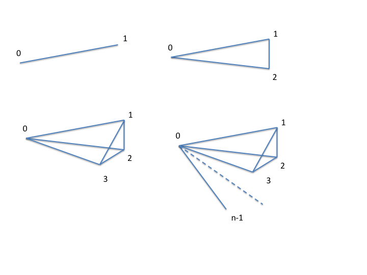
Figure 1: A cartoon illustrating two point correlation ($0-1$), three point correlation ($0-1-2$), four point correlation ($0-1-2-3$), and $n$ point correlation ($0-1-2-3-...-(n-1)$).

Let $\rho(X,Y,Z)$ be the density of the matter tracer (e.g. galaxy count per unit volume) at a location with Cartesian coordinates $(X,Y,Z)$, with the $\bar{\rho}(X,Y,Z)$ being the density of expected observations from tracers randomly distributed over with surveyed volume. We define the deviation from the average density as

$$\Delta(X,Y,Z)=\rho(X,Y,Z)-\bar{\rho}(X,Y,Z)\ .$$ (1)

The two point correlation can be visualized as an excess of sticks of a given length over the ones that are randomly distributed over space. The three point correlation corresponds to an excess of triangles, the four point correlation - to counting pyramids (the four points do not necessarily lie in one plane), etc (see Fig 1). We will refer to these figures as $n$-pletes.

Let us consider all possible $n$-pletes with one vertex at point $0$, characterized by a vector $\@vec{r}$, with sides radiating from this vertex equal to $s_{1},s_{2},...s_{(n-1)}$. In the isotropic case considered here the lengths of other sides and all angles are arbitrary.

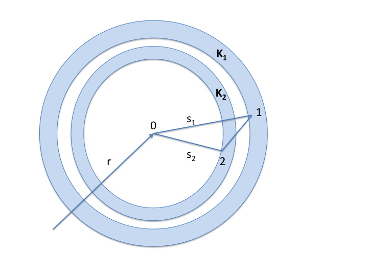
Figure 2: A cartoon illustrating three point correlation ($0-1-2$) with different scales $s_{1}$ on the side ($0-1$) and $s_{2}$ on the side ($0-2$). Integration over spherical shells $K_{1}$ and $K_{2}$ is equivalent to counting all possible triangles that have one vertex at point $0$ and the other two anywhere on the spheres.

The isotropic $n$-point correlation function ($n$pcf) is defined as

$$\xi_{n}(s_{1},s_{2},...s_{(n-1)})=\\ \frac{\int\Delta(\@vec{r})\Delta(\@vec{r}+\@vec{s_{1}})\Delta(\@vec{r}+\@vec{s_{2}})...\Delta(\@vec{r}+\@vec{s}_{(n-1)})d\@vec{r}d\Omega_{1}d\Omega_{2}...d\Omega_{(n-1)}}{\int\bar{\rho}(\@vec{r})\bar{\rho}(\@vec{r}+\@vec{s_{1}})\bar{\rho}(\@vec{r}+\@vec{s_{2}})...\bar{\rho}(\@vec{r}+\@vec{s}_{(n-1)})d\@vec{r}d\Omega_{1}d\Omega_{2}...d\Omega_{(n-1)}}\ .$$ (2)

where the integration over $\@vec{r}$ implies all possible positions of point $0$ in the surveyed volume. The integration over a solid angle $d\Omega_{i}$($i=1,...n-1$) between vectors $\@vec{s_{i}}$ and $\@vec{r}$ is equivalent to integration over a sphere of radius $s_{i}$ centered on point $0$, which, thus, evaluates the total number of tracers displaced from point $0$ by the distance $s_{i}$. This is illustrated in Fig. 2 for three point correlation. In term of Legendre polynomials expansion this definition of $n$pcf corresponds to $l=0$.

ConKer evaluates the integral of the $\Delta$ field on a spherical shell of radius $s_{i}$ by placing a spherical kernel $K_{i}$ on point $0$ with Cartesian coordinates $(X,Y,Z)$ and taking its inner product with the $\Delta$ field. Then the kernel is moved to a different location, thus scanning the entire surveyed volume. The results of each step, $W_{i}(X,Y,Z)$, is a map of weights that characterize the integral of the density deviation on a spherical shell of radius $s_{i}$ around the location $(X,Y,Z)$.

2.2 Input

The inputs to the algorithm are catalogs of the observed number count of tracers $D$, with the total number being $N_{tot}$, and $R$, which represents a number count of randomly distributed points within the same fiducial volume. Most surveys provide the angular coordinates: right ascension $\alpha$ and declination $\delta$, and the redshift $z$ of the tracer. The relationship between the redshift and the comoving radial distance is cosmology dependent:

$$r(z)=\frac{c}{H_{0}}{\displaystyle\int_{0}^{z}}\frac{dz^{\prime}}{\sqrt{\Omega_{M}(z^{\prime}+1)^{3}+\Omega_{k}(z^{\prime}+1)^{2}+\Omega_{\Lambda}}}\ ,$$ (3)

where $\Omega_{M}$, $\Omega_{k}$, and $\Omega_{\Lambda}$ are the relative present day matter, curvature, and cosmological constant densities respectively. $H_{0}$ is the present day Hubble’s constant, $c$ is the speed of light. These user-defined parameters represent the fiducial cosmology. The integral in Eq. 3 is evaluated numerically in ConKer. The comoving Cartesian coordinates are computed with:

$$X=r\cos(\delta)\cos(\alpha)\ ,$$ (4)

$$Y=r\cos(\delta)\sin(\alpha)\ ,$$ (5)

$$Z=r\sin(\delta)\ .$$ (6)

Cartesian coordinates are given as capital letters, $X$, $Y$, $Z$, as the redshift, $z$, is denoted in lower case.

We define a grid with spacing $g_{s}$, such that the volume of each cubic grid cell is $g_{s}^{3}$. $(X,Y,Z)$ denotes the Cartesian coordinates of the center of a grid cell. On this grid we define 3-dimensional histograms $D(X,Y,Z)$ and $R(X,Y,Z)$, which represent tracer counts in the cell $(X,Y,Z)$ from data and random catalogs respectively. These histograms may be populated by the raw count, or weighted count of tracers from the input catalogs. To properly account for the variation in angular completeness and the redshift selection function, the expected count from the random distribution, normalized to $N_{tot}$, is subtracted from the galaxy survey $D$ on the cell-by-cell basis. $R$ is evaluated using a random catalog. As an alternative, $R$ could be evaluated assuming that the tracers’ angular, $P_{ang}(\alpha,\delta)$ and redshift, $P_{z}(z)$ probability density distributions are factorizable (Demina et al., 2018). Then the expected count from the random distribution of galaxies in a Cartesian cell is:

$$R(X,Y,Z)=N_{tot}[P_{ang}(\alpha,\delta)\times P_{z}(z)]\frac{dXdYdZ}{dV_{sph}}\ ,$$ (7)

where $dXdYdZ$ and $dV_{sph}=r^{2}d\sin\delta d\alpha$ give the volume of a particular cell in Cartesian and spherical sky coordinates. This method of estimating the expected count from the random distribution reduces the statistical fluctuations compared to the count taken directly from the random catalog. Both methods are realized in the algorithm and may be chosen by the user.

A 3-dimensional local density variation histogram $N(X,Y,Z)$, which is a discretized representation of the $\Delta$ field, is then defined on the grid to represent the difference in counts between $D$ and $R$:

$$N(X,Y,Z)=D(X,Y,Z)-R(X,Y,Z)\ .$$ (8)

This stage of the algorithm is referred to as mapping.

2.3 Kernels

We construct $(n-1)$ spherical kernels, $K_{i}(X,Y,Z)$ on a cube of size $2s_{i}$ in all directions, just large enough to encompass a sphere of radius $s_{i}$. The grid defined on this cube has the same spacing, $g_{s}$, as the one used to construct $D(X,Y,Z)$. Grid cells intersected by a sphere of radius $s_{i}$ centered on the center of the cube, are assigned a value of 1. All other cells are 0.

2.4 Convolution

We construct a 3-dimensional histogram $W_{i}(X,Y,Z)$ with entries equal to the inner product of kernel $K_{i}$ centered on a cell with coordinates $(X,Y,Z)$ and matter density variation field $N$:

$$W_{i}(X,Y,Z)\equiv N(X,Y,Z)\ast\ast\ast K_{i}(X,Y,Z)\ ,$$ (9)

where $\ast\ast\ast$ denotes a 3-dimensional discrete convolution. One step in this process is visualized in Fig. 3.

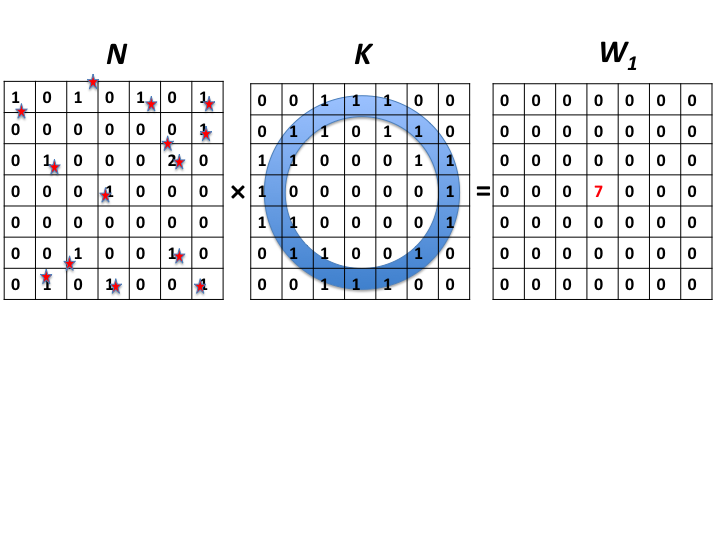
Figure 3: A 2-dimensional representation of one step in the convolution between the matter histogram $N$ (left) and the spherical kernel $K$ (center). In this example, the inner product is 7, which is placed in the center cell of $W_{1}$ histogram (right).

This procedure is realized using an $FFT$ in a highly vectorized algorithm. In this process, all $N(X,Y,Z)$ cells are interpreted once as center points, i.e. point 0 in Fig. 2, and other times as points on shells. Thus the 3-dimensional histogram $W_{0}(X,Y,Z)$ is approximated as simply being the density variation in each cell of $N(X,Y,Z)$, i.e. $W_{0}=N$.

For normalization purposes, we perform the same procedure on the field of random counts. The result of the convolution of random density field $R$ with kernel $K_{i}$ is referred to as $B_{i}(X,Y,Z)$:

$$B_{i}(X,Y,Z)\equiv R(X,Y,Z)\ast\ast\ast K_{i}(X,Y,Z)\ ,$$ (10)

This stage of the algorithm is referred to as convolution.

2.5 n-point correlation function

The $n$pcf, which approximates the one defined in Eq. 2 is calculated as:

$$\xi_{n}(s_{1},s_{2}...s_{(n-1)})=\frac{\sum W_{0}W_{1}W_{2}...W_{(n-1)}}{\sum B_{0}B_{1}B_{2}...B_{(n-1)}}\ .$$ (11)

The 2pcf is then

$$\xi_{2}(s_{1})=\frac{\sum W_{0}W_{1}}{\sum B_{0}B_{1}}\ .$$ (12)

The 3pcf necessitates convolution with kernel $K_{2}$ of radius $s_{2}$, resulting in weights $W_{2}$. The 3pcf is then calculated as

$$\xi_{3}(s_{1},s_{2})=\frac{\sum W_{0}W_{1}W_{2}}{\sum B_{0}B_{1}B_{2}}\ .$$ (13)

The stage of the evaluation of the $n$pcf is referred to as summation.

2.6 Equidistant case

Of particular interest are correlations between objects with a defined scale, such as those arising from a spherical sound wave in the primordial plasma, a.k.a. baryon acoustic oscillation. In this case, one tracer taken as a starting point is displaced from the rest $(n-1)$ points by the same distance $s_{1}$, e.g. the three point correlation corresponds to isosceles triangles randomly distributed in space. This equidistant case corresponds to the diagonal of the $n$-point correlation function, which is calculated as

$$\xi_{n}^{diag}(s_{1})=\frac{\sum W_{0}W_{1}^{n-1}}{\sum B_{0}B_{1}^{n-1}}\ .$$ (14)

Note that only $W_{0}$, $W_{1}$, $B_{0}$ and $B_{1}$ need to be evaluated, resulting in a substantial time saving.

2.7 Continuous matter distribution

The continuous matter distribution map that results from line intensity or weak lensing, differs from the discrete case because the map does not have the meaning of counts. It can instead be interpreted as a $\delta$-field, where $\delta$ has a meaning of relative over-density:

$$\delta(X,Y,Z)=\frac{D(X,Y,Z)-R(X,Y,Z)}{R(X,Y,Z)}\ ,$$ (15)

where $D$ and $R$ are continuous data and random fields defined on a grid, as is the $\delta$-field, which is identical to $W_{0}$ map. The convolution of $\delta$-field with kernels produces $W_{i}$ maps. Since $\delta$-field is already normalized by the random matter distribution it is not necessary to do it in the $n$-point correlation function, which is equal to:

$$\xi_{n}(s_{1},s_{2}...s_{(n-1)})=\sum W_{0}W_{1}(s_{1})...W_{(n-1)}(s_{(n-1)})\ .$$ (16)

The two point correlation function is then

$$\xi_{2}(s_{1})=\sum W_{0}W_{1}\ .$$ (17)

2.8 Cross-correlation between different tracers

The algorithm can be used to evaluate cross-correlation between different tracers. In this case we have two (possibly background subtracted) matter maps $\Delta_{0}$ and $\Delta_{1}$. Then map of weights $W_{0}$ is equal to $\Delta_{0}$, and $K_{1}$ is convolved with $\Delta_{1}$ resulting in $W_{1}$. The two point correlation function is then evaluated according to Eq. 17 or Eq. 12 depending on whether the tracer counts are normalized to the random distribution or not.

3 Performance study

We evaluate the performance of ConKer using SDSS DR12 CMASS galaxies (Ross et al., 2017), their associated random catalogs, and an ensemble of MultiDark-Patchy mocks (Kitaura et al., 2016; Rodríguez-Torres et al., 2016). We apply ConKer to the SGC and NGC catalogs for data, randoms, and 40 mocks. In this performance study, we used the following values for the cosmological parameters: $c=300000$ km$/$s, $H_{0}=100h$ km$/$s$/$Mpc, $\Omega_{M}=0.307$, $\Omega_{\Lambda}=0.693$, and $\Omega_{k}=0$. This choice was motivated by the cosmological parameters used in the generation of the mock catalogs. For this study, which highlights the algorithm’s ability to probe correlations near the BAO scale, we compute correlation functions for a distance range of $54.8\mbox{---}139.8$ $h^{-1}$Mpc in 17 bins of width of $5$ $h^{-1}$Mpc. In all cases, the standard systematic (Ross et al., 2017) as well as FKP weights (Feldman et al., 1993) were used to create the density field map. The grid spacing for each run (with the exception of the timing study discussed in § 3.2) is $g_{s}=5$ $h^{-1}$Mpc.

3.1 Distance calibration

As in any algorithm that uses a map of tracers defined on a grid, there is a certain degree of degradation in the precision of the distance between the tracers. It is important to quantify the precision of distance determination. We calibrate the distance using a subsample of a random catalog, where we compare the distance measured on the grid with the one determined by a brute force calculation. Figure 4 shows the dependence of the mean true distance on the kernel size. The shaded region correspond to the RMS of the distribution in the true distance given a particular value of the kernel size, which is shown in the inset for a kernel size of 60 $h^{-1}$Mpc. The RMS is approximately 2.5 $h^{-1}$Mpc, which corresponds to one half grid spacing. The calibration procedure must be performed using a random catalog for each value of the grid spacing, $g_{s}$.

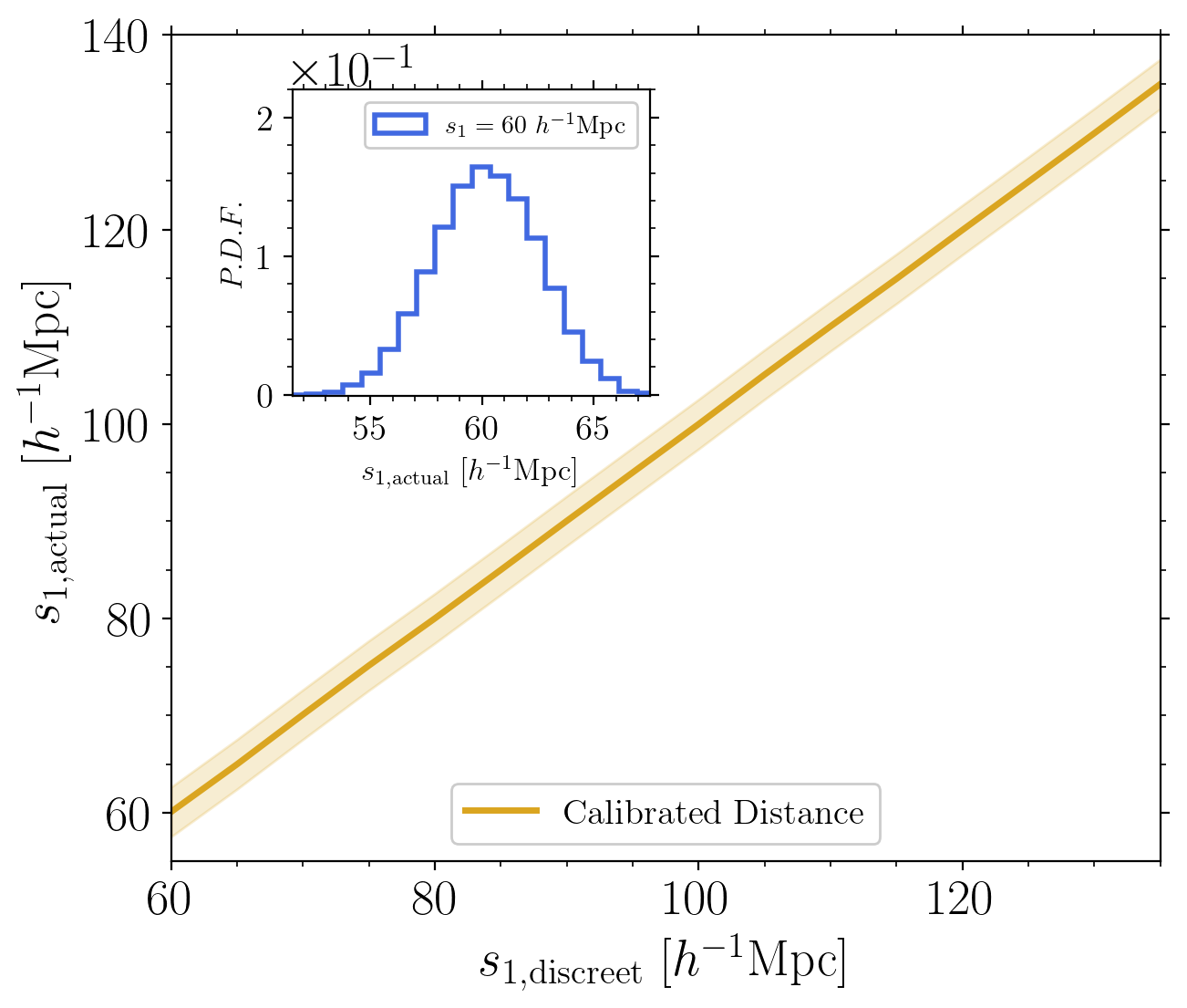
Figure 4: The true distances between the tracers and the center of the kernel vs the discretized estimation of the distance in ConKer (gold). The shaded region gives the RMS of the true distance distribution. The inset shows one such distribution for a kernel with size $s_{1}=60$ $h^{-1}$Mpc.

3.2 Timing study

We present the analytical considerations of the time complexity of the three stages of the algorithm: mapping, convolution and summation in Appendix A.1. Here we show the results of the timing study performed using a personal computer with a 2.3 GHz Intel Core i7 processor and 8 GB of memory. All execution times are in units of CPU seconds.

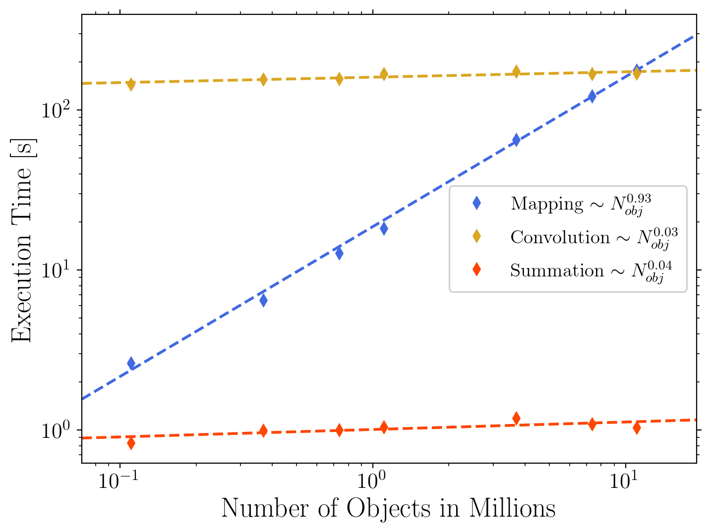
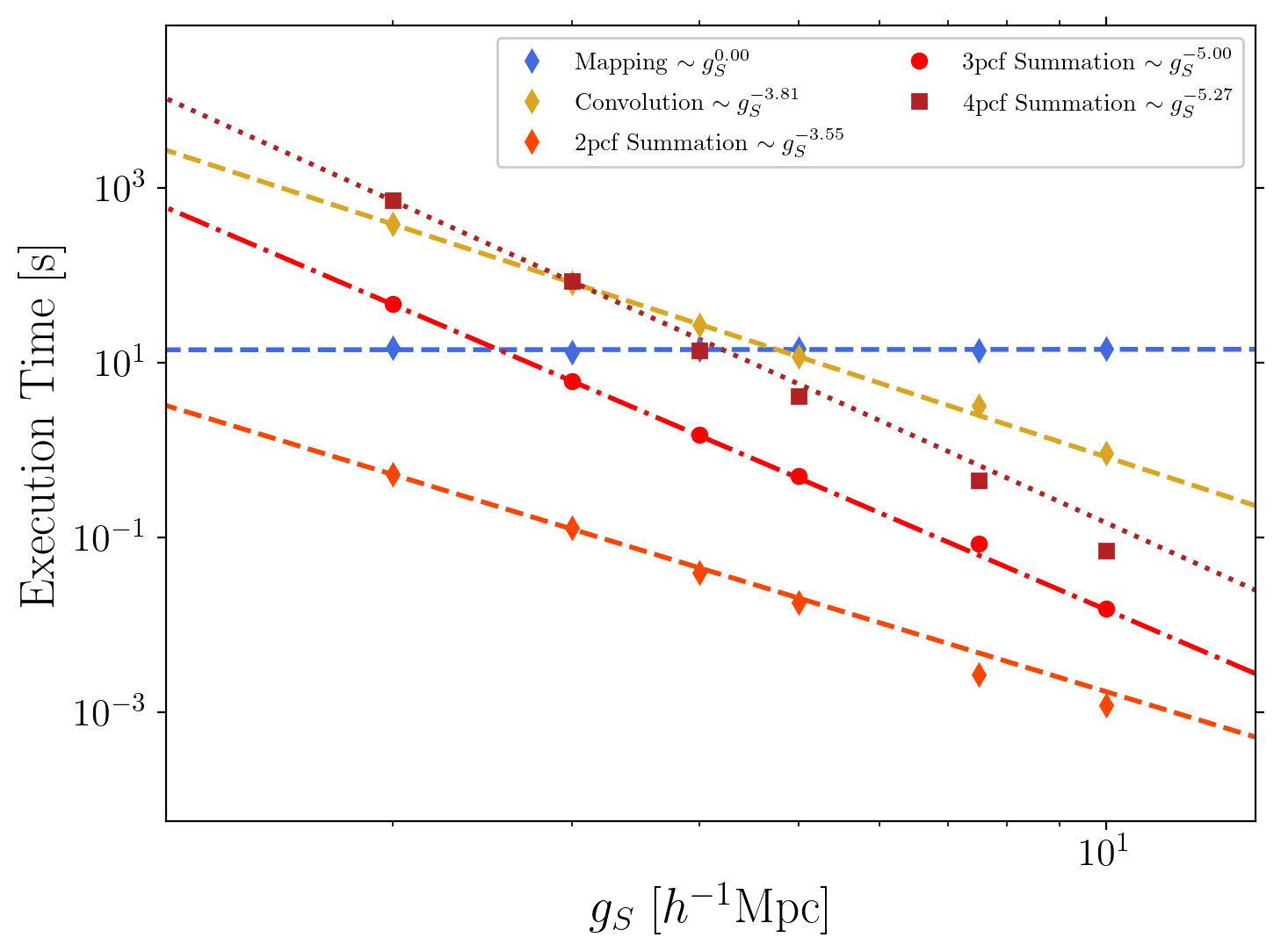
Figure 5: Color inline. The execution time of ConKer as applied to subsamples of the SDSS DR12 CMASS SGC galaxies. Top: the dependence on the number of combined data and random objects, using a grid spacing $g_{S}=5$ $h^{-1}$Mpc. Bottom: the dependence on the grid spacing, $g_{S}$, for 0.87M objects. Points present the measured time. Lines are the results of the fit to a power law, with the scaling given in the legend.

The primary advantage of ConKer is in the behavior of the execution time as a function of the number of objects, $N$, shown in top plot of Fig. 5 for the three stages of the algorithm. The surveyed volume, $V$ is kept fixed. As expected the execution time of both convolution and summation are independent of $N$. Mapping is a $\mathcal{O}(N)$ calculation, and starts dominating for catalogs larger than 10M objects.

The main parameter that determines the computation time of ConKer is the number of grid cells, $N_{c}$, which depends the grid spacing, $g_{s}$ (see the bottom plot of Fig 5 for $n=2,3,4$). Mapping is independent of $g_{s}$. For 2pcf convolution is expected to scale as $g_{s}^{-4}\log g_{s}$, and summation as $g_{s}^{-4}$. Both parts scale somewhat slower than expected. The execution time of convolution is independent of the correlations order $n$. Each additional order of correlation is expected to add one power of $g_{s}$ to summation time. This is roughly in agreement with the observed dependence for 3pcf and 4pcf. Summation starts dominating the execution time for 4pcf for grid spacing below 2 $h^{-1}$Mpc. For $n>4$ the execution time is expected to be dominated by summation, which is a $O(N_{c}^{(n+2)/3})$ calculation. For lower $n$ or higher grid spacing convolution is the dominant part, expected to be $O(g_{s}^{-4}\log g_{s})$, or $O(N_{c}^{4/3}\log N_{c})$.

The algorithm’s memory requirements are discussed in Appendix A.2.

3.3 Comparison to nbodykit

We present a comparison of the 2pcf and 3pcf evaluated using ConKer and nbodykit (Hand, 2018). The latter uses more traditional pair-counting methods, and may be used to evaluate the performance of ConKer. In nbodykit, the 2pcf is defined according to the estimator of Landy and Szalay (Landy & Szalay, 1993; Hamilton, 1993):

$$\hat{\xi_{2}}(s)=\frac{DD(s)-2DR(s)+RR(s)}{RR(s)}\ ,$$ (18)

where $DD$, $RR$, and $DR$ are the normalized distributions of the pairwise combinations of galaxies from data, $D,$ and random, $R,$ catalogs (plus cross terms) at given distances $s$ from one another. The nbodykit 3pcf is defined according to Slepian & Eisenstein (2015) and we consider the $\ell=0$ (isotropic) case. This corresponds to the ConKer 3pcf.

Using nbodykit, the 2pcf and 3pcf are calculated for the SGC sample of the SDSS DR12 CMASS galaxies and randoms. Due to the restriction that the 3pcf algorithm in nbodykit scales as $\mathcal{O}(N^{2})$ (Slepian & Eisenstein, 2015), where $N$ is the number of objects, the random catalog was reduced to 1M objects. Full random catalogs were used when running ConKer. The data catalog remained unchanged in both cases. The ConKer 3pcf was completed in $350s$ and the nbodykit 3pcf in $9870s$.

The comparison between the two methods of computing the 2pcf is given in Fig. 6. The two algorithms agree with one another across the entire range of $s_{1}$, and the residual between the 2pcf using ConKer and nbodykit is around an order of magnitude lower than the the value of $\xi_{2}$. The observed small differences are due to the precision of the distance determination on the grid in ConKer resulting in some bin-to-bin migrations, while nbodykit calculates the actual distance between the two points.

We repeat this procedure with the on and off diagonal elements of the 3pcf (Fig. 7). Here, both methods agree as well, as demonstrated by the residual between the two methods shown in the bottom right of Fig. 7. Some difference is due to the reduction in the size of the randoms catalog for the nbodykit calculation, which leads to larger statistical fluctuations. Overall, ConKer is in a good agreement with standard algorithms, and has the unique advantage of being able to probe higher order correlations as well, with relatively little increase in run-time.

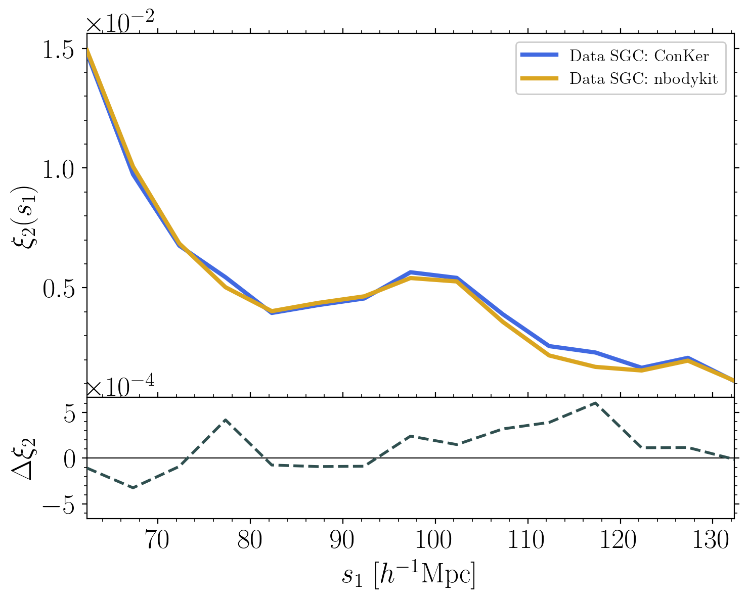
Figure 6: The top panel shows the 2pcf, $\xi_{2}(s_{1})$, for the CMASS galaxy sample of the SDSS DR12 survey computed using ConKer (blue) and the 2pcf computed using nbodykit (gold). The bottom panel gives the residual between the two, defined as $\xi_{2,{\tt ConKer}}-\xi_{2,{\tt nbodykit}}$ (grey dashed line). The solid black line in the bottom panel shows $\Delta\xi_{2}=0$.

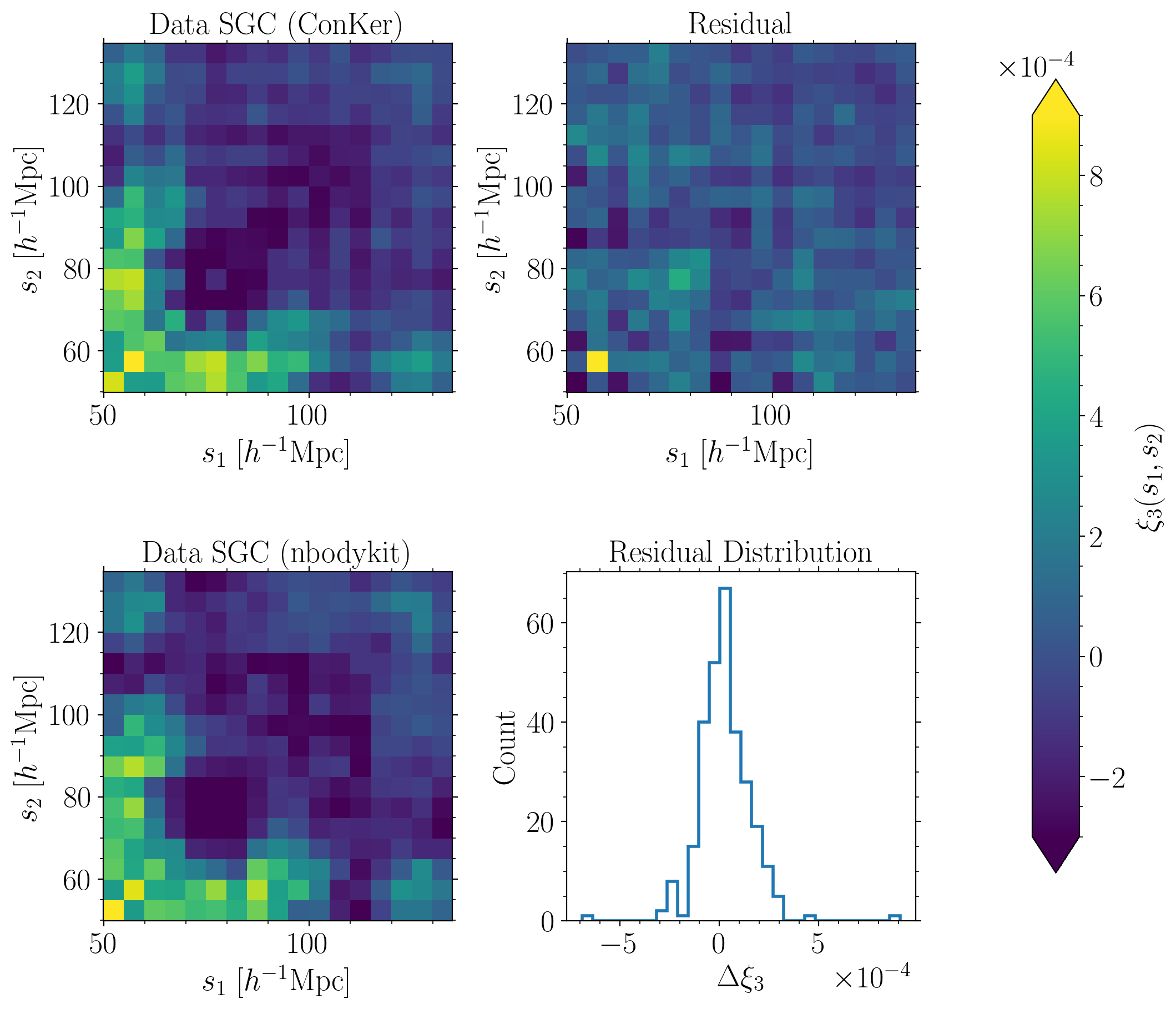
Figure 7: The top left panel shows the 3pcf, $\xi_{3}(s_{1},s_{2})$, for the CMASS galaxy sample of the SDSS DR12 survey computed using ConKer and the bottom left panel shows the 3pcf computed using nbodykit. The top right panel gives the residual between the two, defined similarly as $\xi_{3,{\tt ConKer}}-\xi_{3,{\tt nbodykit}}$. The color scale corresponds to all three color panels. The bottom right panel gives a distribution over the residuals. The RMS of this distribution is $1.34\times 10^{-4}$.

3.4 ConKer npcf

We use ConKer to compute the diagonal elements of the $n$pcf for $n=2,3,4,5$ and off diagonal elements of the 3pcf for the SGC and NGC catalogs. The combination of NGC and SGC catalogs is done by adding together terms in the numerator and denominator of Eq. 11. For example, the combined 3pcf is given by

$$\xi_{3}(s_{1},s_{2})=\frac{\sum(W_{0}W_{1}W_{2})_{\mathrm{SGC}}+(W_{0}W_{1}W_{2})_{\mathrm{NGC}}}{\sum(B_{0}B_{1}B_{2})_{\mathrm{SGC}}+(B_{0}B_{1}B_{2})_{\mathrm{NGC}}}\ .$$ (19)

The diagonal elements of the $n$pcf’s $n=2,3,4$ and $5$ are shown in Fig. 8. We observe the expected features of the $n$pcf’s based on both mock and data catalogs. These include an increase in magnitude at small scales, corresponding to galaxy clustering, and a well defined ‘bump’ at the BAO scale. The $n$pcf’s based on the random catalog fluctuate about $\xi_{n}=0$ at several orders of magnitude below the signal observed in mocks and data.

Both on and off diagonal elements of the 3pcf are shown in Fig. 9. The diagonal elements in Fig. 9 directly correspond to the values in the second panel of Fig. 8. Off the main diagonal, we observe an increase in the magnitude of $\xi_{3}$ around $s_{1}=100$ and $s_{2}=60$ $h^{-1}$Mpc for data and mocks. The randoms show no clustering or BAO signal and fluctuate about $\xi_{3}=0$.

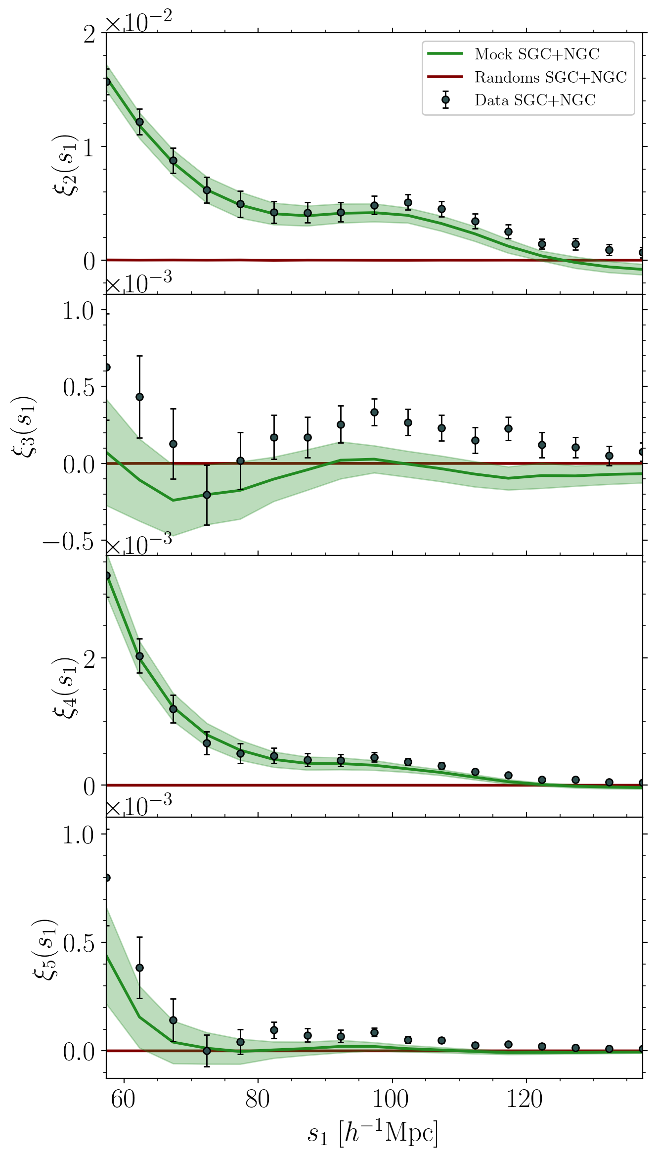
Figure 8: The diagonal $n$pcf, $\xi_{n}(s_{1})$, from $n=2$ to $n=5$ (top to bottom panels), for the combined SGC+NGC CMASS galaxy sample of the SDSS DR12 survey (black), the average of the ensemble of MD Patchy mocks (green) and the associated randoms (red). The green shaded region gives the standard deviation across mock catalogs, which is also used to generate the error bars associated with the data catalogs.

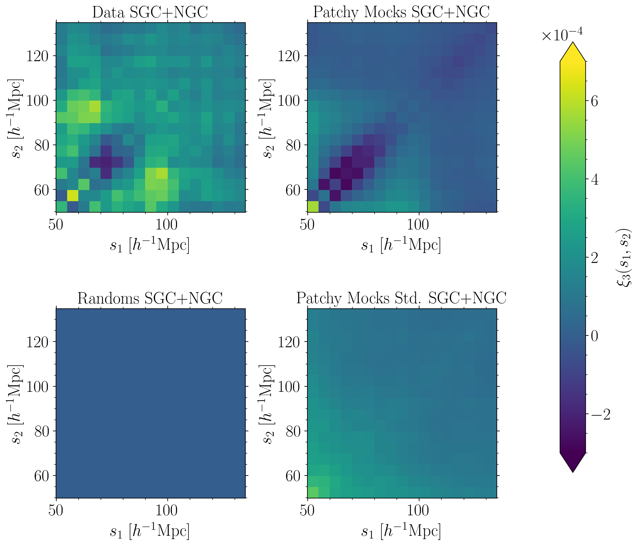
Figure 9: The 3pcf calculated based on data (top left), random (bottom left), and mock (top right) catalogs, using the combined SGC and NGC samples. The panel in the bottom right shows the standard deviation across the mock ensemble. The color scale corresponds to all four panels.

4 Discussion

4.1 Algorithmic framework

The query for a pattern in matter distributions may prompt an employment of machine learning techniques. ConKer, being a spatial statistics algorithm offers an alternative to such approach that is fast and transparent. It exploits the fact that the full set of equidistant points from any given point makes a sphere, with its surface density being a direct measure of how spherically structured this subspace of points is. Aggregating and combining this measure over the whole space of $N$ objects allows us to calculate the space’s $n$ point correlation function.

The algorithm exploits an intrinsic spatial proximity characteristic in the objective of querying for structures of negligible dimensions in a much bigger space. This spatial proximity factor leads to space partitioning algorithms targeting a nearest neighbor query approach, see for example the tree-based $n$pcf algorithms in March (2013). However, ConKer uses this fact as a heuristic in limiting its query space immediately to only the defined separation for each point in the space. Note how this is in contrast with the former technique family. In a nearest neighbor approach to the $n$pcf problem, the query space is grown at each point in the greater embedding space, aggregating the $n$-point statistic until the greater space is fully queried, whereas ConKer aggregates the statistic over all embedding space, and then grows the query space before repeating.

This design choice realized in ConKer’s core subroutine, a convolution of the query space with the embedding space performed by an $FFT$ algorithm, distills the complexity from the brute force $\mathcal{O}(N_{c}^{2})$ to $\mathcal{O}(N_{c}logN_{c})$, where $N_{c}$ is the total number of grid cells in a discrete 3-dimensional map. This approach, combined with the heuristic above, lets the dominant components of ConKer achieve independence of the number of objects as shown in Fig. 5. There is certainly a trade-off between the sparsity of the whole space and the bias towards linear complexity in number of objects, as expected from an $FFT$-based algorithm, but even for very dense catalogs, we expect the scaling in the number of objects to be capped by $\mathcal{O}(N)$, where $N$ is the total number of objects. Ultimately, ConKer is a hybrid algorithm that draws from both computational geometry and signal processing to achieve linear complexity in the number of objects.

4.2 Applications beyond correlation functions

Though traditionally the order of correlation $n$ is viewed as an important parameter, for the equidistant $n$pcf, all the information is entirely encoded by the weights $W_{0}$ and $W_{1}$. It was pointed out in Carron & Neyrinck (2012) that the $n$pcf is inadequate in capturing the tails of non-Gaussianities. The distributions over $W_{0}$ and $W_{1}$ (as opposed to their sum over the sample as is used in the $n$pcf) could recover that sensitivity, which is a subject for future studies. The distribution of the product of two weights, $W_{0}W_{1}$ normalized by the average $B_{0}B_{1}$ is presented in Fig. 10 for the kernel size of 107.3 $h^{-1}$Mpc for data, mock and random catalogs.

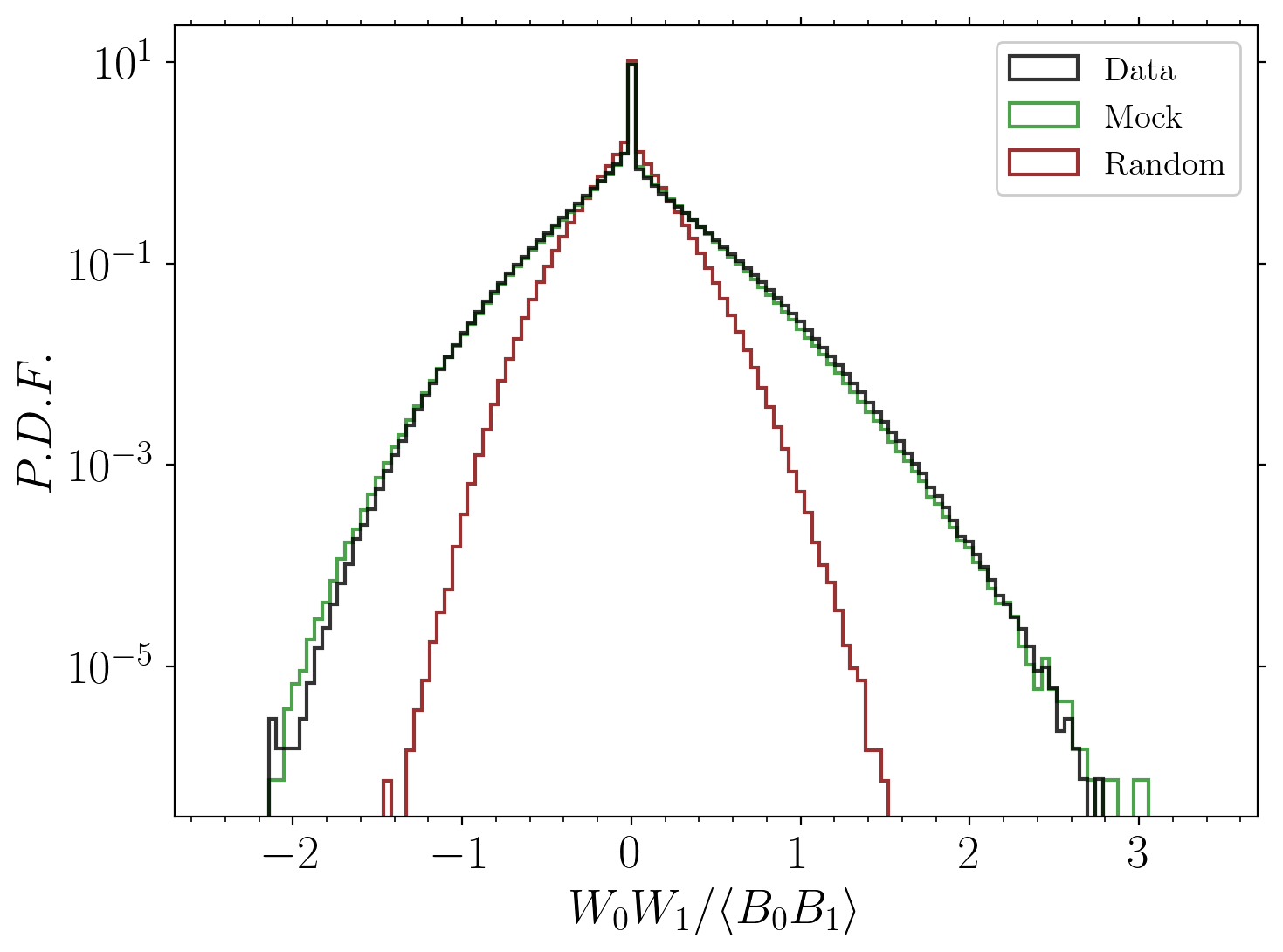
Figure 10: The distribution, $W_{0}W_{1}/\langle B_{0}B_{1}\rangle$ at $s_{1}=107.3$ $h^{-1}$Mpc, for the CMASS galaxy sample of the SDSS DR12 survey (black), one of the MD Patchy mocks (green) and the associated randoms (red). This plot includes SGC galaxies only.

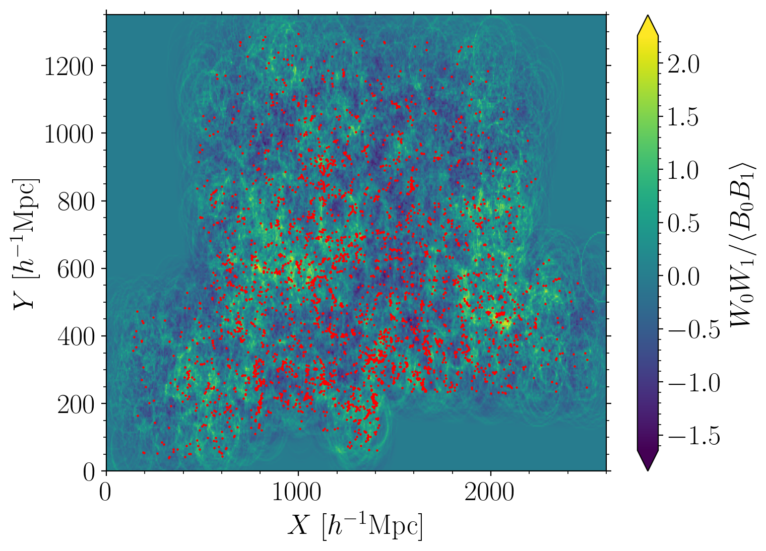
Figure 11: A 5 $h^{-1}$Mpc thick slice of the SDSS DR12 SGC volume, where the color scale shows the value of $W_{0}W_{1}/\langle B_{0}B_{1}\rangle$ at $s_{1}=107.3$ $h^{-1}$Mpc, and the red stars indicate the positions of galaxies.

Moreover, $W_{0}$ and $W_{1}$ as well as their product are maps. While in the $n$pcf, the location information is entirely lost, in the maps produced by ConKer, it is preserved and can be used for cross correlation studies between different tracers, such as weak lensing, Ly$\alpha$ and CMB. The preservation of this spatial information is illustrated by Fig. 11, where the DR12 SGC galaxies are plotted on top of the values of $W_{0}W_{1}/\langle B_{0}B_{1}\rangle$ for a kernel size approximately equal to the BAO scale. The figure corresponds to a slice of thickness 5 $h^{-1}$Mpc. The observed circles around the boundaries of the catalog or the sparsely populated regions are a feature of the algorithm, since a single galaxy contributes to $W_{1}$ everywhere at a distance $s$ from the galaxy forming a sphere. The highest values in the map (yellow color scale) correspond to the regions that are both densely populated and have several galaxies displaced by a given scale from this point, as one would expect from the centers of the baryon acoustic oscillations. Similarly, lowest values (blue color scale) correspond to under-dense regions and troughs of BAO originating from this location. Such an aggregated approach gives access to the matter distribution in the early universe.

5 Conclusion

We presented ConKer, an algorithm that convolves spherical kernels with matter maps allowing for fast evaluation of the isotropic $n$-point correlation functions. The algorithm can be broken into three stages: mapping, convolution and summation. Execution time of convolution and summation are independent of the catalog size, $N$, while mapping is a $\mathcal{O}(N)$ calculation, which starts dominating for catalogs larger than 10M objects. For the correlation orders $n<5$, convolution is the dominant part with complexity $\mathcal{O}(N_{c}^{4/3}\log N_{c})$, where $N_{c}$ is the number of the grid cells. For higher $n$ the overall time complexity is dominated by summation, which is $\mathcal{O}(N_{c}^{(n+2)/3})$.

Comparison to the standard techniques shows a good agreement. We study the performance using SDSS DR12 CMASS galaxies, their associated random catalogs, and an ensemble of MultiDark-Patchy mocks. The results up to $n=5$ are presented. Further metrics that may offer additional sensitivity to primordial non-Gaussianities are also suggested (e.g. distribution over weights $W_{i}$).

Appendix A Algorithm requirements

A.1 Estimation of time complexity

Let us define the relevant parameters:

• $N$ - number of objects in catalog (since random catalogs are larger, their size is the leading contribution);

• $n$ - order of the correlation;

• $g_{s}$ - grid spacing;

• $V$ - volume of a Cartesian box that fully encloses the surveyed region;

• $N_{c}=V/g_{s}^{3}$ - number of grid cells;

• $s$ - separation of galaxies probed;

• $s_{max}$ - maximum separation of galaxies probed;

• $N_{s}=s_{max}/g_{s}=s_{max}(N_{c}/V)^{1/3}$ - number of steps in $s$;

• $V_{k}=s^{3}$ - kernel volume for galaxy separation $s$;

• $N_{k}=V_{k}/g_{s}^{3}$ - number of grid cells in kernel volume.

Here we present the evaluation of the time complexity of the three stages of the algorithm: mapping, convolution and summation.

1. Mapping - $O(N)$

   Since $N$ objects must be placed in grid cells, the time complexity of the mapping is proportional to $N$:

   $$t_{1}\propto N\,.$$ (20)

   It does not depend on neither $n$, $N_{c}$, nor $N_{k}$.

2. Convolution - $O(N_{c}^{4/3}\log N_{c})$

   Convolution of cubic volumes of the size $N_{k}$ is performed using $FFT$ $N_{c}$ times at each step in $s$. Hence the complexity of each step is $O(N_{c}\log N_{k})$. The kernel size itself depends on $s$. We can put an upper bound on it at $s_{max}$. The time complexity of the convolution is:

   $$t_{2}\propto N_{s}N_{c}\log N_{k}<\frac{s_{max}}{g_{s}}\frac{V}{g_{s}^{3}}\log\frac{V_{k}}{g_{s}^{3}}\propto g_{s}^{-4}\log g_{s}\propto N_{c}^{4/3}\log N_{c}\,.$$ (21)

   We note that the time complexity of convolution does not depend neither on $n$, nor on $N$, and is the same for on and off diagonal elements.

3. Summation: full -$O(N_{c}^{(n+2)/3})$, diagonal - $O(N_{c}^{4/3})$

   At each one of the $N_{s}$ steps a product of $n$ grids, each of dimensionality $n$ with each side having a length of $\sqrt[3]{N_{c}}$ is evaluated, assuming cubic grids. Most of these products are identical. The number of unique combinations calculated is $\pmatrix{N}_{s}\\ n-1$, which contains $(n-1)$ terms. Hence the time complexity of summation is

   (22)

   (23)

   nNc∝n(smaxgs)(n-1)Vgs3∝gs-(n+2)∝Nc(n+2)/3.

   For a special case of evaluating only the diagonal elements of $n$pcf the algorithm takes a product of $n$ arrays each $N_{c}$ long $N_{s}$ times, hence the time complexity of summation is

   $$t_{3}^{diag}\propto nN_{c}N_{s}\propto n\frac{s_{max}}{g_{s}}\frac{V}{g_{s}^{3}}\propto g_{s}^{-4}\propto N_{c}^{4/3}\,.$$ (24)

   We note that for a general case for $n>2$ summation has the highest complexity and becomes dominant for very low values of grid spacing. For the diagonal elements the complexity of this stage is $N_{c}^{4/3}$, or lower than that of the convolution stage.

   A.2 Estimation of memory requirements

   A run of ConKer necessitates several discrete maps that span the survey volume to be held on RAM. For instance, calculating the 2pcf of SDSS DR12 CMASS SGC galaxies with a grid spacing of $5$ $h^{-1}$Mpc produces maps of approximate dimensions ($400^{3}$). Assuming a 64-bit underlying architecture and grids populated by single-precision floating point numbers, such a contiguous block of memory is just under a Gigabyte. A full run on SGC galaxies needs an available run time memory in the lower single digits in Gigabytes. This memory requirement increases for larger catalogs, but only in proportion to the additional survey volume.

   ConKer also requires more memory when computing the off-diagonal elements of higher order $n$-point correlations as opposed to computing just diagonal elements. This is due to the fact that for off-diagonal correlations, the algorithm needs to store the grids corresponding to the convolution of the density grid with each kernel size in the scan, $K_{i}$, until the very end of the scan, whereas for a diagonal correlation it simply discards the grids at each consecutive scale. Since this algorithm is purposed for use on calculating the $n$pcf at discrete separation values with the total number of such steps being in the low double digits, memory scaling for the off-diagonal case remains feasible on any modern personal computer.