Long-Range Optical Wireless Information and Power Transfer

Abstract

Simultaneous wireless information and power transfer (SWIPT) is a remarkable technology to support both the data and the energy transfer in the era of Internet of Things (IoT). In this paper, we proposed a long-range optical wireless information and power transfer system utilizing retro-reflectors, a gain medium, a telescope internal modulator to form the resonant beam, achieving high-power and high-rate SWIPT. We adopt the transfer matrix, which can depict the beam modulated, resonator stability, transmission loss, and beam distribution. Then, we provide a model for energy harvesting and data receiving, which can evaluate the SWIPT performance. Numerical results illustrate that the proposed system can simultaneously supply 0$\sim$9 W electrical power and 18 bit/s/Hz spectral efficiency over 20 m distance.

I Introduction

In the era of Internet of Things (IoT), countless network devices are interconnected in various scenarios for making our life smart and convenient. However, with expansion of applications of IoT, their demands for communication and power increase dramatically [1, 2, 3, 4, 5]. Facing this bottleneck, simultaneous wireless information and power transfer (SWIPT) technology has recently attracted wide attention to providing both information and energy at the same time [6]. SWIPT technologies can be classified into two types: wide-area omnidirection and narrow-beam orientation. Wide-area omnidirectional technology such as broadcasting radio-wave can support long-distance and omnidirectional SWIPT [7]. But, the broadcasting energy emission results in energy dissipation, which makes it difficult to achieve high-power transmission. Narrow-beam orientation technology such as beamforming light-emitting diode/laser diode can support high energy density transmission [8]. But using the narrow electromagnetic beam always accompanies the challenges of alignment and human safety. The emergence of scheme based on resonant beam (RB) provides a new idea to implement SWIPT.

The RB scheme utilizes the optical beam as the energy and data carrier, which belongs to the narrow-beam type. Moreover, due to the line of sight (LoS) characteristic, the beam delivering will cease immediately when objects intrusion, which can ensure safety. Besides, thanks to the separation cavity structure and retro-reflectors, the system can realize self-alignment for mobility [9]. Furthermore, the optical beam enables the ability of high-rate data transfer because of the huge available bandwidth and high signal-to-noise ratio[10]. Fig. 1 depicts the application scenarios of the RB system. Devices such as the unmanned aerial vehicle (UAV), smartphones, laptops, etc., can be supported by it [11].

The original RB (also known as distributed laser) design was proposed by [12] for wireless power transfer. It immediately gains wide attention. In [13], Zhang et al. concluded the function principle, built the numerical model, and analyzed the basic performance of the RB system for wireless charging. Zhang et al. also experimentally confirm that the energy transfer of the RB system can accomplish 2 W power transfer over 2.6 m [14]. In [15], Sheng et al. shows an efficient, long-distributed-cavity laser that uses a cat-eye retroreflector arrangement to enable cavity alignment, a telescope to broaden and focus the laser beam, as well as analyzing the impact of intra-cavity spherical aberration on laser efficiency and correcting it with an aspheric lens. Sheng et al. also studied the theoretical and practical effects of field curvature (FC) on a distributed-cavity laser with cat-eye optics [16]. The RB system use light beam as carrier, which makes it have great communication potential. In [17], Xiong et al. shows a feasible wireless communication scheme based on RB, as known as, resonant beam communications (RBCom). Xiong et al. also proposed a second-Harmonic RBCom design which is used to overcome the echo-interference problem during the data transfer [18].

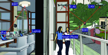
Figure 1: Resonant beam systems application scenarios (RBT: resonant beam transmitter; UAV: unmanned aerial vehicle)

In summary, the above research has explored the RB technology on system design, basic principle development, and structure optimization in power charging and communication, which builds a preliminary notion for RB-SWIPT. However, the resonant beam SWIPT technology still has challenge in feasible system design, performance evaluation, and parameters analysis. In this paper, we introduce a long-range simultaneous wireless information and power transfer scheme based on RB. Then, we adopt the transmission matrix to analyze the end-to-end beam transfer, resonator stability, and beam distribution. We also present an analytical model for simultaneous power and data transfer. Finally, we evaluate the system performance and give analysis for structure parameters.

The contributions of this paper can be concluded as follows:

• An optical wireless information and power transfer (LOWIPT) system is proposed, which can concurrently achieve long-range, high-power charging, and high-rate communication for IoT devices.

• The end-to-end beam transmission process is revealed utilizing the beam transmission matrix, which can analyze the beam modulated, resonator stability, transmission loss, and beam distribution.

• The model of simultaneous power and data transfer is developed, based on which the LOWIPT performance can be evaluated and analyzed.

The presentation of the system fundamental concept will be illustrated in Section ii@ of the rest of this paper. The BCRB system’s analytical model will be developed in Section iii@. The performance of the BCRB system will be evaluated in Section iv@. Finally, in Section v@, conclusions will be drawn.

II System Fundamental Principle

Fig. 2 depicts the design of the RB-SWIPT system. The system is divided into two parts: the transmitter and the receiver, which are separated by free space. A reflector M1, a power source, a gain medium, and a TIM are in the transmitter. A reflector M2, a beam splitter, a photovoltaic (PV) cell, and an avalanche photodiode (APD) are in the receiver. Among these elements, the reflectors M1, M2, TIM, and the gain medium form the spatially separated resonator (SSR), based on which the resonant beam can be transmitted. In the following subsections, we will briefly outline the fundamental principles of energy conversion and data transfer, as well as influence factors about the long-range resonant beam transfer.

II-A Energy Conversion

The system’s energy conversion process is separated into three phases: energy absorption, stimulated emission, and power output. 1) Energy absorption: The input electrical power is converted to pump beam power in the power source. Then, with the pump beam radiating to the gain medium, the particles in the gain medium will be activated, which leads the particles being transited from low energy level to high energy level. Finally, population inversion occurs and energy is stored in the gain medium. 2) Stimulated radiation:Particles are continually transited to the high energy level with the pump power input. Because high-energy particles are in the unstable state, they will fall back to a lower energy level with spontaneous and stimulated radiation and produce photons. 3) Power output: These released photons forming the beam rays travel between the reflectors M1 and M2, accompanied by energy gain and loss. During this process, part of the beam that carry the energy will output at M2 of the receiver.

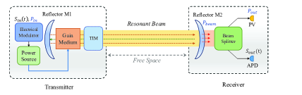
Figure 2: System diagram (TIM: telescope internal modulator; PV: photovoltaic; APD: avalanche photodiode; $S_{\mathrm{in}}$, $S_{\mathrm{out}}$: input and output signal; $P_{\mathrm{out}},~{}P_{\mathrm{in}}$: output, input electrical power)

II-B Data Transfer

The data signal is loaded on the pump source by an electrical modulator, as shown in Fig. 2. The gain medium receives the pump energy and generates the excitation beam where the mapping relationship can be built and the signal can be delivered into the SSR. Then, after the beam transmitting through the free space from transmitter to receiver, the signal will be received by the APD detector. The communication process of the proposed system is similar to traditional space optical communication, which can be modeled as a linear time-invariant system [19]:

$${\color[rgb]{0,0,1}S_{\mathrm{out}}(t)=\gamma P_{d}S_{\mathrm{in}}(t)\ast(h_{s}(t)\ast h_{f}(t)\ast h_{D}(t))+n_{t}(t),}$$ (1)

where $\ast$ is the convolution operator, $S_{\mathrm{out}}$ and $S_{\mathrm{in}}$ express the output signal and input signal; $n(t)$ is the additive white Gaussian noise (AWGN), and $h_{s}(t)$, $h_{f}(t)$, $h_{D}(t)$ are the impulse response functions of the adjustable power source, the free space and the APD detector, respectively.

II-C Transmission Loss

Section II.A states that there are several phases involved in the conversion of energy, accompanying by energy loss such as heat loss, air absorption loss, optical reflection loss, and beam diffraction loss. Among them, beam diffraction loss belong to transmission loss which will gain as the distance increase, impacting the transfer range. The beam diffraction loss comes from the beam diffraction and overflow on the finite aperture [20]. In Fig. 3, we assume that a beam with a divergence angle $\theta$ and beam spot (beam cross-section) radius $\omega$ spreads in open space. Due to $\theta$, the beam will inevitably diffusion during transmission, which makes the spot radius enlarge from $\omega$ to $\omega^{\prime}$. When there is an aperture with radius $a$ ($a<\omega^{\prime}$) in the transmission route, a portion of the beam will overflow or become obstructed, resulting in beam loss. Moreover, since the beam divergence increases with distance, the loss will gain, continuously. Finally, the beam transmission is cut off when the energy loss is big enough over a given distance. Generally, if the beam spot is substantially bigger than the aperture, significant energy loss will present. In contrast, energy loss will be minimal if the beam spot is manageable and the majority of the beam may travel through the aperture instead of being obstructed or overflowing [21, 22].

In the RB system, elements such as gain medium and reflectors with geometric boundary will be as apertures in the transmission route. On this premise, TIM was proposed and introduced into the proposed scheme to suppress the transmission loss, which will be described in the next chapter.

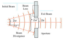
Figure 3: Beam loss on aperture ($\omega$: initial beam radius; $\omega^{\prime}$: divergent beam radius; $a$: aperture radius; $\theta$: divergence angle)

III Analytical Model

In this section, we will depict the end-to-end beam transmission using the transmission matrix at first. Then, we will define the beam distribution. Finally, the model of energy output and data transfer will be developed. These models lay an analytical foundation for the performance evaluation of the RB-SWIPT system in Section IV.

III-A End-to-end Beam Transmission

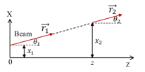
Figure 4: Beam propagating in the free space expressing by vector ($\vec{r_{1}}$:beam with location $x_{1}$ and $\theta_{1}$ angle; $\vec{r_{2}}$:beam with location $x_{2}$ and $\theta_{2}$ angle; $z$: $\vec{r_{2}}$ location on the Z axis)

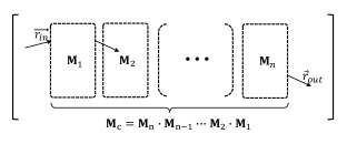
Figure 5: Beam propagation in concatenate elements ($\vec{r_{\mathrm{in}}}$: Initial beam vector; $\vec{r_{\mathrm{out}}}$: Exit beam vector; $\mathbf{M}_{1}$-$\mathbf{M}_{n}$: transmission matrices)

1) Transmission matrix: To establish the analytical model of the beam transmission, the propagation of the beam between the transmitter and the receiver should be depicted in mathematical. Based on [22], we introduce the beam vector and transmission matrix to accurately and strictly analyze the beam transfer. Fig. 4 shows the process of beam propagating straightly in the air. The incident beam is denoted by a column vector $\vec{r}=[x_{1},\theta_{1}]^{\mathrm{T}}$ ($[x_{1},\theta_{1}]$:row vector, $\mathrm{T}$:transpose symbol), where $x_{1}$ is the start point location and $\theta_{1}$ is the inclination angle. Then, we assume that the beam travels along the dotted line and comes to position $z$. After the beam propagating, the vector $\vec{r_{1}}$ converts to $\vec{r_{2}}=[x_{2},\theta_{2}]^{\mathrm{T}}$. Due to the beam propagation along the straight line, parameters’ relationship between the $\vec{r_{1}}$ and $\vec{r_{2}}$ can be described as:

$$\left\{\begin{aligned} &\theta_{2}=\theta_{1}\\ &x_{2}=x_{1}+z\tan\theta_{1}\end{aligned}\right..$$ (2)

Normally, the beam transmits off the light axis (Z) in the system. Thus, the inclination angle can be small, which satisfies $\tan\theta_{1}\approx\theta_{1}$. At the moment, the vectors could be represented as:

$$\vec{r}_{2}=\left[\begin{array}[]{cc}1&z\\ 0&1\\ \end{array}\right]\vec{r_{1}}=\mathbf{M}_{z}\vec{r_{1}},$$ (3)

where the $\mathbf{M}_{z}$ is denoted as the transmission matrix. Generally, the transmission matrix can be expressed as:

$$\mathbf{M}=\left[\begin{array}[]{cc}A&B\\ C&D\\ \end{array}\right],$$ (4)

where $A,B,C,D$ are matrix elements determined by the medium structure.

Usually, different optical mediums will exist in the cavity with different transmission matrices, such as lenses, reflectors. The situation that the beam passed multi-mediums is depicted in Fig. 5. The beam vector $\vec{r_{\mathrm{in}}}$ starts on the left. After passing the first medium, $\vec{r_{\mathrm{in}}}$ is converted to $\vec{r_{\mathrm{out}}}$ and so next. If the space has $n$ mediums with matrices $\mathbf{M}_{1}\sim\mathbf{M}_{n}$, $\vec{r_{\mathrm{in}}}$ is finally converted to $\vec{r_{\mathrm{out}}}$ as:

$$\vec{r_{\mathrm{out}}}=\mathbf{M}_{n}\cdots\mathbf{M}_{2}\mathbf{M}_{1}\vec{r_{1}}=\mathbf{M}_{c}\vec{r_{\mathrm{in}}},$$ (5)

where $\mathbf{M}_{c}$ is concatenated by $\mathbf{M}_{1}\sim\mathbf{M}_{n}$.

The retro-reflector has the ability to reflect the incident beam of any direction back to be parallel to the original direction, and is the core element of the system’s practice self-alignment function. The retro-reflector used in this paper consists of a lens and a mirror, and its structure is shown in Figure 3. As can be seen, the lens is a convex lens with focal length $f$, the reflective mirror is flat and is located at the exit pupil $d$ of the lens. Based on the transmission matrix, we can define the retro-reflector as:

$$\mathbf{M}_{r}= \left[\begin{array}[]{ll}1&f\\ 0&1\end{array}\right]\left[\begin{array}[]{cc}1&0\\ -1/f&1\end{array}\right]\left[\begin{array}[]{ll}1&d\\ 0&1\end{array}\right]\left[\begin{array}[]{ll}1&0\\ 0&1\end{array}\right]$$ (6)

$$\left[\begin{array}[]{ll}1&d\\ 0&1\end{array}\right]\left[\begin{array}[]{cc}1&0\\ -1/f&1\end{array}\right]\left[\begin{array}[]{ll}1&f\\ 0&1\end{array}\right]$$

$$= \left[\begin{array}[]{cc}-1&0\\ 1/f_{r}&-1\end{array}\right],$$

where

$${\color[rgb]{0,0,1}f_{r}=\frac{f^{2}}{2(d-f)}.}$$ (7)

If we set $d=f$, which means the reflective mirror is located at the focal point of the convex lens. The $\mathbf{M}_{r}$ will become as:

$${\color[rgb]{0,0,1}\mathbf{M}_{r}=\left[\begin{array}[]{cc}-1&0\\ 0&-1\end{array}\right].}$$ (8)

Therefore, any light rays that enter the reflector will return to the reverse direction.

2) Resonator stability: When designing the SSR, the resonator stability should be considered, since it decides whether the beam will overflow while traveling between the transmitter and the receiver. [22].

Based on transmission matrixes, we can describe the beam propagation in one round-trip (end-to-end). Taking the position of the beam at M1 as the starting point, the beam will pass through M1, the gain medium, the convex lens and concave lens to M2 in succession. Based on [Section III.A.1)], the beam propagation can be depicted as:

$$\mathbf{M}_{\mathrm{RT}}= \mathbf{M}_{\mathrm{M1}}\mathbf{M}_{L_{1}}\mathbf{M}_{L_{2}}\mathbf{M}_{D_{1}}\mathbf{M}_{l}\mathbf{M}_{D_{2}}\mathbf{M}_{L_{3}}\mathbf{M}_{\mathrm{M2}}$$ (9)

$$\cdot\mathbf{M}_{L_{3}}\mathbf{M}_{D_{2}}\mathbf{M}_{l}\mathbf{M}_{D_{1}}\mathbf{M}_{L_{2}}\mathbf{M}_{L_{1}}$$

$$= \left[\begin{array}[]{cc}A_{\mathrm{RT}}&B_{\mathrm{RT}}\\ C_{\mathrm{RT}}&D_{\mathrm{RT}}\\ \end{array}\right],$$

where $\mathbf{M}_{\mathrm{M_{1}}},\mathbf{M}_{\mathrm{M_{2}}},\mathbf{M}_{D_{1}},\mathbf{M}_{D_{2}}$ and $\mathbf{M}_{l}$ represent the transmission sub-matrix of beam propagating through the reflector M1, M2, and the TIM ($D_{1}$ and $D_{2}$: lenses; $l$: lenses’ distance); $\mathbf{M}_{L_{1}},~{}\mathbf{M}_{L_{2}}$, and $\mathbf{M}_{L_{3}}$ are introduced to depict the process of the beam passing the free space with different distance $L_{1},L_{2}$ and $L_{3}$. The matrix expressions of $\mathbf{M}_{\mathrm{M_{1}}}\sim\mathbf{M}_{L_{3}}$ have been presented in TABLE I. Note that the gain medium normally makes by high transmittance material. Thus, we can amuse that it follows the same transmission law like the free space.

TABLE I: Matrix Expression [22, 21, 23]

$\mathbf{M}_{\mathrm{M1}}$	$\mathbf{M}_{\mathrm{M2}}$	$\mathbf{M}_{D_{1}}$	$\mathbf{M}_{D_{2}}$	$\mathbf{M}_{L_{1}}$	$\mathbf{M}_{L_{2}}$	$\mathbf{M}_{L_{3}}$	$\mathbf{M}_{l}$
$\left[\begin{array}[]{cc}1&0\\ -\frac{1}{f_{r1}}&1\end{array}\right]$	$\left[\begin{array}[]{cc}1&0\\ -\frac{1}{f_{r2}}&1\end{array}\right]$	$\left[\begin{array}[]{cc}1&0\\ -\frac{1}{f_{1}}&1\\ \end{array}\right]$	$\left[\begin{array}[]{cc}1&0\\ -\frac{1}{f_{2}}&1\\ \end{array}\right]$	$\left[\begin{array}[]{cc}1&L_{1}\\ 0&1\end{array}\right]$	$\left[\begin{array}[]{cc}1&L_{2}\\ 0&1\end{array}\right]$	$\left[\begin{array}[]{cc}1&L_{3}\\ 0&1\end{array}\right]$	$\left[\begin{array}[]{cc}1&l\\ 0&1\end{array}\right]$

Then, we consider the situation that the beam has transmitted $n$ times in the cavity, which is:

$$\vec{r}_{n}=\mathbf{M}_{\mathrm{RT}}\cdots\mathbf{M}_{\mathrm{RT}}\mathbf{M}_{\mathrm{RT}}\vec{r_{0}}=\mathbf{M}^{n}_{\mathrm{RT}}\vec{r_{0}},$$ (10)

where $\vec{r_{0}}=[x_{0},\theta_{0}]^{\mathrm{T}}$ is the initial beam vector, $\vec{r_{n}}=[x_{n},\theta_{n}]^{\mathrm{T}}$ is the end beam vector. According to Sylvester’s theorem, $\mathbf{M}^{n}_{\mathrm{RT}}$ satisfies the following formula:

$$\mathbf{M}^{n}_{\mathrm{RT}}=\left[\begin{array}[]{cc}A_{\mathrm{RT}}&B_{\mathrm{RT}}\\ C_{\mathrm{RT}}&D_{\mathrm{RT}}\\ \end{array}\right]^{n}=\left[\begin{array}[]{cc}A_{\mathrm{RT,n}}&B_{\mathrm{RT,n}}\\ C_{\mathrm{RT,n}}&D_{\mathrm{RT,n}}\\ \end{array}\right]$$ (11)

$$=\frac{1}{\sin\Theta}\cdot$$

$$\left[\begin{array}[]{ll}A_{\mathrm{RT}}\sin n\Theta-\sin(n-1)\Theta&B_{\mathrm{RT}}\sin n\Theta\\ C_{\mathrm{RT}}\sin n\Theta&D_{\mathrm{RT}}\sin n\Theta-\sin(n-1)\Theta\end{array}\right],$$

where

$$\Theta=\arccos\frac{1}{2}(A_{\mathrm{RT}}+D_{\mathrm{RT}}).$$ (12)

Finally, $\vec{r_{n}}$ can be depicted as:

$$\left\{\begin{aligned} x_{n}=&A_{\mathrm{RT,n}}x_{0}+B_{\mathrm{RT,n}}\theta_{0}\\ \theta_{n}=&C_{\mathrm{RT,n}}x_{0}+D_{\mathrm{RT,n}}\theta_{0}\end{aligned}\right..$$ (13)

When the system is stable, the beam will not overflow after $n$ times of cyclically transmission, which means the value of $|\vec{r_{n}}|$ should be limited ($|\cdot|$=vector modulus). Thus, the value of $A_{\mathrm{RT,n}},~{}B_{\mathrm{RT,n}},~{}C_{\mathrm{RT,n}}$, and $D_{\mathrm{RT,n}}$ must be under range at any $n$. Therefore, the value of $\Theta$ should be a real number, where $A_{\mathrm{RT}}$ and $D_{\mathrm{RT}}$ satisfy the inequality as:

$$-1<\frac{1}{2}(A_{\mathrm{RT}}+D_{\mathrm{RT}})<1.$$ (14)

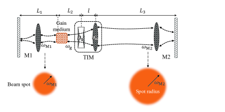
Figure 6: Diagram of the SSR ($\omega_{\mathrm{M1}},~{}\omega_{\mathrm{M2}},~{}\omega_{\mathrm{g}}$: beam spot radius; $L_{1}\sim L_{3}$: elements’ distance; M1, M2: retor-reflectors; $D_{1},~{}D_{2}$ lenses)

Taking the matrix elements from $\mathbf{M}_{\mathrm{RT}}$ into (14), the following inequality can be obtained as:

$$0< (\frac{f_{2}}{f_{1}}+\frac{l-(L_{1}+L_{2})\frac{f_{2}}{f_{1}}-\frac{L_{3}f_{1}}{f_{2}}}{f_{r1}})$$ (15)

$$\cdot(\frac{f_{1}}{f_{2}}+\frac{l-(L_{1}+L_{2})\frac{f_{2}}{f_{1}}-\frac{L_{3}f_{1}}{f_{2}}}{f_{r2}})<1,$$

where $f_{1}$ and $f_{2}$ express the focal length of lens $D_{1}$ and $D_{2}$; $f_{r1}$ and $f_{r2}$ express the $f_{r}$ parameter of retro-reflectors M1 and M2; $l,~{}L_{1},~{}L_{2},~{}L_{3}$ are distance parameters presenting in Fig. 6.

III-B Beam Spot Radius

From section II.C, we know that the beam loss may occur on the aperture, and a TIM is introduced in the transmission path to compress the incident beam distribution and inhibit the beam loss. In RB-SWIPT, the process of beam compression need and the change of beam distribution detail analysis.

Fig. 7 shows the schematic of the TIM and the process of the beam compression. The TIM is composed by a concave lens and a convex lens, and their focal length is $f_{1}$ and $f_{2}$. Two lenses are placed in parallel, and their focuses are overlap ($l=f_{1}+f_{2}$) [24]. When the resonant beam enters the TIM, it will first pass the convex lens. Under the function of the lens, the phase of the beam is changed, which makes the beam transmit toward the lens’s focal point. Then, the beam passes the concave lens, and a second phase change is undergone, which leads the beam parallelly emitting from the concave lens. Using the transmission matrix in Table I, the process can be expressed as:

$$\mathbf{M}_{D_{2}}\mathbf{M}_{l}\mathbf{M}_{D_{1}} =\left[\begin{array}[]{cc}1&0\\ -\frac{1}{f_{2}}&1\\ \end{array}\right]\left[\begin{array}[]{cc}1&l\\ 0&1\\ \end{array}\right]\left[\begin{array}[]{cc}1&0\\ -\frac{1}{f_{1}}&1\\ \end{array}\right]$$ (16)

$$=\left[\begin{array}[]{cc}\frac{1}{M}&l\\ 0&M\\ \end{array}\right],$$

where $M=-f_{2}/f_{1}$ is introduced as the TIM structure parameter.

We assume all optical elements involved have ideal optical properties, and the fundamental mode in resonant beams is dominant. Thus, we can use circular beam spot to define the beam distribution. Then, its radius can judge the beam’s change. According to (16), the TIM can convert the beam with spot radius from $\omega^{\prime}$ to $\omega^{\prime\prime}$ with convention relationship $\omega^{\prime\prime}=\omega^{\prime}/M$. In accordance with analysis presenting in Section II.C, gain medium usually has the smallest geometry which will produce the diffraction loss. Therefore, the TIM is set on the side of the gain medium close to the receiver.

In section III.A, we have developed the beam transmission matrix $\mathbf{M}_{\mathrm{RT}}$ which can depict the beam propagation in SSR. Based on it and theory in  [25], the spot radius of the beam on the gain medium $\omega_{g}$ can be depicted as:

$$\omega_{g}\approx\omega_{\mathrm{M1}}=\sqrt{\frac{\lambda}{\pi}\sqrt{\frac{\xi^{2}\zeta_{2}}{\zeta_{1}(1-\zeta_{1}\zeta_{2})}}},$$ (17)

where $\omega_{\mathrm{M1}}$ represent the spot radius of the beam on the M1 ($\omega_{g}\approx\omega_{\mathrm{M1}}$: considering the M1 and the gain medium are adjacent); $\lambda$ is the wavelength of the resonant beam; $\zeta_{1},~{}\zeta_{2}$, and $\xi$ are intermediate variables, which are defined as:

$${\color[rgb]{0,0,1}\left\{\begin{aligned} \zeta_{1}=&~{}-\frac{f_{2}}{f_{1}}-\frac{l-(L_{1}+L_{2})\frac{f_{2}}{f_{1}}-\frac{L_{3}f_{1}}{f_{2}}}{f_{r1}}\\ \zeta_{1}=&~{}-\frac{f_{1}}{f_{2}}-\frac{l-(L_{1}+L_{2})\frac{f_{2}}{f_{1}}-\frac{L_{3}f_{1}}{f_{2}}}{f_{r2}}\\ \xi=&~{}l-(L_{1}+L_{2})\frac{f_{2}}{f_{1}}-\frac{L_{3}f_{1}}{f_{2}}\end{aligned}\right..}$$ (18)

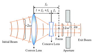
Figure 7: Beam compressed by TIM ($\omega$: initial beam radius; $\omega^{\prime}$: compressed beam radius; $a$: aperture radius; $f_{2}$: focal length of convex lens ($f_{2}>0$); $f_{1}$: focal length of concave lens ($f_{1}<0$); $l$ distance of two lenses)

Utilizing the (17), we can evaluate the change of beam distribution after it pass the TIM. Further, we can obtain the beam compression performance of the TIM.

III-C Energy harvesting and Data receiving

After the processes of energy-absorbing and stimulated radiation, the resonant beam generates and cyclically oscillate in the SSR. In the receiver, part of the beam will emission from the reflector M2 as a function of the external beam. Based on the cyclic power principle [21] and RB system structure presented in Section II, the external beam power can be defined as:

$$P_{\mathrm{beam}}=\eta_{s}(P_{\mathrm{in}}-P_{\mathrm{th}}),$$ (19)

where $\eta_{s}$ is the slope efficiency, $P_{\mathrm{in}}$ is the input power, and $P_{\mathrm{th}}$ is the threshold power (only $P_{\mathrm{in}}>P_{\mathrm{th}}$ the external beam can be output). The specific expression of $\eta_{s}$ and $P_{\mathrm{th}}$ are:

$$\left\{\begin{aligned} \eta_{s}=&\frac{2\eta_{c}(1-R_{2})}{(\delta_{c}-\ln R_{2})(1+R_{2})}\\ P_{\mathrm{th}}=&{\color[rgb]{0,0,1}\left(\frac{\delta_{c}-\ln R_{2}}{2}\right)\frac{A}{\eta_{c}}I_{s}}\end{aligned}\right.,$$ (20)

where $\eta_{c}=\eta_{p}\eta_{t}\eta_{a}\eta_{g}\eta_{B}$ expresses the compounded energy conversion efficiency making by pump source efficiency $\eta_{p}$, radiation transfer efficiency $\eta_{t}$, radiation absorption efficiency $\eta_{a}$, gain conversion efficiency $\eta_{g}$, and beam overlap efficiency $\eta_{B}$; $R_{2}$ is the reflectivity of reflector M2; $A$ is the stimulated emission cross-section; $I_{s}$ is the saturation intensity; $\delta_{c}=-\text{In}(V_{p}^{2}V_{t}^{2}R_{1})$ is the compounded cavity loss factor consisting of reflectivity of reflector M1 ($R_{1}$), compound passing loss $V_{p}$ (beam reflection and absorption loss occur on passing the lenses and the gain), and beam transmission loss $V_{t}$.

According to Section II.C, the transmission loss $V_{t}$ mainly comes from the beam diffraction loss produced on the aperture. To analyze the $V_{t}$, we can use the field calculation. However, the field calculation based on the Fresnel-Kirchhoff diffraction theory and Fox-Li method has high computational cost. Thus, we adopt an approximation calculation method using the transmission matrix [26], based on which $V_{T}$ can be described as :

$${\color[rgb]{0,0,1}V_{t}} {\color[rgb]{0,0,1}=1-\delta_{d}}$$ (21)

$$={\color[rgb]{0,0,1}1-\exp\left[-2\pi\frac{a^{2}}{\lambda\xi}\sqrt{\frac{\zeta_{1}\left(1-\zeta_{1}\zeta_{2}\right)}{\zeta_{2}}}\right]}$$

where $\delta_{d}$ expresses the beam diffraction loss ratio; $\lambda$ is the wavelength of the resonant beam; $a$ expresses the radius of the effective aperture, and $L_{3}$ is the end-to-end distance.

To achieve data and energy simultaneously, we utilize the beam splitter to divide the external beam into two streams. One stream is used for energy harvesting, while the other is used for data receiving.

1) Energy harvesting: Firstly, after passing the splitter, the beam will propagate through the optical waveguide arriving at the PV cell. Then, the PV cell collects the optical beam and converts them to electrical power by photoelectric conversion. This process can be defined as [27]:

$$\left\{\begin{aligned} &P_{p}=\mu P_{\mathrm{beam}},\\ &P_{\mathrm{Eout}}=a_{1}P_{p}+b_{1},\end{aligned}\right.$$ (22)

where and $\mu$ is the beam split ratio, $a_{1}$ and $b_{1}$ are the structure compound parameters of the PV cell involving the cells’ number, background temperature, absorption efficiency, etc.

2) Data receiving: Different from scheme using PV for data receiving, avalanche photodiode (APD) [28, 29] is applied for receiving the optical signal carried by the external beam, which can be expressed as:

$$P_{d}=(1-\mu)P_{\mathrm{beam}}.$$ (23)

To describe the process of data receiving on APD, we introduce the additive white Gaussian noise (AWGN). The shot noise and thermal noise are involved in the AWGN, which satisfies the following relationship as:

$$n_{t}^{2}=n^{2}_{\mathrm{shot}}+n^{2}_{\mathrm{thermal}},$$ (24)

where the $n_{\mathrm{thermal}}$ and $n_{\mathrm{shot}}$ are expressed thermal noise and shot noise. Among them, the shot noise can be expressed as [30]:

$$n^{2}_{\mathrm{shot}}=2q(\gamma P_{d}+I_{\mathrm{bg}})B_{x},$$ (25)

where $q$ is the electron charge, $B_{x}$ is the bandwidth of APD, $I_{bg}$ is the background current. Then, the thermal noise can be defined as [30]:

$$n^{2}_{\mathrm{thermal}}=\frac{4KTB_{x}}{R_{L}},$$ (26)

where $K$ is the Boltzmann constant, $T$ is the background temperature, and $R_{L}$ is the load resistor. At this time, the spectral efficiency (throughput) of the system can be described as [31]:

$${\color[rgb]{0,0,1}\widetilde{C}=\frac{1}{2}\log_{2}\left(1+\frac{(\gamma P_{d})^{2}}{2\pi\mathrm{e}n^{2}_{t}}\right),}$$ (27)

where $\mathrm{e}$ is the natural constant, $n_{t}^{2}$ is the noise power, and $\gamma$ is the parameter of the optical-to-electrical conversion responsivity of APD. Further, the signal-to-noise ratio (SNR) can also obtain, which is:

$${\color[rgb]{0,0,1}\mathrm{SNR}_{\mathrm{dB}}=10\log_{10}\left(\frac{(\gamma P_{d})^{2}}{n_{t}^{2}}\right).}$$ (28)

IV Numerical Analysis

In this section, to evaluate the ability of the RB-SWIPT system, we will compare the transmission performance of it to the original systems at first. Then, we will analyze the impact of structure parameters on the transmission distance, diffraction loss, output power and data transfer, giving the achievable performance of the RB-SWIPT system.

IV-A Performance Comparison

According to Section III.B, we can use the beam spot radius to analyze the beam’s changing, and the external beam power to analyze the end-to-end energy transmission performance. Besides, we will adopt some constant parameters from [14, 21] as the typical SSR parameters.

1) Beam spot radius: We set the distance of M1 and gain medium $L_{1}=4$ cm. The gain medium and TIM are adjacent ($L_{2}=1$ cm), considering the integration of elements in the transmitter. The $f_{r}$ parameter of M1 takes $f_{r2}=\infty$ ($d=f$). The $f_{r}$ parameter of M2 takes $f_{r2}=10$ m. The geometric radius of gain is 1 mm. The focal length of $D_{1}$ takes $f_{1}=-10$ mm. The TIM’s parameter takes $M=3$, and the wavelength of beam is 1064 nm. Adopting these parameters into the models presented in Section III, the relationship of the spot radius on the gain medium $\omega_{g}$ and end-to-end distance $L_{3}$ is given in Fig. 8 (blue curves). As can be seen, the beam spot radius of the proposed system with the TIM can keep less than 0.4 mm, while the beam spot radius of the original system without TIM (M=1) is more than 0.5 mm. Moreover, as the values of $L_{3}$ increases, the $\omega_{g}$ of proposed scheme changes smoothly, while the beam spot radius of the original scheme will drastically increase to 1.3 mm ($>$1 mm). Overall, numerical results show that the proposed scheme can efficiently compress the incident beam on gain medium, and sustain the compression condition in a variety of ranges.

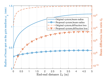
Figure 8: Beam spot radius and diffraction loss on gain medium versus end-to-end distance

2) Diffraction loss: Furthermore, using parameters defined above and setting $M=1$ and $M=3$ as the reference point, we obtain the relationship curves of the diffraction loss producing on the gain medium $\delta_{d}$ and the end-to-end transmission distance $L_{3}$. According to Fig. 8 red curves, both the $\delta_{d}$ of the proposed system ($M=3$) and original system ($M=1$) will increase as the $L_{3}$ increasing. However, the diffraction loss in the proposed system is close to 0 ($<10^{-4}$), which proves the diffraction loss is effectively reduced through the beam compression. In contrast, the $\delta_{d}$ of the original increases to 0.3 at $L_{3}$ = 5 m, presenting a high power attenuation.

In summary, compared with the original system, the proposed system can achieve effective and steady beam-compression, which prominently restrain the diffraction loss in long-range beam transmission.

IV-B Achievable Performance of RB-SWIPT System

In this part, we will further evaluate the achievable performance of the RB-SWIPT system. The obtained relationship between system performance and parameters has guiding value for system design and optimization.

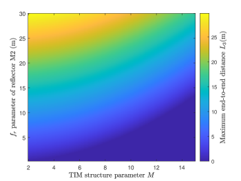
Figure 9: Maximum end-to-end distance intensity distribution on different $f_{r2}$ and $M$

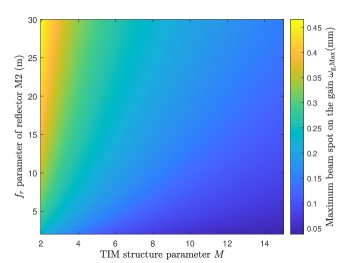
Figure 10: Maximum spot radius of beam on the gain medium intensity distribution on different $M$ and $f_{r2}$

1) Stable transmission distance: According to Section III.A, resonator stability is the prerequisite for system operation, which ensures the beam oscillation between the receiver and the transmitter.

We can get the maximum stable transmission distance through the inequality (15). Firstly, considering some parameters are constant, we mainly evaluate the impact of $M$ and $f_{r2}$ on the system performance. Then, based on the parameters’ value set in the above section and comprehensively considered the influence of the two parameters on $L_{\mathrm{3,Max}}$, the relationship between curvature radius $f_{r2}$, TIM’s structure parameter $M$, and the maximum end-to-end transmission distance $L_{\mathrm{3,Max}}$ as the intensity distribution diagram can be depicted in Fig. 9. As can be seen, both the $M$ and $f_{r2}$ impact the $L_{\mathrm{3,Max}}$. When $f_{r2}$ is fixed, to achieve a large $L_{\mathrm{3,Max}}$, $M$ needs to take a large value. In accordance with the model in Section II.A, $f_{1}$ and $f_{2}$ are the focal length of TIM’s lenses, which influence the optical capability of the TIM. Thus, the change of $M=-f_{2}/f_{1}$ will impact $L_{\mathrm{3,Max}}$. In numerical, $L_{\mathrm{3,Max}}$ can be 25 m when $M$ takes 2$\sim$10 and $f_{r2}$ takes 20$\sim$30 m. Overall, $L_{\mathrm{3,Max}}$ presents a positive increase relationship with $f_{r2}$ and $M$. Thus, considering the resonator stability, $M$ and $f_{r2}$ need to design as a large value to support long-range SWIPT in practice.

2) Beam spot radius: Because of the beam divergence, the radius of beam spot will be different at different distances, we introduce the maximum value of the spot radius $\omega_{\mathrm{g,Max}}$on the gain medium to analyze. Based on (9), (17), Table I, and the parameters determined above, the relationship of $\omega_{\mathrm{g,Max}}$and $M$ can be obtained as the function of intensity variation presenting in Fig. 10. As can be seen, $M$ and $f_{r2}$ all have an effect on the $\omega_{\mathrm{g,Max}}$. When $f_{r2}$ is fixed, $L_{\mathrm{3,Max}}$ will decrease as $M$ increase, which indicates that the ability of beam compression gains. On the contrary, $f_{r2}$ has the positive impact on $L_{\mathrm{3,Max}}$. Numerically, $L_{\mathrm{3,Max}}$ can be 0.35$\sim$0.45 mm when $M$ takes 2$\sim$5 and $f_{r2}$ takes 10$\sim$30 m.

Generally, we can strengthen the compression capability by increase the parameter $M$ and reduce the $f_{r2}$.

3) Beam diffraction loss: In Section IV.A, we compare and analyze the beam diffraction loss on original system and the proposed system. In this part, we will further analyze the beam diffraction loss at different structure parameters.

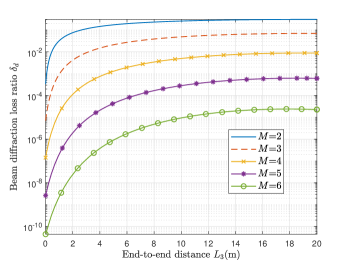
Figure 11: Beam diffraction loss ratio versus end-to-end distance at different $M$

Firstly, we enhance the transmission distance range to 20 m. Then, according to abovementioned analysis, we set the $f_{r2}=$40 m. Finally, taking the constant parameters defined above, the curves of the beam diffraction loss ratio $\delta_{d}$ as a function of transmission distance $L_{3}$ with different $M$ can be presented in Fig. 11. With the transmission distance increasing, the curves present a same trend that rising sharply at first and then being flat. Moreover, with the $M$ being large, the curves will move down, which means the value of $\delta_{d}$ will become smaller when $M$ becomes larger. In numerical, values of $\delta_{d}$ are distributed between $10^{-10}$ and $10^{-1}$. Overall, we can design appropriate $M$ to keep $\delta_{d}$ close to 0 over long-range transmission.

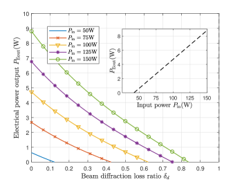
Figure 12: Output electrical power versus beam diffraction loss at different input power; output electrical power versus input power ($\delta_{d}\approx 0$)

4) Energy harvesting: To evaluate the performance of the energy harvesting, we set the $\mu$ =1 to test the charging performance that all the external beam energy deliver to PV.

The system boundary parameters need to be defined. Firstly, the reflectivity of M1 and M2 are set as 0.999 and 0.2618. $a_{1}$ and $b_{1}$ of the PV cell are taken 0.3487 and -1.525 [14]. Then, we take the value of pump source efficiency $\eta_{p}=0.5$, the radiation transfer efficiency $\eta_{t}=0.98$, the radiation absorption efficiency $\eta_{a}=0.85$, the gain conversion efficiency $\eta_{g}=0.72$, the beam overlap efficiency $\eta_{B}=0.95$, and the compound passing loss $V_{p}=0.96$ [21]. Finally, we define the saturation intensity of gain medium (Nd:YV$\mathrm{O_{4}}$) $I_{s}=1.1976\times 10^{7}$ W/$m^{2}$, and the stimulated emission cross-section A = 7.8540$\times 10^{-7}~{}\mathrm{m^{2}}$.

We use different $P_{\mathrm{in}}$ as reference point and the constant boundary parameters defined above. The relationship between the output power $P_{\mathrm{out}}$ and beam diffraction loss ratio $\delta_{d}$ can be obtained. As shown in Fig. 12, with the increase of $\delta_{d}$, the values of $P_{\mathrm{Eout}}$ will quickly drop to 0 with a downward linear trend. Moreover, when $P_{\mathrm{in}}$ takes a large value, the entire curves of $P_{\mathrm{Eout}}$ will move up, presenting a higher power output (7$\sim$9 W). Besides, we depict the line of the $P_{\mathrm{Eout}}$ as the function of $P_{\mathrm{in}}$ when the $\delta_{d}\approx 0$ for simulating the situation that the TIM is applied. From Fig. 12 subgraph, $P_{\mathrm{Eout}}$ and $P_{\mathrm{in}}$ present a positive linear relationship. Numerically, the threshold power of the system is around 40 W. $P_{\mathrm{Eout}}$ can be 0$\sim$9 W when the value of $P_{\mathrm{in}}$ takes 0$\sim$150 W.

TABLE II: Comparison of existing SWIPT schemes

Schemes&Authors	Input Power	Output power	Spectral efficiency	Transmission Distance
RF-based; Krikidis $et~{}al.$ [32]	10$\mathrm{~{}W}$	5$\mathrm{~{}mW}$	7 $\mathrm{bit/s}/\mathrm{Hz}$	10$\mathrm{~{}m}$
RF-based; Lu $et~{}al.$ [33]	4$\mathrm{~{}W}$	5.5$\mathrm{~{}\mu W}$	not stated	15$\mathrm{~{}m}$
VL-based; Ma $et~{}al.$ [34]	316.2$\mathrm{~{}W}$	2.96$\mathrm{~{}mW}$	6 $\mathrm{bit/s}/\mathrm{Hz}$	1.5$\mathrm{~{}m}$
VL-based; Abdelhady $et~{}al.$ [35]	450$\mathrm{~{}W}$	0.38$\mathrm{~{}mW}$	8 $\mathrm{bit/s}/\mathrm{Hz}$	3.0$\mathrm{~{}m}$
This work	150$\mathrm{~{}W}$	9 W	20 bit/s/Hz	18$\mathrm{~{}m}$

4) Data receiving: Firstly, we take optical-to-electrical conversion responsivity of APD $\gamma$ = 0.6 A/W [36], the bandwidth of the noise $B_{x}$ = 811.7 MHz [37], the electron charge $q$ = $1.6\times 10^{-19}$ C, the background current $I_{bg}$ = 5100 $\mu A$ [38], the Boltzmann constant $K$ = $1.38\times 10^{-23}$ J/K, the background temperature $T$ = 300 K, and load resistor $R_{L}$ = 10 K$\Omega$ [30]. Then, we set the input power $P_{\mathrm{in}}$ = 80 W as reference point. Finally, applying these parameters into (23)-(28), the relationship between the spectral efficiency $\widetilde{C}$, SNR, and beam split ratio $\mu$ can be described in Fig. 13. As is shown, the spectral efficiency of the proposed system can be 20 bit/s/Hz, and the SNR is greater than 100 dB, which shows a remarkable data transfer capability. With the $\mu$ increasing, both the spectral efficiency and SNR show a slow downward trend before the $\mu$ is close to 0. It proves that the APD has a great sensitivity for data receiving, and small values of $1-\mu$ can be taken. Moreover, we also put the relationship of the SNR and spectral efficiency. As in Fig. 13 subgraph, the SNR and spectral efficiency present a liner relationship. A great spectral efficiency needs the SNR to take a high value.

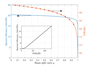
Figure 13: Beam split ratio $\mu$ versus spectral efficiency and SNR; spectral efficiency versus SNR

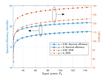
Figure 14: Spectral efficiency and SNR versus input power

To explore the impact of input power on spectral efficiency and SNR, we set the split $\mu$ = 0.95 and 0 as reference points, and take input power $P_{\mathrm{in}}$ 0 to 140W. After the parameters substitution and formula calculation, the relationship curves of input power, spectral efficiency and SNR can be obtained in Fig. 14. As is presented, with $P_{\mathrm{in}}$ increasing, curves of the spectral efficiency and SNR will rise slowly. When $\mu$ equals to 0 (all beam is assigned to APD), both the spectral efficiency and SNR enhance. Numerically, the spectral efficiency increases near 2 bit/s/Hz, while the SNR promotes 10 dB. These results prove that high input signal power benefits the data transfer. However, the amount of increase that can be made is restricted. In practice, $\mu=0.95$ can achieve 18 bit/s/Hz spectral efficiency and 120 dB SNR, which makes the system has the capability to supply high quality data transfer and high power output.

IV-C Summary

After numerical evaluation and analysis, we can make a summary that the suggested RB-SWIPT system can effectively restrain the transmission loss caused by beam diffraction to near 0 over a distance of 20 m. Moreover, the system can support 0$\sim$9 W electrical power for charging and a maximum spectral efficiency of 20 bit/s/Hz for data transfer. Table II compares the performance of our scheme to the typical SWIPT designs such as visible light (light-emitting diode as beam source) SWIPT and radio frequency SWIPT. As can be seen, the proposed RB-SWIPT has advantages in high power charginh while also supporting high spectral efficiency for communication over long distance.

V Discussion

V-A Spherical Aberration

According to Fig. 6, there are various optical lenses with spherical surfaces in the system, which are adopted for beam modulation. Ideally, light beam passes through these lenses converge or diverge to a point along the desired par-axial path. If it passes through a lens deviating from the ideal point, spherical aberration will produce  [39]. The existence of spherical aberration affects the end-to-end transmission of beam and makes the quality of beam deteriorate [40, 39, 41].

Figure 15: Spherical aberration

Fig. 15 depicts the spherical aberration. As can be seen, light rays can converge to the focal point when passing through an ideal lens. On the contrary, part of the rays are out of focus in normal lens.

In this paper, we assume that the involved lenses have ideally optical characteristic and the resonant beam is fundamental mode (with the ideal beam quality). If the normal lenses are adopted, the multimode beam will exist in resonator and the system performance will inevitably differ from the simulation results. According to [15], when the system uses normal lenses with large spherical aberration, over 70$\%$ of the energy may lose. Therefore, the actual system performance may be worse than the numerical results. To ensure the beam transmission efficiency, the system needs to suppress spherical aberration. The combination of positive and negative lenses and using aspheric lenses are two typical schemes to remove spherical aberration [39, 42]. Specifically, the spherical aberration of a positive lens is negative, and that of a negative lens is negative. Therefore, the combination of positive and negative lenses can effectively suppress the spherical aberration. Aspheric lens technology adopts changing the shape of the lens surface and adjusting the curvature of some positions, the global spherical aberration of the lens can be eliminated. In future work, a detailed analysis and evaluation about the spherical aberration will be presented, independently.

VI Conclusions

A long-range optical wireless information and power transfer scheme is proposed in this paper. The scheme utilize retro-reflectors, a gain medium, a telescope internal modulator forming the resonant beam, which can realize high-power charging and high-rate communication. An analytical model of the scheme has been developed to evaluate resonator stability, transmission loss, beam distribution, energy harvesting, and data receiving. The impact of structure parameters on system performance has been analyzed. A discussion of spherical aberration has been conduct. Numerical results illustrate that the proposed scheme can support 0$\sim$9 W power and enable 18 bit/s/Hz spectral efficiencies simultaneously over 20 m.

References

- [1] R. Zhang and C. K. Ho, “MIMO broadcasting for simultaneous wireless information and power transfer,” IEEE Transactions on Wireless Communications, vol. 12, no. 5, pp. 1989–2001, Mar. 2013.
- [2] K. Georgiou, S. Xavier-de Souza, and K. Eder, “The IoT energy challenge: A software perspective,” IEEE Embedded Systems Letters, vol. 10, no. 3, pp. 53–56, Jun. 2017.
- [3] K. David and H. Berndt, “6G Vision and Requirements: Is There Any Need for Beyond 5G?” IEEE Vehicular Technology Magazine, vol. 13, no. 3, pp. 72–80, July. 2018.
- [4] M. S. Bahbahani and E. Alsusa, “A cooperative clustering protocol with duty cycling for energy harvesting enabled wireless sensor networks,” IEEE Transactions on Wireless Communications, vol. 17, no. 1, pp. 101–111, Jan. 2018.
- [5] K. Wang, Y. Wang, Y. Sun, S. Guo, and J. Wu, “Green industrial internet of things architecture: An energy-efficient perspective,” IEEE Communications Magazine, vol. 54, no. 12, pp. 48–54, Dec. 2016.
- [6] K. Huang and E. Larsson, “Simultaneous information and power transfer for broadband wireless systems,” IEEE Transactions on Signal Processing, vol. 61, no. 23, pp. 5972–5986, Dec 2013.
- [7] N. Shinohara, Wireless power transfer via radiowaves. Wiley Online Library, 2014.
- [8] H. Haken, “Laser theory,” in Light and Matter Ic/Licht und Materie Ic. Springer, 1970, pp. 1–304.
- [9] M. Liu, H. Deng, Q. Liu, J. Zhou, M. Xiong, L. Yang, and G. B. Giannakis, “Simultaneous mobile information and power transfer by resonant beam,” IEEE Transactions on Signal Processing, pp. 1–1, May 2021.
- [10] M. A. Khalighi and M. Uysal, “Survey on free space optical communication: A communication theory perspective,” IEEE communications surveys & tutorials, vol. 16, no. 4, pp. 2231–2258, 2014.
- [11] W. Chen, S. Zhao, Q. Shi, and R. Zhang, “Resonant beam charging-powered UAV-assisted sensing data collection,” IEEE Transactions on Vehicular Technology, pp. 1–1, Oct. 2019.
- [12] A. Ortal, Z. Nes, P. Rudiger, and Zurich, “Wireless laser system for power transmission utilizing a gain medium between retroreflectors,” U.S. Patent 9 653 949, May 16, 2017.
- [13] Q. Zhang, W. Fang, Q. Liu, J. Wu, P. Xia, and L. Yang, “Distributed laser charging: A wireless power transfer approach,” IEEE Internet of Things Journal, vol. 5, no. 5, pp. 3853–3864, Oct. 2018.
- [14] W. Wang, Q. Zhang, H. Lin, M. Liu, X. Liang, and Q. Liu, “Wireless energy transmission channel modeling in resonant beam charging for IoT devices,” IEEE Internet of Things Journal, vol. 6, no. 2, pp. 3976–3986, Apr. 2019.
- [15] Q. Sheng, M. Wang, H. Ma, Y. Qi, J. Liu, D. Xu, W. Shi, and J. Yao, “Continuous-wave long-distributed-cavity laser using cat-eye retroreflectors,” Opt. Express, vol. 29, no. 21, pp. 34 269–34 277, Oct. 2021.
- [16] Q. Sheng, A. Wang, M. Wang, H. Ma, Y. Qi, J. Liu, S. Wang, D. Xu, W. Shi, and J. Yao, “Enhancing the field of view of a distributed-cavity laser incorporating cat-eye optics by compensating the field-curvature,” Optics Laser Technology, vol. 151, p. 108011, Feb. 2022.
- [17] M. Xiong, Q. Liu, M. Liu, and P. Xia, “Resonant beam communications,” in ICC 2019 - 2019 IEEE International Conference on Communications (ICC), May 2019, pp. 1–6.
- [18] M. Xiong, M. Liu, Q. Jiang, J. Zhou, Q. Liu, and H. Deng, “Retro-reflective beam communications with spatially separated laser resonator,” IEEE Transactions on Wireless Communications, vol. 20, no. 8, pp. 4917–4928, Mar. 2021.
- [19] A. Al-Kinani, C.-X. Wang, L. Zhou, and W. Zhang, “Optical wireless communication channel measurements and models,” IEEE Communications Surveys & Tutorials, vol. 20, no. 3, pp. 1939–1962, May. 2018.
- [20] M. Eichhorn, Laser physics: from principles to practical work in the lab. Springer Science & Business Media, 2014.
- [21] W. Koechner, Solid-state laser engineering. Springer, 2013, vol. 1.
- [22] R. N. N. Hodgson and I. H. Weber, Laser Resonators and Beam Propagation. Springer, 2005, vol. 108.
- [23] H. Kogelnik and T. Li, “Laser beams and resonators,” Appl. Opt., vol. 5, no. 10, pp. 1550–1567, Oct. 1966.
- [24] M. Born and E. Wolf, Principles of optics: electromagnetic theory of propagation, interference and diffraction of light. Elsevier, 2013.
- [25] P. Baues, “Huygens’ principle in inhomogeneous, isotropic media and a general integral equation applicable to optical resonators,” Opto-electronics, vol. 1, no. 1, pp. 37–44, Feb. 1969.
- [26] S. Cao, S. Tu, Y. Huang, H. Fan, J. Li, H. Xia, and G. Ren, “Analysis of diffraction loss in laser resonator,” Laser Technol., vol. 42, no. 3, pp. 400–403, May. 2018.
- [27] Q. Zhang, W. Fang, M. Xiong, Q. Liu, J. Wu, and P. Xia, “Adaptive resonant beam charging for intelligent wireless power transfer,” IEEE Internet of Things Journal, vol. 6, no. 1, pp. 1160–1172, Feb. 2018.
- [28] M. S. Aziz, S. Ahmad, I. Husnain, A. Hassan, and U. Saleem, “Simulation and experimental investigation of the characteristics of a pv-harvester under different conditions,” in 2014 International Conference on Energy Systems and Policies (ICESP). IEEE, 2014, pp. 1–8.
- [29] J. C. Campbell, “Recent advances in telecommunications avalanche photodiodes,” Journal of Lightwave Technology, vol. 25, no. 1, pp. 109–121, Jan. 2007.
- [30] F. Xu, M. Khalighi, and S. Bourennane, “Impact of different noise sources on the performance of pin- and apd-based fso receivers,” in Proceedings of the 11th International Conference on Telecommunications, Jun. 2011, pp. 211–218.
- [31] A. Lapidoth, S. M. Moser, and M. A. Wigger, “On the capacity of free-space optical intensity channels,” IEEE Transactions on Information Theory, vol. 55, no. 10, pp. 4449–4461, Oct. 2009.
- [32] I. Krikidis, S. Timotheou, S. Nikolaou, G. Zheng, D. W. K. Ng, and R. Schober, “Simultaneous wireless information and power transfer in modern communication systems,” IEEE Communications Magazine, vol. 52, no. 11, pp. 104–110, Nov. 2014.
- [33] X. Lu, P. Wang, D. Niyato, and E. Hossain, “Dynamic spectrum access in cognitive radio networks with rf energy harvesting,” IEEE Wireless Communications, vol. 21, no. 3, pp. 102–110, Jun. 2014.
- [34] S. Ma, F. Zhang, H. Li, F. Zhou, Y. Wang, and S. Li, “Simultaneous lightwave information and power transfer in visible light communication systems,” IEEE Transactions on Wireless Communications, vol. 18, no. 12, pp. 5818–5830, Dec. 2019.
- [35] A. M. Abdelhady, O. Amin, B. Shihada, and M.-S. Alouini, “Spectral efficiency and energy harvesting in multi-cell slipt systems,” IEEE Transactions on Wireless Communications, vol. 19, no. 5, pp. 3304–3318, Feb. 2020.
- [36] M. S. Demir, F. Miramirkhani, and M. Uysal, “Handover in vlc networks with coordinated multipoint transmission,” in 2017 IEEE International Black Sea Conference on Communications and Networking (BlackSeaCom), Jun. 2017, pp. 1–5.
- [37] C. Quintana, Q. Wang, D. Jakonis, X. Piao, G. Erry, D. Platt, Y. Thueux, A. Gomez, G. Faulkner, H. Chun, M. Salter, and D. O’Brien, “High speed electro-absorption modulator for long range retroreflective free space optics,” IEEE Photonics Technology Letters, vol. 29, no. 9, pp. 707–710, Mar. 2017.
- [38] A. J. Moreira, R. T. Valadas, and A. de Oliveira Duarte, “Optical interference produced by artificial light,” Wireless Networks, vol. 3, no. 2, pp. 131–140, May. 1997.
- [39] Spherical aberration. [Online]. Available: https://en.wikipedia.org/wiki/Spherical_aberration
- [40] Q. Sheng, A. Wang, Y. Ma, S. Wang, M. Wang, Z. Shi, J. Liu, S. Fu, W. Shi, J. Yao et al., “Intracavity spherical aberration for selective generation of single-transverse-mode laguerre-gaussian output with order up to 95,” PhotoniX, vol. 3, no. 1, pp. 1–12, Feb. 2022.
- [41] M. Wang, Y. Ma, Q. Sheng, X. He, J. Liu, W. Shi, J. Yao, and T. Omatsu, “Laguerre-gaussian beam generation via enhanced intracavity spherical aberration,” Optics Express, vol. 29, no. 17, pp. 27 783–27 790, Aug. 2021.
- [42] J. Liu, A. Wang, Q. Sheng, Y. Qi, S. Wang, M. Wang, D. Xu, S. Fu, W. Shi, and J. Yao, “Large-range alignment-free distributed-cavity laser based on an improved multi-lens retroreflector,” Chinese Optics Letters, vol. 20, no. 3, p. 031407, Dec. 2022.