A More Precise Mass for GJ 1214 b and the Frequency of Multi-Planet Systems Around Mid-M Dwarfs

Abstract

We present an intensive effort to refine the mass and orbit of the enveloped terrestrial planet GJ 1214 b using 165 radial velocity (RV) measurements taken with the HARPS spectrograph over a period of ten years. We conduct a joint analysis of the RVs with archival Spitzer/IRAC transits and measure a planetary mass and radius of $8.17\pm 0.43$ $M_{\oplus}$ and $2.742^{+0.050}_{-0.053}$ $R_{\oplus}$. Assuming GJ 1214 b is an Earth-like core surrounded by a H/He envelope, we measure an envelope mass fraction of $X_{\rm env}=$ $5.24^{+0.30}_{-0.29}$%. GJ 1214 b remains a prime target for secondary eclipse observations of an enveloped terrestrial, the scheduling of which benefits from our tight constraint on the orbital eccentricity of $<$ $0.063$ at 95% confidence, which narrows the secondary eclipse window to 2.8 hours. By combining GJ 1214 with other mid-M dwarf transiting systems with intensive RV follow-up, we calculate the frequency of mid-M dwarf planetary systems with multiple small planets and find that $90^{+5}_{-21}$% of mid-M dwarfs with a known planet with mass $\in[1,10]$ $M_{\oplus}$ and orbital period $\in[0.5,50]$ days, will host at least one additional planet. We rule out additional planets around GJ 1214 down to 3 $M_{\oplus}$ within 10 days such that GJ 1214 is a single-planet system within these limits, a result that has a $44^{+9}_{-5}$% probability given the prevalence of multi-planet systems around mid-M dwarfs. We also investigate mid-M dwarf RV systems and show that the probability that all reported RV planet candidates are real planets is $<12$% at 99% confidence, although this statistical argument is unable to identify the probable false positives.

1 Introduction

GJ 1214 remains a benchmark system for M dwarf planetary systems with small planets in the super-Earth to sub-Neptune size regime (Charbonneau et al., 2009). The accessibility of the GJ 1214 system for detailed characterization has warranted measurements of spectroscopic stellar parameters (Anglada-Escudé et al., 2013a), photometric variability studies (Berta et al., 2011; Narita et al., 2013; Nascimbeni et al., 2015), and X-ray activity monitoring (Lalitha et al., 2014). The planet GJ 1214 b itself has been subject to a multitude of searches for transit timing variations (TTV) (Carter et al., 2011; Harpsøe et al., 2013; Fraine et al., 2013; Gillon et al., 2014) and atmospheric characterization efforts (Bean et al., 2011; Croll et al., 2011; Crossfield et al., 2011; de Mooij et al., 2012; Fraine et al., 2013; Kreidberg et al., 2014). The TTV searches have sought to 1) scrutinize the multiplicity of the inner planetary system, and 2) to improve constraints on the mass of GJ 1214 b if a second transiting planet was uncovered. These searches yielded null results and consequently were unable to provide an independent mass measurement of GJ 1214 b. Years of follow-up campaigns have generated the consensus that GJ 1214 is an inactive mid-M dwarf that hosts a single known planet, and given the radial velocity (RV) mass and radius of GJ 1214 b ($m_{p}=6.26\pm 0.91$ $M_{\oplus}$; Anglada-Escudé et al. 2013a, $2.85\pm 0.2$ $R_{\oplus}$; Harpsøe et al. 2013), the planet must be enveloped in H/He gas, although high-altitude clouds hinder the detection of chemical species in the deep atmosphere (Kreidberg et al., 2014).

The null results from the aforementioned TTV searches and the absence of additional RV measurements analyzed since the planet’s discovery implies that the mass of GJ 1214 b has not been refined since its discovery. Anglada-Escudé et al. (2013a) did however conduct a stellar plus RV analysis using the same RV data from the discovery paper (Charbonneau et al., 2009). Anglada-Escudé et al. (2013a) performed an independent RV extraction using the TERRA template-matching algorithm (Anglada-Escudé & Butler, 2012) and recovered a consistent RV semiamplitude with an equivalent measurement uncertainty of $\pm 1.6$ m s^-1.

In this study, we analyze the ten years of intensive RV follow-up of GJ 1214 with the aim to improve our understanding of the mass and orbital solution of GJ 1214 b and to search for additional planetary signals in the RV data. With these RV data, GJ 1214 joins the set of mid-M dwarfs with sufficient RV observations to be sensitive to the detection of additional sub-Neptune-mass planets within the system. By analyzing the RV sensitivity of GJ 1214 along with other mid-M dwarf planetary systems with comparable RV follow-up datasets, we present the frequency of mid-M dwarf planetary systems with multiple small planets with masses between 1-10 $M_{\oplus}$ and with orbital periods between 0.5-50 days.

In Section 2 we report the adopted stellar parameters. In Section 3 we present the RV and transit observations used in this study. In Section 4 we jointly model the RV and transit data to measure the mass and orbit of GJ 1214 b. In Section 5 we derive the RV sensitivity and place constraints on the presence of additional planets orbiting GJ 1214. In Section 6 we compute the frequency the multi-planet systems orbiting mid-M dwarfs. We conclude with a summary of our results in Section 7.

2 Stellar Parameters

GJ 1214 is a metal-rich M4 dwarf ([Fe/H]$=0.29\pm 0.12$ dex; Newton et al. 2014) located at a distance of $14.631\pm 0.012$ pc (Lindegren et al., 2021; Bailer-Jones et al., 2021). We use the star’s absolute $K_{s}$-band magnitude ($M_{K}=7.956\pm 0.020$) and metallicity to infer its stellar mass ($M_{s}=0.178\pm 0.010$ $M_{\odot}$) and radius ($R_{s}=0.215\pm 0.008$ $R_{\odot}$) using the empirical M dwarf mass-luminosity and radius-luminosity relations from Benedict et al. (2016) and Mann et al. (2015), respectively. We adopt the stellar effective temperature from Anglada-Escudé et al. (2013a), which derived $T_{\text{eff}}$ via SED fitting to the absolute $BVRIJHK_{s}$W1W2W3W4 magnitudes. The resulting value of $T_{\text{eff}}$ $=3250\pm 100$ K is in good agreement with the values derived from $K$-band water absorption (Rojas-Ayala et al., 2012) and from empirical temperature-color relations (Mann et al., 2015). The stellar luminosity, density, and surface gravity are derived self-consistently from the aforementioned parameters. The stellar parameters adopted throughout this work are summarized in Table 1.

Table 1: GJ 1214 physical stellar parameters.

Parameter	Value	Ref
GJ 1214, TIC 467929202,
Gaia DR3 4393265392168829056
Spectral type	M4	1
Stellar mass, $M_{s}$ [$M_{\odot}$]	$0.178\pm 0.010$	2
Stellar radius, $R_{s}$ [$R_{\odot}$]	$0.215\pm 0.008$	2
Stellar density, $\rho_{s}$ [g cm-3]	$25.4^{+3.5}_{-3.0}$	2
Stellar luminosity, $L_{s}$ [L⊙]	$0.0046^{+0.0007}_{-0.0006}$	2
Effective temperature, $T_{\text{eff}}$ [K]	$3250\pm 100$	3
Surface gravity, $\log{g}$ [dex]	$5.026\pm 0.040$	2
Metallicity, [Fe/H] [dex]	$0.29\pm 0.12$	1

Note. — References: 1) Newton et al. 2014 2) this work 3) Anglada-Escudé et al. 2013a.

3 Observations

3.1 HARPS Radial Velocities

GJ 1214 b was observed with the High Accuracy Radial velocity Planet Searcher (HARPS; Mayor et al., 2003) échelle spectrograph mounted at the 3.6m ESO telescope at La Silla Observatory, Chile. A total of 168 spectra were taken between UT 2009 June 11 and UT 2019 September 2, although we exclude three spectra with exceptionally low S/N (i.e. total S/N $<5$). Included in the remaining set of 165 spectra are the 21 RV observations originally published in the discovery paper of GJ 1214 b (Charbonneau et al., 2009) and subsequently reanalyzed by Anglada-Escudé et al. (2013a). The observations were obtained through five time allocations: ESO programs 183.C-0972, 283.C-5022 (P.I. Udry), and 1102.C-0339, 183.C-0437, 198.C-0838 (P.I. Bonfils). The exposure time was set to 2400 seconds in each program. Due to the low flux of the target spectrum, the simultaneous cailbration fiber was set to on-sky rather than to the standard thorium argon lamp to avoid any potential contamination of the lamp into the science fiber at the bluest échelle orders. A majority of the spectra were also read in the HARPS slow mode in order to minimize the read-out noise. In the first two observing programs (22/165 observations), we obtained a median S/N at the center of the order 66 ($\sim 650$ nm) of 18.8, which corresponds to a median RV uncertainty of 2.35 m s^-1. In the remaining ESO programs 1102.C-0339 (10/165 observations), 183.C-0437 (68/165 observations), and 198.C-0838 (65/165 observations), median S/N values at 650 nm of 13.9, 16.6, and 16.2, respectively, were obtained. The corresponding median RV uncertainties were 3.81, 3.35, and 3.25 m s^-1.

To achieve the RV uncertainties quoted above, we extracted each spectrum’s RV using the TERRA pipeline (Anglada-Escudé & Butler, 2012). TERRA employs a template-matching scheme which has been shown to produce an improved RV measurement precision on M dwarfs compared to the cross-correlation function (CCF) technique (e.g. Anglada-Escudé & Butler, 2012; Astudillo-Defru et al., 2015), which is employed by the HARPS Data Reduction Software (DRS; Lovis & Pepe, 2007). TERRA constructs an empirical, high S/N template spectrum by coadding the individual spectra after shifting to the solar system barycentric reference frame using the barycentric corrections calculated by the HARPS DRS. Spectral regions with telluric absorption exceeding 1% are omitted from the RV extraction process. Each spectrum’s RV is extracted via a linear least squares fit to the master template in velocity space. In our analysis, we ignore the bluest orders at low S/N and only consider spectral orders redward of order number 139 (440-687 nm).

In June 2015 (BJD = 2457176.5), the HARPS fiber link was upgraded to improve the instrument’s throughput, stability, and the uniformity of the emergent illumination pattern (Lo Curto et al., 2015). These improvements enhanced the RV stability of the instrument but produced a velocity offset that we account for in the RV extraction by constructing two template spectra for the subsets of data corresponding to pre and post-fiber upgrade (containing 90 and 75 out of 165 measurements, respectively). The resulting raw RV time series is provided in Table 2 and does not include corrections for the secular acceleration of GJ 1214, nor for any Rossiter-induced contamination of in-transit measurements. We find that six out of 165 of our RV measurements occur in-transit and may be marginally affected by the Rossiter-McLaughlin (RM) effect. Due to the slow rotation of GJ 1214, we can safely ignore this effect in our RV modeling as the expected RM signal amplitude is neglible compared to our typical RV uncertainties ($K_{\rm RM}\sim 1.1$ m s^-1; Gaudi & Winn, 2007) and in practice would appear smaller given that the exposure time is comparable to the transit duration.

Table 2: The raw HARPS RV time series of GJ 1214 in the solar system barycentric reference frame

Time	RV	$\sigma_{\text{RV}}$	Fiber Upgrade
$[$BJD - 2,450,000$]$	$[\text{m s}^{-1}]$	$[\text{m s}^{-1}]$	Status
4993.767485	-8.239	2.275	pre
7872.894813	-7.473	3.670	post

Note. — For conciseness, only a subset of rows are depicted here to illustrate the table’s contents. The entirety of this table is provided in the arXiv source code.

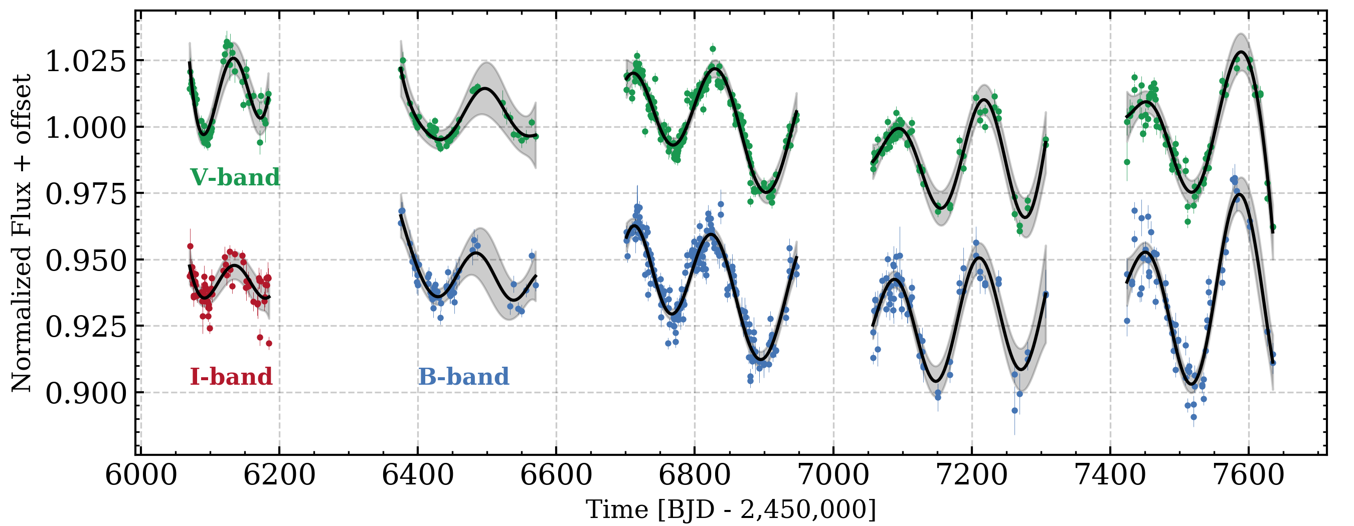
Figure 1: Long-term multi-color photometric monitoring of GJ 1214 with STELLA photometry. The blue, green, and red markers depict the $BVI$ light curves, respectively. The black curves depict the mean function of the quasi-periodic Gaussian process while the surrounding shaded region depicts its $3\sigma$ uncertainty.

3.2 Spitzer/IRAC Transit Photometry

Fraine et al. (2013) and Gillon et al. (2014) presented data from a continuous photometric monitoring program of GJ 1214 with the Spitzer Space Telescope. The program’s strategy and motivation were to monitor GJ 1214 for 20.9 days to characterize the infrared transit and secondary eclipse of GJ 1214 b, and to search for additional transiting planets down to Martian size out to the inner edge of the star’s habitable zone. These observations did not yield a significant detection of the secondary eclipse depth, nor did they yield any additional planet detections. However, these data provide us with high quality transit light curves that we will use in our global analysis of GJ 1214 b.

The data were taken with Spitzer’s Infrared Array Camera (IRAC; Fazio et al., 2004) as part of the Spitzer programs 542 (P.I. Desért) and 70049 (P.I. Deming). The observations feature three and fourteen transit observations at 3.6 and 4.5 µm, respectively. Gillon et al. (2014) also presented six secondary eclipse observations of GJ 1214 b that did not produce any significant detection of the eclipse depth. As such, we elect to omit the eclipse observations from our analysis and focus solely on the transit observations.

The Spitzer photometry contains apparent variations in flux due to intra-pixel sensitivity variations in the IRAC detectors. We corrected for this effect using the pixel-level decorrelation (PLD) method (Deming et al., 2015), implementing the procedure broadly as described by Garhart et al. (2020). We performed aperture photometry on all of the Spitzer data at both 3.6 and 4.5 µm, using eleven circular numerical apertures. The apertures had constant radii ranging from tightly centered on the point spread function (PSF), to much broader than the PSF (i.e. 1.6 to 3.5 pixels), and were centered on the stellar image using a 2-D Gaussian fit. We applied the PLD analysis to segments of the subsequent photometry, each segment having a span of approximately $\pm 3$ hours and centered on the predicted times of transit. In addition to fitting the photometry using the pixel coefficients (Deming et al., 2015), we also fit a quadratic baseline in time. There are two principal differences between our procedure and the analysis method described by Garhart et al. (2020). Firstly, we are fitting transits and not eclipses, so we include quadratic limb darkening using the values calculated for the Spitzer bandpasses (Claret et al., 2012). Secondly, at this phase we are interested only in removing the instrumental systematic effects in the data, not yet fitting to the transits. However, because the transits are intertwined with the instrument effects, we include a preliminary transit fit simultaneously with removing the intra-pixel systematic effects. We implement the transit portion of the fitting process by fixing most orbital parameters to the values given by Charbonneau et al. (2009), with the exceptions being the time of mid-transit and the transit depth, which are left as free parameters. The PLD code also varies the coefficients of the quadratic ramp, and the pixel coefficients, whose optimal values over the broad bandwidth are chosen using a Markov Chain Monte Carlo method (see Sections 3.4 of Garhart et al. (2020) and Section 3.3 of Deming et al. (2015)). We then remove the instrumental portion and retain the detrended transit light curve for the more detailed fitting process described in Section 4.2.

3.3 Multi-color Photometric Monitoring with STELLA

Numerous teams have presented data from long-term photometric monitoring campaigns of GJ 1214 and reported discrepant values of the stellar rotation period ranging from 40 days to $\gtrsim 100$ days (Berta et al., 2011; Narita et al., 2013; Nascimbeni et al., 2015). Here we retrieve on the precise long-term photometry of GJ 1214 from Mallonn et al. (2018). These observations were obtained between May 2012 and September 2016 with the WiFSIP imager mounted on the robotic STELLA telescope at Teide Observatory in Tenerife, Spain (Strassmeier et al., 2004). The observations were taken in the Johnson $BV$ and Cousin $I$ bands. The light curves clearly reveal photometric modulation by star spots with 5.3% variability in the $BV$-bands and 1.3% in the $I$-band (Figure 1). With these data, Mallonn et al. (2018) reported a stellar rotation period of $125\pm 5$ days. This photometric variability arising from magnetic activity will also induce an RV signal that we will model in our joint transit plus RV analysis. We will use the STELLA photometry to train our activity model as described in Section 4.1.

4 Data Analysis & Results

4.1 Training the RV Activity Model

GJ 1214 exhibits strong photometric variability at the level of 2-5% in the $BVI$ bands. Whether induced by dark star spots or bright photospheric faculae (Rackham et al., 2017), the magnetic activity will also be manifested in the RVs. We opt to model the RV stellar activity with a semi-parametric Gaussian process (GP), which models the temporal correlations in the RV data induced by rotationally modulated stellar activity (e.g. Haywood et al., 2014). Specifically, we will model the RV activity as a quasi-periodic GP given that GJ 1214 clearly exhibits rotational modulation that is not strictly periodic due to the finite lifetimes of active regions. The quasi-periodic covariance kernel is

$$k_{ijp}=a_{\rm GP,b}^{2}\exp{\left[-\frac{(t_{i}-t_{j})^{2}}{\lambda_{\rm GP}^{2}}-\Gamma_{\rm GP}^{2}\sin^{2}{\left(\frac{\pi|t_{i}-t_{j}|}{P_{\rm rot}}\right)}\right]}$$ (1)

and is parameterized by the hyperparameters $a_{\rm GP,b}$, the covariance amplitude in each of the $BVI$-bands (indexed by $b$), an exponential timescale related to active region lifetimes $\lambda_{\rm GP}$, a coherence parameter $\Gamma_{\rm GP}$, and the stellar rotation period $P_{\rm rot}$. To first order, the origin of the photometric variability is common with the origin of RV activity such that activity signals in each time series will show similar temporal covariance. Consequently, we elect to train our GP activity model on the photometry shown in Figure 1. However, we note that chromospheric plages can induce a significant RV signal but with little to no photometric signature, while near-polar active region configurations can have the opposite effect of large photometric variations with a small RV counterpart. As such, GP training on photometry in general may only provide a partially complete picture of activity but any discrepancies for GJ 1214 are likely small due to the star’s inactivity.

We sample the posterior of the logarithmic GP hyperparameters using the emcee Markov Chain Monte Carlo (MCMC) code (Foreman-Mackey et al., 2013) and employ the celerite software package (Foreman-Mackey et al., 2017) to construct the GP and evaluate its likelihood during the MCMC sampling. The mean GP model is depicted in Figure 1 in each passband along with the associated $3\sigma$ uncertainty. The corresponding hyperparameters are listed in Table 3. We recover a photometric stellar rotation period of $P_{\rm rot}$ $=$ $124.7^{+5.0}_{-4.8}$ days, which is consistent with the value reported by Mallonn et al. (2018). In our forthcoming transit plus RV modeling efforts, we will adopt the joint posterior of $\{\ln{\lambda_{\rm GP}},\ln{\Gamma_{\rm GP}},\ln{P_{\rm rot}}\}$ as a prior on our RV activity model.

Table 3: Point estimates of the GP hyperparameters from training on the STELLA photometry

Hyperparameter	Value
Measured hyperparameters
Log $B$-band covariance amplitude, $\ln{a_{\rm GP,B}}$	$-0.81^{+0.31}_{-0.29}$
Log $V$-band covariance amplitude, $\ln{a_{\rm GP,V}}$	$-0.59^{+0.28}_{-0.27}$
Log $I$-band covariance amplitude, $\ln{a_{\rm GP,I}}$	$-0.68^{+0.43}_{-0.49}$
Log exponential timescale, $\ln{\lambda_{\rm GP}}$ [days]	$5.85\pm 0.21$
Log coherence, $\ln{\Gamma_{\rm GP}}$	$-0.68+^{+0.01}_{-0.02}$
Log stellar rotation period, $\ln{P_{\rm rot}}$ [days]	$4.825^{+0.039}_{-0.041}$
Derived hyperparameters
Stellar rotation period, $P_{\rm rot}$ [days]	$124.7^{+5.0}_{-4.8}$

4.2 Global Transit + RV Model

Here we produce a global model of the available transit and RV observations. Our primary goals are to refine the mass and orbital eccentricity of GJ 1214 b to aid in the scheduling of any future secondary eclipse observations.

We fit the detrended Spitzer transits in both IRAC channels with an analytical transit model (Mandel & Agol, 2002) computed using the batman software (Kreidberg, 2015). Past TTVs searches have concluded that no significant TTV signals persist in the system (Carter et al., 2011; Harpsøe et al., 2013; Fraine et al., 2013; Gillon et al., 2014). As such, we assume a linear ephemeris parameterized by the orbital period $P$ and the time of mid-transit $T_{0}$. We also fit for the impact parameter $b$, orbital eccentricity $e$, and the argument of periastron $\omega$. We mitigate the Lucy-Sweeney bias towards non-zero eccentricities by sampling the parameters $h=\sqrt{e}\cos{\omega}$ and $k=\sqrt{e}\sin{\omega}$ rather than sampling $e$ and $\omega$ directly (Eastman et al., 2013; Lucy & Sweeney, 1971).

Furthermore, rather than sampling the scaled semimajor axis $a/R_{s}$ directly, we sample the stellar mass $M_{s}$ and radius $R_{s}$ directly from their respective measurement uncertainties, which we use together with $P$ to ensure self-consistent values of $a/R_{s}$ with the aforementioned parameters. Furthermore, by sampling $M_{s}$ and $R_{s}$, we can compute the corresponding stellar density $\rho_{s}$, which is related to the transit parameters $\{P,e,\omega,a/R_{s}\}$ according to

$$\frac{\rho_{s}}{\rho_{s,\text{transit}}}=\frac{(1-e^{2})^{3/2}}{(1+e\sin{\omega})^{3}},$$ (2)

(Moorhead et al., 2011; Dawson & Johnson, 2012) where

$$\rho_{s,\text{transit}}=\frac{3\pi}{GP^{2}}\left(\frac{a}{R_{s}}\right)^{3},$$ (3)

(Seager & Mallén-Ornelas, 2003) where $G$ is the gravitational constant. These expressions are intended to ensure consistency between the transit and stellar, which when considered jointly with the RV measurements, provide the strongest possible constraints on the orbital eccentricity of GJ 1214 b. In addition to the aforementioned transit parameters, we also fit separate sets of the following wavelength-dependent parameters for the 3.6 and 4.5 µm channels: the planet-star ratio $r_{p}/R_{s}$, the quadratic limb-darkening parameters $u_{1}$ and $u_{2}$, and the flux baseline $F_{0}$.

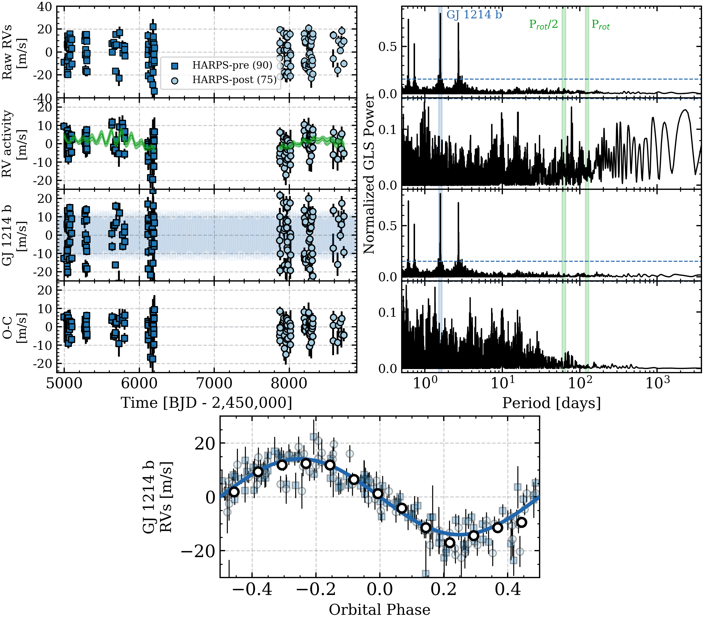
Figure 2: The pre (circles) and post (squares) fiber-upgrade HARPS RVs of GJ 1214. In descending order, the left column depicts the RV time series of the raw RVs, the RV activity component, the GJ 1214 b planetary component, and the RV residuals. The resulting residual rms values for the pre and post fiber-upgrade RVs are 6.2 and 4.7 m s^-1, respectively. The right column depicts the corresponding GLS periodogram. The vertical bands highlight the orbital period of GJ 1214 b ($P=1.58$ days), the stellar rotation period ($P_{\rm rot}$ $=124.7$ days) and its first harmonic ($P_{\rm rot}/2=62.4$ days). The dashed horizontal lines in each periodogram panel depict the 1% FAP. Bottom panel: the activity-corrected RVs phase-folded to the orbital solution of GJ 1214 b.

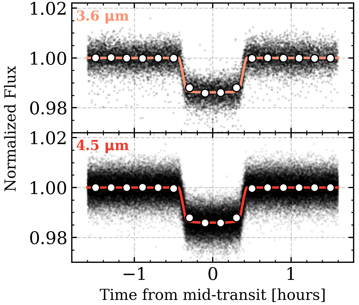
Figure 3: Phase-folded Spitzer/IRAC transit light curves of GJ 1214 b. Upper panel: three 3.6 µm transits. Lower panel: fourteen 4.5 µm transits. Solid curves depict the MAP transit model in each IRAC channel. White circle markers depict the photometry binned for visualization purposes.

We first correct the raw RVs for the deterministic secular acceleration of GJ 1214 (i.e. 0.3 m/s/yr). We then fit the RVs with a Keplarian orbital solution for GJ 1214 b plus an RV activity model trained on the STELLA photometry (Section 4.1). In addition to the shared transit model parameters $\{P,T_{0},h,k\}$, the Keplerian solution includes the RV semiamplitude $K$, which we sample logarithmically in our MCMC. Our RV model also features velocity offset $\gamma$ and logarithmic scalar jitter $\ln{s_{\rm RV}}$ parameters for the subsets of our HARPS RV time series corresponding to the pre and post fiber-upgrade. Similarly to the GP training step, our RV activity model is described by the hyperparameters $\{\ln{a_{\rm RV}},\ln{\lambda_{\rm GP}},\ln{\Gamma_{\rm GP}},\ln{P_{\rm rot}}\}$, with the latter three being shared with our training model on the STELLA photometry. Our full transit plus RV model consists of 24 parameters: $\{M_{s},R_{s},P,T_{0},b,h,k,(r_{p}/R_{s})_{3.6},u_{1,3.6},u_{2,3.6},F_{0,3.6},$ $(r_{p}/R_{s})_{4.5},u_{1,4.5},u_{2,4.5},F_{0,4.5},\ln{K},\gamma_{\rm pre},\gamma_{\rm post},\ln{s_{\rm pre}},$ $\ln{s_{\rm post}},\ln{a_{\rm RV}},\ln{\lambda_{\rm GP}},\ln{\Gamma_{\rm GP}},\ln{P_{\rm rot}}\}$. Our adopted priors are outlined in Table 6.

Similarly to the training step, we sample the posterior of our transit plus RV model parameters using the emcee MCMC code and use the celerite package to construct the GP. We use the resulting maximum a-posteriori (MAP) GP hyperparameters to construct the predictive GP distributions for the pre and post fiber-upgrade time series. We adopt the mean functions of each GP posterior as our best-fit activity models, which are highlighted in the second row of Figure 2. The MAP values of the remaining parameters are reported in Table 6. We use these parameters to compute the Keplerian orbital solution shown in Figure 2 and the 3.6 and 4.5 µm transit models shown in Figure 3.

4.3 Resulting Physical Planetary Parameters

From our measured planetary parameters we refine the orbital and physical parameters of GJ 1214 b. Similarly to Gillon et al. (2014), our Spitzer/IRAC analysis reveals $r_{p}/R_{s}$ values in the 3.6 and 4.5 µm channels that are consistent within $1\sigma$. We therefore average their marginalized posteriors and measure a planetary radius of $r_{p}=$ $2.742^{+0.050}_{-0.053}$ $R_{\oplus}$. Our analysis of 165 HARPS RV measurements provides the most detailed view of the mass of GJ 1214 b to date. We measure a 27$\sigma$ RV semiamplitude of $14.36\pm 0.53$ m s^-1, which corresponds to a $19\sigma$ planetary mass measurement of $m_{p}=$ $8.17\pm 0.43$ $M_{\oplus}$. We note that with our RV dataset, GJ 1214 b’s mass measurement precision is now limited by the uncertainty in the stellar mass with only a small contribution from the RV semi-amplitude uncertainty. The same remains true for the planet’s radius whose measurement uncertainty is dominated by the uncertainty in the stellar radius Gillon et al. (2014). Taking $r_{p}$ and $m_{p}$ together, we recover a $13\sigma$ detection of the planet’s bulk density: $2.20^{+0.17}_{-0.16}$ g cm^-3.

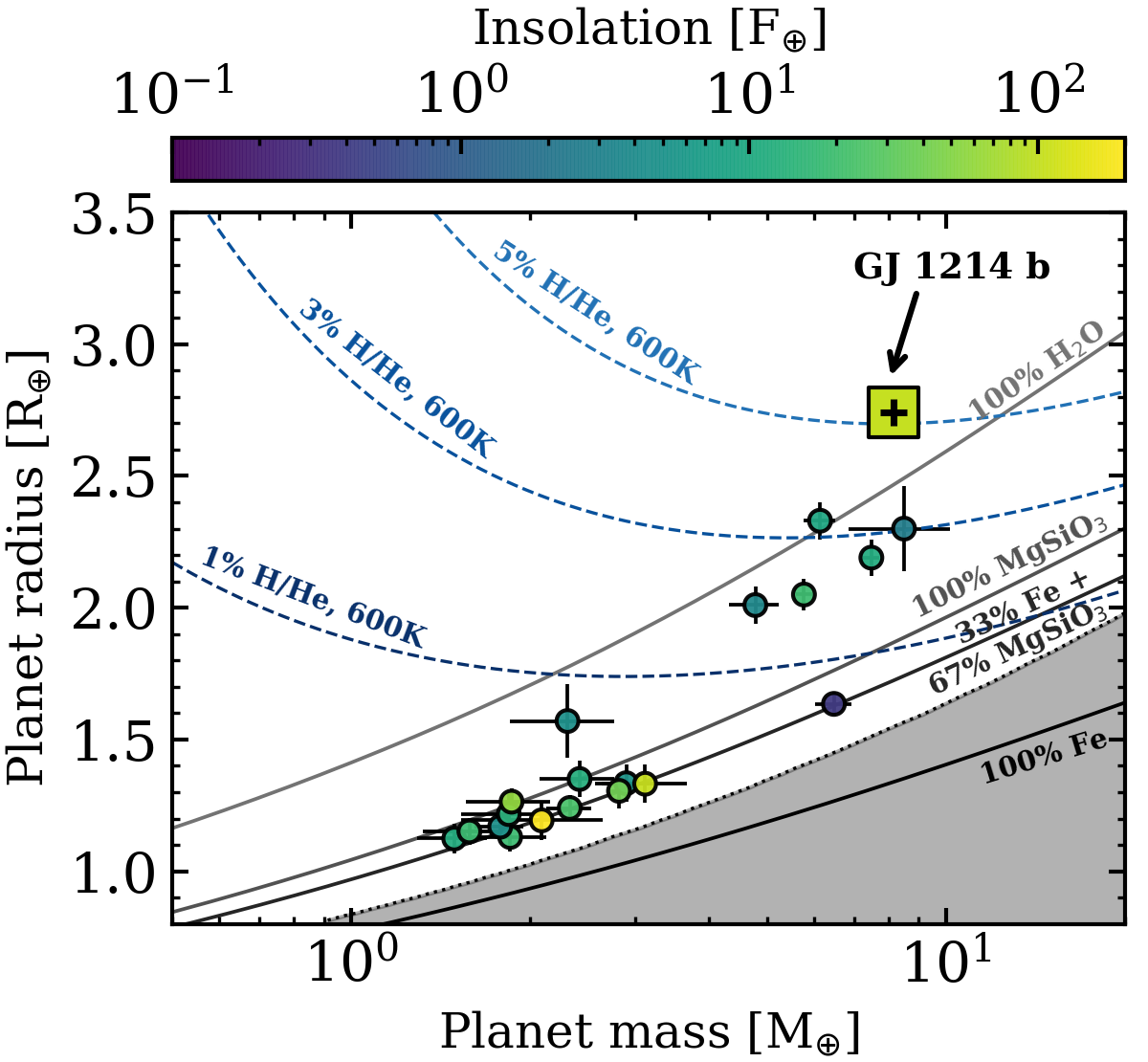
Figure 4: Mass–radius-insolation diagram for small planets with masses measured to $\leq 33$% and orbiting mid-M dwarfs ($M_{s}\in[0.1,0.4]$ $M_{\odot}$). GJ 1214 b is depicted by the large square marker. The solid curves depict internal structure models with mass fractions of 100% water, 100% silicate rock, 33% iron plus 67% rock (i.e. Earth-like), and 100% iron (Zeng & Sasselov, 2013). The dashed curves depict models of Earth-like cores enshrouded in solar metallicity H/He envelopes at the zero-albedo equilibrium temperature of GJ 1214 b (i.e. 600 K) and with various envelope mass fractions. The shaded region bounded by the dotted curve highlights the forbidden region according to models of maximum collisional mantle stripping by giant impacts (Marcus et al., 2010).

We include the refined mass and radius of GJ 1214 b in the mass-radius diagram of small planets orbiting mid-M dwarfs in Figure 4. When compared to two-layered, solid structure models (Zeng & Sasselov, 2013), we see that GJ 1214 b’s low bulk density is clearly inconsistent with a purely solid body and therefore requires an extended H/He envelope to explain its mass and radius. With the inclusion of a gaseous envelope component, we are unable to place meaningful constraints on the mass fraction of materials that compose the planet’s underlying structure. However, population synthesis models of small close-in planets indicate that planets that form the sub-Neptune peak in the M dwarf radius valley (Hirano et al., 2018; Cloutier & Menou, 2020) are likely enveloped terrestrials rather than volatile-rich planets (Owen & Wu, 2017; Gupta & Schlichting, 2019; Rogers & Owen, 2021). If we assume that GJ 1214 b is in fact an enveloped terrestrial, we can calculate the envelope mass fraction $X_{\rm env}\equiv m_{\rm env}/m_{p}$ required to explain its mass and radius. We perform this calculation assuming that GJ 1214 b consists of an Earth-like core with a 33% iron core mass fraction and hosts a H/He envelope with solar-metallicity ($\mu=2.35$). The thermal structure of the gaseous envelope is described by the semi-analytical radiative-convective model from (Owen & Wu, 2017). We sample GJ 1214 b’s joint $\{m_{p},r_{p},T_{\rm eq}\}$ posterior and calculate the core and envelope masses required to match the mass and radius of GJ 1214 b with an isothermal upper atmosphere at $T_{\text{eq}}$. We measure an envelope mass fraction of $X_{\rm env}=$ $5.24^{+0.30}_{-0.29}$%. We note that the uncertainty on $X_{\rm env}$ reported here is determined solely by the uncertainties in the input parameters $\{m_{p},r_{p},T_{\rm eq}\}$ and does not include uncertainties in the physical model.

4.4 Orbital Eccentricity Result

Our joint transit plus RV analysis, together with a-priori constraints on the stellar density, produces a strong constraint on GJ 1214 b’s orbital eccentricity. The marginalized posterior on the orbital eccentricity heavily favors a circular orbital solution. We find that $e<$ $0.063$ and $<$ $0.100$ at 95% and 99% confidence, respectively. Although a circular orbit is expected given the planet’s short circularization timescale of $<1$ Myr, precise knowledge of the quantity $e\cos{\omega}$ has critical consequences for scheduling secondary eclipse observations with facilities such as JWST. The value of $e\cos{\omega}$ directly translates into an uncertainty window on the eclipse center time according to

$$\Delta t=\frac{2}{\pi}\,P\,e\cos{\omega}.$$ (4)

Our stringent constraints on $e\cos{\omega}$ translate into an uncertainty on the center time of eclipse of 2.8 hours at 95% confidence, or approximately 3.2 times the eclipse duration of 53 minutes.

5 Limits on Additional Planets

Continuous photometric monitoring of GJ 1214 with Spitzer revealed no new transiting planets larger than Mars and interior to the inner HZ at 20.9 days (Gillon et al., 2014). Furthermore, TTV searches have not yielded any additional planetary signals (Carter et al., 2011; Harpsøe et al., 2013; Fraine et al., 2013; Gillon et al., 2014). With our intensive RV time series we are able to place meaningful constraints on additional planets orbiting GJ 1214, which need not be in a transiting configuration, nor locked into a mean-motion resonance with GJ 1214 b where the TTV sensitivity is maximized. Here we derive limits on the existence of additional planets around GJ 1214 via a set of injection-recovery tests into our RV time series.

5.1 Injection-Recovery Methodology

We conduct a pair of Monte Carlo (MC) simulations to calculate the detection sensitivity of planets as a function of planet mass and orbital period. The MC simulations differ in their noisy RV time series into which we will inject planetary signals.

MCI: we sample the Gaussian distribution $\mathcal{N}(0,\sigma_{\rm eff})$ at the times of our HARPS pre and post-fiber upgrade window functions. The effective RV noise $\sigma_{\rm eff}$ values are calculated from the quadrature addition of the median RV uncertainties and the MAP scalar jitters from our RV analysis ($\sigma_{\text{eff,pre}}=4.53$ m s^-1, $\sigma_{\text{eff,post}}=3.99$ m s^-1). However in practice, RV uncertainties are never purely Gaussian, often as a result of variable observing conditions or imperfect corrections of instrumental drifts. To mimic these stochastic effects, we add a unique noise term to the RV dispersion by sampling from $\mathcal{U}(-1,1)$ m s^-1, whose limits are generally appropriate for HARPS observations. The MCI simulations should be interpreted as a best case scenario in that the noisy RVs are uncontaminated by temporally-correlated signals from stellar activity, which are implicitly assumed to have been perfectly mitigated.

MCII: alternatively, we construct noisy RVs by subtracting the MAP Keplerian signal of GJ 1214 b from the pre and post fiber-upgrade RVs (see second row in Figure 2). In this way, signals from the window function and stellar activity are preserved. The MCII simulations can be interpreted as a worst case scenario wherein stellar activity is left uncorrected and will contribute to the rms of the RVs. This effect will be particularly detrimental to the recovery of injected planetary signals close to $P_{\rm rot}$ (Newton et al., 2016; Vanderburg et al., 2016). However undesirable the persistence of stellar activity, and aliases, are for planet searches, these effects make the MCII results a more realistic assessment of the detection sensitivity compared to MCI.

In each of the $10^{5}$ MC realizations in MCI and MCII, we inject a single synthetic Keplerian signal into the noisy HARPS RVs. We note that searching for individual planets in our injection-recovery tests is a simplification as blind searches for multiple RV planets are often conducted simultaneousy rather than iteratively, such that the detection sensitivity is not independent of the number of planetary signals. The masses and periods of our synthetic planet population are sampled uniformly in log-space between 0.1-20 $M_{\oplus}$ and 0.5-200 days, respectively. We select these outer bounds with the intention to cover the majority of the parameter space which is spanned by known planets around mid-M dwarfs (see Section 6). Our adopted mass range encapsulates planets with masses smaller than that of Neptune (i.e. 17 $M_{\oplus}$). The mass of GJ 1214 is sampled from its posterior $\mathcal{N}(0.178,0.010)$ $M_{\odot}$. Due to the transiting nature of GJ 1214 b and the characteristically low dispersion in mutual inclinations among Kepler multi-planet systems with $a/R_{s}>5$ (Dai et al., 2018), we focus on orbital inclinations that are nearly co-planar with GJ 1214 b ($i_{b}=88.7\pm 0.1^{\circ}$) by sampling inclinations from $\mathcal{N}(i_{b},\sigma_{i})$, where $\sigma_{i}=2^{\circ}$ (Ballard & Johnson, 2016; Dai et al., 2018). Planets’ orbital phases are sampled from $\mathcal{U}(-\pi,\pi)$ and all orbits are assumed to be circular.

We inject the synthetic planetary signal in each realization and attempt to recover the injected signal based on two criteria in MCI plus one additional criterion in MCII. Because the search for non-transiting planets lacks the luxury of a-priori knowledge of the planet’s ephemeris, a non-transiting planet’s signal in an RV time series must emerge as a prominent periodicity in the data. As such, our first criterion for the successful recovery of an injected planet is that the maximum GLS periodogram power within 10% of the injected period must exceed a FAP of 1%. However, sporadic peaks in the GLS periodogram can masquerade as a planetary signal. We safeguard against these false positives by insisting that a six-parameter Keplerian model at the GLS peak’s orbital period must be strongly favored over the null hypothesis (i.e. a flat line with a velocity offset). For this model comparison, we calculate the Bayesian Information Criteria (BIC) for the Keplerian model and for the null model. The BIC $=-2\ln{\mathcal{L}}+\nu\ln{N}$, where $\mathcal{L}$ is the likelihood of the RV data given the model, $\nu$ is the number of model parameters ($\nu=6$ or 1 for the Keplerian and null models, respectively), and $N=165$ is the number of RV measurements. Taken together, we claim the successful recovery of an injected planet in MCI if 1) the GLS power of the injected periodic signal has FAP $<1$%, and 2) the BIC of the null hypothesis is greater than ten times the BIC of the Keplerian model.

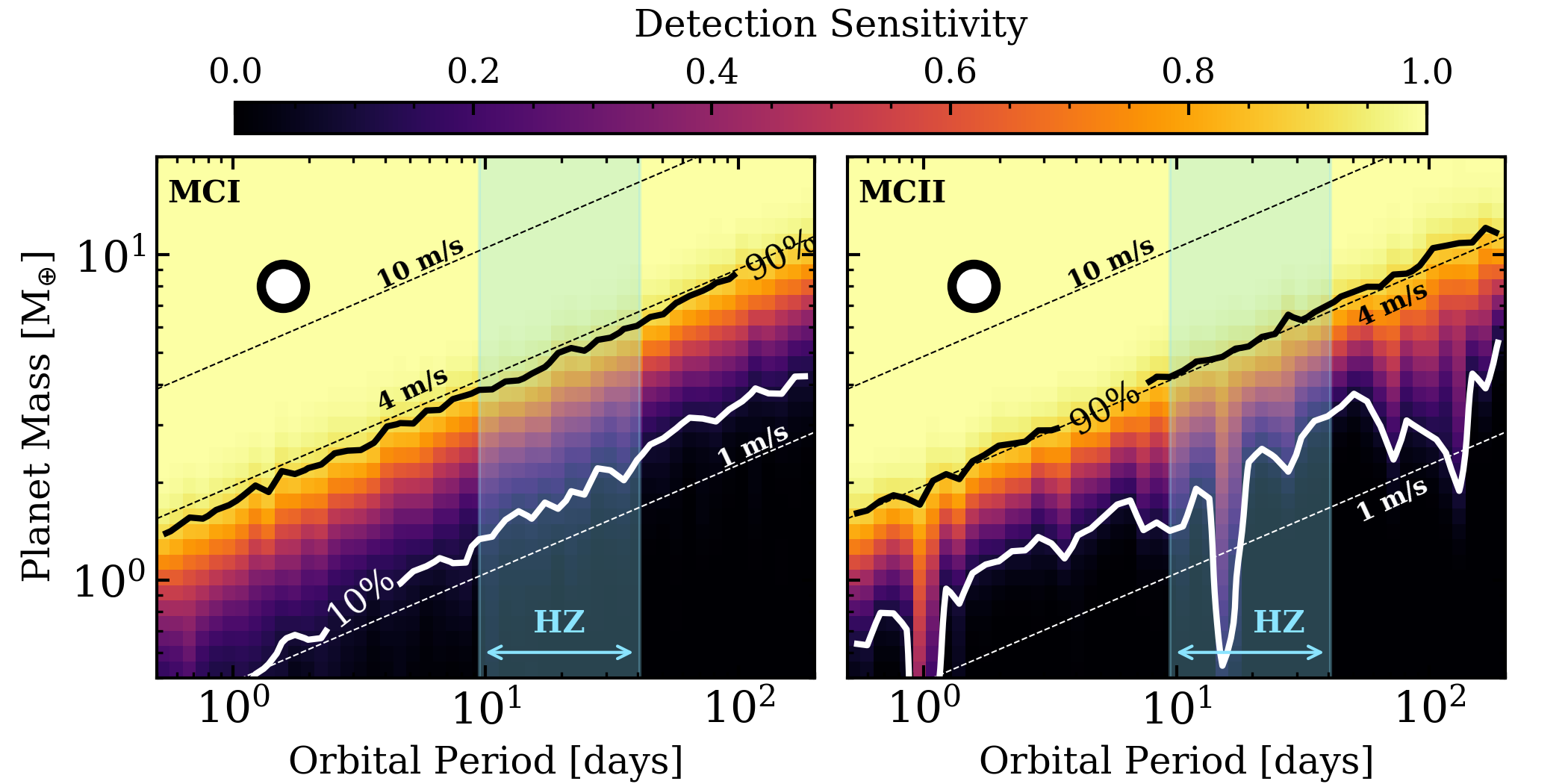
Figure 5: RV detection sensitivity to planets orbiting GJ 1214 as a function of planet mass and orbital period for two noise models. Left panel: the results of the MCI simulation, which should be interpreted as a best case scenario. Right panel: the results of the MCII simulation, which should be interpreted as the worst case scenario (see Section 5.1 for details). The solid contours highlight the 10% and 90% sensitivity levels. The thin dashed lines represent lines of constant semiamplitude with illustrative values equal to 1, 4, and 10 m s^-1. The circle markers highlight GJ 1214 b. The vertical shaded regions span the habitable zone of GJ 1214.

The noisy RVs in MCI do not contain any temporally correlated signals such that there are no significant peaks in the GLS periodogram of the noisy RVs. However, the MCII noisy RVs retain the stellar activity signals which can produce GLS periodogram peaks at $P_{\rm rot}$, one of its low order harmonics, or at spurious periods unrelated to stellar rotation (Nava et al., 2020). We therefore apply a third condition to the successful recovery of an injected Keplerian signal in MCII. Namely, the largest peak in the GLS periodogram of the noisy RVs within 10% of the injected period must have FAP $>1$%. This is to ensure that the injected signal is not confused with a residual signal or an alias close to the its orbital frequency. Alternatively, if the BIC of the null hypothesis is greater than $10^{3}$ times the BIC of the Keplerian model, then we continue to accept the injected signal as a detection because such RV signals have very high S/N and should not be rejected by relatively minor aliases present in the window function.

Due to the exhaustive nature of computing the GLS periodogram and its corresponding FAP in $2\times 10^{5}$ realizations via bootstrapping with replacement, we adopt an analytical framework to approximate the FAP as a function of the normalized GLS power $p$ (Cumming, 2004). For a time series containing $N$ measurements and spanning $T$ days, the FAP is well-approximated by

$$\text{FAP}(p_{0})=1-[1-\text{Pr}(p>p_{0})]^{M},$$ (5)

where $M=\Delta f/\delta f$ is the number of sampled independent frequencies and is calculated from the ratio of the frequency range $\Delta f=f_{2}-f_{1}$ and the frequency resolution $\delta f=1/T$. For a GLS periodogram normalized by the sample variance, such that the GLS power is bounded between 0 and 1 (Zechmeister & Kürster, 2009), the probability term in Eq. 5 becomes $\text{Pr}(p>p_{0})=(1-p_{0})^{(N-3)/2}$ (Cumming et al., 1999), where $p_{0}$ is the power whose FAP we are interested in. Adopting this analytical formalism significantly decreases the computation time of the MC simulations and enables the mass-period space to be sampled more efficiently.

5.2 RV Detection Sensitivity

We calculate the RV detection sensitivity in each MC simulation as the ratio of the number of recovered planets to the number of injected planets as a function of mass and period. Our results are shown in Figure 5.

The results from MCI indicate that the sensitivity is a smooth function of RV semiamplitude. Injected planetary signals with $K\gtrsim 4$ m s^-1 are detected $>90$% of the time. The sensitivity contours derived from MCII are broadly similar with the 90% contour being well-aligned with $K=4$ m s^-1 as in MCI. However in MCII, residual low FAP frequencies in the HARPS RVs after the removal of GJ 1214 b disrupt the smoothness of the map. In particular, residual GLS peaks introduce structure in the sensitivity map, which can in principle inhibit the detection of planetary signals whose orbital periods are close to low FAP peaks (or aliases thereof) in the window function. However, the persistent periodicities seen in the GJ 1214 RV residuals at 1, 16, and 125 days have FAPs $>1$% such that they are not confused with injected signals with similar orbital periods. But because these periodicities do exhibit a slightly enhanced GLS power, the GLS power of injected planets near these frequencies is artificialy enhanced. This effect manifests itself as a moderate improvement to the sensitivity in the second panel of Figure 5. We caution that these enhancements are an undesirable outcome of a periodogram-based recovery process and should not be taken at face value in a planet search.

The residual signals at 1 and 125 can be easily explained by the daily alias and the rotation period of GJ 1214, respectively. However, the signal at approximately 16 days is not trivially explained by a stellar rotation harmonic or by an alias from the HARPS window function. The FAP of the 16-day signal in the MCII RV residuals (i.e. without removing a GP) exceeds 1% such that the evidence for a periodic signal at 16 days is marginal. Furthermore, the GLS periodogram of the RV residuals following the removal of GJ 1214 b and the GP activity model does not show any significant power at 16 days (see the fourth row in Figure 2). As a check, we conducted a separate RV analysis that included a second Keplerian signal with a narrow uniform prior on its orbital period centered on 16 days. The resulting marginalized posterior on the Keplerian semiamplitude is consistent with zero and has an upper limit of 2.45 m s^-1 at 95% confidence (i.e. corresponding to $m_{p}\sin{i}$ $<3.03$ $M_{\oplus}$). Together these tests indicate that there is no strong evidence for a second planet near 16 days but continued RV follow-up will help to establish the nature of this signal.

Modulo the detailed structure in the MCII detection sensitivity, the results are broadly consistent with MCI. The similarity between each MC simulation’s detection sensitivity is depicted in Figure 6 as a function of $K$. The two MC simulation curves are in close agreement for all values of $K$ with the MCII sensitivity exhibiting a slight detriment relative to MCI up to $K\geq 5$ m s^-1, at which point all planetary signals within 200 days are detectable. Focusing on the more realistic results from MCII and taking the 90% contour to mark the boundary between detection and non-detection, we are able to rule out additional planets around GJ 1214 above 4 $M_{\oplus}$ and within 10 days. By adopting the empirical recent Venus and early Mars limits of the inner and outer habitable zone (HZ) from Kopparapu et al. (2013), we can rule out planets down to 5 $M_{\oplus}$ within the HZ. The most massive Super-Earths have masses $\lesssim 7$ $M_{\oplus}$ (LHS 1140 b; Ment et al. 2019, TOI-1235 b; Cloutier et al. 2020b), such that we are only able to rule out the most massive HZ rocky planets.

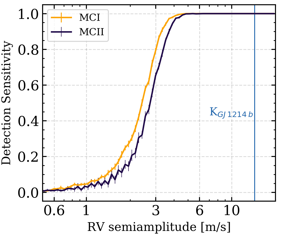
Figure 6: RV detection sensitivity to planets orbiting GJ 1214 as a function of RV semiamplitude for two noise models. The gold and blue curves depict the RV detection sensitivity from the MCI and MCII simulations, respectively. The errorbars illustrate the error on the mean detection sensitivity in each semiamplitude bin. The vertical solid line highlights the semiamplitude of GJ 1214 b.

Within our sensitivity limits, GJ 1214 continues to be a system with only one known planet. In the next section, we will argue that this result is somewhat surprising. We will show that multi-planet systems around mid-M dwarfs are common and that GJ 1214 belongs to a small subset of mid-M dwarf systems that appear to be singles given the current RV data available.

6 The Frequency of Multi-Planet Systems Around Mid-M Dwarfs

The Kepler transit survey revealed that multi-planet systems around early M dwarfs are ubiquitous (e.g. Dressing & Charbonneau, 2015; Ballard & Johnson, 2016; Gaidos et al., 2016; Hsu et al., 2020). Studies focused on later type M dwarfs have shown preliminary evidence of a trend of increasing small planet multiplicity with decreasing stellar mass. Although the current inferences are largely limited by poor counting statistics around mid-to-late M dwarfs (Muirhead et al., 2015; Hardegree-Ullman et al., 2019). If it is true that mid-M dwarf planetary systems frequently host multiple planets, then the confirmation of even a single transiting planet around a mid-M dwarf would establish a strong prior on the existence of additional planets. Indeed, a number of apparently single transiting mid-M dwarf systems have revealed additional planets in RV follow-up campaigns (GJ 357c,d; Luque et al. 2019, GJ 1132c; Bonfils et al. 2018b, GJ 3473c; Kemmer et al. 2020, LHS 1140c; Ment et al. 2019). Here we aim to quantify this phenomenon by calculating the frequency of mid-M dwarf planetary systems that host multiple planets.

6.1 Calculating the Frequency of Mid-M Dwarf Planetary Systems with Multiple Planets

Let $f$ denote the fraction of mid-M dwarf planetary systems that host two or more planets over some range of planet masses and orbital periods. That is, among the sample of mid-M dwarfs that host at least one known planet, $f$ denotes the fraction of those planetary systems that host multiple planets. To calculate $f$, we will consider $N$ mid-M dwarfs that host at least one known planet (see Section 6.1.1), which we index by $i=1,\dots,N$. For each mid-M dwarf in our sample, we define $p_{i}\equiv$ the RV detection sensitivity to additional planets over the range of planet masses $\in[m_{p,\rm min},m_{p,\rm max}]$ and orbital periods $\in[P_{\rm min},P_{\rm max}]$. We will compute the $p_{i}$ values in Section 6.1.2. Because each planetary system contains at least one confirmed planet, the probability of detecting an additional planet proceeds as a Bernoulli process with probability $fp_{i}$. We denote the results of the $N$ Bernoulli experiments by the set of binary values $\{k_{i}\}$ wherein $k_{i}=1$ if the $i^{\rm th}$ system contains multiple planets, with at least one planet having $m_{p}\in[m_{p,\rm min},m_{p,\rm max}]$ and $P\in[P_{\rm min},P_{\rm max}]$. Otherwise, $k_{i}=0$. For example, in Section 5.2 we showed that GJ 1214 appears to be a single-planet system such that $k_{\rm GJ1214}=0$, whereas for the two-planet system LHS 1140, $k_{\rm LHS1140}=1$. The likelihood of measuring $\{k_{i}\}$ from $N$ systems is given by

$$\mathcal{L}(\{k_{i}\}|f,\{p_{i}\})=\prod_{i=1}^{N}\>(fp_{i})^{k_{i}}\>(1-fp_{i})^{1-k_{i}}.$$ (6)

Assuming that all values of $f$ are equally probable (i.e. $\text{Pr}(f)=1$), the normalized posterior of $f$ follows from Bayes theorem:

$$\text{Pr}(f|\{k_{i}\},\{p_{i}\})=\frac{\mathcal{L}(\{k_{i}\}|f,\{p_{i}\})}{\int_{0}^{1}\mathcal{L}(\{k_{i}\}|f,\{p_{i}\})df},$$ (7)

which we can use to calculate $f$ and its corresponding confidence intervals.

6.1.1 Sample of Mid-M Dwarf Systems

We proceed with measuring $f$ by compiling the set of mid-M dwarfs with

1. $M_{s}\in[0.1,0.4]$ $M_{\odot}$, and

2. that host at least one confirmed planet with an RV mass measurement.

Because our second condition requires systems to contain at least one confirmed planet with an RV mass measurement, we only consider transiting planetary systems because the absolute masses of non-transiting planets uncovered in RV datasets are unmeasurable. The existence of a mass detection also (largely) implies that sufficient RV follow-up was conducted and a robust RV detection sensitivity has been achieved. This will enable meaningful constraints on $f$ to be produced. We note that our second criterion excludes systems with TTV masses only. This is desirable given the difficulty in accessing the TTV sensitivity to additional planets; a function which itself is not smooth with orbital separation due to the dependence of the TTV amplitude on the proximity of planet pairs to low-order mean motion resonances. We identify $12$ transiting planetary systems based on our criteria and list them in Table 4.

Table 4: Summary of known mid-M dwarf transiting planetary systems with RV follow-up

Star name	$M_{s}$	Number	Average RV	Ref.
	[$M_{\odot}$]	of known	Sensitivity,
		planets	$p_{i}$ [%]
GJ 1214	$0.178$	1	65.8	this work
LHS 1140	$0.179$	$\geq 2$	75.7	Me19,Li20
GJ 1132	$0.191$	2	73.4	Bo18b
LHS 1478	$0.235$	1	52.5	So21
LTT 1445A	$0.257$	2	66.2	Wi21 submitted
L 98-59	$0.313$	3	57.0	Cl19
GJ 486	$0.323$	1	94.8	Tr21
GJ 3473	$0.371$	2	43.3	Ke20
GJ 357	$0.380$	2	54.7	Lu19
GJ 1252	$0.381$	1	14.1	Sh20
LTT 3780	$0.399$	2	60.0	Cl20,No20
TOI-270	$0.400$	3	65.2	Va21

One notable system is excluded from our sample on the basis of having TTV masses only without substantial RV follow-up (K2-146; Hamann et al., 2019). Other notable exclusions include the nearby system LHS 3844 (Vanderspek et al., 2019) and the multi-transiting system around LP 791-18 (Crossfield et al., 2019), both of which lack published RV time series.

6.1.2 RV Detection Sensitivity

We compute each system’s RV detection sensitivity $p_{i}$ identically to the procedure described in Section 5.1 as applied to our GJ 1214 RV data (i.e. via injection-recovery tests in the RV time series). We retrieve each system’s RV time series from its literature source listed in Table 4. For the MCI simulations, we construct the noisy RVs from the quadrature addition of the median RV uncertainty and the scalar jitter for each unique spectrograph. In the MCII simulations, we subtract the orbtial signal for each known planet using the Keplerian parameters reported in the reference. The planet injections and subsequent recoveries proceed identically as with GJ 1214. The resulting sensitivity maps for each mid-M dwarf are displayed in Appendix B.

6.1.3 The Frequency of Multi-Planet Systems Around Mid-M Dwarfs

After tabulating $\{k_{i}\}$ and calculating $\{p_{i}\}$ among the mid-M dwarfs in our sample, we compute the posterior of $f$ using Eq. 7. Due to the relatively small number of mid-M dwarf systems with at least one known transiting planet, we consider a wide range of planetary parameters bounded by $m_{p}\in[1,10]$ $M_{\oplus}$ and $P\in[0.5,50]$ days. However, because the typical RV detection sensitivity varies widely across such a wide range of parameters (c.f. Figure 5), our results as discussed below only apply under the assumption that planets are distributed uniformly as a function of $\log{m_{p}}$ and $\log{P}$, both of which are implicitly assumed based on our sampling of injected planets. Of the $12$ systems in our sample, eight host a multi-planet system with at least one planet within the aforementioned mass and period bounds. The resulting $f$ posteriors from MCI and MCII are depicted in Figure 7. The MAP values of $f$, along with confidence intervals bounded by the 16^th and 84^th percentiles are $86^{+6}_{-20}$% and $90^{+5}_{-21}$% for MCI and MCII, respectively. The 95% lower limits on $f$ are $>57$% and $>59$% for MCI and MCII, respectively. The consistency of $f$ between both MC simulations highlights the insensitivity of our results to the exact method of constructing the noisy RVs.

The consensus from our calculations is that the most likely fraction of mid-M dwarf planetary systems that host multiple planets less massive than 10 $M_{\oplus}$ and within 50 days is approximately 90%. To rephrase, the discovery of a single planet within these bounds around a mid-M dwarf establishes a strong prior that favors the existence of at least one additional planet in the system.

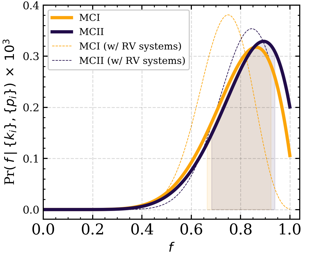
Figure 7: The posterior probability of $f$: the fraction of mid-M dwarf planetary systems that host multiple planets with masses $m_{p}\in[1,10]$ $M_{\oplus}$ and orbital periods $P\in[0.5,50]$ days. The analytical $f$ posterior is calculated using Eq. 7 given the mid-M dwarfs with multiple planets $\{k_{i}\}$ and their respective RV detection sensitivities $\{p_{i}\}$. The solid gold curve depicts the result using the detection sensitivities from MCI whereas the solid blue curve depicts the result from MCII (see Section 5.1). As a check, the dashed curves depict the $f$ posterior from each MC when RV planetary systems are included in the calculation (see Section 6.1.4).

6.1.4 Including RV Systems When Calculating $f$

Our previous calculation of $f$ focused solely on transiting planets whose absolute masses are measured with an RV detection. Here we relax this requirement by equating minimum planet mass $m_{p}\sin{i}$ to planet mass, which allows us to include $15$ additional mid-M dwarf planetary systems (Table 5). We construct our RV planet sample by retrieving planets with $m_{p}\sin{i}$ $\in[1,10]$ $M_{\oplus}$, $P\in[0.5,50]$ days, and whose dispositions have not been directly contested in the literature. Our sample of RV planets is compared to the transiting planet sample in $P$-$m_{p}$ space in Figure 8. Most of the RV planets have minimum masses and periods that are distinct from the transiting planet sample. RV planets often have longer orbital periods because of the geometric selection effect of decreasing transit probability with increasing orbital period. Many of the RV planets are also less massive than the transiting planets because their host stars tend to be brighter, which often results in more intensive RV follow-up and with higher S/N measurements, both of which facilitate the detection of low amplitude signals.

Table 5: Summary of known mid-M dwarf RV planetary systems

Star name	$M_{s}$	Number	Average RV	Ref.
	[$M_{\odot}$]	of known	Sensitivity,
		planets	$p_{i}$ [%]
Prox Cen	$0.122$	$\geq 1$	47.0	An16,Su20
GJ 1061	$0.123$	3	74.3	Dr20
YZ Ceti	$0.133$	3	86.1	As17a
GJ 3323	$0.166$	2	76.2	As17b
GJ 1265	$0.168$	1	59.0	Lu18
Ross 128	$0.173$	1	81.7	Bo18a
GJ 3779	$0.264$	1	50.4	Lu18
Wolf 1061	$0.302$	3	71.5	As17b
GJ 581	$0.311$	3	72.5	Tr18
GJ 273	$0.314$	2	22.0	As17b
GJ 625	$0.320$	1	69.7	Su17
GJ 667C	$0.330$	$\geq 2$	57.1	An13
GJ 876	$0.350$	4	72.0	Tr18
GJ 251	$0.360$	1	64.3	St20
GJ 411	$0.386$	1	71.2	Dí19

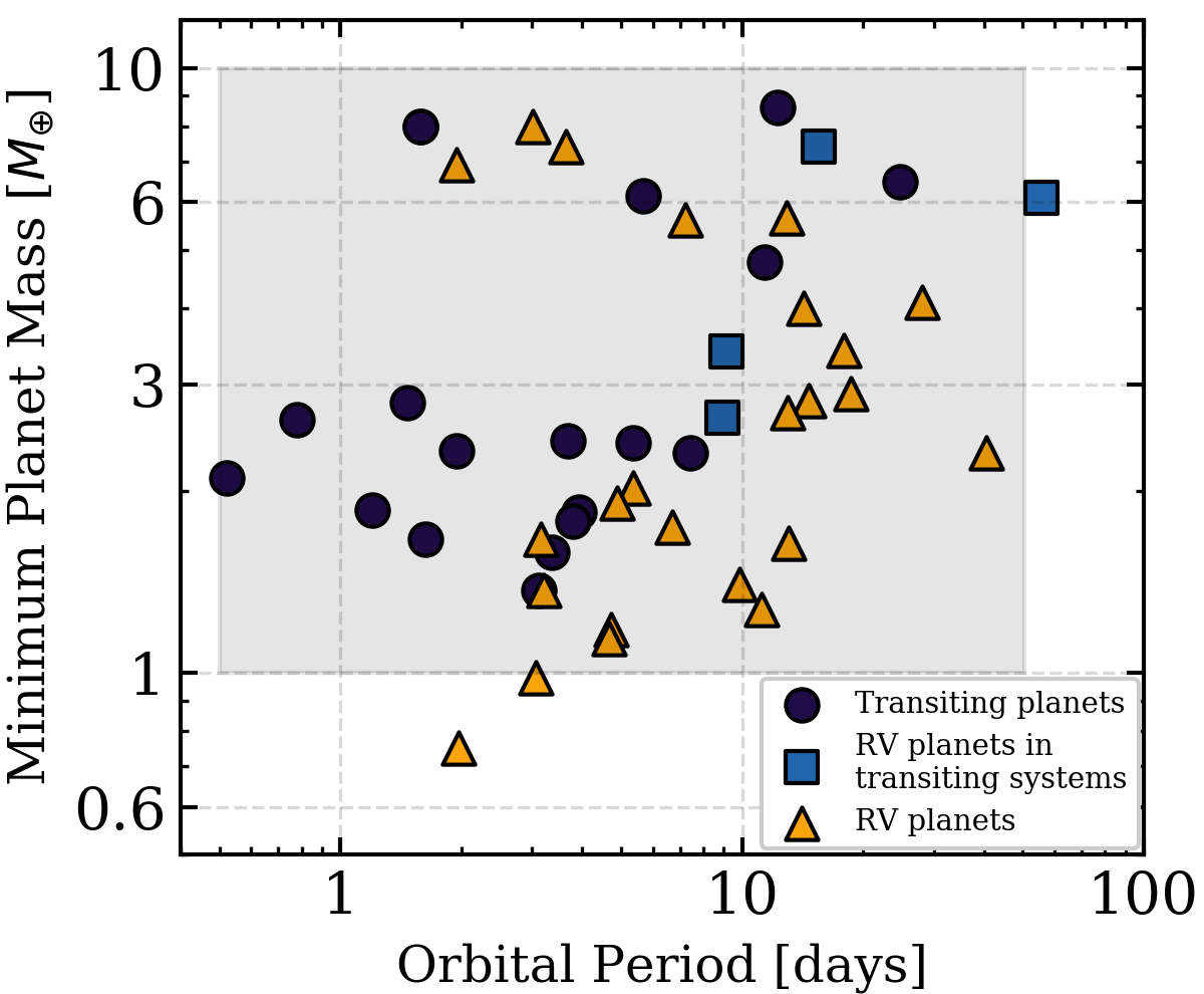
Figure 8: Minimum masses and orbital periods of planets orbiting mid-M dwarfs and with an RV mass detection. The circles depict 19 transiting planets in $12$ systems. The squares depict four RV planets in three transiting planetary systems. The triangles depict the 31 RV planets in $15$ systems. The shaded rectangle outlines the range of planetary parameters over which we calculate $f$ in this work.

We wish to include the set of confirmed RV planets into our calculation of $f$. We proceed by computing each system’s detection sensitivity $\{p_{i}\}$ via injection-recovery in a manner similar to the transiting planetary systems. The only difference being that we modify the distribution from which the injected planet’s inclinations are drawn. Because the orbital inclinations $i$ of RV planets are unconstrained, we draw $i$ from the distribution that is uniform in $\cos{i}$: i.e. $i$ drawn from $\arccos{\mathcal{U}(-1,1)}$. In general, this geometric effect is detrimental to the RV detection sensitivity because it allows for the possibility of nearly face-on orbits for which the RV semiamplitude goes to zero given its linear dependence on $\sin{i}$. The resulting sensitivity maps for each mid-M dwarf in our RV sample are included in Appendix B.

By combining the $15$ RV systems with the $12$ transiting systems, we expand the sets $\{k_{i}\}$ and $\{p_{i}\}$. We note that tentative evidence for additional planet candidates orbiting Proxima Centauri at 5.15 days (Suárez Mascareño et al., 2020) and at 5.2 years (Damasso et al., 2020) have been independently reported. However, due to the present uncertainties regarding the nature of these signals, here we will treat Proxima Centauri as a single-planet system (i.e. $k_{\rm Prox}=0$). We note that the resulting value of $f$ is largely insensitive to any one system and that if instead we set $k_{\rm Prox}=1$, the resulting value of $f$ will only increase by 3%. With $8/15=53$% of RV systems hosting multiple planets over the range of interest, the sample of RV systems exhibits a slightly lower fraction of known multi-planet systems compared to the transiting systems ($8/12=68$%). However despite having fractionally fewer multi-planet systems and systematically larger detection sensitivities, we find that the $f$ values obtained when RV systems are included in the calculation are consistent with those obtained from transiting systems only (Figure 7). Explicitly, including RV planets in MCI we measure $75^{+9}_{-12}$%, compared to $86^{+6}_{-20}$% with transiting systems alone. Similarly in MCII, we measure $85^{+8}_{-15}$%, compared to $90^{+5}_{-21}$% with transiting systems alone. Therefore the following statement continues to be robust: the existence of one known planet orbiting a mid-M dwarf establishes a strong prior that favors the existence of at least one additional planet in the system.

6.2 Is the Architecture of the GJ 1214 System Unique Among Mid-M Dwarfs?

In Section 6.1.3 we calculated that $90^{+5}_{-21}$% of mid-M dwarf planetary systems host multiple planets when at least one planet has $m_{p}\in[1,10]$ $M_{\oplus}$ and $P\in[0.5,50]$ days. Given that GJ 1214 hosts one such planet, and that multi-planet mid-M dwarf systems are extremely common, it may appear contradictory that GJ 1214 does not show evidence for additional planets (Section 5.2). The cause of this apparent discrepancy must be due to either the GJ 1214 system being a bona-fide single-planet system, or that additional planets are present but are undetected due to our imperfect RV sensitivity.

Given GJ 1214’s detection sensitivity over the parameter range of interest (Figure 5), we find the probability that GJ 1214 is a single-planet system to be $44^{+9}_{-5}$. This value is consistent with 50% such that there is no strong evidence that GJ 1214 is a bona-fide single-planet system. For example, if intensive RV characterization were to continue to achieve a detection sensitivity that is on par with that of the mid-M dwarf transiting system with the highest RV sensitivity to-date ($p_{\rm GJ486}=90$%; Trifonov et al., 2021), then we would measure the probability that GJ 1214 is a single-planet system to be $15^{+21}_{-1}$% (if it remained a single-planet system). We estimate that reaching this goal would require an additional 120 hours of observing time with HARPS (Cloutier et al., 2018). But using an alternative spectrograph like MAROON-X, which is optimized for M dwarfs (Seifahrt et al., 2018), the observing time may be signficiantly reduced to about 15 hours. We emphasize however that this calculation is approximate as it does not consider telescope scheduling, overheads, and the unknown effects of effects of stellar activity at red optical wavelengths.

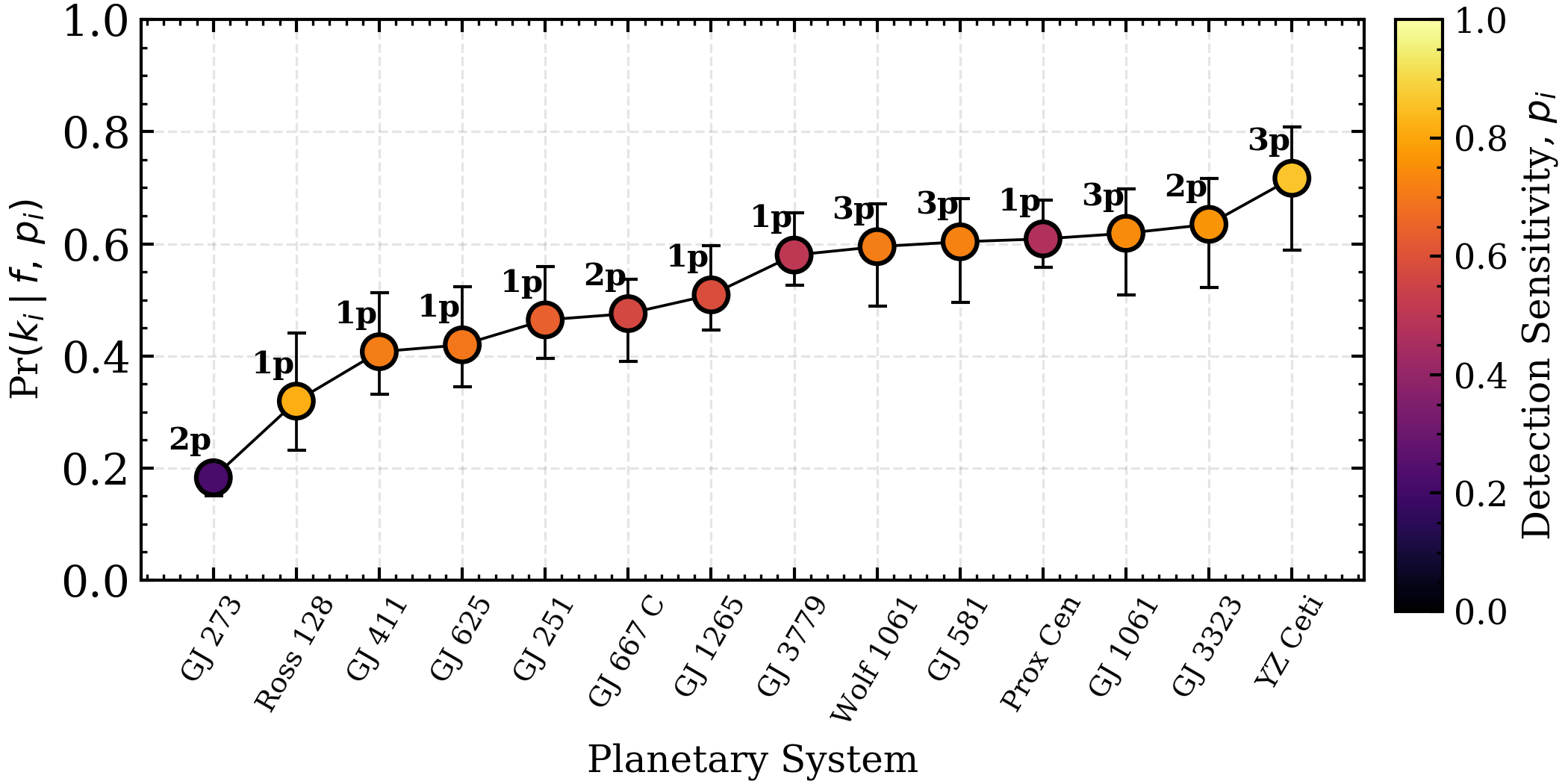
Figure 9: The probability of detecting the either one (i.e. $k_{i}=0$) or multiple planets (i.e. $k_{i}=1$) in each individual mid-M dwarf system with at least one known small planet candidate. Each system’s probability is calculated from the fraction of mid-M dwarf planetary systems with multi-planet systems $f=$ $90^{+5}_{-21}$% and each system’s RV detection sensitivity to planets with $m_{p}\in[1,10]$ $M_{\oplus}$ and $P\in[0.5,50]$ days; $p_{i}$. The uncertainty on $f$ produces the errorbars on each data point. The number of known planet candidates in each system is annotated next to its data point.

6.3 Are All Small RV Planets Detected Around Mid-M Dwarfs Real?

In general, small planets discovered in RV datasets are more difficult to confirm than transiting planets. This is due to the typically lower S/N of RV signals relative to transit signals and the strong impacts that stellar activity and uneven sampling can have on the recovery of RV signals. As a result, small RV planets have a greater probability of being a false positive than their transiting counterparts (e.g. Robertson et al., 2014; Robertson & Mahadevan, 2014; Rajpaul et al., 2016; Lubin et al., 2021).

Using the value of $f$ measured with transiting planets only (i.e. $90^{+5}_{-21}$%), we can calculate the probability that all of the RV planets in our sample are real planets. Among the $15$ RV systems in our sample, $\sum_{i}\,k_{i}=8$ implying that single-planet RV systems may be more common than expected based on the results from the transiting systems where the false positive probability is negligible. Given that the RV detection sensitivities for RV systems are often superior to the transiting planetary systems, we would expect to detect multiple planets in closer to 90% of the RV systems, if those multi-planet systems existed. The fact that only eight out of $15$ (53%) of RV systems appear to be singles presents a discrepancy with the results from the ‘clean’ transiting planet sample. We find that the probability of finding only eight out of $15$ multi-planet mid-M dwarf RV systems to be $<$ $12$% at 99% confidence. That is, mid-M dwarf planetary systems with multiple planets are common and because most of the RV systems with at least one known planet have typically high RV detection sensitivity, it is improbable that such a small fraction of the RV systems would appear to be singles. This result, coupled with the modest false positive rate for small RV planet candidates, suggests that it is highly unlikely that all of the small RV planet candidates in our sample are real planets because the majority of RV systems should appear to have either zero, or at least two planets.

We note that this statistical argument is unable to identify which RV planet candidates are most likely to be false positives. We can however investigate the probability of detecting $k_{i}$ planets in each individual system given each $p_{i}$ and $f=$ $90^{+5}_{-21}$%; i.e. Pr$(k_{i}|f,p_{i})$. Figure 9 depicts these probabilities for the $15$ RV systems using the set of $\{p_{i}\}$ from MCII. The system most likely to produce its observed result is YZ Ceti ($72^{+9}_{-13}$%), which hosts three known planet candidates and has the largest detection sensitivity among the RV systems ($p_{\rm YZCeti}=86$%; Astudillo-Defru et al., 2017b). Conversely, GJ 273 has the lowest probability of having its two small planet candidates detected ($18^{+2}_{-3}$%). We caution that this does not imply that the GJ 273 planet candidates are the most likely false positives among our sample of RV systems. Instead, the low detection sensitivity around GJ 273 is likely the result of residual activity cycles that are left corrected in MCII and therefore inhibit the detection of planetary signals.

7 Summary

In this paper we presented a joint transit plus RV analysis of the enveloped terrestrial GJ 1214 b using archival Spitzer photometry and ten years of RV follow-up with the HARPS spectrograph. Given the RV sensitivity of our data, we do not detect any additional planets around GJ 1214. We place the architecture of the GJ 1214 system in the context of mid-M dwarf systems by calculating the frequency of mid-M dwarf planetary systems that host multiple planets. Our main findings are summarized below.

• Using 165 HARPS RV measurements, we refine the mass of GJ 1214 b to be $8.17\pm 0.43$ $M_{\oplus}$. If the composition of GJ 1214 b resembles an Earth-like interior with 33% Fe and 67% MgSiO₃ mass fractions and surrounded by an extended H/He envelope, the envelope mass fraction needed to explain its mass and radius ($2.742^{+0.050}_{-0.053}$ $R_{\oplus}$) is $X_{\rm env}=$ $5.24^{+0.30}_{-0.29}$%.

• We constrain the planet’s orbital eccentricity to be $<$ $0.063$ at 95% confidence, which narrows its secondary eclipse window to 2.8 hours at 95% confidence.

• We compute the RV detection sensitivity to additional planets around GJ 1214 and are able to rule out planets more massive than 3 $M_{\oplus}$ within 10 days and planets more massive than 5 $M_{\oplus}$ within the HZ.

• We compute the RV detection sensitivities of a set of $12$ mid-M dwarf transiting systems (including GJ 1214) and measure the frequency of mid-M dwarf planetary systems that host multiple planets with $m_{p}\in[1,10]$ $M_{\oplus}$ and $P\in[0.5,50]$ days to be $f=$ $90^{+5}_{-21}$%.

• Given $f$, there is a $44^{+9}_{-5}$ chance that GJ 1214 is a bona-fide single-planet system. This value is consistent with 50% because the RVs presented in this paper are not very constraining and a second planet around GJ 1214 may be present but is beyond our current RV detection capabilities.

• Also, given $f$ and the typically high detection sensitivities of $15$ RV systems around mid-M dwarfs, the probability that all of the RV planets within those systems are real is just $<$ $12$% at 99% confidence.

Appendix A GJ 1214 Global Transit + RV Model Results

Table 6: Point estimates of the GJ 1214 model parameters

Parameter	Prior	Value
Stellar parameters
Stellar mass, $M_{s}$ [$M_{\odot}$]	$\mathcal{N}(0.178,0.010)$	$0.178\pm 0.010$
Stellar radius, $R_{s}$ [$R_{\odot}$]	$\mathcal{N}(0.215,0.008)$	$0.215\pm 0.008$
RV parameters
Log covariance amplitude, [m s-1]	$\mathcal{U}(-5,5)$	$1.03^{+0.33}_{-0.35}$
$\ln{a_{\rm RV}}$
$a_{\rm RV}$, [m s-1]	$-$	$2.79^{+1.08}_{-0.82}$
Log exponential timescale, $\ln{\lambda_{\rm GP}}$ [days]	Pr($\ln{\lambda_{\rm GP}}|\mathbf{f_{\rm STELLA}}$)	$5.86^{+0.23}_{-0.30}$
Log coherence, $\ln{\Gamma_{\rm GP}}$	Pr($\ln{\Gamma_{\rm GP}}|\mathbf{f_{\rm STELLA}}$)	$-0.69\pm 0.01$
Log rotation period, $\ln{P_{\rm rot}}$ [days]	Pr($\ln{P_{\rm rot}}|\mathbf{f_{\rm STELLA}}$)	$4.835^{+0.038}_{-0.040}$
Log jitter, $\ln{s_{\rm RV,pre}}$ [m s-1]	$\mathcal{U}(-5,5)$	$1.26^{+0.15}_{-0.16}$
$s_{\rm RV,pre}$, [m s-1]	$-$	$3.52^{+0.56}_{-0.50}$
Log jitter, $\ln{s_{\rm RV,post}}$ [m s-1]	$\mathcal{U}(-5,5)$	$0.81^{+0.28}_{-0.31}$
$s_{\rm RV,post}$, [m s-1]	$-$	$2.25^{+0.76}_{-0.80}$
Velocity offset, $\gamma_{\rm RV,pre}$ [m s-1]	$\mathcal{U}(-\inf,\inf)$	$-3.09^{+1.65}_{-1.66}$
Velocity offset, $\gamma_{\rm RV,post}$ [m s-1]	$\mathcal{U}(-\inf,\inf)$	$-0.61^{+1.76}_{-1.90}$
Transit parameters
Baseline flux, $f_{0,3.6}$	$\mathcal{U}(-\inf,\inf)$	$2.9^{+4.6}_{-4.3}\times 10^{-5}$
Baseline flux, $f_{0,4.5}$	$\mathcal{U}(-\inf,\inf)$	$2.1^{+2.2}_{-2.1}\times 10^{-5}$
Limb darkening coefficient, $u_{1,3.6}$	$\mathcal{N}(-0.0210,0.0052)$	$-0.0210\pm 0.0052$
Limb darkening coefficient, $u_{2,3.6}$	$\mathcal{N}(0.1852,0.0050)$	$0.1852\pm 0.0050$
Limb darkening coefficient, $u_{1,4.5}$	$\mathcal{N}(-0.0046,0.0050)$	$-0.0046\pm 0.0050$
Limb darkening coefficient, $u_{2,4.5}$	$\mathcal{N}(0.1976,0.0030)$	$0.1976\pm 0.0030$
GJ 1214 b parameters (measured)
Orbital period, $P$ [days]	$\mathcal{U}(1,2)$	$1.58040433\pm 0.00000013$
Time of mid-transit,	$\mathcal{U}(5700,5702)$	$5701.413328^{+0.000066}_{-0.000059}$
$T_{0}$ [BJD - 2,450,000]
Planet-to-star radius ratio, $(r_{p}/R_{s})_{3.6}$	$\mathcal{U}(0.07,0.15)$	$0.11608\pm 0.00034$
Planet-to-star radius ratio, $(r_{p}/R_{s})_{4.5}$	$\mathcal{U}(0.07,0.15)$	$0.11677\pm 0.00017$
Impact parameter, $b$	$\mathcal{U}(0,1)$	$0.325\pm 0.025$
Log RV semiamplitude, $\ln{K}$	$\mathcal{U}(-1,4)$	$2.665^{+0.036}_{-0.037}$
$h=\sqrt{e}\cos{\omega}$	$\mathcal{U}(-1,1)$	$-0.015^{+0.123}_{-0.135}$
$k=\sqrt{e}\sin{\omega}$	$\mathcal{U}(-1,1)$	$-0.008^{+0.057}_{-0.053}$
GJ 1214 b parameters (derived)
Planet radius, $r_{p,3.6}$ [$R_{\oplus}$]	-	$2.733^{+0.050}_{-0.052}$
Planet radius, $r_{p,4.5}$ [$R_{\oplus}$]	-	$2.749^{+0.050}_{-0.054}$
RV semiamplitude, $K$ [m s-1]	-	$14.36\pm 0.53$
Planet mass, $m_{p}$ [$M_{\oplus}$]	-	$8.17\pm 0.43$
Bulk density, $\rho_{p}$ [g cm-3]	-	$2.20^{+0.17}_{-0.16}$
Surface gravity, $g_{p}$ [m s-2]	-	$10.65^{+0.71}_{-0.67}$
Escape velocity, $v_{\rm esc}$ [km s-1]	-	$19.31^{+0.53}_{-0.54}$
Scaled semimajor axis, $a/R_{s}$	-	$14.85\pm 0.16$
Inclination, $i$ [deg]	-	$88.7\pm 0.1$
Eccentricity, $e$	-	$<$ $0.063$
Semimajor axis, $a$ [au]	-	$0.01490\pm 0.00026$
Insolation, $F$ [F⊕]	-	$21.0^{+2.7}_{-2.5}$
Equilibrium temperature, $T_{\rm eq}$ [K]	-	$596\pm 19$
Envelope mass fraction, $X_{\rm env}$ [%]	-	$5.24^{+0.30}_{-0.29}$

Appendix B Mid-M Dwarf RV Detection Sensitivity

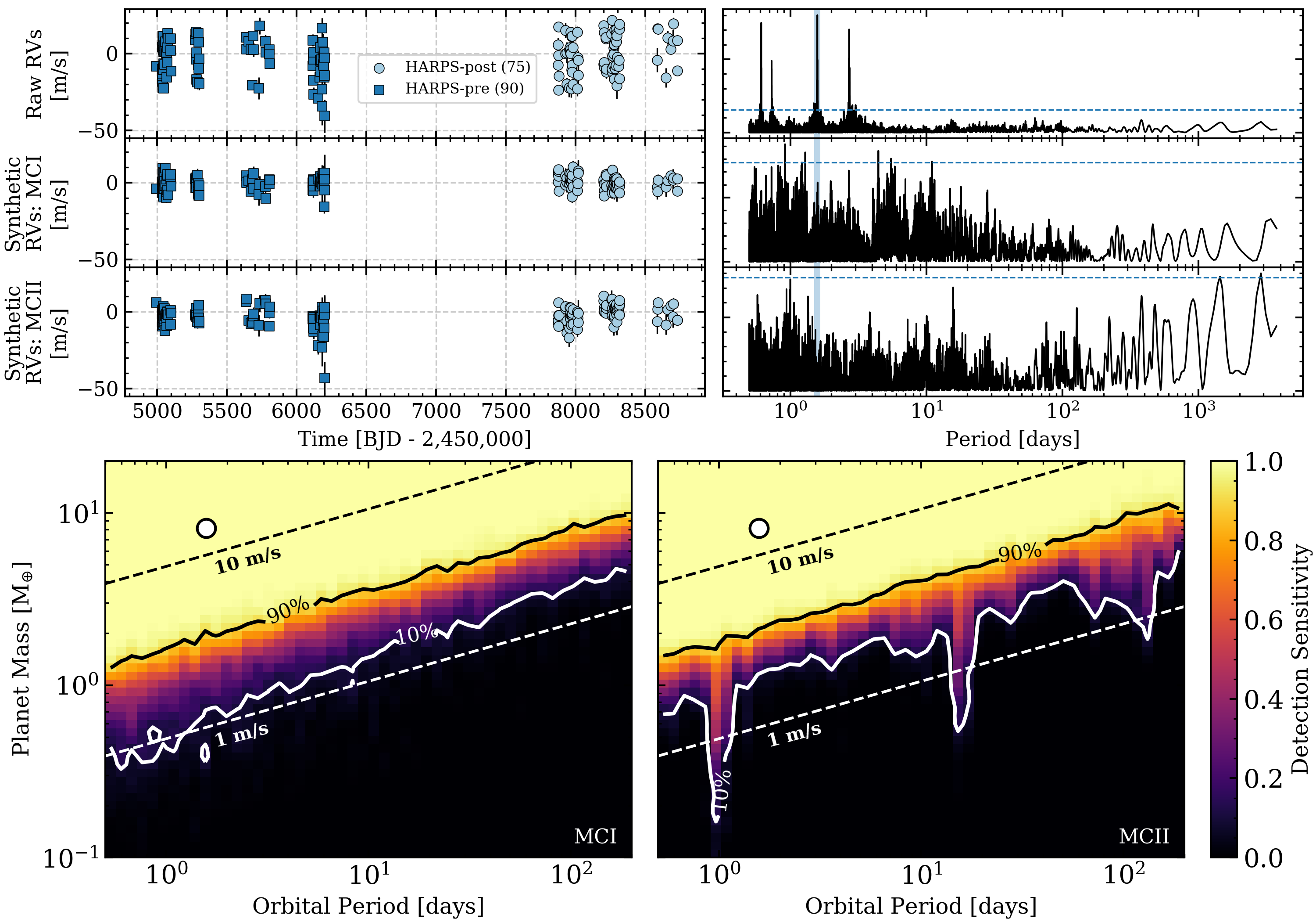
Figure 10: Raw and synthetic RVs time series, GLS periodograms, and sensitivity maps for GJ 1214. Top row: raw RV data from HARPS with 90 pre (squares) and 75 (circles) post-fiber upgrade measurements. Second row: an example of a noisy synthetic RV dataset from the Monte-Carlo simulation MCI wherein the noisy RVs are constructed from Gaussian noise with a dispersion equal to the rms of the RV residuals. Third row: noisy synthetic RV data from the Monte-Carlo simulation MCII wherein the noisy RVs are constructed from the RV residuals after the removal of GJ 1214 b only (i.e. no GP component is removed). Right column: each RV time series’ corresponding GLS periodogram. The vertical shaded regions highlight the orbital period of the planet GJ 1214 b ($P=1.58$ days). The horizontal dashed lines depict the approximate 1% FAP levels. Lower left panel: the RV detection sensitivity computed from MCI as a function of planet mass and orbital period. Lower right panel: the RV detection sensitivity from MCII. GJ 1214 b is depicted as a white circle marker in both panels. The solid contours highlight the 10% and 90% sensitivity levels. The dashed lines represent lines of constant semiamplitude with illustrative values equal to 1 and 10 m s^-1.

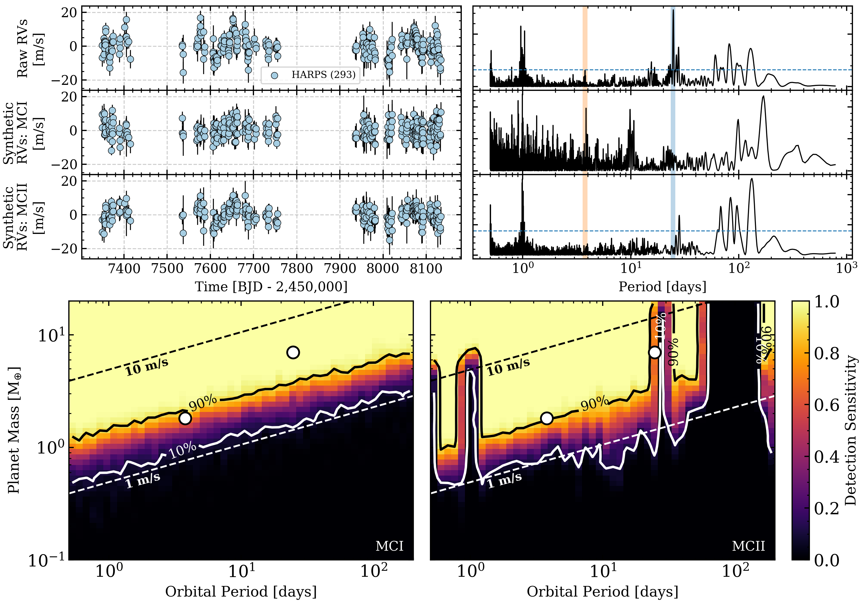
Figure 11: Similar to Figure 10 but for the LHS 1140 transiting system using RV data from HARPS (Ment et al., 2019).

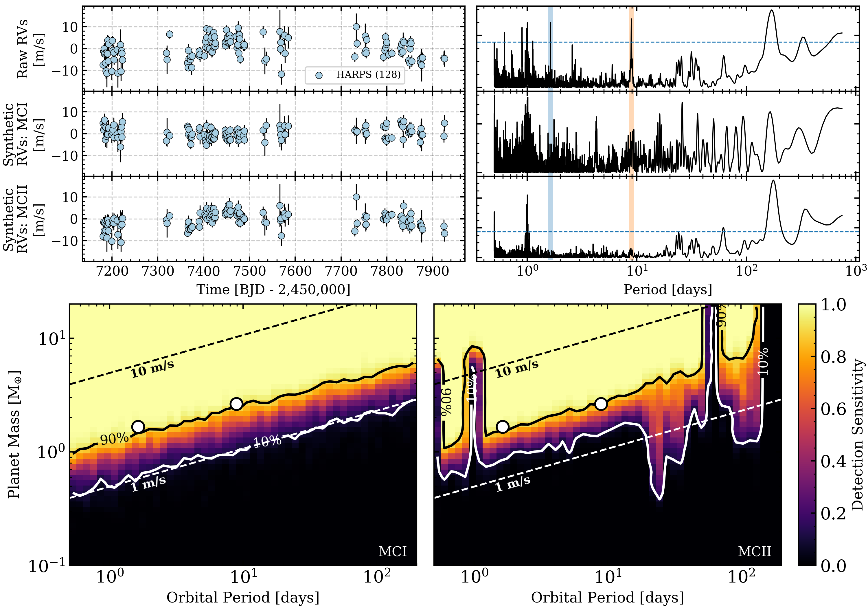
Figure 12: Similar to Figure 10 but for the GJ 1132 transiting system using RV data from HARPS (Bonfils et al., 2018b).

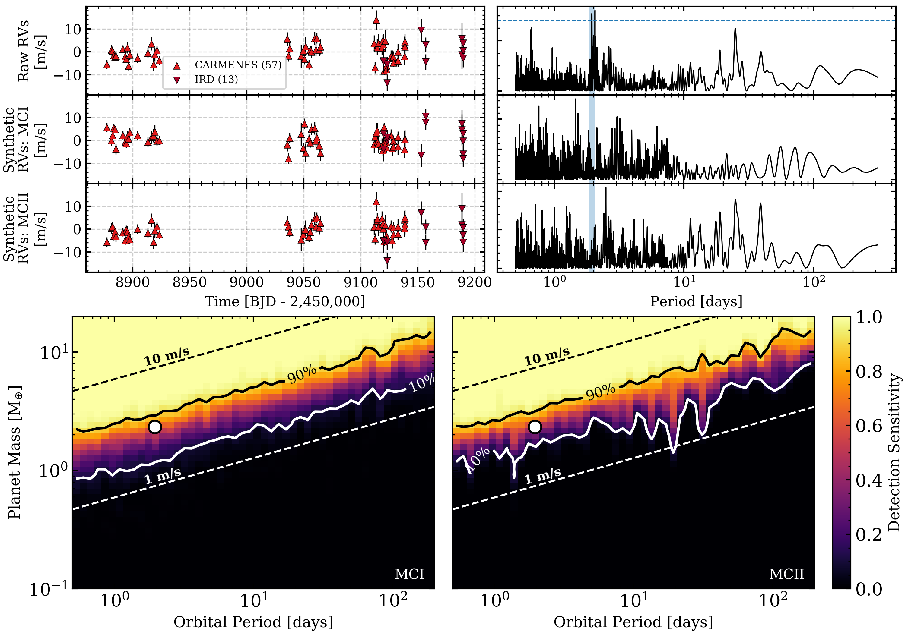
Figure 13: Similar to Figure 10 but for the LHS 1478 transiting system using RV data from CARMENES and IRD (Soto et al., 2021).

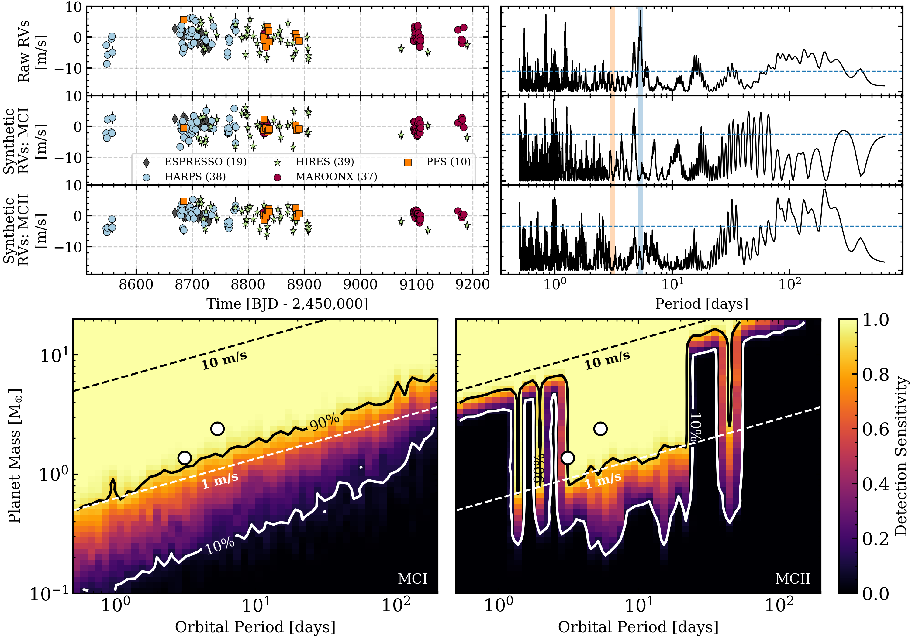
Figure 14: Similar to Figure 10 but for the LTT 1445 A transiting system using RV data from ESPRESSO, HARPS, HIRES, MAROON-X, and PFS (Winters et al. 2021 submitted).

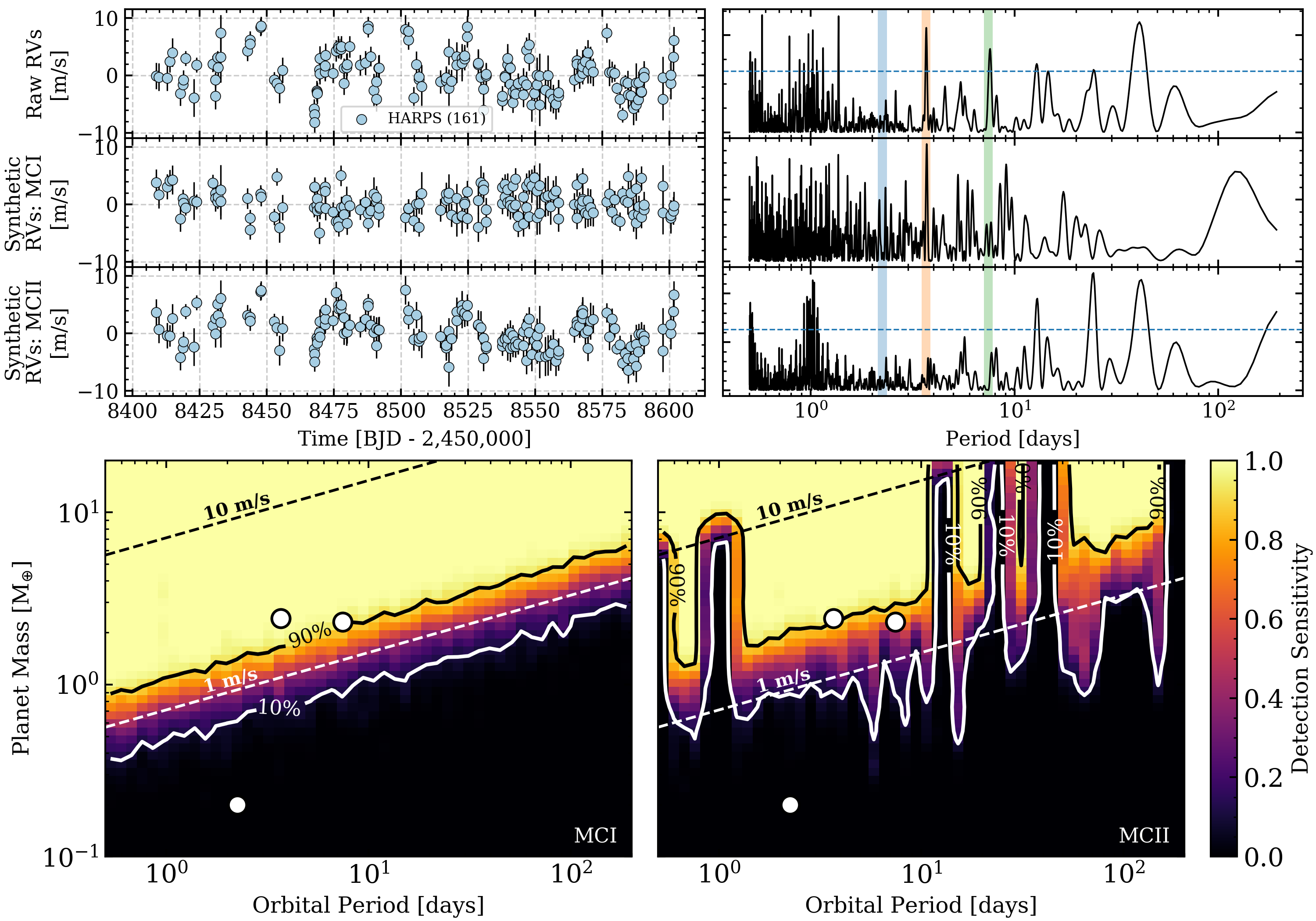
Figure 15: Similar to Figure 10 but for the L 98-59 transiting system using RV data from HARPS (Cloutier et al., 2019).

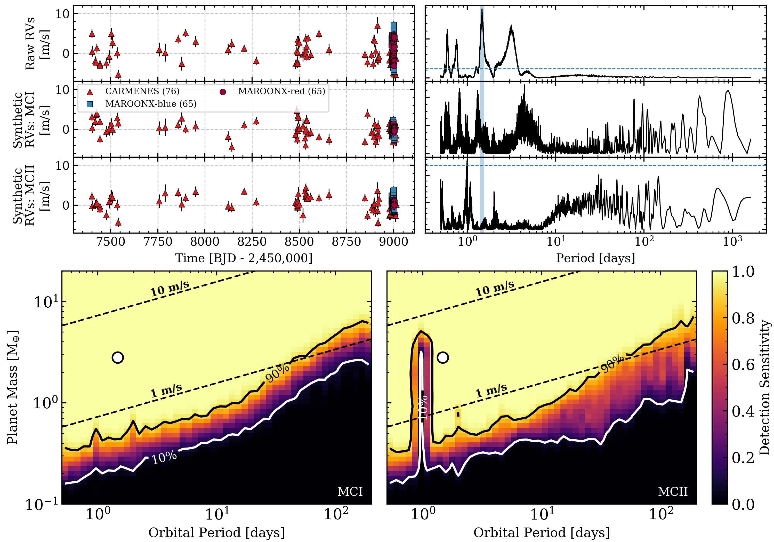
Figure 16: Similar to Figure 10 but for the GJ 486 transiting system using RV data from CARMENES, MAROON-X blue, and MAROON-X red (Trifonov et al., 2021).

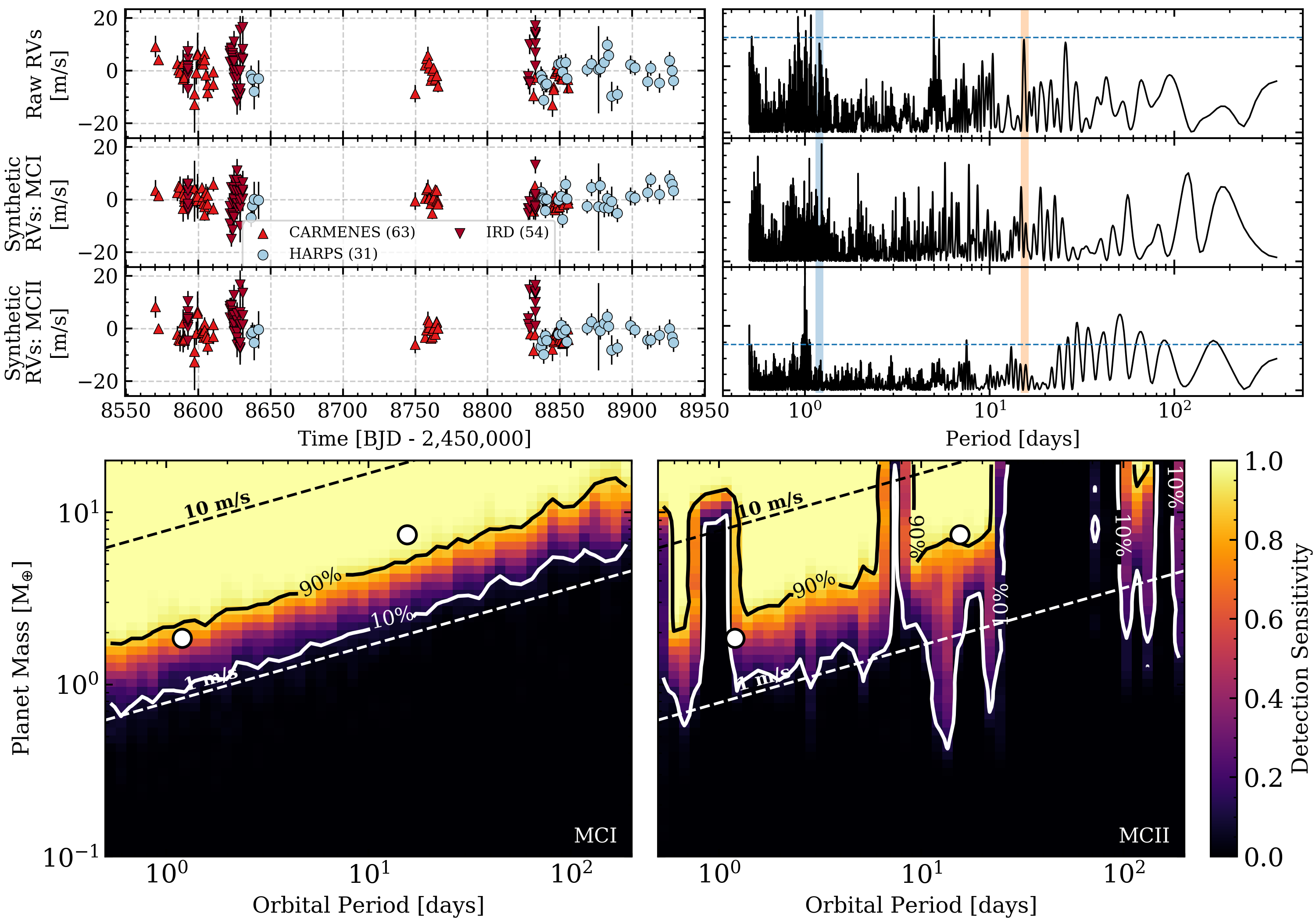
Figure 17: Similar to Figure 10 but for the GJ 3473 transiting system using RV data from CARMENES, HARPS, and IRD (Kemmer et al., 2020).

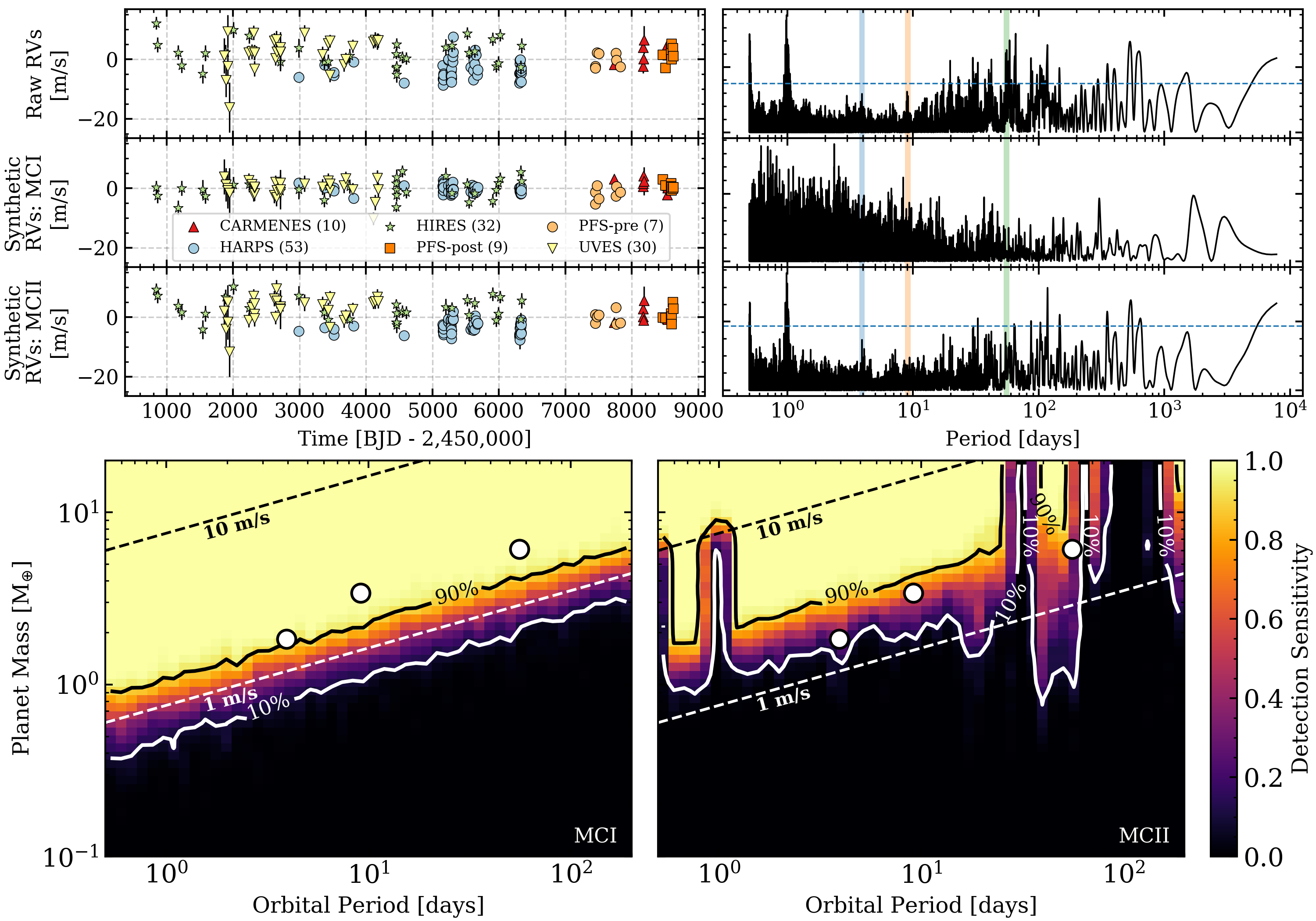
Figure 18: Similar to Figure 10 but for the GJ 357 transiting system using RV data from CARMENES, HARPS, HIRES, PFS (with two distinct iodine calibrations), and UVES (Luque et al., 2019).

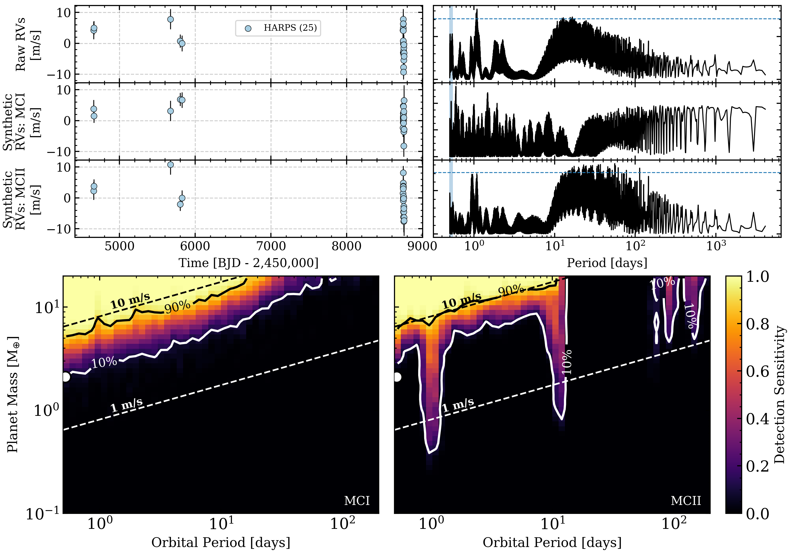
Figure 19: Similar to Figure 10 but for the GJ 1252 transiting system using RV data from HARPS (Shporer et al., 2020).

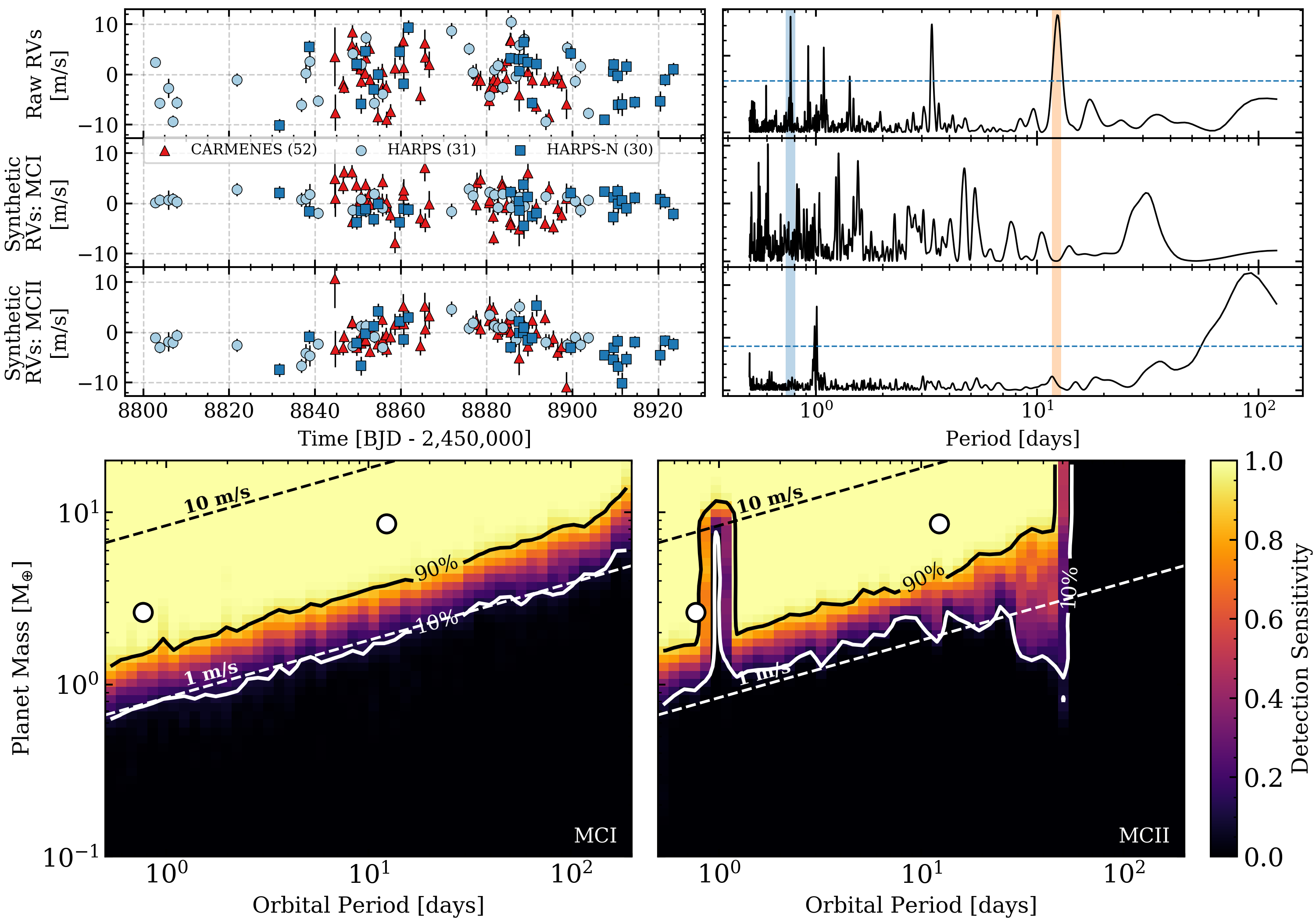
Figure 20: Similar to Figure 10 but for the LTT 3780 transiting system using RV data from CARMENES (Nowak et al., 2020), HARPS, and HARPS-N (Cloutier et al., 2020a).

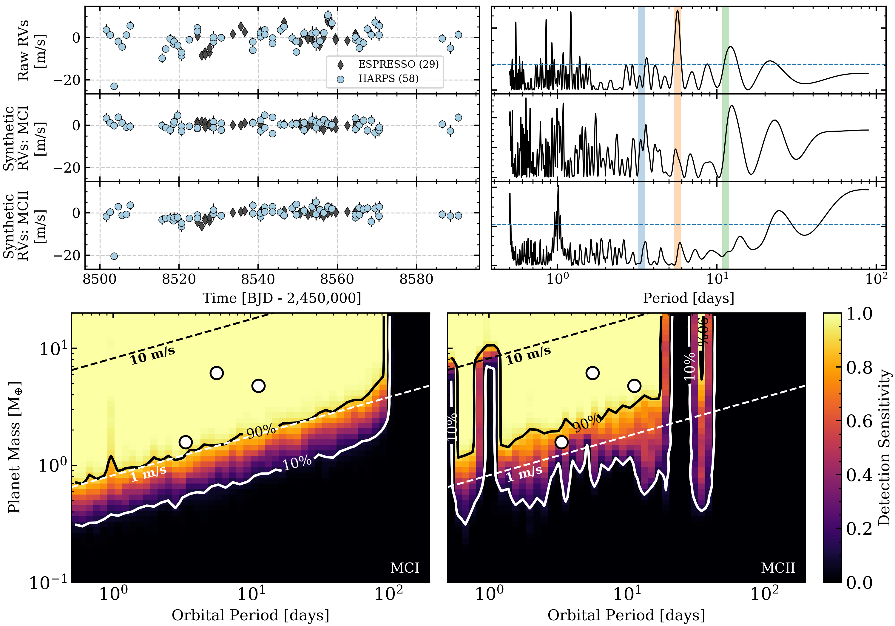
Figure 21: Similar to Figure 10 but for the TOI-270 transiting system using RV data from ESPRESSO and HARPS (Van Eylen et al., 2021).

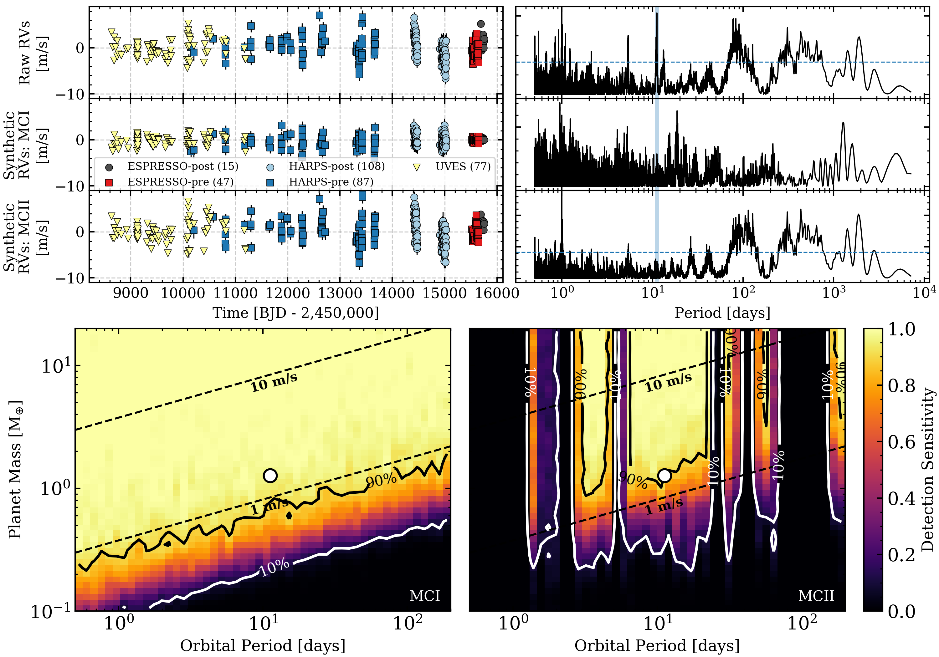
Figure 22: Similar to Figure 10 but for the Proxima Centauri RV system using RV data from ESPRESSO (Suárez Mascareño et al., 2020), HARPS and UVES (Anglada-Escudé et al., 2016).

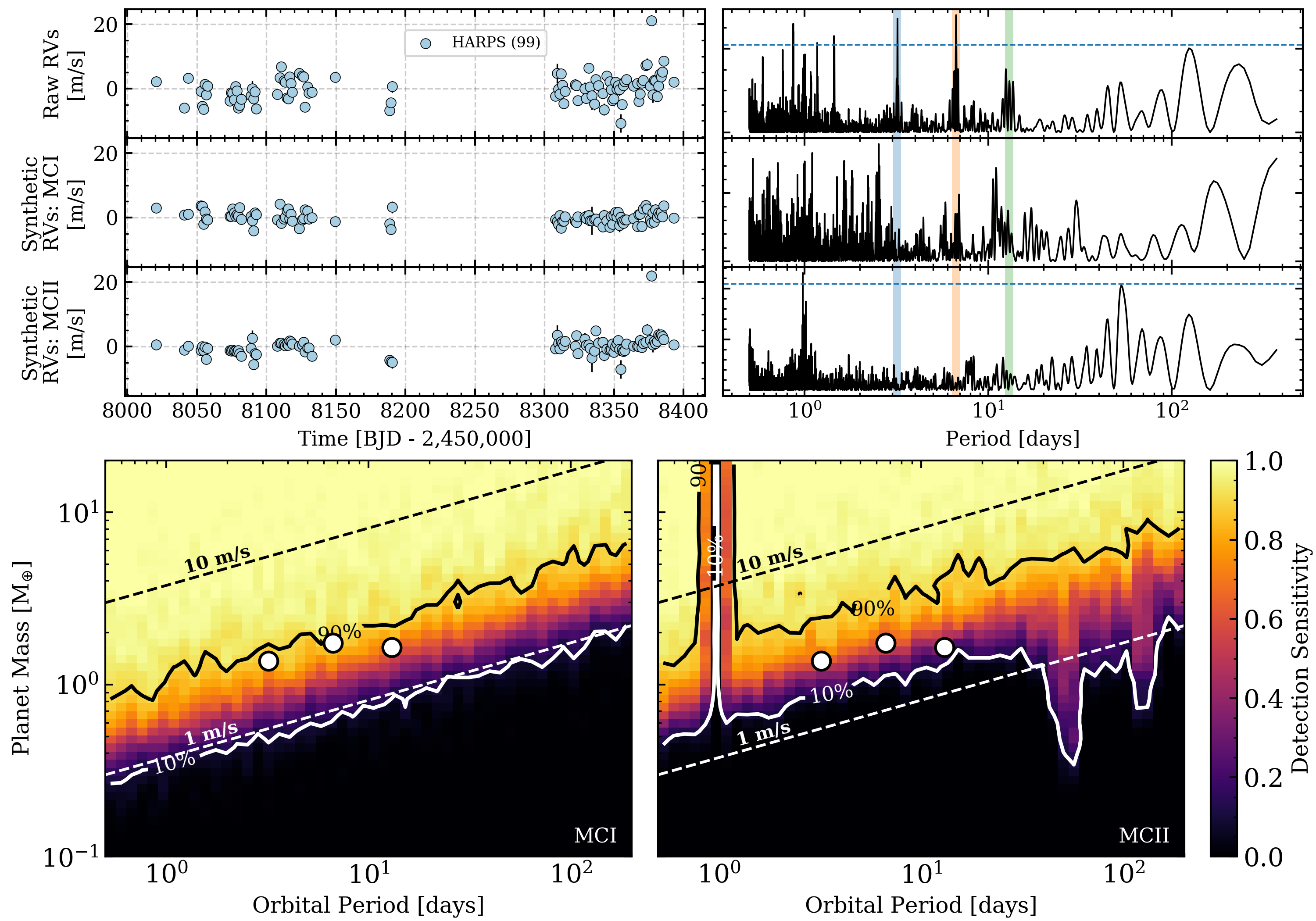
Figure 23: Similar to Figure 10 but for the GJ 1061 RV system using RV data from HARPS (Dreizler et al., 2020).

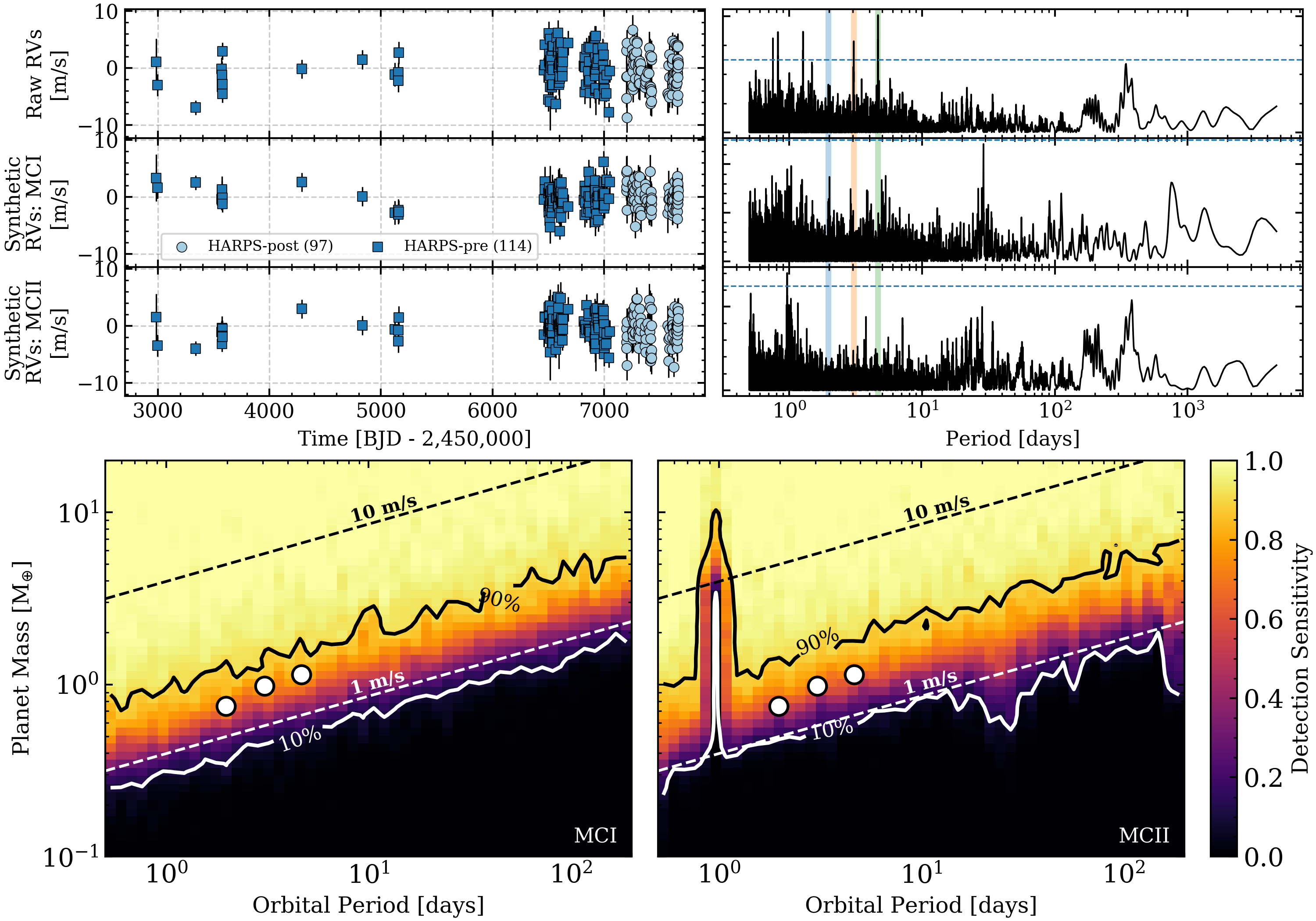
Figure 24: Similar to Figure 10 but for the YZ Ceti RV system using RV data from HARPS (Astudillo-Defru et al., 2017b).

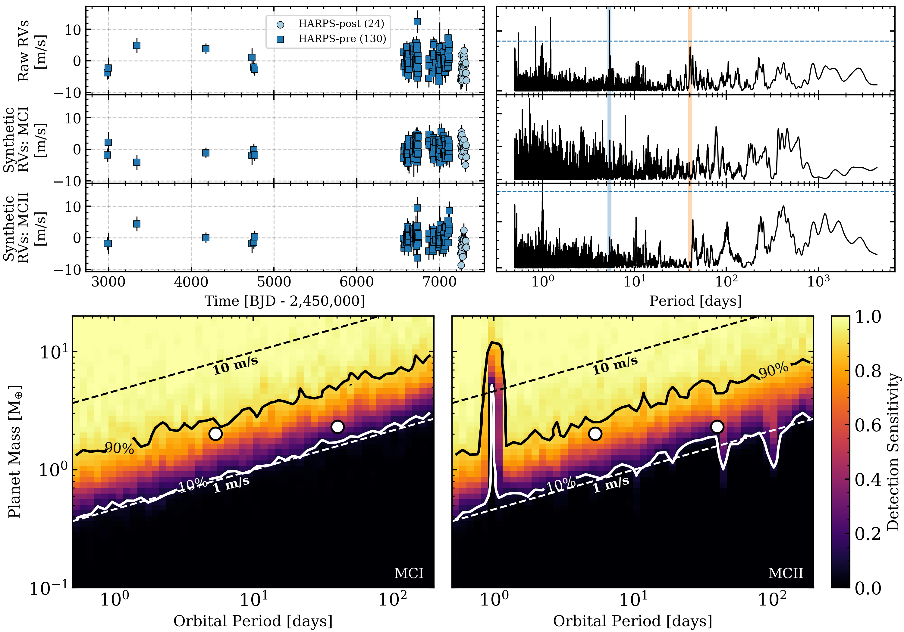
Figure 25: Similar to Figure 10 but for the GJ 3323 RV system using RV data from HARPS (Astudillo-Defru et al., 2017a).

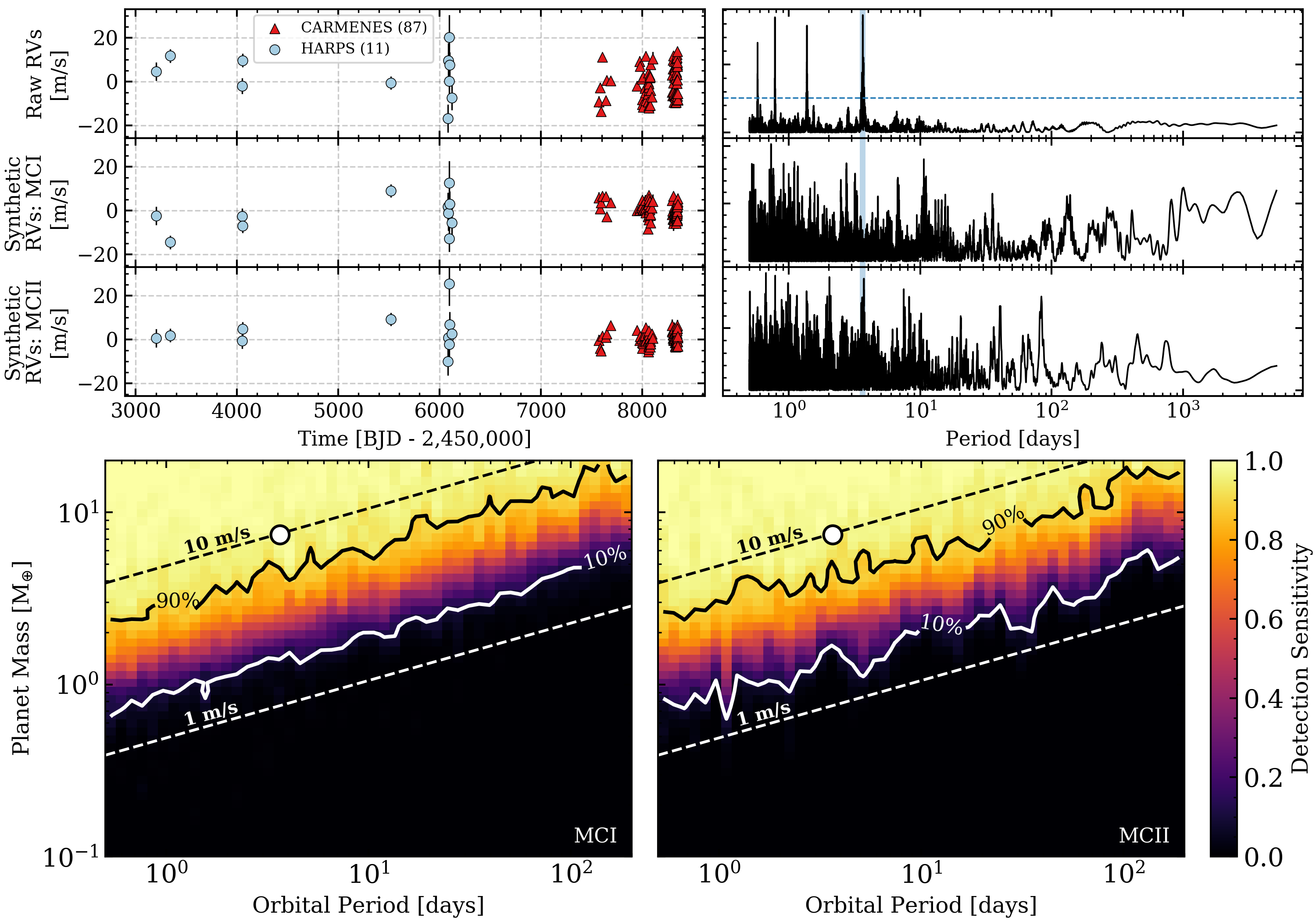
Figure 26: Similar to Figure 10 but for the GJ 1265 RV system using RV data from CARMENES and HARPS (Luque et al., 2018).

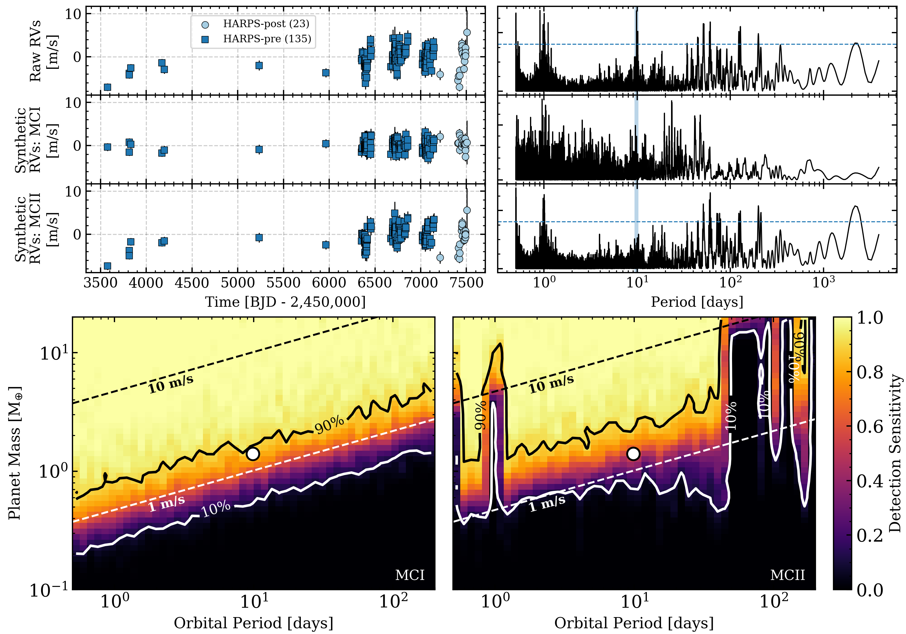
Figure 27: Similar to Figure 10 but for the Ross 128 RV system using RV data from HARPS (Bonfils et al., 2018a).

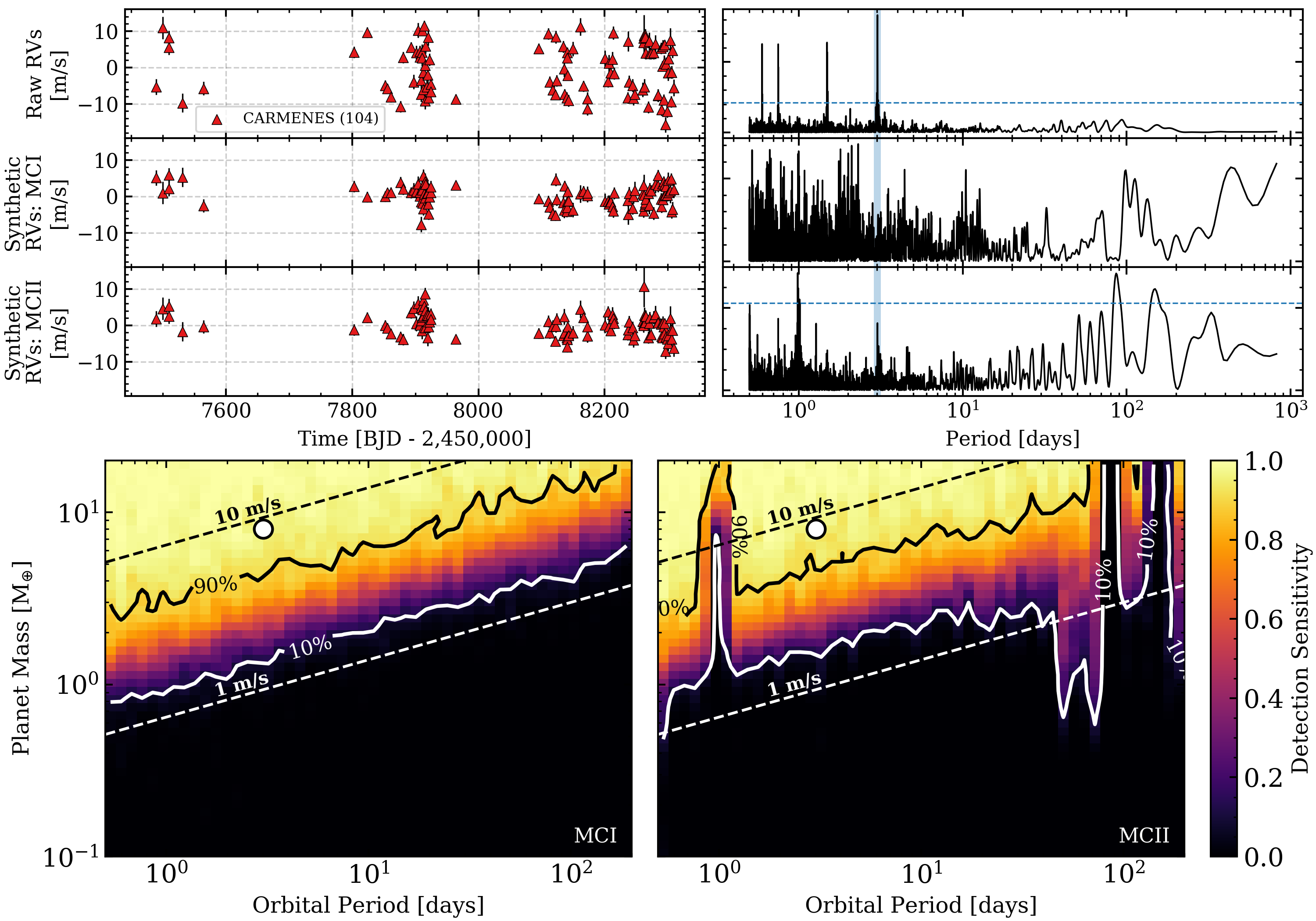
Figure 28: Similar to Figure 10 but for the GJ 3779 RV system using RV data from CARMENES (Luque et al., 2018).

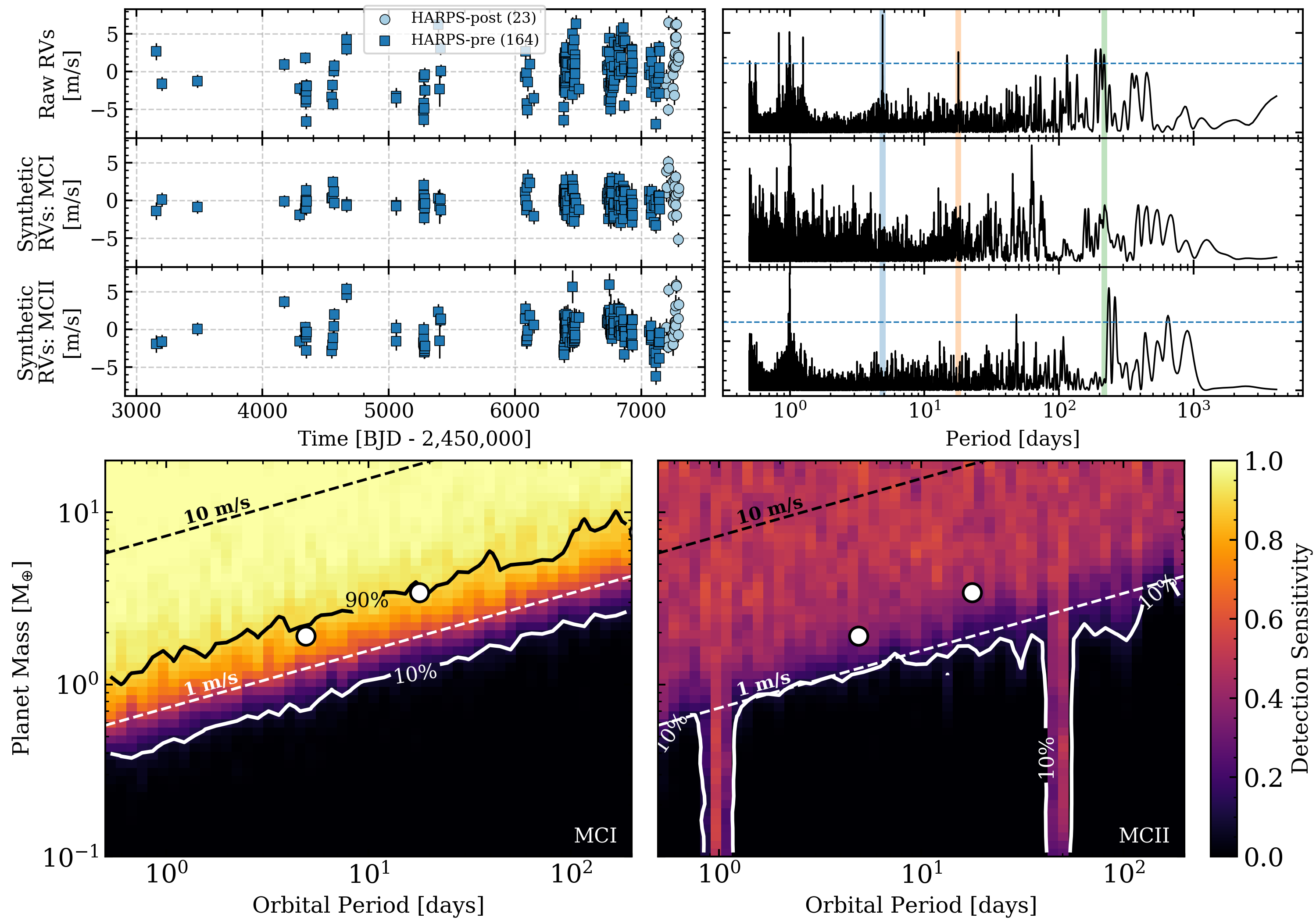
Figure 29: Similar to Figure 10 but for the Wolf 1061 RV system using RV data from HARPS (Astudillo-Defru et al., 2017a).

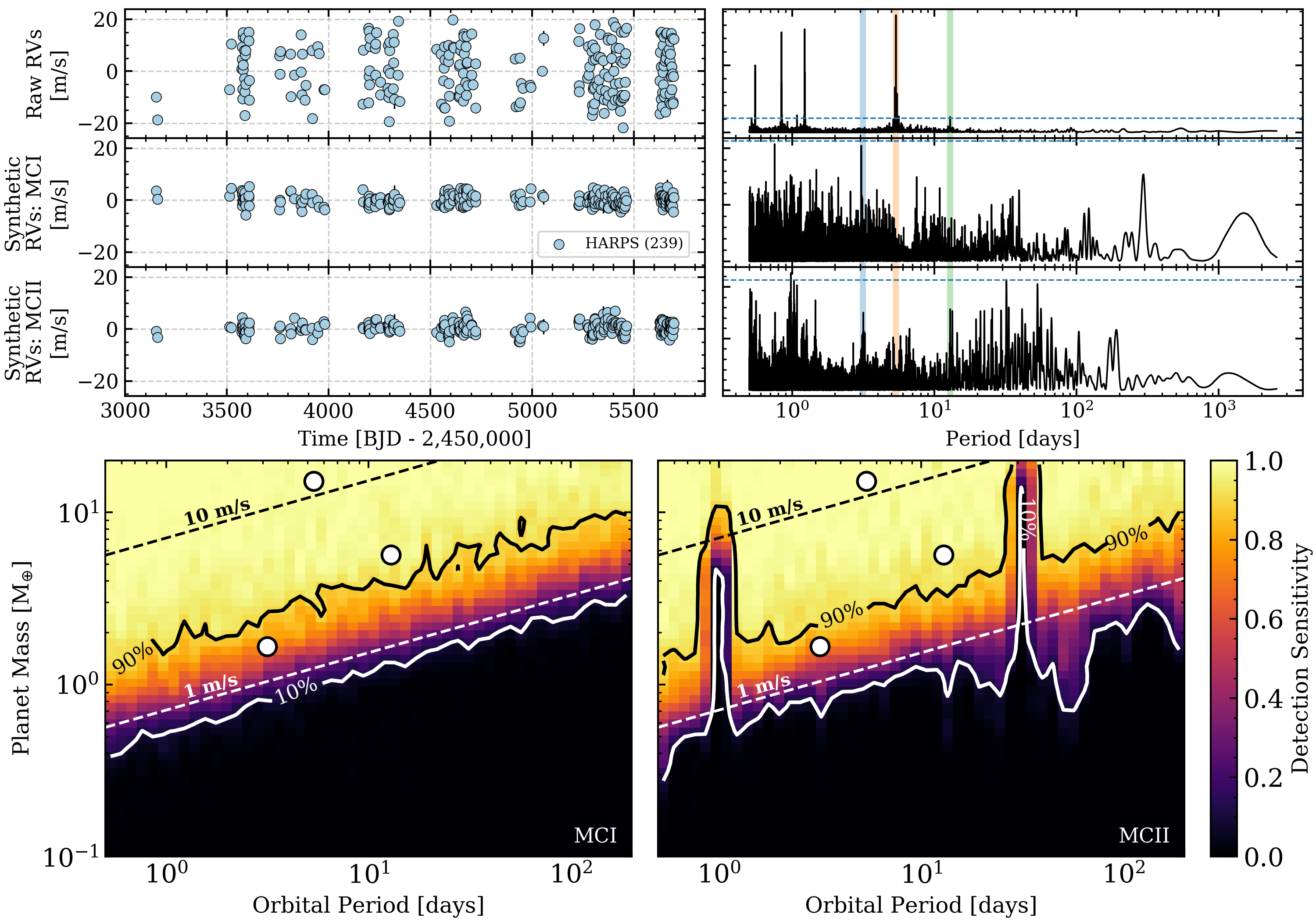
Figure 30: Similar to Figure 10 but for the GJ 581 RV system using RV data from HARPS (Trifonov et al., 2018).

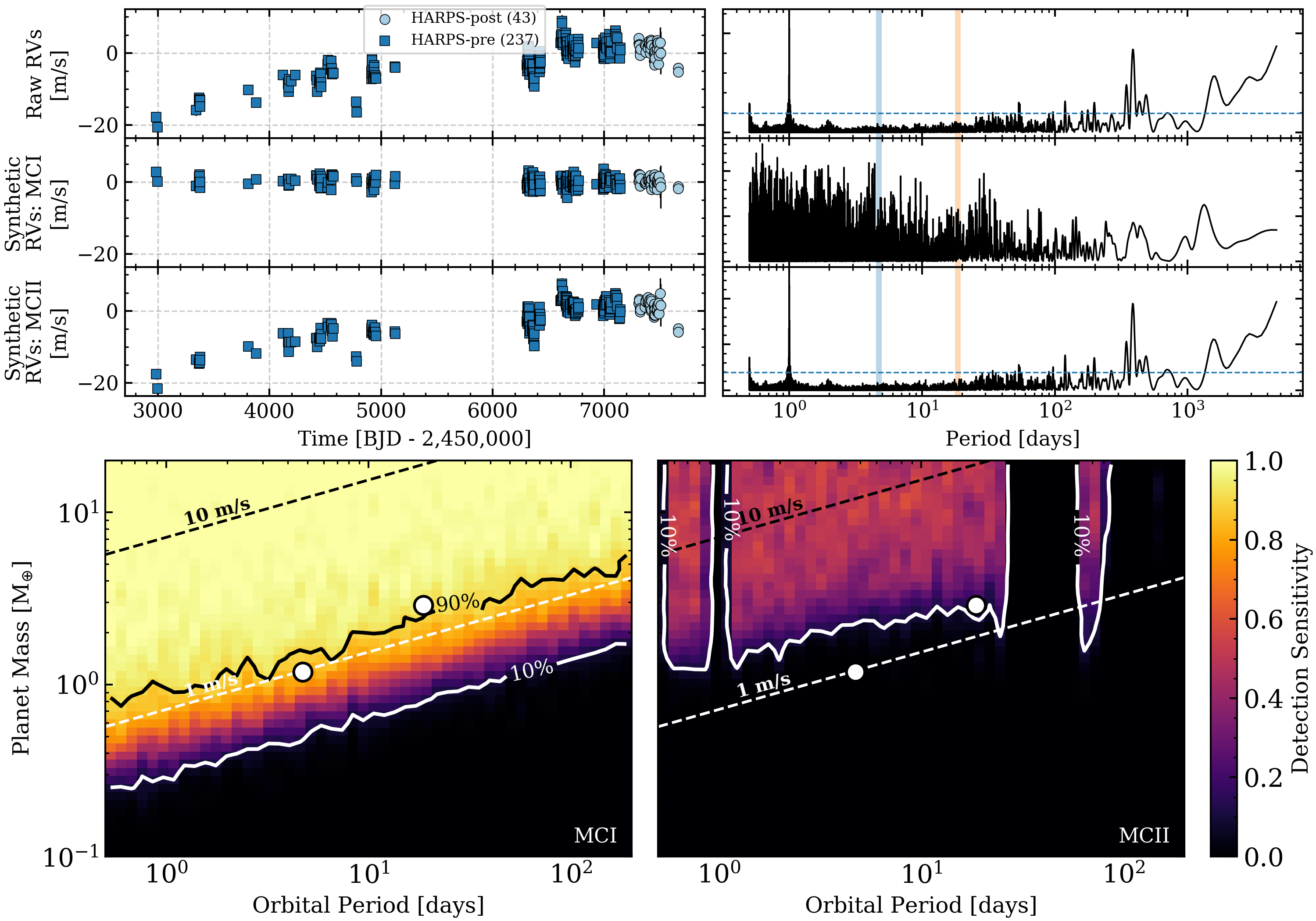
Figure 31: Similar to Figure 10 but for the GJ 273 RV system using RV data from HARPS (Astudillo-Defru et al., 2017a).

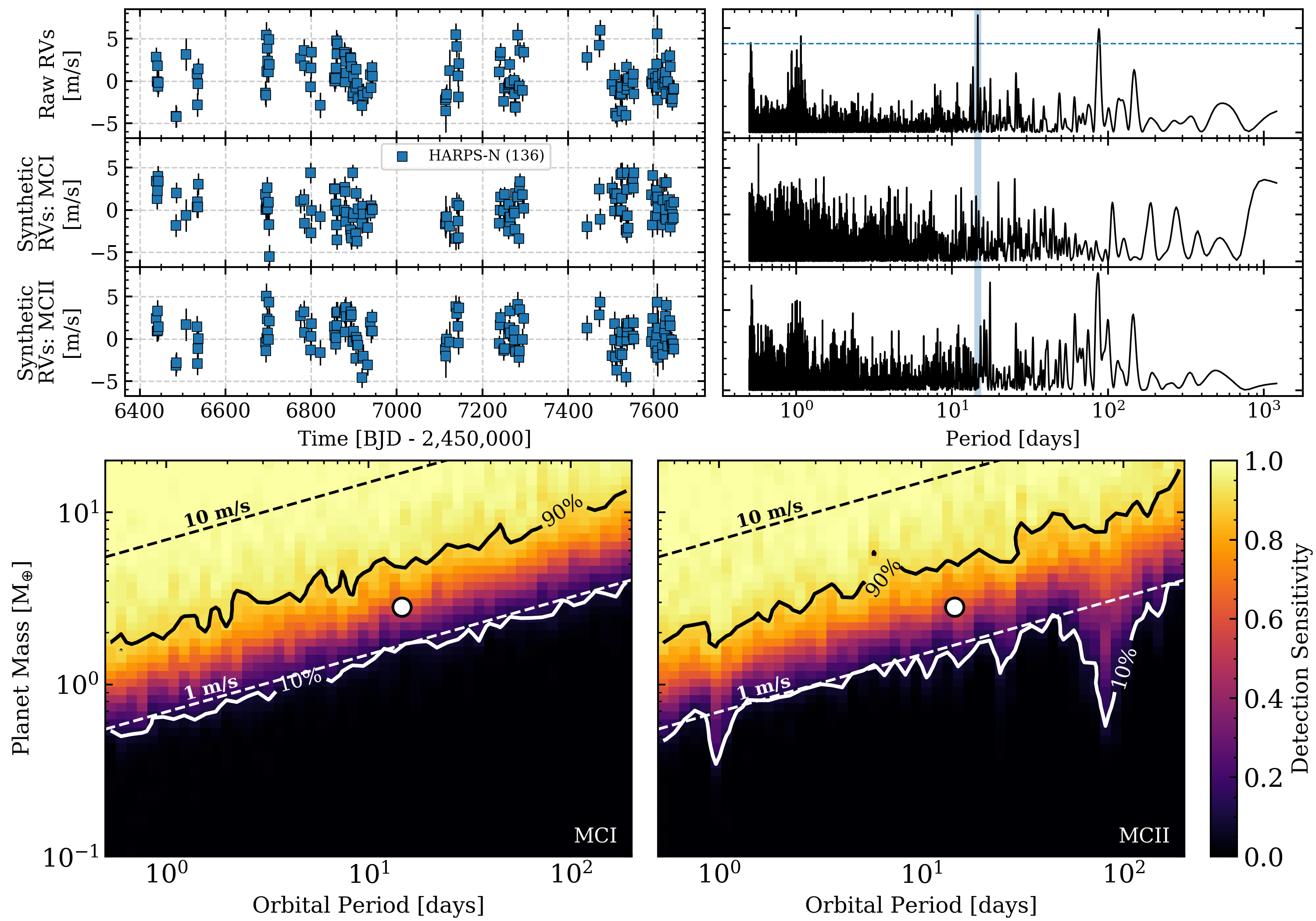
Figure 32: Similar to Figure 10 but for the GJ 625 RV system using RV data from HARPS (Suárez Mascareño et al., 2017).

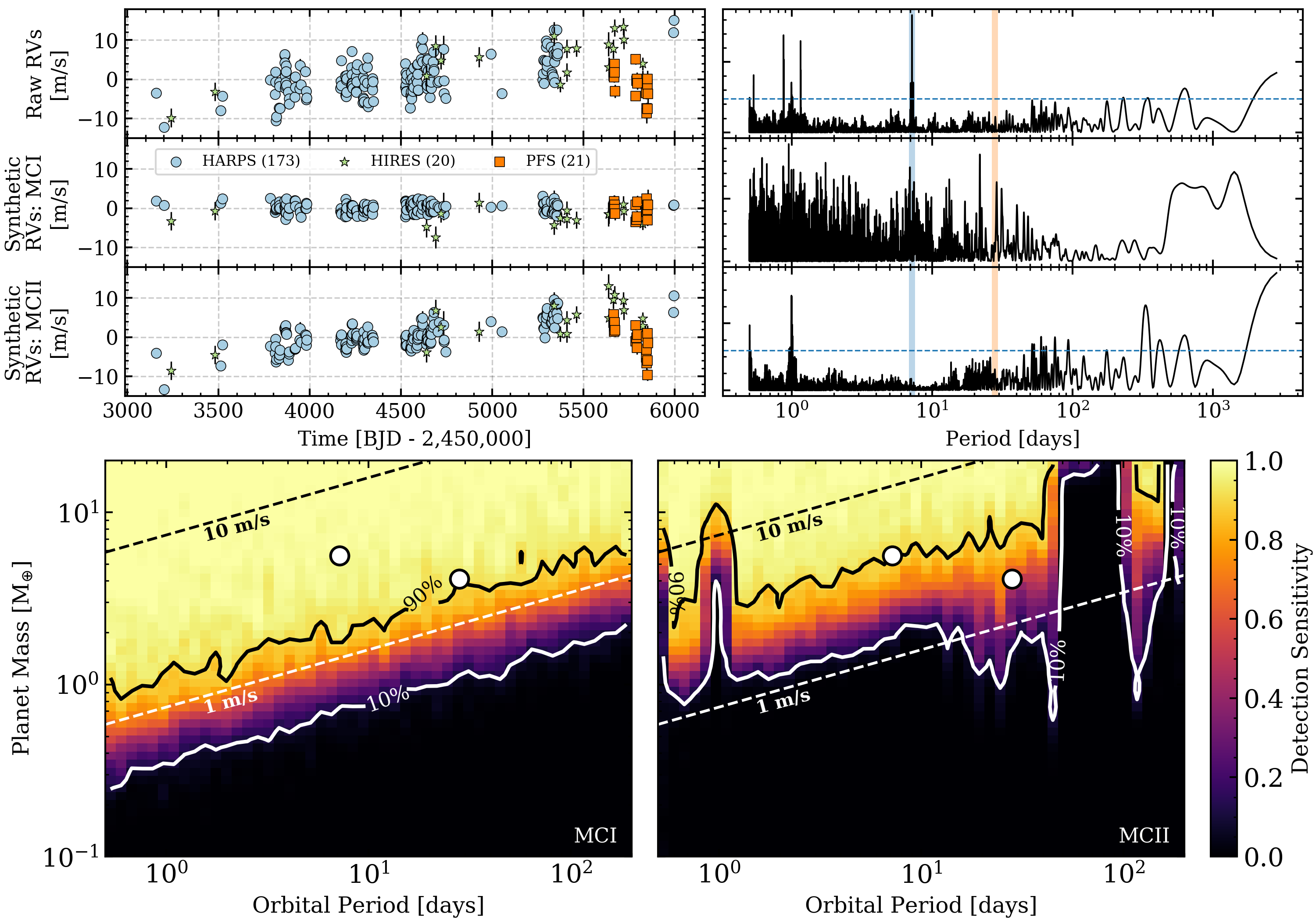
Figure 33: Similar to Figure 10 but for the GJ 667C RV system using RV data from HARPS, HIRES, and PFS (Anglada-Escudé et al., 2013b).

References

- Anglada-Escudé & Butler (2012) Anglada-Escudé, G., & Butler, R. P. 2012, ApJS, 200, 15
- Anglada-Escudé et al. (2013a) Anglada-Escudé, G., Rojas-Ayala, B., Boss, A. P., Weinberger, A. J., & Lloyd, J. P. 2013a, A&A, 551, A48
- Anglada-Escudé et al. (2013b) Anglada-Escudé, G., Tuomi, M., Gerlach, E., et al. 2013b, A&A, 556, A126
- Anglada-Escudé et al. (2016) Anglada-Escudé, G., Amado, P. J., Barnes, J., et al. 2016, Nature, 536, 437
- Astropy Collaboration et al. (2013) Astropy Collaboration, Robitaille, T. P., Tollerud, E. J., et al. 2013, A&A, 558, A33
- Astropy Collaboration et al. (2018) Astropy Collaboration, Price-Whelan, A. M., Sipőcz, B. M., et al. 2018, AJ, 156, 123
- Astudillo-Defru et al. (2015) Astudillo-Defru, N., Bonfils, X., Delfosse, X., et al. 2015, A&A, 575, A119
- Astudillo-Defru et al. (2017a) Astudillo-Defru, N., Forveille, T., Bonfils, X., et al. 2017a, A&A, 602, A88
- Astudillo-Defru et al. (2017b) Astudillo-Defru, N., Díaz, R. F., Bonfils, X., et al. 2017b, A&A, 605, L11
- Bailer-Jones et al. (2021) Bailer-Jones, C. A. L., Rybizki, J., Fouesneau, M., Demleitner, M., & Andrae, R. 2021, AJ, 161, 147
- Ballard & Johnson (2016) Ballard, S., & Johnson, J. A. 2016, ApJ, 816, 66
- Bean et al. (2011) Bean, J. L., Désert, J.-M., Kabath, P., et al. 2011, ApJ, 743, 92
- Benedict et al. (2016) Benedict, G. F., Henry, T. J., Franz, O. G., et al. 2016, AJ, 152, 141
- Berta et al. (2011) Berta, Z. K., Charbonneau, D., Bean, J., et al. 2011, ApJ, 736, 12
- Bonfils et al. (2018a) Bonfils, X., Astudillo-Defru, N., Díaz, R., et al. 2018a, A&A, 613, A25
- Bonfils et al. (2018b) Bonfils, X., Almenara, J.-M., Cloutier, R., et al. 2018b, A&A, 618, A142
- Carter et al. (2011) Carter, J. A., Winn, J. N., Holman, M. J., et al. 2011, ApJ, 730, 82
- Charbonneau et al. (2009) Charbonneau, D., Berta, Z. K., Irwin, J., et al. 2009, Nature, 462, 891
- Claret et al. (2012) Claret, A., Hauschildt, P. H., & Witte, S. 2012, A&A, 546, A14
- Cloutier et al. (2018) Cloutier, R., Doyon, R., Bouchy, F., & Hébrard, G. 2018, AJ, 156, 82
- Cloutier & Menou (2020) Cloutier, R., & Menou, K. 2020, AJ, 159, 211
- Cloutier et al. (2019) Cloutier, R., Astudillo-Defru, N., Bonfils, X., et al. 2019, A&A, 629, A111
- Cloutier et al. (2020a) Cloutier, R., Eastman, J. D., Rodriguez, J. E., et al. 2020a, AJ, 160, 3
- Cloutier et al. (2020b) Cloutier, R., Rodriguez, J. E., Irwin, J., et al. 2020b, AJ, 160, 22
- Croll et al. (2011) Croll, B., Albert, L., Jayawardhana, R., et al. 2011, ApJ, 736, 78
- Crossfield et al. (2011) Crossfield, I. J. M., Barman, T., & Hansen, B. M. S. 2011, ApJ, 736, 132
- Crossfield et al. (2019) Crossfield, I. J. M., Waalkes, W., Newton, E. R., et al. 2019, ApJ, 883, L16
- Cumming (2004) Cumming, A. 2004, MNRAS, 354, 1165
- Cumming et al. (1999) Cumming, A., Marcy, G. W., & Butler, R. P. 1999, ApJ, 526, 890
- Dai et al. (2018) Dai, F., Masuda, K., & Winn, J. N. 2018, ApJ, 864, L38
- Damasso et al. (2020) Damasso, M., Del Sordo, F., Anglada-Escudé, G., et al. 2020, Science Advances, 6, eaax7467
- Dawson & Johnson (2012) Dawson, R. I., & Johnson, J. A. 2012, ApJ, 756, 122
- de Mooij et al. (2012) de Mooij, E. J. W., Brogi, M., de Kok, R. J., et al. 2012, A&A, 538, A46
- Deming et al. (2015) Deming, D., Knutson, H., Kammer, J., et al. 2015, ApJ, 805, 132
- Díaz et al. (2019) Díaz, R. F., Delfosse, X., Hobson, M. J., et al. 2019, A&A, 625, A17
- Dreizler et al. (2020) Dreizler, S., Jeffers, S. V., Rodríguez, E., et al. 2020, MNRAS, 493, 536
- Dressing & Charbonneau (2015) Dressing, C. D., & Charbonneau, D. 2015, ApJ, 807, 45
- Eastman et al. (2013) Eastman, J., Gaudi, B. S., & Agol, E. 2013, PASP, 125, 83
- Fazio et al. (2004) Fazio, G. G., Hora, J. L., Allen, L. E., et al. 2004, ApJS, 154, 10
- Foreman-Mackey et al. (2017) Foreman-Mackey, D., Agol, E., Ambikasaran, S., & Angus, R. 2017, AJ, 154, 220
- Foreman-Mackey et al. (2013) Foreman-Mackey, D., Hogg, D. W., Lang, D., & Goodman, J. 2013, PASP, 125, 306
- Fraine et al. (2013) Fraine, J. D., Deming, D., Gillon, M., et al. 2013, ApJ, 765, 127
- Gaidos et al. (2016) Gaidos, E., Mann, A. W., Kraus, A. L., & Ireland, M. 2016, MNRAS, 457, 2877
- Garhart et al. (2020) Garhart, E., Deming, D., Mandell, A., et al. 2020, AJ, 159, 137
- Gaudi & Winn (2007) Gaudi, B. S., & Winn, J. N. 2007, ApJ, 655, 550
- Gillon et al. (2014) Gillon, M., Demory, B. O., Madhusudhan, N., et al. 2014, A&A, 563, A21
- Gupta & Schlichting (2019) Gupta, A., & Schlichting, H. E. 2019, MNRAS, 487, 24
- Hamann et al. (2019) Hamann, A., Montet, B. T., Fabrycky, D. C., Agol, E., & Kruse, E. 2019, AJ, 158, 133
- Hardegree-Ullman et al. (2019) Hardegree-Ullman, K. K., Cushing, M. C., Muirhead, P. S., & Christiansen, J. L. 2019, AJ, 158, 75
- Harpsøe et al. (2013) Harpsøe, K. B. W., Hardis, S., Hinse, T. C., et al. 2013, A&A, 549, A10
- Haywood et al. (2014) Haywood, R. D., Collier Cameron, A., Queloz, D., et al. 2014, MNRAS, 443, 2517
- Hirano et al. (2018) Hirano, T., Dai, F., Gandolfi, D., et al. 2018, AJ, 155, 127
- Hsu et al. (2020) Hsu, D. C., Ford, E. B., & Terrien, R. 2020, MNRAS, 498, 2249
- Kemmer et al. (2020) Kemmer, J., Stock, S., Kossakowski, D., et al. 2020, A&A, 642, A236
- Kopparapu et al. (2013) Kopparapu, R. K., Ramirez, R., Kasting, J. F., et al. 2013, ApJ, 765, 131
- Kreidberg (2015) Kreidberg, L. 2015, PASP, 127, 1161
- Kreidberg et al. (2014) Kreidberg, L., Bean, J. L., Désert, J.-M., et al. 2014, Nature, 505, 69
- Lalitha et al. (2014) Lalitha, S., Poppenhaeger, K., Singh, K. P., Czesla, S., & Schmitt, J. H. M. M. 2014, ApJ, 790, L11
- Lillo-Box et al. (2020) Lillo-Box, J., Figueira, P., Leleu, A., et al. 2020, A&A, 642, A121
- Lindegren et al. (2021) Lindegren, L., Klioner, S. A., Hernández, J., et al. 2021, A&A, 649, A2
- Lo Curto et al. (2015) Lo Curto, G., Pepe, F., Avila, G., et al. 2015, The Messenger, 162, 9
- Lovis & Pepe (2007) Lovis, C., & Pepe, F. 2007, A&A, 468, 1115
- Lubin et al. (2021) Lubin, J., Robertson, P., Stefansson, G., et al. 2021, arXiv e-prints, arXiv:2105.07005
- Lucy & Sweeney (1971) Lucy, L. B., & Sweeney, M. A. 1971, AJ, 76, 544
- Luque et al. (2018) Luque, R., Nowak, G., Pallé, E., et al. 2018, A&A, 620, A171
- Luque et al. (2019) Luque, R., Pallé, E., Kossakowski, D., et al. 2019, A&A, 628, A39
- Mallonn et al. (2018) Mallonn, M., Herrero, E., Juvan, I. G., et al. 2018, A&A, 614, A35
- Mandel & Agol (2002) Mandel, K., & Agol, E. 2002, ApJL, 580, L171
- Mann et al. (2015) Mann, A. W., Feiden, G. A., Gaidos, E., Boyajian, T., & von Braun, K. 2015, ApJ, 804, 64
- Marcus et al. (2010) Marcus, R. A., Sasselov, D., Hernquist, L., & Stewart, S. T. 2010, ApJ, 712, L73
- Mayor et al. (2003) Mayor, M., Pepe, F., Queloz, D., et al. 2003, The Messenger, 114, 20
- Ment et al. (2019) Ment, K., Dittmann, J. A., Astudillo-Defru, N., et al. 2019, AJ, 157, 32
- Moorhead et al. (2011) Moorhead, A. V., Ford, E. B., Morehead, R. C., et al. 2011, ApJS, 197, 1
- Muirhead et al. (2015) Muirhead, P. S., Mann, A. W., Vanderburg, A., et al. 2015, ApJ, 801, 18
- Narita et al. (2013) Narita, N., Fukui, A., Ikoma, M., et al. 2013, ApJ, 773, 144
- Nascimbeni et al. (2015) Nascimbeni, V., Mallonn, M., Scandariato, G., et al. 2015, A&A, 579, A113
- Nava et al. (2020) Nava, C., López-Morales, M., Haywood, R. D., & Giles, H. A. C. 2020, AJ, 159, 23
- Newton et al. (2014) Newton, E. R., Charbonneau, D., Irwin, J., et al. 2014, AJ, 147, 20
- Newton et al. (2016) Newton, E. R., Irwin, J., Charbonneau, D., Berta-Thompson, Z. K., & Dittmann, J. A. 2016, ApJ, 821, L19
- Nowak et al. (2020) Nowak, G., Luque, R., Parviainen, H., et al. 2020, A&A, 642, A173
- Owen & Wu (2017) Owen, J. E., & Wu, Y. 2017, ApJ, 847, 29
- Rackham et al. (2017) Rackham, B., Espinoza, N., Apai, D., et al. 2017, ApJ, 834, 151
- Rajpaul et al. (2016) Rajpaul, V., Aigrain, S., & Roberts, S. 2016, MNRAS, 456, L6
- Robertson & Mahadevan (2014) Robertson, P., & Mahadevan, S. 2014, ApJ, 793, L24
- Robertson et al. (2014) Robertson, P., Mahadevan, S., Endl, M., & Roy, A. 2014, Science, 345, 440
- Rogers & Owen (2021) Rogers, J. G., & Owen, J. E. 2021, MNRAS, 503, 1526
- Rojas-Ayala et al. (2012) Rojas-Ayala, B., Covey, K. R., Muirhead, P. S., & Lloyd, J. P. 2012, ApJ, 748, 93