Update on $|V_{us}|$ and $|V_{us}/V_{ud}|$ from semileptonic
kaon and pion decays

Abstract

Implications for Cabibbo universality based on progress in the study of semileptonic kaon and pion decays are discussed. Included are recent updates of experimental input along with improved radiative corrections, form factors and isospin breaking effects. As a result, we obtain for the Cabibbo-Kobayashi-Maskawa (CKM) quark mixing matrix element $|V_{us}|=0.22309(56)$ from semileptonic $K_{\ell 3}$ $(K\rightarrow\pi\ell\nu)$ decays and $|V_{us}/V_{ud}|=0.22908(87)$ from the ratio between the kaon and pion ($\pi_{e3}$) semileptonic decay rates. In both, a lattice QCD value of the form factor $|f_{+}^{K}(0)|=0.9698(17)$ is employed. The $V_{us}$ from $K_{\ell 3}$ decays together with $V_{ud}=0.97373(31)$ found from superallowed nuclear beta decays implies an apparent $3.2\sigma$ violation of the first-row CKM unitarity condition. The $|V_{us}|/|V_{ud}|$ obtained from the ratio of weak vector current induced meson decays is consistent with the observed unitarity violation but found to differ by $2.2\sigma$ from its extraction using the ratio of weak axial-vector leptonic decay rates $\Gamma(K\rightarrow\mu\nu)/\Gamma(\pi\rightarrow\mu\nu)$. The situation suggests a difference between vector and axial-vector derived CKM matrix elements or a problem with the lattice QCD form factor input. Prospects for future improvements in comparative precision tests involving $|V_{ud}|$, $|V_{us}|$ and their ratios are briefly described.

I Introduction

Precision tests of the Standard Model (SM) have become increasingly important given the null results from high-energy colliders in the search for physics beyond the Standard Model (BSM) Zyla et al. (2020). Deviation from expectations in the muon anomalous magnetic moment Abi et al. (2021); Aoyama et al. (2020); Miller et al. (2007, 2012); Jegerlehner and Nyffeler (2009), hints of lepton flavor universality violation in B decays Aaij et al. (2019, 2014, 2015, 2016) and tests of unitarity in the Cabibbo-Kobayashi-Maskawa (CKM) quark mixing matrix are all exhibiting potential BSM effects. In the last case, improvements in the electroweak radiative corrections (RCs) Seng et al. (2018, 2019); Czarnecki et al. (2019); Seng et al. (2020a); Hayen (2021a, b); Shiells et al. (2021); Seng (2021) have revealed tension in the first-row unitarity requirement $|V_{ud}|^{2}+|V_{us}|^{2}+|V_{ub}|^{2}=1$ Hardy and Towner (2020). Similarly, the difference in the value of $|V_{us}|$ extracted from $K_{\ell 3}$ and $K_{\mu 2}$ decays needs to be better understood. Possible explanations based on BSM calculations Bryman and Shrock (2019a, b); Kirk (2021); Grossman et al. (2020); Belfatto et al. (2020); Cheung et al. (2020); Jho et al. (2020); Yue and Cheng (2021); Endo and Mishima (2020); Capdevila et al. (2021); Eberhardt et al. (2021); Crivellin and Hoferichter (2020); Coutinho et al. (2020); Gonzalez-Alonso et al. (2019); Falkowski et al. (2019); Cirigliano et al. (2019a); Falkowski et al. (2021); Bečirević et al. (2021); Crivellin et al. (2021a); Tan (2019); Crivellin et al. (2021b); Crivellin et al. (2020); Crivellin et al. (2021c); Dekens et al. (2021); Belfatto and Berezhiani (2021) have been conjectured. The confirmation of such ideas will require improvements in both experiment and SM theory.

In this work, we focus on the extraction of $|V_{us}|$ from $K\rightarrow\pi\ell\nu$ semileptonic decay processes known as $K_{\ell 3}$. Our starting point is the comprehensive 2010 FlaviaNet Working Group Report Antonelli et al. (2010) which presented a thorough review of all relevant experimental and theoretical information available at the time. Since then, significant progress has been made on both the experimental and theoretical fronts, including new measurements of the $K_{S}$ lifetime Abouzaid et al. (2011); Ambrosino et al. (2011) and branching ratio (BR) Babusci et al. (2020), updates of the electroweak RCs Ma et al. (2021); Seng et al. (2021a, b), phase space factors Cirigliano et al. (2019b), $K\pi$ form factor and isospin-breaking corrections (Aoki et al. (2020) and references therein). Some of those advances have been more recently discussed by FlaviaNet Working Group members in the form of proceedings  Moulson (2017) and conference slides Passemar and Moulson (2018); Cirigliano et al. (2019b) rather than more detailed research publications, making cross-checking difficult. For that reason, we present in this paper an updated status report on the value of $|V_{us}|$ extracted from $K_{\ell 3}$ decay properties. With the recent theory progress, we find that apart from the lattice input of the $K\pi$ form factor which is a universal multiplicative constant, the experimental errors from the kaon lifetimes and BRs are by far the dominant sources of uncertainties in all six channels of $K_{\ell 3}$, which is quite different from the situation a few years ago, in particular before the new calculation of the $K_{e3}$ RC Seng et al. (2021a, b).

The progress described above can also be applied to the determination of the recently proposed ratio $R_{V}=\Gamma(K_{\ell 3})/\Gamma(\pi_{e3})$ as an alternative approach to study $|V_{us}/V_{ud}|$ Czarnecki et al. (2020), complementary to the existing method based on $R_{A}=\Gamma(K_{\mu 2})/\Gamma(\pi_{\mu 2})$. We show, following the recent improvements in the precision level of the $K_{e3}$ Seng et al. (2021a, b) and $\pi_{e3}$ RC Feng et al. (2020), that $R_{V}$ is now a theoretically cleaner observable than $R_{A}$. It provides strong motivation to further improve the experimental precision of the $\pi_{e3}$ BR and $K_{\ell 3}$ decay properties as much as possible. An experimental next-generation rare pion decay program proposal: PIONEER Hertzog (2021); Aguilar-Arevalo et al. would aim to improve the experimental $\pi_{e3}$ decay rate by a factor of 3 or better, making the $K_{\ell 3}$ decay rate the dominant uncertainty in $R_{V}$.

The paper is organized as follows: In Sec. II, we give a detailed update on $|V_{us}f_{+}^{K}(0)|$ and $|V_{us}|$. Similarly, Sec. III provides updates on $|V_{us}f_{+}^{K}(0)|/|V_{ud}f_{+}^{\pi}(0)|$ and $|V_{us}/V_{ud}|$. We end with conclusions in Sec. IV. Some technicalities are relegated to the Appendix.

II Updates on $|V_{us}f_{+}^{K}(0)|$ and $|V_{us}|$

We start from the quantity $|V_{us}f_{+}^{K}(0)|$, with $f_{+}^{K}(0)$ the vector form factor in the $K^{0}\to\pi^{-}$ transition at zero momentum transfer. It is extracted from $K_{\ell 3}$ decays through the following master formula Zyla et al. (2020):

$$A_{K\ell}\equiv|V_{us}f_{+}^{K}(0)|_{K\ell}=\sqrt{\frac{192\pi^{3}\mathrm{BR}(K\ell)\Gamma_{K}}{G_{F}^{2}M_{K}^{5}C_{K}^{2}S_{\mathrm{EW}}I_{K\ell}(1+\delta_{\mathrm{EM}}^{K\ell}+\delta_{\mathrm{SU(2)}}^{K\ell})}}\leavevmode\nobreak\ ,$$ (1)

where $G_{F}=1.1663787(6)\times 10^{-5}$ GeV^-2 is the Fermi constant obtained from muon decay, $\Gamma_{K}$ the total kaon decay width, BR($K\ell$) the $K_{\ell 3}$ branching ratio, and $C_{K}$ a simple isospin factor which equals 1 ($1/\sqrt{2}$) for $K^{0}$ ($K^{+}$) decay. The SM theory inputs to the right-hand side are as follows: $S_{\mathrm{EW}}=1.0232(3)_{\mathrm{HO}}$ is a universal short-distance EW factor Marciano and Sirlin (1993), and the uncertainty comes from higher-order QED effects Erler (2004) which is common to all channels and will not take part in the weighted average. Meanwhile, $I_{K\ell}$, $\delta_{\mathrm{EM}}^{K\ell}$ and $\delta_{\mathrm{SU(2)}}^{K\ell}$ are the phase space factor, the long-distance electromagnetic (EM) correction and the isospin-breaking correction, respectively. These are channel-specific inputs. To facilitate the discussion of correlation effects, we group the values of $A_{K\ell}$ from six independent $K_{\ell 3}$ channels into a vector:

$$A=(A_{K_{L}e},A_{K_{S}e},A_{K^{+}e},A_{K_{L}\mu},A_{K_{S}\mu},A_{K^{+}\mu})^{T}\leavevmode\nobreak\ .$$ (2)

The order of the entries is important, as is seen later.

In what follows, we summarize all the data input needed in this work. All the experimental data of decay widths and BRs are obtained from the 2021 online update PDG of the Particle Data Group (PDG) review Zyla et al. (2020). Knowing that different choices of inputs of statistical analyses of the same problem may lead to different quantitative conclusions, throughout the discussion we will explain the similarities and differences in the data inputs between our work and existing global analysis (in particular the 2010 FlaviaNet review Antonelli et al. (2010) and its updates Moulson (2017); Passemar and Moulson (2018); Cirigliano et al. (2019b)), and present all the essential steps in some detail despite that most of them are familiar to experts; the basic mathematical tools needed in this work are summarized in the Appendix. With such, all the intermediate and final results in this paper are fully transparent and can be easily crossed-checked by interested readers, or compared to similar analyses with possibly different statistical approaches.

II.1 $K_{L}$ experimental inputs

The $K_{L}$ decay width quoted in PDG is obtained through a combined fit from Refs. Ambrosino et al. (2006a, 2005); Vosburgh et al. (1972), whereas the $K_{L}e$, $K_{L}\mu$ BRs are fitted from Refs. Ambrosino et al. (2006a); Alexopoulos et al. (2004), all which have been included in the FlaviaNet 2010 review. The results read:

$$K_{L}^{\mathrm{exp}} = \left(\begin{array}[]{ccc}\mathrm{BR}(K_{L}e)&\mathrm{BR}(K_{L}\mu)&\Gamma_{K_{L}}\end{array}\right)^{T}$$ (4)

$$= \left(\begin{array}[]{ccc}0.4055(11)&0.2704(7)&1.2866(53)\times 10^{-14}\>\mathrm{MeV}\end{array}\right)^{T}$$ (6)

with the correlation matrix (it is symmetric, so we only show the upper right components for simplicity)

$$\mathrm{Corr}(K_{L}^{\mathrm{exp}})=\left(\begin{array}[]{ccc}1&-0.2149932&-0.2676291\\ &1&-0.08759115\\ &&1\end{array}\right)$$ (7)

from which we can obtain the covariance matrix $\mathrm{Cov}(K_{L}^{\mathrm{exp}})$ using Eq.75. The contribution of $K_{L}^{\mathrm{exp}}$ to the covariance matrix of $A$ is given by:

$$\mathrm{Cov}(A)_{K_{L}^{\mathrm{exp}}}=\left(\frac{\partial A}{\partial K_{L}^{\mathrm{exp}}}\right)\cdot\mathrm{Cov}(K_{L}^{\mathrm{exp}})\cdot\left(\frac{\partial A}{\partial K_{L}^{\mathrm{exp}}}\right)^{T}$$ (8)

where

$$\left(\frac{\partial A}{\partial K_{L}^{\mathrm{exp}}}\right)=\left(\begin{array}[]{ccc}\frac{\partial A_{K_{L}e}}{\partial\mathrm{BR}(K_{L}e)}&0&\frac{\partial A_{K_{L}e}}{\partial\Gamma_{K_{L}}}\\ 0&0&0\\ 0&0&0\\ 0&\frac{\partial A_{K_{L}\mu}}{\partial\mathrm{BR}(K_{L}\mu)}&\frac{\partial A_{K_{L}\mu}}{\partial\Gamma_{K_{L}}}\\ 0&0&0\\ 0&0&0\end{array}\right)\leavevmode\nobreak\ .$$ (9)

II.2 $K_{S}$ experimental inputs

The $K_{S}$ decay width quoted in PDG is fitted from Refs. Abouzaid et al. (2011); Ambrosino et al. (2011); Lai et al. (2002); Bertanza et al. (1997); Schwingenheuer et al. (1995); Gibbons et al. (1993), and the $K_{S}e$ BR from Refs. Batley et al. (2007); Ambrosino et al. (2006b); Aloisio et al. (2002). Notice that not all of them were utilized in the FlaviaNet review and updates, but only the more recent results from the KTeV Abouzaid et al. (2011), KLOE Ambrosino et al. (2006b, 2011) and NA48 Lai et al. (2002); Batley et al. (2007) collaborations. Also, only five channels in $K_{\ell 3}$ were analyzed in all the past reviews because the $K_{S}\mu$ BR was not independently measured. The first direct measurement of this BR appeared in year 2020 Babusci et al. (2020), which allows us to finally include all six channels in the combined analysis of $V_{us}$ for the first time. The experimental results read:

$$K_{S}^{\mathrm{exp}} = \left(\begin{array}[]{ccc}\mathrm{BR}(K_{S}e)&\mathrm{BR}(K_{S}\mu)&\Gamma_{K_{S}}\end{array}\right)^{T}$$ (11)

$$= \left(\begin{array}[]{ccc}7.04(8)\times 10^{-4}&4.56(20)\times 10^{-4}&7.3510(33)\times 10^{-12}\>\mathrm{MeV}\end{array}\right)^{T}\leavevmode\nobreak\ .$$ (13)

The PDG provides the correlation coefficient between the two BRs, but not between the BRs and the total decay width. The latter is expected to be very small from Ref. Antonelli et al. (2010), so here we simply set it to zero. With that, we obtain the following correlation matrix:

$$\mathrm{Corr}(K_{S}^{\mathrm{exp}})=\left(\begin{array}[]{ccc}1&-0.00144257&0\\ &1&0\\ &&1\end{array}\right)\leavevmode\nobreak\ .$$ (14)

The contribution of $K_{S}^{\mathrm{exp}}$ to the covariance matrix of $A$ is given by:

$$\mathrm{Cov}(A)_{K_{S}^{\mathrm{exp}}}=\left(\frac{\partial A}{\partial K_{S}^{\mathrm{exp}}}\right)\cdot\mathrm{Cov}(K_{S}^{\mathrm{exp}})\cdot\left(\frac{\partial A}{\partial K_{S}^{\mathrm{exp}}}\right)^{T}$$ (15)

where

$$\left(\frac{\partial A}{\partial K_{S}^{\mathrm{exp}}}\right)=\left(\begin{array}[]{ccc}0&0&0\\ \frac{\partial A_{K_{S}e}}{\partial\mathrm{BR}(K_{S}e)}&0&\frac{\partial A_{K_{S}e}}{\partial\Gamma_{K_{S}}}\\ 0&0&0\\ 0&0&0\\ 0&\frac{\partial A_{K_{S}\mu}}{\partial\mathrm{BR}(K_{S}\mu)}&\frac{\partial A_{K_{S}\mu}}{\partial\Gamma_{K_{S}}}\\ 0&0&0\end{array}\right)\leavevmode\nobreak\ .$$ (16)

II.3 $K^{+}$ experimental inputs

The $K^{+}$ decay width quoted in PDG is fitted from Refs. Ambrosino et al. (2008a); Koptev et al. (1995); Ott and Pritchard (1971); Lobkowicz et al. (1969); Fitch et al. (1965), and the $K^{+}e$, $K^{+}\mu$ BRs from Refs. Ambrosino et al. (2008b); Chiang et al. (1972). All of them, except two earlier experiments Lobkowicz et al. (1969); Chiang et al. (1972), were also used in the FlaviaNet analysis. The results read:

$$K_{+}^{\mathrm{exp}} = \left(\begin{array}[]{ccc}\mathrm{BR}(K^{+}e)&\mathrm{BR}(K^{+}\mu)&\Gamma_{K^{+}}\end{array}\right)^{T}$$ (18)

$$= \left(\begin{array}[]{ccc}5.07(4)\times 10^{-2}&3.352(33)\times 10^{-2}&5.3167(86)\times 10^{-14}\>\mathrm{MeV}\end{array}\right)^{T}$$ (20)

with the correlation matrix

$$\mathrm{Corr}(K_{+}^{\mathrm{exp}})=\left(\begin{array}[]{ccc}1&0.8959847&0.01425396\\ &1&0.01376368\\ &&1\end{array}\right)\leavevmode\nobreak\ .$$ (21)

The contribution of $K_{+}^{\mathrm{exp}}$ to the covariance matrix of $A$ is given by:

$$\mathrm{Cov}(A)_{K_{+}^{\mathrm{exp}}}=\left(\frac{\partial A}{\partial K_{+}^{\mathrm{exp}}}\right)\cdot\mathrm{Cov}(K_{+}^{\mathrm{exp}})\cdot\left(\frac{\partial A}{\partial K_{+}^{\mathrm{exp}}}\right)^{T}$$ (22)

where

$$\left(\frac{\partial A}{\partial K_{+}^{\mathrm{exp}}}\right)=\left(\begin{array}[]{ccc}0&0&0\\ 0&0&0\\ \frac{\partial A_{K^{+}e}}{\partial\mathrm{BR}(K^{+}e)}&0&\frac{\partial A_{K^{+}e}}{\partial\Gamma_{K^{+}}}\\ 0&0&0\\ 0&0&0\\ 0&\frac{\partial A_{K^{+}\mu}}{\partial\mathrm{BR}(K^{+}\mu)}&\frac{\partial A_{K^{+}\mu}}{\partial\Gamma_{K^{+}}}\end{array}\right).$$ (23)

II.4 Phase space factor

The phase space factor is defined as:

$$I_{K\ell}=\int_{m_{\ell}^{2}}^{(M_{K}-M_{\pi})^{2}}\frac{dt}{M_{K}^{8}}\bar{\lambda}^{3/2}\left(1+\frac{m_{\ell}^{2}}{2t}\right)\left(1-\frac{m_{\ell}^{2}}{t}\right)^{2}\left[\bar{f}_{+}^{2}(t)+\frac{3m_{\ell}^{2}\Delta_{K\pi}^{2}}{(2t+m_{\ell}^{2})\bar{\lambda}}\bar{f}_{0}^{2}(t)\right]\leavevmode\nobreak\ ,$$ (24)

where $\bar{\lambda}=[t-(M_{K}+M_{\pi})^{2}][t-(M_{K}-M_{\pi})^{2}]$ and $\Delta_{K\pi}=M_{K}^{2}-M_{\pi}^{2}$. It probes the $t$-dependence of the (rescaled) $K\pi$ vector and scalar form factors $\bar{f}_{+,0}(t)$, which are obtained by fitting to the $K_{\ell 3}$ Dalitz plot. There are different ways to parameterize the form factors, including the Taylor expansion Antonelli et al. (2010), the $z$-parameterization Hill (2006), the pole parameterization Lichard (1997) and the dispersive parameterization Bernard et al. (2006, 2009); Abouzaid et al. (2010). In this work, we take the results of the dispersive parameterization from the latest FlaviaNet updates which claim the smallest uncertainty Passemar and Moulson (2018); Cirigliano et al. (2019b); Moulson (2021):

$$I_{K} = \left(\begin{array}[]{cccc}I_{K^{0}e}&I_{K^{+}e}&I_{K^{0}\mu}&I_{K^{+}\mu}\end{array}\right)^{T}$$ (26)

$$= \left(\begin{array}[]{cccc}0.15470(15)&0.15915(15)&0.10247(15)&0.10553(16)\end{array}\right)^{T}\leavevmode\nobreak\ .$$ (28)

with the correlation matrix Moulson (2021):

$$\mathrm{Corr}(I_{K})=\left(\begin{array}[]{cccc}1&1&0.530&0.521\\ &1&0.530&0.521\\ &&1&1\\ &&&1\end{array}\right)\leavevmode\nobreak\ .$$ (30)

The contribution of $I_{K}$ to the covariance matrix of $A$ is given by:

$$\mathrm{Cov}(A)_{I_{K}}=\left(\frac{\partial A}{\partial I_{K}}\right)\cdot\mathrm{Cov}(I_{K})\cdot\left(\frac{\partial A}{\partial I_{K}}\right)^{T}$$ (31)

where

$$\left(\frac{\partial A}{\partial I_{K}}\right)=\left(\begin{array}[]{cccc}\frac{\partial A_{K_{L}e}}{\partial I_{K^{0}e}}&0&0&0\\ \frac{\partial A_{K_{S}e}}{\partial I_{K^{0}e}}&0&0&0\\ 0&\frac{\partial A_{K^{+}e}}{\partial I_{K^{+}e}}&0&0\\ 0&0&\frac{\partial A_{K_{L}\mu}}{\partial I_{K^{0}\mu}}&0\\ 0&0&\frac{\partial A_{K_{S}\mu}}{\partial I_{K^{0}\mu}}&0\\ 0&0&0&\frac{\partial A_{K^{+}\mu}}{\partial I_{K^{+}\mu}}\end{array}\right)\leavevmode\nobreak\ .$$ (32)

II.5 Isospin-breaking corrections

The isospin-breaking correction $\delta_{\mathrm{SU(2)}}^{K\ell}$ is defined through the deviation of $f_{+}^{K\pi}(0)$ from $f_{+}^{K^{0}\pi^{-}}(0)$ (after scaling out the isospin factor $C_{K}$):

$$\delta_{\mathrm{SU(2)}}^{K\ell}=\left(\frac{f_{+}^{K\pi}(0)}{f_{+}^{K^{0}\pi^{-}}(0)}\right)^{2}-1\leavevmode\nobreak\ ,$$ (33)

so it resides in the $K^{+}$ channel only by construction. Upon neglecting small EM contributions, it is given by Antonelli et al. (2010):

$$\delta_{\mathrm{SU(2)}}^{K^{+}\ell}=\frac{3}{2}\frac{1}{Q^{2}}\left[\frac{\hat{M}_{K}^{2}}{\hat{M}_{\pi}^{2}}+\frac{\chi_{p^{4}}}{2}\left(1+\frac{m_{s}}{\hat{m}}\right)\right]\leavevmode\nobreak\ ,$$ (34)

where $\hat{M}_{K,\pi}$ are the meson masses in the isospin limit, $Q^{2}=(m_{s}^{2}-\hat{m}^{2})/(m_{d}^{2}-m_{u}^{2})$, and $\chi_{p^{4}}\simeq 0.219$ is calculable in chiral perturbation theory (ChPT) Gasser and Leutwyler (1985). The pure Quantum Chromodynamics (QCD) mass parameters can only be obtained through lattice simulations. Here we quote the most precise results of $Q$ and $m_{s}/\hat{m}$ from the latest web-update FLA of the Flavor Lattice Averaging Group (FLAG) review Aoki et al. (2020):

$$Q=23.3(5)\leavevmode\nobreak\ ,\quad m_{s}/\hat{m}=27.42(12)\leavevmode\nobreak\ ,\quad N_{f}=2+1\leavevmode\nobreak\ \qquad\quad\text{Refs.\cite[cite]{\@@bibref{Authors Phrase1YearPhrase2}{RBC:2014ntl,Durr:2010vn,Durr:2010aw,MILC:2009ltw,Fodor:2016bgu}{\@@citephrase{(}}{\@@citephrase{)}}}}$$

$$Q=24.0(8)\leavevmode\nobreak\ ,\quad m_{s}/\hat{m}=27.23(10)\leavevmode\nobreak\ ,\quad N_{f}=2+1+1\leavevmode\nobreak\ .\quad\text{Refs.\cite[cite]{\@@bibref{Authors Phrase1YearPhrase2}{Bazavov:2017lyh,EuropeanTwistedMass:2014osg,FermilabLattice:2014tsy,Giusti:2017dmp}{\@@citephrase{(}}{\@@citephrase{)}}}}$$ (35)

Since $Q$ is by far the main contributor of the uncertainty in $\delta_{\mathrm{SU(2)}}^{K^{+}\ell}$, we choose the more precise data set from $N_{f}=2+1$ for numerical applications. Meanwhile, Ref. Aoki et al. (2020) did not provide the explicit values of $\hat{M}_{K,\pi}$, so we quote them from the 2017 FLAG review Aoki et al. (2017): $\hat{M}_{\pi}=134.8(3)$ MeV, $\hat{M}_{K}=494.2(3)$ MeV. Putting pieces together, we have:

$$\delta_{\mathrm{SU(2)}}^{K^{+}\ell}=0.0457(20)\leavevmode\nobreak\ .$$ (36)

The contribution of $\delta_{\mathrm{SU(2)}}$ to the covariance matrix of $A$ is given by:

$$\mathrm{Cov}(A)_{\delta_{\mathrm{SU(2)}}}=\left(\frac{\partial A}{\partial\delta_{\mathrm{SU(2)}}}\right)\cdot\mathrm{Cov}(\delta_{\mathrm{SU(2)}})\cdot\left(\frac{\partial A}{\partial\delta_{\mathrm{SU(2)}}}\right)^{T}$$ (37)

where

$$\left(\frac{\partial A}{\partial\delta_{\mathrm{SU(2)}}}\right)=\left(\begin{array}[]{cccccc}0&0&\frac{\partial A_{K^{+}e}}{\partial\delta_{\mathrm{SU(2)}}^{K^{+}\ell}}&0&0&\frac{\partial A_{K^{+}\mu}}{\partial\delta_{\mathrm{SU(2)}}^{K^{+}\ell}}\end{array}\right)^{T}\leavevmode\nobreak\ .$$ (38)

It should be pointed out that the parameter $Q$ can also be obtained phenomenologically. For instance, Ref.Colangelo et al. (2018) obtained $Q=22.1(7)$ from $\eta\rightarrow 3\pi$ decay, which is marginally discrepant with the FLAG average based on lattice calculations. We notice that different versions of FlaviaNet updates in the past few years had adopted different choices for their quark mass parameters: Ref.Moulson (2017) took the parameter $Q$ from lattice, while Refs.Passemar and Moulson (2018); Cirigliano et al. (2019b) adopted the phenomenological value $Q=22.1(7)$ (together with a slightly different ChPT parameter $\chi_{p^{4}}\simeq 0.252$, of which the origin was not clearly explained), which returned a somewhat larger isospin breaking correction $\delta_{\mathrm{SU(2)}}^{K^{+}\ell}=0.0522(34)$.

II.6 Long-distance EM corrections

The last theory input is the long-distance EM correction. It was taken in the FlaviaNet review and its updates from the ChPT calculation at $\mathcal{O}(e^{2}p^{2})$ Cirigliano et al. (2008), with a theory uncertainty of the order of $10^{-3}$. However, a novel framework based on Sirlin’s representation of RC Sirlin (1978) was recently pioneered Seng et al. (2020b, c). With this framework and new lattice QCD inputs of the meson $\gamma W$-box diagrams Feng et al. (2020); Ma et al. (2021), $\delta_{\mathrm{EM}}^{Ke}$ were re-evaluated with a significant increase in precision level reaching $10^{-4}$ Seng et al. (2021a, b). A similar update on $\delta_{\mathrm{EM}}^{K\mu}$ is not yet available due to the more complicated error analysis but will be carried out in the near future. Meanwhile, an important cross-check would be to compute the full $K_{\ell 3}$ RC (both the virtual and real corrections). This can be based on the existing technique that was proven successful in the study of the $K_{\mu 2}/\pi_{\mu 2}$ RCs Giusti et al. (2018), although its generalization to $K_{\ell 3}$ is expected to be more challenging and could take up to a decade to reach $10^{-3}$ precision Boyle et al. .

In this paper we choose to take the results of $\delta_{\mathrm{EM}}^{K\mu}$ from ChPT, and that of $\delta_{\mathrm{EM}}^{Ke}$ from the new calculation. Since these two evaluations are based on very different starting points, it is only natural to assume that they are uncorrelated. In the $K\mu$ channels we have Cirigliano et al. (2008):

$$\delta_{\mathrm{EM}}^{K\mu} = \left(\begin{array}[]{cc}\delta_{\mathrm{EM}}^{K^{0}\mu}&\delta_{\mathrm{EM}}^{K^{+}\mu}\end{array}\right)^{T}$$ (40)

$$= \left(\begin{array}[]{cc}1.40(22)\times 10^{-2}&0.016(250)\times 10^{-2}\end{array}\right)^{T}$$ (42)

with the correlation matrix

$$\mathrm{Corr}(\delta_{\mathrm{EM}}^{K\mu})=\left(\begin{array}[]{cc}1&0.081\\ &1\end{array}\right)\leavevmode\nobreak\ .$$ (43)

Meanwhile, in the $Ke$ channels we have:

$$\delta_{\mathrm{EM}}^{Ke}=\left(\begin{array}[]{cc}\delta_{\mathrm{EM}}^{K^{0}e}&\delta_{\mathrm{EM}}^{K^{+}e}\end{array}\right)^{T},$$ (44)

where Seng et al. (2021a, b)

$$\delta_{\mathrm{EM}}^{K^{0}e} = 1.16(2)_{\mathrm{sg}}(1)_{\mathrm{lat}}(1)_{\mathrm{NF}}(2)_{e^{2}p^{4}}\times 10^{-2}$$

$$= 1.16(3)\times 10^{-2}$$

$$\delta_{\mathrm{EM}}^{K^{+}e} = 0.21(2)_{\mathrm{sg}}(1)_{\left\langle r_{K}^{2}\right\rangle}(1)_{\mathrm{lat}}(4)_{\mathrm{NF}}(1)_{e^{2}p^{4}}\times 10^{-2}$$ (45)

$$= 0.21(5)\times 10^{-2}\leavevmode\nobreak\ .$$

The correlation matrix of $\delta_{\mathrm{EM}}^{K\ell}$ was not given in Refs. Seng et al. (2021a, b) and is derived here for the first time.

First of all, we realize that most of the uncertainties in Eq. (45) were estimated through simple power-counting arguments on top of the central values in each respective channel, so the most natural choice is to take them as independent since assuming any correlation would be equally arbitrary. However, there is a piece that has well-defined correlations, namely the lattice calculation of the meson axial $\gamma W$-box diagrams, which enters $\delta_{\mathrm{EM}}^{Ke}$ effectively through the low-energy constants (LECs) in ChPT Seng et al. (2020c):

$$\delta_{\mathrm{EM}}^{K^{0}e} = 2e^{2}\left[\frac{4}{3}X_{1}-\frac{1}{2}\bar{X}_{6}^{\mathrm{phys}}\right]+...$$

$$\delta_{\mathrm{EM}}^{K^{+}e} = 2e^{2}\left[2\left(-\frac{2}{3}X_{1}-\frac{1}{2}\bar{X}_{6}^{\mathrm{phys}}\right)-\left(\frac{4}{3}X_{1}-\frac{1}{2}\bar{X}_{6}^{\mathrm{phys}}\right)\right]+...\leavevmode\nobreak\ .$$ (46)

These two combinations of LECs were pinned down by two independent lattice calculations of the axial $\gamma W$-box diagrams Feng et al. (2020); Ma et al. (2021):

$$\Box_{\gamma W}^{\pi} : -\frac{2}{3}X_{1}-\frac{1}{2}\bar{X}_{6}^{\mathrm{phys}}=-7.0(3)\times 10^{-3}$$

$$\Box_{\gamma W}^{K} : \frac{4}{3}X_{1}-\frac{1}{2}\bar{X}_{6}^{\mathrm{phys}}=-11.3(5)\times 10^{-3}\leavevmode\nobreak\ .$$ (47)

Therefore, the variations of $\delta_{\mathrm{EM}}^{Ke}$ due to the lattice uncertainties are given by:

$$\delta\left(\delta_{\mathrm{EM}}^{K^{0}e}\right)=2e^{2}\sigma_{K,\mathrm{lat}}\leavevmode\nobreak\ ,\quad\delta\left(\delta_{\mathrm{EM}}^{K^{+}e}\right)=2e^{2}\left[2\sigma_{\pi,\mathrm{lat}}-\sigma_{K,\mathrm{lat}}\right]\leavevmode\nobreak\ ,$$ (48)

where $\sigma_{K,\mathrm{lat}}=0.5\times 10^{-3}$ and $\sigma_{\pi,\mathrm{lat}}=0.3\times 10^{-3}$. The two expressions above depend on a common quantity $\sigma_{K,\mathrm{lat}}$, which gives a non-zero correlation:

$$\left\langle\delta_{\mathrm{EM}}^{K^{0}e}\delta_{\mathrm{EM}}^{K^{+}e}\right\rangle-\left\langle\delta_{\mathrm{EM}}^{K^{0}e}\right\rangle\left\langle\delta_{\mathrm{EM}}^{K^{+}e}\right\rangle=-4e^{4}\sigma_{K,\mathrm{lat}}^{2}\leavevmode\nobreak\ .$$ (49)

As a consequence, the correlation matrix reads:

$$\mathrm{Corr}(\delta_{\mathrm{EM}}^{Ke})=\left(\begin{array}[]{cc}1&\Delta\\ &1\end{array}\right)$$ (50)

where

$$\Delta=-\frac{4e^{4}\sigma_{K,\mathrm{lat}}^{2}}{\sigma_{\delta_{\mathrm{EM}}^{K^{0}e}}\sigma_{\delta_{\mathrm{EM}}^{K^{+}e}}},$$ (51)

with $\sigma_{\delta_{\mathrm{EM}}^{K^{0}e}}\simeq 0.03\times 10^{-2}$, $\sigma_{\delta_{\mathrm{EM}}^{K^{+}e}}\simeq 0.05\times 10^{-2}$ as given above.

We may now combine all the independent long-distance EM corrections as:

$$\delta_{\mathrm{EM}}=\left(\begin{array}[]{cccc}\delta_{\mathrm{EM}}^{K^{0}e}&\delta_{\mathrm{EM}}^{K^{+}e}&\delta_{\mathrm{EM}}^{K^{0}\mu}&\delta_{\mathrm{EM}}^{K^{+}\mu}\end{array}\right)^{T}.$$ (52)

Its correlation matrix is given by the following block-diagonal matrix:

$$\mathrm{Corr}(\delta_{\mathrm{EM}})=\left(\begin{array}[]{cc}\mathrm{Corr}(\delta_{\mathrm{EM}}^{Ke})&0\\ 0&\mathrm{Corr}(\delta_{\mathrm{EM}}^{K\mu})\end{array}\right).$$ (53)

The contribution of $\delta_{\mathrm{EM}}$ to the covariance matrix of $A$ is given by:

$$\mathrm{Cov}(A)_{\delta_{\mathrm{EM}}}=\left(\frac{\partial A}{\partial\delta_{\mathrm{EM}}}\right)\cdot\mathrm{Cov}(\delta_{\mathrm{EM}})\cdot\left(\frac{\partial A}{\partial\delta_{\mathrm{EM}}}\right)^{T}$$ (54)

where

$$\left(\frac{\partial A}{\partial\delta_{\mathrm{EM}}}\right)=\left(\begin{array}[]{cccc}\frac{\partial A_{K_{L}e}}{\partial\delta_{\mathrm{EM}}^{K^{0}e}}&0&0&0\\ \frac{\partial A_{K_{S}e}}{\partial\delta_{\mathrm{EM}}^{K^{0}e}}&0&0&0\\ 0&\frac{\partial A_{K^{+}e}}{\partial\delta_{\mathrm{EM}}^{K^{+}e}}&0&0\\ 0&0&\frac{\partial A_{K_{L}\mu}}{\partial\delta_{\mathrm{EM}}^{K^{0}\mu}}&0\\ 0&0&\frac{\partial A_{K_{S}\mu}}{\partial\delta_{\mathrm{EM}}^{K^{0}\mu}}&0\\ 0&0&0&\frac{\partial A_{K^{+}\mu}}{\partial\delta_{\mathrm{EM}}^{K^{+}\mu}}\end{array}\right)\leavevmode\nobreak\ .$$ (55)

II.7 Final result

	$|V_{us}f_{+}^{K}(0)|$	Correlation Matrix
$K_{L}e$	$0.21617(46)_{\mathrm{exp}}(10)_{I_{K}}(3)_{\delta_{\mathrm{EM}}}\,\,\,\,$	1	0.021	0.025	0.519	0.004	0.017
$K_{S}e$	$0.21530(122)_{\mathrm{exp}}(10)_{I_{K}}(3)_{\delta_{\mathrm{EM}}}\,\,$		1	0.009	0.012	0.000	0.006
$K^{+}e$	$\,\,\,\,\,\,\,\,\,\,\,\,\,\,\,\,\,\,0.21714(88)_{\mathrm{exp}}(10)_{I_{K}}(21)_{\delta_{\mathrm{SU(2)}}}(5)_{\delta_{\mathrm{EM}}}$			1	0.016	0.002	0.871
$K_{L}\mu$	$0.21664(50)_{\mathrm{exp}}(16)_{I_{K}}(24)_{\delta_{\mathrm{EM}}}\,\,$				1	0.029	0.047
$K_{S}\mu$	$\,\,0.21265(466)_{\mathrm{exp}}(16)_{I_{K}}(23)_{\delta_{\mathrm{EM}}}\,$					1	0.006
$K^{+}\mu$	$\,\,\,\,\,\,\,\,\,\,\,\,\,\,\,\,\,\,\,\,\,\,\,\,\,0.21703(108)_{\mathrm{exp}}(16)_{I_{K}}(21)_{\delta_{\mathrm{SU(2)}}}(26)_{\delta_{\mathrm{EM}}}$						1
Average: $Ke$	$0.21626(40)_{K}(3)_{\mathrm{HO}}$
Average: $K\mu$	$0.21667(52)_{K}(3)_{\mathrm{HO}}$
Average: tot	$0.21635(39)_{K}(3)_{\mathrm{HO}}$

Table 1: Individual values and weighted average of $|V_{us}f_{+}^{K}(0)|$, with independent uncertainties displayed separately. Notice that the uncertainties from the BR and $\Gamma_{K}$ are generally correlated, so we display only their combined uncertainty as “exp”.

With the above, we may obtain the values of $|V_{us}f_{+}^{K}(0)|$ from each channel, which are summarized in the left panel of Table 1. Making use of the total covariance matrix of $A$:

$$\mathrm{Cov}(A)=\mathrm{Cov}(A)_{K_{L}^{\mathrm{exp}}}+\mathrm{Cov}(A)_{K_{S}^{\mathrm{exp}}}+\mathrm{Cov}(A)_{K_{+}^{\mathrm{exp}}}+\mathrm{Cov}(A)_{I_{K}}+\mathrm{Cov}(A)_{\delta_{\mathrm{SU(2)}}}+\mathrm{Cov}(A)_{\delta_{\mathrm{EM}}}\leavevmode\nobreak\ ,$$ (56)

from which the total correlation matrix in the right panel of Table 1 can be calculated, the weighted average of $|V_{us}f_{+}^{K}(0)|$ can then be obtained using Eq.(80). Given the different theory statuses of $K_{e3}$ and $K_{\mu 3}$, we present simultaneously the average values of $|V_{us}f_{+}^{K}(0)|$ by weighting over the $Ke$ channels, the $K\mu$ channels, and both. Notice that the uncertainty from $S_{\mathrm{EW}}$ is common to all channels and does not enter the weighting process. Therefore, we choose to display it only in the weighted averages, i.e. the last three rows in Table 1. We find that the $Ke$ and $K\mu$ averages agree well with each other within uncertainties. Finally, the 2020 website update of the FLAG review quoted FLA :

$$\begin{array}[]{ccc}|f_{+}^{K}(0)|=0.9698(17)&N_{f}=2+1+1&\quad\quad\text{Refs.\cite[cite]{\@@bibref{Authors Phrase1YearPhrase2}{Carrasco:2016kpy,Bazavov:2018kjg}{\@@citephrase{(}}{\@@citephrase{)}}}}\\ |f_{+}^{K}(0)|=0.9677(27)&N_{f}=2+1&\quad\quad\text{Refs.\cite[cite]{\@@bibref{Authors Phrase1YearPhrase2}{Bazavov:2012cd,Boyle:2015hfa}{\@@citephrase{(}}{\@@citephrase{)}}}}\\ |f_{+}^{K}(0)|=0.9560(57)(62)&N_{f}=2&\text{Ref.\cite[cite]{\@@bibref{Authors Phrase1YearPhrase2}{Lubicz:2009ht}{\@@citephrase{(}}{\@@citephrase{)}}}}\end{array}$$ (57)

We choose the most precise value from $N_{f}=2+1+1$ for numerical applications. With that we obtain:

$$|V_{us}|_{K_{\ell 3}}=0.22309(40)_{K}(39)_{\mathrm{lat}}(3)_{\mathrm{HO}}\leavevmode\nobreak\ .$$ (58)

Let us discuss the results above. First, both the central value and the total uncertainty in the weighted average of $|V_{us}f_{+}^{K}(0)|$ experience no significant change compared to those in previous reviews (e.g. $0.21654(41)$ in Ref. Moulson (2017)), but not the composition of uncertainties in each channel. In our latest analysis, the combined experimental uncertainty from the kaon lifetime and BRs are by far the dominant source of uncertainty in all channels. This is quite different from a few years ago, wherein some channels (e.g. $K^{+}e$) the theory and experimental uncertainties are comparable. Such changes are mainly due to the improved theory precision in $\delta_{\mathrm{SU(2)}}^{K\ell}$ and $\delta_{\mathrm{EM}}^{Ke}$.

We may also review the status of the top-row CKM unitarity. The best extraction of $|V_{ud}|$ comes from superallowed $0^{+}\to 0^{+}$ beta decays, but its precise value depends on the theory inputs of the single-nucleon RC and nuclear structure corrections. In particular, it was recently pointed that several potentially large new nuclear corrections (NNCs) that reside in the nuclear $\gamma W$-box diagrams were missed in the existing nuclear structure calculations Seng et al. (2019); Gorchtein (2019); their true sizes are poorly understood and are at present only roughly estimated based on a simple Fermi gas model. After alerting the readers about the possible (small) quantitative difference due to different choices of theory inputs, let us quote, just for this work, the result from the latest review by Hardy and Towner Hardy and Towner (2020):

$$|V_{ud}|_{0^{+}}=0.97373(11)_{\mathrm{exp}}(9)_{\mathrm{RC}}(27)_{\mathrm{NS}}\leavevmode\nobreak\ ,$$ (59)

where “exp” is the combined uncertainty from experiment and the so-called “outer” correction, “RC” the theory uncertainty from the single-nucleon (inner) RC, and “NS” the nuclear structure uncertainty that originates primarily from the NNCs. Combining Eqs.(58) and (59) gives:

$$|V_{ud}|_{0^{+}}^{2}+|V_{us}|_{K_{\ell 3}}^{2}-1=-0.0021(2)_{V_{ud},\mathrm{exp}}(2)_{V_{ud},\mathrm{RC}}(5)_{V_{ud},\mathrm{NS}}(2)_{V_{us},K}(2)_{V_{us},\mathrm{lat}}\leavevmode\nobreak\ ,$$ (60)

while the SM prediction (after neglecting the small $|V_{ub}|^{2}$) is 0. The above indicates an apparent anomaly in the top-row CKM unitarity with the significance level of $3.2\sigma$, which could increase to as much as $5.6\sigma$ if we imagine that the NS uncertainty was significantly reduced while the central value of $|V_{ud}|$ remained unchanged. This provides a strong motivation for nuclear theorists to perform ab-initio calculations of the NS correction in superallowed beta decays to reduce its theory uncertainty.

III $|V_{us}f_{+}^{K}(0)|/|V_{ud}f_{+}^{\pi}(0)|$ and $|V_{us}/V_{ud}|$ from $K/\pi$ semileptonic decays

In addition to its contribution to an apparent violation of the top-row CKM unitarity, Eq. (58) also shows a direct disagreement at the level $\sim 2.8\sigma$ with the same quantity extracted from $K_{\mu 2}$ decay: $|V_{us}|_{K_{\mu 2}}=0.2252(5)$ Zyla et al. (2020). The latter is obtained from the ratio $R_{A}=\Gamma(K_{\mu 2})/\Gamma(\pi_{\mu 2})$, which gives the value of $|V_{us}f_{K^{+}}|/|V_{ud}f_{\pi^{+}}|$, with $f_{K^{+}}$ and $f_{\pi^{+}}$ the decay constants of the charged kaon and pion Marciano (2004):

$$\left|\frac{V_{us}f_{K^{+}}}{V_{ud}f_{\pi^{+}}}\right|=0.23871(20)_{\mathrm{RC}}\times R_{A}^{1/2}\leavevmode\nobreak\ ,$$ (61)

where the theory uncertainty of $0.084\%$ at the right-hand side originates from residual long-distance RCs that do not cancel in the ratio. This residual RC has been calculated using both ChPT Cirigliano and Neufeld (2011) and lattice QCD Giusti et al. (2018) with comparable sizes of theory uncertainties. The two calculations agree well with each other, showing that the theory error in this input is under good control. Following PDG, we utilize the ChPT input in Eq.(61) for illustration (throughout this work we add nothing new in the $R_{A}$ analysis; everything is the same as in the 2021 online version of the PDG review).

The above discrepancy may indicate the presence of BSM effects or possible unidentified SM corrections that are not reflected in the existing error estimation, such as a smaller value for $|f_{+}^{K}(0)|$ outside the range of the quoted $N_{f}=2+1+1$ lattice QCD result. To further explore these possibilities, in particular the latter, Ref. Czarnecki et al. (2020) suggested to study a new ratio $R_{V}=\Gamma(K_{\ell 3})/\Gamma(\pi_{e3})$ (which takes different values in different $K\ell$ channels), where the $V$ denotes the fact that such decays are due to weak vector current interactions. Like $R_{A}$, it results from a ratio of weak interaction meson decays (induced by vector rather than axial-vector interactions) for which theoretical uncertainties partially cancel. A comparison of $R_{V}$ and $R_{A}$ can, in principle, unveil the influence of BSM physics.

We first recall the SM prediction of the $\pi_{e3}$ decay width:

$$\Gamma_{\pi_{e3}}=\frac{G_{F}^{2}|V_{ud}|^{2}M_{\pi^{+}}^{5}|f_{+}^{\pi}(0)|^{2}}{64\pi^{3}}(1+\mathrm{RC}_{\pi})I_{\pi}\leavevmode\nobreak\ .$$ (62)

The left-hand side is calculated from the experimental measurement of the charged pion lifetime and the semileptonic decay BR Zyla et al. (2020):

$$\tau_{\pi^{+}}=2.6033(5)\times 10^{-8}\>\mathrm{s}\leavevmode\nobreak\ ,\quad\mathrm{BR}(\pi_{e3})=1.038(6)\times 10^{-8}\leavevmode\nobreak\ .$$ (63)

Notice the slight modification of the BR from the PDG value that took into account the effect of the updated $\mathrm{BR}(\pi_{e2})$ normalization Czarnecki et al. (2020). On the right-hand side, $|f_{+}^{\pi}(0)|$ is the $\pi^{+}\to\pi^{0}$ form factor at zero momentum transfer which equals 1 in the isospin limit (isospin-breaking correction is negligible due to the Behrends-Sirlin-Ademollo-Gatto theorem Behrends and Sirlin (1960); Ademollo and Gatto (1964)). In this limit, the phase space integral $I_{\pi}$ is calculable:

$$I_{\pi} = \int_{2\sqrt{r_{\pi}}}^{1+r_{\pi}-r_{e}}dz\int_{c(z)-d(z)}^{c(z)+d(z)}dy\left[4(1-y)(y+z-1)+r_{e}(4y+3z-3)-4r_{\pi}+r_{e}(r_{\pi}-r_{e})\right]$$ (64)

$$= 7.3764\times 10^{-8}\leavevmode\nobreak\ ,$$

where

$$r_{\pi}=\frac{M_{\pi^{0}}^{2}}{M_{\pi^{+}}^{2}}\leavevmode\nobreak\ ,\>\>r_{e}=\frac{m_{e}^{2}}{M_{\pi^{+}}^{2}}\leavevmode\nobreak\ ,\>\>c(z)=\frac{(2-z)(1+r_{e}+r_{\pi}-z)}{2(1+r_{\pi}-z)}\leavevmode\nobreak\ ,\>\>d(z)=\frac{\sqrt{z^{2}-4r_{\pi}}(1+r_{\pi}-r_{e}-z)}{2(1+r_{\pi}-z)}\leavevmode\nobreak\ ,$$ (65)

in analogy to the well-known $K_{\ell 3}$ phase space formula (see, e.g. Ref.Seng et al. (2021b)). $\mathrm{RC}_{\pi}$ is the electroweak RC in the pion semileptonic decay which was recently determined to high precision with lattice QCD: $\mathrm{RC}_{\pi}=0.0332(1)_{\gamma W}(3)_{\mathrm{HO}}$ Feng et al. (2020). Combining Eqs. (1) and (62) gives:

$$\left|\frac{V_{us}f_{+}^{K}(0)}{V_{ud}f_{+}^{\pi}(0)}\right|_{K\ell}=\sqrt{\frac{3}{C_{K}^{2}}\left(\frac{M_{\pi^{+}}}{M_{K}}\right)^{5}\frac{I_{\pi}}{I_{K\ell}}\frac{1+\mathrm{RC_{\pi}}}{S_{\mathrm{EW}}(1+\delta_{\mathrm{EM}}^{K\ell}+\delta_{\mathrm{SU(2)}}^{K\ell})}}\times(R_{V}^{K\ell})^{1/2}\leavevmode\nobreak\ ,$$ (66)

which provides a measure of $|V_{us}f_{+}^{K}(0)|/|V_{ud}f_{+}^{\pi}(0)|$.

There are several benefits in studying $R_{V}$. First, uncertainties from short-distance electroweak RCs (contained in $\mathrm{RC}_{\pi}$ and $S_{\mathrm{EW}}$, although they are numerically smaller than the other SM theory uncertainties, e.g. those coming from $I_{K}$ and $\delta_{\mathrm{SU(2)}}$) as well as BSM effects that are common to the numerator and denominator (e.g. those correcting $G_{F}$ through the muon lifetime) cancel each other in the $R_{V}$ ratio. This means as follows: should one observes a significant discrepancy between the values of $|V_{us}/V_{ud}|$ obtained from $R_{V}$ and $R_{A}$, then its possible BSM explanations would be more limited than those which could be used to explain the discrepancy between the values of $|V_{us}|$ from $K_{\mu 3}$ and $R_{A}$. This makes $R_{V}$ a useful gauge to search for possibly large non-universal systematic effects, especially those from the SM. Second, the recent improvements in SM theory precision, in particular the electroweak RCs, makes $R_{V}$ an extremely clean observable from the theory aspect. Consider, for instance, the $K_{L}e$ channel. Substituting all the SM theory inputs we discussed above, one obtains:

$$\left|\frac{V_{us}f_{+}^{K}(0)}{V_{ud}f_{+}^{\pi}(0)}\right|_{K_{L}e}=4.9786(24)_{I_{K}}(7)_{\mathrm{RC}_{K}}(2)_{\mathrm{RC}_{\pi}}\cdot 10^{-5}\times(R_{V}^{K_{L}e})^{1/2}\leavevmode\nobreak\ .$$ (67)

We see that the total theory uncertainty on the right-hand side is only 0.051%, which is already better than $R_{A}$. Moreover, the above is only for one channel in $K_{\ell 3}$. A further reduction of uncertainty is achieved once all six channels are weighted over.

Upon substituting the experimental inputs into Eqs.(61) and (66), we find:

$$\left|\frac{V_{us}f_{K^{+}}}{V_{ud}f_{\pi^{+}}}\right| = 0.27600(29)_{\mathrm{exp}}(23)_{\mathrm{RC}}\leavevmode\nobreak\ ,\quad\text{0.13\% precision}$$

$$\left|\frac{V_{us}f_{+}^{K}(0)}{V_{ud}f_{+}^{\pi}(0)}\right| = 0.22216(64)_{\mathrm{BR}(\pi_{e3})}(40)_{K}(2)_{\tau_{\pi^{+}}}(1)_{\mathrm{RC}_{\pi}}\leavevmode\nobreak\ ,\quad\text{0.34\% precision}$$ (68)

where the first line is from $R_{A}$, and the second line is from $R_{V}$ weighted over all six channels. The precision of the latter is limited primarily by the uncertainty in $\mathrm{BR}(\pi_{e3})$, and secondarily by the $K_{\ell 3}$ experiments. Future improvements of the experimental precision in these areas are therefore urgently needed.

At this point it is interesting to discuss the relevance with respect to PIONEER, the proposed next-generation experiment for rare pion decays which may take place in PSI or TRIUMF Aguilar-Arevalo et al. ; Hertzog (2021). It is originally designed for an improved measurement of the ratio $R_{e/\mu}=\Gamma(\pi^{+}\to e^{+}\nu(\gamma))/\Gamma(\pi^{+}\to\mu^{+}\nu(\gamma))$ to test lepton universality, but the optimized detector is also ideal for a high-precision measurement of $\mathrm{BR}(\pi_{e3})$. The current best measurement of the latter is from the PIBETA experiment Pocanic et al. (2004), which leads to the following extracted value of $|V_{ud}|$ Feng et al. (2020):

$$|V_{ud}|_{\pi_{e3}}=0.9740(28)_{\mathrm{exp}}(1)_{\mathrm{th}}\leavevmode\nobreak\ .$$ (69)

Despite being theoretically clean, it is 10 times less precise than the superallowed beta decay extraction (see Eq.(59)). To make $|V_{ud}|_{\pi_{e3}}$ competitive requires a 10 times reduction of the experimental uncertainty, which may require 100 times the statistics of the existing measurement and comparable reduction of systematics and backgrounds, a very ambitious long-term goal. However, the introduction of $R_{V}$ provides a new physical significance to $\pi_{e3}$, not just in terms of $|V_{ud}|$ but also $|V_{us}/V_{ud}|$. With this, it is most beneficial to plan the next-generation $\pi_{e3}$ experiment for two stages:

• The first stage would primarily aim to improve the precision of the ratio, $R_{e/\mu}$ (its primary goal) by an order of magnitude. That same phase could be used to improve the precision of BR$(\pi_{e3})$ by a factor of 3 or better compared to the existing PIBETA result. That would reduce the uncertainty in $R_{V}$ to a level comparable to $R_{A}$, making for an interesting confrontation. If accompanied by future improvement in $K_{\ell 3}$ experiments, $R_{V}$ could eventually surpass $R_{A}$ as the primary means to constrain $|V_{us}/V_{ud}|$.

• In the second stage an overall improvement of a factor of 10 improvement in the $\mathrm{BR}(\pi_{e3})$ precision is required to compete with superallowed beta decays for precision in extracting $V_{ud}$. It is, however, much more challenging and is not yet at the achievable level in the present technical design Her .

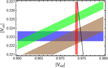
Figure 1: A combined plot of $|V_{ud}|$ from superallowed beta decays (red band), $|V_{us}|$ from $K_{\ell 3}$ (blue band), $|V_{us}/V_{ud}|$ from $R_{A}$ (green band) and $R_{V}$ (brown band), together with the first-row CKM unitarity requirement (black line). Notice that the blue and brown bands are highly correlated as they rely on the same set of inputs from $K_{\ell 3}$, so they should not be taken as independent constraints.

We close this section by reporting the current extracted values of $|V_{us}/V_{ud}|$ from $R_{A}$ and $R_{V}$ respectively, by supplementing Eq. (68) with relevant lattice QCD inputs FLA :

$$\begin{array}[]{ccc}|f_{K^{+}}/f_{\pi^{+}}|=1.1932(21)&\quad N_{f}=2+1+1&\quad\text{Refs.\cite[cite]{\@@bibref{Authors Phrase1YearPhrase2}{Bazavov:2017lyh,Dowdall:2013rya,Carrasco:2014poa,Miller:2020xhy}{\@@citephrase{(}}{\@@citephrase{)}}}}\\ |f_{+}^{K}(0)/f_{+}^{\pi}(0)|\approx|f_{+}^{K}(0)|=0.9698(17)\leavevmode\nobreak\ .&\quad N_{f}=2+1+1&\text{Refs.\cite[cite]{\@@bibref{Authors Phrase1YearPhrase2}{Carrasco:2016kpy,Bazavov:2018kjg}{\@@citephrase{(}}{\@@citephrase{)}}}}\end{array}$$ (70)

They give:

$$|V_{us}/V_{ud}|=\left\{\begin{array}[]{ccc}0.23131(41)_{\mathrm{lat}}(24)_{\mathrm{exp}}(19)_{\mathrm{RC}}&&\text{from $R_{A}$}\\ 0.22908(66)_{\mathrm{BR}(\pi_{e3})}(41)_{K}(40)_{\mathrm{lat}}(2)_{\tau_{\pi^{+}}}(1)_{\mathrm{RC}_{\pi}}&&\text{from $R_{V}$}\end{array}\right.\leavevmode\nobreak\ .$$ (71)

The difference between the two determinations is at the level of $2.2\sigma$. All the determinations of $|V_{us}|$, $|V_{ud}|$ and their ratio quoted in this paper are summarized in Fig.1, from which the mutual disagreements between different determinations and the deviations from the first-row CKM unitary requirement are clearly shown.

IV Conclusions

This work updates the values of $|V_{us}|$ and $|V_{us}/V_{ud}|$ determined from kaon and pion semileptonic decays using the most recent inputs from theory and experiment. The uncertainties in these quantities have been experiment- and lattice-dominated, which is even more the case in the recent years due to the more precise SM electroweak theory inputs. Their values along with $V_{ud}$ from superallowed beta decays correspond to 2–3$\sigma$ deviations from CKM unitary and related axial current induced weak decays. Those differences may provide hints of BSM physics or deficiencies in SM theory or experiment. Such anomalies provide a strong motivation for future improvements of the experimental precision of the $\pi_{e3}$ BR as well as the kaon lifetimes and $K_{\ell 3}$ BRs.

The experiment-dominated uncertainties do not imply that future improvements from the theory side are not important. It is quite the opposite; the aforementioned anomalies require us to carefully reexamine all the SM theory inputs in order to ensure that no unexpected large systematic errors exist. This was recently done for the long-distance EM corrections to the $K_{e3}$ decay rate and no large corrections were found. Other inputs, such as the lattice calculations of $f_{+}^{K}(0)$ and $f_{K^{+}}/f_{\pi^{+}}$, should be cross-checked with the same level of rigor. There are several other theory works that remain to be done for completeness and internal consistency: For instance, the reevaluation of the EM corrections should be generalized to the $K\mu$ channels, and the fitting of the $K\pi$ form factors should, in principle, also be updated to account for the modified EM corrections to the $K_{\ell 3}$ Dalitz plot.

Appendix A Mathematical Tools

In this Appendix, we review all the mathematical tools needed in this work.

A.1 Covariance matrix and correlation matrix

For a set of variables $X=(x_{1},x_{2},...,x_{n})^{T}$, we define the symmetric covariance matrix $\mathrm{Cov}(X)$ as:

$$\mathrm{Cov}(X)_{ij}=\left\langle x_{i}x_{j}\right\rangle-\left\langle x_{i}\right\rangle\left\langle x_{j}\right\rangle\leavevmode\nobreak\ .$$ (72)

In particular, the diagonal terms give the variance of $x_{i}$:

$$\sigma_{i}^{2}=\mathrm{Cov}(X)_{ii}\leavevmode\nobreak\ .$$ (73)

We also define the symmetric correlation matrix $\mathrm{Corr}(X)$ as:

$$\mathrm{Corr}(X)_{ij}=\frac{\left\langle x_{i}x_{j}\right\rangle-\left\langle x_{i}\right\rangle\left\langle x_{j}\right\rangle}{\sigma_{i}\sigma_{j}}\leavevmode\nobreak\ .$$ (74)

Its diagonal elements are always 1, while the off-diagonal elements range between $-1$ and 1. Its relation to the covariance matrix is given by:

$$\mathrm{Cov}(X)=\sigma_{X}\cdot\mathrm{Corr}(X)\cdot\sigma_{X}\leavevmode\nobreak\ ,$$ (75)

where $\sigma_{X}\equiv\mathrm{diag}(\sigma_{1},\sigma_{2},...,\sigma_{n})$.

A.2 Propagation of the covariance matrix

For a set of variables $F=(f_{1},f_{2},...,f_{m})^{T}$ that are functions of $X$ (i.e. $f_{i}=f_{i}(x_{1},...,x_{n})$), given the covariance matrix of $X$ we can immediately obtain the covariance matrix of $F$ as:

$$\mathrm{Cov}(F)=\left(\frac{\partial F}{\partial X}\right)\cdot\mathrm{Cov}(X)\cdot\left(\frac{\partial F}{\partial X}\right)^{T}$$ (76)

where $\partial F/\partial X$ is a $m\times n$ matrix, with matrix elements:

$$\left(\frac{\partial F}{\partial X}\right)_{ij}=\frac{\partial f_{i}}{\partial x_{j}}\leavevmode\nobreak\ .$$ (77)

If $F=(f_{1},f_{2},...,f_{m})^{T}$ depends on two independent sets of variables $X=(x_{1},x_{2},...,x_{n})^{T}$ and $Y=(y_{1},y_{2},...,y_{n^{\prime}})^{T}$ with their respective covariance matrices given, then the covariance matrix of $F$ is simply the sum of the two contributions:

$$\mathrm{Cov}(F)=\left(\frac{\partial F}{\partial X}\right)\cdot\mathrm{Cov}(X)\cdot\left(\frac{\partial F}{\partial X}\right)^{T}+\left(\frac{\partial F}{\partial Y}\right)\cdot\mathrm{Cov}(Y)\cdot\left(\frac{\partial F}{\partial Y}\right)^{T}\leavevmode\nobreak\ .$$ (78)

This is also generalizable if $F$ is a function of more than two independent sets of variables.

For definiteness, throughout this work, we always calculate partial derivatives numerically as:

$$\frac{\partial f}{\partial a}\approx\frac{f(a+\delta a)-f(a-\delta a)}{2\delta a}\leavevmode\nobreak\ .$$ (79)

A.3 Weighted average

If $X=(x_{1},x_{2},...,x_{n})^{T}$ has a covariance matrix $\mathrm{Cov}(X)$, then the weighted average between $x_{1},...,x_{n}$ is given by:

$$\bar{x}=\sigma_{\bar{x}}^{2}\left(J^{T}WX\right)$$ (80)

where the variance of $\bar{x}$ is given by:

$$\sigma_{\bar{x}}^{2}=\left(J^{T}WJ\right)^{-1}\leavevmode\nobreak\ .$$ (81)

Here we have defined $W=\left[\mathrm{Cov}(X)\right]^{-1}$ and $J=(1,...,1)^{T}$ (length = $n$).

References

- Zyla et al. (2020) P. Zyla et al. (Particle Data Group), PTEP 2020, 083C01 (2020).
- Abi et al. (2021) B. Abi et al. (Muon g-2), Phys. Rev. Lett. 126, 141801 (2021).
- Aoyama et al. (2020) T. Aoyama et al., Phys. Rept. 887, 1 (2020), eprint 2006.04822.
- Miller et al. (2007) J. P. Miller, E. de Rafael, and B. L. Roberts, Rept. Prog. Phys. 70, 795 (2007), eprint hep-ph/0703049.
- Miller et al. (2012) J. P. Miller, E. de Rafael, B. L. Roberts, and D. Stöckinger, Ann. Rev. Nucl. Part. Sci. 62, 237 (2012).
- Jegerlehner and Nyffeler (2009) F. Jegerlehner and A. Nyffeler, Phys. Rept. 477, 1 (2009), eprint 0902.3360.
- Aaij et al. (2019) R. Aaij et al. (LHCb), Phys. Rev. Lett. 122, 191801 (2019), eprint 1903.09252.
- Aaij et al. (2014) R. Aaij et al. (LHCb), Phys. Rev. Lett. 113, 151601 (2014), eprint 1406.6482.
- Aaij et al. (2015) R. Aaij et al. (LHCb), Phys. Rev. Lett. 115, 111803 (2015), [Erratum: Phys.Rev.Lett. 115, 159901 (2015)], eprint 1506.08614.
- Aaij et al. (2016) R. Aaij et al. (LHCb), JHEP 02, 104 (2016), eprint 1512.04442.
- Seng et al. (2018) C.-Y. Seng, M. Gorchtein, H. H. Patel, and M. J. Ramsey-Musolf, Phys. Rev. Lett. 121, 241804 (2018), eprint 1807.10197.
- Seng et al. (2019) C. Y. Seng, M. Gorchtein, and M. J. Ramsey-Musolf, Phys. Rev. D100, 013001 (2019), eprint 1812.03352.
- Czarnecki et al. (2019) A. Czarnecki, W. J. Marciano, and A. Sirlin, Phys. Rev. D 100, 073008 (2019), eprint 1907.06737.
- Seng et al. (2020a) C.-Y. Seng, X. Feng, M. Gorchtein, and L.-C. Jin, Phys. Rev. D 101, 111301 (2020a), eprint 2003.11264.
- Hayen (2021a) L. Hayen, Phys. Rev. D 103, 113001 (2021a), eprint 2010.07262.
- Hayen (2021b) L. Hayen (2021b), eprint 2102.03458.
- Shiells et al. (2021) K. Shiells, P. G. Blunden, and W. Melnitchouk, Phys. Rev. D 104, 033003 (2021), eprint 2012.01580.
- Seng (2021) C.-Y. Seng, Particles 4, 397 (2021), eprint 2108.03279.
- Hardy and Towner (2020) J. C. Hardy and I. S. Towner, Phys. Rev. C 102, 045501 (2020).
- Bryman and Shrock (2019a) D. Bryman and R. Shrock, Phys. Rev. D 100, 053006 (2019a), eprint 1904.06787.
- Bryman and Shrock (2019b) D. Bryman and R. Shrock, Phys. Rev. D 100, 073011 (2019b), eprint 1909.11198.
- Kirk (2021) M. Kirk, Phys. Rev. D 103, 035004 (2021), eprint 2008.03261.
- Grossman et al. (2020) Y. Grossman, E. Passemar, and S. Schacht, JHEP 07, 068 (2020), eprint 1911.07821.
- Belfatto et al. (2020) B. Belfatto, R. Beradze, and Z. Berezhiani, Eur. Phys. J. C 80, 149 (2020), eprint 1906.02714.
- Cheung et al. (2020) K. Cheung, W.-Y. Keung, C.-T. Lu, and P.-Y. Tseng, JHEP 05, 117 (2020), eprint 2001.02853.
- Jho et al. (2020) Y. Jho, S. M. Lee, S. C. Park, Y. Park, and P.-Y. Tseng, JHEP 04, 086 (2020), eprint 2001.06572.
- Yue and Cheng (2021) C. X. Yue and X. J. Cheng, Nucl. Phys. B 963, 115280 (2021), eprint 2008.10027.
- Endo and Mishima (2020) M. Endo and S. Mishima, JHEP 08, 004 (2020), eprint 2005.03933.
- Capdevila et al. (2021) B. Capdevila, A. Crivellin, C. A. Manzari, and M. Montull, Phys. Rev. D 103, 015032 (2021), eprint 2005.13542.
- Eberhardt et al. (2021) O. Eberhardt, A. P. n. Martínez, and A. Pich, JHEP 05, 005 (2021), eprint 2012.09200.
- Crivellin and Hoferichter (2020) A. Crivellin and M. Hoferichter, Phys. Rev. Lett. 125, 111801 (2020), eprint 2002.07184.
- Coutinho et al. (2020) A. M. Coutinho, A. Crivellin, and C. A. Manzari, Phys. Rev. Lett. 125, 071802 (2020), eprint 1912.08823.
- Gonzalez-Alonso et al. (2019) M. Gonzalez-Alonso, O. Naviliat-Cuncic, and N. Severijns, Prog. Part. Nucl. Phys. 104, 165 (2019), eprint 1803.08732.
- Falkowski et al. (2019) A. Falkowski, M. González-Alonso, and Z. Tabrizi, JHEP 05, 173 (2019), eprint 1901.04553.
- Cirigliano et al. (2019a) V. Cirigliano, A. Garcia, D. Gazit, O. Naviliat-Cuncic, G. Savard, and A. Young (2019a), eprint 1907.02164.
- Falkowski et al. (2021) A. Falkowski, M. González-Alonso, and O. Naviliat-Cuncic, JHEP 04, 126 (2021), eprint 2010.13797.
- Bečirević et al. (2021) D. Bečirević, F. Jaffredo, A. Peñuelas, and O. Sumensari, JHEP 05, 175 (2021), eprint 2012.09872.
- Crivellin et al. (2021a) A. Crivellin, M. Hoferichter, and C. A. Manzari, Phys. Rev. Lett. 127, 071801 (2021a), eprint 2102.02825.
- Tan (2019) W. Tan (2019), eprint 1906.10262.
- Crivellin et al. (2021b) A. Crivellin, M. Hoferichter, M. Kirk, C. A. Manzari, and L. Schnell, JHEP 10, 221 (2021b), eprint 2107.13569.
- Crivellin et al. (2020) A. Crivellin, F. Kirk, C. A. Manzari, and M. Montull, JHEP 12, 166 (2020), eprint 2008.01113.
- Crivellin et al. (2021c) A. Crivellin, F. Kirk, C. A. Manzari, and L. Panizzi, Phys. Rev. D 103, 073002 (2021c), eprint 2012.09845.
- Dekens et al. (2021) W. Dekens, L. Andreoli, J. de Vries, E. Mereghetti, and F. Oosterhof, JHEP 11, 127 (2021), eprint 2107.10852.
- Belfatto and Berezhiani (2021) B. Belfatto and Z. Berezhiani, JHEP 10, 079 (2021), eprint 2103.05549.
- Antonelli et al. (2010) M. Antonelli et al. (FlaviaNet Working Group on Kaon Decays), Eur. Phys. J. C 69, 399 (2010), eprint 1005.2323.
- Abouzaid et al. (2011) E. Abouzaid et al. (KTeV), Phys. Rev. D 83, 092001 (2011), eprint 1011.0127.
- Ambrosino et al. (2011) F. Ambrosino et al. (KLOE), Eur. Phys. J. C 71, 1604 (2011), eprint 1011.2668.
- Babusci et al. (2020) D. Babusci et al. (KLOE-2), Phys. Lett. B 804, 135378 (2020), eprint 1912.05990.
- Ma et al. (2021) P.-X. Ma, X. Feng, M. Gorchtein, L.-C. Jin, and C.-Y. Seng, Phys. Rev. D 103, 114503 (2021), eprint 2102.12048.
- Seng et al. (2021a) C.-Y. Seng, D. Galviz, M. Gorchtein, and U. G. Meißner, Phys. Lett. B 820, 136522 (2021a), eprint 2103.00975.
- Seng et al. (2021b) C.-Y. Seng, D. Galviz, M. Gorchtein, and U.-G. Meißner, JHEP 11, 172 (2021b), eprint 2103.04843.
- Cirigliano et al. (2019b) V. Cirigliano, E. Passemar, and M. Moulson (2019b), extraction of from experimetnal measurements, Proceedings of the International Conference on Kaon Physics 2019, https://indico.cern.ch/event/769729/contributions/3512047/attachments/1905114/3146148/Kaon2019_MoulsonPassemarCorr.pdf.
- Aoki et al. (2020) S. Aoki et al. (Flavour Lattice Averaging Group), Eur. Phys. J. C 80, 113 (2020), eprint 1902.08191.
- Moulson (2017) M. Moulson, PoS CKM2016, 033 (2017), eprint 1704.04104.
- Passemar and Moulson (2018) E. Passemar and M. Moulson (2018), status of determination from Kaon decays, 10th International Workshop on the CKM Unitarity Triangle, https://indico.cern.ch/event/684284/contributions/3075795/attachments/1717847/2775032/CKM2018_MoulsonPassemar.pdf.
- Czarnecki et al. (2020) A. Czarnecki, W. J. Marciano, and A. Sirlin, Phys. Rev. D 101, 091301 (2020), eprint 1911.04685.
- Feng et al. (2020) X. Feng, M. Gorchtein, L.-C. Jin, P.-X. Ma, and C.-Y. Seng, Phys. Rev. Lett. 124, 192002 (2020), eprint 2003.09798.
- Hertzog (2021) D. Hertzog (2021), a next-generation rare pion decay experiment to study LFUV and CKM unitarity, The 16th International Workshop on Tau Lepton Physics (TAU2021), https://indico.cern.ch/event/848732/contributions/4507273/attachments/2317723/3947483/Hertzog-TauLepton-2021.pdf.
- (59) A. Aguilar-Arevalo et al., Testing Lepton Flavor Universality and CKM Unitarity with Rare Pion Decay, https://www.snowmass21.org/docs/files/summaries/RF/SNOWMASS21-RF2_RF3-048.pdf.
- Marciano and Sirlin (1993) W. J. Marciano and A. Sirlin, Phys. Rev. Lett. 71, 3629 (1993).
- Erler (2004) J. Erler, Rev. Mex. Fis. 50, 200 (2004), eprint hep-ph/0211345.
- (62) Website: https://pdglive.lbl.gov/.
- Ambrosino et al. (2006a) F. Ambrosino et al. (KLOE), Phys. Lett. B 632, 43 (2006a), eprint hep-ex/0508027.
- Ambrosino et al. (2005) F. Ambrosino et al. (KLOE), Phys. Lett. B 626, 15 (2005), eprint hep-ex/0507088.
- Vosburgh et al. (1972) K. G. Vosburgh, T. J. Devlin, R. J. Esterling, B. Goz, D. A. Bryman, and W. E. Cleland, Phys. Rev. D 6, 1834 (1972).
- Alexopoulos et al. (2004) T. Alexopoulos et al. (KTeV), Phys. Rev. D 70, 092006 (2004), eprint hep-ex/0406002.
- Lai et al. (2002) A. Lai et al. (NA48), Phys. Lett. B 537, 28 (2002), eprint hep-ex/0205008.
- Bertanza et al. (1997) L. Bertanza et al., Z. Phys. C 73, 629 (1997).
- Schwingenheuer et al. (1995) B. Schwingenheuer et al., Phys. Rev. Lett. 74, 4376 (1995).
- Gibbons et al. (1993) L. K. Gibbons et al., Phys. Rev. Lett. 70, 1199 (1993).
- Batley et al. (2007) J. R. Batley et al., Phys. Lett. B 653, 145 (2007).
- Ambrosino et al. (2006b) F. Ambrosino et al. (KLOE), Phys. Lett. B 636, 173 (2006b), eprint hep-ex/0601026.
- Aloisio et al. (2002) A. Aloisio et al. (KLOE), Phys. Lett. B 535, 37 (2002), eprint hep-ph/0203232.
- Ambrosino et al. (2008a) F. Ambrosino et al. (KLOE), JHEP 01, 073 (2008a), eprint 0712.1112.
- Koptev et al. (1995) V. P. Koptev et al., JETP Lett. 61, 877 (1995).
- Ott and Pritchard (1971) R. J. Ott and T. W. Pritchard, Phys. Rev. D 3, 52 (1971).
- Lobkowicz et al. (1969) F. Lobkowicz, A. C. Melissinos, Y. Nagashima, S. Tewksbury, H. Von Briesen, and J. D. Fox, Phys. Rev. 185, 1676 (1969).
- Fitch et al. (1965) V. L. Fitch, C. A. Quarles, and H. C. Wilkins, Phys. Rev. 140, B1088 (1965).
- Ambrosino et al. (2008b) F. Ambrosino et al. (KLOE), JHEP 02, 098 (2008b), eprint 0712.3841.
- Chiang et al. (1972) I. H. Chiang, J. L. Rosen, S. Shapiro, R. Handler, S. Olsen, and L. Pondrom, Phys. Rev. D 6, 1254 (1972).
- Cirigliano et al. (2012) V. Cirigliano, G. Ecker, H. Neufeld, A. Pich, and J. Portoles, Rev. Mod. Phys. 84, 399 (2012), eprint 1107.6001.
- Hill (2006) R. J. Hill, Phys. Rev. D 74, 096006 (2006), eprint hep-ph/0607108.
- Lichard (1997) P. Lichard, Phys. Rev. D 55, 5385 (1997), eprint hep-ph/9702345.
- Bernard et al. (2006) V. Bernard, M. Oertel, E. Passemar, and J. Stern, Phys. Lett. B638, 480 (2006), eprint hep-ph/0603202.
- Bernard et al. (2009) V. Bernard, M. Oertel, E. Passemar, and J. Stern, Phys. Rev. D80, 034034 (2009), eprint 0903.1654.
- Abouzaid et al. (2010) E. Abouzaid et al. (KTeV), Phys. Rev. D 81, 052001 (2010), eprint 0912.1291.
- Moulson (2021) M. Moulson (2021), vus from kaon decays, 11th International Workshop on the CKM Unitarity Triangle (CKM 2021), https://indico.cern.ch/event/891123/contributions/4601856/attachments/2351074/4011941/CKM202021.pdf.
- Gasser and Leutwyler (1985) J. Gasser and H. Leutwyler, Nucl. Phys. B 250, 517 (1985).
- (89) Website: http://flag.unibe.ch/2019/Media?action=AttachFile&do=get&target=FLAG_2020_webupdate.pdf.
- Blum et al. (2016) T. Blum et al. (RBC, UKQCD), Phys. Rev. D 93, 074505 (2016), eprint 1411.7017.
- Durr et al. (2011a) S. Durr, Z. Fodor, C. Hoelbling, S. D. Katz, S. Krieg, T. Kurth, L. Lellouch, T. Lippert, K. K. Szabo, and G. Vulvert, Phys. Lett. B 701, 265 (2011a), eprint 1011.2403.
- Durr et al. (2011b) S. Durr, Z. Fodor, C. Hoelbling, S. D. Katz, S. Krieg, T. Kurth, L. Lellouch, T. Lippert, K. K. Szabo, and G. Vulvert, JHEP 08, 148 (2011b), eprint 1011.2711.
- Bazavov et al. (2009) A. Bazavov et al. (MILC), PoS CD09, 007 (2009), eprint 0910.2966.
- Fodor et al. (2016) Z. Fodor, C. Hoelbling, S. Krieg, L. Lellouch, T. Lippert, A. Portelli, A. Sastre, K. K. Szabo, and L. Varnhorst, Phys. Rev. Lett. 117, 082001 (2016), eprint 1604.07112.
- Bazavov et al. (2018) A. Bazavov et al., Phys. Rev. D 98, 074512 (2018), eprint 1712.09262.
- Carrasco et al. (2014) N. Carrasco et al. (European Twisted Mass), Nucl. Phys. B 887, 19 (2014), eprint 1403.4504.
- Bazavov et al. (2014) A. Bazavov et al. (Fermilab Lattice, MILC), Phys. Rev. D 90, 074509 (2014), eprint 1407.3772.
- Giusti et al. (2017) D. Giusti, V. Lubicz, C. Tarantino, G. Martinelli, F. Sanfilippo, S. Simula, and N. Tantalo, Phys. Rev. D 95, 114504 (2017), eprint 1704.06561.
- Aoki et al. (2017) S. Aoki et al., Eur. Phys. J. C 77, 112 (2017), eprint 1607.00299.
- Colangelo et al. (2018) G. Colangelo, S. Lanz, H. Leutwyler, and E. Passemar, Eur. Phys. J. C 78, 947 (2018), eprint 1807.11937.
- Cirigliano et al. (2008) V. Cirigliano, M. Giannotti, and H. Neufeld, JHEP 11, 006 (2008), eprint 0807.4507.
- Sirlin (1978) A. Sirlin, Rev. Mod. Phys. 50, 573 (1978), [Erratum: Rev. Mod. Phys.50,905(1978)].
- Seng et al. (2020b) C.-Y. Seng, D. Galviz, and U.-G. Meißner, JHEP 02, 069 (2020b), eprint 1910.13208.
- Seng et al. (2020c) C.-Y. Seng, X. Feng, M. Gorchtein, L.-C. Jin, and U.-G. Meißner, JHEP 10, 179 (2020c), eprint 2009.00459.
- Giusti et al. (2018) D. Giusti, V. Lubicz, G. Martinelli, C. T. Sachrajda, F. Sanfilippo, S. Simula, N. Tantalo, and C. Tarantino, Phys. Rev. Lett. 120, 072001 (2018), eprint 1711.06537.
- (106) P. Boyle et al., High-precision determination of and from lattice QCD. [Link].
- Carrasco et al. (2016) N. Carrasco, P. Lami, V. Lubicz, L. Riggio, S. Simula, and C. Tarantino, Phys. Rev. D 93, 114512 (2016), eprint 1602.04113.
- Bazavov et al. (2019) A. Bazavov et al. (Fermilab Lattice, MILC), Phys. Rev. D99, 114509 (2019), eprint 1809.02827.
- Bazavov et al. (2013) A. Bazavov et al., Phys. Rev. D 87, 073012 (2013), eprint 1212.4993.
- Boyle et al. (2015) P. A. Boyle et al. (RBC/UKQCD), JHEP 06, 164 (2015), eprint 1504.01692.
- Lubicz et al. (2009) V. Lubicz, F. Mescia, S. Simula, and C. Tarantino (ETM), Phys. Rev. D 80, 111502 (2009), eprint 0906.4728.
- Gorchtein (2019) M. Gorchtein, Phys. Rev. Lett. 123, 042503 (2019), eprint 1812.04229.
- Marciano (2004) W. J. Marciano, Phys. Rev. Lett. 93, 231803 (2004), eprint hep-ph/0402299.
- Cirigliano and Neufeld (2011) V. Cirigliano and H. Neufeld, Phys. Lett. B 700, 7 (2011), eprint 1102.0563.
- Behrends and Sirlin (1960) R. E. Behrends and A. Sirlin, Phys. Rev. Lett. 4, 186 (1960).
- Ademollo and Gatto (1964) M. Ademollo and R. Gatto, Phys. Rev. Lett. 13, 264 (1964).
- Pocanic et al. (2004) D. Pocanic et al., Phys. Rev. Lett. 93, 181803 (2004), eprint hep-ex/0312030.
- (118) David Hertzog, private communication.
- Dowdall et al. (2013) R. J. Dowdall, C. T. H. Davies, G. P. Lepage, and C. McNeile, Phys. Rev. D 88, 074504 (2013), eprint 1303.1670.
- Carrasco et al. (2015) N. Carrasco et al., Phys. Rev. D 91, 054507 (2015), eprint 1411.7908.
- Miller et al. (2020) N. Miller et al., Phys. Rev. D 102, 034507 (2020), eprint 2005.04795.